A unified approach to model estimation and controller reduction (duality and coherence)

A Unified Approach to Model Estimation and

Controller Reduction (Duality and Coherence)

I.D. LandauLaboratoire d’Automatique de Grenoble (CNRS-INPG-UJF)

ENSIEG, BP. 46, 38402 St. Martin d’Heres, France.e-mail:[email protected]

A. Karimi

Laboratoire d’Automatique, Ecole Polytechnique Federale deLausanne (EPFL), CH1015 Lausanne, Switzerland.

e-mail: [email protected]

Abstract

Closed loop output error identification algorithms [7, 9]and recentlydeveloped algorithms for direct closed loop estimation of reduced ordercontrollers [8] despite their diversity have in fact a unifying basic groundwhich will be enhanced.

In this paper it is shown that the plant model identification in closedloop using closed loop output error identification algorithms and the directestimation in closed loop of a reduced order controller feature a dualitycharacter. Basic schemes, algorithms and properties of the algorithms canbe directly obtained by interchanging the plant model and the controller.Additional schemes and algorithms allowing a full coverage of the variouspossible identification and reduction criteria are given.

The paper also will explore the coherence aspects in using closed loopplant model identification and direct estimation in closed loop of reducedorder controllers. The following problem will be addressed: what closedloop plant model identification should be used when a criterion for con-troller reduction is given?

Keywords: System identification, closed loop identification, controllerreduction.

1

1 Introduction

Closed loop output error (CLOE) identification algorithms [7, 9] allow an ap-proximate design model to be identified which features a high accuracy in thecritical regions for control design. Effectively the frequency distribution of theasymptotic error (bias) between the estimated and the true model is heavilyweighted by the magnitude of the sensitivity function of the true system whichexplains why this desired property is obtained.

In fact the algorithms search for a plant model which minimizes a 2-normerror between the true closed loop transfer function and the simulated closedloop transfer function containing the final estimated model.

Asymptotic frequency bias error distribution can be obtained indicatingclearly that the bias is small where some sensitivity functions are high andin addition this bias error is not asymptotically affected by the measurementnoise [5, 3].

Several configurations for the closed loop output error identification can beestablished. While the parameter adaptation algorithm (PAA) is basically thesame, the identification criterion and the asymptotic properties of the estimatedmodel will be different.

It is well known that controller order reduction should aim to preserve therequired closed loop properties as far as possible [1]. It has been shown in thepaper [8] that this can be performed by estimation in closed loop of reducedorder controllers either using simulated data or real data (which is a uniquefeature of this approach with respect to other approaches to direct controllerreduction). To proceed one needs to know the nominal controller and to havean estimated plant model (either the model used for design or a model identifiedon site in open or closed loop). The algorithms developed for the estimation ofreduced order controllers minimize a 2-norm of the difference between the nom-inal sensitivity function and the one obtained with the reduced order controller(i.e. they try to preserve the nominal closed loop properties). The algorithmshave the property that the error between the reduced order controller and thenominal controller is small at the frequencies where some sensitivity functionsare high.

Several configurations can be considered each corresponding to specific con-troller reduction criterion. However the PAA is in fact basically the same.

The first objective of the paper is to give a unified ground for the variousschemes proposed for closed loop output error identification and direct closedloop estimation of reduced order controllers by observing that in each schemethe algorithm searches for the approximation of a specific closed loop sensitiv-ity function. This investigation led to the observation that there were missedschemes and algorithms which are presented here for the first time.

The second objective of the paper is to show that these two problems (modelestimation and controller reduction) are dual and that the effective algorithms,the stability analysis and the asymptotic properties can be obtained by a directsubstitution i.e.:

2

p(t)v(t)

K Gr(t) u(t) y(t)

-

+ +

Figure 1: The closed-loop system

estimated plant model −→ estimated controller;

nominal controller −→ plant model.

The only differences will occur at the effective implementation of the algorithmssince the controller has a direct transfer term while the plant model has at leastone step delay.

The third objective of the paper is to explore the coherent use of closed loopplant model identification in direct controller order reduction. The followingproblem will be addressed: what closed loop plant model identification shouldbe used when a criterion for direct controller reduction is given?

The paper is organized as follows. Section 2 will specify the notations. Sec-tion 3 will survey the various configurations for closed loop plant model identi-fication and their properties. Section 4 will explore the various configurationsfor direct estimation in closed loop of reduced order controllers and their prop-erties. Section 5 will give the basic algorithms for closed loop identification andtheir frequency bias distributions. The algorithms for controller order reductionwill be derived from the closed loop identification algorithms via duality in Sec-tion 6. Section 7 will discuss the coherency between closed loop identificationand direct controller reduction. A simulation example in Section 8 illustratesthe discussed properties of the algorithms. Finally some concluding remarkswill be given.

2 Notations

Consider the system shown in Fig. 1, where the plant model is given by:

G(z−1) =z−dB(z−1)A(z−1)

(1)

and

A(z−1) = 1 + a1z−1 + · · ·+ anAz

−nA

= 1 + z−1A∗(z−1) (2)B(z−1) = b1z

−1 + · · ·+ bnBz−nB

= z−1B∗(z−1) (3)

3

In Fig. 1, r(t) is generically the external excitation (which can be applied alsoat other points). v(t) and p(t) correspond respectively to input and outputdisturances. It is supposed that the plant model is an exact representation ofthe true system. The plant model is also characterized by a parameter vector:

θ∗T = [a1 · · · anA , b1 · · · bnB ] (4)

The nominal controller is given by:

K(z−1) =R(z−1)S(z−1)

(5)

where

R(z−1) = r0 + r1z−1 + · · ·+ rnRz

−nR (6)S(z−1) = 1 + s1z

−1 + · · ·+ snSz−nS

= 1 + z−1S∗(z−1) (7)

The nominal controller is a high-order controller computed on the basis of anavailable nominal plant model (and not in the basis of the true plant model (1))that meets the control specifications for the nominal closed-loop system. Thecontroller is also characterized by a parameter vector:

θ∗cT = [r0, r1 · · · rnR , s1 · · · snS ] (8)

The following sensitivity functions are defined:

• Syp(z−1) =1

1 + KG=

A(z−1)S(z−1)P (z−1)

;

• Sup(z−1) =−K

1 + KG=−A(z−1)R(z−1)

P (z−1);

• Syv(z−1) =G

1 + KG=

z−dB(z−1)S(z−1)P (z−1)

;

• Syr(z−1) =KG

1 + KG=

z−dB(z−1)R(z−1)P (z−1)

.

whereP (z−1) = A(z−1)S(z−1) + z−dB(z−1)R(z−1) (9)

is the closed loop characteristic polynomial. Note that the first subscript letterdefines the output point and the second letter the input point for the evaluationof the sensitivity functions.

The system of Fig.1 will be denoted the “true closed loop system”. Through-out the paper we will consider feedback systems which will use either an esti-mation of G (denoted G) or a reduced order estimation of K (denoted K). Thecorresponding sensitivity functions will be denoted as follows:

4

• Sxy - Sensitivity function of the true closed loop system (K, G).

• Sxy - Sensitivity function of the nominal simulated closed loop system(nominal controller K + estimated plant model G).

• ˆSxy - Sensitivity function of the simulated closed loop system using areduced order controller (reduced controller K + estimated plant modelG).

Similar notations are used for P (z−1): P (z−1) when using K and G, ˆP (z−1)

when using K and G.

3 Closed loop identification schemes

Figures 2a, 2b and 2c summarize the various configurations belonging to theclosed loop identification algorithms.

We will indicate next the identification criterion corresponding to each con-figuration.a) Closed loop output error with external excitation added to the controller input(Fig. 2a): The identification criterion in this case is:

θ∗ = arg minθ

∥∥∥Syr − Syr

∥∥∥2

= arg minθ

∥∥∥Syp − Syp

∥∥∥2

(10)

= arg minθ

∥∥∥Syp(G− G)Sup∥∥∥

2(11)

b) Closed loop output error with external excitation added to the plant input(Fig. 2b): The identification criterion in this case is:

θ∗ = arg minθ

∥∥∥Syv − Syv

∥∥∥2

= arg minθ

∥∥∥Syp(G− G)Syp∥∥∥

2(12)

c) Closed loop input error with external excitation added to the controller input(Fig. 2c): The identification criterion in this case is:

θ∗ = arg minθ

∥∥∥Sup − Sup

∥∥∥2

= arg minθ

∥∥∥Sup(G− G)Sup∥∥∥

2(13)

As one can see these three configurations cover all the possible closed loopidentification criteria (one can match all the four sensitivity functions). Notethat one can consider a fourth configuration corresponding to a closed loopinput error with external excitation added to the plant input. However thisconfiguration corresponds to the one of Fig. 2a where in the upper part (thetrue system) the place of K and G is interchanged. This, however, will notchange the identification criterion for SISO systems.

In short for the configuration of Fig. 2a, 2b and 2c, if r(t) is a discretetime white noise (for example a PRBS which is a good approximation) thealgorithm will search for the best G which will minimize the 2-norm between

5

K G

G

r

u

uy

y+

+

+−

−

−

P.A.A.

CLε

K

+

+p

Figure 2a: Closed loop output error (CLOE) (external excitation added to thecontroller input)

K

P . A . A .

G

r

u

u y

y

CLε

+

+

+

−

−

−

K

G

p

+

+

Figure 2b: Closed loop output error (CLOE) (external excitation added to theplant input)

K

G

P . A . A .

G

rc u

c u

y

y CLε

+

+

+

−

−

−

K

p++

Figure 2c: Closed loop input error (CLIE) (external excitation added to thecontroller input)

6

the various sensitivity functions. In addition the differences between G and Gwill be minimized in the frequency regions where the sensitivity functions havelarge values.

The first practical consequence is that the choice of one scheme or anotheris related to the main performance objective of the controller design (since themodel identified in closed loop in the context of this paper will be used for con-troller reduction of a nominal controller designed to match a desired sensitivityfunction). For tracking and output disturbance rejection it is preferable to usethe scheme of Fig. 2a. For output rejection of a disturbance entered at the inputof the plant it is preferred to use the scheme of Fig. 2b. For minimization of theeffect of the output disturbance on the controller input it is more appropriateto use the scheme of Fig. 2c.

The second practical consequence of these properties is that the choice of oneor other configuration should be done in relation with the type of uncertaintywhich is logical to be considered for controller design in a specific application.The reason is that the robust stability conditions are expressed in terms ofspecific sensitivity function for a given type of uncertainties and one would liketo best approximate this sensitivity function.

4 Direct estimation of reduced order controllers

We will consider that a model of the plant is available (denoted by G). Thismodel can be the plant model used for controller design or an identified model(in open loop or in closed loop) which passed the validation tests. We willassume of course that the nominal controller of orders nR and nS is known(denoted by K).

Figures 3a, 3b and 3c summarize the various configuration for direct esti-mation in closed loop of reduced order controllers. We will indicate next thecontroller reduction criterion for each configuration.a) Closed loop input matching with external excitation added to the plant input:The controller reduction criterion in this case is:

θ∗c = arg minθc

∥∥∥Syr − ˆSyr

∥∥∥2

= arg minθc

∥∥∥Syp − ˆSyp

∥∥∥2

(14)

b) Closed loop output matching with external excitation added to the plant input:The controller reduction criterion in this case is:

θ∗c = arg minθc

∥∥∥Syv − ˆSyv

∥∥∥2

(15)

c) Closed loop input matching with external excitation added to the controllerinput: The controller reduction criterion in this case is:

θ∗c = arg minθc

∥∥∥Sup − ˆSup

∥∥∥2

(16)

These three configurations cover all possible controller reduction criteriabased on preservation of the closed loop properties. Note that one can consider

7

x u

x û

nominal simulated closed - loop

reduced ordercontroller

Figure 3a: Closed loop input matching (CLIM) (external excitation added tothe plant input)

Figure 3b: Closed loop output matching (CLOM) (external excitation addedto the plant input)

x

x

Figure 3c: Closed loop input matching (CLIM) (external excitation added tothe controller input)

8

x y

nominal simulated closed - loop

reduced ordercontroller

GKyu

^

Figure 4: Closed loop output matching with external excitation added to thecontroller input

a fourth configuration corresponding to a closed loop output matching schemewith external excitation added to the controller input [6] (see Fig. 4). Howeverthis configuration corresponds to the one of Fig 3a where in the upper part (thenominal simulated system) the place of K and G is reverted.

When r(t) is a discrete white noise (for example a PBRS) the algorithms willsearch for the best controller K which will minimize the 2-norm of the controllerreduction criterion. Like in closed loop identification the differences between Kand K will be small at the frequencies where the sensitivity functions have largevalues.

The above schemes can be used also with real data [8]. In this case it canbe shown that the noise will not affect the minimization procedure.

5 Closed loop identification algorithms

The output of the plant is given by:

y(t + 1) = −A∗y(t) + B∗u(t− d) + Ap(t + 1) = θTψ(t) + Ap(t + 1) (17)

where

ψT (t) = [−y(t) . . .− y(t− nA + 1), u(t− d) . . . u(t− d− nB + 1)] (18)θT = [a1, . . . , anA , b1, . . . , bnB ] (19)

u(t) = − R

Sy(t) + ru(t) (20)

and ru(t) = r(t) in the scheme of Fig. 2b and ru(t) =R

Sr(t) in the scheme of

Fig. 2a and 2c.The output of the closed loop adjustable predictor is given by:

9

a priori:

y◦(t + 1) = −A∗(t, q−1)y(t) + B∗(t, q−1)u(t− d) = θT (t)φ(t) (21)

u(t) = −R(q−1)S(q−1)

y(t) + ru(t) (22)

a posteriori:y(t + 1) = θT (t + 1)φ(t) (23)

where

θT (t) = [a1, . . . , anA , b1, . . . , bnB ] (24)

φT (t) = [−y(t) . . .− y(t− nA + 1), u(t− d) . . . u(t− d− nB + 1)] (25)

5.1 Closed loop output error algorithms (CLOE)

The closed loop output error is defined as:a priori:

ε◦CL(t + 1) = y(t + 1)− y◦(t + 1)

a posteriori:εCL(t + 1) = y(t + 1)− y(t + 1)

and the parameter adaptation algorithm (PAA) is given by:

θ(t + 1) = θ(t) + F (t)Φ(t)εCL(t + 1) (26)F−1(t + 1) = λ1(t)F−1(t) + λ2(t)Φ(t)ΦT (t) (27)

0 < λ1(t) ≤ 1; 0 ≤ λ2(t) < 2; F (0) > 0

εCL(t + 1) =ε◦CL(t + 1)

1 + ΦT (t)F (t)Φ(t)(28)

Specific algorithms are obtained by an appropriate choice of the observationvector Φ(t) as follows:

CLOE Φ(t) = φ(t)

F-CLOE (Filtered CLOE) Φ(t) =S(q−1)P (q−1)

φ(t)

AF-CLOE (Adaptive Filtered CLOE) Φ(t) =S(q−1)P (t, q−1)

φ(t)

where:

P (q−1) = A(q−1)S(q−1) + q−dB(q−1)R(q−1)P (t, q−1) = A(t, q−1)S(q−1) + q−dB(t, q−1)R(q−1)

A(q−1) and B(q−1) correspond to an a priori estimation of G, while A(t, q−1)and B(t, q−1) correspond to the current estimates of G.

10

When nA = nA, nB = nB , then the closed loop output error goes to zero(in a deterministic environment: p(t) ≡ 0) and unbiased estimates are obtainedin a stochastic environment (when p(t) is independent with respect to ru(t) andof finite power) if:

H ′(z−1) = H(z−1)− λ

2; max

tλ2(t) ≤ λ < 2 (29)

is a strictly positive real transfer function, where:

H(z−1) =

S/P for CLOEP /P for F-CLOE1 for AF-CLOE

(30)

(in the last case this is a local result) [7, 9].When nA < nA, nB < nB , it can be shown that all the signals are bounded

provided that [7]:

– ru(t) is norm bounded;

– It exists a reduced order model such that:

y(t + 1)= −A∗(q−1) y(t) + B(q−1)u(t− d) + η(t + 1) (31)

where η(t + 1) is norm bounded for a norm bounded r(t);

– The passivity condition (29) is satisfied.

5.2 Closed loop input error algorithms (CLIE)

As it has already mentioned the closed loop input error scheme when the excita-tion signal is added to the plant input is equivalent to the CLOE algorithm withexternal excitation added to the controller input (they have the same identifi-cation criterion). Therefore we consider only the CLIE algorithm with externalexcitation added to the controller input.

The closed loop input error is in fact the closed loop output error filtered bythe controller transfer function (see Eqs. 20 and 22). Thus the same algorithmscan be used with the difference that the prediction error εCL is replaced with aposteriori adaptation error defined as follows:

ν(t + 1) = u(t + 1)− u(t + 1) = −R(q−1)S(q−1)

(y(t + 1)− y(t + 1))

= −R(q−1)S(q−1)

εCL(t + 1) (32)

or

ν(t + 1) = −S∗(q−1)ν(t)−R(q−1)εCL(t + 1)

= −S∗(q−1)ν(t)− r0εCL(t + 1)−nR∑i=1

riεCL(t− i + 1) (33)

11

Then the parameter adaptation algorithm will be given by:

θ(t + 1) = θ(t) + F (t)Φ(t)ν(t + 1) (34)F−1(t + 1) = λ1(t)F−1(t) + λ2(t)Φ(t)Φ(t)T (35)0 < λ1(t) ≤ 1; 0 ≤ λ2(t) < 2

Since ν(t+ 1) is not available before computing θ(t+ 1), it should be computedusing the a priori adaptation error defined by:

ν◦(t + 1) = −S∗(q−1)ν(t)− r0ε◦CL(t + 1)−

nR∑i=1

riεCL(t− i + 1) (36)

Subtracting Eq. 36 from Eq. 33, one obtains:

ν(t + 1)− ν◦(t + 1) = r0εCL(t + 1)− r0ε◦CL(t + 1)

= −r0[y◦(t + 1)− y(t + 1)]

= −r0[θ(t + 1)− θ(t)]TΦ(t)= −r0ΦT (t)F (t)Φ(t)ν(t + 1) (37)

Then the relation between the a posteriori and the a priori adaptation error isgiven by:

ν(t + 1) =ν◦(t + 1)

1 + r0ΦT (t)F (t)Φ(t)(38)

From this equation, one observes that the a posteriori adaptation error ν(t+ 1)may be unbounded for the negative value of r0 when the denominator approachesto zero. In order to fix this problem the a posteriori adaptation error can bemodified as follows:

ν(t + 1) = sign(r0)[u(t + 1)− u(t + 1)] = sign(r0)R(q−1

S(q−1)εCL(t + 1) (39)

where

sign(r0) ={

1 if r0 ≥ 0−1 otherwise

The new definition leads to the following relation between the a posteriori andthe a priori adaptation error:

ν(t + 1) =ν◦(t + 1)

1 + |r0|ΦT (t)F (t)Φ(t)(40)

Like the CLOE algorithms, specific algorithms can be obtained by an ap-propriate choice of the observation vector Φ(t) as follows:

CLIE Φ(t) = φ(t)

F-CLIE (Filtered CLIE) Φ(t) =R(q−1)P (q−1)

φ(t)

AF-CLIE (Adaptive Filtered CLIE) Φ(t) =R(q−1)P (t, q−1)

φ(t)

12

When nA = nA, nB = nB , then the closed loop input error goes to zero (in adeterministic environment: p(t) ≡ 0) and unbiased estimates are obtained in astochastic environment (when p(t) is independent with respect to ru(t) and offinite power) if H ′(z−1) is a strictly positive real transfer function, where:

H(z−1) =

R/P for CLIEP /P for F-CLIE1 for AF-CLIE

(41)

Remark: The closed loop input error can also be indirectly minimized by theCLOE algorithms using the excitation signal filtered by the controller transferfunction. In this case the stability and convergence condition for the algorithmis the same as the CLOE algorithms. The problems may occur when S(q−1) isunstable: On one hand the positive real condition on S/P is no longer satisfied(this problem can be solved using F-CLOE or AF-CLOE) and on the otherhand, the reference signal filtered by R/S becomes unbounded and cannot beapplied to the real system.

5.3 Asymptotic frequency bias distribution

The asymptotic frequency distribution of the bias when the estimated plantmodel does not belong to the model set for various configurations is given by[7, 5]:a) Closed loop output error with external excitation added to the controller input

θ∗ = arg minθ

∫ π

−π|Syp|2

[|G− G|2|Sup|2φr(ω) + φp(ω)

]dω

= arg minθ

∫ π

−π

[|Syr − Syr|2φr(ω) + |Syp|2φp(ω)

]dω (42)

b) Closed loop output error with external excitation added to the plant input

θ∗ = arg minθ

∫ π

−π|Syp|2

[|G− G|2|Syp|2φr(ω) + φp(ω)

]dω

= arg minθ

∫ π

−π

[|Syv − Syv|2φr(ω) + |Syp|2φp(ω)

]dω (43)

c) Closed loop input error with external excitation added to the controller input1

θ∗ = arg minθ

∫ π

−π|Sup|2

[|G− G|2|Sup|2φr(ω) + φp(ω)

]dω

= arg minθ

∫ π

−π

[|Sup − Sup|2φr(ω) + |Sup|2φp(ω)

]dω (44)

1These expressions are strictly valid when using AF-CLOE (case a and b) and AF-CLIE(case c). However CLOE and F-CLOE can be viewed as approximations of AF-CLOE andCLIE and F-CLIE can be viewed as approximations of AF-CLIE

13

These expressions show that if the external excitation r(t) is a white noise (or forexample a PRBS), the algorithms will search for the best G which will minimizethe 2-norm of error between the sensitivity functions of true closed loop systemand of the estimated closed loop system. Furthermore the noise will not affectthe asymptotic parameter estimation because output error criteria are used here.

6 Algorithms for estimation of reduced ordercontrollers

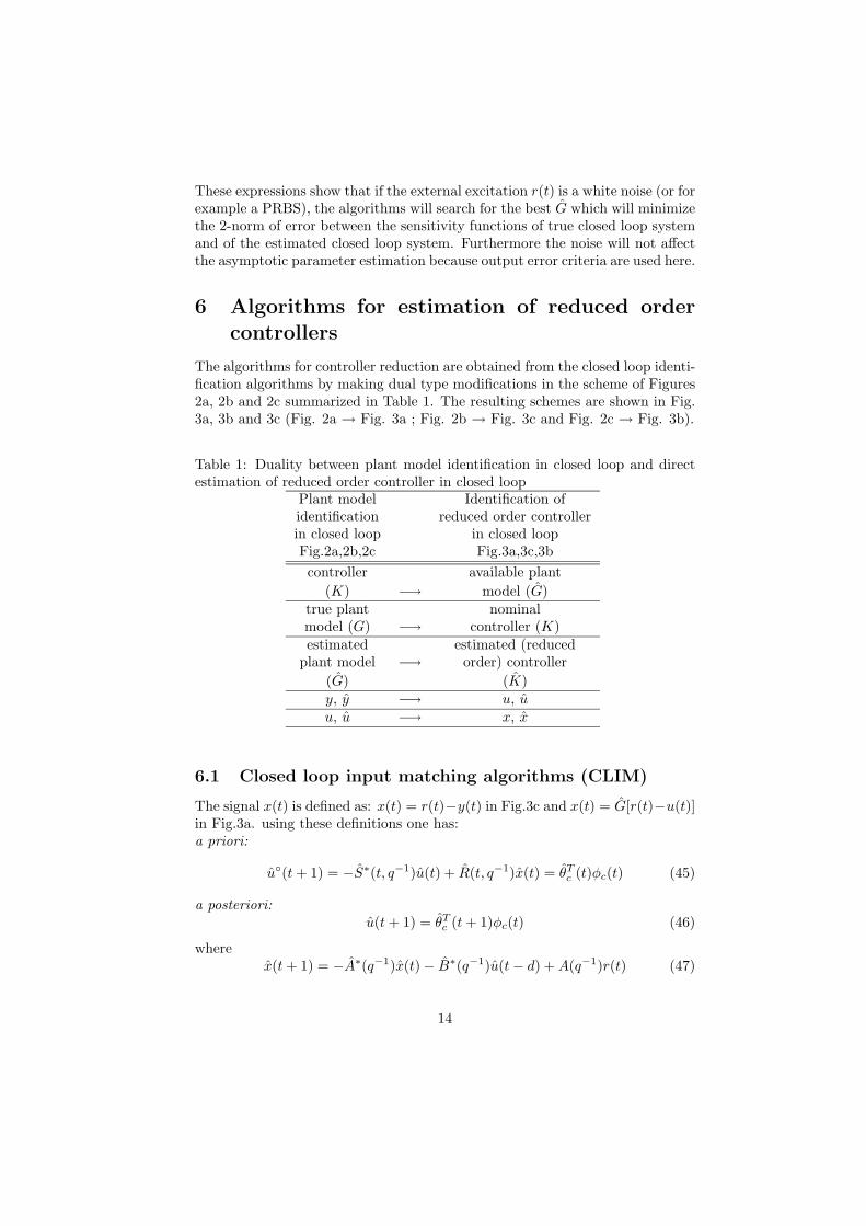
The algorithms for controller reduction are obtained from the closed loop identi-fication algorithms by making dual type modifications in the scheme of Figures2a, 2b and 2c summarized in Table 1. The resulting schemes are shown in Fig.3a, 3b and 3c (Fig. 2a → Fig. 3a ; Fig. 2b → Fig. 3c and Fig. 2c → Fig. 3b).

Table 1: Duality between plant model identification in closed loop and directestimation of reduced order controller in closed loop

Plant model Identification ofidentification reduced order controllerin closed loop in closed loopFig.2a,2b,2c Fig.3a,3c,3bcontroller available plant

(K) −→ model (G)true plant nominalmodel (G) −→ controller (K)estimated estimated (reduced

plant model −→ order) controller(G) (K)y, y −→ u, uu, u −→ x, x

6.1 Closed loop input matching algorithms (CLIM)

The signal x(t) is defined as: x(t) = r(t)−y(t) in Fig.3c and x(t) = G[r(t)−u(t)]in Fig.3a. using these definitions one has:a priori:

u◦(t + 1) = −S∗(t, q−1)u(t) + R(t, q−1)x(t) = θTc (t)φc(t) (45)

a posteriori:u(t + 1) = θTc (t + 1)φc(t) (46)

wherex(t + 1) = −A∗(q−1)x(t)− B∗(q−1)u(t− d) + A(q−1)r(t) (47)

14

for the scheme of Fig. 3c, and

x(t + 1) = −A∗(q−1)x(t)− B∗(q−1)u(t− d) + B∗r(t− d) (48)

for the scheme of Fig. 3a, and

θTc (t) = [s1(t), . . . , snS (t), r0(t), . . . , rnR(t)] (49)

φTc (t) = [−u(t), . . . ,−u(t− nS + 1), x(t + 1), . . . , x(t− nR + 1)] (50)

The closed loop input error will be given by:a priori:

ε◦CL(t + 1) = u(t + 1)− u◦(t + 1)

a posteriori:εCL(t + 1) = u(t + 1)− u(t + 1)

and the same PAA algorithm described in the Eqs. (26) through (28) can beused and the corresponding specific algorithms will be:

CLIM Φ(t) = φc(t)

F-CLIM Φ(t) =A(q−1)P (q−1)

φc(t)

where:P (q−1) = A(q−1)S(q−1) + q−d−1B(q−1)R(q−1)

is a known quantity and therefore there is no need to estimate this polynomial inline. The corresponding transfer functions involved in the passivity conditionsfor stability become:

H(z−1) =

A(q−1)P (q−1)

for CLIM

1 for F-CLIM

(since the exact polynomial of the nominal simulated closed loop is known).

6.2 Closed loop output matching algorithms (CLOM)

As it has already been noted the closed loop output matching algorithm whenthe excitation signal is added to the controller input (See Fig. 4) is equivalentto the CLIM with external excitation added to the plant input (see Fig. 3a).Therefore the same algorithm can be used for both cases which have the samecriterion.

For the CLOM algorithm when the excitation signal is added to the plantinput, two choices may be considered: The first one is to filter the excitationsignal through G and use the CLIM algorithm corresponding to the scheme inFig 3a. In this case, evidently, the stability and convergence condition of thealgorithm is the same as CLIM algorithm. The second choice is to derive directly

15

an algorithm for minimizing the closed loop output error. But this algorithmencounters a technical problem so that the convergence condition becomes B/Pwhich is never a positive real transfer function (because of at least one steptime delay in B). Although this problem can be fixed using a d + 1 step aheadprediction error, the first choice still seems to be more appropriate because inmany practical systems A is stable and the necessary condition for the positiverealness of A/P is satisfied.

6.3 Asymptotic frequency bias distribution

The crucial step is to examine the properties of the estimated reduced ordercontroller. To do this we will directly use the expressions (42) and (44) in whichwe will take φp(ω) = 0 (no noise) and we will make the substitution indicatedin Table 1. One gets for the asymptotic frequency distribution of the bias thefollowing expressions:a) Closed loop input matching with external excitation added to the plant input

θ∗c = arg minθc

∫ π

−π|Syp|2|K − K|| ˆSyv|φr(ω)dω

= arg minθc

∫ π

−π|Syr − ˆ

Syr|2φr(ω)dω (51)

b) Closed loop output matching with external excitation added to the plant input

θ∗c = arg minθc

∫ π

−π|Syp|2|K − K|| ˆSyv|φr(ω)dω

= arg minθc

∫ π

−π|Syv − ˆ

Syv|2φr(ω)dω (52)

c) Closed loop input matching with external excitation added to the controllerinput

θ∗c = arg minθc

∫ π

−π|Syp|2|K − K|| ˆSyp|φr(ω)dω

= arg minθc

∫ π

−π|Sup − ˆ

Sup|2φr(ω)dω (53)

When r(t) is a discrete time white noise these expressions correspond exactlyto the 2-norm expression which we would like to minimize in each case. It shouldbe noted that the resulting controller is the best reduced order controller withrespect to the nominal plant model G not to the true plant model G. However,it is the case for all of the controller reduction methods. A detailed analysiswhen one uses real data can be found in [8]. In this case it was shown that thenoise term does not affect the minimization procedure.

16

7 Coherency between model identification andcontroller reduction in closed loop

The interesting problem to address is: What closed loop plant model identifi-cation should be used when a criterion for direct controller reduction is given?To answer this question we will make reference to the iterative identification inclosed loop and controller re-design methodology [4, 10, 2]. The basic rule forimproving performance is to use the same criterion for identification in closedloop and controller re-design. In our case controller re-design corresponds tothe reduction of the nominal controller. Therefore examining the identificationcriterion for the various closed loop identification schemes and the controllerreduction objectives, a coherency is observed between them as indicated in Ta-ble 2.

Table 2: Coherent controller reduction and identification in closed loop

Controllerreduction criterion

Controller reductionscheme

Closed loopidentification scheme

min ‖Syp − ˆSyp‖

CLOM with externalexcitation added tothe controller input

CLOE with externalexcitation added tothe controller input

or or or

min ‖Syr − ˆSyr‖

CLIM with externalexcitation added tothe plant input

CLIE with externalexcitation added tothe plant input

min ‖Syv − ˆSyv‖

CLOM with externalexcitation added tothe plant input

CLOE with externalexcitation added tothe plant input

min ‖Sup − ˆSup‖

CLIM with externalexcitation added tothe controller input

CLIE with externalexcitation added tothe controller input

8 Simulation Example

The objective is to show the improvement of performance in controller reduc-tion when a coherent choice of closed loop identification scheme is chosen. Afifth-order discrete-time system (corresponding to the model of a flexible trans-mission) is considered as the true model of the plant:

G(z−1) =0.3087z−3 + 0.3930z−4

1− 1.6028z−1 + 1.8884z−2 − 1.6673z−3 + 1.2314z−4 − 0.2279z−5(54)

17

and a sixth-order discrete-time system as the nominal high order controller:

K(z−1) =0.658− 0.82z−1 − 0.606z−2 + 1.093z−3 + 0.15z−4 − 0.168z−5 + 0.019z−6

1 + 0.509z−1 − 0.75z−2 − 0.699z−3 − 0.092z−4 + 0.032z−5

(55)

The controller is obtained by pole placement method and contains an integra-tor. The objective is to find the best reduced order model and reduced ordercontroller (both of fourth order) for different controller reduction criteria. Twocriteria are considered: the first one is to preserve the performance of the nomi-nal controller in tracking and output disturbance rejection (the first row of Table2) and the second one is to preserve the performance of the nominal controllerin rejection of output disturbance at the plant input (the last row of Table 2).

8.1 Closed loop identification

The closed loop system formed by the true plant model and the nominal con-troller is excited with a PRBS of 1024 length added to the controller input.This is in fact the simulation of a noise-free real data acquisition. Two reducedorder models (nA = 4, nB = 2 and d = 2) of the plant are identified using theCLOE and CLIE algorithms. In order to have the same convergence proper-ties for two algorithms, the closed loop input error is also minimized using theCLOE algorithm but the excitation signal is filtered by the nominal controller.The CLOE model is adequate for the first objective (tracking and output dis-turbance rejection) whereas the CLIE model is more appropriate for the secondcontrol objective. The parameters of two identified model are as follows:

Gcloe(z−1) =0.2671z−3 + 0.4498z−4

1− 1.4291z−1 + 1.5464z−2 − 1.1972z−3 + 0.8413z−4(56)

Gclie(z−1) =0.2744z−3 + 0.4164z−4

1− 1.515z−1 + 1.6779z−2 − 1.3594z−3 + 0.9423z−4(57)

The results of identification in terms of the 2-norm error between differentsensitivity functions are presented in Table 3. It can clearly be observed that the2-norm error between the output sensitivity functions for the CLOE algorithmis less than that of the CLIE algorithm, but the 2-norm error between the inputsensitivity functions is smaller for the CLIE algorithm.

Table 3: The results of closed loop identification of reduced order modelsAlgorithm ‖Syp − Syp‖2 ‖Sup − Sup‖2

CLOE 0.1327 0.2016CLIE 0.2079 0.1314

8.2 Controller order reduction

Now, the algorithms for estimation of a reduced order controller are comparedvia simulation. First we consider tracking and output disturbance rejection as

18

control objective for which the error between output sensitivity functions shouldbe minimized. The CLOM controller reduction algorithm which is conformedwith the control objective is chosen with the two different closed-loop identifiedmodels (Gcloe and Gclie). The simulation results in Table 4 (column 2, simulateddata) for two identified models (Gcloe and Gclie) show that for the coherentalgorithms (CLOM and CLOE), the two norm of error between the outputsensitivity function is smaller than that of non-coherent algorithms (CLOMand CLIE). It can be observed that when the real data are used for controllerreduction (obtained using the true plant model, column 3) the results are furtherimproved. It should be noted that the true plant model is used only for datageneration and it is not used in the closed loop predictor. The similar resultsare obtained when input disturbance rejection is considered as control objective.Table 5 shows that the two norm of error between the input sensitivity functionis smaller for the coherent algorithms (CLIM and CLIE). Again, the use of realdata can improve the results. It is worthy to mention that the use of real datafor controller reduction is a unique feature of the proposed approach.

Table 4: The results of controller reduction by output matching method‖Syp − ˆ

Syp‖2Simulated data real data

CLOM(Gcloe) 0.1324 0.1102CLOM(Gclie) 0.2078 0.2555

Table 5: The results of controller reduction by input matching method‖Sup − ˆ

Sup‖2Simulated data real data

CLIM(Gcloe) 0.2062 0.1750CLIM(Gclie) 0.1326 0.1201

9 Conclusions

A unified approach to closed-loop plant identification and direct controller re-duction by closed-loop identification has been proposed. The main idea is toconsider the control objective in all of the model based control design steps (i.e.in model identification step, in high order controller design and in the controllerreduction step). The control criterion can be matched with the identificationcriterion by plant model identification in closed-loop with the appropriate choiceof the criterion (output error or input error) as well as the place where the ex-citation signal is added (to the plant input or to the controller input). Thecontrol objective can also be considered in the controller reduction step by di-

19

rect identification of a reduced order controller in closed-loop. In this step thechoice of the criterion and the excitation point play again an important role.

The paper has emphasized the duality character of the algorithms, allowingbasically with only one algorithm to cover several closed loop plant model iden-tification and controller reduction. It also enhanced the importance of the useof appropriate closed loop identification schemes for obtaining the plant modelto be used for controller reduction

Experimental results reported in [8] have clearly shown the potential of thealgorithms to solve practical closed loop identification and controller reductionproblems.

References

[1] B. D. O. Anderson. Controller design: Moving from theory to practice.IEEE Control Magazine, August 1993.

[2] P. Bendotti, B. Codrons, C.M. Falinower, and M. Gevers. Control orientedlow order modeling of a complex PWR plant: a comparison between openloop and closed loop methods. In IEEE-CDC 1998 (FAO 7-2), Tampa,Florida USA, December 1998.

[3] U. Forssell and L. Ljung. Closed loop identification revisited. Automatica,35(7):1215–1242, 1999.

[4] M. Gevers. Towards a joint design of identification and control? In H. L.Trentelman and J.C. Willems, editors, Essays on Control, Perspectives inthe Theory and its Applications. Birkhauser, Boston, USA, 1993.

[5] A. Karimi and I. D. Landau. Comparison of the closed loop identificationmethods in terms of the bias distribution. Systems and Control Letters,(34):159–167, 1998.

[6] A. Karimi and I. D. Landau. Controller order reduction by direct closedloop identification (output matching). In 3rd Rocond IFAC, Prague, June2000.

[7] I. D. Landau and A. Karimi. Recursive algorithms for identification inclosed loop - a unified approach and evaluation. Automatica, 33(8):1499–1523, August 1997.

[8] I. D. Landau, A. Karimi, and A. Constantinescu. Direct controller orderreduction by identification in closed-loop. Automatica, 37(11):1689–1702,2001.

[9] I. D. Landau, R. Lozano, and M. M’Saad. Adaptive Control. Springer-Verlag, London, 1997.

[10] P. M. J. Van den Hof and R. R. Schrama. Identification and control -Closed-loop issues. Automatica, 31(12):1751–1770, December 1995.

20