A Uni ed Framework for Stochastic Optimization combination of the two ... Classical algorithms such as stochastic gradients ... The communities of stochastic optimization Deterministic

A Unified Framework for Stochastic Optimization

Warren B. Powell

Princeton UniversityJanuary 30, 2018

Abstract

Stochastic optimization is an umbrella term that includes over a dozen fragmented communities, using apatchwork of often overlapping notational systems with algorithmic strategies that are suited to specificclasses of problems. This paper reviews the canonical models of these communities, and proposes auniversal modeling framework that encompasses all of these competing approaches. At the heart isan objective function that optimizes over policies which is standard in some approaches, but foreignto others. We then identify four meta-classes of policies that encompasses all of the approaches thatwe have identified in the research literature or industry practice. In the process, we observe that anyadaptive learning algorithm, whether it is derivative-based or derivative-free, is a form of policy thatcan be tuned to optimize either the cumulative reward (similar to multi-armed bandit problems) orfinal reward (as is used in ranking and selection or stochastic search). We argue that the principles ofbandit problems, long a niche community, should become a core dimension of mainstream stochasticoptimization.

Keywords: Dynamic programming, stochastic programming, stochastic search, bandit problems,optimal control, approximate dynamic programming, reinforcement learning, robust optimization,Markov decision processes, ranking and selection, simulation optimization

Preprint submitted to European J. Operational Research January 30, 2018

Contents

1 Introduction 1

2 The communities of stochastic optimization 32.1 Decision trees . . . . . . . . . . . . . . . . . . . . . . . . . . . . . . . . . . . . . . . . . . 52.2 Stochastic search . . . . . . . . . . . . . . . . . . . . . . . . . . . . . . . . . . . . . . . . 52.3 Optimal stopping . . . . . . . . . . . . . . . . . . . . . . . . . . . . . . . . . . . . . . . . 62.4 Optimal control . . . . . . . . . . . . . . . . . . . . . . . . . . . . . . . . . . . . . . . . . 82.5 Markov decision processes . . . . . . . . . . . . . . . . . . . . . . . . . . . . . . . . . . . 92.6 Approximate/adaptive/neuro-dynamic programming . . . . . . . . . . . . . . . . . . . . 102.7 Reinforcement learning . . . . . . . . . . . . . . . . . . . . . . . . . . . . . . . . . . . . . 122.8 Online algorithms . . . . . . . . . . . . . . . . . . . . . . . . . . . . . . . . . . . . . . . . 122.9 Model predictive control . . . . . . . . . . . . . . . . . . . . . . . . . . . . . . . . . . . . 132.10 Stochastic programming . . . . . . . . . . . . . . . . . . . . . . . . . . . . . . . . . . . . 132.11 Robust optimization . . . . . . . . . . . . . . . . . . . . . . . . . . . . . . . . . . . . . . 152.12 Ranking and selection . . . . . . . . . . . . . . . . . . . . . . . . . . . . . . . . . . . . . 152.13 Simulation optimization . . . . . . . . . . . . . . . . . . . . . . . . . . . . . . . . . . . . 162.14 Multiarmed bandit problems . . . . . . . . . . . . . . . . . . . . . . . . . . . . . . . . . 172.15 Partially observable Markov decision processes . . . . . . . . . . . . . . . . . . . . . . . 182.16 Discussion . . . . . . . . . . . . . . . . . . . . . . . . . . . . . . . . . . . . . . . . . . . . 20

3 Solution strategies 20

4 A universal canonical model 21

5 Designing policies 265.1 Policy search . . . . . . . . . . . . . . . . . . . . . . . . . . . . . . . . . . . . . . . . . . 275.2 Lookahead approximations . . . . . . . . . . . . . . . . . . . . . . . . . . . . . . . . . . . 285.3 Notes . . . . . . . . . . . . . . . . . . . . . . . . . . . . . . . . . . . . . . . . . . . . . . 29

6 Learning challenges 29

7 Modeling uncertainty 31

8 Policies for state-independent problems 328.1 Derivative-based . . . . . . . . . . . . . . . . . . . . . . . . . . . . . . . . . . . . . . . . 338.2 Derivative-free . . . . . . . . . . . . . . . . . . . . . . . . . . . . . . . . . . . . . . . . . 338.3 Discussion . . . . . . . . . . . . . . . . . . . . . . . . . . . . . . . . . . . . . . . . . . . . 37

2

9 Policies for state-dependent problems 389.1 Policy function approximations . . . . . . . . . . . . . . . . . . . . . . . . . . . . . . . . 389.2 Cost function approximations . . . . . . . . . . . . . . . . . . . . . . . . . . . . . . . . . 389.3 Value function approximations . . . . . . . . . . . . . . . . . . . . . . . . . . . . . . . . 399.4 Direct lookahead approximations . . . . . . . . . . . . . . . . . . . . . . . . . . . . . . . 409.5 Hybrid policies . . . . . . . . . . . . . . . . . . . . . . . . . . . . . . . . . . . . . . . . . 46

10 A classification of problems 47

11 Research challenges 50

References 53

3

1. Introduction

There are many communities that contribute to the problem of making decisions in the presenceof different forms of uncertainty, motivated by a vast range of applications spanning business, science,engineering, economics and finance, health and transportation. Decisions may be binary, discrete, con-tinuous or categorical, and may be scalar or vector. Even richer are the different ways that uncertaintyarises. The combination of the two creates a virtually unlimited range of problems.

A byproduct of this diversity has been the evolution of different mathematical modeling styles andsolution approaches. In some cases communities developed a new notational system followed by anevolution of solution strategies. In other cases, a community might adopt existing notation, and thenadapt a modeling framework to a new problem setting, producing new algorithms and new researchquestions.

Our point of departure from deterministic optimization, where the goal is to find the best decision,is to address the problem of finding the best policy, which is a function for making decisions given whatwe know (sometimes called a “decision rule”). Throughout, we capture what we know at time t bya state variable St (we may sometimes write this as Sn to capture what we know after n iterations).We always assume that the state St has all the information we need to know at time t from historyto model our system from time t onward, even if we know some parameters probabilistically (more onthis later).

We will then define a function Xπ(St) to represent our policy that returns a decision xt = Xπ(St)given our state of knowledge St about our system. Stated compactly, a policy is a mapping (anymapping) from state to a feasible action. We let Ct(St, xt,Wt+1) be our performance metric (e.g. acost or contribution) that tells us how the decision performs (this metric may or may not depend onSt or Wt+1). Once we make our decision xt, we then observe new information Wt+1 that takes us to anew state St+1 using a transition function

St+1 = SM (St, xt,Wt+1). (1)

Our optimization challenge is to solve the problem

maxπ

E

T∑t=0

Ct(St, Xπt (St),Wt+1)|S0

, (2)

where St evolves according to equation (1), and where we have to specify an exogenous informationprocess that consists of the sequence

(S0,W1,W2, . . . ,WT ). (3)

Given the already broad scope of this article, we will restrict our attention to problems that maxi-mize or minimize expected performance, but we could substitute a nonlinear risk metric (introducingsubstantial computational complexity). The objective in (2) expresses the goal of maximizing the

1

cumulative reward (summing rewards over time), but there are many problems where we are onlyinterested in the final reward, which we can express by letting Ct(. . .) = 0 for t = 0, . . . , T − 1.

This article will argue that (1)-(3) forms the basis for a universal model that can be used torepresent virtually every expectation-based stochastic optimization problem. At this same time, thisframework disguises the richness of stochastic optimization problems. This framework introduces twotypes of challenges:

• Modeling - Modeling sequential decision problems is often the most difficult task, and requires astrong understanding of state variables, the different types of decisions and information, and thedynamics of how the system evolves over time (which may not be known).

• Designing policies - Given a model, we have to design a policy that maximizes (or minimizes)our objective in (2).

Different communities in stochastic optimization differ in both how they approach modeling, and mostapproach the problem of searching over policies by working within one or two classes of policies.

This review extends the thinking of two previous tutorial articles. Powell (2014) was our firsteffort at articulating four classes of policies which we first hinted at in Powell (2011)[Chapter 6].Powell (2016) extended this thinking, recognizing for the first time that these four classes fell into twoimportant categories: policy search (a term used in computer science), which requires searching overa class of (typically parametric) functions, and policies based on lookahead approximations, where weapproximate in different ways the downstream value of a decision made now. Each category can befurther divided into two classes, producing what we refer to as the four (meta)classes of policies. Whiledifferent communities have embraced each of these four classes of policies, we have shown (Powell &Meisel (2016a)) that each of the four classes may work best depending on the data, although choicesare often guided by the characteristics of the problem.

The process of developing a single framework that bridges between all the different communities isalready identifying opportunities for cross-fertilization. This review makes the following observationswhich the reader might keep in mind while progressing through the article:

• The stochastic optimization communities have treated optimization of the final reward (oftenunder terms such as “ranking and selection” or stochastic search) as distinctly different fromoptimization of the cumulative reward (commonly done in dynamic programming and multiarmedbandit problems), but these are just different objective functions. While the choice of the bestpolicy will depend on the objective, the process of finding the best policy does not.

• The multiarmed bandit problem can be viewed as a derivative-free stochastic search problemusing a cumulative reward objective function. Maximizing cumulative rewards is often over-looked in stochastic optimization, while some communities (notably dynamic programming) usea cumulative reward objective when the real interest is in the final reward. While the processof optimizing over policies may be the same, it is still important to use the correct formulation(later in the article we argue that the newsvendor is an example of a misformulated problem).

2

• This article identifies (for the first time) two important problem classes:

State-independent problems - In this class, the state variable captures only our belief aboutan unknown function, but where the problem itself does not depend on the state variable.

State-dependent problems - Here, the contributions, constraints, and/or transition functiondepends on dynamically varying information.

Both of these problems can be modeled as dynamic programs, but are classically treated usingdifferent approaches. We argue that both can be approached using the same framework (1) - (3),and solved using the same four classes of policies.

• Classical algorithms such as stochastic gradients methods can be viewed as dynamic programs,opening the door to addressing the challenge of designing optimal algorithms.

• Most communities in stochastic optimization focus on a particular approach for designing apolicy. We claim that all four classes of policies should at least be considered. In particular, theapproach using policy search and the approach based on lookahead approximations each offerunique strengths and weaknesses that should be considered when designing practical solutionstrategies.

We also demonstrate that our framework will open up new questions by taking the perspective ofone problem class into a new problem domain.

2. The communities of stochastic optimization

Deterministic optimization can be organized along two major lines of investigation: math pro-gramming (linear, nonlinear, integer), and deterministic optimal control. Each of these fields haswell-defined notational systems that are widely used around the world.

Stochastic optimization, on the other hand, covers a much wider class of problems, and as a resulthas evolved along much more diverse lines of investigation. Complicating the organization of thesecontributions is the observation that over time, research communities which started with an original,core problem and modeling framework have evolved to address new challenges which require newalgorithmic strategies. This has resulted in different communities doing research on similar problemswith similar strategies, but with different notation, and asking different research questions.

Below we provide a summary of the most important communities, using the notation most familiarto each community. Later, we are going to introduce a single notational system which strikes a balancebetween using notation that is most familiar and which provides the greatest transparency. All of thesefields are quite mature, so we try to highlight some of the early papers as well as recent contributionsin addition to some of the major books and review articles that do a better job of summarizing theliterature than we can, given the scope of our treatment. However, since our focus is integrating acrossfields, we simply cannot do justice to the depth of the research taking place within each field.

3

Readers may wish to just skim this section on a first pass so they can have a quick sense of thediverse modeling frameworks, but then move to the rest of the paper. However, if you choose to give ita careful read, please pay attention not just to the differences in notation, but the different ways eachcommunity approaches the process of modeling. Some key modeling characteristics are

• Problem statement - Deterministic math programs are represented as objective functions subjectto constraints. Stochastic optimization problems might similarly be represented as optimizingan objective (although they vary in terms of how they state what they are optimizing over), butother communities will state an optimality condition (Bellman’s equation) or a policy (such asthe lookahead policies in stochastic programming). Differences in how problems are stated easilyintroduces the greatest confusion.

• State variables - In operations research, many equate “state” with physical state such as inventoryor the location of a vehicle. In engineering controls, “state” might be estimates of parameters.In stochastic search, the “state” might capture the state of an algorithm (for derivative-basedalgorithms) or the belief about a function (for derivative-free algorithms). For bandit problems,“state” is the belief (in the form of a statistical model) about an unknown function.

• Decisions under uncertainty - A decision xt (or action at or control ut) has to be made withthe information available at that time. This is represented as an action at a node (in a tree),a “measurable function” (common in optimal stopping and control theory), “nonanticipativityconstraints” (in stochastic programming), an action chosen by solving Bellman’s optimality equa-tion, or a policy Xπ(St) that chooses an action xt that depends on a state St (which is the mostgeneral).

• Representing uncertainty - Stochastic programming will represent future events as scenarios,Markov decision processes bury uncertainty in a one-step transition matrix, robust optimizationmodels uncertainty in terms of uncertainty sets, reinforcement learning (and many papers inoptimal control for engineering) use a data-driven approach by assuming that uncertainty can beobserved but not modeled.

• Modeling system dynamics - Stochastic programming will capture dynamics in systems of lin-ear equations, Markov decision problems use a one-step transition matrix, optimal control usesa transition function (“state equation”), while several communities (engineering controls, rein-forcement learning) will often assume that transitions can only be observed.

• Objective functions - We may wish to minimize costs, regret, losses, errors, risk, volatility, or wemay maximize rewards, profits, gains, utility, strength, conductivity, diffusivity and effectiveness.Often, we want to optimize over multiple objectives, although we assume that these can be rolledinto a utility function.

These differences are subtle, and may be difficult to identify on a first read.

4

Figure 1: Illustration of a simple decision tree for an asset selling problem.

2.1. Decision trees

Arguably the simplest stochastic optimization problem is a decision tree, illustrated in figure 1,where squares represent decision nodes (from which we choose an action), and circles represent outcomenodes (from which a random event occurs). Decision trees are typically presented without mathematicsand therefore are very easy to communicate. However, they explode in size with the decision horizon,and are not at all useful for vector-valued decisions.

Decision trees have proven useful in a variety of complex decision problems in health, business andpolicy (Skinner, 1999). There are literally dozens of survey articles addressing the use of decision treesin different application areas.

2.2. Stochastic search

Derivative-based stochastic optimization began with the seminal paper of Robbins & Monro (1951)which launched an entire field. The canonical stochastic search problem is written

maxx

EF (x,W ), (4)

where W is a random variable, while x is a continuous scalar or vector (in the earliest work). Weassume that we can compute gradients (or subgradients) ∇xF (x,W ) for a sample W . The classicalstochastic gradient algorithm of Robbins & Monro (1951) is given by

xn+1 = xn + αn∇xF (xn,Wn+1), (5)

5

where αn is a stepsize that has to satisfy

αn > 0, (6)∞∑n=0

αn = ∞, (7)

∞∑n=0

α2n < ∞. (8)

Stepsizes may be deterministic, such as αn = 1/n or αn = θ/(θ + n), where θ is a tunable parameter.Also popular are stochastic stepsizes that adapt to the behavior of the algorithm (see Powell & George(2006) for a review of stepsize rules). Easily the biggest challenge of these rules is the need to tuneparameters. Important recent developments which address this problem to varying degrees includeAdaGrad (Duchi et al., 2011), Adam (Kingma & Ba, 2015) and PiSTOL (Orabona, 2014).

Stochastic gradient algorithms are used almost universally in Monte Carlo-based learning algo-rithms. A small sample of papers includes the early work on unconstrained stochastic search includingWolfowitz (1952) (using numerical derivatives), Blum (1954) (extending to multidimensional prob-lems), and Dvoretzky (1956). A separate line of research focused on constrained problems under theumbrella of “stochastic quasi-gradient” methods, with seminal contributions from Ermoliev (1968),Shor (1979), Pflug (1988b), Kushner & Clark (1978), Shapiro & Wardi (1996), and Kushner & Yin(2003). As with other fields, this field broadened over the years. The best recent review of the field(under this name) is Spall (2003). Bartlett et al. (2007) approaches this topic from the perspectiveof online algorithms, which refers to stochastic gradient methods where samples are provided by anexogenous source. Broadie et al. (2011) revisits the stepsize conditions (6)-(8).

We note that there is a different line of research on deterministic problems using randomizedalgorithms that is sometimes called “stochastic search” which is outside the scope of this article.

2.3. Optimal stopping

Optimal stopping is a niche problem that has attracted significant attention in part because of itssimple elegance, but largely because of its wide range of applications in the study of financial options(Karatzas (1988), Longstaff & Schwartz (2001), Tsitsiklis & Van Roy (2001)), equipment replacement(Sherif & Smith, 1981) and change detection (Poor & Hadjiliadis, 2009).

Let W1,W2, . . . ,Wt, . . . represent a stochastic process that might describe stock prices, the state ofa machine or the blood sugar of a patient. For simplicity, assume that f(Wt) is the reward we receiveif we stop at time t (e.g. selling the asset at price Wt). Let ω refer to a particular sample path ofW1, . . . ,WT (assume we are working with finite horizon problems). Now let

Xt(ω) =

1 if we stop at time t,0 otherwise.

Let τ(ω) be the first time that Xt = 1 on sample path ω. The problem here is that ω specifies theentire sample path, so writing τ(ω) makes it seem as if we can decide when to stop based on the entire

6

sample path. This notation is hardly unique to the optimal stopping literature as we see below whenwe introduce stochastic programming.

We can fix this by constructing the function Xt so that it only depends on the history W1, . . . ,Wt.When this is done, τ is called a stopping time. In this case, we call Xt an admissible policy, or wewould say that “Xt is Ft-measurable” or nonanticipative (these terms are all equivalent). We wouldthen write our optimization problem as

maxτ

EXτf(Wτ ), (9)

where we require τ to be a stopping time, or we would require the function Xτ to be Ft-measurableor an admissible policy.

There are different ways to construct admissible policies. The simplest is to define a state variableSt which only depends on the history W1, . . . ,Wt. For example, define a physical state Rt = 1 if weare still holding our asset (that is, we have not stopped). Further assume that the Wt process is a setof prices p1, . . . , pt, and define a smoothed price process pt using

pt = (1− α)pt−1 + αpt.

At time t, our state variable is St = (Rt, pt, pt). A policy for stopping might be written

Xπ(St|θ) =

1 if pt > θmax or pt < θmin and Rt = 1,0 otherwise.

Finding the best policy means finding the best θ = (θmin, θmax) by solving

maxθ

ET∑t=0

ptXπ(St|θ). (10)

So, now our search over admissible stopping times τ becomes a search over the parameters θ of a policyXπ(St|θ) that only depend on the state. This transition hints at the style that we are going to use inthis paper.

Optimal stopping is an old and classic topic. An elegant presentation is given in Cinlar (1975)with a more recent discussion in Cinlar (2011) where it is used to illustrate filtrations. DeGroot (1970)provides a nice summary of the early literature. One of the earliest books dedicated to the topic isShiryaev (1978) (originally in Russian). Moustakides (1986) describes an application to identifyingwhen a stochastic process has changed, such as the increase of incidence in a disease or a drop inquality on a production line. Feng & Gallego (1995) uses optimal stopping to determine when tostart end-of-season sales on seasonal items. There are numerous uses of optimal stopping in finance(Azevedo & Paxson, 2014), energy (Boomsma et al., 2012) and technology adoption (Hagspiel et al.,2015), to name just a few.

7

2.4. Optimal control

The canonical stochastic control problem is typically written

minu0,...,uT

E

T−1∑t=0

Lt(xt, ut) + LT (xT )

, (11)

where Lt(xt, ut) is a loss function with terminal loss LT (xT ), and where the state xt evolves accordingto

xt+1 = f(xt, ut) + wt, (12)

where f(xt, ut) is variously known as the transition function, system model, plant model (as in chemicalor power plant), plant equation, and transition law. Here, wt is a random variable representingexogenous noise, such as wind blowing an aircraft off course. A more general formulation is to usext+1 = f(xt, ut, wt), which allows wt to affect the dynamics in a nonlinear way.

It is typically the case in engineering control problems that (12) is linear in the state xt and controlut. In addition, it is common to assume that the true state xt (for example, the location and speed ofan aircraft) can only be observed up to an additive noise, as in xt = xt + εt.

The engineering controls community primarily focuses on deterministic problems where wt = 0,in which case we are optimizing over deterministic controls u0, . . . , uT . For the stochastic version,we follow a sample path w0(ω), w1(ω), . . . , wT (ω), with a corresponding set of controls ut(ω) for t =0, . . . , T . Here, ω represents an entire sample path, so writing ut(ω) makes it seem as if ut gets to“see” the entire trajectory. As with the optimal stopping problem, we can fix this by insisting that utis “Ft-measurable,” or by saying that ut is an “admissible policy” which recognizes that ut is actuallya function rather than a decision variable. Alternatively, we can handle this by writing ut = πt(xt)where πt(xt) is a policy that determines ut given the state xt, which by construction is a function ofinformation available up to time t. The challenge then is to find a good policy that only depends onthe state xt.

For the control problem in (11), it is typically the case in engineering applications that the objectivefunction will have the quadratic form

Lt(xt, ut) = (xt)TQtxt + (ut)

TRtut.

When the transition function (12) (typically referred to as the “state equations”) is linear in the statext and control ut, and the control ut is unconstrained, the problem is referred to as “linear quadraticregulation” (LQR).

This problem is typically solved using the Hamilton-Jacobi equation, given by

Jt(xt) = minut

(L(xt, ut) +

∫wJt+1(f(xt, ut, w))gW (w)dw

), (13)

8

where gW (w) is the density of the random variable wt and where Jt(xt) is known as the “cost to go.”When we exploit the linear structure of the transition function and the quadratic structure of the lossfunction, it is possible to find the cost-to-go function Jt(xt) analytically, which allows us to show thatthe optimal policy has the form

πt(xt) = Ktxt,

where Kt is a complex matrix that depends on Qt and Rt. This is a rare instance of a problem wherewe can actually compute an optimal policy.

There is a long history in the development of optimal control, summarized by many books includ-ing Kirk (2004), Stengel (1986), Sontag (1998), Sethi & Thompson (2000), and Lewis et al. (2012).The canonical control problem is continuous, low-dimensional and unconstrained, which leads to ananalytical solution. Of course, applications evolved past this canonical problem, leading to the useof numerical methods. Deterministic optimal control is widely used in engineering, whereas stochas-tic optimal control has tended to involve much more sophisticated mathematics. Some of the mostprominent books include Astrom (1970), Kushner & Kleinman (1971), Bertsekas & Shreve (1978),Yong & Zhou (1999), Nisio (2014) (note that some of the books on deterministic controls touch on thestochastic case).

As a general problem, stochastic control covers any sequential decision problem, so the separationbetween stochastic control and other forms of sequential stochastic optimization tends to be moreone of vocabulary and notation (Bertsekas (2011) is a good example of a book that bridges thesevocabularies). Control-theoretic thinking has been widely adopted in inventory theory and supplychain management (e.g. Ivanov & Sokolov (2013) and Protopappa-Sieke & Seifert (2010)), finance (Yuet al., 2010), and health services (Ramirez-Nafarrate et al., 2014), to name a few.

2.5. Markov decision processes

Richard Bellman initiated the study of sequential, stochastic, decision problems in the setting ofdiscrete states and actions. We assume that there is a set of discrete states S, where we have to choosean action a ∈ As when we are in state s ∈ S after which we receive a reward r(s, a). The challenge isto choose actions (or more precisely, a policy for choosing actions), that maximizes expected rewardsover time.

The most famous equation in this work (known as “Bellman’s optimality equation”) writes thevalue of being in a discrete state s as

Vt(s) = maxa∈As

(r(s, a) +

∑s′∈S

P (s′|s, a)Vt+1(s′)

). (14)

where the matrix P (s′|s, a) is the one-step transition matrix defined by

P (s′|s, a) = The probability that state St+1 = s′ given that we are in state St = s and takeaction a.

9

This community often treats the one-step transition matrix as data, but it can be notoriously hard tocompute. In fact, buried in the one-step transition matrix is an expectation which can be written

P (s′|s, a) = EW 1s′=SM (s,a,W ) (15)

where s′ = SM (s, a,W ) is the transition function with random input W . Note that any of s, a and/orW may be vector-valued, highlighting what are known as the three curses of dimensionality in dynamicprogramming.

Equation (14) is the discrete analog of the Hamilton-Jacobi equations used in the optimal controlliterature (given in equation (13)), leading many authors to refer to these as Hamilton-Jacobi-Bellmanequations (or HJB for short). This work was initially reported in his classic reference (Bellman, 1957)(see also (Bellman, 1954) and (Bellman et al., 1955)), but this work was continued by a long streamof books including Howard (1960) (another classic), Nemhauser (1966), Denardo (1982), Heyman &Sobel (1984), leading up to Puterman (2005) (this first appeared in 1994). Puterman’s book representsthe last but best in a long series of books on Markov decision processes, and now represents the majorreference in the field.

If we could compute equation (14) for all states s ∈ S, stochastic optimization would not existas a field. This highlights the consistent message that the central issue of stochastic optimization iscomputation.

2.6. Approximate/adaptive/neuro-dynamic programming

Bellman’s equation (14) requires enumerating all states (assumed to be discrete), which is problem-atic if the state variable is a vector, a condition known widely as the curse of dimensionality. Actually,there are three curses of dimensionality which all arise when computing the one-step transition matrixp(s′|s, a): the state variable s, the action a (which can be a vector), and the random information,which is hidden in the calculation of the probability (see equation (15)).

Bellman recognized this and began experimenting with methods for approximating value functions(see Bellman & Dreyfus (1959) and Bellman et al. (1963)), but the operations research communitythen seemed to drop any further research in approximation methods until the 1980’s. As computersimproved, researchers began tackling Bellman’s equation using numerical approximation methods, withthe most comprehensive presentation in Judd (1998) which summarized almost a decade of research(see also Chen et al. (1999)).

A completely separate line of research in approximations evolved in the control theory communitywith the work of Paul Werbos (Werbos (1974)) who recognized that the “cost-to-go function” (thesame as the value function in dynamic programming, written as Jt(xt) in equation (13)) could beapproximated using various techniques. Werbos helped develop this area through a series of papers(examples include Werbos (1989), Werbos (1990), Werbos (1992) and Werbos (1994)). Importantreferences are the edited volumes (White & Sofge, 1992) and (Si et al., 2004) which highlighted whathad already become a popular approach using neural networks to approximate both policies (“actornets”) and value functions (“critic nets”).

10

Building on work developing in computer science under the umbrella of “reinforcement learning”(reviewed below), Tsitsiklis (1994) and Jaakkola et al. (1994) were the first to recognize that thebasic algorithms being developed under the umbrella of reinforcement learning represented generaliza-tions of the early stochastic gradient algorithms of Robbins & Monro (1951). Bertsekas & Tsitsiklis(1996) laid the foundation for adaptive learning algorithms in dynamic programming, using the name“neuro-dynamic programming.” Werbos, (e.g. Werbos (1992)), had been using the term “approxi-mate dynamic programming,” which became the title of Powell (2007) (with a major update in Powell(2011)), a book that also merged math programming and value function approximations to solvehigh-dimensional, convex stochastic optimization problems (but, see the developments under stochas-tic programming below). Later, the engineering controls community reverted to “adaptive dynamicprogramming” as the operations research community adopted “approximate dynamic programming.”

There are many variations of approximate dynamic programming, but one of the simplest involvesusing some policy π(St) to simulate from a starting state S0 until an ending period T . Assume wedo this repeatedly, and let Snt be the state we visit at time t during iteration n. Assume our policyreturns action ant = π(Snt ), and let Sa,nt be the state immediately after we implement action ant , knownas the post-decision state (an example of the post-decision state is the outcome node in a decision

tree). Finally let Va,n−1t (Sat ) be an approximation of the value of being in post-decision state based

on information from the first n− 1 iterations. We can compute a sampled estimate of the value vnt ofbeing in pre-decision state Snt using

vnt = C(Snt , ant ) + V

a,n−1t (Sa,nt ). (16)

Now update the value function approximation using

Va,n

(Sa,nt−1) = (1− αn−1)Va,n−1

(Sa,nt−1) + αn−1vnt , (17)

where Sa,nt−1 is the post-decision state we visited before arriving to the next pre-decision state Snt . Wethen compute Sa,nt from Snt and ant , after which we simulate our way to Snt+1 and repeat the process.

Using equations (16)-(17) requires a policy to guide the choice of action. One we might use is agreedy policy where (16) is replaced with

vnt = maxa

(C(Snt , ant ) + V

a,n−1t (Sa,nt )).

While a pure exploitation policy can work quite poorly, there are special cases where it can producean optimal policy.

Equations (16)-(17) are best described as “forward approximate dynamic programming” since theyinvolve stepping forward through states. This is attractive because it works for very high dimensionalapplications. In fact, the idea has been applied to optimizing major trucking companies and rail-roads (Simao et al. (2009), Bouzaiene-Ayari et al. (2016)), but these applications exploit linearity andconvexity. More recently researchers have applied the idea of approximating value functions from asampled set of states in a method described as “backward approximate dynamic programming” (Sennet al. (2014), Cheng et al. (2017), Durante et al. (2017)).

11

2.7. Reinforcement learning

Independently from the work in operations research (with Bellman) or control theory (the workof Werbos), computer scientists Andy Barto and his student Rich Sutton were working on describingthe behavior of mice moving through a maze in the early 1980’s. They developed a basic algorithmicstrategy called Q-learning, which iteratively estimates the value of being in a state s and taking anaction a, given by Q(s, a) (the “Q factors”). These estimates are computing using

qn(sn, an) = r(sn, an) + γmaxa′

Qn−1(sn+1, a′), (18)

Qn(sn, an) = (1− αn−1)Qn−1(sn, an) + αn−1qn(sn, an), (19)

where qn(sn, an) is a sampled estimate of the value of being in state s = sn and taking action a = an, andwhere γ is a discount factor. The sampled estimates “bootstrap” the downstream value Qn−1(s′, a′).The parameter αn is a “stepsize” or “learning rate” which has to satisfy (6)-(8). The state sn+1 isa sampled version of the next state we would visit given that we are in state sn and take actionan. This is sometimes written as being sampled from the one-step transition matrix P (s′|sn, an) (ifthis is available), although it is more natural to write sn+1 = f(sn, an, wn) where f(sn, an, wn) is thetransition function and wn is a sample of exogenous noise.

The reinforcement learning community traditionally estimates Q-factors that depend on state andaction, whereas Bellman’s equation (and approximate dynamic programming) focus on developingestimates of the value of being in a state. These are related using

V (s) = maxa

Q(s, a).

We emphasize that equations (16)-(17) are computed given a policy π(s), which means that the actionis implicit when we specify the policy.

These basic equations became widely adopted for solving a number of problems. The field ofreinforcement learning took off with the appearance of their now widely cited book (Sutton & Barto,1998), although by this time the field was quite active (see the review Kaelbling et al. (1996)). Researchunder the umbrella of “reinforcement learning” has evolved to include other algorithmic strategies undernames such as policy search and Monte Carlo tree search. Other references from the reinforcementlearning community include Busoniu et al. (2010) and Szepesvari (2010) (a second edition of Sutton& Barto (1998) is in preparation).

2.8. Online algorithms

Online algorithms technically refer to methods that respond to data sequentially without anyknowledge of the future. Technically, this would refer to any policy that depends on a properlyformulated state variable which could include a forecast of the future, possibly in the form of a valuefunction. In practice, the field of online algorithms refer to procedures that do not even attempt toapproximate the future, which means they are some form of myopic policy (see Borodin & El-Yanniv(1998) for a nice introduction and Albers (2003) for a survey).

12

Online algorithms were originally motivated by the need to make decisions in a computationallyconstrained setting such as a robot or device in the field with limited communication or energy sources.This motivated models that made no assumptions about what might happen in the future, producingmyopic policies. This in turn produced a body of research known as competitive analysis that developsbounds on the performance compared to a perfectly clairvoyant policy.

Online algorithms have attracted considerable attention in complex scheduling problems such asthose that arise in transportation (Jaillet & Wagner (2006), Berbeglia et al. (2010), Pillac et al. (2013))and machine scheduling (Ma et al. (2010), Slotnick (2011)).

2.9. Model predictive control

This is a subfield of optimal control, but it became so popular that it evolved into a field of itsown, with popular books such as Camacho & Bordons (2003) and hundreds of articles (see Lee (2011)for a 30-year review). MPC is a method where a decision is made at time t by solving a typicallyapproximate model over a horizon (t, t+H). The need for a model, even if approximate, is the basisof the name “model predictive control”; there are many settings in engineering where a model is notavailable. MPC is typically used to solve a problem that is modeled as deterministic, but it can beapplied to stochastic settings by using a deterministic approximation of the future to make a decisionnow, after which we experience a stochastic outcome. MPC can also use a stochastic model of thefuture, although these are typically quite hard to solve.

Model predictive control is better known as a rolling horizon procedure in operations research, or areceding horizon procedure in computer science. Most often it is associated with deterministic modelsof the future, but this is primarily because most of the optimal control literature in engineering isdeterministic. MPC could use a stochastic model of the future which might be a Markov decisionprocess (often simplified) which is solved (at each time period) using backward dynamic programming.Alternatively, it may use a sampled approximation of the future, which is the standard strategy ofstochastic programming which some authors will refer to as model predictive control (Schildbach &Morari, 2016).

2.10. Stochastic programming

The field of stochastic programming evolved from deterministic linear programming, with the in-troduction of random variables. The first paper in stochastic programming was Dantzig (1955), whichintroduced what came to be called the “two-stage stochastic programming problem” which is writtenas

minx0

(c0x0 +

∑ω∈Ω

p(ω) minx1(ω)∈X1(ω)

c1(ω)x1(ω)

). (20)

Here, x0 is the first-stage decision (imagine allocating inventory to warehouses), which is subject tofirst stage constraints

A0x0 ≤ b0, (21)

x0 ≥ 0. (22)

13

Then, the demands D1 are revealed. These are random, with a set of possible realizations D1(ω) forω ∈ Ω (these are often referred to as “scenarios”). For each scenario ω, we have to obey the followingconstraints in the second stage for all ω ∈ Ω:

A1(ω)x1(ω) ≤ x0, (23)

B1(ω)x1(ω) ≤ D1(ω). (24)

There are two-stage stochastic programming problems, but in most applications it is used as an ap-proximation of a fully sequential (“multistage”) problem. In these settings, the first-stage decision x0

is really a decision xt at time t, while the second stage can represent decisions xt+1(ω), . . . , xt+H(ω)which are solved for a sample realization of all random variables over the horizon (t, t + H). In thiscontext, two-stage stochastic programming is a stochastic form of model predictive control.

Stochastic programs are often computationally quite difficult, since they are basically deterministicoptimization problems that are |Ω| times larger than the deterministic problem. Rockafellar & Wets(1991) present a powerful decomposition procedure called progressive hedging that decomposes (20)-(24) into a series of problems, one per scenario, that are coordinated through Lagrangian relaxation.

Whether it is for a two-stage problem, or an approximation in a rolling horizon environment, two-stage stochastic programming has evolved into a mature field within the math programming community.A number of books have been written on stochastic programming (two stage, and its much harderextension, multistage), including Pflug (1988a), Kall & Wallace (2009), Birge & Louveaux (2011) andShapiro et al. (2014).

Since stochastic programs can become quite large, a community has evolved that focuses on howto generate the set of scenarios Ω. Initial efforts focused on ensuring that scenarios were not tooclose to each other (Dupacova et al. (2003), Heitsch & Romisch (2009), Lohndorf (2016)); more recentresearch focuses on identifying scenarios that actually impact decisions (Bayraksan & Love, 2015).Of considerable interest is work on sampling that directly addresses solution quality and decisions(Bayraksan & Morton, 2009).

A parallel literature has evolved for the study of stochastic linear programs that exploits the naturalconvexity of the problem. The objective function (20) is often written

minx0

(c0x0 + EQ(x0,W1)) , (25)

subject to (21)-(22). The function Q(x0,W1) is known as the recourse function where W1 captures allsources of randomness. For example, we might write W1 = (A1, B1, c1, D1), with sample realizationW1(ω). The recourse function is given by

Q(x0,W1(ω)) = minx1(ω)∈Xt(ω)

c1(ω)x1(ω) (26)

where the feasible region Xt(ω) is defined by equations (23) - (24).There is an extensive literature exploiting the natural convexity of Q(x0,W1) in x0, starting with

Van Slyke & Wets (1969), followed by the seminal papers on stochastic decomposition (Higle & Sen,

14

1991) and the stochastic dual decomposition procedure (SDDP) (Pereira & Pinto, 1991). A substantialliterature has unfolded around this work, including Shapiro (2011) who provides a careful analysis ofSDDP, and its extension to handle risk measures (Shapiro et al. (2013), Philpott et al. (2013)). Anumber of papers have been written on convergence proofs for Benders-based solution methods, butthe best is Girardeau et al. (2014). A modern overview of the field is given by Shapiro et al. (2014).

2.11. Robust optimization

Robust optimization first emerged in engineering problems, where the goal was to find the bestdesign x that worked for the worst possible outcome of an uncertain parameter w ∈ W (the robustoptimization community uses u ∈ U , but this conflicts with control theory notation). The robustoptimization problem is formulated as

minx∈X

maxw∈W

F (x,w). (27)

Here, the set W is known as the uncertainty set, which may be a box where each dimension of w islimited to minimum and maximum values. The problem with using a box is that it might allow, forexample, each dimension wi of w to be equal to its minimum or maximum, which is unlikely to occurin practice. For this reason, W is sometimes represented as an ellipse, although this is more complexto create and solve.

Equation (27) is the robust analog of our original stochastic search problem in equation (4). Robustoptimization was originally motivated by the need in engineering to design for a “worst-case” scenario(defined by the uncertainty set W). It then evolved as a method for doing stochastic optimizationwithout having to specify the underlying probability distribution. However, this has been replaced bythe need to create an uncertainty set.

A thorough review of the field of robust optimization is contained in Ben-Tal et al. (2009) andBertsimas et al. (2011), with a more recent review given in Gabrel et al. (2014). Bertsimas & Sim (2004)studies the price of robustness and describes a number of important properties. Robust optimizationis attracting interest in a variety of application areas including supply chain management (Bertsimas& Thiele (2006), Keyvanshokooh et al. (2016)), energy (Zugno & Conejo, 2015). and finance (Fliege& Werner, 2014).

2.12. Ranking and selection

Assume we are trying to find the best choice x in a set X = x1, . . . , xM, where x might bethe choice a diabetes treatment, the price of a product, the color for a website, or the path througha network. Let µx be the true performance of x, which could be the reduction of blood sugar, therevenue from the product, the hits on a website, or the time to traverse the network.

We do not know µx, but we run experiments to create estimates µnx. Let Sn capture what we havelearned after n experiments (the estimates µnx, along with statistics capturing the precision of thisestimate), and let Xπ(Sn) be our rule (policy) for deciding the experiment xn = Xπ(Sn) that we willrun next, after which we observe Wn+1

xn = µxn + εn+1.

15

Let µNx be our estimates after we exhaust our budget of N , and let

xπ,N = arg maxx∈X

µNx

be the best choice given what we know after we have finished our experiments. The final design xπ,N

is a random variable, in part because the true µ is random (if we are using a Bayesian model), andalso because of the noise in the observations W 1, . . . ,WN .

We can express the value of our policy for a set of observations based on our estimates µNx using

F π = µNxπ,N .

This value depends on the true values µx for all x, and on the results of the experiments Wn whichthemselves depend on µ. We can state the optimization problem as

maxπ

EµEW 1,...,WN |µ µxπ,N . (28)

With the exception of optimal stopping (equation (10)), this is the first time we have explicitly writtenour optimization problem in terms of searching over policies.

Ranking and selection enjoys a long history dating back to the 1950’s, with an excellent treatmentof this early research given by the classic DeGroot (1970), with a more up to date review in Kim& Nelson (2007). Recent research has focused on parallel computing (Luo et al. (2015), Ni et al.(2016)) and handling unknown correlation structures (Qu et al., 2012). However, ranking and selectionis just another name for derivative-free stochastic search, and has been widely studied under thisumbrella (Spall, 2003). The field has attracted considerable attention from the simulation-optimizationcommunity, reviewed next.

2.13. Simulation optimization

The field known as “simulation optimization” evolved from within the community that focused onproblems such as simulating the performance of the layout of a manufacturing system. The simulation-optimization community adopted the modeling framework of ranking and selection, typically using afrequentist belief model that requires doing an initial test of each design. The problem is then how toallocate computing resources over the designs given initial estimates.

Perhaps the best known method that evolved specifically for this problem class is known as optimalcomputing budget allocation, or OCBA, developed by Chun-Hung Chen in Chen (1995), followed bya series of articles (Chen (1996), Chen et al. (1997), Chen et al. (1998), Chen et al. (2003), Chen et al.(2008)), leading up to the book Chen & Lee (2011) that provides a thorough overview of this field. Thefield has focused primarily on discrete alternatives (e.g. different designs of a manufacturing system),but has also included work on continuous alternatives (e.g. Hong & Nelson (2006)). An importantrecent result by Ryzhov (2016) shows the asymptotic equivalence of OCBA and expected improvementpolicies which maximize the value of information. When the number of alternatives is much larger

16

(say, 10,000), techniques such as simulated annealing, genetic algorithms and tabu search (adapted forstochastic environments) have been brought to bear. Swisher et al. (2000) contains a nice review ofthis literature. Other reviews include Andradottir (1998a), Andradottir (1998b), Azadivar (1999), Fu(2002), and Kim & Nelson (2007). The recent review Chau et al. (2014) focuses on gradient-basedmethods.

The simulation-optimization community has steadily broadened into the full range of (primarilyoffline) stochastic optimization problems reviewed above, just as occurred with the older stochasticsearch community, as summarized in Spall (2003). This evolution became complete with Fu (2014),an edited volume that covers a very similar range of topics as Spall (2003), including derivative-basedstochastic search, derivative-free stochastic search, and full dynamic programs.

2.14. Multiarmed bandit problems

The multiarmed bandit problem enjoys a rich history, centered on a simple illustration. Imaginethat we have M slot machines, each with expected (but unknown) winnings µx, x ∈ X = 1, . . . ,M.Let S0 represent our prior distribution of belief about each µx, where we might assume that our beliefsare normally distributed with mean µ0

x and precision β0x = 1/σ2,0

x for each x. Further let Sn be ourbeliefs about each x after n plays, and let xn = Xπ(Sn) be the choice of the next arm to play givenSn, producing winnings Wn+1

xn . The goal is to find the best policy to maximize the total winnings overour horizon.

For a finite time problem, this problem is almost identical to the ranking and selection problem,with the only difference that we want to maximize the cumulative rewards, rather than the final reward.Thus, the objective function would be written (assuming a Bayesian prior) as

maxπ

EµEW 1,...,WN |µ

N−1∑n=0

Wn+1Xπ(Sn). (29)

Research started in the 1950’s with the much easier two-armed problem. DeGroot (1970) was thefirst to show that an optimal policy for the multiarmed bandit problem could be formulated (if notsolved) using Bellman’s equation (this is true of any learning problem, regardless of whether we aremaximizing final or cumulative rewards). The first real breakthrough occurred in Gittins & Jones(1974) (the first and most famous paper), followed by Gittins (1979). This line of research introducedwhat became known as “Gittins indices,” or more broadly, “index policies” which involve computingan index νnx given by

νnx = µnx + Γ(µnx, σnx , σW , γ)σW,

where σW is the (assumed known) standard deviation of W , and Γ(µnx, σnx , σW , γ) is the Gittins index,

computed by solving a particular dynamic program. The Gittins index policy is then of the form

XGI(Sn) = arg maxx

νnx . (30)

17

While computing Gittins indices is possible, it is not easy, sparking the creation of an analyticalapproximation reported in Chick & Gans (2009).

The theory of Gittins indices was described thoroughly in his first book (Gittins, 1989), but the“second edition” (Gittins et al., 2011), which was a complete rewrite of the first edition, represents thebest introduction to the field of Gittins indices, which now features hundreds of papers. However, thefield is mathematically demanding, with index policies that are difficult to compute.

A parallel line of research started in the computer science community with the work of Lai &Robbins (1985) who showed that a simple policy known as upper confidence bounding possessed theproperty that the number of times we test the wrong arm can be bounded (although it continues togrow with n). The ease of computation, combined with these theoretical properties, made this lineof research extremely attractive, and has produced an explosion of research. While no books on thistopic have appeared as yet, an excellent monograph is Bubeck & Cesa-Bianchi (2012). A sample of aUCB policy (designed for normally distributed rewards) is

XUCB1(Sn) = arg maxx

(µnx + 4σW

√log n

Nnx

), (31)

where Nnx is the number of times we have tried alternative x. The square root term can shrink to zero

if we test x often enough, or it can grow large enough to virtually guarantee that x will be sampled.UCB policies are typically used in practice with a tunable parameter, with the form

XUCB1(Sn|θUCB) = arg maxx

(µnx + θUCB

√log n

Nnx

). (32)

We need to tune θUCB to find the value that works best. We do this by replacing the search overpolicies π in equation (29) with a search over values for θUCB. In fact, once we open the door to usingtuned policies, we can use any number of policies such as interval estimation

XIE(Sn|θIE) = arg maxx

(µnx + θIE σnx

), (33)

where σnx is the standard deviation of µnx, which tends toward zero if we observe x often enough. Again,the policy would have to be tuned using equation (29).

These same ideas have been applied to bandit problems using a terminal reward objective usingthe label the “best arm” bandit problem (see Audibert & Bubeck (2010), Kaufmann et al. (2016),Gabillon et al. (2012)). It should be apparent that any policy that can be tuned using equation (29)can be tuned using equation (28) for terminal rewards.

2.15. Partially observable Markov decision processes

An extension of the multiarmed bandit problem and generalization of the standard Markov decisionprocess model is one where we assume that the discrete states s ∈ S are not directly observable. For

18

example, imagine that s captures the status of a tumor in a patient, or the inventory of units of bloodin a hospital with a poor inventory control system. In both cases, the state s cannot be observeddirectly. Let bn(s) be the belief about s after n transitions, which is to say, the probability that we arein state s, where

∑s∈S b

n(s) = 1.Assume that we take an action an and then make some observation Wn+1 (some authors denote

this as On+1 for “observation”, but the notation is not standard). The observation Wn+1 could bea noisy observation of the state sn (for example, Wn+1 = sn + εn+1), or an indirect measurementfrom which we can make inferences about our system (e.g. the existence of marker molecules in theblood that might indicate the presence of tumors). Assume that we know the conditional distributionof Wn+1 given by PW [Wn+1 = s|sn, an], which would be derived from the relationship between theobservation Wn+1 and the true state sn (e.g. if the patient actually has cancer) and action an (whichcould be a particular type of medical test).

Such a problem is termed a partially observable Markov decision process, or POMDP, where “s” isthe unobservable state (sometimes called the environment), while b is the vector of probabilities thatwe are in s, also known as the belief state. We can write the belief space as B = b|

∑s∈S b(s) = 1.

The set S can be quite large in many settings. If we have three continuous state variables that wediscretize into 100 elements, then we have a million states, which means that b is a million-dimensionalvector.

As with our Markov decision process, let P (s′|s, a) be our one-step transition matrix for the unob-servable states, which we assume is known. The belief state evolves according to (see, e.g. Shani et al.(2013))

bn+1(s′) = P [Sn+1 = s′|bn, an,Wn+1]

=P [bn, Sn+1 = s′, an,Wn+1]

P [bn, an,Wn+1]

=PW [Wn+1|bn, Sn+1 = s′, an]P [Sn+1 = s′|bn, an]P [bn, an]

P [Wn+1|bn, an]P [bn, an]

=PW [Wn+1|bn, Sn+1 = s′, an]

∑s∈S P [Sn+1 = s′|bn, Sn = s, an]P [Sn = s|bn, an]

P [Wn+1|bn, an]

=PW [Wn+1|bn, Sn+1 = s′, an]

∑s∈S P [Sn+1 = s′|bn, Sn = s, an]bn(s)

P [Wn+1|bn, an](34)

where we used bn(s) = P [Sn = s] = P [s|bn, an], and where

PW [Wn+1|bn, an] =∑s∈S

bn(s)∑s′∈S

P [Sn+1 = s′|bn, Sn = s, an]PW [Wn+1|bn, Sn+1 = s′, an].

POMDPs are characterized by the property that the entire history

hn = (b0, a0,W 1, b1, a1,W 2, . . . ..., an−1,Wn, bn)

19

is fully summarized by the latest belief bn. POMDPs are characterized by two transition matrices:the one-step transition matrix for the system state P [Sn+1 = s′|Sn = s, an], and the conditionalobservation distribution PW [Wn+1 = w|Sn = s, bn, an]. Both of these can be derived in principle fromthe physics of the problem, although computing them is another matter.

POMDPs are notoriously hard to solve, and as a result the computational side has attractedconsiderable attention (see Lovejoy (1991) and Aberdeen (2003) for early surveys). One of the earliestbreakthroughs was the dissertation (Sondik, 1971) that found that the value function can be representedas a series of cuts (see Sondik (1978) and Smallwood et al. (1973)). However, the strategy that hasattracted the most attention is based on the idea of “point-based” solvers (see Pineau et al. (2003) andSmith & Simmons (2005) for examples, and Shani et al. (2013) for a survey of point-based solvers).

POMDPs can be modeled as conventional Markov decision processes where the state is just thebelief state (which is generally continuous), and where equation (34) is the transition function (Sondik,1971). This is sometimes referred to as the “belief MDP” (see, for example, Cassandra et al. (1994),Oliehoek et al. (2008), Ross et al. (2008b), Ross et al. (2008a)). Further complicating the situation isthat there are many settings where the state variable consists of a mixture of observable parametersand belief states. For example, the multiarmed bandit problem is an example of a problem where theonly state variables are belief states, which reflect unobservable and uncontrollable parameters thateither do not change over time, or which change but not due to any decisions.

2.16. Discussion

Each of the topics above represents a distinct community, most with entire books dedicated to thetopic. We note that some of these communities focus on problems (stochastic search, optimal stopping,optimal control, Markov decision processes, robust optimization, ranking and selection, multiarmedbandits), while others focus on methods (approximate dynamic programming, reinforcement learning,model predictive control, stochastic programming), although some of these could be described asmethods for particular problem classes.

In the remainder of our presentation, we are going to present a single modeling framework thatcovers all of these problems. We begin by noting that there are problems that can be solved exactly, orapproximately by using a sampled version of the different forms of uncertainty. However, most of thetime we end up using some kind of adaptive search procedure which uses either Monte Carlo samplingor direct, online observations (an approach that is often called data driven).

We are then going to argue that any adaptive search strategy can be represented as a policy forsolving an appropriately defined dynamic program. Solving any dynamic program involves searchingover policies, which is the same as searching for the best algorithm. We then show that there are twofundamental strategies for designing policies, leading to four meta-classes of policies which cover all ofthe approaches used by the different communities of stochastic optimization.

3. Solution strategies

There are three core strategies for solving stochastic optimization problems:

20

Deterministic/special structure - These are problems that exhibit special structure that make itpossible to find optimal solutions. Examples include: linear programs where costs are actuallyexpectations of random variables; the newsvendor problem with known demand where we canuse the structure to find the optimal order quantity; and Markov decision processes with a knownone-step transition matrix, which represents the expectation of the event that we transition to adownstream state.

Sampled models - There are many problems where the expectation in maxx EF (x,W ) cannot becomputed, but where we can replace the original set of outcomes Ω (which may be multidi-mensional and/or continuous) with a sample Ω. We can then replace our original stochasticoptimization problem with

maxx

∑ω∈Ω

p(ω)F (x, ω). (35)

This strategy has been pursued under different names in different communities. This is what isdone in statistics when a batch dataset is used to fit a statistical model. It is used in stochasticprogramming (see section 2.10) when we use scenarios to approximate the future. It is also knownas the sample average approximation, introduced in Kleywegt et al. (2002) with a nice summaryin Shapiro et al. (2014). There is a growing literature focusing on strategies for creating effectivesamples so that the set Ω does not have to be too large (Dupacova et al. (2003), Heitsch &Romisch (2009), Bayraksan & Morton (2011)). An excellent recent survey is given in Bayraksan& Love (2015).

Adaptive algorithms - While solving sampled models is a powerful strategy, by far the most widelyused approaches depend on adaptive algorithms which work by sequentially sampling randominformation, either using Monte Carlo sampling from a stochastic model, or from field observa-tions.

The remainder of this article focuses on adaptive algorithms, which come in derivative-based forms(e.g. the stochastic gradient algorithm in (5)) and derivative-free (such as policies for multiarmedbandit problems including upper confidence bounding in (32) and interval estimation in (33)). Wenote that all of these algorithms represent sequential decision problems, which means that they are alla form of dynamic program.

In the next section, we propose a canonical modeling framework that allows us to model all adaptivelearning problems in a common framework.

4. A universal canonical model

We now provide a modeling framework with which we can create a single canonical model thatdescribes all of the problems described in section 2. We note that in designing our notation, we had

21

to navigate the various notational systems that have evolved across these communities. For example,the math programming community uses x for a decision, while the controls community uses xt forthe state and ut for their control. We have chosen St for the state variable (widely used in dynamicprogramming and reinforcement learning), and xt for the decision variable (universally used in mathprogramming, but also used by the bandit community). We have worked to use the most commonnotational conventions, resolving conflicts as necessary.

There are five fundamental elements to any sequential decision problem: state variables, decisionvariables, exogenous information, the transition function, and the objective function. A brief summaryof each of these elements is as follows:

State variables - The state St of the system at time t is a function of history which, combined witha policy and exogenous information, contains all the information that is necessary and sufficientto model our system from time t onward. This means it has to capture the information neededto compute costs, constraints, and (in model-based formulations) how this information evolvesover time (which is the transition function).

We distinguish between the initial state S0 and the dynamic state St for t > 0. The initialstate contains all deterministic parameters, initial values of dynamic parameters, and initialprobabilistic beliefs about unknown parameters. The dynamic state St contains information thatis evolving over time.

There are three types of information in St:

• The physical state, Rt, which in most (but not all) applications is the state variables thatare being controlled. Rt may be a scalar, or a vector with element Rti where i could be atype of resource (e.g. a blood type) or the amount of inventory at location i.

• Other information, It, which is any information that is known deterministically not includedin Rt. The information state often evolves exogenously, but may be controlled or at leastinfluenced by decisions (e.g. selling a large number of shares may depress prices).

• The belief state Bt, which contains distributional information about unknown parameters,where we can use frequentist or Bayesian belief models. These may come in the followingstyles:

– Lookup tables - Here we have a belief µnx which is our estimate of µx = EF (x,W ) aftern observations for each discrete x. With a Bayesian model, we treat µx as a randomvariable that is normally distributed with µx ∼ N(µnx, σ

2,nx ).

– Parametric belief models - We might assume that EF (x,W ) = f(x|θ) where the functionf(x|θ) is known but where θ is unknown. We would then describe θ by a probabilitydistribution.

– Nonparametric belief models - These approximate a function at x by smoothing localinformation near x.

22

We emphasize that the belief state carries the parameters of a distribution describing anunobservable parameter of the model. Bt might be the mean and variance of a normaldistribution or the parameters of a log-normal distribution, while the distribution itself (e.g.the normal distribution) is specified in S0.

The state St is sometimes referred to as the pre-decision state because it is the state just beforewe make a decision. We often find it useful to define a post-decision state Sxt which is the stateimmediately after we make a decision, before any new information has arrived, which means thatSxt is a deterministic function of St and xt. For example, in a basic inventory problem whereRt+1 = max0, Rt + xt − Dt+1, the post-decision state would be Sxt = Rxt = Rt + xt. Post-decision states are often simpler, because there may be information in St that is only needed tomake the decision xt, but there are situations where xt becomes a part of the state.

Decision variables - Decisions are typically represented as at for discrete actions, ut for continuous(typically vector-valued) controls, and xt for general continuous or discrete vectors. We use xtas our default, but find it useful to use at when decisions are categorical.

Decisions may be binary (e.g. for a stopping problem), discrete (e.g. an element of a finite set),continuous (scalar or vector), integer vectors, and categorical (e.g. the attributes of a patient).We note that entire fields of research are sometimes distinguished by the nature of the decisionvariable.

We assume that decisions are made with a policy, which we might denote Xπ(St) (if we use xtas our decision), Aπ(St) (if we use at), or Uπ(St) (if we use ut). We assume that a decisionxt = Xπ(St) is feasible at time t. We let “π” carry the information about the type of functionf ∈ F (for example, a linear model with specific explanatory variables, or a particular nonlinearmodel), and any tunable parameters θ ∈ Θf . We use xt as our default notation for decisions.

Exogenous information - We let Wt be any new information that first becomes known at time t(that is, between t − 1 and t). When modeling specific variables, we use “hats” to indicateexogenous information. Thus, Dt could be the demand that arose between t − 1 and t, or wecould let pt be the change in the price between t− 1 and t.

The exogenous information process may be stationary or nonstationary, purely exogenous orstate (and possibly action) dependent. We let ω represent a sample path W1, . . . ,WT , whereω ∈ Ω, and where F is the sigma-algebra on Ω. We also let Ft = σ(W1, . . . ,Wt) be the sigma-algebra generated by W1, . . . ,Wt. We adopt the style throughout that any variable indexed byt is Ft-measurable, something we guarantee by how decisions are made and information evolves(in fact, we do not even need this vocabulary).

Transition function - We denote the transition function by

St+1 = SM (St, xt,Wt+1), (36)

23

where SM (·) is also known by names such as system model, plant model, plant equation andtransfer function. Equation (36) is the classical form of a transition function which gives theequations from the pre-decision state St to pre-decision state St+1. We can also break downthese equations into two steps: pre-decision to post-decision Sxt , and then the post-decision Sxt tothe next pre-decision St+1. The transition function may be a known set of equations, or unknown,such as when we describe human behavior or the evolution of CO2 in the atmosphere. When theequations are unknown the problem is often described as “model free” or “data driven.”

Transition functions may be linear, continuous nonlinear or step functions. When the state Stincludes a belief state Bt, then the transition function has to include the frequentist or Bayesianupdating equations.

Given a policy Xπ(St), an exogenous process Wt and a transition function, we can write oursequence of states, decisions, and information as

(S0, x0, Sx0 ,W1, S1, x1, S

x1 ,W2, . . . , xT−1, S

xT−1,WT , ST ).

Below we continue to use t as our iteration counter, but we could use n if appropriate, in whichcase we would write states, decisions and information as Sn, xn and Wn+1.

Objective functions - We assume that we have a metric that we are maximizing (our default) orminimizing, which we can write in state-independent or state-dependent forms:

State-independent We write this as F (x,W ), where we assume we have to fix xt or xn andthen observe Wt+1 or Wn+1. In an adaptive learning algorithm, the state St (or Sn) captureswhat we know about EF (x,W ), but the function itself depends only on x and W , and noton the state S.

State-dependent These can be written in several ways:

• C(St, xt) - This is the most popular form, where C(St, xt) can be a contribution (formaximization) or cost (for minimization). This is written in many different ways bydifferent communities, such as r(s, a) (the reward for being in state s and taking actiona), g(x, u) (the gain from being in state x and using control u), or L(x, u) (the loss frombeing in state x and using control u).

• C(St, xt,Wt+1) - We might use this form when our contribution depends on the infor-mation Wt+1 (such as the revenue from serving the demand between t and t+ 1).

• C(St, xt, St+1) - This form is used in model-free settings where we do not have a tran-sition function or an ability to observe Wt+1, but rather just observe the downstreamstate St+1.

Of these, C(St, xt,Wt+1) is the most general, as it can be used to represent F (x,W ), C(St, xt),or (by setting Wt+1 = St+1), C(St, xt, St+1). We can also make the contribution time-dependent,by writing Ct(St, xt,Wt+1), allowing us to capture problems where the cost function depends on

24

time. This is useful, for example, when the contribution in the final time period is different fromall the others.

Assuming we are trying to maximize the expected sum of contributions, we may write the ob-jective function as

maxπ

E

T∑t=0

Ct(St, Xπt (St),Wt+1)|S0

, (37)

where

St+1 = SM (St, Xπt (St),Wt+1). (38)

We refer to equation (37) along with the state transition function (38) as the base model.

Equations (37)-(38) may be implemented in a simulator (offline), or by testing in an online fieldsetting. Care has to be taken in the design of the objective function to reflect which setting isbeing used.

We urge the reader to be careful when interpreting the expectation operator E in equation (37),which is typically a set of nested expectations that may be over a Bayesian prior (if appropriate),the results of an experiment while learning a policy, and the events that may happen while testinga policy.

We note that the term “base model” is not standard, although the concept is widely used inmany, but not all, communities in stochastic optimization.

There is growing interest in replacing the expectation in our base model in (37) with a risk measureρ. The risk measure may act on the total contribution (for example, penalizing contributions that fallbelow some target), but the most general version operates on the entire sequence of contributions,which we can write as

maxπ

ρ(C0(S0, Xπ(S0),W1), . . . , CT (ST , X

π(ST ))). (39)

The policy Xπ(St) might even be a robust policy such as that given in equation (27), where we mightintroduce tunable parameters in the uncertainty set Wt. For example, we might let Wt(θ) be theuncertainty set where θ captures the confidence that the noise (jointly or independently) falls withinthe uncertainty set. We can then use (37) as the basis for simulating our robust policy. This is basicallythe approach used in Ben-Tal et al. (2005), which compared a robust policy to a deterministic lookahead(without tuning the robust policy) by averaging the performance over many iterations in a simulator(in effect, approximating the expectation in equation (37)).

This opens up connections with a growing literature in stochastic optimization that addressesrisk measures (see Shapiro et al. (2014) and Ruszczynski (2014) for nice introductions to dynamicrisk measures in stochastic optimization). This work builds on the seminal work in Ruszczynski &

25

Shapiro (2006), which in turn builds on what is now an extensive literature on risk measures in finance(Rockafellar & Uryasev (2000), Rockafellar & Uryasev (2002), Kupper & Schachermayer (2009) forsome key articles), with a general discussion in Rockafellar & Uryasev (2013). There is active ongoingresearch addressing risk measures in stochastic optimization (Collado et al. (2011), Shapiro (2012),Shapiro et al. (2013), Kozmık & Morton (2014), Jiang & Powell (2016a)). This work has started to enterengineering practice, especially in the popular area (for stochastic programming) of the management ofhydroelectric reservoirs (Philpott & de Matos (2012), Shapiro et al. (2013)) as well as other applicationsin energy (e.g. Jiang & Powell (2016b)).

We refer to the base model in equation (37) (or the risk-based version in (39)), along with thetransition function in equation (38), as our universal formulation, since it spans all the problemspresented in section 2 (but, see the discussion in section 10). With this universal formulation, we havebridged offline (terminal reward) and online (cumulative reward) stochastic optimization, as well asstate-independent and state-dependent functions.

With our general definition of a state, we can handle pure learning problems (the state variableconsists purely of the distribution of belief about parameters), classical dynamic programs (where the“state” often consists purely of a physical state such as inventory), partially observable Markov decisionprocesses, problems with simple or complex interperiod dependencies of the information state, and anymixture of these. In section 10, we are going to revisit this formulation and offer some additionalinsights.

Central to this formulation is the idea of optimizing over policies, which is perhaps the single mostsignificant point of departure from most of the formulations presented in section 2. In fact, our findingis that many of the fields of stochastic optimization are actually pursuing a particular class of policies.In the next section, we provide a general methodology for searching over policies.

5. Designing policies

We begin by defining a policy as

Definition 5.1. A policy is a rule (or function) that determines a feasible decision given the availableinformation in state St (or Sn).

We emphasize that a policy is any function that returns a (feasible) decision given the information inthe state variable. A common mistake is to assume that a policy is some analytical function such as arule (which is a form of lookup table) or perhaps a parametric function. In fact, it is often a carefullyformulated optimization problem.

There are two fundamental strategies for creating policies:

Policy search - Here we use an objective function such as (37) to search within a family of functionsto find a function that works best.

Lookahead approximations - Alternatively, we can construct policies by approximating the impactof a decision now on the future.

26

Either of these approaches can yield optimal policies, although this is rare. Below we show that each ofthese approaches are the basis of the two strategies for designing policies, producing four meta-classesthat cover all of the approaches that have ever been used in the literature. These are described in moredetail below.

5.1. Policy search

Policy search involves tuning and comparing policies using the objective function such as (37) or(39) so that they behave well over time, under whatever sources of uncertainty that we choose to modelin our simulator (which can also be the real world). Imagine that we have a class of functions F , wherefor each function f ∈ F , there is a parameter vector θ ∈ Θf that controls its behavior. Let Xf (St|θ)be a function in class f ∈ F parameterized by θ ∈ Θf . Policy search involves finding the best policyusing

maxf∈F ,θ∈Θf

E

T∑t=0

Ct(St, Xf (St|θ),Wt+1)|S0

. (40)

If F includes the optimal policy architecture, and Θf includes the optimal θ for this function, thensolving equation (40) would produce the optimal policy. There are special cases where this is true (suchas (s, S) inventory policies). We might also envision the ultimate function class that can approximateany function such as deep neural networks or support vector machines, although these are unlikely toever solve high dimensional problems that arise in logistics.

Since we can rarely find optimal policies using (40), we have identified two meta-classes:

Policy function approximations (PFAs) - Policy function approximations can be lookup tables,parametric or nonparametric functions, but the most common are parametric functions. Thiscould be a linear function such as

Xπ(St|θ) = θ0 + θ1φ1(St) + θ2φ2(St) + . . . ,

or a nonlinear function such as an order-up-to inventory policy, a logistics curve, or a neuralnetwork. Typically there is no guarantee that a PFA is in the optimal class of policies. Instead,we search for the best performance within a class.

Cost function approximations (CFAs) - A CFA is

Xπ(St|θ) = arg maxx∈Xπt (θ)

Cπt (St, x|θ),

where Cπt (St, x|θ) is a parametrically modified cost function, subject to a parametrically modifiedset of constraints. CFAs are widely used for solving large scale problems such as scheduling anairline or planning a supply chain. For example, we might introduce slack into a schedulingproblem, or buffer stocks for an inventory problem. Below we show that popular policies forlearning problems such as multiarmed bandits use CFAs.

27

Policy search is best suited when the policy has clear structure, such as inserting slack in an airlineschedule, or selling a stock when the price goes over some limit. We may believe policies are smooth,such as the relationship between the release rate from a reservoir and the level of the reservoir, butoften they are discontinuous such as an order-up-to policy for inventories.

5.2. Lookahead approximations

Just as we can, in theory, find an optimal policy using policy search, we can also find an optimalpolicy by modeling the downstream impact of a decision made now on the future. This can be written

X∗t (St) = arg maxxt

(C(St, xt) + E

maxπ

E

T∑

t′=t+1

C(St′ , Xπt′(St′))

∣∣∣∣∣St+1

∣∣∣∣∣St, xt)

. (41)

Equation (41) is daunting, but can be parsed in the context of a decision tree with discrete actionsand discrete random outcomes (see figure 1). The states St′ correspond to nodes in the decision tree.The state St is the initial node, and the actions xt are the initial actions. The first expectation is overthe first set of random outcomes Wt+1 (out of the outcome nodes resulting from each decision xt).

After this, the policy π represents the action xt′ that would be taken from every downstream nodeSt′ for t′ > t. Thus, a policy π could be a table specifying which action is taken from each potentialdownstream node, over the rest of the horizon. Then, the second expectation is over all the outcomesWt′ , t

′ = t+2, . . . , T . Solving the maximization over all policies in (41) simply moves the policy searchproblem one time period later.

Not surprisingly, just as we can rarely find the optimal policy by solving the policy search objectivefunction in (40), we can only rarely solve (41) (a decision tree is one example where we can). Forthis reason, a wide range of approximation strategies have evolved for addressing these two problems.These can be divided (again) into two meta-classes:

Value function approximations (VFAs) - Our first approach is to replace the entire term captur-ing the future in (41) with an approximation known widely as a value function approximation.We can do this in two ways. The first is to replace the function starting at St+1 with a valuefunction Vt+1(St+1) giving us

XV FAt (St) = arg max

xt(C(St, xt) + E Vt+1(St+1)|St) (42)

where St+1 = SM (St, xt,Wt+1), and where the expectation is over Wt+1 conditioned on St (somewrite the conditioning as dependent on St and xt). Since we generally cannot compute Vt+1(St+1),we can use various strategies to replace it with some sort of approximation V t+1(St+1), knownas a value function approximation.

The second way is to approximate the function around the post-decision state Sxt , which elimi-nates the expectation (42), giving us

XV FAt (St) = arg max

xt(C(St, xt) + V x

t (St)) . (43)

28

The post-decision formulation is popular for problems where xt is a vector, and V xt (Sxt ) is a

convex function of Sxt .

Direct lookahead (DLAs) There are many problems where it is just not possible to compute suf-ficiently accurate VFAs (dynamic problems with forecasts is a broad problem class where thishappens). When all else fails, we have to resort to a direct lookahead, where we replace thelookahead expectation and optimization in (41) with an approximate model. The most widelyused strategy is to use a deterministic lookahead, but the field of stochastic programming willuse a sampled future to create a more tractable version.

5.3. Notes

The four meta-classes of policies (PFAs, CFAs, VFAs, and DLAs) cover every policy considered inall the communities covered in section 2, with the possible exception of problems that can be solvedexactly or using a sampled belief model (these are actually special cases of policies). We note that asof this writing, the “cost function approximation” has been viewed as more of an industry heuristicthan a formal policy, but we believe that this is an important class of policy that has been overlookedby the research community (see Perkins & Powell (2017) for an initial paper on this topic).

It is natural to ask, why do we need four approximation strategies when we already have twoapproaches for finding optimal policies (equations (40) and (41)), either of which can produce anoptimal policy? The reasons are purely computational. Equations (40) and (41) can rarely be solvedto optimality. PFAs as an approximation strategy are effective when we have an idea of the structure ofa policy, and these are typically for low-dimensional problems. CFAs similarly serve a role of allowingus to solve simplified optimization problems that can be tuned to provide good results. VFAs onlywork when we can design a value function approximation that reasonably approximates the value ofbeing in a state. DLAs are a brute force approach where we typically resort to solving a simplifiedmodel of the future.

Below, we revisit the four classes of policies by first addressing learning problems, which are prob-lems where the function being optimized does not depend on the state variable, and then in themuch richer class of state-dependent functions. However, we are first going to touch on the importantchallenge of modeling uncertainty.

6. Learning challenges

Of the four classes of policies, only direct lookaheads do not involve any form of statistical learning.Of the remaining, there are five types of statistical learning problems:

• Learning an approximation F (x) ≈ EWF (x,W ). This is the easiest problem because we typicallyassume we have access to unbiased observations of F (x,W ). The goal is to minimize somemeasure of error between F (x) and F (x,W ).

29

• Learning policies Xπ(s). Here we are learning a function that maximizes a contribution orminimizes a cost, typically in the base model in equation (37).

• Learning a cost function approximation, which means a parametrically modified cost functionor set of constraints. This is similar to learning F (x), except that we are learning a functionembedded within a max or min operator.

• Learning a value function approximation V t(St) ≈ Vt(St)

• Learning the state transition function - There are many problems where the transition functionSM (St, xt,Wt+1) is not known (it might reflect human behavior, or a complex process such asclimate change). We can use observations (St, xt, St+1) to fit a statistical model SM (St, xt|θ) tothis data.

These learning challenges draw heavily on the fields of statistics and machine learning. Section 8.2gave a very brief overview of general statistical methodologies and some references. There are severaltwists that make statistical learning in stochastic optimization a little different, including

• Recursive learning - Almost all of the statistical challenges listed above (approximate policyiteration being an exception) involve recursive learning. This means that we need methods thatevolve from low to higher dimensional representations as we acquire more data.

• Active learning - We get to choose x (or the policy), which means we have control over whatexperiments to run. This means we usually are balancing the classic exploration-exploitationtradeoff.

• We may be optimizing a physical process or numerical simulation rather than a mathematicalmodel. In these settings, observations of the function may be quite expensive, which means wedo not have access to the large datasets that have become so familiar in a “big data” world.

• Learning value functions is one of the most difficult challenges from a statistical perspective,because we typically have to learn V t(St) from observations vnt that are generally biased estimatesof Vt(St) (or its derivatives). The bias arises because we learn these values using suboptimalpolicies, but then we have to use our approximations.

• Policies are often discontinuous, as with buy low, sell high policies, or order-up-to inventorypolicies.

There is an extensive literature on learning. Hastie et al. (2009) is an excellent introduction tothe broad field of statistical learning, but there are many good books. Jones (2001) and Montgomery(2000) provide thorough reviews of response surface methods. Kleijnen (2017) reviews regression andkriging metamodels for simulation models, which is the foundation of most stochastic optimization.

30

7. Modeling uncertainty

The community of stochastic optimization has typically focused on making good (or robust) deci-sions in the presence of some form of uncertainty. However, we tend to put a lot more attention intomaking a good decision than in the modeling of uncertainty.

The first step is to identify the sources of randomness. This can include observational errors,forecasting errors, model uncertainty, control uncertainty and even goal uncertainty (different decision-makers may have different expectations).

There is a field known as “uncertainty quantification” that emerged from within science and engi-neering in the 1960’s (Smith (2014) and Sullivan (2015) are two recent books summarizing this area).This work complements the extensive work that has been done in the Monte Carlo simulation commu-nity which is summarized in a number of excellent books (good introductions are Banks et al. (1996),Ross (2002), Rubinstein & Kroese (2017)). Asmussen & Glynn (2007) provides a strong theoreticaltreatment.

It is important to recognize that if we want to find an optimal policy that solves (37), then we haveto use care in how we model the uncertainties. There are different ways to representing an uncertainfuture, including

• Stochastic modeling - By far the most attention has been given to developing an explicit stochasticmodel of the future, which requires capturing:

– Properties of probability distributions, which may be described by an exponential fam-ily (e.g. normal or exponential) and their discrete counterparts (Poisson, geometric), andheavy-tailed distributions. We can also use compound distributions such as Poisson distri-butions with random means, or mixtures such as jump diffusion models. It is often necessaryto use nonparametric distributions derived from history.

– Behavior over time - There are many ways to capture temporal behavior, including autocor-relation, crossing times (the length of time the actual is above or below a benchmark suchas a forecast), regime switching, spikes, bursts and rare events.

– Other relationships, such as spatial patterns, behaviors at different levels of aggregation.

• Distributionally robust modeling - There is growing attention given to the idea of using othermethods to represent the future that do not require specific knowledge of a distribution (seeBayraksan & Love (2015) and Gabrel et al. (2014) for good reviews). Robust optimization usesuncertainty sets which is shown in (Xu et al., 2012) to be equivalent to a distributionally robustoptimization problem. We note that while uncertainty sets offers a different way of approachinguncertainty, it introduces its own computational challenges (Goh & Sim (2010),Wiesemann et al.(2014)).

• No model - There are many applications where we simply are not able to model the underlyingdynamics. These can be complex systems such as climate change, production plants, or the

31

behavior of a human. Different communities use terms such as model-free dynamic programming,data-driven stochastic optimization, or online control.

This is a very brief summary of a rich and complex dimension of stochastic optimization, but wefeel it is important to recognize that modeling uncertainty is fundamental to the process of findingoptimal policies. Stochastic optimization problems can be exceptionally challenging, and as a resultwe feel that most of the literature has focused on designing good policies. However, a policy will notbe effective unless it has been designed in the context of a proper model, which means accuratelycapturing uncertainty.

8. Policies for state-independent problems

An important class of problems is where the function being maximized does not depend on anydynamic information that would be in the state variable. We can write these optimization problemsas

maxx∈X

EF (x,W ). (44)

An example is the newsvendor problem

maxx

EF (x,W ) = maxx

E(pminx,W − cx), (45)

where we order a quantity x at a unit cost c, then observe demand W and sell the minimum of thesetwo at a price p. We assume we cannot compute EF (x,W ) (perhaps the distribution of W is notknown), so we will iteratively develop estimates F

n(x). We might let Sn = F

n(x) be our belief about

EF (x,W ). If we make a decision xn and observe Fn+1 = F (xn,Wn+1), we can use this informationto update our belief about EF (x,W ). Thus, our state Sn only captures our belief about the function.

An example of a state-dependent problem would be one where the quantity x is constrained byx ≤ Rn where Rn is the available resources at iteration n, or where the price is pn which is revealedbefore we make the decision x. In this case, our state variable might consist of Sn = (Rn, pn, F

n(x)).

In this section, we assume that the state variable consists only of the belief about the function.Below we describe adaptive algorithms where the state Sn at iteration n captures what we need

to know to make a decision (that is, to calculate our policy), but which does not affect the functionitself. However, we might be solving a time-dependent problem where the price pt is revealed beforewe make a decision xt at time t. In this case, pt would enter our state variable, and we would have astate-dependent function.

We are going to design a sequential search procedure, which we can still model as a stochastic,dynamic system, but now the state Sn (after n iterations) captures the information we need to makea decision using some policy Xπ(Sn). We refer to this problem class as learning problems, and makethe distinction between derivative-based and derivative-free problems.

32

8.1. Derivative-based

Assume we can compute a gradient ∇xF (x,W ) at a point x = xn and W = Wn+1, allowing us toimplement a stochastic gradient algorithm of the form

xn+1 = xn + αn∇xF (xn,Wn+1), (46)

where αn is a stepsize that may adapt to conditions as they unfold. There are many choices of stepsizerules as reviewed in Powell & George (2006), with new and powerful rules given in Duchi et al. (2011)(AdaGrad), Kingma & Ba (2015) (Adam), and Orabona (2014) (PiSTOL). To illustrate the core idea,imagine we use Kesten’s stepsize rule given by

αn =θ

θ +Nn, (47)

where we might let Nn be the number of times that the gradient ∇xF (xn,Wn+1) changes direction.We now have a dynamic system (the stochastic gradient algorithm) that is characterized by a

gradient and a “policy” for choosing the stepsize (47). The state of our system is given by Sn =(xn, Nn), and is parameterized by θ along with the choice of how the gradient is calculated, and thechoice of the stepsize policy (e.g. Kesten’s rule). Our policy, then, is a rule for choosing a stepsize αn.Given αn (and the stochastic gradient ∇xF (xn,Wn+1)), we sample Wn+1 and then compute xn+1.Thus, the updating equation (46), along with the updating of Nn, constitutes our transition function.

This simple illustration shows that a derivative-based stochastic gradient algorithm can be viewedas a stochastic, dynamic system (see Kushner & Yin (2003) for an in-depth treatment of this idea).Optimizing over policies means optimizing over the choice of stepsize rule (such as Kesten’s rule(Kesten (1958)), BAKF (Powell & George (2006)), AdaGrad (Duchi et al. (2011)), Adam (Kingma &Ba (2015)), PiSTOL (Orabona (2014))) and the parameters that characterize the rule (such as θ inKesten’s rule above).

8.2. Derivative-free

We make the simplifying assumption that the feasible region X in the optimization problem (44) isa discrete set of choices X = x1, . . . , xM, which puts us in the arena of ranking and selection (if wewish to maximize the terminal reward), or multiarmed bandit problems (if we wish to maximize thecumulative reward). The discrete set might represent a set of drugs, people, technologies, paths over anetwork, or colors, or it could be a discretized representation of a continuous region. Not surprisingly,this is a tremendously broad problem class. Although it has attracted attention since the 1950’s (andearlier), the first major reference on the topic is DeGroot (1970), who also characterized the optimalpolicy using Bellman’s equation, although this could not be computed. Since this time, numerousauthors have worked to identify effective policies for solving the optimization problem in (28).

Central to derivative-free stochastic search is the design of a belief model. Let Fn(x) ≈ EF (x,W )

be our approximation of EF (x,W ) after n experiments. We can represent Fn(x) using any of the

following architectures.

33

Lookup tables Let µx = EF (x,W ) be the true value of the function at x ∈ X . A lookup table beliefmodel would consist of estimates µnx for each x ∈ X . If we are using a Bayesian belief model, wecan represent the beliefs in two ways:

Independent beliefs We assume that µx is a random variable where a common assumption isµx ∼ N(µnx, σ

2,nx ), where σ2,n

x is the variance in our belief about µx.

Correlated beliefs Here we assume we have a matrix Σn with element Σnxx′ = Covn(µx, µx′),

where Covn(µx, µx′) is our estimate of the covariance after n observations.

Parametric models The simplest parametric model is linear with the form

f(x|θ) = θ0 + θ1φ1(x) + θ2φ2(x) + . . .

where φf (x), f ∈ F is a set of features drawn from the decision x (and possibly other exogenousinformation). We might let θn be our time n estimate of θ, and we might even have a covariancematrix Σθ,n that is updated as new information comes in. Parametric models might be nonlinearin the parameters (such as a logistic regression), or a basic (low dimensional) neural network.

Nonparametric models These include nearest neighborhood and kernel regression (basically smoothedestimates of observations close to x), support vector machines, and deep (high dimensional) neu-ral networks.

If we let Sn be our belief state (such as point estimates and covariance matrix for our correlatedbelief model), we need a policy Xπ(Sn) to return the choice xn of experiment to run, after which wemake a noisy observation of our unknown function Ef(x,W ). We represent this noisy experiment byWn+1, which we may view as returning a sampled observation F (xn,Wn+1), or a noisy observationWn+1 = f(xn) + εn+1 where f(x) is our true function. This leaves us with the problem of identifyinggood policies Xπ(S).

A number of policies have been proposed in the literature. We can organize these into our fourclasses of policies, although the most popular are cost function approximations (CFAs) and single-period, direct lookaheads (DLAs). However, we use this setting to illustrate all four classes:

Policy function approximations - For learning problems, assume we have some policy for makinga decision. Imagine that the decision is continuous, such as a price, amount to order, or the forcesapplied to a robot or autonomous vehicle. This policy could be a linear rule (that is, an “affinepolicy”), or a neural network which we denote by Y π(S). Assume that after making the decision,we use the resulting performance to update the rule. For this reason, it helps to introduce someexploration by introducing some randomization which we might do using

Xπ(S) = Y π(S) + ε.

The introduction of the noise ε ∼ N(0, σ2ε) is referred to in the controls literature as “excitation.”

The variance σ2ε is a tunable parameter.

34

Cost function approximations - This is the most popular class of policies, developed primarilyin the setting of online (cumulative reward) problems known as multiarmed bandit problems.Examples include:

Pure exploitation - These policies simply choose what appears to be best, such as

XXplt(Sn) = arg maxx

µnx. (48)

We might instead have a parametric model f(x|θ) with unknown parameters. A pureexploitation policy (also known as “simple greedy”) would be

XXplt(Sn) = arg maxx

f(x, θn),

= arg maxx

f(x,E(θ|Sn)).

This policy includes any method that involves optimizing an approximation of the functionsuch as linear models, often referred to as response surface methods (Ginebra & Clayton(1995)).

Bayes greedy - This is basically a pure exploitation policy where the expectation is takenoutside the function. For example, assume that our true function is a parametric functionf(x|θ) with an unknown parameter vector θ. The Bayes greedy policy would be

XBG(Sn) = arg maxx

Ef(x, θ)|Sn. (49)

Interval estimation - This is given by

XIE(Sn|θIE) = arg maxx

(µnx + θIE σnx). (50)

where σnx is the standard deviation of the estimate µnx.

Upper confidence bounding - There is a wide range of UCB policies that evolved in thecomputer science literature, but they all have the generic form

XUCB(Sn|θUCB) = arg maxx

(µnx + θUCB

√log n

Nnx

), (51)

where Nnx is the number of times we have tried alternative x. We first introduced UCB

policies in equation (32) where we used 4σW instead of the tunable parameter θUCB. UCBpolicies are very popular in the research literature (see, for example, Bubeck & Cesa-Bianchi(2012)) where it is possible to prove bounds for specific forms, but in practice it is quitecommon to introduce tunable parameters such as θUCB.

35

Value functions - It is possible in principle to solve learning problems using value functions, butthese are rare and seem to be very specialized. This would involve a policy of the form

XV FA(Sn) = arg maxx

(µnx + EV n+1(Sn+1)|Sn, x

), (52)

where Sn (as before) is our state of knowledge. There are special cases where Sn is discrete, but ifSn is, for example, a set of point estimates µnx and variances σ2,n

x , then Sn = (µnx, σ2,nx )x∈X which

is high-dimensional and continuous. Value functions are the foundation of Gittins indices (seesection 2.14), which are calculated by decomposing multi-armed bandit problems into a series ofsingle-arm problems which allows the value functions to be computed.

Direct lookahead policies - It is important to distinguish between single-period lookahead policies(which are quite popular), and multi-period lookahead policies:

Single period lookahead - Examples include

Knowledge gradient - This estimates the value of information from a single experiment.Assume we are using a parametric belief model where θn is our current estimate, andθn+1(x) is our updated estimate if we run experiment xn = x. Keeping in mind thatθn+1(x) is a random variable at time n when we choose to run the experiment, the valueof the experiment, measured in terms of how much better we can find the best decision,is given by

νKG,n(x) = EθEW |θmaxx′

f(x′|θn+1(x))|Sn −maxx′

f(x′|θn).

The knowledge gradient was first studied in depth in Frazier et al. (2008) for indepen-dent beliefs, and has been extended to correlated beliefs (Frazier et al., 2009), linearbeliefs (Negoescu et al., 2010), nonlinear parametric belief models (Chen et al., 2015),nonparametric beliefs (Barut & Powell (2014), Cheng et al. (2014)), and hierarchicalbeliefs (Mes et al., 2011). These papers all assume that the variance of measurementsis known, an assumption that is relaxed in Chick et al. (2010). The knowledge gradi-ent seems to be best suited for settings where experiments are expensive, but care hasto be taken when experiments are noisy, since the value of information may becomenon-concave. This is addressed in Frazier & Powell (2010).

Expected improvement - Known as EI in the literature, expected improvement is a closerelative of the knowledge gradient, given by the formula

νEI,nx = E[

max

0, µx −max

x′µnx′

∣∣∣∣Sn, xn = x

]. (53)

Expected improvement maximizes the degree to which the current belief about thefunction at x might exceed the current estimate of the maximum. Like the knowledge

36

gradient, is a form of value-of-information policy (see e.g. Chick et al. (2010)), withthe difference that EI captures the improvement in the function at a point x, while theknowledge gradient captures the improvement due to a change in the decision resultingfrom improved estimates.

Sequential kriging - This is a methodology developed in the geosciences to guide theinvestigation of geological conditions, which are inherently continuous where x mayhave two or three dimensions (see Cressie (1990) for the history of this approach).Although the method is popular and relatively simple, for reasons of space, we referreaders to Stein (1999) and Powell & Ryzhov (2012) for introductions. This work isrelated to efficient global optimization (EGO) (Jones et al., 1998), and has been appliedto the area of optimizing simulations (see Ankenman et al. (2010) and the survey inKleijnen (2014)).

Thompson sampling - First introduced in Thompson (1933), Thompson sampling worksby sampling from the current belief about µx ∼ N(µnx, σ

2,nx ), which can be viewed as

the prior distribution for experiment n + 1. Let µnx be this sample. The Thompsonsampling policy is then

XTS(Sn) = arg maxx

µnx.

Thompson sampling can be viewed as a form of randomized interval estimation, withoutthe tunable parameter (we could introduce a tunable parameter by sampling from µx ∼N(µnx, θ

TS σ2,nx )). Thompson sampling has attracted considerable recent interest from

the research community (Agrawal & Goyal, 2012) and has sparked further research inposterior sampling (Russo & Van Roy, 2014).

Multiperiod lookahead - Examples include

Decision tree - Some sequential decision problems (for example, with binary outcomes)can be computed exactly for small budgets (say, up to seven experiments). Decisiontrees can directly model the belief state. Larger problems can be approximated usingtechniques such as Monte Carlo tree search.

The KG(*) - policy There are many settings where the value of information is noncon-cave, such as when experiments are very noisy (experiments with Bernoulli outcomesfall in this category). For this setting, Frazier & Powell (2010) proposes to act as ifalternative x is going to be tested nx times, and then find nx to maximize the averagevalue of information.

8.3. Discussion

We note in closing that we did not provide a similar list of policies for derivative-based problems. Astochastic gradient algorithm would be classified as a policy function approximation. Wu et al. (2017)appears to be the first to consider using gradient information in a knowledge gradient policy.

37

9. Policies for state-dependent problems

While state-independent learning problems are an important problem class, they pale in comparisonto the vast range of state-dependent functions, which includes the entire range of problems knowngenerally as “resource allocation.” Since it helps to illustrate ideas in the context of an example, weare going to use a relatively simple energy storage problem, where energy is stored in the battery for asystem which can get energy from a wind farm (where the price is free), the grid (which has unlimitedcapacity but highly stochastic prices) to serve a predictable, time-varying load.

This example is described in more detail in Powell & Meisel (2016b) which shows for this problemsetting that each of the four classes may work best depending on the characteristics of the system.

9.1. Policy function approximations

A basic policy for buying energy from and selling energy to the grid from a storage device is to buywhen the price pt falls below a buy price θbuy, and to sell when it goes above a sell price θsell.

Xπ(St|θ) =

−1 If pt < θbuy,0 If θbuy ≤ pt ≤ θsell,1 If pt > θsell.

This is a policy that is nonlinear in θ. A popular PFA is one that is linear in θ, often referred to as an“affine policy” or a “linear decision rule,” which might be written as

Xπ(St|θ) = θ0φ0(St) + θ1φ1(St) + θ2φ2(St). (54)

Recently, there is growing interest in tapping the power of deep neural networks to represent apolicy. In this context, the policy π would capture the structure of the neural network (the numberof layers and dimensionality of each layer), while θ would represent the weights, which can be tunedusing a gradient search algorithm.

These are examples of stationary policies, which is to say that while the function depends on adynamically varying state St, the function itself does not depend on time. While some authors willsimply add time to the state variable as a feature, in most applications (such as energy storage), thepolicy will not be monotone in time. It is possible to make θ = (θbuy, θsell) time dependent, in whichcase we would write it as θt, but now we have dramatically increased the number of tunable parameters(Moazeni et al. (2017) uses splines to simplify this process).

9.2. Cost function approximations

A cost function approximation is a policy that solves a modified optimization problem, where eitherthe objective function or the constraints can be modified parametrically. A general way of writing thisis

XCFA(St|θ) = arg maxx∈Xπ(θ)

Cπ(St, x|θ). (55)

38

A simple CFA uses a linear modification of the objective function which we can write as

XCFAt (St|θ) = arg max

x∈Xt

C(St, x) +∑f∈F

θfφf (St, x)

, (56)

where the term added to C(St, x) is a “cost function correction term,” which requires designing basisfunctions (φf (St, x)), f ∈ F , and tuning the coefficients θ.

A common strategy is to introduce modifications to the constraints. For example, a grid operatorplanning energy generation for tomorrow will introduce extra reserve by scaling up the forecast. Air-lines will optimize the scheduling of aircraft, handling uncertainty in travel times due to weather byintroducing schedule slack. Both of these represent modified constraints, where the extra generationreserve or schedule slack represent tunable parameters, which may be written

XCFAt (St|θ) = arg max

x∈Xπt (θ)C(St, x), (57)

where X πt (θ) might be the modified linear constraints

Atx = bt +Dtθ, (58)

x ≥ 0.

Here, θ is a vector of tunable parameters and D is an appropriate scaling matrix. Using the creativemodeling for which the linear programming community has mastered, equation (58) can be used tointroduce schedule slack into an airline schedule, spinning reserve into the plan for energy generation,and even buffer stocks for managing a supply chain.

9.3. Value function approximations

We begin by recalling the optimal policy based on calculating the impact of a decision now on thefuture (originally given in equation (41)),

X∗t (St) = arg maxxt

(C(St, xt) + E

maxπ

E

T∑

t′=t+1

C(St′ , Xπt′(St′))

∣∣∣∣∣St+1

∣∣∣∣∣St, xt)

. (59)

We let Vt+1(St+1) be the expected optimal value of being in state St+1, allowing us to write equation(59) as

X∗t (St) = arg maxxt

(C(St, xt) + E Vt+1(St+1)|St, xt ). (60)

The problem with equation (60) is that we typically cannot compute the value function Vt+1(St+1).Section 2.6 provided a brief introduction of how to replace the exact value function with an approxi-mation V t+1(St+1) which would give us the policy

XV FAt (St) = arg max

xt(C(St, xt) + E

V t+1(St+1)|St, xt

).

39

There are many problems where we cannot compute the expectation, so we might instead compute thevalue function around the post-decision state Sxt , giving us

XV FAt (St) = arg max

xt(C(St, xt) + V t(S

xt )).

A substantial field has grown up around approximating value functions, typically under the umbrellaof approximate dynamic programming (Powell, 2011), or reinforcement learning (Sutton & Barto, 1998)(see also Szepesvari (2010)). Beyond the brief introduction we provided in section 2.6, we refer thereader to these references as a starting point.

There is an entire literature that focuses on settings where xt is a vector, and the contributionfunction C(St, xt) = ctxt, where the constraints Xt are a set of linear equations. These problems aremost often modeled where the only source of randomness is in exogenous supplies and demands. Inthis case, the state St consists of just the resource state Rt, and we can also show that the post-decisionvalue function V

xt (Rt) is concave (if maximizing). These problems arise often in the management of

resources to meet random demands.Such problems have been solved for many years by representing the value function as a series

of multidimensional cuts based on Benders decomposition, building on ideas first presented in (VanSlyke & Wets, 1969) (which required enumerating all the cuts) and (Higle & Sen, 1991) (which useda sample-based procedure). Building on these ideas, Pereira & Pinto (1991) proposed stochastic dualdynamic programming, or SDDP, as a way of solving sequential problems (motivated by the challengeof optimizing water reservoirs in Brazil).

This strategy has spawned an entire body of research (Infanger & Morton (1996), Shapiro etal. (2013), Sen & Zhou (2014), Girardeau et al. (2014)) which is reviewed in Shapiro et al. (2014).It is now recognized that SDDP is a form of approximate dynamic programming in the context ofconvex, stochastic linear programming problems (see e.g. Powell (2007)). Related to SDDP is theuse of separable, piecewise linear value function approximations that have proven useful in large scalelogistics applications (Powell et al. (2004), Topaloglu & Powell (2006), Bouzaiene-Ayari et al. (2014),Salas & Powell (2015)).

9.4. Direct lookahead approximations

Each of the policies described above (PFAs, CFAs, and VFAs) require approximating some function,drawing on the tools of machine learning. These functions may be the policy Xπ(St), an approximationof EF (x,W ), a modified cost function or constraints (for CFAs), or the value of being in a state Vt(St).These methods work when these functions can be approximated reasonably well.

Not surprisingly, this is not always possible, typically because we lack recognizable structure. Whenall else fails (which is quite often), we have to turn to direct lookaheads, where we need to approximatethe lookahead policy in equation (41). Since this function is rarely computable, we approach it byreplacing the model of the future with an approximation which we refer to as the lookahead model. Alookahead model is generated at a time t when we have to make decision xt. There are five types ofapproximations that are typically made when we create a lookahead model:

40

• Limiting the horizon - We may reduce the horizon from (t, T ) to (t, t+H), where H is a horizonthat is just long enough to produce a good decision at time t.

• Stage aggregation - A stage is a sequence of seeing new information followed by making a decision.A popular strategy is to replace the full multistage formulation with a two-stage formulation,consisting of making a decision xt now, then seeing all the information over the remainder ofthe horizon, represented by Wt+1, . . . ,Wt+H , and then making all the decisions over the horizonxt+1, . . . , xt+H . This means that xt+1 is allowed to “see” the entire future.

• Approximating the stochastic process - We may replace the full probability model with a sampledset of outcomes, often referred to as scenarios. We may also replace a state-dependent stochasticprocess with one that is state-independent.

• Discretization - Time, states, and decisions may all be discretized in a way that makes theresulting model more computationally tractable. The resulting stochastic model may even besolvable using backward dynamic programming.

• Dimensionality reduction - It is very common to ignore one or more variables in the lookaheadmodel. For example, it is virtually always the case that a forecast will be held fixed in a lookaheadmodel, while it would be expected to evolve over time in a real application (and hence in the basemodel). Alternatively, a base model with a belief state, capturing imperfect knowledge about aparameter, might be replaced with an assumption that the parameter is known perfectly.

As a result of all these approximations, we have to create notation for what is basically an entirelynew model, although there should be close parallels with the base model. For this reason, we use thesame notation as the base model, but all variables are labeled with a tilde, and are indexed by both t(which labels the time at which the lookahead model is created), and t′, which is the time within thelookahead model. Thus, a lookahead policy would be written

XLAt (St|θLA) = arg max

xt

(C(St, xt) + E

maxπ∈Π

Eπ

t+H∑t′=t+1

C(Stt′ , Xπtt′(Stt′))|St,t+1

|St, xt

). (61)

Here, the parameter vector θLA is assumed to capture all the choices made when creating the approxi-mate lookahead model. We note that in lookahead models, the tunable parameters (horizons, numberof stages, samples) are all of the form “bigger is better,” so tuning is primarily a tradeoff betweenaccuracy and computational complexity.

Below we describe three popular strategies. The first is a deterministic lookahead model, whichcan be used for problems with discrete actions (such as a shortest path problem) or continuous vectors(such as a multiperiod inventory problem). The second is a stochastic lookahead procedure developedin computer science that can only be used for problems with discrete actions. The third is a strategydeveloped by the stochastic programming community for stochastic lookahead models with vector-valued decisions.

41

The base model

The

look

ahea

dm

odel

t 1t 2t 3t

. . . .

Figure 2: Illustration of simulating a direct lookahead policy, using a deterministic model of the future.

Deterministic lookaheads

Easily the most popular lookahead model uses a deterministic approximation of the future, whichwe might write

XLA−Dett (St|θLA) = arg max

xt

(C(St, xt) + max

xt,t+1,...,xt,t+H

t+H∑t′=t+1

C(Stt′ , xtt′)

), (62)

where the optimization problem is solved subject to any constraints that would have been built intothe policy.

The problem being modeled in (62) could be a shortest path problem, in which case we would likelysolve it as a deterministic dynamic program. If xt is a continuous vector (for example, optimizing cashflows or a supply chain problem), then (62) would be a multiperiod linear program.

Figure 2 illustrates the process of solving a lookahead model which yields a decision xt which isimplemented in the base model. The horizontal axis describes time moving forward in the base model,while the slanted lines represent the lookahead model projecting into the future. At each point in time(we represent t, t + 1 and t + 2) we solve the lookahead model, which consists of state variables Stt′

and decision variables xtt′ (for the lookahead model solved at time t), which returns a decision xt thatis implemented in the base model. We then use the base transition function St+1 = SM (St, xt,Wt+1)where Wt+1 is sampled from the stochastic (base) model, or observed from a physical system. At timet+ 1, we repeat the process.

42

We note that the strategy of using a deterministic lookahead is often referred to as model predictivecontrol (or MPC), which is to say that we use a model of the problem (more precisely an approximatemodel) to decide what to do now. The association of MPC with a deterministic lookahead reflectsthe history of MPC coming from the engineering controls community that predominantly focuses ondeterministic problems. The term “model predictive control” actually refers to any lookahead model,whether it is deterministic or stochastic. However, stochastic lookahead models that match the basemodel are rarely solvable, so we are usually using most if not all of the five types of approximationslisted above. For good reviews of model predictive control, see Morari et al. (2002), Camacho &Bordons (2003), Bertsekas (2005), and Lee (2011).

Rollout policies

A powerful and popular strategy is to interpret the search over a restricted set of policies in thefuture, represented as π ∈ Π in equation (61). The design of these policies is highly problem-dependentand is best illustrated using examples:

• The time t problem could be the simultaneous assignment of drivers to riders at time t, wherean assignment might take a driver at location i to location j. We might then estimate the valueof the driver at j by myopically assigning this driver to simulated loads in the future (ignoringall other drivers).

• To solve a time-dependent inventory problem (such as planning inventories before Christmas),imagine testing different ordering decisions now (imagine we have to play orders four weeks inadvance). Each decision is evaluated by simulating a simple replenishment rule in the future, tohelp us evaluate our ordering decision now.

The approximate rollout policy may be a parameterized policy X π(Stt′ |θ) that is typically fixed inadvance (see Bertsekas & Castanon (1999) for a careful early analysis of this idea), but the choice ofrollout policy can (and should) be optimized as part of the search over policies in our base model (37).In fact, the best choice of the parameter vector θ depends on the initial post-decision state Sxt , whichmeans we could even tune the parameter to find θ(Sxt ) on the fly (unlikely this would ever be done inpractice). Thus, the search over π in (61) could be a search for the best θ(Sxt ).

Monte Carlo tree search for discrete decisions

Imagine that we have discrete actions at ∈ As when we are in state s = St, after which we observea realization of Wt+1. Such problems can be modeled in theory as classical decision trees, but theseexplode very quickly with the number of time periods.

Monte Carlo tree search is a strategy that evolved within computer science to explore a tree withoutenumerating the entire tree. This is done in four steps as illustrated in figure 3. These steps includea) selecting an action out of a decision node (which represents a state Stt′), b) expanding the tree, if

the resulting observation of W t,t′+1 results in a node that was not already in the tree, c) the rolloutpolicy, which is how we evaluate the value of the node that we just reached out to, and d) backup,

43

Rolloutpolicy

Selection Expansion Simulation Backpropagation

Tree policy

Action selection

Sampling

(a) (b) (c) (d)

Figure 3: Sketch of Monte Carlo tree search, illustrating (left to right): selection, expansion, simulation and backpropa-gation.

where we run backward through the tree, updating the value of being at each node (this is what wedid in equation (17)).

Central to the success of MCTS is having an effective rollout policy to get an initial approximationof the value of being in a leaf node. Rollout policies were originally introduced and analyzed inBertsekas & Castanon (1999). A review of Monte Carlo tree search is given in Browne et al. (2012),although this is primarily for deterministic problems. Other recent reviews include Auger et al. (2013)and Munos (2014). Jiang et al. (2017) presents an asymptotic proof of convergence of MCTS if thelookahead policy uses the principle of information relaxation, which is done by taking a sample ofthe future and then solving the resulting deterministic problem assuming we are able to look into thefuture.

Monte Carlo tree search represents a relatively young algorithmic technology which has provensuccessful in a few applications. It is basically a brute force solution to the problem of designingpolicies, which depends heavily on the ability to design effective, but easy-to-compute, rollout policies.

Two-stage stochastic programming for vector-valued decisions

Monte Carlo tree search requires the ability to enumerate all of the actions out of a decision node.This limits MCTS to problems with at most a few dozen actions per state, and completely eliminatesproblems with vector-valued decisions.

A popular strategy (at least in the research literature) for solving sequential, stochastic linear pro-grams is to simplify the lookahead model into three steps: 1) making the decision xt to be implemented

at time t, 2) sampling all future information W t,t+1(ω), . . . , W t,t+H(ω), where the sample paths ω are

44

drawn from a sampled set Ωt of sample paths of possible values of W t,t+1, . . . , W t,t+H , and 3) makingall remaining decisions xt,t+1(ω), . . . , xt,t+H(ω). This produces the lookahead policy

X2staget (St) = arg max

xt,(xtt′ (ω))t+Ht′=t+1

,ω∈Ωt

ctxt +∑ωt∈Ωt

pt(ω)

t+H∑t′=t+1

ctt′(ω)xtt′(ω), (63)

subject to first stage constraints

Atxt = bt, (64)

xt ≥ 0 , (65)

and the second stage constraints for ω ∈ Ωt,

At,t+1(ω)xt,t+1(ω) + Bt,t′−1(ω)xt(ω) = bt,t+1(ω), (66)

Att′(ω)xtt′(ω) + Bt,t′−1(ω)xt,t′−1(ω) = btt′(ω), t′ = t+ 2, . . . , t+H, (67)

xtt′(ω) ≥ 0 , t′ = t+ 1, . . . , t+H. (68)

We again emphasize that ω determines the entire sequence W t,t+1, . . . , W t,t+H , which is how eachdecision xtt′(ω) in the lookahead model is allowed to see the entire future. However, the here-and-nowdecision xt is not allowed to see this information, which is viewed as an acceptable approximation inthe research literature, although there has been virtually no analysis of the errors introduced by thisassumption.

Since xt is a vector, even deterministic versions of (63) (that is, where there is only a single ω)may be reasonably large. As a result, the full problem (63) - (68) when the set Ωt contains tensto potentially hundreds of outcomes may be quite large. This has motivated the development ofdecomposition algorithms such as the progressive hedging algorithm of Rockafellar & Wets (1991),which replaces xt with xt(ω), which means that now even xt is allowed to see the future, and thenintroduces the constraint

xt(ω) = xt, ∀ω ∈ Ωt. (69)

Equation (69) is widely known as a “non-anticipativity constraint” since it requires that xt cannotbe different for different outcomes ω. However, progressive hedging relaxes this constraint, producingseries of much smaller optimization problems, one for each ω ∈ Ωt, which are progressively modifieduntil (69) is satisfied.

The literature on stochastic programming (as this field is known) dates to the 1950’s with theoriginal work of Dantzig (1955) and Dantzig & Ferguson (1956). This work has been followed bydecades of research which is summarized in a series of books (Birge & Louveaux (2011), King & Wallace(2012), Shapiro et al. (2014)). As with all of our other policies, our two-stage stochastic programmingpolicy X2stage(St) should be evaluated using our base model in equation (37), although this is oftenoverlooked, primarily because computing X2stage(St), which requires solving the optimization problem

45

(63) - (68), can be quite difficult. As a result, the problem of carefully choosing the set Ωt has attractedconsiderable attention, beginning with the seminal work of Dupacova et al. (2003) and Heitsch &Romisch (2009), with more recent work on uncertainty modeling (see the tutorial in Bayraksan & Love(2015)).

Given the challenges of solving practical two-stage stochastic programming problems, full multistagelookahead models have attracted relatively little attention (Defourny et al. (2013) is a sample). Wenote that Monte Carlo tree search, by contrast, is a full “multistage” stochastic lookahead model, butit fully exploits the relative simplicity of small action spaces.

Robust optimization

Robust optimization has been extended to multiperiod problems, just as the two-stage stochasticprogramming model has been extended to multiperiod problems as an approximate way of solving(robustly) sequential decision problems. Assume we are trying to find xt by optimizing over a horizon(t, t+H). Formulated as a robust optimization problem means solving

XROt (St|θ) = arg min

xt,...,xt+H∈Xtmax

(wt,...,wt+H)∈Wt(θ)

t+H∑t′=t

ct(wt)xt, (70)

possibly subject to constraints that depend on (wt, . . . , wt+H). Note that we are using wt′ rather thanω or Wt′(ω), since wt′ is now a decision variable.

This strategy was proposed in Ben-Tal et al. (2005) to solve a supply chain problem. While notmodeled explicitly, the policy was then tested in an expectation-based simulator (what we call our basemodel).

9.5. Hybrid policies

There are two reasons to articulate the four meta-classes of policies. First, all four classes haveproblems for which they are well suited. If you only learn one class (as many students of stochasticoptimization do), you are going to be limited to working on problems that are suited to that class.In fact, the best policy, even within the context of a single problem domain, can depend on thecharacteristics of the data. This property is illustrated in Powell & Meisel (2016b) for an energystorage problem, where each of the four classes of policies (plus a fifth hybrid) is shown to work beston a particular version of the problem.

The second reason is that it is often the case that the best policy is a hybrid of two, or even three,of the four classes. Below are some examples of hybrid policies we have encountered.

• Lookahead and VFA policies - Tree search can be a powerful strategy, but it explodes expo-nentially with the number of stages. Value functions avoid this, but requires that we developaccurate approximations of the value of being in a state, which can be hard in many applications.Consider now a partial tree search over a short horizon, terminating with a value function. Nowthe value function does not have to be quite as accurate, and yet we still get an approximationthat extends over a potentially much longer horizon.

46

• Deterministic lookaheads (DLA) with tunable parameters (CFA) - A common industry practiceis to solve a deterministic lookahead model, but to introduce tunable parameters to handleuncertainty. For example, airlines might introduce schedule slack to handle the uncertainty ofweather delays, while a grid operator will schedule extra generation capacity to handle unexpectedgenerator failures. These tunable parameters are optimized in the base model in equation (37),where the transition function (38) might be a simulator, or the real world.

• Any optimization-based policy (CFA, VFA or DLA) guided by historical patterns (a form of PFA)- Cost-based optimization models easily handle very high-dimensional data (e.g. optimizing afleet of trucks or planes), but it can be hard to capture some issues in a cost function (we like toput drivers that work in teams on longer loads, but this is not a hard constraint).

The choice of the best policy, or hybrid, always depends on comparisons using the base model (37)-(38).

Discussion

There is widespread confusion in the research literature regarding the distinction between stochasticlookahead policies (primarily), and stochastic base models. While all policies should be tested in abase model (which can be the real world), tuning in a base model is essential when using PFAs andCFAs, but not with lookahead policies. As a result, many authors will present a stochastic lookaheadmodel without making the distinction of whether this is a lookahead model, or a base model.

In some cases it is clear that a stochastic model is a lookahead model, such as a two-stage stochas-tic programming approximation of a multiperiod (and multistage) stochastic optimization problem.However, it is possible to solve a stochastic lookahead model as a dynamic program, in which case itmay not be clear. We might look for approximations that are typical in lookahead models, but basemodels use approximations too.

10. A classification of problems

Having organized policies into four classes, we need to address the problem of evaluating policies.For this purpose, we have to recognize that there are different problem classes that introduces differentissues for policy evaluation. We first make the distinction between problems where we only care aboutthe final design (as would occur if we are experimenting in a lab) versus problems where we learn bydoing in the field, in which case we have to maximize the cumulative rewards. The first objective isoffline since we are working in a lab or simulated environment, while the second is online since we areadapting in a field setting.

It turns out that the machine learning community also uses these terms, but with different meanings.In machine learning, “offline” refers to batch learning, where we have to fit a model using a dataset thathas already been generated. By contrast, “online” refers to sequential, since this is what would happenif we were learning in the field. The problem is that there are many uses of sequential algorithmsin offline settings. For this reason, we use terminal reward to refer to problems where we are only

47

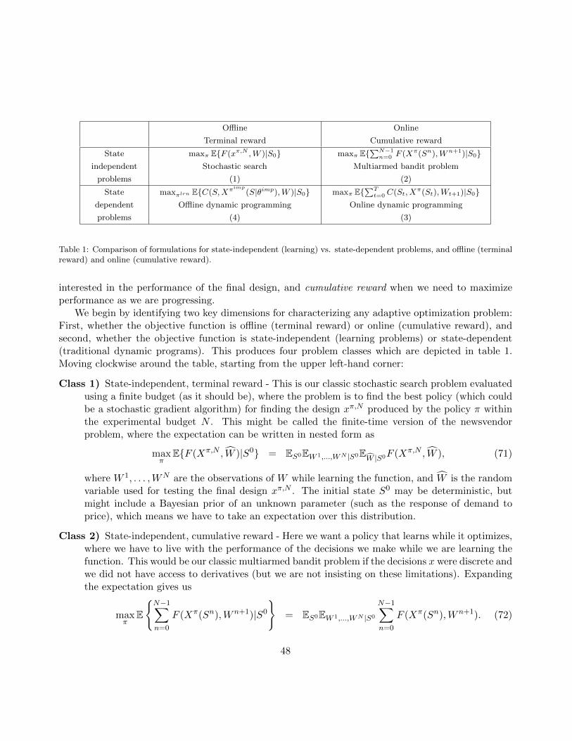
Offline

Terminal reward

Online

Cumulative reward

State

independent

problems

maxπ EF (xπ,N ,W )|S0Stochastic search

(1)

maxπ E∑N−1n=0 F (Xπ(Sn),Wn+1)|S0

Multiarmed bandit problem

(2)

State

dependent

problems

maxπlrn EC(S,Xπimp

(S|θimp),W )|S0Offline dynamic programming

(4)

maxπ E∑Tt=0 C(St, X

π(St),Wt+1)|S0Online dynamic programming

(3)

Table 1: Comparison of formulations for state-independent (learning) vs. state-dependent problems, and offline (terminalreward) and online (cumulative reward).

interested in the performance of the final design, and cumulative reward when we need to maximizeperformance as we are progressing.

We begin by identifying two key dimensions for characterizing any adaptive optimization problem:First, whether the objective function is offline (terminal reward) or online (cumulative reward), andsecond, whether the objective function is state-independent (learning problems) or state-dependent(traditional dynamic programs). This produces four problem classes which are depicted in table 1.Moving clockwise around the table, starting from the upper left-hand corner:

Class 1) State-independent, terminal reward - This is our classic stochastic search problem evaluatedusing a finite budget (as it should be), where the problem is to find the best policy (which couldbe a stochastic gradient algorithm) for finding the design xπ,N produced by the policy π withinthe experimental budget N . This might be called the finite-time version of the newsvendorproblem, where the expectation can be written in nested form as

maxπ

EF (Xπ,N , W )|S0 = ES0EW 1,...,WN |S0EW |S0F (Xπ,N , W ), (71)

where W 1, . . . ,WN are the observations of W while learning the function, and W is the randomvariable used for testing the final design xπ,N . The initial state S0 may be deterministic, butmight include a Bayesian prior of an unknown parameter (such as the response of demand toprice), which means we have to take an expectation over this distribution.

Class 2) State-independent, cumulative reward - Here we want a policy that learns while it optimizes,where we have to live with the performance of the decisions we make while we are learning thefunction. This would be our classic multiarmed bandit problem if the decisions x were discrete andwe did not have access to derivatives (but we are not insisting on these limitations). Expandingthe expectation gives us

maxπ

E

N−1∑n=0

F (Xπ(Sn),Wn+1)|S0

= ES0EW 1,...,WN |S0

N−1∑n=0

F (Xπ(Sn),Wn+1). (72)

48

Class 3) State-dependent, cumulative reward - At first glance this looks like a classical dynamicprogram (when expressed in terms of optimizing over policies), yet we see that it closely parallelsthe multiarmed bandit problem. This problem may include a belief state, but not necessarily.When we expand the expectation we obtain

maxπ

E

T−1∑t=0

C(St, Xπ(St),Wt+1)|S0

= ES0EW1,...,WT |S0

T−1∑t=0

C(St, Xπ(St),Wt+1)|S0

.

(73)

In contrast with problem classes (1) and (2), we model the performance of the policy over timet, rather than iterations n as we did in (72) (which could have been written either way).

Class 4) State-dependent, terminal reward - Here we are looking for the best policy to learn a policythat will then be implemented. Our implementation policy Xπimp(St|θimp) parallels the imple-

mentation decision xπ,N in (71), where θimp = Θπlrn(S|θlrn) is a parameter that is learned by the

learning policy Θπlrn(S|θlrn). The learning policy could be algorithms for learning value func-tions such as Q-learning, approximate value iteration or SDDP, or it could be a search algorithmfor learning a PFA or CFA. The parameters θimp are parameters that determine the behaviorof the implementation policy such as an approximate Q-factor Q(s, a), a Benders’ cut, or thetunable parameter in a UCB policy.

When we have a state-dependent function, we have to take an additional expectation over thestate variable when evaluating the policy. Keeping in mind that the implementation parametersθimp are a function of the learning policy πlrn, we can write this as

maxπlrn

EC(S,Xπimp(S|θimp), W )|S0 =

ES0Eπlrn

W 1,...,WN |S0Eπimp

S|S0Eπimp

W |S0C(S,Xπimp(S|θimp), W ). (74)

where W 1, . . . ,WN represents the observations made while using our budget of N experimentsto learn a policy, and W is the random variable observed when evaluating the policy at the end.

Computing the expectation EπimpS|S0 over the states is typically intractable because it depends on

the implementation policy (which of course depends on the learning policy). Instead, we can runa simulation over a horizon t = 0, . . . , T − 1 and then divide by T to get an average contributionper unit time. We can think of Wn as the set of realizations over a simulation, which we canwrite as Wn = (Wn

1 , . . . ,WnT ). We can then write our learning problem as

maxπlrn

ES0Eπimp

(Wnt )Tt=1,n=1,...,N |S0

(Eπ

imp

(Wt)Tt=1|S0

1

T

T−1∑t=0

C(St, Xπimp(St|θimp), Wt+1)

). (75)

Here, we are searching over learning policies, where the simulation over time replaces F (x,W ) inthe state-independent formulation. The sequence (Wn

t )Tt=1, n = 1, . . . , N replaces the sequence

49

W 1, . . . ,WN for the state-independent case, where we start at state S0 = S0. We then do ourfinal evaluation by taking an expectation over (Wt)

Tt=1, where we again assume we start our

simulations at S0 = S0.

This organization brings out relationships that have not been highlighted in the past. For example,while ranking and selection/stochastic search has been viewed as a fundamentally different problemclass from multiarmed bandits, we see that they are really the same problem with different objectives(final reward versus cumulative reward). We also see that state-independent problems (learning prob-lems) are closely related to state-dependent problems, which is the problem class typically associatedwith dynamic programming (although all of these problems are dynamic programs).

We have noted that most adaptive learning algorithms for dynamic programming (Q-learning,approximate dynamic programming, SDDP) fall under the category of state-dependent, final-rewardin table 1, which suggests that the cumulative-reward, state-dependent case is a relatively overlookedproblem class (excluding contextual bandits, which is a special case). Algorithms in this setting haveto balance learning while making good decisions (the classic exploration-exploitation tradeoff). Somecontributions to this problem class include the work of Duff (Duff et al. (1996) and Duff (2002)) whichtried to adapt the theory of Gittins indices to Q-learning algorithms, and Ryzhov (Ryzhov & Powell(2010) and Ryzhov et al. (2017)) who developed both offline (final reward) and online (cumulativereward) adaptations of the knowledge gradient algorithm for state-dependent problems.

There is a substantial literature that makes the distinction between problems in classes (1) and(2), primarily because optimal policies and their behavior (and hence, theoretical properties) are quitedifferent. By contrast, while there are communities doing (state dependent) dynamic programming inboth offline and online settings, the algorithms (policies) used for each setting are fundamentally thesame. Why is this? We believe it is because classes (1) and (2) are relatively simple, and lend themselvesto finding theoretical results characterizing the behavior of policies, where the slight differences between(1) and (2) are important. By contrast, if you are focusing on designing algorithms to find optimalpolicies, the distinction between the final reward and cumulative reward objective functions is simplynot that important. Imagine solving linear programs for deterministic versions of (3) and (4); thesimplex algorithm will solve both of these.

11. Research challenges

The framework presented here brings a variety of perspectives from the different communities ofstochastic optimization, which creates new opportunities for research. These include:

• Given the complexity of solving a stochastic lookahead model, most authors are happy just toget a solution. As a result, almost no attention has been devoted to analyzing the quality of astochastic lookahead model. We need more research to understand the impact of the differenttypes of errors that are introduced by the approximations discussed in section 5.2 when creatinglookahead models.

50

• There has been a long tradition of solving problems with belief states as “partially observableMarkov decision processes.” At the same time, theoreticians have known for decades that dy-namic programs with belief states can be modeled simply as part of the state variable (as wehave done), which means that POMDPs are really just dynamic programs which can be solvedwith any of the four classes of policies. In fact, we have described policies designed for problemswhere the state variable is purely a belief state. We need to explore the four classes of policies forproblems with mixed state variables (physical, informational, and belief), rather than assumingthat we have to always solve Bellman’s equation.

• The quality of a policy depends on the quality of a model; the stochastic optimization literatureputs relatively little attention into the model of uncertainty, although some attention has beengiven to the identification of suitable scenarios in a sampled model, and the design of distribu-tionally robust models. There is, of course, an extensive literature on stochastic modeling anduncertainty quantification; we need considerably more research at the intersection of these fieldsand stochastic optimization.

• Design of algorithms for online (cumulative reward) settings. The vast majority of adaptivesearch algorithms (stochastic gradient methods, Benders decomposition, Q-learning, approximatedynamic programming) are implemented in an offline context where the goal is to produce asolution that “works well.” There are many settings where learning has to be performed online,which means we have to do well as we are learning, which is the standard framework of multiarmedbandit problems. We can bring this thinking into classical stochastic search problems.

• All of the communities described in section 2 focus on expectation-based objectives, yet riskis almost always an issue in stochastic problems. There is a growing literature on the use ofrisk measures, but we feel that the current literature is only scratching the surface in terms ofaddressing computational and modeling issues in the context of specific applications.

• Parametric cost function approximations, particularly in the form of modified deterministic mod-els, are widely used in engineering practice (think of scheduling an airline with schedule slack tohandle uncertainty). This strategy represents a powerful alternative to stochastic programmingfor handling multistage stochastic math programs. We envision that this research will consist ofcomputational research to develop and test search algorithms for optimizing parametric CFAs,along with the theoretical analysis of structural results to guide the design of these policies.

• With rare exceptions, authors will pursue one of the four classes of policies we have describedabove, but it is not always obvious which is best, and it can depend on the characteristics ofthe data. We need a robust methodology that searches across classes of policies, and performsself-tuning, in an efficient way. Of course, we will always be searching for the ultimate functionthat replaces all four classes, but we are not optimistic that this will be possible in practice.

51

• Multiple objectives - Stochastic dynamic problems tend to be richer and more complex, and onebyproduct of this is that these problems are often multi-objective. At a minimum, we have tohandle risk and reward, but in real applications, there tend to be several important metrics thatare being managed.

• Multiple agents - A rich direction to extend this modeling framework is to include multiple agents.This raises issues of communication, coordination and adversarial behavior.

Each of these topics are deep and rich, and could represent entire fields of research.

Acknowledgements

This work was funded in part by AFOSR grant FA9550-12-1-0200, NSF grant CMMI-1537427 andDARPA grant FA8750-17-2-0027.

52

Aberdeen, D. (2003), ‘A (revised) survey of approximate methods for solving partially observableMarkov decision processes’, National ICT Australia, Canberra, Australia pp. 1–41.

Agrawal, S. & Goyal, N. (2012), Analysis of Thompson Sampling for the multi-armed bandit problem,in ‘Conference on Learning Theory (COLT)’, Association for Computational Learning, Edinburgh,pp. 1–21.

Albers, S. (2003), ‘Online Algorithms: A Survey’, Mathematical Programming 97(1-2), 3–26.

Andradottir, S. (1998a), ‘A review of simulation optimization techniques’, 1998 Winter SimulationConference. Proceedings 1(0), 151–158.

Andradottir, S. (1998b), Simulation Optimimzation, in J. Banks, ed., ‘Handbook of simulation’, JohnWiley & Sons, Hoboken, NJ, chapter 9, pp. 307–333.

Ankenman, B., Nelson, B. L. & Staum, J. (2010), ‘Stochastic Kriging for Simulation Metamodeling’,Operations Research 58(2), 371–382.

Asmussen, S. & Glynn, P. W. (2007), Stochastic simulation: algorithms and analysis, Springer Science& Business Media.

Astrom, K. J. (1970), Introduction to Stochastic Control Theory, Dover Publications, Mineola, NY.

Audibert, J.-y. & Bubeck, S. (2010), ‘Best Arm Identification in Multi-Armed Bandits’, CoLT p. 13 p.

Auger, D., Couetoux, A. & Teytaud, O. (2013), ‘Continuous upper confidence trees with polynomialexploration - Consistency’, Lecture Notes in Computer Science (including subseries Lecture Notesin Artificial Intelligence and Lecture Notes in Bioinformatics) 8188(PART 1), 194–209.

Azadivar, F. (1999), Simulation Optimization Methodologies, in P. Farrington, H. Nembhard, D. Stur-rock & G. Evans, eds, ‘Proceedings of the 1999 Winter Simulation Conference’, IEEE, pp. 93–100.

Azevedo, A. & Paxson, D. (2014), ‘Developing real option game models’, European Journal of Opera-tional Research 237(3), 909–920.

Banks, J., Nelson, B. L. & J. S. Carson, I. I. (1996), Discrete-Event System Simulation, Prentice-Hall,Inc., Englewood Cliffs, N.J.

Bartlett, P. L., Hazan, E. & Rakhlin, A. (2007), ‘Adaptive Online Gradient Descent’, Advances inneural information processing systems pp. 1–8.

Barut, E. & Powell, W. B. (2014), ‘Optimal learning for sequential sampling with non-parametricbeliefs’, J. Global Optimization 58, 517–543.

Bayraksan, G. & Love, D. K. (2015), ‘Data-Driven Stochastic Programming Using Phi- Divergences’,Informs TutORials in Operations Research 2014 pp. 1–19.

Bayraksan, G. & Morton, D. (2009), ‘Assessing solution quality via sampling in stochastic programs’,TutORials in Operations Research 514, 495–514.

53

Bayraksan, G. & Morton, D. P. (2011), ‘A Sequential Sampling Procedure for Stochastic Programming’,Operations Research 59(4), 898–913.

Bellman, R. E. (1954), ‘The Theory of Dynamic Programming’, Bull. Amer. Math. Soc. 60, 503–516.

Bellman, R. E. (1957), Dynamic Programming, Princeton University Press, Princeton, N.J.

Bellman, R. E. & Dreyfus, S. E. (1959), ‘Functional approximations and dynamic programming’,Mathematical Tables and Other Aids to Computation 13, 247–251.

Bellman, R. E., Glicksberg, I. & Gross, O. (1955), ‘On the Optimal Inventory Equation’, ManagementScience 1, 83–104.

Bellman, R., Kalaba, R. & Kotkin, B. (1963), ‘Polynomial approximation— a new computationaltechnique in dynamic programming: Allocation processes’, Mathematics of Computation 17, 155–161.

Ben-Tal, A., El Ghaoui, L. & Nemirovski, A. (2009), ‘Robust Optimization’, Princeton UniversityPress 53(3), 464–501.

Ben-Tal, A., Golany, B., Nemirovski, A. & Vial, J.-p. (2005), ‘Retailer-Supplier Flexible CommitmentsContracts: A Robust Optimization Approach’, Manufacturing & Service Operations Management7(3), 248–271.

Berbeglia, G., Cordeau, J. F. & Laporte, G. (2010), ‘Dynamic pickup and delivery problems’, EuropeanJournal of Operational Research 202(1), 8–15.

Bertsekas, D. (2005), ‘Dynamic programming and suboptimal control: A survey from ADP to MPC’,European Journal of Control 11(4-5), 310—-334.

Bertsekas, D. P. (2011), Dynamic Programming and Optimal Control, Vol. II: Approximate DynamicProgramming, 4 edn, Athena Scientific, Belmont, MA.

Bertsekas, D. P. & Castanon, D. A. (1999), ‘Rollout Algorithms for Stochastic Scheduling Problems’,J. Heuristics 5, 89–108.

Bertsekas, D. P. & Shreve, S. E. (1978), Stochastic optimal control: the discrete time case, Vol. 0,Academic Press.

Bertsekas, D. P. & Tsitsiklis, J. N. (1996), Neuro-Dynamic Programming, Athena Scientific, Belmont,MA.

Bertsimas, D., Brown, D. B. & Caramanis, C. (2011), ‘Theory and applications of robust optimization’,SIAM Review 53(3), 464–501.

Bertsimas, D. J. & Sim, M. (2004), ‘The Price of Robustness’, Operations Research 52(1), 35–53.

Bertsimas, D. J. & Thiele, A. (2006), ‘A Robust Optimization Approach to Inventory Theory’, Oper-ations Research 54(1), 150–168.

Birge, J. R. & Louveaux, F. (2011), Introduction to Stochastic Programming, 2nd edn, Springer, NewYork.

54

Blum, J. (1954), ‘Multidimensional stochastic approximation methods’’, Annals of Mathematical Statis-tics 25, 737–74462.

Boomsma, T. K., Meade, N. & Fleten, S. E. (2012), ‘Renewable energy investments under differentsupport schemes: A real options approach’, European Journal of Operational Research 220(1), 225–237.

Borodin, A. & El-Yanniv, R. (1998), Online Computation and Competitive Analysis, Cambridge UnivPress, London.

Bouzaiene-Ayari, B., Cheng, C., Das, S., Fiorillo, R. & Powell, W. B. (2014), ‘From Single Com-modity to Multiattribute Models for Locomotive Optimization : A Comparison of Optimal IntegerProgramming and Approximate Dynamic Programming’, Transportation Science pp. 1–24.

Bouzaiene-Ayari, B., Cheng, C., Das, S., Fiorillo, R. & Powell, W. B. (2016), ‘From single commodityto multiattribute models for locomotive optimization: A comparison of optimal integer programmingand approximate dynamic programming’, Transportation Science.

Broadie, M., Cicek, D. & Zeevi, a. (2011), ‘General Bounds and Finite-Time Improvement for theKiefer-Wolfowitz Stochastic Approximation Algorithm’, Operations Research 59(5), 1211–1224.

Browne, C. B., Powley, E., Whitehouse, D., Lucas, S. M., Cowling, P. I., Rohlfshagen, P., Tavener, S.,Perez, D., Samothrakis, S. & Colton, S. (2012), ‘A Survey of Monte Carlo Tree Search Methods’,IEEE Trans. on Computational Intelligence and AI in Games 4(1), 1–43.

Bubeck, S. & Cesa-Bianchi, N. (2012), ‘Regret Analysis of Stochastic and Nonstochastic Multi-armedBandit Problems’, Foundations and Trends in Machine Learning 5(1), 1–122.

Busoniu, L., Babuska, R., De Schutter, B. & Ernst, D. (2010), Reinforcement Learning and DynamicProgramming using Function Approximators, CRC Press, New York.

Camacho, E. & Bordons, C. (2003), Model Predictive Control, Springer, London.

Cassandra, A. R., Kaelbling, L. P. & Littman, M. L. (1994), Acting Optimally in Partially ObservableStochastic Domains, in ‘AAAI’, pp. 1–6.

Chau, M., Fu, M. C., Qu, H. & Ryzhov, I. O. (2014), Simulation Optimization: A Tutorial Overviewand Recent Developments in Gradient-Based Methods, in A. Tolk, S. Diallo, I. Ryzhov, L. Yilmaz,S. Buckley & J. Miller, eds, ‘Winter Simulation Conference’, Informs, pp. 21–35.

Chen, C. H. (1995), An effective approach to smartly allocate computing budget for discrete eventsimulation, in ‘34th IEEE Conference on Decision and Control’, Vol. 34, New Orleans, LA, pp. 2598–2603.

Chen, C. H. (1996), ‘A lower bound for the correct subset-selection probability and its application todiscrete event system simulations. IEEE Transactions on’, Automatic Control 41(8), 1227–1231.

Chen, C.-H. & Lee, L. H. (2011), Stochastic Simulation Optimization, World Scientific Publishing Co.,Hackensack, N.J.

55

Chen, C. H., Donohue, K., Yucesan, E. & Lin, J. (2003), ‘Optimal computing budget allocation forMonte Carlo simulation with application to product design’, Simulation Modelling Practice andTheory 11, 57–74.

Chen, C. H., He, D., Fu, M. C. & Lee, L. H. (2008), ‘Efficient simulation budget allocation for selectingan optimal subset’, INFORMS Journal on Computing 20(4), 579–595.

Chen, C. H., Yuan, Y., Chen, H. C., Yucesan, E. & Dai, L. (1998), Computing budget allocation forsimulation experiments with different system structure, in ‘Proceedings of the 30th conference onWinter simulation’, pp. 735–742.

Chen, H. C., Chen, C. H., Dai, L. & Yucesan, E. (1997), A gradient approach for smartly allocatingcomputing budget for discrete event simulation, in J. Charnes, D. Morrice, D. Brunner & J. Swain,eds, ‘Proceedings of the 1996 Winter Simulation Conference’, IEEE Press, Piscataway, NJ, USA,pp. 398–405.

Chen, S., Reyes, K.-R. G., Gupta, M., Mcalpine, M. C. & Powell, W. B. (2015), ‘Optimal learningin Experimental Design Using the Knowledge Gradient Policy with Application to CharacterizingNanoemulsion Stability’, SIAM/ASA J. Uncertainty Quantification 3, 320–345.

Chen, V. C. P., Ruppert, D. & Shoemaker, C. A. (1999), ‘Applying experimental design and regressionsplines to high-dimensional continuous-state stochastic dynamic programming’, Operations Research47(1), 38–53.

Cheng, B., Asamov, T. & Powell, W. B. (2017), ‘Low-Rank Value Function Approximation for Co-optimization of Battery Storage’, IEEE Transactions on Smart Grid.

Cheng, B., Jamshidi, A. & Powell, W. B. (2014), ‘Optimal Learning with a Local Parametric BeliefModel’, (2006), 1–37.

Chick, S. E. & Gans, N. (2009), ‘Economic Analysis of Simulation Selection Problems’, ManagementScience 55(3), 421–437.

Chick, S. E., Branke, J. & Schmidt, C. (2010), ‘Sequential sampling to myopically maximize theexpected value of information’, INFORMS Journal on Computing 22(1), 71–80.

Cinlar, E. (1975), Introduction to Stochastic Processes, Prentice Hall, Upper Saddle River, NJ.

Cinlar, E. (2011), Probability and Stochastics, Springer, New York.

Collado, R. A., Papp, D. & Ruszczynski, A. (2011), ‘Scenario decomposition of risk-averse multistagestochastic programming problems’, Annals of Operations Research 200(1), 147–170.

Cressie, N. (1990), ‘The origins of kriging’, Mathematical Geology 22(3), 239–252.

Dantzig, G. B. (1955), ‘Linear programming with uncertainty’, Management Science 1, 197–206.

Dantzig, G. B. & Ferguson, A. (1956), ‘The Allocation of Aircrafts to Routes: An Example of LinearProgramming Under Uncertain Demand’, Management Science 3, 45–73.

56

Defourny, B., Ernst, D. & Wehenkel, L. (2013), ‘Scenario Trees and Policy Selection for MultistageStochastic Programming using Machine Learning’, Informs J. on Computing pp. 1–27.

DeGroot, M. H. (1970), Optimal Statistical Decisions, John Wiley and Sons.

Denardo, E. V. (1982), Dynamic Programming, Prentice-Hall, Englewood Cliffs, NJ.

Duchi, J., Hazan, E. & Singer, Y. (2011), ‘Adaptive Subgradient Methods for Online Learning andStochastic Optimization’, Journal of Machine Learning Research 12, 2121–2159.

Duff, M. O. (2002), ‘Optimal Learning: Computational Procedures for Bayes-Adaptive Markov Deci-sion Processes’.

Duff, M. O., Barto, A. G. & Du, M. O. (1996), Local bandit approximation for optimal learningproblems, in M. C. Mozer, M. I. Jordan & T. Petsche, eds, ‘Proceedings of the 9th InternationalConference on Neural Information Processing Systems’, Department of Computer Science, Universityof Massachusetts, MIT Press, Cambridge, MA, pp. 1019–1025.

Dupacova, J., Growe-Kuska, N. & Romisch, W. (2003), ‘Scenario reduction in stochastic programming:An approach using probability metrics’, Math. Program., Ser. A 95, 493511.

Durante, J. L., Nascimento, J. & Powell, W. B. (2017), Backward Approximate Dynamic Programmingwith Hidden Semi-Markov Stochastic Models in Energy Storage Optimization, Technical report,Princeton University, Princeton NJ.

Dvoretzky, A. (1956), On Stochastic Approximation, in J. Neyman, ed., ‘Proceedings 3rd BerkeleySymposium on Mathematical Statistics and Probability’, University of California Press, pp. 39–55.

Ermoliev, Y. (1968), ‘On the stochastic quasi-gradient methods and stochastic quasi-Feyer sequence’,Kibernetika.

Feng, Y. & Gallego, G. (1995), ‘Optimal Starting Times for End-of-Season Sales and Optimal StoppingTimes for Promotional Fares’, Management Science 41(8), 1371–1391.

Fliege, J. & Werner, R. (2014), ‘Robust multiobjective optimization and applications in portfoliooptimization’, European Journal of Operational Research 234(2), 422–433.

Frazier, P. I. & Powell, W. B. (2010), ‘Paradoxes in Learning and the Marginal Value of Information’,Decision Analysis 7(4), 378–403.

Frazier, P. I., Powell, W. B. & Dayanik, S. (2008), ‘A knowledge gradient policy for sequential infor-mation collection’, SIAM Journal on Control and Optimization 47(5), 2410–2439.

Frazier, P. I., Powell, W. B. & Dayanik, S. (2009), ‘The Knowledge-Gradient Policy for CorrelatedNormal Beliefs’, INFORMS Journal on Computing 21(4), 599–613.

Fu, M. C. (2002), ‘Optimization for simulation: Theory vs. practice’, Informs Journal on Computing14(3), 192–215.

Fu, M. C. (2014), Handbook of Simulation Optimization, Springer, New York.

57

Gabillon, V., Ghavamzadeh, M. & Lazaric, A. (2012), ‘Best arm identification: A unified approach tofixed budget and fixed confidence’, Nips pp. 1–9.

Gabrel, V., Murat, C. & Thiele, A. (2014), ‘Recent advances in robust optimization: An overview’,European Journal of Operational Research 235(3), 471–483.

Ginebra, J. & Clayton, M. K. (1995), ‘Response Surface Bandits’, Journal of the Royal StatisticalSociety. Series B (Methodological) 57(4), 771–784.

Girardeau, P., Leclere, V. & Philpott, A. B. (2014), ‘On the Convergence of Decomposition Methodsfor Multistage Stochastic Convex Programs’, Mathematics of Operations Research 40(1), 130–145.

Gittins, J. (1979), ‘Bandit processes and dynamic allocation indices’, Journal of the Royal StatisticalSociety. Series B (Methodological) 41(2), 148–177.

Gittins, J. (1989), ‘Multi-armed Bandit Allocation Indices’, Wiley and Sons: New York.

Gittins, J. & Jones, D. (1974), A dynamic allocation index for the sequential design of experiments,in J. Gani, ed., ‘Progress in statistics’, North Holland, Amsterdam, pp. 241—-266.

Gittins, J., Glazebrook, K. D. & Weber, R. R. (2011), Multi-Armed Bandit Allocation Indices, JohnWiley & Sons, New York.

Goh, J. & Sim, M. (2010), ‘Distributionally robust optimization and its tractable approximations’,Operations Research 58(4, Part 1 of 2), 902–917.

Hagspiel, V., Huisman, K. J. & Nunes, C. (2015), ‘Optimal technology adoption when the arrival rateof new technologies changes’, European Journal of Operational Research 243(3), 897–911.

Hastie, T. J., Tibshirani, R. J. & Friedman, J. H. (2009), The elements of statistical learning : datamining, inference, and prediction, Springer, New York.

Heitsch, H. & Romisch, W. (2009), ‘Scenario tree modeling for multistage stochastic programs’, Math-ematical Programming 118, 371–406.

Heyman, D. P. & Sobel, M. (1984), Stochastic Models in Operations Research, Volume II: StochasticOptimization, McGraw Hill, New York.

Higle, J. L. & Sen, S. (1991), ‘Stochastic decomposition: An algorithm for two-stage linear programswith recourse’, Mathematics of Operations Research 16(3), 650–669.

Hong, J. & Nelson, B. L. (2006), ‘Discrete Optimization via Simulation Using COMPASS’, OperationsResearch 54(1), 115–129.

Howard, R. A. (1960), Dynamic programming and Markov processes, MIT Press, Cambridge, MA.

Infanger, G. & Morton, D. P. (1996), ‘Cut Sharing for Multistage Stochastic Linear Programs withInterstage Dependency’, Mathematical Programming 75, 241–256.

58

Ivanov, D. & Sokolov, B. (2013), ‘Control and system-theoretic identification of the supply chaindynamics domain for planning, analysis and adaptation of performance under uncertainty’, EuropeanJournal of Operational Research 224(2), 313–323.

Jaakkola, T., Jordan, M. I. & Singh, S. P. (1994), ‘On the Convergence of Stochastic Iterative DynamicProgramming Algorithms’, Neural Computation 6, 1185—-1201.

Jaillet, P. & Wagner, M. R. (2006), ‘Online Routing Problems: Value of Advanced Information asImproved Competitive Ratios’, Transportation Science 40(2), 200–210.

Jiang, D. R. & Powell, W. B. (2016a), Optimal Policies for Risk-Averse Electric Vehicle Charging withSpot Purchases.

Jiang, D. R. & Powell, W. B. (2016b), Risk-averse approximate dynamic programming with quantile-based risk measures, Technical report.

Jiang, D. R., Al-Kanj, L. & Powell, W. B. (2017), Monte Carlo Tree Search with Sampled InformationRelaxation Dual Bounds, Technical report, University of Pittsburgh, Pittsburgh, PA.

Jones, D. R. (2001), ‘A Taxonomy of Global Optimization Methods Based on Response Surfaces’,Journal of Global Optimization pp. 345–383.

Jones, D., Schonlau, M. & Welch, W. (1998), ‘Efficient global optimization of expensive black-boxfunctions’, Journal of Global Optimization 13(4), 455—-492.

Judd, K. L. (1998), Numerical Methods in Economics, MIT Press.

Kaelbling, L. P., Littman, M. L. & Moore, A. W. (1996), ‘Reinforcement learning: a survey’, J. Artif.Intell. Res. 4, 237–285.

Kall, P. & Wallace, S. (2009), Stochastic Programming, Vol. 10, John Wiley & Sons, Hoboken, NJ.

Karatzas, I. (1988), ‘On the pricing of American options’, Applied Mathematics and Optimization17(1), 37–60.

Kaufmann, E., Cappe, O. & Garivier, A. (2016), ‘On the Complexity of Best-Arm Identification inMulti-Armed Bandit Models’, Journal of Machine Learning Research 17, 1–42.

Kesten, H. (1958), ‘Accelerated Stochastic Approximation’, The Annals of Mathematical Statistics29, 41–59.

Keyvanshokooh, E., Ryan, S. M. & Kabir, E. (2016), ‘Hybrid robust and stochastic optimization forclosed-loop supply chain network design using accelerated Benders decomposition’, European Journalof Operational Research 249(1), 76–92.

Kim, S.-H. & Nelson, B. L. (2007), Recent advances in ranking and selection, IEEE Press, Piscataway,NJ, USA, pp. 162–172.

King, A. J. & Wallace, S. W. (2012), Modeling with Stochastic Programming, Springer Verlag, NewYork.

59

Kingma, D. P. & Ba, J. L. (2015), Adam: a Method for Stochastic Optimization, in ‘InternationalConference on Learning Representations 2015’, pp. 1–15.

Kirk, D. E. (2004), Optimal Control Theory: An introduction, Dover, New York.

Kleijnen, J. P. (2014), ‘Simulation-optimization via Kriging and bootstrapping: a survey’, Journal ofSimulation 8(4), 241–250.

Kleijnen, J. P. (2017), ‘Regression and Kriging metamodels with their experimental designs in simula-tion: A review’, European Journal of Operational Research 256(1), 1–16.

Kleywegt, A. J., Shapiro, A. & Homem-de Mello, T. (2002), ‘The Sample Average ApproximationMethod for Stochastic Discrete Optimization’, SIAM Journal on Optimization 12(2), 479–502.

Kozmık, V. & Morton, D. P. (2014), ‘Evaluating policies in risk-averse multi-stage stochastic program-ming’, Mathematical Programming 152(1-2), 275–300.

Kupper, M. & Schachermayer, W. (2009), ‘Representation results for law invariant time consistentfunctions’, Mathematics and Financial Economics 2(3), 189–210.

Kushner, H. J. & Clark, S. (1978), Stochastic Approximation Methods for Constrained and Uncon-strained Systems, Springer-Verlag, New York.

Kushner, H. J. & Kleinman, A. J. (1971), ‘Accelerated Procedures for the Solution of Discrete MarkovControl Problems’, IEEE Transactions on Automatic Control 16, –2147–152.

Kushner, H. J. & Yin, G. G. (2003), Stochastic Approximation and Recursive Algorithms and Appli-cations, Springer, New York.

Lai, T. L. & Robbins, H. (1985), ‘Asymptotically efficient adaptive allocation rules’, Advances inApplied Mathematics 6(1), 4–22.

Lee, J. H. (2011), ‘Model predictive control: Review of the three decades of development’, InternationalJournal of Control, Automation and Systems 9(3), 415–424.

Lewis, F. L., Vrabie, D. & Syrmos, V. L. (2012), Optimal Control, 3rd edn, John Wiley & Sons,Hoboken, NJ.

Lohndorf, N. (2016), ‘An empirical analysis of scenario generation methods for stochastic optimization’,European Journal of Operational Research 255(1), 121–132.

Longstaff, F. A. & Schwartz, E. S. (2001), ‘Valuing American options by simulation: A simple leastsquares approach’, The Review of Financial Studies 14(1), 113–147.

Lovejoy, W. S. (1991), ‘A survey of algorithmic methods for partially observed Markov decision pro-cesses’, Annals of Operations Research 28(1), 47–651.

Luo, J., Hong, L. J., Nelson, B. L. & Wu, Y. (2015), ‘Fully Sequential Procedures for Large-Scale Ranking-and-Selection Problems in Parallel Computing Environments’, Operations Research63(5), 1177–1194.

60

Ma, Y., Chu, C. & Zuo, C. (2010), ‘A survey of scheduling with deterministic machine availabilityconstraints’, Computers and Industrial Engineering 58(2), 199–211.

Mes, M. R. K., Powell, W. B. & Frazier, P. I. (2011), ‘Hierarchical Knowledge Gradient for SequentialSampling’, Journal of Machine Learning Research 12, 2931–2974.

Moazeni, S., Powell, W. B., Defourny, B. & Bouzaiene-ayari, B. (2017), ‘Parallel Nonstationary DirectPolicy Search for Risk-Averse Stochastic Optimization’, Informs J. on Computing 29(2), 332–349.

Montgomery, D. (2000), Design and Analysis of Experiments, John Wiley & Sons Inc.

Morari, M., Lee, J. H. & Garc, C. E. (2002), Model Predictive Control, Springer-Verlag, New York.

Moustakides, G. V. . (1986), ‘Optimal Stopping Times for Detecting Changes in Distributions’, Annalsof Statistics 14(4), 1379–1387.

Munos, R. (2014), ‘From Bandits to Monte-Carlo Tree Search: The Optimistic Principle Applied toOptimization and Planning’, Foundations and Trends R© in Machine Learning 7(1), 1–129.

Negoescu, D. M., Frazier, P. I. & Powell, W. B. (2010), ‘The Knowledge-Gradient Algorithm forSequencing Experiments in Drug Discovery’, INFORMS Journal on Computing pp. 1–18.

Nemhauser, G. L. (1966), Introduction to dynamic programming, John Wiley & Sons, New York.

Ni, E. C., Henderson, S. G. & Hunter, S. R. (2016), ‘Efficient Ranking and Selection in ParallelComputing Environments’, Operations Research 65(3), 821–836.

Nisio, M. (2014), Stochastic Control Theory: Dynamic Programming Principle, Springer, New York.

Oliehoek, F. A., Spaan, M. T. & Vlassis, N. (2008), ‘Optimal and approximate Q-value functions fordecentralized POMDPs’, Journal of Artificial Intelligence Research 32, 289–353.

Orabona, F. (2014), Simultaneous model selection and optimization through parameter-free stochasticlearning, in ‘Advances in Neural Information Processing Systems’, pp. 1–9.

Pereira, M. F. & Pinto, L. M. V. G. (1991), ‘Multi-stage stochastic optimization applied to energyplanning’, Mathematical Programming 52, 359–375.

Perkins, R. T. & Powell, W. B. (2017), Stochastic Optimization with Parametric Cost FunctionApproximations.

Pflug, G. (1988a), Numerical Methods in Stochastic Programming, Springer-Verlag.

Pflug, G. (1988b), Stepsize rules, stopping times and their implementation in stochastic quasi-gradientalgorithms, in ‘Numerical Techniques for Stochastic Optimization’, Springer-Verlag, New York,pp. 353–372.

Philpott, A. B. & de Matos, V. (2012), ‘Dynamic sampling algorithms for multi-stage stochasticprograms with risk aversion’, European Journal of Operational Research 218(2), 470–483.

61

Philpott, A. B., De Matos, V. & Finardi, E. (2013), ‘On Solving Multistage Stochastic Programs withCoherent Risk Measures’, Operations Research 51(4), 957–970.

Pillac, V., Gendreau, M., Gueret, C. & Medaglia, A. L. (2013), ‘A review of dynamic vehicle routingproblems’, European Journal of Operational Research 225(1), 1–11.

Pineau, J., Gordon, G. & Thrun, S. (2003), Point-based value iteration: An anytime algorithm forPOMDPs, in ‘IJCAI International Joint Conference on Artificial Intelligence’, pp. 1025–1030.

Poor, H. V. & Hadjiliadis, O. (2009), Quickest Detection, Cambridge University Press, Cambridge,U.K.

Powell, W. B. (2007), ‘Approximate Dynamic Programming: Solving the curses of dimensionality’.

Powell, W. B. (2011), Approximate Dynamic Programming: Solving the curses of dimensionality, 2edn, John Wiley & Sons, Hoboken, NJ.

Powell, W. B. (2014), ‘Clearing the Jungle of Stochastic Optimization’, Bridging Data and Decisions(January 2015), 109–137.

Powell, W. B. (2016), A Unified Framework for Optimization under Uncertainty.

Powell, W. B. & George, A. P. (2006), ‘Adaptive stepsizes for recursive estimation with applicationsin approximate dynamic programming’, Journal of Machine Learning 65(1), 167–198.

Powell, W. B. & Meisel, S. (2016a), ‘Tutorial on Stochastic Optimization in Energy - Part II: AnEnergy Storage Illustration’, IEEE Transactions on Power Systems.

Powell, W. B. & Meisel, S. (2016b), ‘Tutorial on Stochastic Optimization in Energy II: An energystorage illustration’, IEEE Transactions on Power Systems 31(2), 1459–1467.

Powell, W. B. & Ryzhov, I. O. (2012), Optimal Learning, John Wiley & Sons, Hoboken, NJ.

Powell, W. B., Ruszczynski, A. & Topaloglu, H. (2004), ‘Learning algorithms for separable approxima-tions of discrete stochastic optimization problems’, Math. Oper. Res. 29(4), 814–836.

Protopappa-Sieke, M. & Seifert, R. W. (2010), ‘Interrelating operational and financial performancemeasurements in inventory control’, European Journal of Operational Research 204(3), 439–448.

Puterman, M. (2005), Markov Decision Processes, 2nd edn, John Wiley & Sons Inc, Hoboken, NJ.

Qu, H., Ryzhov, I. O. & Fu, M. C. (2012), Ranking and selection with unknown correlation structures,in A. U. C. Laroque, J. Himmelspach, R. Pasupathy, O. Rose, ed., ‘Proceedings - Winter SimulationConference’, number 1995.

Ramirez-Nafarrate, A., Baykal Hafizoglu, A., Gel, E. S. & Fowler, J. W. (2014), ‘Optimal controlpolicies for ambulance diversion’, European Journal of Operational Research 236(1), 298–312.

Robbins, H. & Monro, S. (1951), ‘A stochastic approximation method’, The Annals of MathematicalStatistics 22(3), 400–407.

62

Rockafellar, R. T. & Uryasev, S. (2000), ‘Optimization of conditional value-at-risk’, Journal of Risk2, 21–41.

Rockafellar, R. T. & Uryasev, S. (2002), ‘Conditional value-at-risk for general loss distributions’,Journal of Banking & Finance 26, 1443–1471.

Rockafellar, R. T. & Uryasev, S. (2013), ‘The fundamental risk quadrangle in risk management, op-timization, and statistical estimation’, Surveys in Operations Research and Management Science18(1), 33–53.

Rockafellar, R. T. & Wets, R. J.-B. (1991), ‘Scenarios and policy aggregation in optimization underuncertainty’, Mathematics of Operations Research 16(1), 119–147.

Ross, S. M. (2002), Simulation, Academic Press, New York.

Ross, S., Pineau, J. & Chaib-Draa, B. (2008a), ‘Theoretical Analysis of Heuristic Search Methods forOnline POMDPs.’, NIPS 20, 1216–1225.

Ross, S., Pineau, J., Paquet, S. & Chaib-draa, B. (2008b), ‘Online planning algorithms for POMDPs’,Journal of Artificial Intelligence Research 32, 663–704.

Rubinstein, R. Y. & Kroese, D. P. (2017), Simulation and the Monte Carlo Method, 3rd edn, JohnWiley & Sons, Hoboken, NJ.

Russo, D. & Van Roy, B. (2014), ‘Learning to Optimize via Posterior Sampling’, Mathematics ofOperations Research 39(4), 1221–1243.

Ruszczynski, A. (2014), Advances in Risk-Averse Optimization, in ‘INFORMS Tutorials in OperationsResearch’, INFORMS, Baltimore, MD, pp. 168–190.

Ruszczynski, A. & Shapiro, A. (2006), ‘Optimization of Convex Risk Functions’, Mathematics ofOperations Research 31(3), 433–452.

Ryzhov, I. O. (2016), ‘On the Convergence Rates of Expected Improvement Methods’, OperationsResearch 64(6), 1515–1528.

Ryzhov, I. O. & Powell, W. B. (2010), Approximate Dynamic Programming With Correlated BayesianBeliefs, in ‘Forty-Eighth Annual Allerton Conference on Communication, Control, and Computing’,Monticello, IL.

Ryzhov, I. O., Mes, M. R. K., Powell, W. B. & van den Berg, G. A. (2017), Bayesian explorationstrategies for approximate dynamic programming, Technical report, University of Maryland, CollegePark.

Salas, D. & Powell, W. B. (2015), ‘Benchmarking a Scalable Approximate Dynamic ProgrammingAlgorithm for Stochastic Control of Multidimensional Energy Storage Problems’, Informs J. onComputing pp. 1–41.

Schildbach, G. & Morari, M. (2016), ‘Scenario-based model predictive control for multi-echelon supplychain management’, European Journal of Operational Research 252(2), 540–549.

63

Sen, S. & Zhou, Z. (2014), ‘Multistage stochastic decomposition: A bridge between stochastic pro-gramming and approximate dynamic programming’, SIAM J. Optimization 24(1), 127–153.

Senn, M., Link, N., Pollak, J. & Lee, J. H. (2014), ‘Reducing the computational effort of optimalprocess controllers for continuous state spaces by using incremental learning and post-decision stateformulations’, J. of Process Control2 24, 133–143.

Sethi, S. P. & Thompson, G. L. (2000), Optimal Control Theory, 2 edn, Kluwer Academic Publishers,Boston.

Shani, G., Pineau, J. & Kaplow, R. (2013), ‘A survey of point-based POMDP solvers’, AutonomousAgents and Multi-Agent Systems 27(1), 1–51.

Shapiro, A. (2011), ‘Analysis of stochastic dual dynamic programming method’, European Journal ofOperational Research 209(1), 63–72.

Shapiro, A. (2012), ‘Minimax and risk averse multistage stochastic programming’, European Journalof Operational Research 219(3), 719–726.

Shapiro, A. & Wardi, Y. (1996), ‘Convergence Analysis of Stochastic Algorithms’, Mathematics ofOperations Research 21, 615–628.

Shapiro, A., Dentcheva, D. & Ruszczynski, A. (2014), Lectures on Stochastic Programming: Modelingand theory, 2 edn, SIAM, Philadelphia.

Shapiro, A., Tekaya, W., Da Costa, J. P. & Soares, M. P. (2013), ‘Risk neutral and risk averse StochasticDual Dynamic Programming method’, European Journal of Operational Research 224(2), 375–391.

Sherif, Y. S. & Smith, M. L. (1981), ‘Optimal maintenance models for systems subject to failureAReview’, Naval Reseach Logistics Quarterly 28(1), 47–74.

Shiryaev, A. N. (1978), Optimal Stopping Rules, Springer, Moscow.

Shor, N. K. (1979), The Methods of Nondifferentiable Op[timization and their Applications, NaukovaDumka, Kiev.

Si, J., Barto, A. G., Powell, W. B. & Wunsch, D. (2004), ‘Handbook of learning and approximatedynamic programming’, Wiley-IEEE Press.

Simao, H. P., Day, J., George, A. P., Gifford, T., Powell, W. B. & Nienow, J. (2009), ‘An Approx-imate Dynamic Programming Algorithm for Large-Scale Fleet Management: A Case Application’,Transportation Science 43(2), 178–197.

Skinner, D. C. (1999), Introduction to Decision Analysis, Probabilistic Publishing, Gainesville, Fl.

Slotnick, S. A. (2011), ‘Order acceptance and scheduling: A taxonomy and review’, European Journalof Operational Research 212(1), 1–11.

Smallwood, R. D., Sondik, E. J. & Oct, N. S. (1973), ‘The Optimal Control of Partially ObservableMarkov Processes Over a Finite Horizon’, Operations Research 21(5), 1071–1088.

64

Smith, R. C. (2014), Uncertainty Quantification: Theory, Implementation, and Applications, SIAM,Philadelphia.

Smith, T. & Simmons, R. (2005), Point-Based POMDP Algorithms: Improved Analysis and Imple-mentation, in ‘Uai’, pp. 542–549.

Sondik, E. J. (1971), The optimal control of partially observable Markov decision processes, PhD thesis,Stanford University.

Sondik, E. J. (1978), ‘The Optimal Control of Partially Observable Markov Processes over the InfiniteHorizon: Discounted Costs’, Operations Research 26(2), 282–304.

Sontag, E. (1998), ‘Mathematical Control Theory, 2nd ed.’, Springer pp. 1–544.

Spall, J. C. (2003), Introduction to Stochastic Search and Optimization: Estimation, simulation andcontrol, John Wiley & Sons, Hoboken, NJ.

Stein, M. L. (1999), Interpolation of spatial data: Some theory for kriging, Springer Verlag, New York.

Stengel, R. F. (1986), Stochastic optimal control: theory and application, John Wiley & Sons, Hoboken,NJ.

Sullivan, T. (2015), Introduction to Uncertainty Quantification, Springer, New York.

Sutton, R. S. & Barto, A. G. (1998), Reinforcement Learning, MIT Press, Cambridge, MA.

Swisher, J. R., Hyden, P. D. & Schruben, L. W. (2000), ‘A survey of simulation optimization techniquesand procedures - Simulation Conference Proceedings, 2000. Winter’, pp. 119–128.

Szepesvari, C. (2010), Algorithms for Reinforcement Learning, Morgan and Claypool.

Thompson, W. R. (1933), ‘On the Likelihood that One Unknown Probability Exceeds Another in Viewof the Evidence of Two Samples’, Biometrika 25(3/4), 285–294.

Topaloglu, H. & Powell, W. B. (2006), ‘Dynamic Programming Approximations for Stochastic, Time-Staged Integer Multicommodity Flow Problems’, Informs Journal on Computing 18(1), 31–42.

Tsitsiklis, J. & Van Roy, B. (2001), ‘Regression methods for pricing complex American-style options’,IEEE Transactions on Neural Networks 12(4), 694–703.

Tsitsiklis, J. N. (1994), ‘Asynchronous stochastic approximation and Q-learning’, Machine Learning16, 185–202.

Van Slyke, R. M. & Wets, R. J.-B. (1969), ‘L-shaped linear programs with applications to optimalcontrol and stochastic programming’, SIAM Journal of Applied Mathematics 17, 638–663.

Werbos, P. J. (1974), Beyond regression: new tools for prediction and analysis in the behavioralsciences, PhD thesis, Harvard University.

Werbos, P. J. (1989), Backpropagation and neurocontrol: A review and prospectus, in ‘IJCNN, Inter-national Joint Conference on Neural Networks’, pp. 209—-216.

65

Werbos, P. J. (1990), ‘Backpropagation Through Time: What It Does and How to Do It’, Proceedingsof the IEEE 78(10), 1550–1560.

Werbos, P. J. (1992), Approximate Dynamic Programming for Real-Time Control and Neural Mod-elling, in D. J. White & D. A. Sofge, eds, ‘Handbook of Intelligent Control: Neural, Fuzzy, andAdaptive Approaches’.

Werbos, P. J. (1994), The Roots of Backpropagation: From Ordered Derivatives to Neural Networksand Political Forecasting, John Wiley & Sons, New York.

White, D. & Sofge, D. (1992), Handbook of intelligent control: Neural, fuzzy, and adaptive approaches,Van Nostrand Reinhold Company, New York.

Wiesemann, W., Kuhn, D. & Sim, M. (2014), ‘Distributionally Robust Convex Optimization’, Opera-tions Research 62(6), 1358–1376.

Wolfowitz, J. (1952), ‘On the stochastic approximation method of Robbins and Monro’, Annals Math.Stat. 23, 457–461.

Wu, J., Poloczek, M., Wilson, A. G. & Frazier, P. I. (2017), Bayesian Optimization with Gradients,Technical report, Cornell University, Ithaca.

Xu, H., Caramanis, C., Mannor, S. & Caramanis, C. (2012), ‘A Distributional Interpretation of RobustOptimization’, Mathematics of Operations Research 37(1), 95–110.

Yong, J. & Zhou, X. Y. (1999), Stochastic Controls: Hamiltonian Systems and HJB Equations,Springer, New York.

Yu, M., Takahashi, S., Inoue, H. & Wang, S. (2010), ‘Dynamic portfolio optimization with risk controlfor absolute deviation model’, European Journal of Operational Research 201(2), 349–364.

Zugno, M. & Conejo, A. J. (2015), ‘A robust optimization approach to energy and reserve dispatch inelectricity markets’, European Journal of Operational Research 247(2), 659–671.

66