A two-scale model for an array of AFM's cantilever in the static case

A two-scale model for an array of AFM0s cantilever inthe static case

M. Lenczner∗ and R.C Smith†

June 19, 2006

Abstract

The primary objective of this paper is to present a simplified model for an array ofAtomic Force Microscopes (AFM) operating in static mode. Its derivation is based onthe asymptotic theory of thin plates initiated by P. Ciarlet and P. Destuynder and onthe two-scale convergence introduced by M. Lenczner which generalizes the theory ofG. Nguetseng and G. Allaire. As an example, we investigate in full detail a particularconfiguration, which leads to a very simple model for the array. Aspects of the theory forthis con&guration are illustrated through simulation results. Finally the formulation ofour theory of two-scale convergence is fully revisited. All the proofs are reformulated ona significantly simpler manner.

1 IntroductionIn recent years, a number of new Microsystems or Nanosystems Array architectures have beendeveloped. These architectures include microcantilevers, micromirrors, droplets ejectors, mi-cromembranes, microresistors, biochips, nanodots, nanowires to cite only few and applicationare continually emerging in numerous areas of science and technology. In some of these systems,units have a collective behavior whereas in others they are working individually. However, in allcases their coupling is an important design parameter of the array that is promoted or avoided.The coupling can be of various natures including mechanical, thermal and electromagnetic.The numerical simulation of such whole arrays based on classical methods like Finite ElementMethods (FEM) is prohibitive for today0s computers at least in a time compatible with thetime scale of a designer. Indeed, the calculation of a reasonably complex cell of a three dimen-sional Microsystems requires about 103 degrees of freedoms which leads to about 107 degreesof freedoms for a 100× 100 array. Moreover usual Microsystems involves strong nonlinearitiesthat cannot be ignored.

This work is focused on a relatively simple example of Microsystems Array, namely anAtomic Force Microscopes Array (AFMA). A number of developments of AFMA or of moresimple Cantilever Arrays have already been achieved, as noted in the abbreviated set of citations[29]-[62].

∗Center for Research in Scientific Computation, North Carolina State University, Raleigh, NC 27695. E-mailaddress: [email protected].

†Center for Research in Scientific Computation, North Carolina State University, Raleigh, NC 27695. E-mailaddress: [email protected]

1

The modeling of single AFM has been extensively studied in the literature in many differentconfigurations, as noted in the review papers [14], [21] and [13]. Most of the models arebased on a spring-damper-mass model where the precise features of the mechanical systems areignored. More careful modeling has been derived in various situations including tapping mode,interaction with a surrounding fluid; see [16]-[23]. They are based on the Euler-Bernoulli beammodel with an applied force at the extremity of the beam except in [12] where the tip is modeledas a rigid part and the force is applied to it. Until now, with the best of our knowledge, onlythe group of B. Bamieh, see [24] and the reference therein, has published a model of coupledcantilever array. These authors take into account the electrostatic coupling with a rudimentaryderivation.

To simplify the discussion we focus on the simplest case of an AFMA in static operation. Weestablish a two-dimensional thin plate model for an elastic component including a rigid partcorresponding to the tip that is assumed to be much stiffer than the supple part of the cantilever.Then a simplified model of an array of AFMs coupled through their base is derived from thethin plate model. Each of these models is illustrated by an example. Analytic calculationsare conducted to yield very simple formulations. Finally a numerical simulation of the arrayis presented and discussed. The derivations of the two models are rigorously justified throughasymptotic methods. The thin plate model is based on the asymptotic methods of P. Ciarlet[2] and P. Destuynder [1] as well as on our previous work [6]. The derivation of the AFMAtwo-scale model uses the two-scale transform and convergence introduced by one of the author,see [15], [11] and [10]. However it is completely reformulated in a simpler and more intuitivemanner.

We note that for the geometry considered in this paper, our two-scale convergence is equiva-lent to the two-scale convergence of G. Nguetseng [7] and G. Allaire [5]. However it is worthwhileto remark that it has the of working also for electrical circuit homogenization (as a particularcase of d − n dimensional periodic manifolds immersed in a d−dimensional space) when theother doesn0t apply as it has also been recognized in [9]. This remark constitutes an encour-agement to develop this method in the framework of Mechatronical Systems. We point outthat these methods are in the vein of the homogenization methods by E. Sanchez-Palencia [3],L. Tartar and A. Bensoussan, J.L. Lions, G. Papanicolaou [4]. Finally, we cite the work of G.Griso and his coworkers initiated in [8] who have rediscovered the same method and named itthe Unfolding Method.

We review the main features of the simplified models presented in this paper. Simply stated,an AFM evaluates the interaction force between the tip and the sample through the deformationmeasurement of the supple part of the cantilever. To do so, the tip is designed so that itsdeformation is very weak so that it efficiently transmit the energy of deformation. This is whywe assume that the tip is perfectly rigid. This asumption simplifies significantly the modelby reducing the number of degree of freedom. Then, the thin plate model is derived underthe assumption that in the one side the supple part of the cantilever is very thin and in thesame time that the tip is also thin, both with the same order of magnitude. The AFMA isconstituted of cantilevers clamped in a common base. For the model derivation, we assume thatthe base is much stiffer that the cantilever. This is expressed by saying that their stiffness havedifferent asymptotic behavior. Doing this, the effective stiffness of the base in the homogenizedmodel is not affected by the presence of the cantilever and so is independent of the tip-sampleforces (that produce nonlinearities). This is an appreciable simplification. In the examplethat we detail, the base and the cantilevers are rectangular. The tip-sample forces are thevan der Waals forces and the chemical interaction forces. In this case the model is in the

2

one side a fourth order one-dimensional boundary value problem related to the deflection inthe base coupled with the model of the cantilever at the micro-scale which reduces to a singlenonlinear algebraic equation related to the tip-sample distance. The numerical simulations areconducted for simple sample profiles: flat, slope and a quadratic shape. The tip-sample distanceis a distributed variable along the array that we discretize with Chebychev polynomials. Thenumerical experiments show that even for simple sample shapes, a relatively large numberof polynomials are required for an accurate approximation. It is also observed that even fora moderate number of cantilevers the deflection of the base is far from being negligible incomparison with the tip displacement. This is due to the fact that the deflection increaseswhen the length of the base increase as its fourth power.

We note that the derivation of a two-scale model for the evolution problem can be directlydeduced from the static model. However the dynamic problem requires much dedicated analysis,simulations and discussions so that we have chosen to postpone its presentation until a furtherpublication.

The paper is organized as follows. We establish aspects of the geometry and nature of tipforces in the remainder of this section. The three-dimensional elastic model coupled with arigid part is stated and derived in Section 2. The thin plate model is stated and derived inSection 3. The two-scale model is stated and derived in Section 4. It is based on the two-scaletheory presented in the appendix postponed in Section 7. The examples and the numericalsimulations are reported in Section 6.

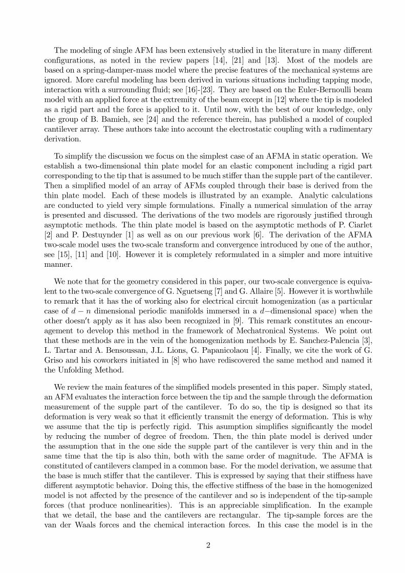
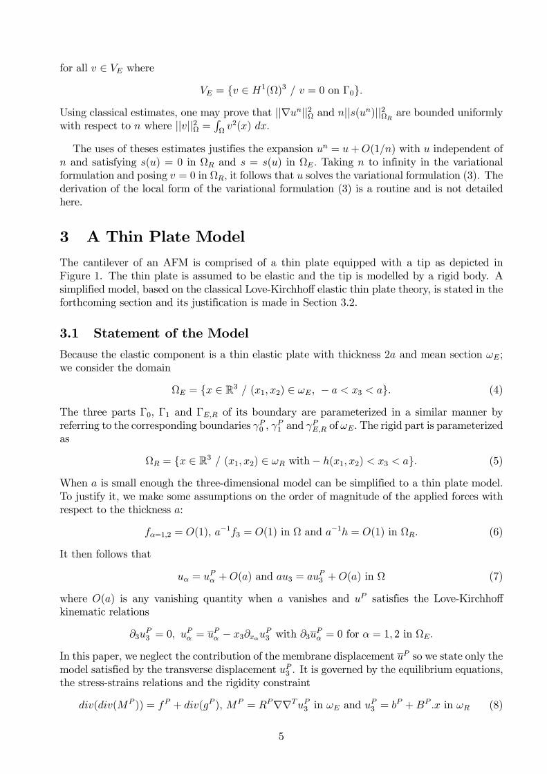
2 Three-Dimensional ModelWe start by considering a mechanical structure located in Ω ⊂ R3 made up of an elastic partand a rigid part located respectively in ΩE and in ΩR as depicted in Figure 1. The model isstated in the next section and subsequently justified in Section 2.2.

2.1 Statement of the Model

The elastic component is clamped along part of its boundary Γ0, is linked to the rigid partthrough the interface ΓE,R and is free of applied forces in the remaining part Γ1. When thesystem is totally elastic (no rigid part), then ΩR and ΓE,R are void and the related equationmust be ignored. The mechanical displacements are denoted by the vector u = (u1, u2, u3)

T

defined over the entire structure.

a

x

x1

x2

x3

Γ0

ΩE

E,RΓ Γ1

RΩ

tip

Figure 1: Three-dimensional plate with the rigid part

The fourth-order elasticity tensor is denoted by R and may vary in space if the materialis not homogeneous. The symmetric matrix of linear strains is s(u) = 1

2(∇u +∇Tu) where ∇

3

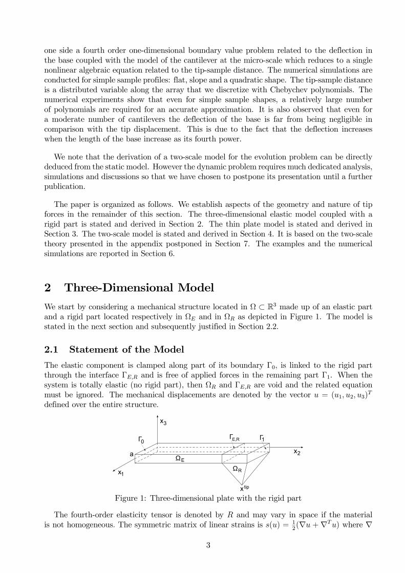
is the gradient operator. The equilibrium equations, the linear stress-strains relation and therigidity constraint are stated as

−div(σ) = f , σ = Rs(u) in ΩE and s(u) = 0 in ΩR (1)

where the product between the fourth-order tensor R and the matrix s(u) gives the 3×3 matrixwith entries

σij =3X

k,l=1

Rijklskl(u).

In the case of isotropic elasticity, the elasticity tensor has the form

Rijkl = λδijδkl + 2µδikδjl

where δ is the Kronecker delta.The boundary conditions are u = 0 on Γ0, σn = 0 on Γ1 (n being the outward normal vector

to the boundary). Moreover, u will be continuous at the interface ΓE,R. Finally, the force andforce momentum transmissions satisfyZ

ΓE,R

σ n ds = ξ,ZΓE,R

(σ n).(x× ek) ds = Ξk for k ∈ 1, 2, 3 (2)

where

ξ =

ZΩR

f(x)dx, Ξk =ZΩR

f(x).(x× ek)dx.

We note that the condition s(u) = 0 can be formulated through imposing a rigid displacementu = b+x×B whose b and B are some three dimensional vectors. The variational formulation,which is necessary for the formulation of Galerkin-like numerical methods, can be formulatedas follows: find u ∈ V such that Z

ΩE

σ :: s(v) dx =

ZΩ

f.v dx (3)

for all v ∈ V for the previous stress-strains relationship where the admissible space of testfunctions is

V = v ∈ H1(Ω)3 / s(v) = 0 in ΩR and v = 0 on Γ0.The Sobolev space H1(Ω) is the set of square integrable functions in Ω,

RΩv2(x) dx <∞, such

that each component of their gradient are also square integrable.

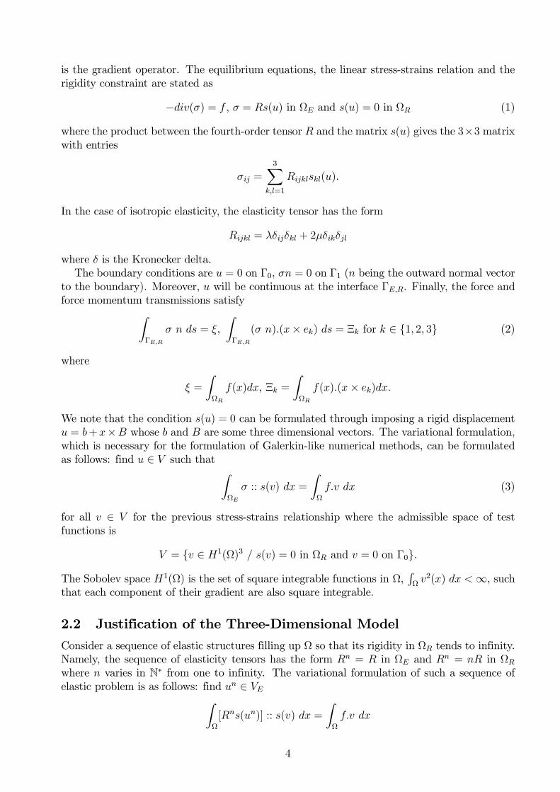
2.2 Justification of the Three-Dimensional Model

Consider a sequence of elastic structures filling up Ω so that its rigidity in ΩR tends to infinity.Namely, the sequence of elasticity tensors has the form Rn = R in ΩE and Rn = nR in ΩRwhere n varies in N∗ from one to infinity. The variational formulation of such a sequence ofelastic problem is as follows: find un ∈ VEZ

Ω

[Rns(un)] :: s(v) dx =

ZΩ

f.v dx

4

for all v ∈ VE whereVE = v ∈ H1(Ω)3 / v = 0 on Γ0.

Using classical estimates, one may prove that ||∇un||2Ω and n||s(un)||2ΩR are bounded uniformlywith respect to n where ||v||2Ω =

RΩv2(x) dx.

The uses of theses estimates justifies the expansion un = u+O(1/n) with u independent ofn and satisfying s(u) = 0 in ΩR and s = s(u) in ΩE. Taking n to infinity in the variationalformulation and posing v = 0 in ΩR, it follows that u solves the variational formulation (3). Thederivation of the local form of the variational formulation (3) is a routine and is not detailedhere.

3 A Thin Plate ModelThe cantilever of an AFM is comprised of a thin plate equipped with a tip as depicted inFigure 1. The thin plate is assumed to be elastic and the tip is modelled by a rigid body. Asimplified model, based on the classical Love-Kirchhoff elastic thin plate theory, is stated in theforthcoming section and its justification is made in Section 3.2.

3.1 Statement of the Model

Because the elastic component is a thin elastic plate with thickness 2a and mean section ωE;we consider the domain

ΩE = x ∈ R3 / (x1, x2) ∈ ωE, − a < x3 < a. (4)

The three parts Γ0, Γ1 and ΓE,R of its boundary are parameterized in a similar manner byreferring to the corresponding boundaries γP0 , γ

P1 and γ

PE,R of ωE. The rigid part is parameterized

as

ΩR = x ∈ R3 / (x1, x2) ∈ ωR with− h(x1, x2) < x3 < a. (5)

When a is small enough the three-dimensional model can be simplified to a thin plate model.To justify it, we make some assumptions on the order of magnitude of the applied forces withrespect to the thickness a:

fα=1,2 = O(1), a−1f3 = O(1) in Ω and a−1h = O(1) in ΩR. (6)

It then follows that

uα = uPα +O(a) and au3 = au

P3 +O(a) in Ω (7)

where O(a) is any vanishing quantity when a vanishes and uP satisfies the Love-Kirchhoffkinematic relations

∂3uP3 = 0, u

Pα = u

Pα − x3∂xαuP3 with ∂3u

Pα = 0 for α = 1, 2 in ΩE.

In this paper, we neglect the contribution of the membrane displacement uP so we state only themodel satisfied by the transverse displacement uP3 . It is governed by the equilibrium equations,the stress-strains relations and the rigidity constraint

div(div(MP )) = fP + div(gP ), MP = RP∇∇TuP3 in ωE and uP3 = bP +BP .x in ωR (8)

5

where

gPα (x1, x2) =

Z a

−afα(x)x3 dx3 and fP (x1, x2) =

Z a

−af3(x) dx3 in ωE. (9)

In the case of isotropic materials, the elasticity can be formulated as

RPαβγρ = a3(

4λµ

3(λ+ 2µ)δαβδγρ +

4µ

3δαγδβρ). (10)

In addition, x = (x1, x2)T , bP is a scalar and BP is a two-dimensional vector.

The boundary conditions are

uP3 = ∇uP3 .n = 0 on γP0 (11)

and nTMPn = 0, ∇(nTMP τ ).τ + div(MP ).n = gP .n on γP1

where n and τ are the unit outward normal and the unit tangent to the boundary of ωE.The transmission condition at the interface γE,R results from the continuity conditions of thedisplacement uP3 and of its gradient ∇uP3 and the continuity of the normal stresses. These canbe expressed as

bP = |γE,R|−1ZγE,R

(uP3 −∇uP3 .x)|ωE ds, BP = |γE,R|−1ZγE,R

(∇uP3 )|ωE ds (12)

−ZγE,R

div(MP ).n ds = ξP andZγE,R

nTMP − (div(MP ).n)x ds = ΞP

where

ξP = −ZγE,R

(gP .n)|ωE ds+ZωR

fP dx, ΞPα = −ZγE,R

(gP .n)|ωExα ds+ZωR

fPxα − gPα dx,

|γE,R| denotes the length of the interface γE,R, gP and fP having been defined in ωE and aredefined in ωR by

gPα (x1, x2) =

Z a

−h(x1,x2)fα(x)x3 dx3 and fP (x1, x2) =

Z a

−h(x1,x2)f3(x) dx3 in ωR.

The variational formulation associated with this model is

uP3 ∈ V P andZωE

MP :: ∇∇Tv dx =ZωP

fPv − gP .∇v dx for all v ∈ V P (13)

taking into account the stress-strains relation. The set of admissible transverse displacementsis

V P = v ∈ H2(ωP ) / ∇∇Tv = 0 in ωR and v = 0 on γP0 and H2(ωP ) being the set of square integrable functions on ωP so that their first order andsecond order derivatives are also square integrable.

Remark 1 For the derivation of the two-scale model, we need an extension of this model forplates with varying thickness, namely, when ΩE and ΩR are replaced by

ΩE = x ∈ R3 / (x1, x2) ∈ ωE and − k(x1, x2) < x3 < k(x1, x2)ΩR = x ∈ R3 / (x1, x2) ∈ ωR with− h(x1, x2) < x3 < k(x1, x2)

where k is a positive function so that a−1k = O(1). In such a case, the model remains the sameexcepted that a is replaced by k in the expressions of the two-dimensional forces (9) and of thetwo-dimensional rigidities (10).

6

3.2 Justification of the Thin Plate Model

The justification of the thin plate model is based on the asymptotic method of P.G. Ciarlet [2]and of P. Destuynder [1]. In these works, the thin plate model is derived for isotropic elasticbodies by calculating the asymptotic behavior of the elasticity system and of its solution whenthe parameter a vanishes. In this work we use the same method but our derivation is basedon the paper E. Canon and M. Lenczner [6] where material anisotropy was encompassed. Theonly difference between the new model and that in [6] comes from the presence of the rigidbody which does not significantly affect the proofs. Hence we report only the main steps in thecalculations.

Since the asymptotic method consist of finding the limit when a vanishes, it is mandatory tointroduce a scaled domain independent of a and to formulate the problem on it. To do so, oneintroduces the change of variable F a defined on Ω by F a(x) = (x1, x2, 1ax3) in Ω. The imageF a(Ω) is denoted by eΩ and there the coordinates are ex = F a(x). The whole model is nowexpressed on the dilated domain. All variables or fields related to eΩ are covered by a tilde. Therigidity, the mechanical displacement and the forces are scaled in different manners

eR(ex) = R(x), eu(ex) = (u1, u2, au3)(x), ef(ex) = (f1, f2, 1af3)(x) for x ∈ Ω.

From the assumption made on f , it is clear that || ef ||eΩ is bounded. We also apply a scaling tothe test functions

ev(ex) = (v1, v2, av3)(x).For a given displacement field v, define the 3 × 3 matrice K(ev) such that Kαβ(ev) = sαβ(ev),Kα3(ev) = K3α(ev) = a−1s3α(ev) andK33(ev) = a−2s33(ev). Applying the variable change ex = F a(x)in (3) yields the following variational formulation: find eu ∈ eV such that

a

ZeΩE eσ :: K(ev) dex = a

ZeΩ ef(ex).ev(ex) dex (14)

for all ev ∈ eV where eσ = eRK(eu) andeV = ev ∈ H1(eΩ)3 / K(ev) = 0 in eΩR and ev = 0 on eΓ0.

By equating ev = eu, one may prove that ||eu||eΩ and ||K(eu)||eΩ are O(1) with respect to a. Thuswe are led to formulate

eu = euP +O(a), K(eu) = KP +O(a)

where euP and KP are independent of a. It follows that

KPαβ = sαβ(euP ) for α, β = 1, 2 and that si3(euP ) = 0 for i = 1, 2, 3.

This is equivalent to saying that euP fulfils the Love-Kirchhoff kinematics∂ex3euP3 = 0 and euPα = euPα − ex3∂xαeuP3 with ∂ex3euPα = 0.

When neglecting the membrane displacement euα, it appears that euP3 solves the variationalformulation, which is independent of the parameter a,

7

euP3 ∈ V P , ZωE

fMP :: ∇∇Tev3 dex = ZeΩ ef3 ev3 − ex3 efα∂exαev3 dex for all ev3 ∈ V P .Here fMP = eRP∇∇TeuP3 and eRP is defined under the name Q22 in E. Canon and M. Lenczner[6] and is equal to

eRPαβγρ = 4λµ

3(λ+ 2µ)δαβδγδ +

4µ

3δαγδβρ

in the case of an isotropic material. Applying the inverse variable change, uP3 solves the varia-tional formulation: find uP3 ∈ V P such thatZ

ωE

MP :: ∇∇Tv3 dx =ZΩ

(f3 v3 − x3fα∂xαv3) dx

for all v3 ∈ V P with MP = RP∇∇TuP3 and RP = a3 eRP . This leads directly to the variationalformulation (13). Since ∇∇Tv3 = 0 in ΩR it may be written v3 = d+D.x with D = (D1,D2)T

thus the right hand side may be reformulated asZωE

(fP v3 − gP .∇v3) dx+ ξPdP + ΞP .DP .

Application of twice Green formula and using the fact that v3 = d + D.x on γE,R, it followsthat Z

ωE

div(div(MP )v3 dx+

Zγ1

(nTMP∇v3 − div(MP ).n v3) ds

−(ZγE,R

div(MP ).n ds) dP + (

ZγE,R

(nTMP − div(MP ).n x) ds).DP

=

ZωE

(fP3 + div(gP ))v3 dx−

Zγ1

gP .n v3 ds+ ξPdP + ΞP .DP

from which we deduce all the model equations excepted the continuity condition of uP3 and∇uP3 that comes by integrating the expressions uP3 = bP +BP .x and ∇uP3 = BP on γE,R.

4 Model for an AFM ArrayConsider a mechanical structure made of a periodic distribution of microcantilevers as shownon Figure 2. In Section 4.1 a simplified model is stated when its derivation is done in Section4.2.

4.1 Statement of the Model

The whole domain occupied by the cantilever array is still denoted by ωP and is assumed tobe embedded in the macroscopic domain ω = (0, L1)× (0, L2). It is constituted of n×n squarecells Y ε

i of size ε× ε and fills up ω which constrains the parameter ε to be equal to 1/n.

8

0

By

FyRy

1/2

-1/2 1/2

-1/2

1y

2y

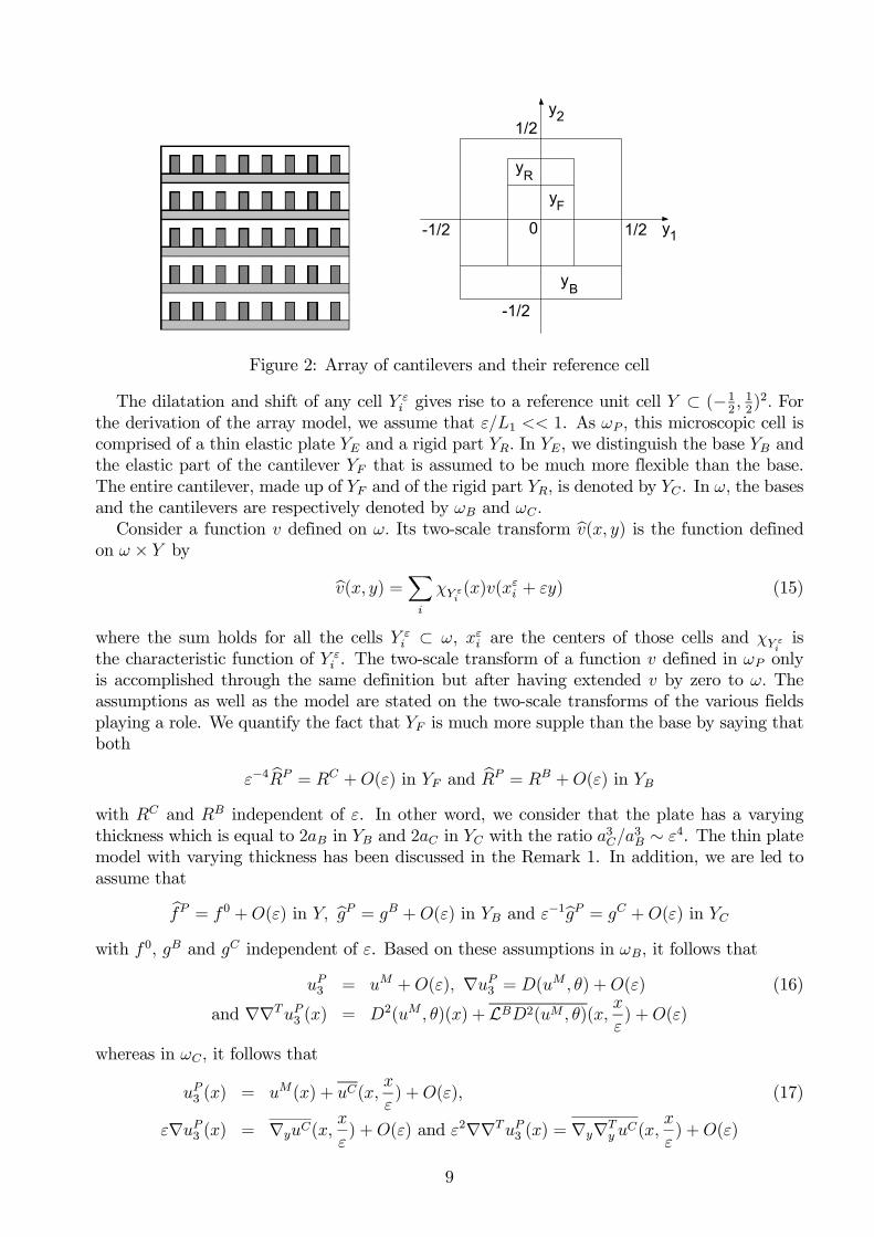
Figure 2: Array of cantilevers and their reference cell

The dilatation and shift of any cell Y εi gives rise to a reference unit cell Y ⊂ (−12 , 12)2. For

the derivation of the array model, we assume that ε/L1 << 1. As ωP , this microscopic cell iscomprised of a thin elastic plate YE and a rigid part YR. In YE, we distinguish the base YB andthe elastic part of the cantilever YF that is assumed to be much more flexible than the base.The entire cantilever, made up of YF and of the rigid part YR, is denoted by YC . In ω, the basesand the cantilevers are respectively denoted by ωB and ωC .Consider a function v defined on ω. Its two-scale transform bv(x, y) is the function defined

on ω × Y bybv(x, y) =X

i

χY εi(x)v(xεi + εy) (15)

where the sum holds for all the cells Y εi ⊂ ω, xεi are the centers of those cells and χY ε

iis

the characteristic function of Y εi . The two-scale transform of a function v defined in ωP only

is accomplished through the same definition but after having extended v by zero to ω. Theassumptions as well as the model are stated on the two-scale transforms of the various fieldsplaying a role. We quantify the fact that YF is much more supple than the base by saying thatboth

ε−4 bRP = RC +O(ε) in YF and bRP = RB +O(ε) in YBwith RC and RB independent of ε. In other word, we consider that the plate has a varyingthickness which is equal to 2aB in YB and 2aC in YC with the ratio a3C/a

3B ∼ ε4. The thin plate

model with varying thickness has been discussed in the Remark 1. In addition, we are led toassume thatbfP = f 0 +O(ε) in Y, bgP = gB +O(ε) in YB and ε−1bgP = gC +O(ε) in YCwith f 0, gB and gC independent of ε. Based on these assumptions in ωB, it follows that

uP3 = uM +O(ε), ∇uP3 = D(uM , θ) +O(ε) (16)

and ∇∇TuP3 (x) = D2(uM , θ)(x) + LBD2(uM , θ)(x,x

ε) +O(ε)

whereas in ωC , it follows that

uP3 (x) = uM(x) + uC(x,x

ε) +O(ε), (17)

ε∇uP3 (x) = ∇yuC(x, xε) +O(ε) and ε2∇∇TuP3 (x) = ∇y∇Ty uC(x,

x

ε) +O(ε)

9

where ∇y is the gradient with respect to y,

D(uM , θ) =

µ∂x1u

M

θ

¶and D2(uM , θ) =

µ∂2x1x1u

M ∂x1θ∂x1θ 0

¶and v is defined in (54). The construction of (uM , θ), of the fourth order tensor LB and of uCis done as follows. First, one builds LB so that

(∇y∇TywB)αβ =2X

γ,ρ=1

LBαβγρµ

ν µµ 0

¶γρ

(18)

where wB is solution of the microscopic problem PB posed in the base YB. Once this is done,the calculation of (uM , θ) is made possible by solving the problem macro PM related to themacroscopic domain ω and the base YB. Finally, uM being known, uC may be computed due tothe microscopic problem PC posed in YC . We note that in the case of atomic forces dependingon uC , the macroscopic problem PM and the microscopic problem PC in the cantilever cannotbe solved sequentially since they are fully coupled through the expression of the atomic forceswhen its action on the tip has a non negligible effect on the base0s solution (uM , θ).

Problem PM : The set of edges of the macroscopic domain ω where x1 = 0 or 1 splits inγM0 and γM1 corresponding, respectively, to the area where the base is clamped and where it isfree. The statement of the macroscopic or homogenized problem PM includes the equilibriumequations

∂2x1x1MM1 = fM1 and ∂x1M

M2 = fM2 in ω (19)

and the stress-strains relation

MM1 = RM11∂

2x1x1

uM +RM12∂x1θ, MM2 = RM21∂

2x1x1

uM +RM22∂x1θ in ω (20)

along with the boundary conditions

uM = ∂x1uM = θ = 0 on γM0 (21)

and MM1 = MM

2 = 0, ∂x1MM1 = gM on γM1 .

The new parameters are

gM =

ZYB

gB1 dy, fM1 =

ZY

f0 dy +

ZYB

∂x1gB1 dy, f

M2 =

ZYB

gB2 dy

RM =

à eRM1111 2 eRM12112 eRM1211 4 eRM1212

!

where the fourth order tensor eRM is defined by

eRMαβγρ = ZYB

RBαβγρ +RBαβξζLBξζγρ dy,

LB is defined by (18) and wB is solution of the problem PB.The variational formulation is

(uM , θ) ∈ V M ,Zω

MM .(∂2x1x1v, ∂x1η)T dx =

Zω

fM1 v − gM .D(v, η) dx for all (v, η) ∈ V M (22)

10

where

V M = (v, η) ∈ L2(ω)2 / ∂2x1x1v and ∂x1θ ∈ L2(ω), v = ∂x1v = θ = 0 on γM0 ,L2(ω) being the set of square integrable functions on ω.

Problem PB : The boundary of YB is made up of the interface γB,F between YB and YF ,the area γper corresponding to the junction between neighboring cells and the remaining partγB1. The microscopic equations stated in the base YB are

divy(divy(MB)) = −divy(divy(FB)) with MB = RB∇y∇TywB and FB = RB

µν αα 0

¶. (23)

The boundary conditions are

∇y(nTyMBτ y).τ y + divy(MB).ny = −∇y(nTy FBτ y).τ y − divy(FB).ny

and nTyMBny = −nTy FBny on γB1 ∪ γB,F

and

wB, nTyMBny, ∇wB.n, ∇y(nTyMBτ y).τ y + divy(M

B).ny are Y − periodic on γper.

Finally, wB and ∇ywB are set equal to zero in an arbitrary point y0 of YB so that to garanteethe uniqueness. The variational formulation is

uB ∈ V B,ZYB

MB :: ∇y∇Ty v dy = −ZYB

FB∇y∇Ty v dx for all v ∈ V B (24)

where

V B = v ∈ H2(YB) / v, ∇yv are Y − periodic on γper.We note that the solution of this variational formulation is unique up to a function v such that∇y∇Ty v = 0 and v, ∇yv are Y−periodic on γper, in short up to a function v(y) = a0 + a1y2.

Problem PC . The boundary of the elastic part YF of the cantilever is the union of theinterface γB,F between the base and the cantilever, the interface γB,R between the elastic part

and the rigid part and the remaining γF1. The data cfP and gC being given, the problem PCused for the calculation of uC is made up of the equilibrium equations, the stress-strains relationand the rigidity constraint

divy(divy(MC)) = f0 + divyg

C and MC = RC∇y∇Ty uC in YF , (25)

uC = bC +BC .y in YR,

the boundary conditions

uC = ∇yuC .ny = 0 on γB,F ,

nTyMCny = 0, ∇y(nTyMCτ y).τ y + divy(M

C).ny = 0 on γF1,

the continuity of uC and ∇yuC through the interface γF,R and the normal stresses transmission

bC = |γF,R|−1ZγF,R

(uC −∇uC .x)|YF ds, BC = |γF,R|−1ZγF,R

(∇uC)|YF ds

−ZγF,R

divy(MC).ny ds = ξC ,

ZγF,R

nTyMC − (divy(MC).ny)y ds = ΞC

11

where

ξC =

ZYR

f 0 dy −ZγF,R

(gC .ny)|YF ds and ΞC =

ZγF,R

−(gC .ny)|YF y ds+ZYR

f 0 y − gC dy.(26)

The corresponding variational formulation is

uC ∈ V C ,ZYF

MC :: ∇y∇Ty v dy =ZYC

f0v − gC .∇yv dy for all v ∈ V C (27)

where

V C = v ∈ H2(YC) / v = ∇yv.ny = 0 on γB,F , ∇y∇Ty v = 0 in YR.

4.2 Derivation of the Two-scale Model

The proof follows three steps. First a specific estimate of the growth of the mechanical dis-placement is derived with respect to the small parameter ε. In a second step we use the Taylorexpansion of the two scale transform of uP and identify the global system which is verified bythe coefficients of the Taylor expansion. It is from this global system that the wanted model isextracted.The mathematical formulation of the assumptions on the rigidity and on the external forces

is in the one side an uniform ellipticity condition: there exists a constant K such that for allε > 0 and all 2× 2 symmetric matrix ξ,

[RBξ] :: ξ and [RCξ] :: ξ ≥ K|ξ|2

and in the other side there exists another constant C such that for all ε > 0,

|| bfP ||ωP×Y + ||bgP ||ωP×YB + ||gC||ωP×YC ≤ C.In the proof, for the sake of simplicity, we remove the uperscript of uP3 , f

P and gP .

(i) Let us prove the estimates

||u||ωP , ||∇u||ωB , ||ε∇u||ωC , ||∇∇Tu||ωB , ||ε2∇∇Tu||ωC ≤ C (28)

uniformly with respect to ε. One starts from the variational formulation (13) where one equalesv = u Z

ωB

[RP∇∇Tu] :: ∇∇Tu dx+ZωF

ε−4[RP (ε2∇∇Tu)] :: (ε2∇∇Tu) dx

=

ZωP

f.u− χωBg.∇u− χωC

ε−1g.(ε∇u) dx,

one applies the uniform ellipticity condition and use the fact that ∇∇Tu = 0 in ωR,

X = K(||∇∇Tu||2ωB + ||ε2∇∇Tu||2ωC ) ≤ ||f ||ωP ||u||ωP + ||(χωB+ ε−1χωC

)g||ωP ||(χωB+ εχωC

)∇u||ωP ,

and then the estimates on the external forces

X ≤ C1(||u||ωP + ||(χωB+ εχωC

)∇u||ωP ).

12

Thanks to the Poincaré like estimate (66),

X ≤ C2||(χωB+ ε2χωC

)∇∇Tu||ωP .The third estimate in (28) follows and the two others are a direct consequence of it and of (66).

(ii) Let us establish that (uM , θ, uB, uC) is solution of the two-scale variational formulation:

(uM , θ, uB, uC) ∈ V,Zω×YB

M :: [D2(vM , η) +∇y∇Ty vB] dydx+Zω×YF

MC :: ∇y∇Ty vC dydx =(30)Z

ω×YPf 0.vM dydx−

Zω×YB

gB.D(vM , η) dydx−Zω×YC

gC .∇yvC dydx+O(ε)

for all (vM , η, vB, vC) ∈ V withM = RB(D2(uM , θ) +∇y∇Ty uB), MC = RC∇y∇Ty uC

and

V = VM × L2(ω;V B)× L2(ω;V C)where

VM = (vM , η) ∈ H2(ω)×H1(ω) / vM = ∇vM .n = θ = 0 on γM0 .We assume that u can be expanded as bu = u0+ εu1+ ε2u2+ ε2O(ε) which is partially justifiedby (28). We make use of the results stated in the appendix for ω1 = ωP and thus d = 2. Thedomain ωP is clearly not connected in the direction x2 parallel to the cantilevers and connectedin the direction x1 parallel to the base.Let us make the link between the general notation used in the appendix and the specific

notations of the two-scale model presented in this paper. We pose

uM = u0|ω×YB , θ = ∂y2u1 and uB = u2 in ω × YB,

uC = u0 − uM in ω × YC .Thus (uM , θ, uB, uC) ∈ V and

(bu, c∇u, \∇∇Tu) = (uM ,D(uM , θ), D2(uM , θ) +∇y∇Ty uB) +O(ε) in ω × YB, (31)

and (bu, εc∇u, ε2\∇∇Tu) = (uM + uC ,∇yuC ,∇y∇Ty uC) +O(ε) in ω × YCwhere the approximations are in the weak sense as defined in appendix. Now consider the testfunctions (vM , η, vB, vC) ∈ V and v1 such that ∂y2v1 = η. Let us pose

v = vM + εv1 + ε2vB in ω × YB and v = vM + vC in ω × YC .We restrict to regular functions v1 and v2 such that v1 satisfies the boundary conditions so thatthey belong to V P . Then according to the definition (54), it appears that v(x, x

ε) ∈ V P and it

may be chosen as a test function in the variational formulation (13) that we rewrite:

u ∈ V P ,

ZωB

MP :: ∇∇Tv dx+ZωF

MP1 :: (ε2∇∇Tv) dx (32)

=

Zω

f.v dx−ZωB

g.∇v dx−ZωC

(ε−1g).(ε∇v) dx

13

with

MP1 = (ε−4RP )(ε2∇∇Tu).Let us focus our attention to the first integral. We remark that

∇∇Tv = (D2(vM , η) +∇y∇Ty vB)(x,x

ε) +O(ε) in ωB

From (56) it is also approximated by T ∗(EYB(D2(vM , η) +∇y∇Ty vB))(x) +O(ε) so

X =

ZωB

MP :: ∇∇Tv dx =Zω

EωBMP :: T ∗(EYB(D

2(vM , η) +∇y∇Ty vB)) dx+O(ε)

because ||MP ||ωB is bounded. Here EωB and EYB denote the operators that extend by 0 afunction defined on ωB or YB to a function defined in ω or Y. Let us rewrite it by transposingT ∗:

X =

Zω×Y

\EωBMP :: EYB(D

2(vM , η) +∇y∇Ty vB) dx+O(ε).

Using the identity T (EωBMP ) = EYBR

B\∇∇Tu and the approximation of \∇∇Tu yields

X =

Zω×YB

[RB(D2(uM , θ) +∇y∇Ty uB)] :: (D2(vM , η) +∇y∇Ty vB) dx+O(ε)

which is the first term of (30). The same procedure applied to each terms of (32), providedthat

∇v = D(vM∗, η)(x,x

ε) +O(ε) in ωB

and ε∇v = ∇yvC(x, xε) +O(ε), ε2∇∇Tv = ∇y∇Ty vC(x,

x

ε) +O(ε) in ωC ,

leads to the complete formulation (30).(iii) From the two-scale variational formulation, we now derive successively the three prob-

lems PB, PC and PM .For the derivation of PB one starts by choosing η = vM = vC = 0 and remark that

MM = RBD2(uM , θ) +MB

then Zω×YB

MB :: ∇y∇Ty vB dydx =Zω×YB

−[RBD2(uM , θ)] :: ∇y∇Ty vB dydx.

Making the choice vB(x, y) = ϕ(x)evB(y) with any regular ϕ vanishing on the boundary of ωallows us to eliminate the integrals over ω and yields the variational formulation (23) where wehave removed the O(ε) term.For the derivation of PC one poses η = vM = vB = 0 which leads toZ

ω×YFMC :: ∇y∇Ty vC dydx =

Zω×YC

bf.vM − gC .∇yvM dydx.

Based on the same argument, the integrals over ω may be removed and (25) follows.

14

Finally one derives PM by posing vB = vC = 0 and using the fact that

∇y∇Ty uB = LBD2(uM , θ). (33)

It follows that

Zω

MM :: D2(vM , η) dydx =

Zω×YP

bf.vM dydx−Zω×YB

bg.D(vM , η) dydxand the variational formulation (22) follows. The final approximation of uP and of their deriva-tives comes from the application of T ∗ to (31) plus the linear relation (33) and finally thegeneral approximation T ∗v(x) = v(x,

x

ε).

5 Tip ForcesTo characterize the behavior of the cantilever, it is necessary to quantify the attractive forcesF vdW of van der Waals type and repulsive forces F rep between the tip and sample. We considerfirst the development of relations for F vdW .As detailed in [28, 21], attractive forces result primarily from van der Waals forces that are

due to a combination of electrostatic and dispersional effects present between all atoms andmolecules. Either classical or quantum principles can be used to derive the van der Waalspotential

W vdW (ζ) = − C

||ζ||6 where ζ = x0 − x (34)

for two atoms or molecules located respectively at the positions x and x0. Here ||ζ|| = (ζ21 +ζ22 + ζ23)

1/2 and C = α20ν(4πε0)2

is a constant which depends on the electronic polarizability α0 ofconstituent atoms, Planck0s constant , the electron orbital frequency ν, and the permittivityε0 of vacuum.

(a)

(b)

ζ

Ω ΩρΩ

ρΩ

Ω

ρΩ

ρΩΩ

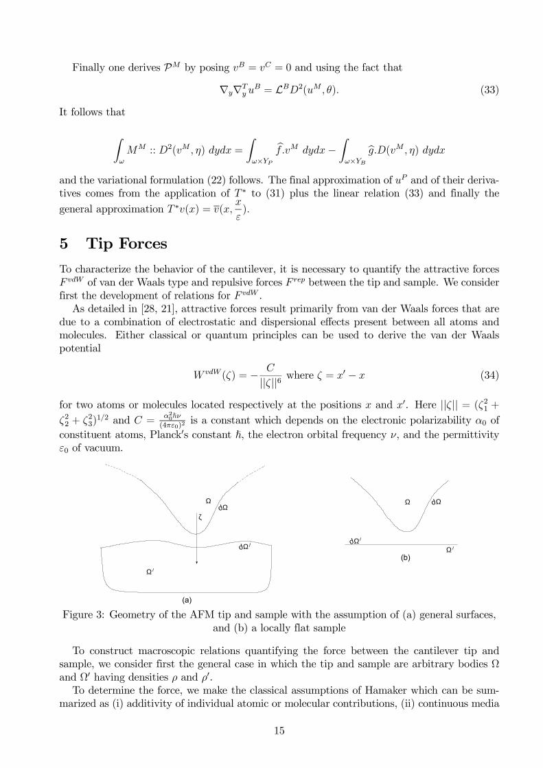
Figure 3: Geometry of the AFM tip and sample with the assumption of (a) general surfaces,and (b) a locally flat sample

To construct macroscopic relations quantifying the force between the cantilever tip andsample, we consider first the general case in which the tip and sample are arbitrary bodies Ωand Ω0 having densities ρ and ρ0.To determine the force, we make the classical assumptions of Hamaker which can be sum-

marized as (i) additivity of individual atomic or molecular contributions, (ii) continuous media

15

so that summation can be replaced by integration, and (iii) constant material properties. Forthese assumptions, the force exerted by the particule located in x0 on this in x is given by

F vdW = ρρ0ZΩ

ZΩ0f(x0 − x) dxdx0 (35)

where f = −∇W .The determination of F for arbitrary geometries and potentialW necessitates approximation

of integrals over six dimensions which is typically prohibitive. To simplify the formulation, wefollow the approach of [26, 27] and reformulate the relation in terms of surface integrals. Weconsider the vector field

G =−Cζ3||ζ||6 . (36)

It follows that

divG = −W (37)

and hence the divergence theorem can be invoked to formulate the macroscopic force as

F vdW = ρρ0Z∂Ω

Z∂Ω0(G.n0)n ds0ds (38)

where n and n0 respectively denote normals to the tip and sample. For the vector field relation(36), the force is

F vdW = − A

3π2

Z∂Ω

Z∂Ω0

ζ .n0

||ζ||6n ds0ds (39)

where the Hamaker constant is

A = π2Cρρ0. (40)

The flat sample case: For various applications, it is reasonable to approximate the sampleby a locally flat surface (n0 constant) while retaining the general representation for the cantilevertip, see Figure 3 (b). For example, this assumption is reasonable when identifying the tip shapeusing a known sample with minimal curvature or for regimes in which the separation distanceis large compared with perturbations in the sample. From the approximationZ

∂Ω0

ζ.n0

||ζ||6n ds ≈ZR2

ζ.n0

||ζ||6 dx01dx

02 =

ZR2

ζ.n0

||ζ||6 dζ1dζ2 =π

2(ζ .n0)3.

the attractive force is

F vdW =A

6π

Z∂Ω

n

(ζ.n0)3ds. (41)

The simplified force relation (41) facilitates implementation when identifying the tip shape oroperating in regimes in which the separation distance is sufficiently large so that modulationsin the sample surface are negligible.

16

R

d

θ

γ

x3

Figure 4: Geometry of the AFM tip

Flat sample and parameterized tip: Finally, we consider the case in which the samplesurface is assumed locally flat and a simple geometric parameterization is assumed for thecantilever tip. Specifically, we follow the approach of Argento and French [26] and assume thatthe cantilever can be parameterized as having a spherical tip of radiusR, and a conical section asdepicted in Figure 3 with a distance d from the sample. This geometry is motivated by scanningelectron microscopy (SEM) images of various AFM tips and provides sufficient flexibility for anumber of applications while limiting to commonly employed models for spherical probes.This assumption allows cylindrical symmetry to be invoked to yield analytic force relations,

and relaxation of this assumption would necessitate the approximation of nonsymmetric con-tributions which yield higher-order force effects.As detailed in [26], the attractive force due to van der Waals interactions can in this case be

expressed as

F vdW (d) =AR2[1− sin γ][R sin γ − d sin γ −R− d]

6d2[R+ d−R sin γ]2 − A tan γ[d sin γ +R sin γ +R cos(2γ)]6 cos γ[d+R−R sin γ]2

(42)

where A is the Hamaker constant specified in (40) and γ is the cone angle shown in Figure 3.The repulsive forces are due to the overlap of electron clouds. These are quantum mechan-

ical in nature and very short range compared with the attractive forces. Phenomenologicalarguments yield microscopic potential relations of the form

W rep(ζ) =B

||ζ||12 (43)

where B is a constant which depends on electronic and material properties of the sample andtip. Arguments analogous to those for the attractive forces yield short-range force relationsanalogous to (39), (??), or (42).

6 ExamplesAn example illustrating the application of the thin plate model for an AFM is presented inSection 6.1. In Section 6.2, the two-scale model is applied to an AFM array. Finally in Section6.3, results for a simulation of the AFM array are reported and discussed.

17

6.1 A Single AFM

The two-dimensional domain ωP is a rectangle ωP = (0, `0C)×(0, LC) with `0C << LC . The plateis made up of an homogeneous isotropic material, is clamped on the side x1 = 0 and is left freeotherwhere. The elastic part is ωE = (0, `0C)× (0, LE) and the rigid part is its complementaryset ωR = (0, `0C)× (LE, LC). The coordinates of the tip are xtip = (xtip1 , xtip2 , xtip3 ). The shape ofthe sample to be analyzed is parameterized by a function φ(x1, x2). The force applied on thetip is modelled as a concentrated force

f1 = f2 = 0 and f3(x) = F (d)δxtip(x)

where d = utip− φtipwith φtip = φ(xtip1 , xtip2 ) and u

tip = u(xtip). Let us denote by xG the gravitycenter of ΩR and assume that xtip − xG is parallel to the direction of x3. If the dependency ofuP3 with respect to x1 is neglected, then the distance d between the tip and the sample is theunique solution of the nonlinear algebraic equation

kP (xtip2 )(d+ φtip)− F (d) = 0 (44)

and when d is known uP3 is computed by

uP3 (x2) = F (d)/kP (x2) for x2 ∈ [0, LC ]

where

kP (x2) =6mP

x22(3HP |ωR|/|ΩR|− x2) in [0, LE]

=6|ΩR|mP

LE(−3LEHP |ωR|+ 2L2E|ΩR|+ 6x2HP |ωR|− 3x2LE|ΩR|) in (LE, LC ],

and

mP =8µa3(λ+ µ)`0C3(λ+ 2µ)

, (45)

hP = |ωR|−1|ΩR|, HP = |ωR|−1ZωR

(a+ h(x))x2 dx.

The proof is straightforward and we mention only the main steps. From Section 7.4,

fP (x) =a+ h(x)

|ΩR| F (d) in ωR, fP = 0 in ωE, g

P = 0 in ωP ,

thus

ξP =

ZωR

a+ h(x)

|ΩR| dx F = F and ΞP2 =HP |ωR||ΩR| F.

The displacement uP3 is solution of the boundary value problem

d4uP3dx42

(x2) = 0 for x2 ∈ (0, LE), uP3 (0) =duP3dx2

(0) = 0

(46)

−mP d3uP3dx32

(LE) = ξP and mP (d2uP3dx22

− d3uP3dx32

x2)(LE) = ΞP2

18

where mP = `0CRP2222. In the rigid part

uP3 (x2) = bP +BP2 x2

with

bP = uP3 (LE)−duP3dx2

(LE)LE and BP2 =duP3dx2

(LE).

In particular,

utip = bP +BP2 xtip2 .

The equations (46) yield uP3 (x2) = a0 + a1x2 + a2x22 + a3x

32 in the elastic part with

a0 = a1 = 0, 2mPa2 = ΞP2 and − 6mPa3 = ξP (47)

from which the equation uP3 (x2) = F (d)/kP (x2) follows. The equation of d follows by taking

x2 = xtip2 and using the relation uP3 (x

tip2 ) = d+ φtip.

6.2 An AFM Array

The whole system is still comprised of a homogeneous isotropic material. The subdomains YBand YC are two rectangles described respectively in the coordinates (OB, yB1 , y

B2 ) and (OC , y

C1 , y

C2 )

by

YB = (0, 1)× (0, `B) and YC = (0, `0C)× (0, LC)

where OC = (− `0C2, `B − 1

2), OB = (−12 ,−1

2), yB = y − OB and yC = y − OC , see Figure 5 for

the description of the cell and Figure 4 for the changes of coordinates. The flexible part YF ofYC is (0, `0C)× (0, LF ) in (OC , yC).

-1/2

1/2-1/2

1/2

0

lB

lcy2

y1

Lc

LF

tipy

Figure 5: Reference cell

We assume that γM1 = ∅ so γM0 = 0, 1 × (0, 1). The tip coordinates are denoted by ytip in(O, y1, y2), by yCtip in (OC , yC1 , y

C2 ) and by x

tipi = (xtipi1 , x

tipi2 , x

tipi3 ) in Ω.

19

C

0

yy

y2

2B

2

0C

0B

y1

y1C

y1B

y c tip

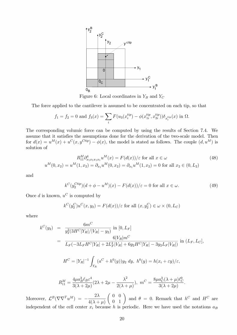
Figure 6: Local coordinates in YB and YC

The force applied to the cantilever is assumed to be concentrated on each tip, so that

f1 = f2 = 0 and f3(x) =Xi

F (u3(xtipi )− φ(xtip1i , x

tip2i ))δxtipi

(x) in Ω.

The corresponding volumic force can be computed by using the results of Section 7.4. Weassume that it satisfies the assumptions done for the derivation of the two-scale model. Thenfor d(x) = uM(x) + uC(x, yCtip) − φ(x), the model is stated as follows. The couple (d, uM) issolution of

RM11∂4x1x1x1x1

uM(x) = F (d(x))/ε for all x ∈ ω (48)

uM(0, x2) = uM(1, x2) = ∂x1u

M(0, x2) = ∂x1uM(1, x2) = 0 for all x2 ∈ (0, L2)

and

kC(yCtip2 )(d+ φ− uM)(x)− F (d(x))/ε = 0 for all x ∈ ω. (49)

Once d is known, uC is computed by

kC(yC2 )uC(x, y2) = F (d(x))/ε for all (x, yC2 ) ∈ ω × (0, LC)

where

kC(y2) =6mC

y22(3HC|YR|/|VR|− y2) in [0, LF ]

=6|VR|mC

LF (−3LFHC|YR|+ 2L2F |VR|+ 6y2HC|YR|− 3y2LF |VR|) in (LF , LC ],

HC = |YR|−1ZYR

(aC + h0(y))y2 dy, h0(y) = h(xi + εy)/ε,

RM11 =4µa3B`Bε

4

3(λ+ 2µ)(2λ+ 2µ− λ2

2(λ+ µ)), mC =

8µa3C(λ+ µ)`0C

3(λ+ 2µ).

Moreover, LB(∇∇TuM) = − 2λ

4(λ+ µ)

µ0 00 1

¶and θ = 0. Remark that hC and HC are

independent of the cell center xi because h is periodic. Here we have used the notations aB

20

and aC for the thickness of the base and of the cantilever divided by ε and VR ⊂ R3 thethree-dimensional dilatation of any of the tips in ΩR.Let us sketch the derivation. From Section 7.4, the surface force in the thin plate model is

fP (x) =Xi

aC + h0((x− xi)/ε)|VR| F (uP (xtipi )− φ(xtipi ))χYi(x)

where xtipi = (xtipi1 , xtipi2 ) and u

P stands for the approximation of u3. Its two-scale transform is

bfP (x, y) = aC + h0(y)

|VR| F (buP (x, ytip)− bφ(x, ytip))/ε2then

f 0(x, y) =aC + h

0(y)

|VR| F (uM(x) + uC(x, ytip)− φ(x))/ε2.

From that expression, one may derive the solutions of the three problems PB, PM and PC .Problem PB : The solution wB of PB is

wB(yB) = − λν

4(λ+ µ)(yB1 )

2.

This is verified by showing that such wB satisfies the variational formulation. Thus

MB =8µK

3(λ+ 2µ)

µλ 00 2(λ+ 2µ)

¶with K = − λν

4(λ+ µ)

and ZYB

MB∇y∇Ty v dy =16µ(λ+ µ)K

3(λ+ 2µ)

ZYB

∂2y1y1v dy

becauseRYB

∂2y2y2v dy = 0 due to the periodicity of ∂y1v on γper. By another way,

FB =4µ

3(

ν

λ+ 2µ

µ2(λ+ µ) 0

0 λ

¶+

µ0 αα 0

¶)

then ZYB

FB∇y∇Ty v dy =4µλν

3(λ+ 2µ)

ZYB

∂2y2y2v dy

becauseRYB

∂2y1y1v dy =RYB

∂2y1y2v dy = 0 due to the periodicity of v and ∂y1v. Finally thevariational formulation Z

YB

MB∇y∇Ty v dy = −ZYB

FB∇y∇Ty v dy

is fulfilled.

Problem PM : It is straightforward to verify that

LBξζγδ = −2λ

4(λ+ µ)δξ2δζ2δγ1δρ1

eRMαβγρ = 4µ`Ba3Bε

3

3(

λ

λ + 2µδαβδγρ + δαγδβρ − λ

2(λ+ µ)(

λ

λ+ 2µδαβδγ1δ1ρ + δα2δ2βδγ1δ1ρ)).

21

It then follows that

RM =

eRM1111 0

016`Bµ

3

with eRM1111 = 4`Bµa3Bε

3

3(λ+ 2µ)(2λ+ 2µ− λ2

2(λ+ µ)).

The macroscopic forces are fM1 (x) = F (d(x))/ε2 and fM2 = 0. Then multiplying the equation

of uM by ε and introducing RM11 = ε eRM1111, one find that uM is solution of the boundary valueproblem (48) and θ is solution of

∂2x1x1θ(x) = 0 for x ∈ ω, θ(0, x2) = θ(1, x2) = 0 for all x1 ∈ (0, 1)thus θ = 0.

Problem PC : The calculations are exactly the same as those for the simple plate modelin Section 6.1 excepted that x, LE, uP3 , ξ

P , ΞP2 , bP , BP2 , ΩR, ωR and H

P are replaced by yC ,LF , u

C , ξC, ΞC2 , bC, BC2 , VR, YR and H

C . Neglecting the variations of uC with respect to y1 itcomes that uC depends of x and y2 only and is solution of the boundary value problem

∂4uC

∂y42= 0 for yC2 ∈ (0, LF ), uC =

∂uC

∂y2= 0 for yC2 = 0 (50)

−`CRP2222ε−4∂3uC

∂y32= ξC and `CRP2222ε

−4(∂2uC

∂y22− ∂3uC

∂y32yC2 ) = ΞC2 for y

C2 = LF

and

ξC(x) = F (d(x))/ε2,

ΞC2 (x) = |VR|−1ZY R(aC + h0(y))y2 dy F (d(x))/ε

2 =|YR|HC

|VR| F (d(x))/ε2.

By introducing mC = `CRP2222ε

−3 The expression of uC follows. Finally by using the relationuC(., y2) = d− uM + φ for yC2 = y

Ctip2 the equation (49) follows.

6.3 Numerical Simulation of the AFM Array

For numerical computation the algebraic equation (49) is replaced by

(d+ φ− uM)(R+ d−R sin(γ))2d2 − (kC)−1G(d) = 0 (51)

where G(d) = ε−1F (d)(R + d − R sin(γ))2d2. F (d) = F vdW (d) + F rep(d) where the van derWaals F vdW is defined in (42) from the potential (34) and the repulsive force F rep is build from(43) on the same way. In order to avoid numerical errors due to the presence of large and smallvalues in the system, we use the normalized functions and variables

x∗1 = x/L1, x∗2 = x2/L2, u

M∗(x∗) = uM(x)/φscal, d∗(x∗) = d(x)/φscal,

φ∗(x∗) = φ(x)/φscal, F∗(d∗) = L41F (d

∗φscal)/(RM11φscal),

G∗(d∗) = G(d∗φscal)/φ3scal, R

∗ = R/φscal, k∗ = kC(ytip2 )φ

2scal

so that (48) and (51) are replaced by

∂4x∗1uM∗ = F ∗(d∗) and E(d∗, uM∗) = 0 in (0, 1)2

uM∗(x∗) = ∂x1uM∗(x∗) = 0 for all x∗ ∈ 0, 1 × (0, 1)

22

with E(d∗, uM∗) = (d∗ + φ∗ − uM∗)(R∗ + d∗ −R∗ sin(γ))2(d∗)2 − k∗−1G∗(d∗). The displacementuM∗ is decomposed on the basis of eigenfunctions ψm(x

∗1) :

uM∗(x∗) =NuXn=1

Un(x∗2)ψn(x

∗1)

where

∂4x∗1ψn(x∗1) = λnψn(x

∗1) for all x

∗1 ∈ (0, 1) and ψn(x

∗1) = ∂x1ψn(x

∗1) = 0 for x

∗1 ∈ 0, 1,

then

Un(x∗1) =

Z 1

0

F ∗(d∗(x∗))ψn(x∗1) dx

∗1/λn. (52)

The functions φ∗ and d∗ are decomposed on the normalized orthogonal Chebychev polynomialsPn on (0, 1) :

φ∗(x∗1) =NφXn=1

Φn(x∗2)Pn−1(x

∗1) and d

∗(x∗1) =NdXn=1

Dn(x∗2)Pn−1(x

∗1).

Thus the second equation is replaced by

E(D,Φ, U) = 0

where

E(D,Φ, U) = E(NdXn=1

Dn(x∗2)Pn−1(x

∗1),

NφXn=1

Φn(x∗2)Pn−1(x

∗1),

NuXn=1

Un(x∗2)ψn(x

∗1)).

The discretized system is solved by replacing Un by its expression (52) and then by searchingthe minimum of

R 10E2(D,Φ, U) dx∗1 with respect to D. The minimum search is conducted by

combining a minimizing method relatively to D and a length line continuation with respect tothe number of cells. The algorithm is initialized with a small number of cells where uM∗ is closeto zero. Then the number of cells is increased incrementally.We have conducted computations with a square cell having a length of ε = 50µm. The other

parameters are LC = 0.5, `0C = 1/16, aC = 1/40, yCtip2 = 7/16, LF = 3/8, `B = 1/4, aB = 1/10,

A = 1.25e − 19J, γ = π/6, R = 10−7m, λ = 6.1e11, µ = 5.2e11, φscal = 10−9 and finallythe shape of the tip is chosen so that (kC(ytip2 ))

−1 = 3e − 8. The number of cantilevers orequivalently the length of the array is a parameter chosen in each experiment. In the followingwe refer to three choices of φ∗ corresponding to three values of Nφ :

Nφ = 1 : φ∗(x∗1) =φ0∗ + φ1∗

2,

Nφ = 2 : φ∗(x∗1) = φ0∗ + (φ1∗ − φ0∗)x∗1 ,Nφ = 3 : φ∗(x∗1) = φ0∗ + 4φ1∗x∗1(1− x∗1)

where φ0∗ = −0.3 and φ1∗ = −0.4.

23

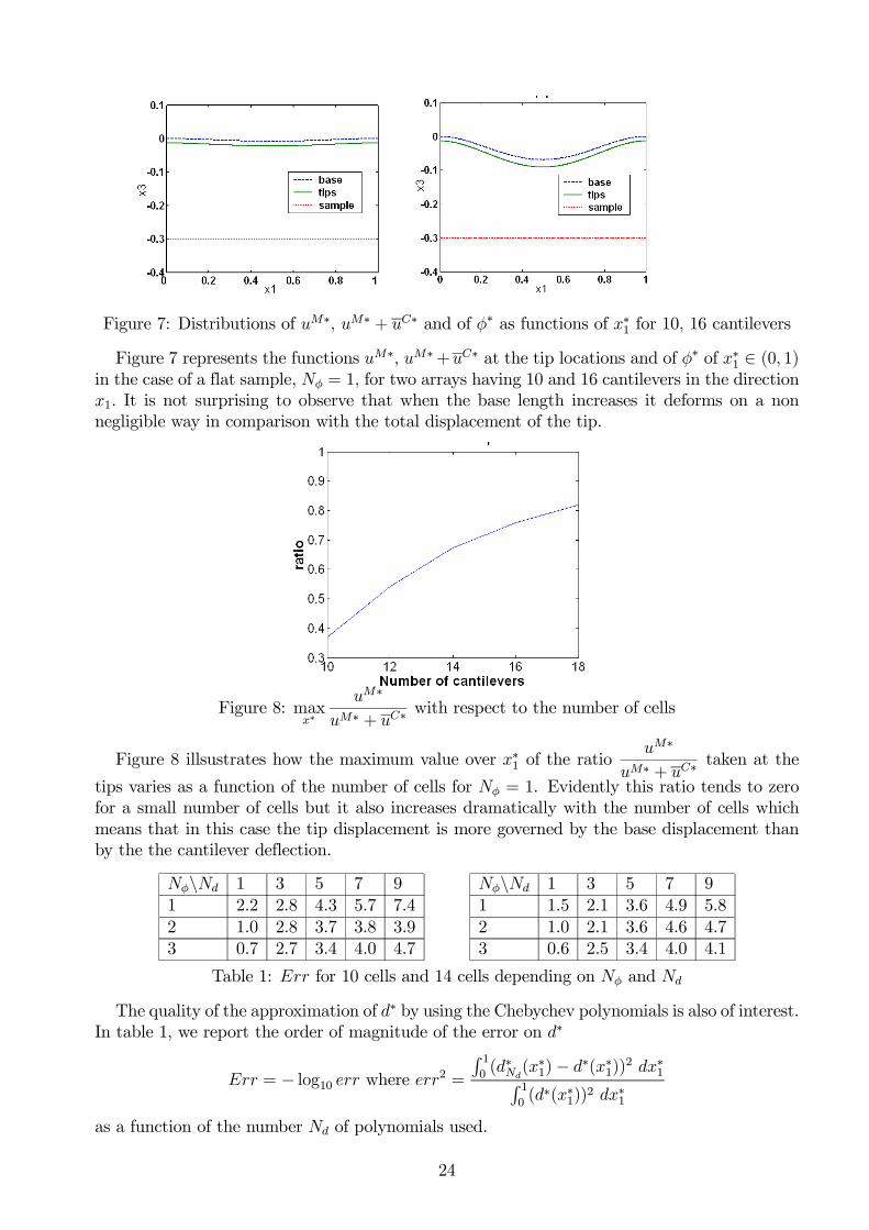
Figure 7: Distributions of uM∗, uM∗ + uC∗ and of φ∗ as functions of x∗1 for 10, 16 cantilevers

Figure 7 represents the functions uM∗, uM∗+uC∗ at the tip locations and of φ∗ of x∗1 ∈ (0, 1)in the case of a flat sample, Nφ = 1, for two arrays having 10 and 16 cantilevers in the directionx1. It is not surprising to observe that when the base length increases it deforms on a nonnegligible way in comparison with the total displacement of the tip.

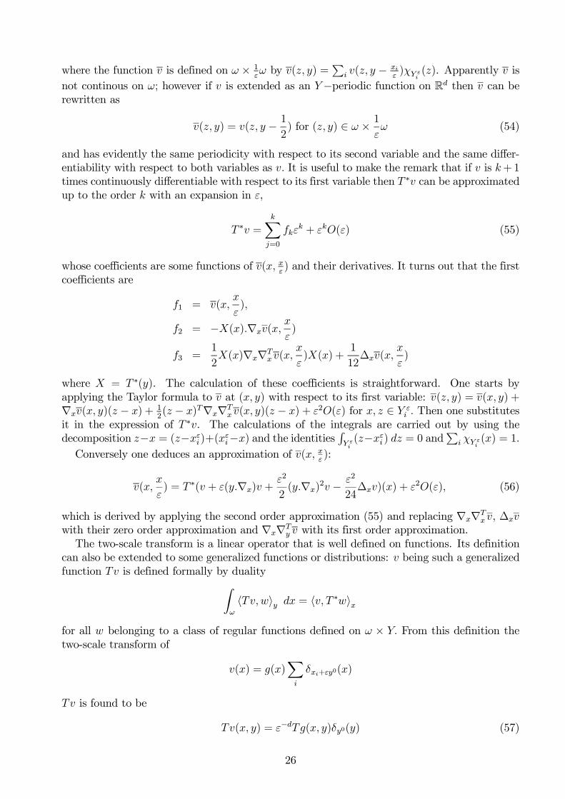
Figure 8: maxx∗

uM∗

uM∗ + uC∗with respect to the number of cells

Figure 8 illsustrates how the maximum value over x∗1 of the ratiouM∗

uM∗ + uC∗taken at the

tips varies as a function of the number of cells for Nφ = 1. Evidently this ratio tends to zerofor a small number of cells but it also increases dramatically with the number of cells whichmeans that in this case the tip displacement is more governed by the base displacement thanby the the cantilever deflection.

Nφ\Nd 1 3 5 7 91 2.2 2.8 4.3 5.7 7.42 1.0 2.8 3.7 3.8 3.93 0.7 2.7 3.4 4.0 4.7

Nφ\Nd 1 3 5 7 91 1.5 2.1 3.6 4.9 5.82 1.0 2.1 3.6 4.6 4.73 0.6 2.5 3.4 4.0 4.1

Table 1: Err for 10 cells and 14 cells depending on Nφ and Nd

The quality of the approximation of d∗ by using the Chebychev polynomials is also of interest.In table 1, we report the order of magnitude of the error on d∗

Err = − log10 err where err2 =R 10(d∗Nd(x

∗1)− d∗(x∗1))2 dx∗1R 1

0(d∗(x∗1))2 dx

∗1

as a function of the number Nd of polynomials used.

24

7 AppendixIn this appendix, we report some mathematical definitions and properties. The concept of weakand strong approximation are defined in Section 7.1. Then in Section 7.2 the two-scale transformof a function is defined and its elementary properties are stated. Weak approximations of firstorder and second order derivatives two-scale derivatives are derived in Section 7.3. In Section7.4 we provide the expression of a volumic force which action is equivalent to a concentratedforce when it is applied in the rigid part. This result is used in the examples of Sections 6.1 and6.2. Finally a fundamental inequality used for the derivation of the two-scale model is statedand proved in Section 7.5.

7.1 Weak and strong Approximation

Consider an open set A ∈ Rn, wε ∈ L2(A), a function depending on the parameter ε anda function w0 ∈ L2(A) independent of ε. We say that wε = w0 + O(ε) weakly in L2(A) ifRA(wε − v0)v dx = O(ε) for all v ∈ L2(A) and we say that the same equality holds strongly in

L2(A) ifRA(wε − w0)2 dx = O(ε).

For example the oscillating function sin(xε) can be approximated by zero in the weak sense

but cannot be approximated by a function independent of ε in the strong sense.

7.2 Properties of the Two-Scale Transform

We state here some elementary properties of the two-scale transform. The proofs are elementaryand are not detailed here. Some may be found in M. Lenczner and G. Senouci [11].For v,w ∈ L1(ω),

\v + w = bv + bw, cvw = bv bw and Zω

v(x)dx =

Zω×Y

bv(x, y)dydxFor v ∈ L2(ω),

||v||ω = ||bv||ω×Yand if ∇v ∈ L2(ω) then

c∇v = ε−1∇ybv.For any εY−periodic part ωx of ω (like ωP ) and Yx its corresponding reference cell in Y , itfollows that

dχωx = χω×Yx.

It is convenient to note that the two scale transform is a linear operator T defined from L2(ω)to L2(ω × Y ) by Tu = bu. Its adjoint T ∗ is defined byZ

ω

u(x)(T ∗v)(x) dx =Zω×Y

(Tu)(x, y)v(x, y) dxdy (53)

for all u ∈ L2(ω) and v ∈ L2(ω × Y ). A direct computation shows that

T ∗v(x) =Xi

ε−dZY εi

v(z,x− xi

ε)dz χY ε

i(x) =

Xi

ε−dZY εi

v(z,x

ε)dz χY ε

i(x)

25

where the function v is defined on ω × 1εω by v(z, y) =

Pi v(z, y − xi

ε)χY ε

i(z). Apparently v is

not continous on ω; however if v is extended as an Y−periodic function on Rd then v can berewritten as

v(z, y) = v(z, y − 12) for (z, y) ∈ ω × 1

εω (54)

and has evidently the same periodicity with respect to its second variable and the same differ-entiability with respect to both variables as v. It is useful to make the remark that if v is k+1times continuously differentiable with respect to its first variable then T ∗v can be approximatedup to the order k with an expansion in ε,

T ∗v =kXj=0

fkεk + εkO(ε) (55)

whose coefficients are some functions of v(x, xε) and their derivatives. It turns out that the first

coefficients are

f1 = v(x,x

ε),

f2 = −X(x).∇xv(x, xε)

f3 =1

2X(x)∇x∇Tx v(x,

x

ε)X(x) +

1

12∆xv(x,

x

ε)

where X = T ∗(y). The calculation of these coefficients is straightforward. One starts byapplying the Taylor formula to v at (x, y) with respect to its first variable: v(z, y) = v(x, y) +∇xv(x, y)(z − x) + 1

2(z − x)T∇x∇Tx v(x, y)(z − x) + ε2O(ε) for x, z ∈ Y ε

i . Then one substitutesit in the expression of T ∗v. The calculations of the integrals are carried out by using thedecomposition z−x = (z−xεi )+(xεi−x) and the identities

RY εi(z−xεi ) dz = 0 and

Pi χY ε

i(x) = 1.

Conversely one deduces an approximation of v(x, xε):

v(x,x

ε) = T ∗(v + ε(y.∇x)v + ε2

2(y.∇x)2v − ε2

24∆xv)(x) + ε2O(ε), (56)

which is derived by applying the second order approximation (55) and replacing ∇x∇Tx v, ∆xvwith their zero order approximation and ∇x∇Ty v with its first order approximation.The two-scale transform is a linear operator that is well defined on functions. Its definition

can also be extended to some generalized functions or distributions: v being such a generalizedfunction Tv is defined formally by dualityZ

ω

hTv, wiy dx = hv, T ∗wix

for all w belonging to a class of regular functions defined on ω × Y. From this definition thetwo-scale transform of

v(x) = g(x)Xi

δxi+εy0(x)

Tv is found to be

Tv(x, y) = ε−dTg(x, y)δy0(y) (57)

26

where y0 ∈ Y , δξ is the Dirac distribution in ξ and g is any regular function. Indeed,

hv, T ∗wix =*g(x)

Xi

δxi+εy0(x),Xj

ε−dZY εj

w(z,x

ε)dz χY ε

j(x)

+x

=Xi

g(xi + εy0)ε−dZY εi

w(z, y0)dz = ε−dXi

ZY εi

Tg(z, y0)w(z, y0)dz

= ε−dZω

Tg(z, y0)w(z, y0)dz = ε−dZω

­Tg(z, y)δy0(y), w(z, y

0)®ydz.

This means that Tv(z, y) = ε−dTg(z, y)δy0(y).

7.3 Approximations of the Two-Scale Transform of the Derivatives

The following results are stated in the general case where d is any positive integer, ω =Πdi=1(0, Li) and Y = (−1

2, 12)d with Li some non negative numbers. The definitions of the

cells Y εi and of the two-scale transform (15) still hold.

Notation: Consider a εY−periodic set ω1 ⊂ ω with cells Y ε1i and the associated unit cell

Y1 =1ε(Y εi − xεi ) ⊂ Y. The intersection between the boundaries of Y1 and of Y is denoted by

γper, it corresponds to the location where the cells Yε1i are connected. We take into account

cases where the cells Y ε1i are connected to their neighbors in some directions but not in the

others. Then the gradient splits in two parts ∇ = ∇C + ∇NC where ∇C and ∇NC containrespectively the partial derivatives in the connectivity directions and in the directions withoutconnectivity. In the same way, the components y and the unit outwards normal vectors n toa boundary (∂ω or ∂Y1) split as y = yC + yNC and n = nC + nNC. The extremal cases wherethe cells Y ε

1i are connected in all directions (∇C = ∇, nC = n and yC = y) or in none ofthem (∇C = nC = yC = 0) are encompassed by these notations. The part of the boundary ∂ωwhere the unit outward normal vector nCx 6= 0 is divided into γM0 where boundary conditionsare applied and γM1 .

First order derivatives: Let u be a function defined on ω1, depending on the parameter ε,vanishing on γM0 ∩ ∂ω1 and such that its norms ||u||ω1 and ||∇u||ω1 are O(1) with respect to ε.From the norm conservation through the two-scale transform, we already know that ||bu||ω×Y1and ||c∇u||ω×Y1 are also O(1). If, in any manner, it is known that bu admits an expansion withrespect to ε on the form bu = u0 + εeu1 + εO(ε), at least in the weak sense, with u0 and eu1independent of ε, then u0 = 0 on γ0, ∇yu0 = 0 on ω × Y1,c∇u = ∇Cx u0 +∇yu1 +O(ε) on ω × Y1 (58)

in the weak sense, u1 = eu1−yC .∇Cx u0, u1 is Y−periodic on γper, u0 ∈ L2(ω), ∇Cx u0(x) ∈ L2(ω)d,

u1 ∈ L2(ω × Y1) and ∇yu1 ∈ L2(ω × Y1)d.Second order derivatives: In addition, we assume that ||∇∇Tu||ω1 is O(1), that ∇u = 0

on γM0 ∩ ∂ω1 and that bu = u0 + εeu1 + εeu2 + ε2O(ε), at least in the weak sense. It then follows

that ||\∇∇Tu||ω×Y1 is O(1), ∇xu0 = 0 on γ0, ∇y∇Ty u1 = 0, ∇Cy u1 = 0,c∇u = ∇Cx u0 + θNC +O(ε) (59)

and \∇∇Tu = ∇Cx (∇Cx )Tu0 +∇Cx (θNC)T + (∇Cx (θNC)T )T +∇∇Tu2 +O(ε)

27

on ω × Y1 in the weak sense, u2 = eu2 − yC .∇Cx eu1 + (yC .∇Cx )2u0, u2 and ∇yu2 are Y−periodicon γper, θ

NC = ∇NCy u1 which is independent of y, ∇Cx (∇Cx )Tu0 ∈ L2(ω)d×d and ∇Cx∇yu1,∇∇Tu2 ∈ L2(ω × Y1)d×d.Strong variations, first order derivatives: In the case where the variations of u are

sufficiently large that ||∇u||ω1 is not of order O(1) but ||ε∇u||ω1 is O(1) and bu = u0 +O(ε), atleast in the weak sense, then ∇yu0 ∈ L2(ω × Y1) and

εc∇u(x, y) = ∇yu0 +O(ε) (60)

in the weak sense.

Strong variations, second order derivatives: If in addition ||ε2∇∇Tu||ω1 is O(1) then∇y∇Ty u0 ∈ L2(ω × Y1) and

ε2\∇∇Tu(x, y) = ∇∇Tu0 +O(ε). (61)

Here we sketch the proof of these approximations by indicating the calculation steps withoutgoing into precise mathematical justifications.

Proof for the first order derivative: The proof is decomposed into four steps.(i) If ||∇u||ω1 is O(1) then ∇yu0 = 0. This comes from the properties of the two-scale

transform recalled above: ε||∇u||ω1 = ε||c∇u||ω×Y1 = ||∇ybu||ω×Y1 = O(ε).Next, we decompose c∇u =[∇Cu+\∇NCu and compute each part separately.(ii) The first term turns out to be approximated by

[∇Cu = ∇Cx u0 +∇Cy u1 +O(ε) on ω × Y1.Consider a function v(x, y) two times continuously differentiable with respect to x in ω × Y1,vanishing for y ∈ ∂Y1 − γper and for x ∈ γM1 and extended by zero for y ∈ Y − Y1. We assumealso that the function v defined from v by (54) is differentiable with respect to y. Then, Eω1

denoting the operator of extension by zero from ω1 to ω,

X =

Zω×Y

TEω1∇Cu.v dydx =Zω1

∇Cu.T ∗v dx =Zω1

∇Cu(x).v(x, xε) dx+O(ε)

due to the zero order approximation of T ∗v and the fact that ||∇u||ω1 is bounded. Applyingthe Green formula and taking into account that the product u v vanishes on the boundary ofω it follows that

X = −Zω1

u(x)(divCx v(x,x

ε) + ε−1divCy v(x,

x

ε)) dx+O(ε).

Applying the approximation (55) at the zero order to divCx v(x,xε) and at the first order to

divCy v(x,xε) yields

X = −Zω1

u T ∗(divCx v + ε−1divCy v + y.∇xdivCy v) dx+O(ε)

or equivalently

X = −Zω×Y1

bu (divCx v + ε−1divCy v + y.∇xdivCy v) dxdy +O(ε)

28

Since bu = u0 + εeu1 + εO(ε) and ∇Cy u0 = 0, applying the Green formula in the reverse senseyields Z

ω×Y[∇Cu.v dydx =

Zω×Y1

(∇Cx u0 +∇Cy u1).v dydx (62)

−Zω×γper

u1v.nCy ds(y)dx−ZγM0 ×Y1

u0v.nCx ds(y)dx+O(ε)

with u1 = eu1 − yC .∇Cx u0. From the conditions imposed on v, it follows that all the boundaryterms except those on ω × γper vanish. Here we have used the fact that

RY1u0 yNC .∇xdivCy v

dy = 0. Reducing the choice of functions to those satisfying v = 0 on ω × γper and on γM0 × Y1gives Z

ω×Y[∇Cu.v dydx =

Zω×Y1

(∇Cx u0 +∇Cy u1).v dydx+O(ε)

which holds only for the above mentioned v. However, from a density argument this is valid

also for all v ∈ L2(ω×Y1). So we conclude that the equality[∇Cu = ∇Cx u0+∇Cy u1+O(ε) holdsin the weak sense.

(iii) As a by-product of (62) it follows that u1 is Y−periodic on γper and u0 = 0 on γM0 .

Restarting from (62) with v = 0 on γM0 × Y1 it follows thatZω×γper

u1v.nCy ds(y)dx = O(ε)

which says that u1 is Y−periodic on γper. Finally for an v it remainsZγM0 ×Y1

u0v.nCx ds(y)dx = O(ε)

that says that u0 = 0 on γM0 .

(iv) The expression of the complementary \∇NCu is\∇NCu = ∇NCy u1 +O(ε).

Indeed \∇NCu = ε−1∇NCy bu = ε−1∇NCy (u0 + εeu1) +O(ε) = ∇NCy u1 +O(ε).This completes the derivation of (58).

Sketch of the proof for the second order derivative: From ||∇∇Tu||ω1 = O(1) it followsthat ∇y∇Ty u1 vanishes, then u1 is affine with respect to y and θNC = ∇NCy u1 is independentof y. Furthermore, u1 being periodic on γper implies that it is independent of y

C or in otherwords that ∇Cy u1 = 0. The proof of (59) follows the same arguments (58) except that v is asymmetric d× d matrix. The matrix of second order derivative splits in three parts ∇∇Tu =(∇C)2u+∇C(∇NC)Tu+∇NC(∇C)Tu+ (∇NC)2u.(i) The approximation of the first term

\∇C(∇C)Tu = ∇Cx (∇Cx )Tu0 +∇Cy (∇Cy )Tu2 +O(ε) on ω × Y1 (63)

29

and of the boundary conditions on γM0 and on γper are derived through the same calculation.The second order approximation (55) of T ∗v leads, after few lines of simple calculation, toZ

ω×Y\∇C(∇C)Tu : : v dydx =

Zω×Y1

(∇Cx (∇Cx )Tu0 +∇Cy (∇Cy )Tu2) :: v dydx

+

Zω×γper

[u1(divCx v) + u2(divCy v)− (∇Cy u2)Tv].nCy ds(y)dx+O(ε).

The formula (63) as well as the boundary conditions follow.

(ii) The second term \∇C∇NCu is approximated by\∇C(∇NC)Tu = ∇Cx (θNC)T +∇NCy (∇Cy )Tu2 +O(ε). (64)

Here ∇NC is applied to u and ∇C is transposed on the test function. Following the calculationand using the fact that ∇NCy (yC .∇Cx u0) = 0 the formulaZ

ω×Y\∇C(∇NC)Tu :: vdydx =

Zω×Y1

(∇Cx (θNC)T +∇NCy (∇Cy )Tu2) :: v dydx+O(ε)

arises when v = 0 on ω × γper and on ∂ω × Y1. This provides immediately (64).(iii) The third term \∇NC(∇C)Tu is equal to the second term transposed so its approximation

is equal to the transposed approximation of the second term.(iv) The derivation of the formula for the fourth term

\(∇NC)2u = ∇NCy (∇NCy )Tu2 +O(ε) on ω × Y1 (65)

is straightforward.

Proof for the strong variations case: For proving (60) and (61), let us recall that

εc∇u = ∇ybu and ε2\∇∇Tu = ∇y∇Ty bu, so using the expansion of bu leads directly to the results.7.4 The volumic force associated to a concentrated force in the rigid

part

Consider a concentrated force F δxtip(x) applied to the extremity of the rigid part ΩR in theexample 6.1 where F is any vector of R3. We may prove that the force

f(x) =F

|ΩR| + F × (x− xG)

produces the same effect on the rigid part as the concentrated force where xG is the gravitycenter of ΩR and F = A−1((xtip − xG)× F ). The associated forces in the plate model are

fP (x) =a+ h(x)

|ΩR| [F3 + F .(x2,−x1, 0)T ]

gP1 (x) =a2 − h2(x)2|ΩR| F2 + F .(0, a− h(x)

2,−x2)T

gP2 (x) =a2 − h2(x)2|ΩR| F2 + F .(−a− h(x)

2, 0,−x1)T .

30

We remark that, if F is colinear to xtip − xG then F = 0. Furthermore if F = (0, 0, F3)T theforces in the thin plates are

fP (x) =a+ h(x)

|ΩR| F3 and gPα = 0.

Here A is the 3× 3 matrice with coefficients

Aii =Xj 6=i

ZΩR

(xj − xGj )2 dx and Aij = −ZΩ

(xi − xGi )(xj − xGj ) dx for i 6= j.

To prove this, one search the function f under the form f(x) = d +D × (x − xG) with d andD in R3 which satisfies Z

ΩR

f(x)v(x) dx = F.v(x0)

for v(x) = c+C × (x− xG) and all c and C in R3. By posing C = 0 it follows that d = F/|ΩR|and then by posing c = 0 :Z

ΩR

(C × (x− xG)).(D × (x− xG)) dx = (C × (x0 − xG)).F

or equivalently

C.

ZΩR

(x− xG)× (D × (x− xG)) dx = C.((x0 − xG)× F )

then ZΩR

(x− xG)× (D × (x− xG)) dx = (x0 − xG)× F

from which the expression D = A−1((x0 − xG)× F ) follows. The expressions of fP and gP arederived straightfowardly.

7.5 An Inequality

Lemma 2 For all v ∈ H1(ωP ) such that v = 0 on γε0 it follows that

||v||ωP ≤ C||χωB∇v + χωF

ε∇v||ωP . (66)

Proof. (i) First we establish that there exists a constant C1 > 0 such that for all v ∈ H1(Y )||v||2YC ≤ C1(||v||2YB + ||∇v||2Y ). This is proven similarly to the classical Poincaré inequalities.(ii) Then we establish that there exists a constant C2 > 0 such that for all v ∈ H1

γε0(ωP ) and

all ε > 0, ||v||2ωP ≤ C3||χωB(∂x1v, ε∂x2v) + ε∇v||2ωP . Let us start from the previous inequality

and for each i let us apply the change of variable that maps Y towards Y εi for each. This leads

to a family of inequality that we sum over i. It follows that for all v ∈ H1(ωP ) :

||v||2ωC ≤ C1(||v||2ωC + ||ε∇v||2ωP ). (67)

By another way, let us introduce a scaling of ωB by a factor of n = 1/ε in the direction x2only. This leads to a family bω of n strips with length equal to 1 in the x1 direction and of the

31

order of one in the second direction. The classical Poincaré inequality may be applied to eachof them which in turn by summation over the n strips yields ||v||2bω ≤ C2||∇v||2bω provided thatv ∈ H1bγε0(bωε). Here bγε0 is obtained through the dilatation of γε0 by a factor 1/ε. By reversing thescaling, it follows that for all v ∈ H1

γε0(ω),

||v||2ωC ≤ C2||(∂x1v, ε∂x2v)||2ωC . (68)

Combining (67-68) yields (ii)(iii) The desired result is a direct consequence of (ii).

Conclusion: We have derived two-scale models of AFM Arrays which take into accountthe deformations of the base coupled with those of the cantilevers. The first model is a generalone and can be discretized with a Finite Element Method for both the macroscopic domainand the reference cell. The second model is a particular case where hand calculations havebeen pushed at their limit, so it has the form of a Euler Bernoulli beam equation, associated tothe base, coupled with a nonlinear algebraic equation for the cantilevers. They do not requirean heavy Finite Elements implementation and may provide an efficient model for a designer.The derivation of the general model is based on asymptotic approach which guaranties a goodconfidence in its results. Let us review the features of the general model. The cantileversare modeled with a Love-Kirchhoff thin plate model which allows to describe general plateflexions encountered for example in nanomanipulation, their tip is rigid, the atomic forces arereally applied to the extremity of the tip and the base is assumed to be much stiffer than thecantilevers which simplifies significantly the model. The results show that even for a smallnumber of cantilevers, the mechanical displacement of the base cannot be neglected in a designprocess. Our perspectives consist in completing this work by several aspects including thedynamics, realistic shapes of the sample and control of the whole system.

References[1] Destuynder, P.; Salaun, M.. Mathematical analysis of thin plate models, Springer, Berlin,

1996.

[2] Ciarlet, P.G.. Mathematical elasticity. Vol. II, North-Holland, Amsterdam, 1997.

[3] Sanchez-Palencia, E.. Nonhomogeneous media; vibration theory, Lecture Notes in Phys.,127, Springer, Berlin, 1980.

[4] Bensoussan, A; Lions, J-L; Papanicolaou, G.. Asymptotic analysis for periodic structures,North-Holland, Amsterdam, 1978.

[5] Allaire, G.. SIAM J. Math. Anal., v 23 (1992), n 6, 1482-1518.

[6] Canon, E.; Lenczner, M.. Math. Comput. Modelling, v 26 (1997), n 5, 79-106.

[7] Nguetseng, G.. SIAM J. Math. Anal., v 20 (1989), n 3, 608-623.

[8] Cioranescu, D.; Damlamian, A.; Griso, G.. C. R. Math. Acad. Sci. Paris, v 335 (2002), n1, 99-104.

[9] Casado-Diaz, J.. Two-scale convergence for nonlinear Dirichlet problems in perforateddomains. Proc. Roy. Soc. Edinburgh Sect. A, v 130, (2000), n 2, 249276.

32

[10] Lenczner, M.; Mercier, D.. Multiscale Model. Simul. v 2 (2004), n 3, 359-397.

[11] Lenczner, M.; Senouci-Bereksi, G.. Math. Models Methods Appl. Sci., v 9 (1999), n 6,899-932.

[12] Fung R.F.; Huang S.. Dynamic modeling; vibration analysis of the atomic force microscope.Transactions of the ASME. Journal of Vibration; Acoustics, v 123, n 4, (2001), p 502-9.

[13] Drakova, D.. Theoretical modelling of scanning tunnelling microscopy, scanning tunnellingspectroscopy; atomic force microscopy. Reports on Progress in Physics, v 64, n 2, (2001),p 205-90.

[14] Giessibl, F.J.. Advances in atomic force microscopy. Reviews of Modern Physics, v 75, n3, (2003), p 949-83.

[15] Lenczner, M.. Homogenization of an electric circuit. Comptes Rendus de l0Academie desSciences, Serie II, v 324, n 9, (1997), p 537-42.

[16] Stark, R.W.; Schitter, G.; Stark, M.; Guckenberger, R.; Stemmer, A. State-space modelof freely vibrating and surface-coupled cantilever dynamics in atomic force microscopy.Physical Review B (Condensed Matter and Materials Physics), v 69, n 8, (2004), p 85412-1-9.

[17] Gotsmann, B., Seidel, C.; Anczykowski, B.; Fuchs, H. Conservative and dissipative tip-sample interaction forces probed with dynamic AFM. Physical Review B (Condensed Mat-ter), v 60, n 15, (1999), p 11051-61.

[18] Vinogradova, O.I., Butt, H.-J.; Yakubov, G.E.; Feuillebois, F. Dynamic effects on forcemeasurements. I. Viscous drag on the atomic force microscope cantilever. Review of Sci-entific Instruments, v 72, n 5, (2001), p 2330-9.

[19] Lobontiu, N.; Garcia, E. Two microcantilever designs: lumped-parameter model for staticand modal analysis. Journal of Microelectromechanical Systems, v 13, n 1, (2004), p 41-50.

[20] Jalili, N.; Dadfarnia, M.; Dawson, D.M. A fresh insight into the microcantilever-sampleinteraction problem in non-contact atomic force microscopy. Transactions of the ASME.Journal of Dynamic Systems, Measurement and Control, v 126, n 2, (2004), p 327-35.

[21] Garcia, R.; Perez, R. Dynamic atomic force microscopy methods. Surface Science Reports,v 47, n 6-8, (2002), p 197-301.

[22] Elmer, F.-J.; Dreier, M. Eigenfrequencies of a rectangular atomic force microscope can-tilever in a medium. Journal of Applied Physics, v 81, n 12, 15 June (1997), p 7709-14.

[23] Sader, J.E. Frequency response of cantilever beams immersed in viscous fluids with appli-cations to the atomic force microscope. Journal of Applied Physics, v 84, n 1, 1 (1998), p64-76.

[24] Napoli, M.; Wenhua Zhang; Turner, K.; Bamieh, B. Characterization of electrostaticallycoupled microcantilevers. Journal of Microelectromechanical Systems, v 14, n 2, (2005), p295-304. A capacitive microcantilever: modelling, validation, and estimation using currentmeasurements.

33

[25] Napoli, M.; Bamieh, B.; Dahleh, M. Optimal control of arrays of microcantilevers. Trans-actions of the ASME. Journal of Dynamic Systems, Measurement and Control, v 121, n4, (1999), p 686-90.

[26] Argento, C. and French, R.H. Parametric tip model and forcedistance relation forHamaker constant determination from atomic force microscopy, Journal of Applied Physics,v 11, n 1, (1996), p 6081-6090.

[27] Argento, C., Jagota, A., and Carter, W.C., Surface formulation for molecular interactionsof macroscopic bodies, Journal of the Mechanics and Physics of Solids, v 45, n 7, (1997),p 1161-1183.

[28] J. Israelachvili, Intermolecular and Surface Forces: Second Edition, Academic Press, Lon-don, 1992.

[29] Lang, H. P.; Hegner, M.; Gerber, C. Cantilever array sensors. Materials Today, v 8, n 4,(2005), p 30-36.

[30] Fasching, R. J.; Tao, Y.; Prinz, F. B.. Cantilever tip probe arrays for simultaneous SECMand AFM analysis. Sensors and Actuators, B: Chemical, v 108, n 1-2, (2005), p 964-972.

[31] Nugaeva, N.; Gfeller, K. Y.; Backmann, N.; Lang, H. P.; Duggelin, M.; Hegner, M. Mi-cromechanical cantilever array sensors for selective fungal immobilization and fast growthdetection. Biosensors and Bioelectronics, v 21, n 6, Dec 15, 2005, p 849-856.

[32] Volden, T.; Zimmermann, M.; Lange, D.; Brand, O.; Baltes, H.. Dynamics of CMOS-based thermally actuated cantilever arrays for force microscopy. Sensors and Actuators,A: Physical, v 115, n 22, (2004), p 516-52.

[33] Xu, T.; Bachman, M.; Zeng, F.; Li, G.. Polymeric micro-cantilever array for auditoryfront-end processing. Sensors and Actuators, A: Physical, v 114, n 2-3,(2004), p 176-182.

[34] Yang, Z.; Li, X.; Wang, Y.; Bao, H.; Liu, M.. Micro cantilever probe array integrated withPiezoresistive sensor. Microelectronics Journal, v 35, n 5, (2004), p 479-483.

[35] Kim, Y.; Nam, H.; Cho, S.; Hong, J.; Kim, D.; Bu, J. U.. PZT cantilever array integratedwith piezoresistor sensor for high speed parallel operation of AFM. Sensors and Actuators,A: Physical, v 103, n 1-2, (2003), p 122-129.

[36] Saya, D.; Fukushima, K.; Toshiyoshi, H.; H., G.; Fujita, H.; Kawakatsu, H.. Fabrication ofsingle-crystal Si cantilever array. Sensors and Actuators, A: Physical, v 95, n 2-3, (2002),p 281-287.

[37] Kim, B.H.; Prins, F.E.; Kern, D.P.; Raible, S.; Weimar, U.. Multicomponent analysis andprediction with a cantilever array based gas sensor. Sensors and Actuators, B: Chemical,v 78, n 1-3, (2001), p 12-18.

[38] Battiston, F.M.; Ramseyer, J.-P.; Lang, H.P.; Baller, M.K.; Gerber, C.; Gimzewski, J.K.;Meyer, E.; Guntherodt, H.-J.. A chemical sensor based on a microfabricated cantileverarray with simultaneous resonance-frequency and bending readout. Sensors and Actuators,B: Chemical, v 77, n 1-2, (2001), p 122-131.

34

[39] Chow, E.M.; Soh, H.T.; Lee, H.C.; Adams, J.D.; Minne, S.C.; Yaralioglu, G.; Atalar,A.; Quate, C.F.; Kenny, T.W.. Integration of through-wafer interconnects with a two-dimensional cantilever array. Sensors and Actuators A (Physical), v A83, n 1-3, (2000), p118-23.

[40] Rudnitsky, R.G.; Chow, E.m.; Kenny, T.W.. Rapid biochemical detection and differentia-tion with magnetic force microscope cantilever arraysSensors and Actuators A (Physical),v A83, n 1-3, (2000), p 256-62.

[41] Baller, M.K.; Lang, H.P.; Fritz, J.; Gerber, Ch.; Gimzewski, J.K.; Drechsler, U.; Rothuizen,H.; Despont, M.; Vettiger, P.; Battiston, F.M.; Ramseyer, J.P.; Fornaro, P.; Meyer,E.; Guntherodt, H.-J.. Cantilever array-based artificial nose. Ultramicroscopy, v 82, n1, (2000), p 1-9.

[42] Lutwyche, M.; Andreoli, C.; Binnig, G.; Brugger, J.; Drechsler, U.; Haberle, W.; Rohrer,H.; Rothuizen, H.; Vettiger, P.; Yaralioglu, G.; Quate, C.. 5×5 2D AFM cantilever arraysa first step towards a Terabit storage device. Sensors and Actuators A (Physical), v A73,n 1-2, (1999), p 89-94;

[43] Young-Sik Kim; Sunyong Lee, C.; Won-Hyeog Jin; SeongSoo Jang; Hyo-Jin Nam; Jong-UkBu. 100×100 thermo-piezoelectric cantilever array for SPM nano-data-storage application.Sensors and Materials, v 17, n 2, (2005), p 57-63.

[44] Kakushima, K.; Watanabe, T.; Shimamoto, K.; Gouda, T.; Ataka, M.; Mimura, H.; Isono,Y.; Hashiguchi, G.; Mihara, Y.; Fujita, H.. Japanese Journal of Applied Physics, v 43, n6B, (2004), p 4041-4.

[45] Graf, M.J.; Opeil, C.P.; Huber, T.E.. Magnetic anisotropy and de Haas-van Alphen oscil-lations in a Bi microwire array studied via cantilever magnetometry at low temperatures.Journal of Low Temperature Physics, v 134, n 5-6, (2004), p 1055-68.

[46] Yu Xiaomei; Zhang Dacheng; Li Ting; Wang Xiaobao; Ruan Yong; Du Xianfeng. Fabrica-tion and analysis of micromachined cantilever array. Chinese Journal of Semiconductors,v 24, n 8, (2003), p 861-5.

[47] Srinivasan, P.; Beyette, F.R., Jr.; Papautsky, I.. Micromachined arrays of cantileveredglass probesd. Applied Optics, v 43, n 4, (2004), p 776-82.

[48] Bullen, D.; Sung-Wook Chung; Xuefeng Wang; Jun Zou; Mirkin, C.A.; Chang Liu. Par-allel dip-pen nanolithography with arrays of individually addressable cantilevers. AppliedPhysics Letters, v 84, n 5, (2004), p 789-91.

[49] Calleja, M.; Tamayo, J.; Johansson, A.; Rasmussen, P.; Lechuga, L.M.; Boisen, A.. Poly-meric cantilever arrays for biosensing applications. Sensor Letters, v 1, n 1, (2003), p20-4.

[50] Abedinov, N.; Popov, C.; Yordanov, Z.; Ivanov, T.; Gotszalk, T.; Grabiec, P.; Kulisch, W.;Rangelow, I.W.; Filenko, D.; Shirshov, Yu.. Chemical recognition based on micromachinedsilicon cantilever array. Journal of Vacuum Science; Technology B, v 21, n 6, (2003), p2931-6.

[51] Dragoman, D.; Dragoman, M.. Biased micromechanical cantilever arrays as optical imagememory. Applied Optics, v 42, n 8, (2003), p 1515-19.

35

[52] Arntz, Y.; Seelig, J.D.; Lang, H.P.; Zhang, J.; Hunziker, P.; Ramseyer, J.P.; Meyer, E.;Hegner, M.; Gerber, C.. Label-free protein assay based on a nanomechanical cantileverarray. Nanotechnology, v 14, n 1, (2003), p 86-90.

[53] Schaffer, T. E.. Force spectroscopy with a large dynamic range using small cantilevers andan array detector. Journal of Applied Physics, v 91, n 7, (2002), p 4739.

[54] Abedinov, N.; Grabiec, P.; Gotszalk, T.; Ivanov, Tz.; Voigt, J.; Rangelow, I.W.. Microma-chined piezoresistive cantilever array with integrated resistive microheater for calorimetryand mass detection. Journal of Vacuum Science and Technology, Part A: Vacuum, Surfacesand Films, v 19, n 6, (2001), p 2884-2888.

[55] Cheng, H.-M.; Ewe, M.T.S.; Chiu, G.T.-C.; Bashir, R.. Modeling and control of piezo-electric cantilever beam micro-mirror and micro-laser arrays to reduce image banding inelectrophotographic processes. Journal of Micromechanics and Microengineering, v 11, n5, (2001), p 487-98.

[56] Green, J. D.; Lee, G. U.. Atomic force microscopy with patterned cantilevers and tip arrays:Force measurements with chemical arrays. Langmuir, v 16, n 8, (2000), p 4009-4015.

[57] Min Y. ; Lin, H.; Dedrick, D.E.; Satyanarayana, S.; Majumdar, A.; Bedekar, A.S.; Jenkins,J.W.; Sundaram, S.. A 2-D microcantilever array for multiplexed biomolecular analysis.Journal of Microelectromechanical Systems, v 13, n 2, (2004), p 290-9.

[58] Drechsler, U.; Burer, N.; Despont, M.; Durig, U.; Gotsmann, B.; Robin, F.; Vettiger, P..Cantilevers with nano-heaters for thermomechanical storage application. MicroelectronicEngineering, v 67-68, (2003), p 397-404.

[59] Tian, F.; Hansen, K. M.; Ferrell, T. L.; Thundat, T.; Hansen, D. C.. Dynamic microcan-tilever sensor for discerning biomolecular interactions. Analytical Chemistry, v 77, n 6,(2005), p 1601-1606.

[60] Hansen, K.M.; Ji, H.-F.; Wu, G.; Datar, R.; Cote, R.; Majumdar, A.; Thundat, T..Cantilever-based optical deflection assay for discrimination of DNA single-nucleotide mis-matches. Analytical Chemistry, v 73, n 7, (2001), p 1567-1571.

[61] Pepper, J.; Noring, R.; Klempner, M.; Cunningham, B.; Petrovich, A.; Bousquet, R.;Clapp, C.; Brady, J.; Hugh, B.. Detection of proteins and intact microorganisms usingmicrofabricated flexural plate silicon resonator arrays. Sensors and Actuators, B: Chemical,v 96, n 3, (2003), p 565-575.

[62] King, W. P.; Kenny, T. W.; Goodson, K. E.; Cross, G. L.W.; Despont, M.; Durig, U. T.;Rothuizen, H.; Binnig, G.; Vettiger, P.. Design of atomic force microscope cantilevers forcombined thermomechanical writing and thermal reading in array operation. Journal ofMicroelectromechanical Systems, v 11, n 6, (2002), p 765-774.

36