A Two Factor Forward Curve Model with Stochastic ...

A Two Factor Forward Curve Model with

Stochastic Volatility for Commodity Prices

Mark Higgins, PhD - Beacon Platform Incorporated

August 10, 2017

Abstract

We describe a model for evolving commodity forward prices that in-corporates three important dynamics which appear in many commoditymarkets: mean reversion in spot prices and the resulting Samuelson effecton volatility term structure, decorrelation of moves in different points onthe forward curve, and implied volatility skew and smile.

This model is a “forward curve model” - it describes the stochasticevolution of forward prices - rather than a “spot model” that modelsthe evolution of the spot commodity price. Two Brownian motions drivemoves across the forward curve, with a third Heston-like stochastic volatil-ity process scaling instantaneous volatilities of all forward prices.

In addition to an efficient numerical scheme for calculating Euro-pean vanilla and early-exercise option prices, we describe an algorithmfor Monte Carlo-based pricing of more generic derivative payoffs whichinvolves an efficient approximation for the risk neutral drift that avoidshaving to simulate drifts for every forward settlement date required forpricing.

1 The Model Dynamics

Forward price dynamics in commodities markets are often more complex thanin traditional financial markets because the usual spot versus forward arbitragecannot be implemented. The usual expression for a fair forward price in financialmarkets is

F (t, T ) = S(t)e(R−Q)(T−t) (1)

where F (t, T ) is the forward price for settlement at time T , as seen at cal-endar time t; S(t) is the asset spot price at t, R is the denominated currencydiscount rate, and Q is the asset yield.

This expression holds only when two conditions are met: the asset can bestored, and the asset can be borrowed and shorted - both at a capacity com-parable to the size of the market. This is the case for financial markets like

1

arX

iv:1

708.

0166

5v2

[q-

fin.

PR]

8 A

ug 2

017

equities, foreign exchange, and precious metals, but fails to hold for most phys-ical commodity market such as oil, natural gas, and electricity.

If those conditions do hold then forward prices for different settlement datestend to move with close to 100% correlation, because any market forward pricethat deviated from the fair forward price would be arbitraged back into line. Ifthese two conditions fail to hold, however, then forward prices can move relativeto each other with less than a 100% correlation since arbitrage does not forcethem to move together.

Models for commodity price evolution typically fall into two categories: mod-els of the spot price and convenience yield Q (for example [1] and [2]) and mod-els of the forward prices themselves (for example [3] and [4]). Since commoditymarkets usually trade in forward price terms, through futures markets and over-the-counter forward transactions, the latter category of model - called “forwardcurve” models - is often more intuitive for derivatives traders. Forward curvemodels are similar to interest rate models like the LIBOR Market Model [5].

In addition to decorrelation of moves in forward prices, the absence of thetwo conditions required to implement the spot versus forward arbitrage alsomeans that the risk neutral drift of the commodity spot price is not forced to beequal to the difference in two interest rates, and the risk neutral drift can havea more complicated structure. In particular, commodity markets exhibit meanreversion in spot prices [6], and that real-world mean reversion can bleed intorisk neutral pricing. Mean reversion in spot prices means that the instantaneousvolatility of forward prices with longer settlement times tends to be smallerthan instantaneous volatility of forward prices with shorter settlement times(the Samuelson effect, see [7]).

Decorrelation of forward price moves and mean reversion are two importantdynamics to incorporate in any model of commodity forward price evolution.For example, the Gabillon model [3] is a two-factor forward curve model thatincorporates both dynamics, and leads to lognormally-distributed forward priceswith a term structure of implied volatility that can closely match at-the-moneymarket option prices. A lognormal distribution of forward prices gives impliedvolatilities that are constant as a function of strike for a given expiration date,however, and real commodity markets exhibit significant implied volatility skewand smile.

The model defined in this paper adds one-factor stochastic volatility tothe modeled dynamics, following a similar approach to the well known Hestonstochastic volatility model, which generalizes a spot price model with stochasticvolatility [8]. This generalization lets us model market implied volatility skewand smile in addition to the volatility term structure.

2 The Model Definition

Our model for evolution of a forward price F (t, T ) is given by the set of stochasticdifferential equations

2

dF (t, T )

F (t, T )=

√v(t)σ

(e−β1(T−t)dz1(t) +Re−β2(T−t)dz2(t)

)dv(t) = β(1− v(t))dt+ α

√v(t)dz3(t)

E[dz1(t)dz2(t)] = ρdt

E[dz1(t)dz3(t)] = ρ1dt

E[dz2(t)dz3(t)] = ρ2dt (2)

That is: forward prices across the forward curve (all different values of Tfor a given calendar time t) are driven by only two Brownian motions, and theimpact of each Brownian motion shock is different for different values of T ,leading to an instantaneous volatility that tends to decline with T due to theconstant mean reversions β1 and β2 that model the observed Samuelson effect.

The two forward curve shocks are correlated with a constant correlation ρ,and that lack of perfect correlation means that moves in forwards for differentvalues of T are not 100%, allowing us to model the observed decorrelation offorward price moves.

Finally, the instantaneous volatility of all forward prices is scaled by theHeston factor v(t), which is unitless and is order 1. We further specify theinitial condition of v(0) = 1, so that volatility term structure is mostly specifiedthrough the constant model parameters σ, β1, β2, R, and ρ. The constantmean reversion speed of the volatility factor, β, and the constant volatility ofvolatility parameter α, define the term structure of implied volatility smile. Thecorrelation of volatility factor with first forward curve factor ρ1, and with secondforward curve factor ρ2, define the term structure of implied volatility skew.

3 Vanilla and Early Exercise Option Pricing

“Vanilla” European options are ones where the expiration time te of the optionmatches the settlement time of the underlying forward contract T . An “earlyexercise” option is also a European option on a forward settling at time T , butthe option expires at an earlier time te ≤ T , exercising into the underlyingforward contract when in the money at te. Since vanilla options are a subset ofearly exercise options, in this section we derive pricing for early exercise options.

The approach is similar to that for pricing vanilla options under the originalHeston model [8]: first we calculate the characteristic function of the log-forwardprice on the expiration time; then we integrate a function including that char-acteristic function to calculate an option price.

Unlike the standard Heston model, the characteristic function cannot becalculated in closed form: one numerical integration is required. Since we needanother numerical integration to get an option price, this method imples atwo-dimensional numerical integration to price early exercise options, ratherthan a one-dimensional numerical integration for the original Heston model. Atwo-dimensional numerical integration is still significantly more computationally

3

efficient than other numerical techniques for pricing options, such as backwardinduction through a finite difference grid or Monte Carlo simulation.

We start by changing variable to x(t, T ) = ln (F (t, T )/F (0, T )). Then

dx = −v(t)

2σ2F (t, T )dt+

√v(t)σ

(e−β1(T−t)dz1(t) +Re−β2(T−t)dz2(t)

)(3)

where σ2F (t, T ) is the determinstic part of the instantaneous volatility:

σ2F (t, T ) = σ2

(e−2β1(T−t) +R2e−2β2(T−t) + 2ρRe−(β1+β2)(T−t)

)(4)

We define the characteristic function f as

f(x(t, T ), v(t); θ) = E[eiθx(te,T )] (5)

where the expectation E[...] is under the risk neutral measure, t is the currentcalendar time, te is the expiration time of the early exercise option, and T isthe settlement date of the underlying forward.

Since we are considering only one settlement time T in the pricing of earlyexercise options, going forward in this section we will drop the T from x(t, T )and write it simply as x(t).

If we apply Ito’s Lemma to f and set its drift to zero (because f is a mar-tingale in the risk neutral measure) we get a partial differential equation that fsatisfies:

vσ2F (t, T )

2(∂2f

∂x2− ∂f

∂x) + β(1− v)

∂f

∂v+α2v

2

∂2f

∂v2

+σαv(e−β1(T−t)ρ1 +Re−β2(T−t)ρ2)∂2f

∂x∂v+∂f

∂t= 0 (6)

The next step is to try a solution of the form

f(x(t), v(t); θ) = eiθx(t)+A(t)+B(t)v(t) (7)

where A and B are functions only of calendar time t. Also, we change thecalendar time variable to τ = te − t, so that the boundary condition at τ = 0 isA = B = 0.

In the usual way this reduces the partial differential equation to a pair ofordinary differential equations:

dA

dτ= βB

dB

dτ= −1

2(θ2 + iθ)σ2

F (t, T )− βB +α2

2B2

+ iθBασ(e−β1τe−β1(T−te)ρ1 +Re−β2τe−β2(T−te)ρ2) (8)

4

Unlike the standard Heston model we know of no closed form solution tothis pair of ordinary differential equations; instead they can be numerically in-tegrated using standard numerical techniques for integrating first-order ordinarydifferential equations. Along with the initial conditions A(τ = 0) = B(τ = 0) =0, we can calculate A and B for any τ , and thereby calculate the characteristicfunction f .

The next step is to calculate a vanilla option price from the characteristicfunction. As usual, the call price C(K) for strike K is given by

C(K) = D(T )(F (0, T )− K

2− K

π

∫ ∞θ=0

<[f(θ)e−iθ lnK/F (0,T )

θ2 + iθ]) (9)

where D(T ) is the discount factor to settlement time T . Put prices can becalculated from call prices using put/call parity, of course, as these are Europeanoptions.

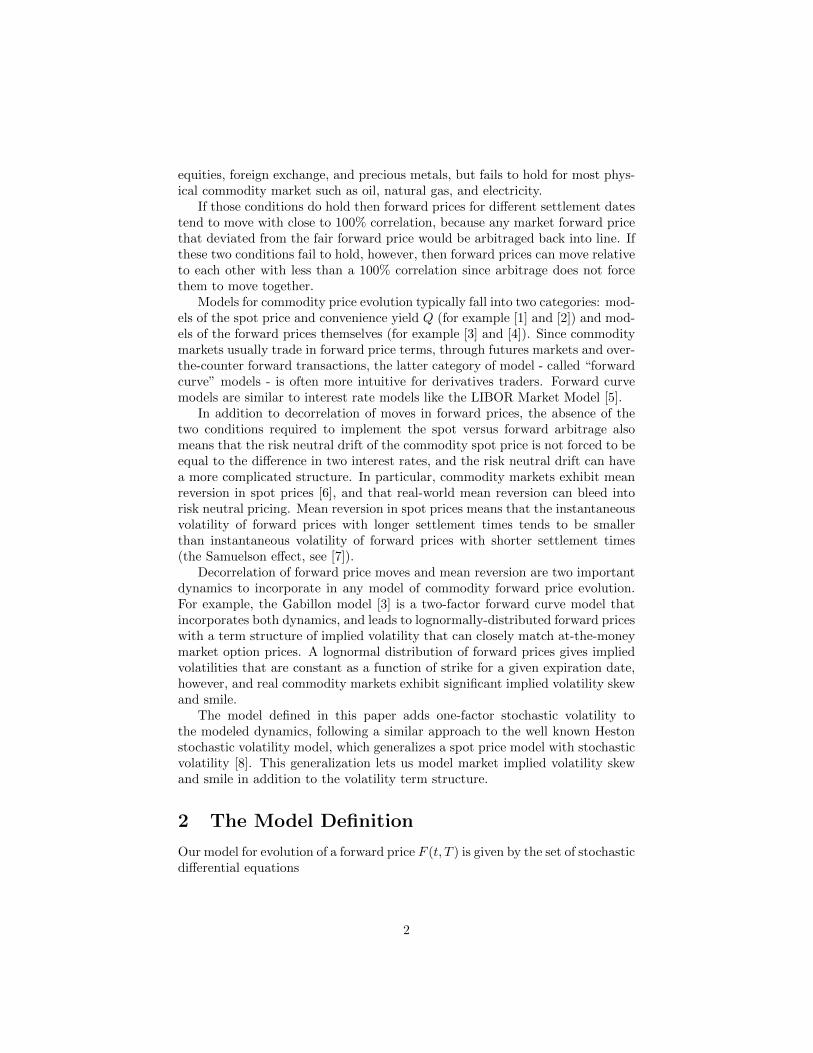
Figure 1 shows at-the-money forward implied volatility as a function of timeto expiration - the term structure of volatility - for vanilla options, where te = T .Note how the implied volatility decays with time to expiration because of theSamuelson effect, as represented in this model with the two mean reversionstrengths β1 and β2. In this example the model parameters were σ = 0.4,β1 = 0.1, β2 = 1, R = 0.5, ρ = −0.3, β = 0.5, α = 1, ρ1 = 0.3, and ρ2 = 0.3.Note that in practice α ≈ 1 is a representative scale for the value of α in manycommodity markets.

Figure 2 shows vanilla option implied volatility as a function of option strikeprice (with forward = 1) for a fixed time to expiration of te = T = 1 (otherparameters as in the previous example) which shows how the model createsimplied volatility skew.

4 Monte Carlo Simulation

Many exotic derivatives depend on more than one forward price: that is, onF (t, T ) for a range of calendar times t and settlement times T . For example,an average price option depends on daily forward price fixings during its life:one fixing for each business day (corresponding to t values), and typically forthe “prompt” futures contract (nearest to settlement on the fixing date), whichdefines the settlement times T for each fixing time t. That might mean dozensor even hundreds of separate forward curve dependencies.

In the lognormal two factor model, two separate stochastic factors can besimulated in a Monte Carlo simulation; given the values of those two factors atcalendar time t, the forward price F (t, T ) can be calculated for any value of T .This dimensionality reduction (from the full set of market values of T to thetwo stochastic factors) leads to effective numerical pricing of many derivatives.

The same is not true for this stochastic volatility extension. With x(t, T ) =

ln F (t,T )F (0,T ) ,

5

Figure 1: At-the-money forward implied volatility for vanilla options as a func-tion of expiration time. These are vanilla options so te = T . The y-axis showspercentage implied volatility and the x-axis shows time to expiration in years.

6

Figure 2: Vanilla implied volatility vs strike for a representative set of parame-ters. The y-axis shows percentage implied volatility and the x-axis shows optionstrike price (where the forward is equal to 1).

7

dx(t, T ) = −1

2v(t)σ2

F (t, T )dt+√v(t)σ

(e−β1(T−t)dz1(t) +Re−β2(T−t)dz2(t)

)(10)

If we define factors u1(t) and u2(t) as

dui(t) =√v(t)eβitdzi(t) (11)

then we can write

dx(t, T ) = −1

2v(t)σ2

F (t, T )dt+ σ(e−β1T du1(t) +Re−β2T du2(t)

)(12)

As x(0, T ) = 0 by construction we can integrate this to

x(t, T ) = −1

2

∫ t

s=0

v(s)σ2F (s, T )ds+ σ

(e−β1Tu1(t) +Re−β2Tu2(t)

)(13)

In the lognormal limit, where v(t) = 1 always, the value of x(t, T ) is specifiedonly by the two factor values u1(t) and u2(t). In the general case, however, theintegrated drift term is no longer deterministic: it depends on the path of v(t).Worse, that drift term depends on the settlement time T , so that a separatedrift term is needed for each value of T .

If the payoff being priced depends on just one value of T this is not a problem;that drift term can be calculated as an additional variable per Monte Carlo path,along with the two factors u1 and u2 and the Heston volatility factor v.

This is a computational problem for Monte Carlo simulation, however, if thederivative price depends on forwards for N � 1 values of T , because then weneed to simulate N separate drift terms on each path. For large N that canbecome computationally inefficient or too memory intensive for practical use.

We solve this problem with an approximation for the drift term. DefineI(t, T ) as

I(t, T ) =

∫ t

s=0

v(s)σ2F (s, T )ds =

∫ t

s=0

σ2F (s, T )ds+

∫ t

s=0

w(s)σ2F (s, T )ds (14)

where w(t) = v(t)− 1. The first term is deterministic, so does not suffer theproblem mentioned above. The second term, however, does suffer this problem,however, and here is where the approximation comes in: we approximate I(t, T )as

I(t, T ) ≈∫ t

s=0

σ2F (s, T )ds+ k(t, T )

∫ t

s=0

w(s)ds (15)

We choose k(t, T ) as a determinstic function such that the variance of I(t, T )under the approximation matches the true variance. If this approximation is

8

sufficiently accurate, we can run a Monte Carlo simulation and track just oneextra path variable, the integrated Heston factor

∫ ts=0

w(s)ds, and with that,the Heston volatility variable v(t) and the two regular factors u1(t) and u2(t),we can calculate any forward price F (t, T ).

If we match variances we can write

V ar(

∫ t

s=0

w(s)σ2F (s, T )ds) = V ar(k(t, T )

∫ t

s=0

w(s)ds) (16)

so that

k2(t, T ) =2∫ ts2=0

∫ s1s1=0

σ2F (s1, T )σ2

F (s2, T )E[w(s1)w(s2)]ds1ds2

2∫ ts2=0

∫ s1s1=0

E[w(s1)w(s2)](17)

To calculate this we need to calculate J(s1, s2) = E[w(s1)w(s2)] for s1 ≤ s2:

J(s1, s2) = E[w(s1)w(s2)] = E[w(s1)2] +

∫ s2

s=s1

w(s1)dw(s)

= E[w(s1)2]− β∫ s2

s1

J(s1, s)ds (18)

Then

∂J

∂s2= −βJ(s1, s2) (19)

so

J(s1, s2) = ce−β(s2−s1) (20)

for some constant c. We know that J(s1, s1) = E[w(s1)2], and from thestandard Heston model we know

E[w(t)2] =α2

2β(1− e−2βt) (21)

so

J(s1, s2) = E[w(s1)w(s2)] =α2

2β(1− e−2βs1)e−β(s2−s1) (22)

We can then evaluate the expression for this “drift factor” k(t, T ) by evalu-ating the two integrals. The resulting form is quite complex but is still closedform, and is given in appendix A.

With this expression for the drift factor we can run Monte Carlo simulationsfor pricing many derivatives by simulating the two factors u1(t) and u2(t); the

Heston volatility factor v(t); and the integrated Heston factor (∫ ts=0

w(s)ds.With that information, at any point on a Monte Carlo path, we can calculateany forward price F (t, T ).

9

5 Validating the Drift Approximation

The approximation is exact in two limits:

• Volatility of volatility is zero. In this case w(t) = v(t) − 1 is always zeroand the second term in I(t, T ) above is always zero.

• σF (t, T ) is a constant - that is, if both β1 and β2 are zero, or if β1 is zeroand R = 0.

The approximation is most extreme when there is significant volatility ofvolatility and significant term structure of σF (t, T ).

To test the size of approximation error in the case where it is expectedto be largest, we first compare the expected value of the simulated forwardbetween the factor-based Monte Carlo simulation above and an approximation-free simulation of the single forward price, using the same Monte Carlo pathsand seed to minimize the difference in simulated forwards (the difference goes tozero in the two limits above). The forward is the best metric of approximationerror since the approximation affects the risk neutral drift; if the approximationfails, the simulation will give an incorrect expected forward.

The test used parameters te = 1, T = 2, σ = 0.6, β1 = 0.01, β2 = 1, R = 0.5,ρ = −0.3, β = 0, ρ1 = 0.3, and ρ2 = 0.3. The market forward price was 1. Weused 100 time steps and 100,000 paths in the Monte Carlo simulation. Values ofα ranged from 0 to 3, which gave ATMF implied volatilities ranging from 57.4

Figure 3 shows the approximation error in basis points (one basis pointis 10−4 of the forward) for these extreme parameters as a function of α, thevolatility of volatility, running from 0 to 3. Figure 4 shows the standard erroron the simulated forward.

Note that the approximation error in the simulated forward is very small,reaching 1bp only in the most extreme market conditions where simulation erroris similarly much larger and dominates the approximation error. For example,the standard error on the forward price with 100,000 paths for α = 3 is 78bp,72 times larger than the approximation error.

The second test is for at-the-money implied volatility calculated under thetwo flavors of Monte Carlo simulation. Using the same parameters as in thefirst test, Figure 5 shows the approximation error in percentage volatility asa function of α. Figure 6 shows the standard error on the simulated impliedvolatility for the same range of α.

Again, the approximation error is very small: maximally 0.0015% in mag-nitude, versus a standard error from the simulation of around 0.14%. Theapproximation error is insignificantly small for at-the-money implied volatilitycalculations, and hence vanilla option price calculations. The implied volatilitylevel ranged from 30% to 40% across the range of α values with these parame-ters.

The final test is for out-of-the-money volatilities, where we use the sameparameters as the at-the-money volatility test but use a strike of 1.4 timesthe forward - roughly one standard deviation out-of-the-money with a one-year

10

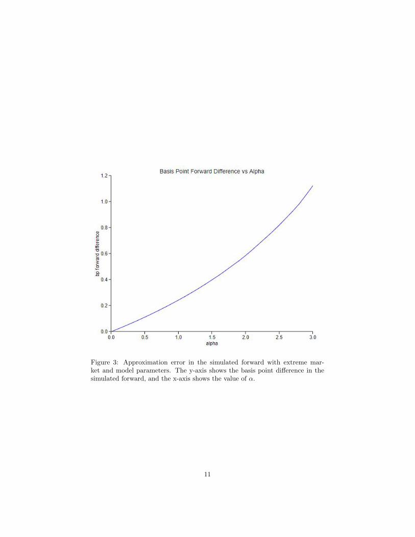
Figure 3: Approximation error in the simulated forward with extreme mar-ket and model parameters. The y-axis shows the basis point difference in thesimulated forward, and the x-axis shows the value of α.

11

Figure 4: Standard error on the expected value of the forward in the Monte Carlosimulation with extreme market and model parameters. The y-axis shows thestandard error in basis points, and the x-axis shows the value of α.

12

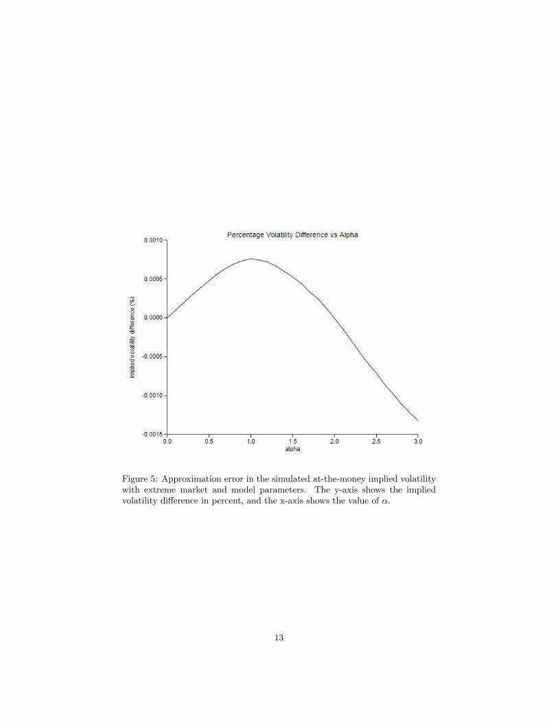
Figure 5: Approximation error in the simulated at-the-money implied volatilitywith extreme market and model parameters. The y-axis shows the impliedvolatility difference in percent, and the x-axis shows the value of α.

13

Figure 6: Standard error on the expected value of the at-the-money impliedvolatility in the Monte Carlo simulation with extreme market and model pa-rameters. The y-axis shows the standard error in percentage volatility, and thex-axis shows the value of α.

14

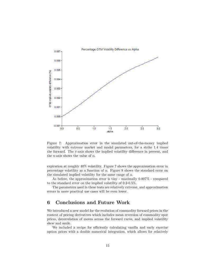
Figure 7: Approximation error in the simulated out-of-the-money impliedvolatility with extreme market and model parameters, for a strike 1.4 timesthe forward. The y-axis shows the implied volatility difference in percent, andthe x-axis shows the value of α.

expiration at roughly 40% volatility. Figure 7 shows the approximation error inpercentage volatility as a function of α. Figure 8 shows the standard error onthe simulated implied volatility for the same range of α.

As before, the approximation error is tiny - maximally 0.007% - comparedto the standard error on the implied volatility of 0.2-0.5%.

The parameters used in these tests are relatively extreme, and approximationerrors in more practical use cases will be even lower.

6 Conclusions and Future Work

We introduced a new model for the evolution of commodity forward prices in thecontext of pricing derivatives which includes mean reversion of commodity spotprices, decorrelation of moves across the forward curve, and implied volatilityskew and smile.

We included a recipe for efficiently calculating vanilla and early exerciseoption prices with a double numerical integration, which allows for relatively

15

Figure 8: Standard error on the expected value of the out-of-the-money im-plied volatility in the Monte Carlo simulation with extreme market and modelparameters, for a strike 1.4 times the forward. The y-axis shows the standarderror in percentage volatility, and the x-axis shows the value of α.

16

fast on-the-fly best fit of the model parameters to traded option prices. We alsoincluded an algorithm for pricing derivatives with a factor-based Monte Carlosimulation, under an approximation that avoids having to explicitly simulateintegrated drift factors for forwards for every settlement date included in thepayoff. The approximation error was validated as very small for practical cases.

Several areas for future work suggest themselves:

• Adding deterministic time dependency to σ. As it stands, with constantmodel parameters, the model will not be able to exactly fit at-the-moneyimplied volatility for all traded expirations. The usual approach for gettingan exact fit is to let σ be a piecewise-constant function of calendar timet or settlement time T (normally σ(t) for non-seasonal markets like crudeoil, and σ(T ) for seasonal markets like electricity and natural gas).

• Adding deterministic time dependency to α, ρ1, and/or ρ2. While con-stant values of α, β, ρ1, and ρ2 can give rise to fairly generic smile andskew term structures, it is in general not possible to calibrate the modelto reproduce market levels of implied volatility smile and skew for alltraded expiration tenors with so few parameters. Letting the parametersbe piecewise-constant functions of t or T allows for an exact calibration.

• Adding a second volatility factor. Some derivative prices are sensitiveto correlation of moves of implied volatility across different expirationtenors, and that correlation is 100% in this model because there is onlyone stochastic factor. Adding a second factor would give some controlover that volatility correlation term structure.

References

[1] Schwartz, ES The Stochastic Behavior of Commodity Prices: Implicationsfor Valuation and Hedging The Journal of Finance, Volume 52, Issue 3, July1997, Pages 923-973

[2] Hilliard, JE and Reis, J Valuation of Commodity Futures and Options underStochastic Convenience Yields, Interest Rates, and Jump Diffusions in theSpot Journal of Financial and Quantitative Analysis, Volume 33, Issue 1,March 1998, Pages 61-86

[3] Gabillon, J The term structure of oil futures prices Book: Oxford Institutefor Energy Studies, 1991

[4] Zolotko, M and Orkhrin, O Modelling the general dependence between com-modity forward curves Energy Economics, Volume 43, May 2014, Pages 284-296

[5] Rebonato, R Modern Pricing of Interest-Rate Derivatives: The LIBOR Mar-ket Model and Beyond Book: Princeton University Press, 2002

17

[6] Geman, H Mean Reversion Versus Random Walk in Oil and Natural GasPrices In: Fu MC, Jarrow, RA, Yen JYJ, Elliott RJ (eds) Advances in Math-ematical Finance. Applied and Numerical Harmonic Analysis. BirkhuserBoston, 2007

[7] Samuelson, PA Proof that properly anticipated prices fluctuate randomly In-dustrial Management Review 6 (2), 4149

[8] Heston, SL A Closed-Form Solution for Options with Stochastic Volatilitywith Applications to Bond and Currency Options The Review of FinancialStudies, Volume 6, Issue 2, 1 April 1993, Pages 327-343

A Expression for Drift Factor

The expression for the drift factor k(t, T ) used in the approximation of the riskneutral drift is a long but closed-form expression, shown here broken into piecesfor ease of display:

k2(t, T ) =2σ4β2e2βt

e2βt(2βt− 3) + 4eβt − 1(k1(T ) + k2(t, T ) + k3(t, T ) + k4(t, T ) + k5(t, T ) + k6(t, T ))

(23)with

k1(T ) = −2βe−7β1T−5β2T (k1a(T )− k1b(T ) + k1c(T )) (k1d(T )− k1e(T ) + k1f (T ))

(β − 2β1)2(β + 2β1)(β − 2β2)2(−β + β1 + β2)2(β + β1 + β2)(β + 2β2)

k1a(T ) = β2(e2(β1−β2)TR2 + 2e(β1−β2)T ρR+ 1

)k1b(T ) = β

(β2

(e2(β1−β2)TR2 + 4e(β1−β2)T ρR+ 3

)+ β1

(3e2(β1−β2)TR2 + 4e(β1−β2)T ρR+ 1

))k1c(T ) = 2

(β22 + β1

(e2(β1−β2)TR2 + 4e(β1−β2)T ρR+ 1

)β2 + β2

1e2(β1−β2)TR2

)k1d(T ) = β4

(e5β1T+3β2TR2 + 2e4(β1+β2)T ρR+ e3β1T+5β2T

)k1e(T ) = e3(β1+β2)Tβ2 (k1ea(T ) + k1eb(T ) + k1ec(T ))

k1ea(T ) = β21

(5e2β1TR2 + 8e(β1+β2)T ρR+ e2β2T

)k1eb(T ) = 2β2

(e2β1TR2 + e2β2T

)β1

k1ec(T ) = β22

(e2β1TR2 + 8e(β1+β2)T ρR+ 5e2β2T

)k1f (T ) = 4e3(β1+β2)T

(e2β1TR2β4

1 + 2β2e2β1TR2β3

1 + k1fa(T ) + 2β32e

2β2Tβ1 + β42e

2β2T)

k1fa(T ) = β21β

22

(e2β1TR2 + 8e(β1+β2)T ρR+ e2β2T

)(24)

18

k2(t, T ) =2βe−βt−7(β1+β2)T (k2a(t, T )− k2b(t, T ) + k2c(t, T )) (k2d(t, T )− k2e(t, T ) + k2f (t, T ))

(β − 2β1)2(β + 2β1)(β − 2β2)2(−β + β1 + β2)2(β + β1 + β2)(β + 2β2)

k2a(t, T ) =(e2β2t+2β1TR2 + 2e(β1+β2)(t+T )ρR+ e2β1t+2β2T

)β2

k2b(t, T ) = (k2ba(t, T ) + k2bb(t, T ))β

k2ba(t, T ) = β2

(e2β2t+2β1TR2 + 4e(β1+β2)(t+T )ρR+ 3e2β1t+2β2T

)k2bb(t, T ) = β1

(3e2β2t+2β1TR2 + 4e(β1+β2)(t+T )ρR+ e2β1t+2β2T

)k2c(t, T ) = 2

(e2β1t+2β2Tβ2

2 + β1

(e2β2t+2β1TR2 + 4e(β1+β2)(t+T )ρR+ e2β1t+2β2T

)β2 + β2

1e2β2t+2β1TR2

)k2d(t, T ) =

(e5β1T+3β2TR2 + 2e4(β1+β2)T ρR+ e3β1T+5β2T

)β4

k2e(t, T ) = e3(β1+β2)T (k2ea(t, T ) + k2eb(t, T ) + k2ec(t, T ))β2

k2ea(t, T ) =(

5e2β1TR2 + 8e(β1+β2)T ρR+ e2β2T)β21

k2eb(t, T ) = 2β1β2(e2β1TR2 + e2β2T

)k2ec(t, T ) = β2

2

(e2β1TR2 + 8e(β1+β2)T ρR+ 5e2β2T

)k2f (t, T ) = 4e3(β1+β2)T

(e2β1TR2β4

1 + 2β2e2β1TR2β3

1 + k2fa(t, T ) + 2β32e

2β2Tβ1 + β42e

2β2T)

k2fa(t, T ) = β22

(e2β1TR2 + 8e(β1+β2)T ρR+ e2β2T

)β21 (25)

k3(t, T ) =e(β2−β1)T k3a(t, T )k3b(t, T )

2(β − 2β1)2(β − 2β2)2(−β + β1 + β2)2(R2 + 2e(β2−β1)T ρR+ e2(β2−β1)T

)k3a(t, T ) = e(β1−β2)TR2 + 2ρR+ e(β2−β1)T

k3b(t, T ) = k3ba(t, T ) + k3bb(t, T ) + k3bc(t, T ) + k3bd(t, T ) + k3be(t, T )

k3ba(t, T ) = (β − 2β1)2(−β + β1 + β2)2e−4β2TR4

k3bb(t, T ) = 4(β − 2β1)2(β − 2β2)(β − β1 − β2)e−(β1+3β2)T ρR3

k3bc(t, T ) = 2(β − 2β1)(β − 2β2)e−2(β1+β2)T((2ρ2 + 1

)β2 − 2(β1 + β2)

(2ρ2 + 1

)β + β2

1 + β22 + 2β1

(4β2ρ

2 + β2))R2

k3bd(t, T ) = 4(β − 2β1)(β − 2β2)2(β − β1 − β2)e−(3β1+β2)T ρR

k3be(t, T ) = (β − 2β2)2(−β + β1 + β2)2e−4β1T (26)

19

k4(t, T ) = − e−2βt+3β1t+β2t−β1T+β2T k4a(t, T )k4b(t, T )

2(β − 2β1)2(β − 2β2)2(−β + β1 + β2)2(R2 + 2e(β1−β2)(t−T )ρR+ e2(β1−β2)(t−T )

)k4a(t, T ) = e(β1−β2)(T−t)R2 + 2ρR+ e(β1−β2)(t−T )

k4b(t, T ) = k4ba(t, T ) + k4bb(t, T ) + k4bc(t, T )k4bd(t, T ) + k4be(t, T ) + k4bf (t, T )

k4ba(t, T ) = (β − 2β1)2(−β + β1 + β2)2e−2β1t+2β2t−4β2TR4

k4bb(t, T ) = 4(β − 2β1)2(β − 2β2)(β − β1 − β2)eβ2(t−3T )−β1(t+T )ρR3

k4bc(t, T ) = 2(β − 2β1)(β − 2β2)e−2(β1+β2)T

k4bd(t, T ) = R2((

2ρ2 + 1)β2 − 2(β1 + β2)

(2ρ2 + 1

)β + β2

1 + β22 + 2β1

(4β2ρ

2 + β2))

k4be(t, T ) = 4(β − 2β1)(β − 2β2)2(β − β1 − β2)eβ1(t−3T )−β2(t+T )ρR

k4bf (t, T ) = (β − 2β2)2(−β + β1 + β2)2e2β1t−2β2t−4β1T (27)

k5(t, T ) = −k5a(t, T ) (k5b(t, T ) + k5c(t, T ) + k5d(t, T ) + k5e(t, T ) + k5f (t, T ))

k5g(t, T )k5h(t, T )

k5a(t, T ) = e(β2−β1)T(e(β1−β2)TR2 + 2ρR+ e(β2−β1)T

)k5b(t, T ) = β1(β + 2β1)(β1 + β2)(β + β1 + β2)(3β1 + β2)

k5c(t, T ) = 8β1(β + 2β1)β2(β1 + β2)(3β1 + β2)(2β + β1 + 3β2)e−(β1+3β2)T ρR3(β1 + 3β2)e−4β2TR4

k5d(t, T ) = k5da(t, T )((

2ρ2 + 1)β2 + 2(β1 + β2)

(2ρ2 + 1

)β + β2

1 + β22 + 2β1

(4β2ρ

2 + β2))R2

k5da(t, T ) = 4β1β2(3β1 + β2)(β1 + 3β2)e−2(β1+β2)T

k5e(t, T ) = 8β1β2(β1 + β2)(2β + 3β1 + β2)(β + 2β2)(β1 + 3β2)e−(3β1+β2)T ρR

k5f (t, T ) = β2(β1 + β2)(β + β1 + β2)(3β1 + β2)(β + 2β2)(β1 + 3β2)e−4β1T

k5g(t, T ) = 4β1(β + 2β1)β2(β1 + β2)(β + β1 + β2)(3β1 + β2)(β + 2β2)(β1 + 3β2)

k5h(t, T ) =(R2 + 2e(β2−β1)T ρR+ e2(β2−β1)T

)(28)

k6(t, T ) =k6a(t, T ) (k6b(t, T ) + k6c(t, T ) + k6d(t, T )k6e(t, T ) + k6f (t, T ) + k6g(t, T ))

k6h(t, T )k6i(t, T )

k6a(t, T ) = e3β1t+β2t−β1T+β2T(e(β1−β2)(T−t)R2 + 2ρR+ e(β1−β2)(t−T )

)k6b(t, T ) = β1(β + 2β1)(β1 + β2)(β + β1 + β2)(3β1 + β2)(β1 + 3β2)e−2β1t+2β2t−4β2TR4

k6c(t, T ) = 8β1(β + 2β1)β2(β1 + β2)(3β1 + β2)(2β + β1 + 3β2)eβ2(t−3T )−β1(t+T )ρR3

k6d(t, T ) = 4β1β2(3β1 + β2)(β1 + 3β2)e−2(β1+β2)T

k6e(t, T ) = R2((

2ρ2 + 1)β2 + 2(β1 + β2)

(2ρ2 + 1

)β + β2

1 + β22 + 2β1 (4β2ρ)

2+ β2

)k6f (t, T ) = 8β1β2(β1 + β2)(2β + 3β1 + β2)(β + 2β2)(β1 + 3β2)eβ1(t−3T )−β2(t+T )ρR

k6g(t, T ) = β2(β1 + β2)(β + β1 + β2)(3β1 + β2)(β + 2β2)(β1 + 3β2)e2β1t−2β2t−4β1T

k6h(t, T ) = 4β1(β + 2β1)β2(β1 + β2)(β + β1 + β2)(3β1 + β2)(β + 2β2)(β1 + 3β2)

k6i(t, T ) = R2 + 2e(β1−β2)(t−T )ρR+ e2(β1−β2)(t−T ) (29)

20