A two-dimensional design method for the hydraulic …isromac-isimet.univ-lille1.fr/upload_dir/finalpaper/117.finalpaper.pdf · A two-dimensional design method for the hydraulic turbine

A two-dimensional design method for the hydraulic turbine runner and its preliminary validation

Zbigniew Krzemianowski1*, Adam Adamkowski1, Marzena Banaszek2

ISROMAC 2016

International

Symposium on

Transport

Phenomena and

Dynamics of

Rotating Machinery

Hawaii, Honolulu

April 10-15, 2016

Abstract

The paper presents the approach to solve the inverse problem by means of a two-dimensional

axisymmetric flow model in a curvilinear coordinate system on a basis of the runner blade of the model

vertical hydraulic turbine of Kaplan type. The Vortex Lattice Method was used to obtain streamline

function that is necessary to solve the inverse problem for the designed turbine blades.

In order to solve it authors’ own numerical algorithm and code were prepared. The preliminary

verification of the prepared algorithm has been based on (1) the results of model Kaplan turbine design

obtained by means of the classical method and (2) the results of laboratory tests of the prepared

physical turbine model.

A comparison of the tested runner blade with the runner blade generated using the developed

design method indicates its large utility and applicability.

Keywords

Hydraulic machinery design — 2D model — Inverse design — Vortex Lattice Method

1 Department of Hydropower, The Szewalski Institute of Fluid Flow Machinery, Polish Academy of Sciences, Gdansk, Poland 2 Department of Energy and Industrial Apparatus, Gdansk University of Technology, Gdansk, Poland

*Corresponding author: [email protected]

INTRODUCTION

A turbomachinery designing is usually carried out by the

analysing of the existing solutions, in which flow systems

require long-time CFD analysis and then by observing the

parameters fields the shapes of blades are modified. The

verification is often related with the laboratory investigations.

Because of much less time-consuming calculations the

inverse design method (the inverse problem) has been

strongly developed. This method is much faster in obtaining

the results and has a great potential of application of the laws

governing the flow and the own procedures (e.g. concerning

the optimization).

Since many years there has been a lot of activity in the

application of the inverse problem to a turbomachinery.

A great amount of papers regarding the matter of designing

was initiated in the 80’s and 90’s until now what has been

related to the computers development. There is a huge

number of the papers concerning turbomachinery with

compressible fluids (gas and steam turbines, compressors), on

the contrary to a number of papers concerning the hydraulic

machines in which the inverse design was applied. However,

proposed through years for hydraulic machinery the inverse

design methods introduced much progress in prediction of

their performance. For instance Goto and Zangeneh [1]

presented a great usefulness of the inverse problem

application in a pump optimization. Peng et al. [2, 3] presented

interesting approach of the optimization losses and cavitation

number in the axial flow turbine runner. The common

availability of the CFD commercial codes gave possibility of an

interactive aided inverse design process of hydraulic

machines. It still remains faster less time-consuming process

than designing by analysing with the use of the CFD alone.

The interaction with the CFD allows eliminating/reducing the

secondary flows (Daneshkah and Zangeneh [4] and Zangeneh

et al. [5]) or reducing area of pressure below the vapour

pressure which means avoiding cavitation phenomenon

(Okamoto and Goto [6]). Bonaiuti et al. [7] used a blade

parameterization by means of hydrodynamic parameters like

blade loading. This approach directly influences on the

hydrodynamic flow field. Further, the CFD analysis was used to

estimate the hydrodynamic and suction performance.

Mutual interaction of the inverse problem and the CFD

calculations leads to increasing the efficiency of hydraulic

machines, but in some cases, in which fast engineering design

is required, particularly in case of the small low head hydraulic

turbines, cannot be used because of too much time required.

The essential goal of authors was to present the fast

engineering procedure of the design of the hydraulic Kaplan

turbine runner with the use of the inverse problem solution.

Proposed and developed solution is carried out in two stages.

In the first stage, a stream function was calculated based on

the Biot-Savart law utilizing the Vortex Lattice Method (VLM). It

is solved in a 2D meridional plane of turbine so the blade

thickness is not “seen” by flow and therefore is neglected. The

reason of usage of the VLM theory was to avoid assuming

streamlines a’priori. It introduces physical solution for the

streamlines. The obtained streamlines are basis for a stream

function which is required for further part of procedure in which

blade of runner is generated.

In the second stage, in order to determine the shape of the

blade runner the axisymmetric two-dimensional model is used

with the equations described in a curvilinear coordinate system

to simplify calculation. The model solves conservation equations

(mass, momentum, energy) to find two dimensional (radially and

axially) parameters distributions (in third tangential direction

Article Title — 2

parameters are circumferentially averaged). On the basis of

that it is possible to create 3D shape of blade. It is supposed

the 2D theory is more precise in flow computation than the 1D

theory because the conservation equations are more complete

in flow description.

The inverse problem presented in the paper primarily was

developed for many years at the Gdansk University of

Technology and at present has been developed at the Institute

of Fluid-Flow Machinery in Gdansk (Poland) [8, 9].

The authors verified their numerical inverse problem

method for a Kaplan turbine runner on the basis of comparison

with the geometry of model turbine runner, constructed by

means of the classical design procedure (1D theory) and

experimentally investigated at test stand. The measured

parameter distributions of that runner like: meridional and

tangential velocities and also thickness, mass flow rate,

rotational speed, head, number of blades and others were

used as the boundary conditions to calculate the new runner

blade and verify applicability of the presented procedure.

1. REFERENCE TURBINE AND ITS EXPERIMENTAL TEST

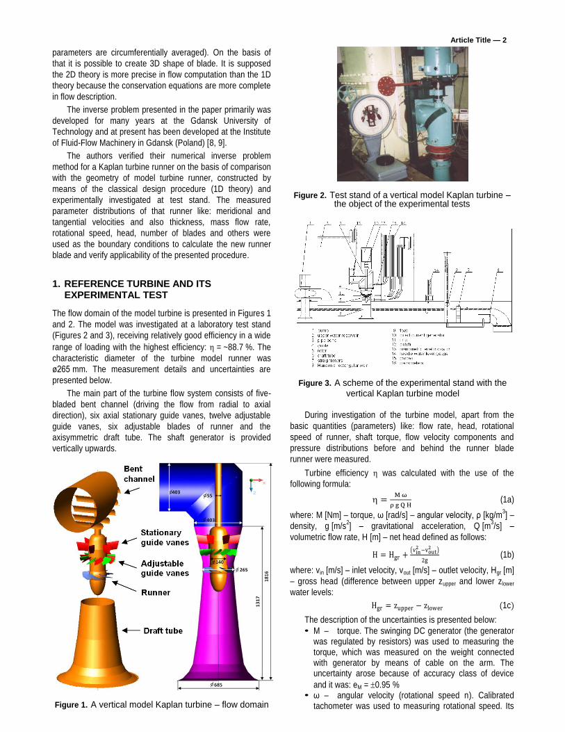
The flow domain of the model turbine is presented in Figures 1

and 2. The model was investigated at a laboratory test stand

(Figures 2 and 3), receiving relatively good efficiency in a wide

range of loading with the highest efficiency: = ~88.7 %. The

characteristic diameter of the turbine model runner was

ø265 mm. The measurement details and uncertainties are

presented below.

The main part of the turbine flow system consists of five-

bladed bent channel (driving the flow from radial to axial

direction), six axial stationary guide vanes, twelve adjustable

guide vanes, six adjustable blades of runner and the

axisymmetric draft tube. The shaft generator is provided

vertically upwards.

Figure 1. A vertical model Kaplan turbine – flow domain

Figure 2. Test stand of a vertical model Kaplan turbine – the object of the experimental tests

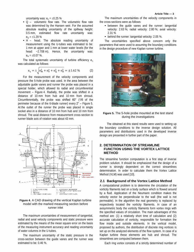
Figure 3. A scheme of the experimental stand with the vertical Kaplan turbine model

During investigation of the turbine model, apart from the

basic quantities (parameters) like: flow rate, head, rotational

speed of runner, shaft torque, flow velocity components and

pressure distributions before and behind the runner blade

runner were measured.

Turbine efficiency was calculated with the use of the

following formula:

(1a)

where: M [Nm] – torque, ω [rad/s] – angular velocity, ρ [kg/m3] –

density, g [m/s2] – gravitational acceleration, Q [m

3/s] –

volumetric flow rate, H [m] – net head defined as follows:

(1b)

where: vin [m/s] – inlet velocity, vout [m/s] – outlet velocity, Hgr [m]

– gross head (difference between upper zupper and lower zlower

water levels:

(1c)

The description of the uncertainties is presented below:

• M – torque. The swinging DC generator (the generator was regulated by resistors) was used to measuring the torque, which was measured on the weight connected with generator by means of cable on the arm. The uncertainty arose because of accuracy class of device

and it was: eM = 0.95 % • ω – angular velocity (rotational speed n). Calibrated

tachometer was used to measuring rotational speed. Its

Article Title — 3

uncertainty was: en = 0.25 % • Q – volumetric flow rate. The volumetric flow rate

was determined by the Hansen weir. For the assumed absolute reading uncertainty of the spillway height: 0.5 mm, estimated flow rate uncertainty was:

eQ = 1.29 % • H – head. The absolute reading uncertainty of

measurement using the U-tubes was estimated to be: 1 mm at upper and 1 mm at lower water levels (for the head: ~2.708 m). Hence, the uncertainty was:

eH = 0.07 %.

The total systematic uncertainty of turbine efficiency e

was calculated as follows:

(2)

For the measurement of the velocity components and

pressure the 5-hole probe was used. In the area between the

adjustable guide vanes and runner the probe was placed in a

special holder, which allowed its radial and circumferential

movement – Figure 4. Radially, the probe was shifted in a

distance of 10 mm from hub and 10 mm from shroud.

Circumferentially, the probe was shifted 60° (1/6 of the

perimeter because of the 6-blade runner) every 2° – Figure 5.

At the outlet of the runner the probe was placed in single

socket also in a distance of 10 mm from hub and 10 mm from

shroud. The axial distance from measurement cross-section to

runner blade axis of rotation was about 43 mm.

Figure 4. A CAD drawing of the vertical Kaplan turbine model with the marked measuring section before

runner inlet

The maximum uncertainties of measurement of tangential,

radial and axial velocity components and static pressure were

estimated by the means of the mean square error on the basis

of the measuring instrument accuracy and reading uncertainty

of water columns in the U-tubes.

The maximum uncertainty of the static pressure in the

cross-section between the guide vanes and the runner was

estimated to be: 0.46 %.

The maximum uncertainties of the velocity components in

the cross-sections were as follows:

• between the guide vanes and the runner: tangential velocity: 2.63 %; radial velocity: 2.80 %; axial velocity: 2.31 %

• behind the runner: tangential velocity: 2.05 %.

The uncertainties specified above concern only the

parameters that were used to assuming the boundary conditions

in the design procedure of new Kaplan runner turbine.

Figure 5. The 5-hole probe mounted at the test stand during the investigations

The obtained at this stand results were used to setting up

the boundary conditions to the inverse design solution. All

parameters and distributions used in the developed inverse

design are presented in further part of the paper.

2. DETERMINATION OF STREAMLINE FUNCTION USING THE VORTEX LATTICE METHOD

The streamline function computation is a first step of inverse

problem solution. It should be emphasized that the design of a

runner is strongly dependent on the correct streamlines

determination. In order to calculate them the Vortex Lattice

Method (VLM) was used [10].

2.1 Background of the Vortex Lattice Method

A computational problem is to determine the circulation of the

vorticity filaments laid on a body surface which is flowed around

by a fluid. Application of the Neumann condition makes the

velocity vector be perpendicular to the wall (the wall is not

permeable). In the algorithm the real geometry is replaced by

respectively located the vorticity filaments. In case of an

axisymmetric body the vorticity filaments form vortex rings with

the specified values of circulation. The main advantages of this

method are: (1) a relatively short time of calculation and (2)

accurate calculation of vorticity, responsible for formation the

flow inside and outside elements. In the vortical model,

proposed by authors, the distribution of discrete ring vortices is

set up on the analyzed elements of the flow system. In case of a

Kaplan turbine these elements are hub and shroud. The

streamlines are computed between them.

Each ring vortex consists of a strictly determined number of

Article Title — 4

vortex lines with the same equal value of circulation –

Figure 6. In the middle of the distance between two vortex

rings in the meridional surface A-A, the checkpoints K are

placed, in which boundary condition for the wall impermeability

has to be fulfilled (the Neumann condition). In general case,

meridional surface represents the meridional shape of

hydraulic turbine.

Figure 6. The scheme of the vortical mesh with the

vortex rings

Determination of a vorticity field is the primary task of the

method. Application of the Neumann condition allows for

calculation of a vortex filaments circulation. A calculated

circulation allows for the determination of the velocity field and

the distribution of streamlines in the meridional (2D) flow

channel. The following formula (3) is the discrete form of

Neumann condition written for a single checkpoint K:

(3)

where:

• s – number of a checkpoint • i – number of a ring vortex • j – number of an element (line dS) located on a

vortex ring • k – number of an axisymmetric element of a flow

channel (in this case there are two elements: hub and shroud – kmax = 2)

• Vk,i – induced velocity by vortex filament of a single vortex ring in a checkpoint K.

• V – inflow velocity in an infinity (velocity in some distance before runner)

• ns – unit normal vector to the wall at a checkpoint K • N – number of ring vortices on hub or shroud • M – number of vortex elements (lines) on a single

vortex ring.

Formula (3) is applied to each checkpoint K. This way the

linear set of equations is constituted. Velocity V is dependent

on a vortex filaments circulation. In order to calculate it the

Biot-Savart law is used to computing the velocity induced by a

vortex element [11]:

(4)

where (see Figure 6):

• – circulation of a vortex element • ds – elemental length of a vortex element • W – influence coefficient of a vortex element on

velocity in checkpoint K • R – distance between a single element and a

checkpoint K.

For a single vortex ring the coefficient of the influence W ij

can be calculated. It takes into account the influence of all

vortex ring elements (intervals). The linear set of equations in

vector notification is presented below (the influence of all

vortices on all checkpoints is taken into account):

(5)

where:

• [SM*N] – vector of values taking into account the

boundary condition (inflow velocity V in an infinity).

The result of the solution is vector of circulation values M*N.

2.2 Determination of the Streamline Function

A calculated vector of vortex ring circulation allows calculating

the components of velocity in any flow point. Assuming the axial

symmetry of the flow channel, components of velocity in the

axial Vzt and radial Vxt directions can be defined for any point t,

as follows:

(6a)

(6b)

where:

• Vx k,i – induced radial component velocity in point t by a vortex filament of single vortex ring

• Vz k,i – induced axial component velocity in point t by a vortex filament of single vortex ring

• V – inflow velocity in an infinity.

The streamline definition claims that the velocity vectors are

tangent along the whole line. Hence, having the initial point

(xt, zt) at a beginning of streamline, any further point (xt+1, zt+1)

may be calculated using the time step Δt that has to be a’priori

assumed, as follows:

(7a)

(7b)

This way the whole streamline can be calculated. To

achieve sufficiently smoothed streamline the short time step

should be assumed, otherwise local fluctuations may arise. It is

strongly recommended to carry out the numerical experiment

with different values of time steps to learn how procedure of

streamlines calculation is sensitive for it. Flow channel, due to

the proper formation of the streamline must be extended before

and after the considered flow geometry. The lengths of these

areas should be assumed so that the change of the flow

direction in runner area was not noticeable before the inlet and

Article Title — 5

behind the outlet (far inflow and far outflow should be pretty

uniform).

The inflow velocity is the one and only physical boundary

condition. In considered case, this velocity was calculated from

mass flow rate: m = 74 kg/s. Its value assumed to calculation

was: V = 0.6 m/s.

The Figure 7 shows calculated streamlines in the

considered runner. Calculations were carried out for the

following parameters:

• number of streamlines: 21 (20 intervals between hub and shroud)

• time step: t = 1e-5 s • number of elements (intervals) on hub and shroud in

axial direction: 120 + 120 • number of elements (intervals) on hub and shroud in

tangential direction (circumferential rings): 120 + 120 • number of time steps: 5000.

Presented streamlines are a basis for the mathematical

description of the streamline function, which is further used in

a 2D model for the runner blade design.

Figure 7. Meridional view of model turbine (left) and computed streamlines and mesh in flow domain of

runner (right).

Each of the 21 lines was subjected to approximation to

find its mathematical description to create streamline function

that is the radius dependent on two variables: 1) a coordinate

along the streamline (constant along it) and 2) an axial

coordinate. In the two-dimensional axisymmetric model, shown

further below, these coordinates will be respectively denoted

as follows: and . This implies denotation of a

streamline function as follows: .

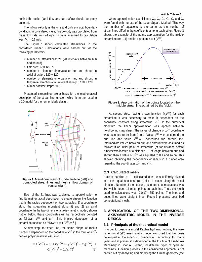
At first step, for each line, the same shape of radius

function f dependent on the coordinate in the form of a 5th-

degree polynomial was assumed:

(8)

where approximation coefficients: C1, C2, C3, C4, C5 and C6

were found with the use of the Least Square Method. This way

the number of equations is the same as the number of

streamlines differing the coefficients among each other. Figure 8

shows the example of the points approximation for the middle

streamline (no. 11) and its equation: .

Figure 8. Approximation of the points located on the middle streamline obtained by the VLM.

At second step, having known function for each

streamline it was necessary to make it dependent on the

coordinate constant along streamline: . In the numerical

algorithm the linear approxiamtion was applied between

neighboring steamlines. The range of change of coordinate

was assumed to be from 0 to 1. Value concerned the

hub line and value concerned the shroud line.

Intermediate values between hub and shroud were assumed as

follows: if an initial point of streamline (at far distance before

runner) was located at a distance 0.1 of length between hub and

shroud then a value of was equaled to 0.1 and so on. This

allowed obtaining the dependency of radius in a runner area

regarding the coordinates and .

2.3 Calculated mesh

Each streamline of 21 calculated ones was uniformly divided

into the equal sections from inlet to outlet along the axial

direction. Number of the sections assumed to computations was

16, which means 17 mesh points on each line. Thus, the mesh

used to calculations was: 21x17 = 357 points. The inlet and

outlet lines were straight lines. Figure 7 presents described

computational mesh.

3. APPLICATION OF THE TWO-DIMENSIONAL AXISYMMETRIC MODEL IN THE INVERSE DESIGN

3.1 Principals of the theoretical model

In order to design a model Kaplan hydraulic turbine, the two-

dimensional (2D) axisymmetric model was used that has been

developed at the Gdansk University of Technology for many

years and at present it is developed at the Institute of Fluid-Flow

Machinery in Gdansk (Poland) for different types of hydraulic

machines. A design process in the considered approach is not

carried out by analyzing and modifying the turbine geometry (the

Article Title — 6

direct problem), but by calculating the shape (skeleton) of the

blade directly (the inverse problem).

Two-dimensionality means that the change of parameters

takes place in a meridional plane in two directions (axial and

radial). In third direction (circumferential), the flow parameters

are averaged. The model has been derived in a special

curvilinear coordinate system. The introduction of curvilinear

coordinate system was to simplify the mathematical form of the

conservation equations: mass, momentum and energy. These

equations are transformed from the Cartesian system to the

mentioned curvilinear system described by three

coordinates: . The coordinates and were

described in the previous chapter. The third coordinate is

an angular coordinate. Presented coordinate system has two

pairs of orthogonal surfaces: and . The

third pair is non-orthogonal surface. Figure 9 shows

schematic view of a curvilinear coordinate system for a Francis

turbine.

Figure 9. Schematic view of the curvilinear

coordinate system and example of the meridional view

of a Francis runner

The introduction of the described new coordinate system

makes the velocity field be dependent on the only two

components. The third one, concerning coordinate, is

automatically equal to zero:

(9)

It should be emphasized that it is not an assumption, but

the mathematical transformation using the Christoffel Symbols

of the Second Kind, defining the transition from the Cartesian

to the curvilinear system. In other words, these are the

converters of equations from one coordinate system to

another. These symbols form a matrix of 27 coefficients (three-

dimensional matrix: 3 x 3 x 3 = 27).

The quantity U2 is an angular velocity of fluid related to

tangential velocity, denoted by , as follows:

(10a)

The quantity U3 is an axial velocity of fluid related to

meridional velocity, denoted by , as follows:

(10b)

The quantity f and the derivative mean the streamline

function (radius of runner) and its derivative:

(11)

The assumptions of the presented model are presented

below.

- axial symmetry:

- steady:

- adiabatic flow

- incompressible flow: ρ = const (in case of hydraulic

machinery – generally, compressible flow may also be

considered, e.g. in a steam turbine).

The rules of transformation between the Cartesian and

introduced curvilinear systems are listed below. It is a classic

transition between the orthogonal and cylindrical systems:

(12a)

(12b)

(12c)

3.2 Conservation equations system

The conservation equations converted from the Cartesian to the

curvilinear coordinate systems are presented below.

• Mass conservation equation (MassCE)

(13a)

where: ρ – density, – mass flow rate distribution

calculated at inlet to runner [kg/s]. The inlet surface of the

runner is reduced by material of blades, hence the above

equation contains introduced blockage coefficient .

The value of this coefficient is in the range of <0;1). Value 0

means no blades thickness. Value 1 means the total blockage of

a flow.

• Momentum conservation equation in the direction (MomCE)

(13b)

where: p – pressure, – body force potential ( , in which: g – gravitational acceleration; sign ‘+’ means that

rotational axis and gravitational force are directed in opposite

directions, while sign ‘–‘ in opposite case. Here is presented

momentum conservation equation only in direction because

it is the only used in procedure for solving the inverse problem.

• Energy conservation equation (EnerCE)

(13c)

where: ec(x(1)

) – total energy distribution calculated at inlet to

runner, – circumferential (runner) velocity, according to the

formula:

(14)

where: ω – angular velocity [rad/s], n – rotational speed

[rpm], f – radius, stream function [m].

Article Title — 7

3.3 Inverse problem solution using the characteristics method

It may be proven that presented above the partial differential

equations set is of a hyperbolic type, hence, in order to solve

the flow field inside the runner area method of characteristics

was used. This method allows converting the partial differential

equations system to an ordinary differential equation solved on

lines, which are the characteristics of the system. The

characteristics are: the streamlines (I family) and the

orthogonal lines (II family). The orthogonal lines are described

by equation as follows:

(15)

Along the orthogonal lines the following equation for

pressure can be solved:

(16)

This is the ordinary differential equation which allows

solving pressure field inside flow domain of runner. The

Figure 10, presented below, presents the shape of first and

second families of characteristics. Meridional and tangential

components of velocity are computed respectively from the

MassCE and the EnerCE.

The existence of characteristics implies the way of setting

up the boundary conditions (BC) – Figure 10. In the runner

domain three areas may be specified: I – area, in which

characteristics start at inlet of runner, II – area, in which

characteristics start at hub or shroud of runner (in presented

case – hub), III – area, in which characteristics start at outlet of

runner (if the BC is unknown at outlet then this area is covered

by characteristics starting from hub or shroud – area II).

Figure 10. I and II families of characteristics and setting

up of the boundary conditions

4. DESIGN OF THE RUNNER BLADING AND ITS EVALUATION

4.1 Boundary conditions

The distributions of parameters (velocities and pressure) in the

measurement cross-sections of turbine model and global

parameters (rotational speed and so on), assumed to

calculations, are presented below. They are obtained from

experiment at the test stand for the optimal point of work (the

highest efficiency).

The global parameters used to calculations were as follows:

• Number of blades: 6

• Meridional shape (inlet and outlet lines of runner) at blade

angle position from its closure: = 16

• Rotational speed: n = 650 rpm

• Mass flow rate: m = 74 kg/s

• Head: H = 2.725 m

• Density: = 999.1 kg/m3

• Gravitational acceleration: g = 9.81 m/s2

• Thickness assumed similar to the reference case.

The circumferentially averaged measured distributions of

tangential , meridional components of velocity and

pressure p regarding the radius were approximated by means of

the Least Square Method (LSM). The measured and

approximated lines and their equations by the LSM are

presented in the respective Figures 11, 12, 13, 14, 15.

It is worth to highlight that the meridional component of

velocity was re-calculated from the measurement cross-section

to the runner inlet cross-section for the calculated streamline

function with the use of the MassCE. The necessity of such

recalculation resulted from the changed shape of streamlines

and different areas of the mentioned cross-sections. Figure 11

shows the measured and approximated distributions of the

meridional velocity regarding the radius in the measurement

cross-section (the distribution is regarding the radius from hub

(fmin = 0) to shroud (fmax = 59 mm in case of the runner inlet or

fmax = 63 mm in case of the runner outlet). Figure 12 shows the

recalculated distribution of the meridional velocity regarding the

radius at inlet of the designed runner.

Figure 11. The measured (red) and assumed to design (black) circumferentially averaged meridional velocity in the measurement cross-section between turbine guide

vanes and runner

Figure 12. The meridional velocity assumed to design at

the runner inlet

Article Title — 8

The distributions of the other parameters: tangential

velocity and pressure were assumed to calculations without

modification. The reason of that approach was the assumption

of lack of essential impact of the distance between

measurement cross-section and designed runner inlet cross-

section – Figures 13 and 14.

Figure 13. The measured (red) and assumed to design

(black) circumferentially averaged tangential velocity in

the measurement cross-section between turbine guide

vanes and runner

Figure 14. The measured (red) and assumed to

design (black) circumferentially averaged pressure in

the measurement cross-section between turbine guide

vanes and runner

Additionally, in opposite to a common design process, in

which the tangential velocity is usually assumed to be equalled

to zero at runner outlet, in this case the measured tangential

velocity was assumed to calculation – Figure 15.

Figure 15. The measured (red) and assumed to

design (black) circumferentially averaged tangential

velocity in the measurement cross-section behind

runner

The distribution of parameters like tangential velocity

or pressure p or blade angle had to be specified at hub in

area II to start the orthogonal characteristics (see Figure 10). In

the considered case the tangential velocity regarding the axial

coordinate distribution: was assumed.

The assumed distribution, on the one hand, had to take into

account the results obtained in points located at hub line in area

I (3 points) – see Figure 16. On the other hand, it had to take

into account the similar results obtained in points located at hub

line in area III (2 points). The calculated parameters in

mentioned points imposed the shape of distribution in area II.

The 4th

-degree polynomial was taken to calculations – shown in

Figure 16.

Figure 16. Tangential velocity at the hub approximated on

a basis of computed parameters in points of area I and

area III – the boundary condition for area II 4.2 Results of the runner design

Hereafter are presented the results of the runner design.

Figure 17 shows the top and side views of the new 6-blade

Kaplan runner.

Figure 17. The top and side views of the newly designed 6-blade Kaplan runner

Article Title — 9

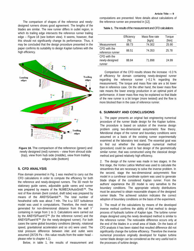
The comparison of shapes of the reference and newly-

designed runners shows good agreement. The lengths of the

blades are similar. The new runner differs in outlet region, in

which its trailing edge intersects the reference runner trailing

edge – Figure 18 (see bottom view). It seems, however, that

this should not significantly change its performance. Thus, it

may be concluded that the design procedure presented in the

paper confirms its suitability to design Kaplan turbines with the

high efficiency.

Figure 18. The comparison of the reference (green) and newly designed (red) runners – view from shroud side (top), view from hub side (middle), view from trailing

edges side (bottom)

5. CFD ANALYSIS Flow domain presented in Fig. 1 was meshed to carry out the

CFD calculations in order to compute the efficiency for both

the reference and newly-designed runners. The 3D mesh for

stationary guide vanes, adjustable guide vanes and runner

was prepared by means of the NUMECA/AutoGrid5™. The

rest of flow domain (bent conduit, draft tube) was prepared by

means of the ANSYS/Gambit™. The total number of

hexahedral cells was about 7 mln. The k-ω SST turbulence

model was used in computations. Therefore, the mesh was

generated for non-dimensional distance from the wall Y+

containing in range from 1 to 3. Calculations were carried out

by the ANSYS/Fluent12™ (for the reference runner) and the

ANSYS/Fluent16™ (for the newly-designed runner). For both

cases the same global boundary conditions (density, rotational

speed, gravitational acceleration and so on) were used. The

total pressure difference between inlet and outlet were

assumed (26726 Pa – this value results from the water head –

please refer to chapter 4.1).

Below, in table 1, the results of measurement and

computations are presented. More details about calculations of

the reference runner are presented in [12].

Table 1. The results of the measurement and CFD calculations

Efficiency

[%]

Mass flow rate

[kg/s]

Torque

[Nm]

Measurement 88.73 74.302 25.90

CFD with the

reference runner 88.51 74.353 25.78

CFD with the

newly-designed

runner

88.84 71.898 24.99

Comparison of the CFD results shows the increase ~0.3 %

of efficiency for domain containing newly-designed runner

regarding the reference runner (~0.1 % regarding the

measurement). The torque and mass flow rate are a bit lower

than in reference case. On the other hand, the lower mass flow

rate means the lower energy production in an optimal point of

performance. A lower mass flow may be explained so that blade

of the new runner is a bit longer (more twisted) and the flow is

more blocked than in the case of reference runner.

6. SUMMARY AND CONCLUSIONS

1. The paper presents an original fast engineering numerical

procedure of the runner blade design for the Kaplan turbine.

The procedure is based on solution of the inverse design

problem using two-dimensional axisymmetric flow theory.

Meridional shape of the runner and boundary conditions were

assumed on a basis of the existing runner experimentally

examined at the laboratory test stand. The essential goal was

to find out whether the developed numerical method

(procedure) could be used to fast design of the geometrically

similar runner, that was constructed using the classical design

method and gained relatively high efficiency.

2. The design of the runner was made in two stages. In the

first stage, the Vortex Lattice Method was used to calculate the

streamlines that are necessary to solve the inverse problem. In

the second, stage the two-dimensional axisymmetric flow

model in a curvilinear coordinate system was used to generate

blade shape of the considered Kaplan runner. From the

authors’ experience the 2D model is very sensitive to the

boundary conditions. The appropriate velocity distributions

must be assumed to obtain reasonable shapes of the designed

runner blade. The achieved solution indicates the correct

adoption of boundary conditions on the basis of the experiment.

3. The result of the calculations by means of the developed

inverse method confirms the ability of that method to design

process of hydraulic turbine of Kaplan type. The turbine runner

shape designed using the newly developed method is similar to

the reference runner. The noticeable difference occurs only at

the end of the blades in a small area of blade. On the basis of

CFD analysis it has been stated that resulted difference did not

significantly change the turbine efficiency. Therefore the inverse

numerical procedure originally developed for Kaplan turbine

runner blade design can be considered as the very useful tool in

the processes of turbine design.

Article Title — 10

REFERENCES

[1] A. Goto and M. Zangeneh. Hydrodynamic design of pump

diffuser using inverse design method and CFD. J. of Fluids

Engineering, 124(2), June 2002. [2]

G. Peng, S. Cao, M. Ishizuka and S. Hayama. Design

optimization of axial flow hydraulic turbine runner: Part I –

an improved Q3D inverse method. Int. J. for Numerical

Methods in Fluids, 39:517–531, 2002. [3]

G. Peng, S. Cao, M. Ishizuka and S. Hayama. Design

optimization of axial flow hydraulic turbine runner: Part II –

multi-object constrained optimization method. Int. J. for

Numerical Methods in Fluids, 39:533–548, 2002. [4]

K. Daneshkah and M. Zangeneh. Parametric design of a

Francis turbine runner by means of a three-dimensional

inverse design method. IOP Conf. Series: Earth and

Environmental Science, 12, 012058, 2010. [5]

M. Zangeneh, A. Goto and T. Takemura. Suppression of

secondary flows in a mixed flow pump impeller by

application of 3D inverse design method: Part 1-Design

and numerical validation. Transactions ASME Journal of

Turbomachinery, 118:536–543, 1996. [6]

H. Okamoto and A. Goto. Suppression of cavitation in a

Francis turbine runner by application of 3D inverse design

method. ASME Joint U.S.-European Fluids Engineering

Division Conference, paper no. 31192:851-858, 2002. [7]

D. Bonaiuti, M. Zangeneh, R. Aartojarvi and J. Eriksson.

Parametric design of a waterjet pump by means of inverse

design. CFD calculations and experimental analyses.

J. of Fluids Engineering, 132(3), 031104, Mar 18, 2010. [8]

R. Puzyrewski and Z. Krzemianowski. 2D model of guide

vane for low head hydraulic turbine. Analytical and

numerical solution of inverse problem. J. of Mechanics

Engineering and Automation, Vol. 4, No. 3:195-202, ISSN

2159-5275 (Print), ISSN 2159-5283 (Online), 2014. [9]

R. Puzyrewski and Z. Krzemianowski. Two concepts of

guide vane profile design for a low head hydraulic turbine.

J. of Mechanics Engineering and Automation, Vol. 5,

No. 4:201209. ISSN 2159-5275 (Print), 2159-5283

(Online), 2015. [10]

R. I. Lewis. Vortex Element Methods for fluid dynamics

analysis of engineering systems. Cambridge University

Press, 1991. [11]

A. Góralczyk, P. Chaja and A. Adamkowski. Method for

calculating performance characteristics of hydrokinetic

turbines. TASK Quarterly 15, No. 1:43-47, Gdansk,

Poland, ISSN 1428-6394, 2011. [12]

Z. Krzemianowski, M. Banaszek and K. Tesch.

Experimental validation of numerical model within a flow

configuration of the model Kaplan turbine. Mechanics and

Mechanical Engineering. International Journal. Volume 15,

No. 3, Lodz University of Technology Publishing, Lodz,

Poland. ISSN 1428-1511, 2011.