A trace formula for the nodal count sequence

Eur. Phys. J. Special Topics 145, 217–229 (2007)c© EDP Sciences, Springer-Verlag 2007DOI: 10.1140/epjst/e2007-00158-y

THE EUROPEANPHYSICAL JOURNALSPECIAL TOPICS

A trace formula for the nodal count sequence

Towards counting the shape of separable drums

S. Gnutzmann1,2,3,a, P. Karageorge4,b, and U. Smilansky1,4,c

1 Department of Physics of Complex Systems, The Weizmann Institute of Science,Rehovot 76100, Israel

2 Fachbereich Physik, Freie Universitat Berlin, Arnimallee 14, 14195 Berlin, Germany3 School of Mathematical Sciences, University of Nottingham, Nottingham NG7 2RD, UK4 School of Mathematics, Bristol University, Bristol BS8 1TW, UK

Abstract. The sequence of nodal count is considered for separable drums. Arecently derived trace formula for this sequence stores geometrical informationof the drum. This statement is demonstrated in detail for the Laplace-Beltramioperator on simple tori and surfaces of revolution. The trace formula expresses thecumulative sum of nodal counts This sequence is expressed as a sum of two parts:a smooth (Weyl like) part which depends on global geometrical parameters, and afluctuating part which involves the classical periodic orbits on the torus and theiractions (lengths). The geometrical context of the nodal sequence is thus explicitlyrevealed.

1 Introduction

More than 200 years ago, when Ernst Florens Friedrich Chladni found the sound figures whichnow bear his name, he tried to classify the emerging patterns e.g. by the number of lines orthe number of domains defined by the lines [1]. We are happy to dedicate a piece of work toE.F.F. Chladni whose 250th birthday we celebrate this year which follows his ideas closely.Chladni’s work inspired research in physics and in mathematics until today. He not only con-siderably advanced the knowledge on resonance and wave phenomena but also introduced thenodal set as a new concept in the research of wave phenomena which is visualised in the soundfigures. The nodal set is the zero set of a wave function. In the two dimensional case of vibratingplates or drums the nodal set consists of nodal lines which are the borders of nodal domains,i.e. maximally connected domains where the sign of the wave function does not change.We consider drums (or quantum billiards) as the eigenproblem

−∆Mψ(x) = Eψ(x) (1)

of the Laplace-Beltrami operator −∆M on a compact Riemann surfaceM (ifM has a boundarywe consider Dirichlet boundary conditions on ∂M). The spectrum En∞n=1 is discrete and canbe ordered En ≤ En+1. The eigenfunction ψn corresponding to the eigenvalue En can becharacterized by the number νn of its nodal domains. The intimate connection between thespectra, wave equations, and nodal sets is well known and frequently used or investigated invarious branches of physics and mathematics (see [2] for a recent review). The relation between

a e-mail: [email protected] e-mail: [email protected] e-mail: [email protected]

218 The European Physical Journal Special Topics

the nodal count and the spectrum is highlighted by Sturm’s oscillation theorem [3] that statesthat in one dimension the n-th eigenfunction has exactly n nodal domains. In higher dimensionsCourant proved that the number of nodal domains νn of the n-th eigenfunction cannot exceedn [3]. More recently, statistical properties of the nodal count have been investigated. It wasshown that the fluctuations in the nodal count sequence νn∞n=1 display universal featureswhich distinguish clearly between integrable (separable) and chaotic systems [4]. This statisticalapproach also lead to surprising connections with percolation theory [5] and the Schramm-Loewner evolution [6,7].Numerical and analytical evidence lead to the belief that the sequence of nodal counts in a

billiard contains a lot of information about the dynamics and the geometry, beyond thedifference between integrable and chaotic. This lead to the question [8,9]: ‘Can one countthe shape of a drum?’ This is a reformulation of the famous question by Kac [10]: ‘Can onehear the shape of a drum?’ More precisely, the question is: does the sequence of nodal countsdetermine the geometry of a drum (compact Riemmannian surface)? The independence ofthe inverse counting question from Kac’ question has been shown in that nodal counting candistinguish between some isospectral systems [8,11]. For separable systems a trace formula forthe nodal counting sequence has been established that explicitly shows the dependence of thenodal sequence on the geometry of the surface in both the smooth (Weyl-like) and the fluctu-ating parts. Thus, the nodal count trace formula is similar in structure to the correspondingspectral trace formula [12–15]. The sequence of nodal counts does not involve any spectralinformation (apart from the order) yet the nodal count trace formula contains all informationon periodic orbits on e.g. surfaces of revolution. Thus it is an important step towards ‘counting’the shape of such surfaces.In this paper we give a more detailed account of the nodal count trace formulae for convex

smooth surfaces of revolution and for simple two-dimensional tori. Generalizations to otherRiemannian manifolds in two or more dimensions are possible, provided the wave equation isseparable.

2 The cumulative nodal count

If the spectrum of the Laplace-Beltrami operator on a compact Riemannian manifold is void ofdegeneracies we may order the spectrum such that En < En+1. The corresponding nodal countsνn then form an ordered sequence which will be central to this discussion. Let [[K]] denote thelargest integer smaller than K ∈ R, then we define the cumulative nodal count

C(K) =

[[K]]∑n=1

νn for K > 0. (2)

To generalize this definition to degenerate spectra one has to uniquely choose a basis ofwave functions in the degeneracy eigenspace and also decide on the order in which they appearin the nodal counting sequence. There are several more or less natural ways to do this. Forseparable systems which are the focus of this paper we propose to choose the unique (real)basis in which the wave functions appear in product form. This still does not suffice to set aunique order within the degenerate states. Chosing an unambiguous order can be circumventedby modifying the definition of the cumulative nodal count in the following way. First define thefunction

c(E) =

∞∑n=1

νnΘ(E − En) (3)

which is independent of the order of the nodal counts. Here, Θ(x) is Heaviside’s step function.This comes at the price that now the function is based on information obtained from both thenodal counting sequence and the exact positions of the eigenvalues. To eliminate the dependence

Nodel Patterns in Physics and Mathematics 219

on the latter, we use the ε-smoothed spectral counting function

Nε(E) =∞∑n=1

Θε(E − En), (4)

where Θε(x) is a continuous, symmetric and monotonically increasing function with

limε→0Θε(x) = Θ(x).

As a consequence, for finite ε, Nε(E) is a continuous strictly monotonically increasing func-tion which can be inverted. Let Eε(K) as the solution of Nε(E) = K. Then we define themodified cumulative nodal count by

c(K) = limε→0 c(Eε(K)). (5)

For non-degenerate systems this is equivalent to the original definition (2) up to a trivialshift c(K) = C

(K + 12

). In the limit ε→ 0 the contribution of a g-times degenerate eigenvalue

En = En+1 = · · · = En+g−1 reduces to a single step Θ(K − (n − 1 + g

2 ))∑g

s=1 νn+s−1 atthe central index K =

(n− 1 + g2

)where the cumulative nodal count increases by the sum of

the nodal counts within the degeneracy class. We will derive a trace formula for this modifiedcumulative nodal count (omitting ‘modified’ in the sequel).

3 A trace formulae for the cumulative nodal count

Trace formulae for spectral functions like the spectral counting functionN (E) have been derivedfor many classes of drums (and more general quantum systems) and they have been appliedwith great success. In the case of separable drums, we will show that the same methods thatare used for spectral functions can be applied to spectral nodal counting function c(E) whicheventually leads to a trace formulae for c(K).The main ingredients of the derivation of spectral trace formulae for spectral functions are

the Poisson summation formula (for finite sums)

n1∑n=n0

f(n) =∞∑

N=−∞

∫ n1n0

f(n)e2πiNn dn+1

2[f(n0) + f(n1)]

=

∞∑N=−∞

∫ n1+1n0−1

f(n)e2πiNn dn− 12[f(n0) + f(n1)] (6)

and saddle point approximations to the resulting integrals.

3.1 Simple tori

Let us start with the simpler case of a 2-dim torus represented as a rectangle with side lengthsa and b and periodic boundary conditions ψ(0, y) = ψ(a, y) and ψ(x, 0) = ψ(x, b). This leadsto (real) eigenfunctions

ψn,m(x, y) =cossin

(2πn

a

)cossin

(2πm

b

)(7)

for m,n ∈ Z (cosines apply for m,n ≥ 0 and sines for negative m,n). The correspondingeigenvalues take the values

En,m = (2π)2

[n2

a2+m2

b2

]. (8)


Due to the checkerboard like structure of the nodal set, it is straight forward to count thenodal domains in the wavefunction ψn,m which gives

νm,n = (2|n|+ δn,0)(2|m|+ δm,0) . (9)

The only free parameter of the nodal count sequence for tori is the aspect ratio τ = a/bbecause the number of nodal domains is invariant to rescaling of the lengths.Applying Poisson’s summation formula (6) to the spectral counting function

N (E) =∞∑

n,m=−∞Θ(E −En,m) (10)

=∞∑

N,M=−∞

∫ ∞−∞

dn

∫ ∞−∞

dm Θ

(E − (2π)2

[n2

a2+m2

b2

])e2πi(nN+mM) (11)

all appearing integrals can be performed exactly. Here we are only interested in the leadingasymptotic behaviour obtained by saddle-point approximation of all oscillatory integrals whichgives

N (E) = AE +√8

πAE 1

4

∑r

sin(Lr√E − π4 )

L32r

+O(E− 34 ) (12)

The leading smooth term AE is obtained from the term N =M = 0 in (11) and A = ab/(4π)is proportional to the area of the torus. The sum in 12 runs over r = (N,M) ∈ Z2\(0, 0) (inthe sequel every sum over r will not include (0, 0) unless stated otherwise). These terms are

oscillatory functions of E. Here, Lr =√(Na)2 + (Mb)2 is the length of a periodic geodesic

(periodic orbit) with winding numbers r = (N,M).One can treat c(E) analogously. Here a closed analytic expression for the integrals would be

out of reach, but higher order corrections to the leading result can be obtained systematically.The leading asymptotic contributions are given by

c(E) = 2A2π2E2 + E

542112 A3π12

∑r

|MN |L72r

sin(Lr√E − π

4

)+O(E). (13)

We now have the leading asymptotic expressions for both c(E) and N (E). The next stepwould be to invert N (E) = K and eliminate the dependence of c(E) on the spectrum. However,the leading orders of the trace formula (12) for the spectral counting functions do not definea manifestly monotonically increasing function. Still, one may think of the exact inverse E(K)as an asymptotic series itself. The leading orders of this series can formally be obtained fromthe trace formula (12)

E(K) =K

A −K14232

Aπ 12∑r

sin(lr√K − π4 )l32r

+O(K0). (14)

Here, lr = Lr/√A is the re-scaled (dimensionless) length of a periodic orbit. The above step

definitely needs a more detailed justification. Here, we can only refer to the numerical teststhat we will give below.We may now replace E by E(K) in (13) to obtain the leading orders of the cumulative

nodal count c(K) ≡ c(E(K)). The latter can be written asc(K) = c(K) + cosc(K) (15)

with a smooth part

c(K) =2

π2K2 +O(K) (16)


and an oscillatory part

cosc(K) = K54

∑r

ar sin(lr√K − π

4) +O(K), (17)

where we introduced the amplitudes

ar =272

π52 l32r

(4π2|NM |

l2r− 1). (18)

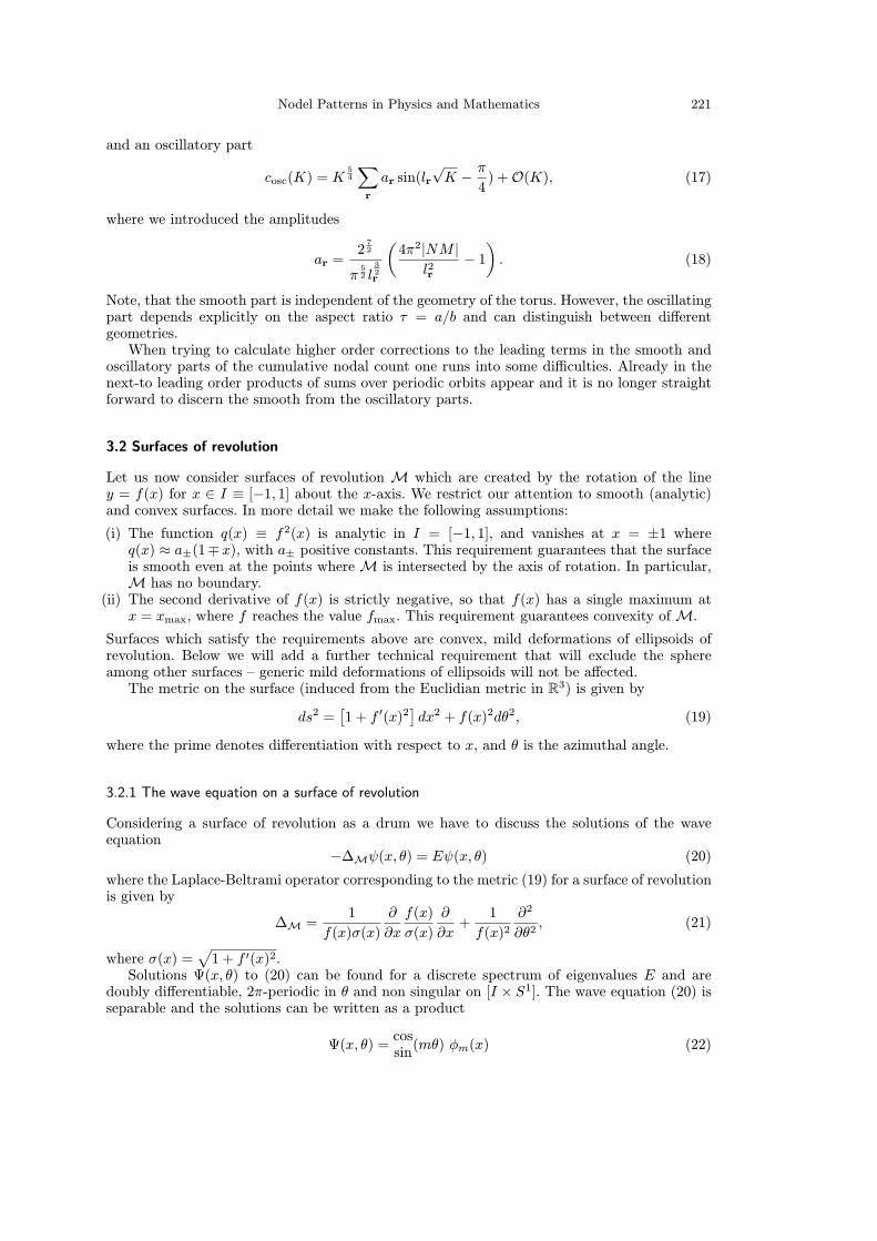
Note, that the smooth part is independent of the geometry of the torus. However, the oscillatingpart depends explicitly on the aspect ratio τ = a/b and can distinguish between differentgeometries.When trying to calculate higher order corrections to the leading terms in the smooth and

oscillatory parts of the cumulative nodal count one runs into some difficulties. Already in thenext-to leading order products of sums over periodic orbits appear and it is no longer straightforward to discern the smooth from the oscillatory parts.

3.2 Surfaces of revolution

Let us now consider surfaces of revolution M which are created by the rotation of the liney = f(x) for x ∈ I ≡ [−1, 1] about the x-axis. We restrict our attention to smooth (analytic)and convex surfaces. In more detail we make the following assumptions:

(i) The function q(x) ≡ f2(x) is analytic in I = [−1, 1], and vanishes at x = ±1 whereq(x) ≈ a±(1∓ x), with a± positive constants. This requirement guarantees that the surfaceis smooth even at the points whereM is intersected by the axis of rotation. In particular,M has no boundary.

(ii) The second derivative of f(x) is strictly negative, so that f(x) has a single maximum atx = xmax, where f reaches the value fmax. This requirement guarantees convexity ofM.

Surfaces which satisfy the requirements above are convex, mild deformations of ellipsoids ofrevolution. Below we will add a further technical requirement that will exclude the sphereamong other surfaces – generic mild deformations of ellipsoids will not be affected.The metric on the surface (induced from the Euclidian metric in R3) is given by

ds2 =[1 + f ′(x)2

]dx2 + f(x)2dθ2, (19)

where the prime denotes differentiation with respect to x, and θ is the azimuthal angle.

3.2.1 The wave equation on a surface of revolution

Considering a surface of revolution as a drum we have to discuss the solutions of the waveequation

−∆Mψ(x, θ) = Eψ(x, θ) (20)

where the Laplace-Beltrami operator corresponding to the metric (19) for a surface of revolutionis given by

∆M =1

f(x)σ(x)

∂

∂x

f(x)

σ(x)

∂

∂x+

1

f(x)2∂2

∂θ2, (21)

where σ(x) =√1 + f ′(x)2.

Solutions Ψ(x, θ) to (20) can be found for a discrete spectrum of eigenvalues E and aredoubly differentiable, 2π-periodic in θ and non singular on [I × S1]. The wave equation (20) isseparable and the solutions can be written as a product

Ψ(x, θ) =cossin(mθ) φm(x) (22)


where m ∈ Z to ensure 2π-periodicity in θ. In the seperation ansatz (22) we choose to use thecosine for m ≥ 0 and the sine for m < 0.For any fixed m, (21) now reduces to the ordinary differential equation

− 1

f(x)σ(x)

d

dx

f(x)

σ(x)

d

dxφm(x) +

m2

f(x)2φm(x) = Eφm(x) (23)

which is of the Sturm-Liouville type. Let us denote the eigenvalues En,m and eigenfunctionsφn,m(x), where n = 0, 1, 2, . . . and En,m ≤ En+1,m. Sturm’s oscillation theorem then impliesthat φn,m(x) has n nodes.The nodal pattern of the wave ψn,m(x, θ) = φn,m(x)

cossin (mθ) is that of a checkerboard typical

to separable systems and contains

νn,m = (n+ 1)(2|m|+ δm,0) (24)

nodal domains.

3.2.2 The semiclassical approach to the spectrum

To proceed further we also need to know the eigenvalues En,m. For n,m 1 the latter can bereplaced by the semiclassical eigenvalues using the Bohr-Sommerfeld approximation [13]

Escln,m =H

(n+1

2,m

)+ h(n,m) , n ∈ N, m ∈ Z . (25)

whereH(n,m) is the classical Hamiltonian defined in terms of the action variables, and h(n,m)is homogeneous of order 0. Neglecting h(n,m) in the sequel, amounts to introducing an errorwhich is bounded by a constant. As indicated by the notation the action variables m and nin (25) coincide with the integers m and n used in the separation ansatz above. Note, that ingeneral classical integrability leads to analogous semiclassical approximations for the spectrum.However classical integrability does not imply quantum separability. In our approach we usethe property of quantum separable drums that the nodal sets have a checkerboard structurewhich implies that the number of nodal domains is an explicit function νn,m = ν(n,m) of theaction variables n and m (basically a product). Since quantum separability implies classicalintegrability our approach can be generalized to all drums for which the wave equation isseparable.The classical Hamiltonian H(n,m) can be obtained from the observation that the classical

trajectories are the geodesics on the surface. The latter can be derived from the Euler-Lagrangevariational principle with the Lagrangian

L ≡ v2

4=1

4

([1 + f ′(x)2

]x2 + f(x)2θ2

). (26)

where a dot above denotes time derivative (the factor 1/4 in front of the squared velocity isconsistent with our choice of energy and action units). The angular momentum along the axis

pθ = f(x)2θ/2 is conserved and we shall use it as the first action variablem = 1

2π

∫ 2π0

pθdθ ≡ pθ.The momentum conjugate to x is

px =1

2

[1 + f ′(x)2

]x, (27)

and the conserved kinetic energy is obtained by a Legendre transformation

E ≡H(px, x,m) = pθ θ + pxx−L = p2x1 + f ′(x)2

+m2

f(x)2(28)


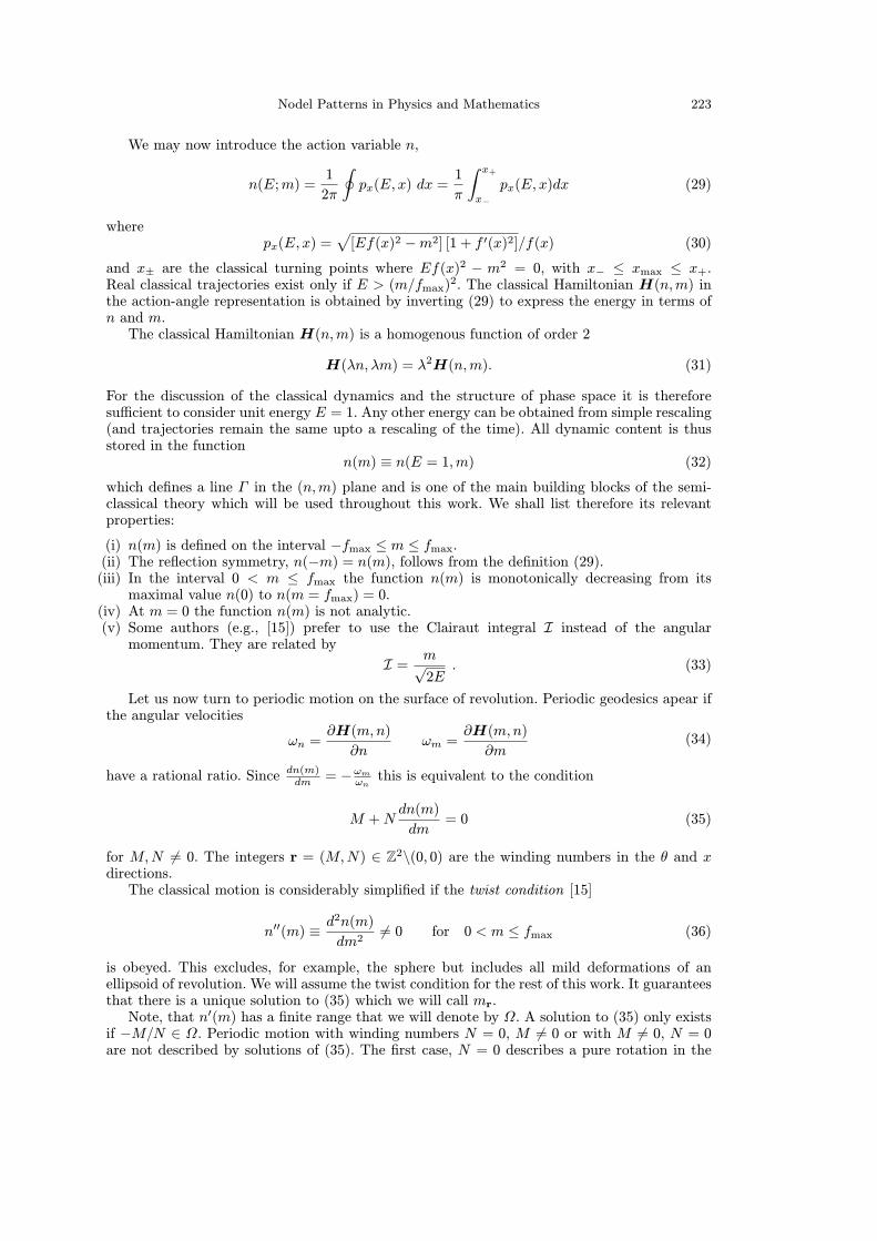
We may now introduce the action variable n,

n(E;m) =1

2π

∮px(E, x) dx =

1

π

∫ x+x−

px(E, x)dx (29)

wherepx(E, x) =

√[Ef(x)2 −m2] [1 + f ′(x)2]/f(x) (30)

and x± are the classical turning points where Ef(x)2 − m2 = 0, with x− ≤ xmax ≤ x+.Real classical trajectories exist only if E > (m/fmax)

2. The classical Hamiltonian H(n,m) inthe action-angle representation is obtained by inverting (29) to express the energy in terms ofn and m.The classical Hamiltonian H(n,m) is a homogenous function of order 2

H(λn, λm) = λ2H(n,m). (31)

For the discussion of the classical dynamics and the structure of phase space it is thereforesufficient to consider unit energy E = 1. Any other energy can be obtained from simple rescaling(and trajectories remain the same upto a rescaling of the time). All dynamic content is thusstored in the function

n(m) ≡ n(E = 1,m) (32)

which defines a line Γ in the (n,m) plane and is one of the main building blocks of the semi-classical theory which will be used throughout this work. We shall list therefore its relevantproperties:

(i) n(m) is defined on the interval −fmax ≤ m ≤ fmax.(ii) The reflection symmetry, n(−m) = n(m), follows from the definition (29).(iii) In the interval 0 < m ≤ fmax the function n(m) is monotonically decreasing from its

maximal value n(0) to n(m = fmax) = 0.(iv) At m = 0 the function n(m) is not analytic.(v) Some authors (e.g., [15]) prefer to use the Clairaut integral I instead of the angularmomentum. They are related by

I = m√2E

. (33)

Let us now turn to periodic motion on the surface of revolution. Periodic geodesics apear ifthe angular velocities

ωn =∂H(m,n)

∂nωm =

∂H(m,n)

∂m(34)

have a rational ratio. Since dn(m)dm

= −ωmωnthis is equivalent to the condition

M +Ndn(m)

dm= 0 (35)

for M,N = 0. The integers r = (M,N) ∈ Z2\(0, 0) are the winding numbers in the θ and xdirections.The classical motion is considerably simplified if the twist condition [15]

n′′(m) ≡ d2n(m)

dm2= 0 for 0 < m ≤ fmax (36)

is obeyed. This excludes, for example, the sphere but includes all mild deformations of anellipsoid of revolution. We will assume the twist condition for the rest of this work. It guaranteesthat there is a unique solution to (35) which we will call mr.Note, that n′(m) has a finite range that we will denote by Ω. A solution to (35) only exists

if −M/N ∈ Ω. Periodic motion with winding numbers N = 0, M = 0 or with M = 0, N = 0are not described by solutions of (35). The first case, N = 0 describes a pure rotation in the


θ-direction at constant x = xmax where m0,±|M | = ±fmax and the second case M = 0 is aperiodic motion through the two poles at fixed angle θ mod π such that m|N |,0 = 0.The length of a periodic geodesic can be obtained by observing that E = v2/4 is a constant

of motion the metric length L =∮v2dt/v of a periodic geodesic is given by

Lr = 2π |Nn(mr) +Mmr| . (37)

Returning to the spectrum, we note that the leading terms in the trace formula for the spectralcounting function N(E) =

∑m,nΘ(E − En,m) can be obtained by using (25) and Poisson’s

summation formula [15].

N (E) = AE + E 14

∑r

Nr(E) (38)

where

A =∫ fmax−fmax

n(m) dm = ||M||/4π (39)

and ‖M‖ is the area of the surface. The oscillating parts contain integrals

Nr ∝∫ fmax−fmax

dm e2πi√E[Nn(m)+Mm]. (40)

We will calculate these to leading order in E12 using the stationary phase approximation.

The stationary phase condition turns out to be identical to equation (35) which describesperiodic motion. As a consequence the stationary points are m = mr. Note that the rangeof contributing r values is restricted to the classically accessible domain −M/N ∈ Ω. For−M/N /∈ Ω the integral does not have a stationary point and contributes only to higher ordersin 1/

√E. Eventually one obtains, in stationary phase approximation [15]

Nr(E) = (−1)N sin(LrE12 + σ π4 )

2π|N3n′′r | 12+O(E− 12 ) (41)

where n′′r = n′′(m = mr) and σ = sign(n′′r ) which is the same for all values of r. The contribu-tions of the terms with either N = 0 or M = 0 or with −M/N /∈ Ω are of higher order in 1/Eand will not be considered here.

3.2.3 The cumulative nodal count

We have now all ingredients to derive an asymptotic trace formula for the cumulative nodalcount

c(K) = c(E(K)) =

∞∑n=0

∞∑m=−∞

νmn Θ(E(K)− Em,n) . (42)

Inverting the asymptotic trace formula (38) for the spectral counting function N (E) = Kone obtains

E(K) =K

A −(K

A) 14∑r

Nr(KA )A +O(K0) (43)

to leading order in 1/K.The function c(E) can be obtained as an asymptotic trace formula by the same approach

that we used forN (E) in the preceding section 3.2.2. Expanding the result in δE = E(K)−K/Asuch that

c(K) = c(K/A) + c′(K/A)δE +O(c′′δE2) (44)


is consistent if we neglect all orders smaller than O(K). In almost complete analogy to thetrace formula (15) for simple tori, this can be expressed as a sum

c(K) = c(K) + cosc(K) (45)

of a smooth part c(K) and an oscillatory part, cosc(K). Defining

mpnq =1

A∫E(m,n)<1

dm dn |m|pnq (46)

as the action moments (averaged over the area under the curve Γ ) the smooth part can beexpressed as

c(K) = 2mn

A K2 +m

A 12

K32 +O(K) (47)

which, compared to the trace formula of the torus (15), has an additional term ∝ K3/2 whichcan be traced back to the different way of counting nodal domains in tori (9) and surfaces ofrevolution (24). Likewise, the oscillatory part can be expressed as

cosc(K) = K54

∑r:−MN ∈Ω

ar sin(lr√K +

σπ

4

)+O(K) (48)

with the amplitude

ar = (−1)Nmrn(mr)− 2mnA 54π|N3n′′r | 12

(49)

and rescaled length

lr =Lr√A (50)

of a periodic geodesic r with −MN∈ Ω. Note, that for mr = 0 or mr = ±fmax only one half of

the stationary phase integral contributes and the amplitude ar has to be multiplied by 1/2. Ifthe (finite) interval Ω ⊂ R is bounded by rational numbers, then the amplitudes ar for periodicgeodesics with winding numbers satisfying −M

N∈ ∂Ω also have to be multiplied by 1/2.

The above trace formula reveals a quite astonishing relation between the nodal countsequence and the geometry of the surface. So far, similar relations have only beenderived for spectral functions. Yet the cumulative nodal count does not contain any spectralinformation apart from the ordering inherited from the spectrum and still the oscillatory partcan be written as a sum over all different periodic geodesics.For ellipsoids defined by the rotation of the curve

f(x) = R√1− x2 (51)

with maximal radius fmax = R at the equator the curve n(m) can be expressed explicitly interms of elliptic integrals.

4 Application of the trace formula and comparison to numerical results

We have tested the approximations in the above calculations numerically on four differentsystems for which we built up a large data base which will be denoted as data sets (a) to (d).We chose two different ellipsoids of revolution with R = 2 (for data set (a)) and R = 1/2 (fordata set (b)). These parameters provide us with data sets for an oblate (R = 2) and prolate(R = 1/2) ellipsoid. We also considered two different tori with τ2 = 2 (for data set (c)) and

τ2 =√2 (for data set (d)). For rational τ2 the spectrum contains growing number theoretic

degeneracies which are absent in the irrational case. Our parameters cover both cases.


102 104 106

105

1010

1015

1020

a)

b)

c)

d)

K

R (K )

Fig. 1. The integrated variance R(K) (double logarithmic plot, the plots have been shifted for bettervisibility) for the two ellipsoids (data set (a) with R = 2 and data set (b) with R = 1/2), and the twotori (data set (c) with τ2 = 2 and data set (d) with τ2 =

√2). The full line has slope 7/2.

For the ellipsoids the first 105 eigenvalues and eigenfunctions have been calculated, fromwhich we constructed the sequence of nodal counts. For the tori obtaining the spectrum and thecorresponding eigenfunctions is straight forward – in our numerics we used the lowest ≈ 4×106eigenvalues.To obtain the fluctuating part the numerically computed c(K) were fitted to a fourth order

polynomial in κ =√K. Not surprisingly, the numerically obtained two leading coefficients

(∝ K2 and K3/2) fitted extremely well with the corresponding analytically obtained coefficientsin the smooth parts of the corresponding trace formulae.The more critical tests, which we will present here, involve the fluctuations decribed by the

oscillatory part of the trace formulae. The latter has been obtained numerically by subtractingthe best polynomial fit from the exact c(K).The tests of on the oscillatory part of the trace formulae give us also the opportunity to

discuss some aspects of the fluctuations of the cumulative nodal count sequence.

4.1 The integrated variance

The simplest measure of the fluctuations is the variance given by the squared oscillatory partaveraged over some interval – or its integral

R(K) ≈∫ K0

dK ′ cosc(K ′)2. (52)

Substituting the trace formula this expression consists of a double sum over periodic geodesics.The main contribution can be expected from the diagonal pairs. Neglecting all non-diagonalterms one obtains

R(K) =2

7K

72

∑r

|ar|2 (53)


15 20 25

S (l) a)

20 25 30 35

b)

8 12 16

c)

8 12 16

d)

lFig. 2. Absolute value of length spectra of the cumulative nodal counts 54 for the two ellipsoids (dataset (a) with R = 2 and data set (b) with R = 1/2), and the two tori (data set (c) with τ2 = 2 anddata set (d) with τ2 =

√2). The full line is obtained from the trace formulae (47) (for the ellipsoids)

and (17) (for the tori). Points represent the numerical data.

which scales like K7/2. This scaling has been tested and the results are shown in Fig. 1. Clearly,the expected power law is reached for sufficiently large values of the counting index K. Theprefactor 72

∑r |ar|2 in the diagonal approximation cannot be expected to fit the numerical data

because the non-diagonal parts will shift the result considerably.

4.2 The length spectrum

The integrated variance is still a quite rough test of the variance. A much more elaborate test isprovided by computing the length spectrum, which we define roughly as the Fourier transformof cosc(K) with respect to κ =

√K. In more detail, before the Fourier transformation we

multiply cosc by a Gaussian window function which defines a finite interval of width√ω centered

at κ = κ0 (in practice all numerical nodal count sequences are finite – a Gaussian windowis the appropriate way to deal with that). To obtain a result which does not scale with κ0we also multiply with κ−5/2 such that the amplitude of a periodic geodesic is independent of κ.


12.4 12.45 12.5

– 100

0

100

l

Re S (l)

12.4 12.45 12.5

– 100

0

100

l

Im S (l)

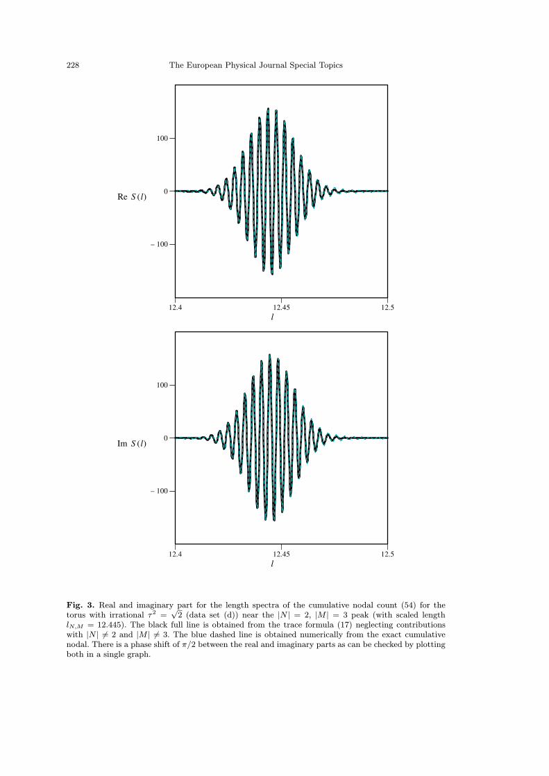
Fig. 3. Real and imaginary part for the length spectra of the cumulative nodal count (54) for thetorus with irrational τ2 =

√2 (data set (d)) near the |N | = 2, |M | = 3 peak (with scaled length

lN,M = 12.445). The black full line is obtained from the trace formula (17) neglecting contributionswith |N | = 2 and |M | = 3. The blue dashed line is obtained numerically from the exact cumulativenodal. There is a phase shift of π/2 between the real and imaginary parts as can be checked by plottingboth in a single graph.


Altogether we define the length spectrum by

S(l) = l3/2∫ ∞0

dκ κ−5/2cosc(K = κ2)e−(κ−κ0)2

ω +iκl. (54)

The final multiplication with l3/2 is not necessary but improves visibilty of peaks in a plot overa large range of lengths l.The trace formula for the cumulative nodal count predicts pronounced peaks at the scaled

lengths l = lr of the periodic geodesics. For the absolute value of the length spectrum these canbe seen very nicely in Fig. 2 which shows a remarkable agreement of the numerical data withthe theoretical predictions.Not only the absolute value of the length spectrum is recovered by the trace formula but also

its phase. This can be seen in fig. 3 where the real and imaginary parts of the length spectrumof the torus with τ2 =

√2 (data set (d)) are plotted near the peak corresponding to periodic

motion with winding numbers (|N |, |M |) = (2, 3).This excellent agreement provides further support for the validity of the approximations

which were used in the derivation of the two versions of the nodal counts trace formula.

This work was supported by the Minerva Center for non-linear Physics and the Einstein (Minerva)Center at the Weizmann Institute, and by grants from the GIF (grant I-808-228.14/2003), and EPSRC(grant GR/T06872/01).

References

1. E.F.F. Chladni, Die Akustik (Breitkopf and Hartel, Leipzig, 1802)2. D. Jakobson, N. Nadirashvili, J. Thot, Russ. Math. Surv. 56, 1085 (2001)3. R. Courant, D. Hilbert, Methods of Mathematical Physics, Vol. I (Interscience, New York, 1953),p. 451

4. G. Blum, S. Gnutzmann, U. Smilansky, Phys. Rev. Lett. 88, 114101 (2002)5. E. Bogomolny, C. Schmit, Phys. Rev. Lett. 88, 114102 (2002)6. E. Bogomolny, R. Dubertrand, C. Schmit, nlin.CD/0609017 (2006)7. J. Keating, J. Marklof, I. Williams, Phys. Rev. Lett. 97, 034101 (2006)8. S. Gnutzmann, U. Smilansky, N. Sondergaard, J. Phys. A 38, 8921 (2005)9. S. Gnutzmann, U. Smilansky, P. Karageorge, Phys. Rev. Lett. 97, 090201 (2006)10. M. Kac, Amer. Math. Monthly 73, part II, 1 (1966)11. R. Band, T. Shapira, U. Smilansky, J. Phys. A 39, 13999 (2006)12. M. Berry, M. Tabor, Proc. Roy. Soc. Lond. Ser. A 356, 375 (1977)13. Y. Colin de Verdiere, Math. Z. 171, 51 (1980)14. P.M. Bleher, Z. Cheng, F.J. Dyson, J.L. Lebowitz, Commun. Math. Phys. 154, 433 (1993)15. P.M. Bleher, Duke Math. J. 74, 45 (1994)

A trace formula for the nodal count sequence

Documents