A time- and space-optimal algorithm for the many-visits TSP

A time- and space-optimal algorithm for the many-visits TSP∗

Andre Berger† Laszlo Kozma‡ Matthias Mnich§ Roland Vincze¶

AbstractThe many-visits traveling salesperson problem (MV-TSP) asks for an optimal tour of n

cities that visits each city c a prescribed number kc of times. Travel costs may be asymmetric,and visiting a city twice in a row may incur a non-zero cost. The MV-TSP problem findsapplications in scheduling, geometric approximation, and Hamiltonicity of certain graphfamilies.

The fastest known algorithm for MV-TSP is due to Cosmadakis and Papadimitriou(SICOMP, 1984). It runs in time nO(n) + O(n3 log

∑c kc) and requires nΩ(n) space. The

interesting feature of the Cosmadakis-Papadimitriou algorithm is its logarithmic dependenceon the total length

∑c kc of the tour, allowing the algorithm to handle instances with very long

tours, beyond what is tractable in the standard TSP setting. However, its superexponentialdependence on the number of cities in both its time and space complexity renders thealgorithm impractical for all but the narrowest range of this parameter.

In this paper we significantly improve on the Cosmadakis-Papadimitriou algorithm, givingan MV-TSP algorithm that runs in single-exponential time with polynomial space. Moreprecisely, we obtain the run time 2O(n) +O(n3 log

∑c kc), with O(n2 log

∑c kc) space. The

space requirement of our algorithm is (essentially) the size of the output, and assuming theExponential-time Hypothesis (ETH), the time requirement is optimal.

Our algorithm is deterministic, and arguably both simpler and easier to analyse thanthe original approach of Cosmadakis and Papadimitriou. It involves an optimization overdirected spanning trees and a recursive, centroid-based decomposition of trees.

1 Introduction

The traveling salesperson problem (TSP) is one of the cornerstones of combinatorial optimization,with origins going back (at least) to the 19th century work of Hamilton (for surveys on the richhistory, variants, and current status of TSP we refer to the dedicated books [3, 10, 19, 30]). Inthe standard TSP, given n cities and their pairwise distances, we seek a tour of minimum totaldistance that visits each city. If the distances obey the triangle inequality, then an optimal tournecessarily visits each city exactly once (apart from returning to the starting city in the end). Inthe general case of the TSP with arbitrary distances, the optimal tour may visit a city multipletimes. (Instances with non-metric distances arise from various applications that are modeled bythe TSP, e.g. from scheduling problems.)

To date, the fastest known exact algorithms for TSP (both in the metric and non-metriccases) are due to Bellman [6] and Held and Karp [20], running in time 2n · O(n2) for n-cityinstances; both algorithms also require space Ω(2n).

In this paper we study the more general problem where each city has to be visited exactly agiven number of times. More precisely, we are given a set V of n vertices, with pairwise distances∗Research of L.K. supported by ERC Consolidator Grant No 617951. Research of M.M. supported by DFG

Grant MN 59/4-1.†Maastricht University, Department of Quantitative Economics, [email protected]‡Eindhoven University of Technology, Department of Mathematics and Computer Science, [email protected]§Universitat Bonn, Department of Computer Science and Maastricht University, Department of Quantitative

Economics, [email protected]¶Maastricht University, Department of Quantitative Economics, [email protected]

1

(or costs) dij ∈ N ∪ ∞, for all i, j ∈ V . No further assumptions are made on the values dij , inparticular, they may be asymmetric, i.e. dij may not equal dji, and the cost dii of a self-loopmay be non-zero. Also given are integers ki ≥ 1 for i ∈ V , which we refer to as multiplicities. Avalid tour of length k is a sequence (x1, . . . , xk) ∈ V k, where k =

∑i∈V ki, such that each i ∈ V

appears in the sequence exactly ki times. The cost of the tour is∑k−1

i=1 dxi,xi+1 + dxk,x1 . Ourgoal is to find a valid tour with minimum cost.

The problem is known as the many-visits TSP (MV-TSP). (As an alternative name, high-multiplicity TSP also appears in the literature.) It includes the standard metric TSP in thespecial case when k = n (i.e. if ki = 1 for all i ∈ V ) and dij forms a metric, thus it cannot besolved in polynomial time, unless P = NP. Nonetheless, the problem is tractable in the regimeof small n values, even if the length k of the tour is very large (possibly exponential in n).

As a natural TSP-generalization, MV-TSP is a fundamental problem of independent interest.In addition, MV-TSP proved to be useful for modeling other problems, particularly in schedul-ing [7, 22, 35, 38]. Suppose there are k jobs of n different types to be executed on a single,universal machine. Processing a job, as well as switching to another type of job come withcertain costs, and the goal is to find the sequence of jobs with minimal total cost. Modeling thisproblem as a MV-TSP instance is straightforward, by letting dij denote the cost of processing ajob of type i together with the cost of switching from type i to type j. Emmons and Mathur [14]also describe an application of MV-TSP to the no-wait flow shop problem.

A different kind of application comes from geometric approximation. To solve geometricoptimization problems approximately, it is a standard technique to reduce the size of the inputby grouping certain input points together. Each group is then replaced by a single representative,and the reduced instance is solved exactly. (For instance, we may snap input points to nearbygrid points, if doing so does not significantly affect the objective cost.) Recently, this techniquewas used by Kozma and Momke, to give an efficient polynomial-time approximation scheme(EPTAS) for the Maximum Scatter TSP in doubling metrics [28], addressing an open questionof Arkin et al. [4]. In this case, the reduced problem is exactly the MV-TSP. Yet anotherapplication of MV-TSP is in settling the parameterized complexity of finding a Hamiltoniancycle in a graph class with restricted neighborhood structure [29].

To the best of our knowledge, MV-TSP was first considered in 1966 by Rothkopf [36]. In1980, Psaraftis [35] gave a dynamic programming algorithm with run time O(n2 ·

∏i∈V (ki + 1)).

Observe that this quantity may be as high as (k/n+1)n, which is prohibitive even for moderatelylarge values of k. In 1984, Cosmadakis and Papadimitriou [12] observed that MV-TSP can bedecomposed into a connectivity subproblem and an assignment subproblem. Taking advantageof this decomposition, they designed a family of algorithms, the best of which has run timeO∗(n2n2n + log k).1 The result can be seen as an early example of fixed-parameter tractability,where the rapid growth in complexity is restricted to a certain parameter.

The algorithm of Cosmadakis and Papadimitriou is, to date, the fastest solution to MV-TSP.2Its analysis is highly non-trivial, combining graph-theoretic insights and involved estimates ofvarious combinatorial quantities. The upper bound is not known to be tight, but the analysisappears difficult to improve, and a lower bound of Ω(nn) is known to hold. Similarly, in thespace requirement of the algorithm, a term of the form nΩ(n) appears hard to avoid.

While it extends the tractability of TSP to a new range of parameters, the usefulness of theCosmadakis-Papadimitriou algorithm is limited by its superexponential3 dependence on n in therun time. In some sense, the issue of exponential space is even more worrisome (the survey ofWoeginger [39] goes as far as calling exponential-space algorithms “absolutely useless”).

1Here, and in the following, the O∗(·) notation is used to suppress a low-order polynomial factor in n.2It may seem that a linear dependence on the length k of the tour is necessary even to output the result.

Observe however, that a tour can be compactly represented by collapsing cycles and storing them together withtheir multiplicities.

3In this paper the term superexponential always refers to a quantity of the form nΩ(n).

2

There have been further studies of the MV-TSP problem. Van der Veen and Zhang [38]discuss a problem equivalent to MV-TSP, called K-group TSP, and describe an algorithmwith polylogarithmic dependence on the number k of visits (similarly to Cosmadakis andPapadimitriou). The value n however is assumed constant, and its effect on the run time is notexplicitly computed (the dependence can be seen to be superexponential). Finally, Grigorievand van de Klundert [17] give an ILP formulation for MV-TSP with O(n2) variables. ApplyingKannan’s improvement [25] of Lenstra’s algorithm [31] for solving fixed-dimensional ILPs tothis formulation yields an algorithm with run time nO(n2) · log k. Further ILP formulationsfor MV-TSP are due to Sarin et al. [37] and Aguayo et al. [2], both of which again requiresuperexponential time to be solved by standard algorithms.

For further details about the history of the MV-TSP problem we refer to the TSP textbookof Gutin et al. [19, § 11.10].

Our results. Our main result improves both the time and space complexity of the best knownalgorithm for MV-TSP, the first improvement in over 30 years. Specifically, we show thata logarithmic dependence on the number k of visits, a single-exponential dependence on thenumber n of cities, and a polynomial space complexity are simultaneously achievable. Moreover,while we build upon ideas from the previous best approach, our algorithm is arguably botheasier to describe, easier to implement, and easier to analyse than its predecessor. To introducethe techniques step-by-step, we describe three algorithms for solving MV-TSP. These are calledenum-MV, dp-MV, and dc-MV. We also mention possible practical improvements. All ouralgorithms are deterministic. Their complexities are summarized in Theorem 1.1, proved in § 2.

Theorem 1.1.

(i) enum-MV solves MV-TSP in time O∗(nn + log k) and space O(n2 log k).

(ii) dp-MV solves MV-TSP in time O∗(5n + log k) and space O∗(5n + log k).

(iii) dc-MV solves MV-TSP in time O∗((32 + ε)n + log k) for any ε > 0 and space O(n2 log k).

The Exponential-Time Hypothesis (ETH) [23] implies that TSP cannot be solved in 2o(n),i.e. sub-exponential, time. Under this hypothesis, the run time of our algorithm dc-MV isasymptotically optimal for MV-TSP (up to the base of the exponent). Further note that thespace requirement of dc-MV is also (essentially) optimal, as a compact solution encodes foreach of the Ω(n2) edges the number t of times that this edge is traversed by an optimal tour.

Our result leads to improvements in applications where MV-TSP is solved as a subroutine.For instance, as a corollary of Theorem 1.1, the approximation scheme for Maximum ScatterTSP [28] can now be implemented in space polynomial in the error parameter ε.

It is interesting to contrast our results for MV-TSP with recent results for the r-simplepath problem, where a long path is sought that visits each vertex at most r times. For thatproblem, the fastest known algorithms—due to Abasi et al. [1] and Gabizon et al. [15]—have runtime exponential in the average number of visits, and such exponential dependence is necessaryassuming ETH.

Overview of techniques. The Cosmadakis-Papadimitriou algorithm is based on the followinghigh-level insight, common to most work on the TSP problem, whether exact or approximate.The task of finding a valid tour may be split into two separate tasks: (1) finding a structurethat connects all vertices, and (2) augmenting the structure found in (1) in order to ensure thateach city is visited the required number of times.

Indeed, such an approach is also used, for instance, in the well-known 3/2-approximationalgorithm of Christofides for metric TSP [9]. There, the structure that guarantees connectivityis a minimum spanning tree, and “visitability” is enforced by the addition of a perfect matching

3

that connects odd-degree vertices (ensuring that all vertices have even degree, and can thus beentered and exited, as required).

In the case of MV-TSP, Cosmadakis and Papadimitriou ensure connectivity (part (1)) byfinding a minimal Eulerian digraph on the set V . Indeed, a minimal Eulerian digraph must bepart of every solution, since a tour must balance every vertex (equal out-degree and in-degree),and all vertices must be mutually reachable. Minimality is meant here in the sense that noproper subgraph is Eulerian, and is required only to reduce the search space.

Assuming that an Eulerian digraph is found that is part of the solution, it needs to beextended to a tour in which all vertices are visited the required number of times (part (2)). Ifthis is done with the cheapest possible set of edges, then the optimum must have been found.This second step amounts to solving a transportation problem, which takes polynomial time.

The first step, however, requires us to consider all possible minimal Eulerian digraphs. Asit is NP-complete to test the non-minimality of an Eulerian digraph [34], the authors relaxminimality and suggest the use of heuristics for pruning out non-minimal instances in practice.On the other hand, they obtain a saving in run time by observing that among all Euleriandigraphs with the same degree sequence only the one with smallest cost needs to be considered.(Otherwise, in the final tour, the Eulerian subdigraph could be swapped with a cheaper one,while maintaining the validity of the tour.)

Cosmadakis and Papadimitriou iterate thus over feasible degree sequences of Euleriandigraphs; for each such degree sequence they construct the cheapest Eulerian digraph (whichmay not be minimal) by dynamic programming; finally, for each such Eulerian digraph constructthe cheapest extension to a valid tour (by solving a transportation problem). The returnedsolution is the cheapest tour found over all iterations.

Iterating and optimizing over these structures is no easy task, and Cosmadakis and Papadim-itriou invoke a number of graph-theoretic and combinatorial insights. For estimating the totalcost of their procedure a sophisticated global counting argument is developed.

The key insight of our approach is that the machinery involving Eulerian digraphs is notnecessary for solving MV-TSP. To ensure connectivity (i.e. task (1) above), a directed spanningtree is sufficient. This may seem surprising, as a directed tree fails to satisfy the main propertyof Eulerian digraphs, strong connectivity. Observe however, that a collection of directed edgeswith the same out-degrees and in-degrees as a valid MV-TSP tour is itself a valid tour, unless itconsists of disjoint cycles. Requiring the solution to contain a tree is sufficient to avoid the caseof disjoint cycles. The fact that the tree can be assumed to be rooted (i.e. all of its edges aredirected away from some vertex) follows from the strong connectedness of the tour.4

Directed spanning trees are easier to enumerate and optimize over than minimal Euleriandigraphs; this fact alone explains the reduced complexity of our approach. However, to obtainour main result, further ideas are needed. In particular, we find the cheapest directed spanningtree that is feasible for a given degree sequence, first by dynamic programming, then by arecursive partitioning of trees, based on centroid-decompositions.

Given the fundamental nature of the TSP-family of problems and the remaining openquestions they pose, we hope that our techniques may find further applications.

2 Improved algorithms for the Many-Visits TSP

In this section we describe and analyse our three algorithms. The first, enum-MV is based onexact enumeration of trees (§ 2.2), the second, dp-MV uses a dynamic programming approachto find an optimal tree (§ 2.3), and the third, dc-MV is based on divide and conquer (§ 2.4).Before presenting the algorithms, we introduce some notation and structural observations thatare subsequently used (§ 2.1).

4We thank Andreas Bjorklund for the latter observation which led to an improved run time and a simplercorrectness argument.

4

2.1 Trees, tours, and degree sequences

Let V be a set of vertices. We view directed multigraphs G with vertex set V as multisets ofedges (i.e. elements of V × V ). Accordingly, self-loops and multiple copies of the same edgeare allowed. The multiplicity of an edge (i, j) in a directed multigraph G is denoted mG(i, j).The out-degree of a vertex i ∈ V is δout

G (i) =∑

j∈V mG(i, j), the in-degree of a vertex i ∈ V isδin

G (i) =∑

j∈V mG(j, i). Given edge costs d : V × V → N∪ ∞, the cost of G is simply the sumof its edge costs, i.e. cost(G) =

∑i,j∈V mG(i, j) · d(i, j).

For two directed multigraphs G and H over the same vertex set V , let G+H denote thedirected multigraph obtained by adding the corresponding edge multiplicities of G and H.Observe that as an effect, out-degrees and in-degrees are also added pointwise. Formally,mG+H(i, j) = mG(i, j) +mH(i, j), δout

G+H(i) = δoutG (i) + δout

H (i) and δinG+H(i) = δin

G (i) + δinH(i), for

all i, j ∈ V . The relation cost(G+H) = cost(G) + cost(H) clearly holds.In the following, for a directed multigraph G we refer to its underlying undirected graph, i.e.

to the graph consisting of those edges i, j for which mG(i, j) +mG(j, i) ≥ 1.Consider a tour C = (x1, . . . , xk) ∈ V k. We refer to the unique directed multigraph G

consisting of the edges (x1, x2), . . . , (xk−1, xk), (xk, x1) as the edge set of C. We state a simplebut crucial observation.

Lemma 2.1. Let G be a directed multigraph over V with out-degrees δoutG (·) and in-degrees δin

G (·).Then G is the edge set of a tour that visits each vertex i ∈ V exactly ki times if and only if bothof the following conditions hold:

(i) the underlying undirected graph of G is connected, and

(ii) for all i ∈ V , we have δoutG (i) = δin

G (i) = ki.

Proof. The fact that connectedness of G and δoutG (i) = δin

G (i) is equivalent with the existenceof a tour that uses each edge of G exactly once is the well-known “Euler’s theorem”. (See [5,Thm 1.6.3] for a short proof.) Clearly, visiting each vertex i exactly ki times is equivalent withthe condition that the tour contains ki edges of the form (·, i) and ki edges of the form (i, ·).

Moreover, given the edge set G of a tour C, a tour C ′ with edge set G can easily berecovered. This amounts to finding an Eulerian tour of G, which can be done in time linearin the length k of the tour. To avoid a linear dependence on k, we can apply the algorithmof Grigoriev and van de Klundert [17] that constructs a compact representation of C ′ in timeO(n4 log k). As the edge sets of C and C ′ are equal, C ′ also visits each i ∈ V exactly ki timesand cost(C ′) = cost(C) = cost(G).

Thus, in solving MV-TSP we only focus on finding a directed multigraph whose underlyingundirected graph is connected, and whose degrees match the multiplicities required by theproblem.

A directed spanning tree of V is a tree with vertex set V whose edges are directed away fromsome vertex r ∈ V ; in other words, the tree contains a directed path from r to every other vertexin V . (Directed spanning trees are alternatively called branchings, arborescences, or out-trees.)We refer to the vertex r as the root of the tree. We observe that every valid tour contains adirected spanning tree.

Lemma 2.2. Let G be the edge set of a tour of V (with arbitrary non-zero multiplicities), andlet r ∈ V be an arbitrary vertex. Then there is a directed spanning tree T of G and a directedmultigraph X such that G = T +X.

Proof. We choose T to be the single-source shortest path tree in G with source r. More precisely,let Px be the edge set of the shortest path from r to x in G for all x ∈ V \ r . (In a valid tourall vertices are mutually reachable.) In case of ties, we choose the path that is alphabeticallysmaller. Let T =

⋃x∈V \r Px, i.e. the union of all shortest paths. The fact that T is a directed

tree with root r is a direct consequence of the definition of shortest paths (see e.g. [11, § 24]).

5

We can thus split the MV-TSP problem into finding a directed spanning tree T with anarbitrary root r and an extension X, such that T + X is a valid tour. We claim that in thedecomposition G = T + X of an optimal tour G, both T and X are optimal with respect totheir degree sequences.

Lemma 2.3. Let G be the edge set of an optimal tour for MV-TSP, let T be a directed spanningtree, and X a directed multigraph such that G = T +X. Then, among all directed spanning treeswith degrees δout

T (·), δinT (·), T is of minimal cost. Among all directed multigraphs with degrees

δoutX (·), δin

X(·), X is of minimal cost.

Proof. Suppose there is a directed spanning tree T ′ such that cost(T ′) < cost(T ) and δoutT ′ (i) =

δoutT (i), δin

T ′(i) = δinT (i) for all i ∈ V . But then T ′+X is connected, has the same degree sequence

as G, while cost(T ′ +X) < cost(G), contradicting the optimality of G.Similarly, suppose there is a directed multigraph X ′ such that cost(X ′) < cost(X) and

δoutX′ (i) = δout

X (i), δinX′(i) = δin

X(i) for all i ∈ V . But then T +X ′ is connected, has the same degreesequence as G, while cost(T +X ′) < cost(G), contradicting the optimality of G.

Next, we characterize the feasible degree sequences of directed spanning trees.

Lemma 2.4. Let V = x1, . . . , xn be a set of vertices. There is a directed spanning tree of Vwith root x1 whose out-degrees and in-degrees are respectively δout(·) and δin(·), if and only if

(i) δin(x1) = 0,

(ii) δin(xi) = 1 for every 1 < i ≤ n,

(iii) δout(x1) > 0, and

(iv)∑

i δout(xi) = n− 1.

Proof. In the forward direction, in a directed spanning tree all non-root vertices have exactlyone parent, proving (i) and (ii). The root must have at least one child (iii), and the total numberof edges is n− 1, proving (iv).

In the backward direction, we argue by induction on n. In the case n = 2, we haveδin(x1) = δout(x2) = 0, and δin(x2) = δout(x1) = 1, hence an edge (x1, x2) satisfies the degreerequirements.

Consider now the case of n > 2 vertices. From (ii)–(iv) it follows that for some k, 1 < k ≤ n,we have δin(xk) = 1 and δout(xk) = 0, i.e. xk is a leaf.

Let j, 1 ≤ j ≤ n, j 6= k, such that δout(xj) ≥ 1 and δin(xj) + δout(xj) ≥ 2; by (ii)–(iv)there must be such a vertex. We decrease δout(xj) by one. Conditions (i)–(iv) clearly hold forV \ xk. By induction, we can build a tree on V \ xk, and attach xk to this tree as a leaf,with the edge (xj , xk).

Let DS(n) denote the number of different pairs of sequences (δ′1, . . . , δ′n), (δ′′1 , . . . , δ′′n), thatare feasible for a directed spanning tree, i.e. for vertex set V = x1, . . . , xn, for some directedspanning tree T with root x1, we have δout

T (xi) = δ′i, and δinT (xi) = δ′′i , for all i ∈ 1, . . . , n. By

Lemma 2.4, DS(n) equals the number of ways to distribute n− 1 out-degrees to n vertices, suchthat a designated vertex has non-zero out-degree. This is the same as distributing n− 2 ballsarbitrarily into n bins, of which there are

(2n−3n−1

)= O(4n) ways.

2.2 enum-MV: polynomial space and superexponential time

Given a vertex set V with |V | = n, multiplicities ki ∈ N and cost function d, we wish to find atour of minimum cost that visits each i ∈ V exactly ki times.

6

From Lemma 2.2, our first algorithm presents itself. It simply iterates over all directedspanning trees T with vertex set V , and extends each of them optimally to a valid tour CT .Among all valid tours constructed, the one with smallest cost is returned (Algorithm 1).

This simple algorithm already improves on the previous best run time (although it is stillsuperexponential), and reduces the space requirement from superexponential to polynomial.

Algorithm 1 enum-MV for solving MV-TSP using enumerationInput: Vertex set V , cost function d, multiplicities ki.Output: A tour of minimum cost that visits each i ∈ V exactly ki times.

1: for each directed spanning tree T with root r ∈ V do2: Find minimum cost directed multigraph X such that for all i ∈ V :

δoutX (i) := ki − δout

T (i),δin

X(i) := ki − δinT (i).

Denote CT := T +X.3: return CT with smallest cost.

The correctness of the algorithm is immediate: from Lemma 2.2 it follows that all CT ’sconsidered are valid (connected, and with degrees matching the required multiplicities), and byLemma 2.3, the optimal tour C must be considered during the execution.

The iteration of Line 1 requires us to enumerate all labeled trees with vertex set V . Thereare nn−2 such trees [8], and standard techniques can be used to enumerate them with a constantoverhead per item (see e.g. Kapoor and Ramesh [26]). For each considered tree we orient theedges in a unique way (away from r).

Let T be the current tree. In Line 2 we need to find a minimum cost directed multigraph X,with given out-degree and in-degree sequence (such as to extend T into a valid tour). If, forsome vertex i, it holds that δin

T (i) > ki or δoutT (i) > ki, we proceed to the next spanning tree,

since the current tree cannot be extended to a valid tour. Observe that this may happen only ifki < n− 1, for some i ∈ V .

Otherwise, we find the optimal X by solving a transportation problem in polynomial time.During the algorithm we maintain the current best tour, which we output in the end. Wedescribe next the transportation subroutine, which is common to all our algorithms, and isessentially the same as in the Cosmadakis-Papadimitriou algorithm.

The transportation problem. The subproblem we need to solve is to find a minimum costdirected multigraph X over vertex set V , with given out-degree and in-degree requirements.

We can map this problem to an instance of the Hitchcock transportation problem [21], wherethe goal is to transport a given amount of goods from N warehouses to M outlets with givenpairwise shipping costs. (This is a special case of the more general min-cost max-flow problem.)The transportation problem can be solved in polynomial time using the scaling method ofEdmonds and Karp [13].

More precisely, let us define a digraph with vertices s, t ∪ si, ti | i ∈ V . Edges are(s, si), (ti, t) | i ∈ V , and (si, tj) | i, j ∈ V . We set cost 0 to edges (s, si) and (ti, t)and cost dij (i.e. the costs given in the MV-TSP instance) to (si, tj). We set capacity ∞ toedges (si, tj) and capacities ki − δout

T (i) to (s, si), and ki − δinT (i) to (ti, t). The construction is

identical to the one used by Cosmadakis and Papadimitriou, apart from the fact that in ourcase the capacity of (s, si) may be different from the capacity of (ti, t). Observe that the sumof capacities of (s, si)-edges equals the sum of capacities of (ti, t)-edges over all i ∈ V . Thus, amaximal s− t flow saturates all these edges.

The amount of flow transmitted on the edge (si, tj) gives the multiplicity of edge (i, j) inthe sought after multigraph, for all i, j ∈ V . A minimum cost maximum flow clearly maps to aminimum cost edge set with the given degree constraints.

7

The Edmonds-Karp algorithm proceeds by solving O(log k) approximate versions of theproblem, where the costs are the same as in the original problem, but the capacities are scaledby a factor 2p for p = dlog ke, . . . , 0. Each approximate problem is solved by performing flowaugmentations on the optimal flow found in the previous approximation (multiplied by two).Each approximation can be solved in O(n3) time. Therefore, the run time of the Edmonds-Karpscaling algorithm for solving the described transportation problem is O(n3 · log k).

Cosmadakis and Papadimitriou describe an improvement which also applies for our case.Namely, they show that the total run time for solving several instances with the same costs canbe reduced, if the capacities on corresponding edges in two different instances may differ by atmost n.

The strategy is to solve all but the last logn approximate problems only once, as these are(essentially) the same for all instances. For different instances we only need to solve the lastlogn approximate problems (i.e. at the finest levels of approximation). This gives a run timeof O(n3 · log k) for solving the “master problem”, and O(n3 · logn) for solving each individualinstance. (We refer to Cosmadakis and Papadimitriou [12] as well as Edmonds and Karp [13]for details.)

In our case, the different instances of the transportation problem are for finding the directedmultigraphs X for different trees T . Each of these instances agree in the underlying graph andcost function, and may differ only in the capacities. As the maximum degree of each tree T is atmost n− 1, the differences are bounded, as required.

Analysis of the algorithm. We iterate over all O(nn−2) directed spanning trees and solve atransportation problem for each, with run time O(n3 · log k). The total run time O(nn+1 · log k)follows. With the described improvement w.r. to solving a master-problem in advance, weimprove this to O(nn+1 · logn+ n3 · log k).

The algorithm only needs to store the edge set of a single tour (apart from minor bookkeeping),with space complexity O(n2 · log k).

2.2.1 Improved enumeration algorithm

We can improve the run time of enum-MV by observing that the solution of the transportationproblem depends only on the degree sequence of the current tree T , and not the actual edgesof T . Therefore, different trees with the same degree sequence can be extended in the sameway. (Several trees may have the same degree sequence; in an extreme case, all (n− 2)! simpleHamiltonian paths with the same endpoints have the same degree sequence.) Algorithm 2implements this idea, iterating over all trees, grouped by their degree sequences. It solves thetransportation problem only once for each degree sequence (there are DS(n) of them).

Algorithm 2 enum-MV for solving MV-TSP using enumeration (improved)Input: Vertex set V , cost function d, multiplicities ki.Output: A tour of minimum cost that visits each i ∈ V exactly ki times.

1: for each feasible degree sequence δout(·), δin(·) of a directed spanning tree with root r do2: for each directed spanning tree T with δout

T = δout, δinT = δin do

3: Find minimum cost directed multigraph X such that for all i ∈ V :δout

X (i) := ki − δoutT (i),

δinX(i) := ki − δin

T (i).Denote CT := T +X.

4: return CT with smallest cost.

The correctness is immediate, as all directed spanning trees T are still considered, as before.Assume that we can iterate over all feasible degree sequences, and all corresponding trees with

8

constant overhead per item. By Lemma 2.4, the first task only requires us to consider all waysof distributing n− 2 out-degrees among n vertices. For completeness, we describe the procedurethat achieves this with O(n) overhead per item, in Appendix A. We give the subroutine for thesecond task in § 2.2.2.) We thus obtain the run time O(nn−1 + DS(n) · n4 · log k). Using thesame technique of solving a master-problem in advance, the bound O(nn−1 + n3 · log k) follows.The space requirement is asymptotically unchanged.

2.2.2 Generating trees by degree sequence

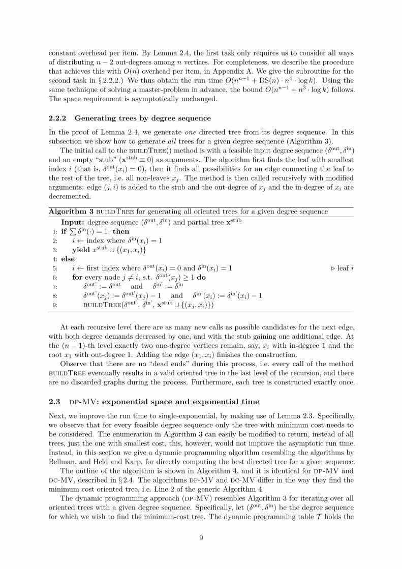
In the proof of Lemma 2.4, we generate one directed tree from its degree sequence. In thissubsection we show how to generate all trees for a given degree sequence (Algorithm 3).

The initial call to the buildTree() method is with a feasible input degree sequence (δout, δin)and an empty “stub” (xstub ≡ 0) as arguments. The algorithm first finds the leaf with smallestindex i (that is, δout(xi) = 0), then it finds all possibilities for an edge connecting the leaf tothe rest of the tree, i.e. all non-leaves xj . The method is then called recursively with modifiedarguments: edge (j, i) is added to the stub and the out-degree of xj and the in-degree of xi aredecremented.

Algorithm 3 buildTree for generating all oriented trees for a given degree sequenceInput: degree sequence (δout, δin) and partial tree xstub

1: if∑δin(·) = 1 then

2: i← index where δin(xi) = 13: yield xstub ∪ (x1, xi)4: else5: i← first index where δout(xi) = 0 and δin(xi) = 1 . leaf i6: for every node j 6= i, s.t. δout(xj) ≥ 1 do7: δout’ := δout and δin’ := δin

8: δout’(xj) := δout’(xj)− 1 and δin’(xi) := δin’(xi)− 19: buildTree(δout’, δin’, xstub ∪ (xj , xi))

At each recursive level there are as many new calls as possible candidates for the next edge,with both degree demands decreased by one, and with the stub gaining one additional edge. Atthe (n − 1)-th level exactly two one-degree vertices remain, say, xi with in-degree 1 and theroot x1 with out-degree 1. Adding the edge (x1, xi) finishes the construction.

Observe that there are no “dead ends” during this process, i.e. every call of the methodbuildTree eventually results in a valid oriented tree in the last level of the recursion, and thereare no discarded graphs during the process. Furthermore, each tree is constructed exactly once.

2.3 dp-MV: exponential space and exponential time

Next, we improve the run time to single-exponential, by making use of Lemma 2.3. Specifically,we observe that for every feasible degree sequence only the tree with minimum cost needs tobe considered. The enumeration in Algorithm 3 can easily be modified to return, instead of alltrees, just the one with smallest cost, this, however, would not improve the asymptotic run time.Instead, in this section we give a dynamic programming algorithm resembling the algorithms byBellman, and Held and Karp, for directly computing the best directed tree for a given sequence.

The outline of the algorithm is shown in Algorithm 4, and it is identical for dp-MV anddc-MV, described in § 2.4. The algorithms dp-MV and dc-MV differ in the way they find theminimum cost oriented tree, i.e. Line 2 of the generic Algorithm 4.

The dynamic programming approach (dp-MV) resembles Algorithm 3 for iterating over alloriented trees with a given degree sequence. Specifically, let (δout, δin) be the degree sequencefor which we wish to find the minimum-cost tree. The dynamic programming table T holds the

9

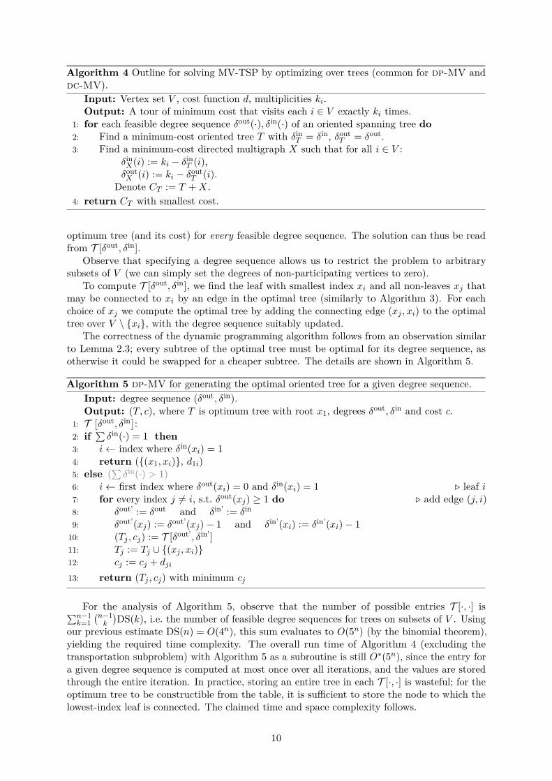
Algorithm 4 Outline for solving MV-TSP by optimizing over trees (common for dp-MV anddc-MV).

Input: Vertex set V , cost function d, multiplicities ki.Output: A tour of minimum cost that visits each i ∈ V exactly ki times.

1: for each feasible degree sequence δout(·), δin(·) of an oriented spanning tree do2: Find a minimum-cost oriented tree T with δin

T = δin, δoutT = δout.

3: Find a minimum-cost directed multigraph X such that for all i ∈ V :δin

X(i) := ki − δinT (i),

δoutX (i) := ki − δout

T (i).Denote CT := T +X.

4: return CT with smallest cost.

optimum tree (and its cost) for every feasible degree sequence. The solution can thus be readfrom T [δout, δin].

Observe that specifying a degree sequence allows us to restrict the problem to arbitrarysubsets of V (we can simply set the degrees of non-participating vertices to zero).

To compute T [δout, δin], we find the leaf with smallest index xi and all non-leaves xj thatmay be connected to xi by an edge in the optimal tree (similarly to Algorithm 3). For eachchoice of xj we compute the optimal tree by adding the connecting edge (xj , xi) to the optimaltree over V \ xi, with the degree sequence suitably updated.

The correctness of the dynamic programming algorithm follows from an observation similarto Lemma 2.3; every subtree of the optimal tree must be optimal for its degree sequence, asotherwise it could be swapped for a cheaper subtree. The details are shown in Algorithm 5.

Algorithm 5 dp-MV for generating the optimal oriented tree for a given degree sequence.Input: degree sequence (δout, δin).Output: (T, c), where T is optimum tree with root x1, degrees δout, δin and cost c.

1: T[δout, δin]:

2: if∑δin(·) = 1 then

3: i← index where δin(xi) = 14: return ((x1, xi), d1i)5: else (

∑δin(·) > 1)

6: i← first index where δout(xi) = 0 and δin(xi) = 1 . leaf i7: for every index j 6= i, s.t. δout(xj) ≥ 1 do . add edge (j, i)8: δout’ := δout and δin’ := δin

9: δout’(xj) := δout’(xj)− 1 and δin’(xi) := δin’(xi)− 110: (Tj , cj) := T [δout’, δin’]11: Tj := Tj ∪ (xj , xi)12: cj := cj + dji

13: return (Tj , cj) with minimum cj

For the analysis of Algorithm 5, observe that the number of possible entries T [·, ·] is∑n−1k=1

(n−1k

)DS(k), i.e. the number of feasible degree sequences for trees on subsets of V . Using

our previous estimate DS(n) = O(4n), this sum evaluates to O(5n) (by the binomial theorem),yielding the required time complexity. The overall run time of Algorithm 4 (excluding thetransportation subproblem) with Algorithm 5 as a subroutine is still O∗(5n), since the entry fora given degree sequence is computed at most once over all iterations, and the values are storedthrough the entire iteration. In practice, storing an entire tree in each T [·, ·] is wasteful; for theoptimum tree to be constructible from the table, it is sufficient to store the node to which thelowest-index leaf is connected. The claimed time and space complexity follows.

10

2.4 dc-MV: polynomial space and exponential time

Finally, we show how to reduce the space complexity to polynomial, while maintaining asingle-exponential run time.

The outer loop (Algorithm 4) remains the same, but we replace the subroutine for finding anoptimal directed spanning tree (Algorithm 5) with an approach based on divide and conquer(Algorithm 6). The approach is inspired by the algorithm of Gurevich and Shelah [18] for findingan optimal TSP tour.

The algorithm relies on the following observation about tree-separators. Let (V1, V2) be apartition of V , i.e. V1 ∪ V2 = V , and V1 ∩ V2 = ∅, and let |V | = n. We say that (V1, V2) isbalanced if bn/3c ≤ |V1|, |V2| ≤ d2n/3e.

Lemma 2.5. For every tree T with edge set V , there is a balanced partition (V1, V2) of V suchthat all edges of T between V1 and V2 are incident to a vertex v ∈ V1.

Proof. A very old result of Jordan [24] states that every tree has a centroid vertex, i.e. a vertexwhose removal splits the tree into subtrees not larger than half the original tree. (To find such acentroid, move from an arbitrary vertex, one edge at a time, towards the largest subtree).

Let T1, . . . , Tm be the vertex sets of the trees, in decreasing order of size, resulting fromdeleting the centroid of T . Let e1, . . . , em denote the edges that connect the respective treesto the centroid in T . If |T1| ≥ bn/3c, then we have the balanced partition (V \ T1, T1), with asingle crossing edge.

Otherwise, let m′ be the smallest index such that bn/3c ≤ |T1| + · · · + |Tm′ | ≤ d2n/3e.(As |Ti| < bn/3c for all i, such an index m′ must exist.) Now the balanced partition is(V \ (T1 ∪ · · · ∪ Tm′), T1 ∪ · · · ∪ Tm′). The partition fulfils the stated condition as all crossingedges are incident to the centroid, which is on the left side.

At a high-level, dc-MV works as follows. It “guesses” the partition (V1, V2) of vertexset V according to a balanced separator of the (unknown) optimal rooted tree T , satisfying theconditions of Lemma 2.5. It also “guesses” the distinguished vertex v ∈ V1 to which all edgesthat cross the partition are incident.

The balanced separator splits T into a tree with vertex set V1 and a forest with vertex set V2.There are two cases to consider, depending on whether the root r = x1 of T falls in V1 or V2.

In the first case, V1 induces a directed subtree of T rooted at r, in the second case, V1 inducesa directed subtree of T rooted at v.

Observe that the out-degrees and in-degrees of vertices in V1 are feasible for a directed tree,except for vertex v which has additional degrees due to the edges crossing the partition (we referto these out-degrees and in-degrees as the excess of v). The excess of v can be computed fromLemma 2.4. This excess determines the number and orientation of edges across the cut (even ifthe endpoints, other than v, of the edges are unknown).

By the same argument as in Lemma 2.3, the subtree of T induced by V1 is optimal for itscorresponding degree sequence (after subtracting the excess of v), therefore we can find it by arecursive call to the procedure.

On the other side of the partition we have a collection of trees. To obtain an instance ofour original problem, we add a virtual vertex w to V2 (that plays the role of v). We set theout-degree and in-degree of w to the excess of v, to allow it to connect to all vertices of V2 that vconnects to in T . Now we can find the optimal tree on this side too, by a recursive call to theprocedure.

On both sides, the roots of the directed trees are uniquely determined by the remainingdegrees. Observe that if the original root coincides with the centroid v, then v and w will be theroots of the trees in the recursive calls.

After obtaining the optimal trees on the two sides (assuming the guesses were correct),we reconstruct T by gluing the two trees together, identifying the vertices v and w. As this

11

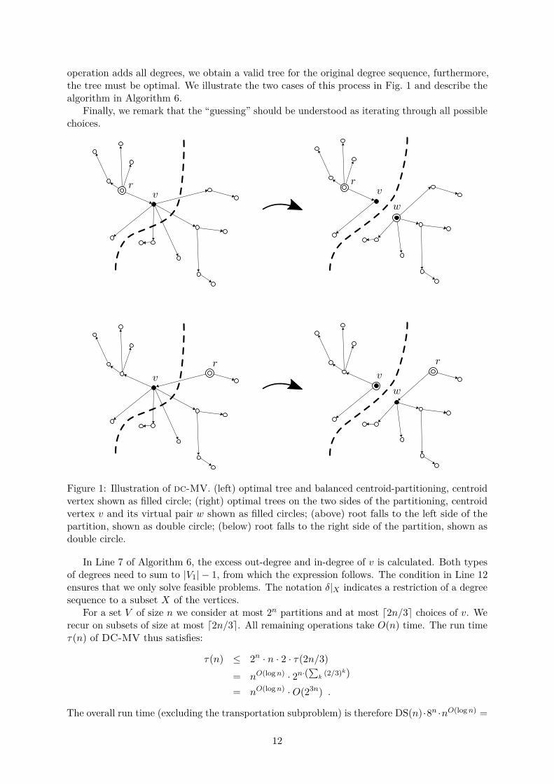
operation adds all degrees, we obtain a valid tree for the original degree sequence, furthermore,the tree must be optimal. We illustrate the two cases of this process in Fig. 1 and describe thealgorithm in Algorithm 6.

Finally, we remark that the “guessing” should be understood as iterating through all possiblechoices.

Figure 1: Illustration of dc-MV. (left) optimal tree and balanced centroid-partitioning, centroidvertex shown as filled circle; (right) optimal trees on the two sides of the partitioning, centroidvertex v and its virtual pair w shown as filled circles; (above) root falls to the left side of thepartition, shown as double circle; (below) root falls to the right side of the partition, shown asdouble circle.

In Line 7 of Algorithm 6, the excess out-degree and in-degree of v is calculated. Both typesof degrees need to sum to |V1| − 1, from which the expression follows. The condition in Line 12ensures that we only solve feasible problems. The notation δ|X indicates a restriction of a degreesequence to a subset X of the vertices.

For a set V of size n we consider at most 2n partitions and at most d2n/3e choices of v. Werecur on subsets of size at most d2n/3e. All remaining operations take O(n) time. The run timeτ(n) of DC-MV thus satisfies:

τ(n) ≤ 2n · n · 2 · τ(2n/3)

= nO(log n) · 2n·(∑

k(2/3)k)

= nO(log n) ·O(23n) .

The overall run time (excluding the transportation subproblem) is therefore DS(n) ·8n ·nO(log n) =

12

Algorithm 6 dc-MV for generating the optimal oriented tree for a given degree sequence.Input: degree sequence

(δout, δin), vertex set V

Output: (T, c), where T is optimum tree for δout, δin and c is its costT[V, δout, δin] :

1: if |V | ≤ 3 then2: directly find optimum tree T with cost c3: return (T , c)4: else5: for each partition (V1, V2) of V , such that |V1|, |V2| ≤ d2n/3e do6: for each v ∈ V1 do7: excessout

v := |V1| − 1−∑

p∈V1p 6=v

δout(p) and excessinv := |V1| − 1−

∑p∈V1p 6=v

δin(p)

8: δout’ := δout and δin’ := δin

9: δout’(v) := δout’(v)− excessoutv and δin’(v) := δin’(v)− excessin

v

10: V ′2 := V2 ∪ w11: δout’(w) := excessout

v and δin’(w) := excessinv

12: if δout’(·), δin’(·) ≥ 0 and δout’(v) + δin’(v) ≥ 1 and δout’(w) + δin’(w) ≥ 1 then13: c1 := T

[V1, δout’|V1 , δin’|V1

]14: c2 := T

[V ′2 , δout’|V ′2 , δin’|V ′2

]15: c := c1 + c216: T ← merge T1 and T2 by identifying v and w

17: return (T, c) with minimum c

O((32 + ε)n), for any ε > 0. For the space complexity, observe that as we do not precomputeT [·, ·], only a single tour is stored at each time, spread over O(logn) recursive levels. The claimedbounds follow.

3 Discussion

We describe three new algorithms for the many-visits TSP problem. In particular, we show howto solve the many-visits TSP problem in time single-exponential in the number n of cities andlogarithmic in the multiplicities, while using space only polynomial in n. This yields the firstimprovement over the Cosmadakis-Papadimitriou algorithm in more than 30 years.

It remains an interesting open question to improve the bases of the exponents in our runtimes; recent algebraic techniques [16, 27, 32] may be of help. An algorithm solving MV-TSP intime O∗(2n · log k), i.e. matching the best known upper bounds for solving the standard TSP,would be particularly interesting, even in the special case when all edge costs are equal to 1 or 2.(Such instances of MV-TSP arise e.g. in the Maximum Scatter TSP application by Kozmaand Momke [28].)

In practice, one may reduce the search space of our algorithms via heuristics, for instance byforcing certain (directed) edges to be part of the solution. An edge (i, j) is part of the solutionif the optimal tour visits it at least once. This may be reasonable if the edge in question arevery cheap.

13

References

[1] H. Abasi, N. H. Bshouty, A. Gabizon, and E. Haramaty. On r-simple k-path. In Proc.MFCS 2014, pages 1–12, 2014.

[2] M. M. Aguayo, S. C. Sarin, and H. D. Sherali. Single-commodity flow-based formulationsand accelerated Benders algorithms for the high-multiplicity asymmetric traveling salesmanproblem and its extensions. J. Oper. Res. Soc., 69(5):734–746, 2018.

[3] D. L. Applegate, R. E. Bixby, V. Chvatal, and W. J. Cook. The Traveling SalesmanProblem: A Computational Study. Princeton University Press, 2006.

[4] E. M. Arkin, Y. Chiang, J. S. B. Mitchell, S. Skiena, and T. Yang. On the maximum scattertraveling salesperson problem. SIAM J. Comput., 29(2):515–544, 1999.

[5] J. Bang-Jensen and G. Z. Gutin. Digraphs - theory, algorithms and applications. Springer,2002.

[6] R. Bellman. Dynamic programming treatment of the travelling salesman problem. J. Assoc.Comput. Mach., 9:61–63, 1962.

[7] N. Brauner, Y. Crama, A. Grigoriev, and J. van de Klundert. A framework for the complexityof high-multiplicity scheduling problems. J. Combinatorial Optim., 9(3):313–323, 2005.

[8] A. Cayley. A theorem on trees. Quart. J. Pure Appl. Math., 23:376–378, 1889.

[9] N. Christofides. Worst-case analysis of a new heuristic for the travelling salesman problem.Technical report, Technical Report 388, Carnegie Mellon University, 1976.

[10] W. Cook. In Pursuit of the Traveling Salesman: Mathematics at the Limits of Computation.Princeton University Press, 2011.

[11] T. H. Cormen, C. E. Leiserson, R. L. Rivest, and C. Stein. Introduction to Algorithms. TheMIT Press, 3rd edition, 2009.

[12] S. S. Cosmadakis and C. H. Papadimitriou. The traveling salesman problem with manyvisits to few cities. SIAM J. Comput., 13(1):99–108, 1984.

[13] J. Edmonds and R. M. Karp. Theoretical improvements in algorithmic efficiency for networkflow problems. In Combinatorial Structures and their Applications (Proc. Calgary Internat.Conf., Calgary, Alta., 1969), pages 93–96. Gordon and Breach, New York, 1970.

[14] H. Emmons and K. Mathur. Lot sizing in a no-wait flow shop. Oper. Res. Lett., 17(4):159–164, 1995.

[15] A. Gabizon, D. Lokshtanov, and M. Pilipczuk. Fast algorithms for parameterized problemswith relaxed disjointness constraints. In Proc. ESA 2015, pages 545–556, 2015.

[16] A. Golovnev. Approximating asymmetric TSP in exponential time. Int. J. Found. Comput.Sci., 25(1):89–100, 2014.

[17] A. Grigoriev and J. van de Klundert. On the high multiplicity traveling salesman problem.Discrete Optim., 3(1):50–62, 2006.

[18] Y. Gurevich and S. Shelah. Expected computation time for Hamiltonian path problem.SIAM J. Comput., 16(3):486–502, 1987.

14

[19] G. Gutin and A. Punnen. The Traveling Salesman Problem and Its Variations. Springer,2002.

[20] M. Held and R. M. Karp. A dynamic programming approach to sequencing problems. J.Soc. Indust. Appl. Math., 10:196–210, 1962.

[21] F. L. Hitchcock. The distribution of a product from several sources to numerous localities.J. Math. Phys. Mass. Inst. Tech., 20:224–230, 1941.

[22] D. S. Hochbaum and R. Shamir. Strongly polynomial algorithms for the high multiplicityscheduling problem. Oper. Res., 39(4):648–653, 1991.

[23] R. Impagliazzo, R. Paturi, and F. Zane. Which problems have strongly exponentialcomplexity? J. Comput. Syst. Sci., 63(4):512–530, 2001.

[24] C. Jordan. Sur les assemblages de lignes. Journal fur die reine und angewandte Mathematik,70:185–190, 1869.

[25] R. Kannan. Improved algorithms for integer programming and related lattice problems. InProc. STOC 1983, pages 193–206, 1983.

[26] S. Kapoor and H. Ramesh. Algorithms for enumerating all spanning trees of undirectedand weighted graphs. SIAM J. Comput., 24(2):247–265, 1995.

[27] M. Koivisto and P. Parviainen. A space-time tradeoff for permutation problems. In Proc.SODA 2010, pages 484–492, 2010.

[28] L. Kozma and T. Momke. Maximum scatter TSP in doubling metrics. In Proc. SODA 2017,pages 143–153, 2017.

[29] M. Lampis. Algorithmic meta-theorems for restrictions of treewidth. Algorithmica, 64(1):19–37, 2012.

[30] E. Lawler, D. Shmoys, A. Kan, and J. Lenstra. The Traveling Salesman Problem. JohnWiley & Sons, 1985.

[31] H. W. Lenstra, Jr. Integer programming with a fixed number of variables. Math. Oper.Res., 8(4):538–548, 1983.

[32] D. Lokshtanov and J. Nederlof. Saving space by algebraization. In Proc. STOC 2010, pages321–330, 2010.

[33] A. Nijenhuis and H. S. Wilf. Combinatorial algorithms. Academic Press, Inc. [HarcourtBrace Jovanovich, Publishers], New York-London, second edition, 1978.

[34] C. H. Papadimitriou and M. Yannakakis. On minimal eulerian graphs. Inf. Proc. Lett., 12(4):203–205, 1981.

[35] H. N. Psaraftis. A dynamic programming approach for sequencing groups of identical jobs.Oper. Res., 28(6):1347–1359, 1980.

[36] M. Rothkopf. Letter to the editor–the traveling salesman problem: On the reduction ofcertain large problems to smaller ones. Oper. Res., 14(3):532–533, 1966.

[37] S. C. Sarin, H. D. Sherali, and L. Yao. New formulation for the high multiplicity asymmetrictraveling salesman problem with application to the Chesapeake problem. Optim. Lett., 5(2):259–272, 2011.

15

[38] J. A. A. van der Veen and S. Zhang. Low-complexity algorithms for sequencing jobs with afixed number of job-classes. Comput. Oper. Res., 23(11):1059–1067, 1996.

[39] G. J. Woeginger. Open problems around exact algorithms. Discrete Appl. Math., 156(3):397–405, 2008.

16

A Deferred subroutines

Algorithm 7 Generating all possible r-subsets of 1, . . . , n.1: Input: Positive integers n and r.2: Output: All possible r-subsets of 1, . . . , n.3: procedure combinations(n, r)4: comb := [1, . . . , r]5: yield comb6: while true do7: i← last index such that combi 6= n− r + i, if no such index exists, break8: combi := combi + 19: for every index j := i+1, . . . , r do

10: combj := combj−1 + 111: yield comb

The algorithm combinations is an implementation of the algorithm NEXKSB by Nijenhuisand Wilf [33, page 26]. It takes two integers as input, n and r, and generates all (ordered) subsetsof size r, of the base set 1, . . . , n. It starts with the set [1, 2, . . . , r] and generates all r-subsetsin lexicographical order, up to [n− r + 1, n− r + 2, . . . , n− r + r] = [n− r + 1, n− r + 2, . . . , n].In every iteration, it increases the rightmost number combi not being equal to n− r + i by one,and then makes combj equal to combj−1 + 1 for all j indices between [i+ 1, r]. The algorithmstops when there are no such indices i, that happens when reaching [n− r + 1, . . . , n].

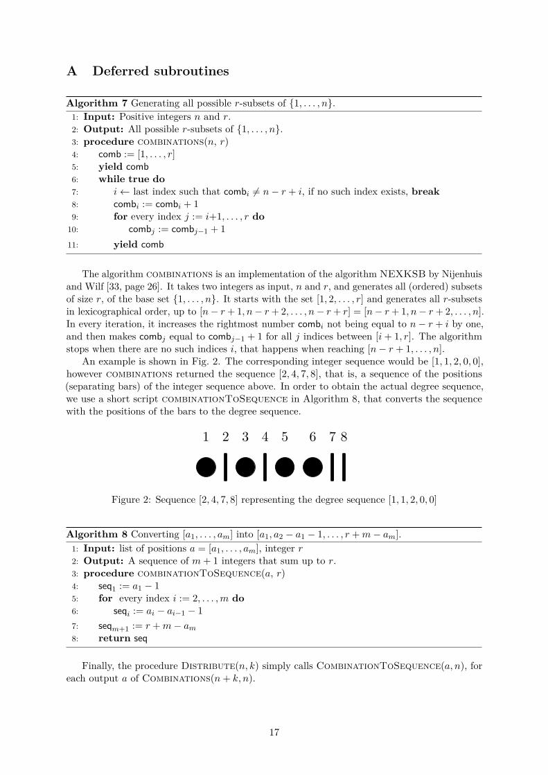
An example is shown in Fig. 2. The corresponding integer sequence would be [1, 1, 2, 0, 0],however combinations returned the sequence [2, 4, 7, 8], that is, a sequence of the positions(separating bars) of the integer sequence above. In order to obtain the actual degree sequence,we use a short script combinationToSequence in Algorithm 8, that converts the sequencewith the positions of the bars to the degree sequence.

1 2 3 4 5 6 7 8

Figure 2: Sequence [2, 4, 7, 8] representing the degree sequence [1, 1, 2, 0, 0]

Algorithm 8 Converting [a1, . . . , am] into [a1, a2 − a1 − 1, . . . , r +m− am].1: Input: list of positions a = [a1, . . . , am], integer r2: Output: A sequence of m+ 1 integers that sum up to r.3: procedure combinationToSequence(a, r)4: seq1 := a1 − 15: for every index i := 2, . . . ,m do6: seqi := ai − ai−1 − 17: seqm+1 := r +m− am

8: return seq

Finally, the procedure Distribute(n, k) simply calls CombinationToSequence(a, n), foreach output a of Combinations(n+ k, n).

17