A Theoretical High Rate Analysis of Causal versus … A Theoretical High Rate Analysis of Causal versus Unitary On-line Transform Coding† David L. Mary Aryabhatta Research Institute

1

A Theoretical High Rate Analysis

of Causal versus Unitary

On-line Transform Coding†

David L. Mary

Aryabhatta Research Institute ofObservational Sciences

Manora Peak, Nainital-263 129Uttaranchal, INDIA

Tel: 9105942-233727, extension: 228Fax: 9105942-235136

email: [email protected]

and Dirk T.M. Slock *

EURECOM InstituteMobile Communications Department

2229 route des Cretes, B.P. 19306904 Sophia Antipolis Cdx, FRANCE

Tel: +33 4 9300 2606Fax: +33 4 9300 2627

email: [email protected]

Submitted to the IEEE Transactions on Signal Processing

EDICS: SP 3-CODC

Abstract

Backward adaptive or “on-line” transform coding (TC) of Gaussian sources is investigated. We compare

in this context the Karhunen-Loeve Transform (KLT, unitary approach) to the Causal Transform (CT, causal

approach). When the covariance matrixRx of the source is used in the TC scheme, KLT and CT present similar

coding gains at high rates [1], [2], [3]. The aim of this studyis to model analytically the behavior of these two

coding structures when the ideal TC scheme gets perturbed, that is, when only a perturbed valueRx + ∆R

is known at the encoder. In the on-line TC schemes consideredhere, this estimate is used to compute both

the transform and the bit assignment.∆R is caused by two noise sources : estimation noise (finite set of

available data at the encoder) and quantization noise (quantized data at the decoder). Furthermore, not only the

transformation itself gets perturbed, but also the bit assignment. In this framework, theoretical expressions for

the coding gains in both the unitary and the causal cases are derived under high rate assumption.

†Eurecom’s research is partially supported by its industrial partners: Ascom, Swisscom, Thales Communications, STMicroelectronics, CEGETEL, France Telecom, Bouygues T´elecom, Hitachi Europe Ltd., and Texas Instruments. This workwas also supported in part by the french RNRT project COBASCA.

2

I. INTRODUCTION

A. Karhunen-Loeve and Causal Transforms in classical TC

In the classical transform coding (TC) framework (high rate, optimal bit assignment [4], [5]) the

Karhunen-Loeve transform (KLT) has become a benchmark, since it has been proved optimal for Gaus-

sian sources1 [9], [10], [11], [12]. A transform is optimal in TC if the distortion between original and

quantized data (usually the Mean Squared Error, MSE) is minimized for a given source and a given

bitrate [4], [5].

Following initial work [13], others have demonstrated theoretically [13], [14], [1], [15], [16] and nu-

merically [2] that the CT performs as well as the KLT for high bitrates (see Sec II for a quick overview

of the CT). The causal transform being moreover less computationnally expensive than the KLT, this

makes it very attractive for TC.

B. Backward Adaptive TC schemes

Classical analyses of TC (seee.g. [4], [5] and the references above) assume that the TC coding

parameters (bit assignment and transform) are available atthe encoder and decoder side. Equivalently,

the covariance matrix of the data, from which the parameterscan be computed, is assumed known at

both sides of the coder. Most of the time however, TC schemes deal with non- or locally- stationary

signals. In this case, sending the updates of the signal-dependent transformation and bit assignment

as side information may cause a considerable overhead for the overall bitrate. Hence, one can seek to

adapt these parameters on the basis of the data available at the decoder only. This backward adaptive

framework may be related to the general problem ofuniversal lossy quantization. Universality is

meant here2 as the ability of a system which has noa priori knowledge about the source, to achieve

the same rate-distortion performance as a system designed with that knowledge. Very few works have

investigated the feasibility of universal transform codesin the literature. Some techniques have been

proposed [18], [19] which rely on so-calledtwo-stagescodes: the first stage codes the identity of the

code that will be used to code the data; the second stage codesthe data with the previously chosen code.

Using one method [19] a pair (KLT; bit assignment) is chosen among a codebook of transformations

1For non Gaussian sources, different transforms may yield better compression results, seee.g. [6], [7], [8].2Different kind of universality for lossy coding, or coding with a fidelity criterion, are defined in [17].

3

and bit assignment pairs; the index of the chosen pair is sentas side-information to the decoder. This

type of technique is universal in the sense that it allows oneto code with the best transform and bit

assignment any source among a particular class. The methodsinvestigated in the present work are

different in the sense that they do not rely on “universal codebooks” of any kind. Instead of choosing

among several precomputed transforms and bit assignments,we wish the encoder and the decoder to

compute these parameters using previously decoded data only. This technique is computationally more

expensive, but does not require any side-information. The approach of the proposed analysis is similar

to that of [12], where backward adaptivity of the KLT is considered, using equal step size quantizers.

It is proved in these works that such systems may produce the same coding performances than TC

systems designed with the a priori knowledge ofRx when the numberK of available quantized vectors

becomes infinite. In the present works we propose to model andcompare the coding performances as a

functions ofK for the KLT and the CT, when both the transform and the bit assignment are backward

adaptive.

C. Formulation of the problem

Let us state more precisely the terms of the proposed evaluations. The backward adaptive systems

considered here require that neither the transformation nor the parameters of the bit assignment be

transmitted to the decoder. For the purpose of our analysis,we shall assume that the signal is a locally

stationary Gaussian vectorial signalsx with covariance matrixRx. Each source vectorxk3

= [x1,k x2,k · · · xN,k]t may seen as the sample of a vector signal, whose componentsxi,k are the

samples ofN scalar signals{xi}, i = 1, · · · ,N , taken at timek. The components of the corresponding

transform vectoryk

form a set of transform coefficients which are independentlyquantized using scalar

quantizers.

In the classical TC framework, the KLT (denoted byV ) or the CT (denoted byL) are computed so that

V RxV t, or LRxLt is diagonal. LetRy denote the covariance matrix of the transformed signals. The

variancesσ2yi

of the transform signals are(Ry)ii, where(.)ii denotes theith diagonal element of(.). The

number of bitsbi optimally allocated to each transform component isbi = b+ 12 log2

σ2yi

(QN

i=1σ2

yi)

1

N

. This

3Vectors will be denoted by underlined lowercase letters, and matrices by uppercase letters. The notationLi,j denotes the

element on theith row andjth column ofL, and superscriptt stands for transposition.

4

bit assignment algorithm is optimal in the sense that for a given set of{σ2yi} and a given per component

bitrate b, the distortion is minimized [5]. This yields the same distortion E (yi − yqi )

2 = E yi2 on

each component. The per component distortion may further may be expressed asE y2 = c 2−2biσ2yi

,

wherec is the quantizer performance factor w.r.t. the source [4]. When no transform is used (or

equivalently, the Identity transform) the distortion becomes 1N E ‖y‖2

I = c2−2b(det diag{Rx})1/N ,

where diag{a} represent the diagonal matrix with diagonala. For the KLT, the distortion becomes

1N E ‖y‖2

V = c2−2b det{Rx}1/N . In the above distortions, the subscriptsI andV refer to the transform.

[4], [5]). The corresponding coding gain for KLT is then

G0 =E ‖y‖2

I

E ‖y‖2V

=

(det{diagRx}

detRx

) 1

N

. (1)

The backward adaptive TC systems considered here can only rely on the previously decoded data.

These schemes are thus based onRx = Rx + ∆R instead ofRx, whereRx is an estimate ofRx

available at both the encoder and the decoder. Hence the transformations (V for the KLT andL for the

CT) will be such thatV RxV t or LRxLt is diagonal. LetT denote eitherV or L. The per component

distortion will be proportional to the variances of the signals transformed by means ofT , sayσ′2yi

.

Regarding the bit assignment, the bitsbi should be attributed on the basis of estimates of the variances

available at both encoder and decoder also. With the notations above, these variance estimates are

(T RxT )ii, which yields

bi = b +1

2log2

(T RxTt)ii

(∏N

i=1(T RxT t)ii)1

N

. (2)

For most of transformations used in TC, the distortion in thetransform domainE ‖y‖2 and in the signal

domainE ‖x‖2 is the same. This property is sometimes referred to as “UnityNoise Gain Property” [1].

This is indeed true for orthogonal transforms (KLT, DCT, etc...) and for the causal transform [1], [2].

We obtain therefore the following measure of distortion fora system using a transformationT based

on Rx :

E ‖y‖2bT = E

N∑

i=1

c2−2bbiσ′2yi

= E

N∑

i=1

c2

−2[b +1

2log2

(T RxT t)ii

(∏N

i=1(T RxT t)ii)1

N

]

σ′2yi

. (3)

5

where the expectationE is w.r.t. ∆R in case it is non-deterministic4.

D. High rate assumptions

Several assumptions are implicitly or not made by the above description. Firstly, we assume a Gaus-

sian source model. Secondly, the rate must be sufficiently high. The bit assignment mechanism (2)

neglects the fact thatbi can be non integer and negative. This would happen for low values of the aver-

age bitrate budgetb, or even at higher values ofb, for low values of some variancesσ′2yi

. Thirdly, the

expression (3) assumes that the quantizers’ operational distortion-rate laws are of the formc2−2biσ2yi

.

This assumes, besides high rates (independence ofc w.r.t. bi) and significance of all the transform

signals (they are assigned nonzerobi), that these transform signals belong to the family of Gaussian

probability density functions (p.d.f.s). For jointly Gaussian scalar sourcesxi composing a vectorial

sourcex, this assumption is clearly true for the transform signals obtained by means of a KLT. In

the case of a causal transform however, this is not rigorously true, because the prediction residuals

{yi}, i = 2 · · ·N , contain a quantized component through the closed loop prediction (see [2]). At

high rates however, this perturbation is small and the shapes of the p.d.f. of the{yi}, i = 2 · · ·N , are

accurately approximated by Gaussian p.d.f. (see [20]). Additionally, we shall assume that the effects

of quantization are to introduce on the data an uncorrelatedwhite noise with variancec2−2bbiσ′2yi

which

is a customary model in high rate TC, seee.g. [21], [1]. Finally, for estimation noise, the vectors to

be coded will be assumed independent and identically distributed (i.i.d.). This may be the case if the

sampling period of the scalar signals is high in comparison with their typical correlation time.

Hence, on the one hand, the proposed analysis (3) is indeed a modelization in the sense that high rate,

Gaussian sources, etc ..., may not be verified in practice by any TC system. Also some practical TC al-

gorithms may not provide the optimal, non integer bitrates bit assignment mentioned in (2) (e.g. greedy

algorithm, etc...). On the other hand, these assumptions are quite customary in TC, and without these

assumptions theoretical investigations of TC become very difficult.

4As in (3), the sign= will be used along the derivations though this equality is correct only asymptotically (w.r.t. the

rate); the sign≈ will be used when the original expression (3) will be replaced by an approximation based on the dominant

perturbation terms.

6

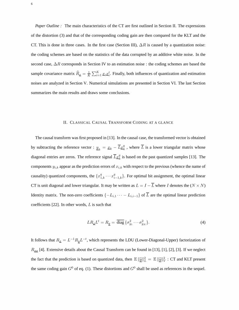
Paper Outline : The main characteristics of the CT are first outlined in Section II. The expressions

of the distortion (3) and that of the corresponding coding gain are then compared for the KLT and the

CT. This is done in three cases. In the first case (Section III), ∆R is caused by a quantization noise:

the coding schemes are based on the statistics of the data corrupted by an additive white noise. In the

second case,∆R corresponds in Section IV to an estimation noise : the codingschemes are based the

sample covariance matrixRx = 1K

∑Ki=1 xix

ti. Finally, both influences of quantization and estimation

noises are analyzed in Section V. Numerical simulations arepresented in Section VI. The last Section

summarizes the main results and draws some conclusions.

II. CLASSICAL CAUSAL TRANSFORM CODING AT A GLANCE

The causal transform was first proposed in [13]. In the causalcase, the transformed vector is obtained

by subtracting the reference vector :yk

= xk − Lxqk , whereL is a lower triangular matrix whose

diagonal entries are zeros. The reference signalLxqk is based on the past quantized samples [13]. The

componentsyi,k appear as the prediction errors ofxi,k with respect to the previous (whence the name of

causality) quantized components, the{xq1,k · · · x

qi−1,k}. For optimal bit assignment, the optimal linear

CT is unit diagonal and lower triangular. It may be written asL = I −L whereI denotes the (N ×N )

Identity matrix. The non-zero coefficients{−Li,1 · · · − Li,i−1} of L are the optimal linear prediction

coefficients [22]. In other words,L is such that

LRxLt = Ry = diag{σ2

y1· · · σ2

yN}. (4)

It follows thatRx = L−1RyL−t, which represents the LDU (Lower-Diagonal-Upper) factorization of

Rxx [4]. Extensive details about the Causal Transform can be found in [13], [1], [2], [3]. If we neglect

the fact that the prediction is based on quantized data, thenE ‖y‖2L = E ‖y‖2

V : CT and KLT present

the same coding gainG0 of eq. (1). These distortions andG0 shall be used as references in the sequel.

7

III. QUANTIZATION EFFECTS ON THECODING GAINS

In this case, transformations and bit assignment are computed using quantized data . The statistics

of the quantized data is assumed to be perfectly known in thissection. In other words, we assume that

an infinite number of quantized vectorsxqi is available at the decoder, so thatRxqxq is known.

Under the assumptions discussed in Sec. I-D,∆R = Exxt = σ2qI, whereσ2

q denotes the variance of

the quantization noise. Thus, the distortion (3) becomes

E ‖y‖2bT ,q

=

N∑

i=1

c2

−2[b +1

2log2

(TRxq T t)ii

(∏N

i=1(TRxq T t)ii)1

N

]

σ′2yi

, (5)

whereT refers to the transformation, andq refers to quantization. Expression (5) may now be evaluated

for T = I, T = V andT = L.

A. Identity Transformation

In this case, the number of bits attributed to the quantizerQi is

bi = b +1

2log2

(Rxq)ii

(∏N

i=1(Rxq)ii)1

N

, (6)

and the varianceσ′2yi

are indeed(Rx)ii. The distortion (5), whereT is replaced byI andσ′2yi

by (Rx)ii,

becomes

E ‖y‖2I,q =

N∑

i=1

c2−2r(det diagRxq

) 1

N(Rx)ii(Rxq)ii

, (7)

where diagA denotes the diagonal matrix with same diagonal asA. This leads to5

E ‖y‖2I,q = E ‖y‖2

I1N (det(I + σ2

q ( diagRx)−1))1

N tr {(I + σ2

q ( diagRx)−1)−1

}. (8)

The distortion is increased (w.r.t. a scheme based onRx) because the bits allocated on the basis of the

variances of the quantized signals are not the optimal ones.An approximation of (8) up to the second

order of the perturbations gives

E ‖y‖2I,q = c2−2r(det diag{Rx})

1/N

(ΠN

i=1(σ2

q

(Rx)ii))1/N

N∑

i=1

(1 +1

(Rx)ii

)−1

≈ E ‖y‖2I

1 +

σ4q

N2 (N−12

N∑

i=1

1

(Rx)2ii−

N∑

i=1

∑

j>i

1

(Rx)ii(Rx)jj)

.

(9)

5The calculations for the present and the following subsections are omitted for lack of space but can be found in [3].

8

The perturbation effect w.r.t. the ideal case is only causedby the perturbation upon the bit assignment.

These perturbation terms are of the form(σ2

q

(Rx)ii)2. High rate means that the quantization noise vari-

ance is small in comparison with that of the signal components. Hence we see from eq. (9) that this

perturbation is a second order term.

B. KLT

As observed in [12] also, ifV denotes a KLT ofRx, thenV (Rx + σ2qI)V t = Λ + σ2

qI = Λq, and

V is also a KLT ofRx + σ2qI. Thus, the perturbation termσ2

qI on Rx does not change the backward

adapted transformation:V = V . The variances of the transformed signals remain unchanged: σ′2yi

=

(V RxVt)ii = λi. However, the variance estimates at the decoder are(V RxqV t)ii = λi + σ2

q . These

variances are used to assign the bitsbi. These are computed as in eq. (2), whereV replacesT andRxq

replacesRx. The actual distortion becomes

E ‖y‖2V,q =

N∑

i=1

c2

−2[b +1

2log2

(V RxqV t)ii

(∏N

i=1(V RxqV t)ii)1

N

]

(V RxV t)ii

=

N∑

i=1

c2−2r(det diag{V RxqV t}

) 1

N(V RxV t)ii(V RxqV t)ii

.(10)

SinceV RxV t andV RxqV t are diagonal, one can show that

N∑

i=1

(V RxV t)ii(V RxqV t)ii

= tr {(I + σ2

q (R−1x ))−1

} = tr {(I + σ2

q (Λ)−1)−1

}. (11)

Also,

det(Rxq

)= det

(Rx

)det(I + σ2

q (R−1x )). (12)

Finally, the distortion for the KLT with quantization noiseis

E ‖y‖2V,q = E ‖y‖2

V1N (det(I + σ2

q (Λ−1)))

1

N tr {(I + σ2

q (Λ−1))−1

}. (13)

Again, the increase in distortion comes from the perturbation occurring upon the bit assignment mech-

anism. An expression approximating this distortion may be obtained by

E ‖y‖2V,q = c2−2r(det diag{Rx})

1

N1N

(N∏

i=1

(1 +σ2

q

λi)

) 1

N N∑

i=1

(1 +

σ2q

λi

)−1

.(14)

9

By developing the product and the sum in (14), it can be checked that the terms proportional toσ2q

vanish, so that

(N∏

i=1

(1 +σ2

q

λi)

) 1

N N∑

i=1

(1 +

σ2q

λi

)−1

≈ N +N − 1

2N

∑

i

σ4q

λi−

1

N

N∑

i=1

∑

j>i

σ4q

λiλj. (15)

This leads to the following approximated distortion

E ‖y‖2V,q ≈ E ‖y‖2

V

1 +

σ4q

N2

N−1

2

N∑

i=1

1

λ2i

−N∑

i=1

∑

j>i

1

λiλj

(16)

Using (8) and (13), the corresponding expression for the coding gain in the unitary case with quantiza-

tion noise is

GV,q = G0 (det(I + σ2q ( diagRx)−1))

1

N tr {(I + σ2

q ( diagRx)−1)−1

}

(det(I + σ2q(Λ

−1)))1

N tr {(I + σ2

q (Λ−1))−1

}. (17)

With (9) and (16),GV,q can be approximated as

GV,q ≈ G0

1 +

σ4q

N2

N − 1

2

N∑

i=1

(1

(Rx)2ii−

1

(λi)2) −

N∑

i=1

∑

j>i

(1

(Rx)ii(Rx)jj−

1

λiλj)

. (18)

The perturbation effect w.r.t. the ideal case is only causedby the perturbation upon the bit assignment.

As in the case of Identity transformation, the perturbationterms in eq. (18) are second order terms of

the form(σ2

q

(Rx)ii)2 or (

σ2q

λi)2.

C. Causal Transform (CT)

In the causal case, the encoder computes a transformationL = L′ such thatL′RxqL′T = R′

y. The

causal transform corresponds to a LDU factorization ofRxq . R′

y is the diagonal matrix of the variances

used for the bit assignment (L′ andR′

y are both available to the decoder). In this case, the difference

vectory is x − L′xq. By the analysis of [2], the quantization noise is filtered bythe rows ofL′ (see

Figure 1). Note that in this caseE ‖x‖2L′,q still equalsE ‖y‖2

L′,q, sincex = xq −x = yq + L′xq −x =

yq − y = y.

Regarding the estimates of the rates, they are computed by eq. (2), whereT is replaced byL′, andRx

by Rxq . At high rates, it is shown in [2] that the actual variances ofthe signalsyi obtained by means of

10

L′ may be approximated as(L′RxqL′T − σ2

qI)ii. Using (5), the distortionE ‖y‖2L′,q is then given by

E ‖y‖2L′,q = c2

−2[b +1

2log2

(L′RxqL′T )ii

(∏N

i=1(L′RxqL

′T )ii)1

N

] N∑

i=1

(L′RxqL′T − σ2

qI)ii

≈N∑

i=1

c2−2r(det diag{L′RxqL

′T }) 1

N

(1 −

(σ2qI)ii

(L′RxqL′T )ii

).

(19)

Since the transformationL′ is unimodular6, the determinant in the previous expression equals the deter-

minant in (12). The sum in (19) may be written as tr{(I − σ2q(L

′RxqL′T )−1)} = tr {(I − σ2

qR′

y−1)}.

Thus (19) becomes

E ‖y‖2L′,q = E ‖y‖2

L

1

N(det(I + σ2

q(Λ−1)))

1

N tr {(I − σ2

q (R′−1

y ))}. (20)

The excess in distortion comes not only from the perturbation occurring on the bit assignment mech-

anism but also from the filtering of the quantization noise. Up to the first order of perturbations, we

obtain

E ‖y‖2(L′,q = c2−2r(det diag{Rx})

1

N

(N∏

i=1

(1 +σ2

q

λi)

) 1

N N∑

i=1

(1 − σ2

q

1

(R′

yy)ii

)

≈ E ‖y‖2V

[1 +

σ2q

N

N∑

i=1

(1

λi−

1

σ2yi

)],

(21)

where theσ2yi

correspond to optimal prediction error variances in absence of quantization noise.

The corresponding exact expression for the coding gain is

GL′,q = G0 (det(I + σ2q ( diag{Rx})

−1))1

N tr {(I + σ2

q( diag{Rx})−1)−1

}

(det(I + σ2q(Λ

−1)))1

N tr {(I − σ2

q (R′−1

y ))}

. (22)

Up to the first order of perturbation we get,

GL′,q ≈ G0

[1 −

σ2q

N

N∑

i=1

(1

λi−

1

σ2yi

)]. (23)

The approximated expression (23) shows that the perturbation effects of the bit assignment mechanism

(2nd order terms) are in the causal case negligible in comparison with those of the noise feedback (1st

order terms). This coding gain is similar to that obtained in[2], where only the noise feedback was

accounted for (no perturbation on the bit assignment).

An interesting consequence of (23) is that the performance of the causal TC scheme depend on the

6L being unit diagonal and lower triangular, its determinant equals the product of its diagonal elements, which is one.

11

order in which the signals{xi} get decorrelated. As shown in [2], the signalsxi should be decorrelated

by order of decreasing variance if we wantGL′,q to be maximized (see also Fig. 3 and 6 in Section

VI). In other words, in the vectorxk = [x1,k x2,k . . . xN,k]t, the componentx1 should be that of largest

variance,x2 the component with second largest variance, etc..., if we want the noise feedback to be

minimized.

IV. ESTIMATION NOISE

We analyze in this section the coding gains of a backward adaptive scheme based on an estimate of

the covariance matrixRx = 1K

∑Ki=1 xix

ti = R + ∆R, where∆R corresponds to the estimation noise.

In the following, the subscriptK refers to the estimation noise corresponding toK vectors. In this

case, one can show that∆R is a zero mean Gaussian random variable, with

E vec(∆R) (vec(∆R))t ≈2

KRx ⊗ Rx, (24)

where⊗ denotes the Kronecker product.

Using K data vectors, encoder and decoder compute a transformationT which diagonalizesRx :

T RxT = Ry. The number of bits assigned to each component is as in eq. (2),with the definition ofT

andRx above.

Now, the actual variances of the signals obtained by applying T to x are(TRxTt)ii. Note that in the

causal case,y = I−Lx = Lx, so thatR′

y = LRxLt. In the causal case, there is a qualitative difference

with the previous section, where the quantization noise wasfiltered by the predictors ofL′. Here, the

estimation noise does not perturb signals, but only transformations and bit assignments. The resulting

distortion for a sample covariance matrix based onK vectors is as in eq. (3), withσ2′yi

= (TRxT t)ii.

A. Identity Transformation

With T = I, and using a similar analysis as in the previous section, we obtain for the distortion

E ‖y‖2I,K = E c2−2r

(det diag{Rx}

) 1

N

(N∏

i=1

(1 +(∆R)ii(Rx)ii

)

) 1

N N∑

i=1

(1 +

(∆R)ii(Rx)ii

)−1

≈ E ‖y‖2I

1 + E

N−12N2

N∑

i=1

((∆R)ii(Rx)ii

)2 − E1

N2

∑

i

∑

j>i

(∆R)ii(Rx)ii

(∆R)jj(Rx)jj

(25)

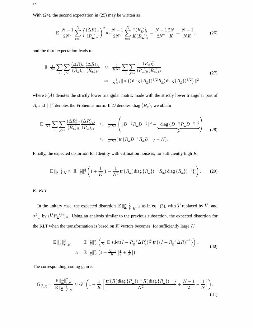
12

With (24), the second expectation in (25) may be written as

EN − 1

2N2

N∑

i=1

((∆R)ii(Rx)ii

)2

≈N − 1

2N2

N∑

i=1

2(Rx)2iiK(Rx)2ii

=N − 1

2N2

2N

K=

N − 1

NK, (26)

and the third expectation leads to

E1

N2

∑

i

∑

j>i

(∆R)ii(Rx)ii

(∆R)jj(Rx)jj

≈ 2KN2

∑

i

∑

j>i

(Rx)2ij(Rx)ii(Rx)jj

≈ 2KN2‖ .

(( diag{Rx})

1/2Rx( diag{Rx})1/2)‖2

(27)

where.(A) denotes the strictly lower triangular matrix made with the strictly lower triangular part of

A, and‖.‖2 denotes the Frobenius norm. IfD denotes diag{Rx}, we obtain

E1

N2

∑

i

∑

j>i

(∆R)ii(Rx)ii

(∆R)jj(Rx)jj

≈ 1KN2

‖D−

1

2 RxD−1

2‖2 − ‖diag{D−1

2 RxD−1

2‖2

︸ ︷︷ ︸N

≈ 1KN2 ( tr {RxD−1RxD−1} − N).

(28)

Finally, the expected distortion for Identity with estimation noise is, for sufficiently highK,

E ‖y‖2I,K ≈ E ‖y‖2

I

(1 +

1

K[1 −

1

N2tr {Rx( diag{Rx})

−1Rx( diag{Rx})−1}]

). (29)

B. KLT

In the unitary case, the expected distortionE ‖y‖2bV ,K

is as in eq. (3), withT replaced byV , and

σ2′yi

by (V RxV t)ii. Using an analysis similar to the previous subsection, the expected distortion for

the KLT when the transformation is based onK vectors becomes, for sufficiently largeK

E ‖y‖2bV ,K

= E ‖y‖2V

(1N E (det(I + R−1

x ∆R))1

N tr {(I + R−1

x ∆R)−1

})

.

≈ E ‖y‖2V

(1 + N−1

K

[12 + 1

N

]) (30)

The corresponding coding gain is

GbV ,K=

E ‖y‖2I,K

E ‖y‖2bV ,K

≈ G0

(1 −

1

K

[tr {R( diag{Rx})

−1R( diag{Rx})−1}

N2+

N − 1

2−

1

N

]).

(31)

13

C. Causal Transform (CT)

As commented in the introduction of this section, the expected distortion withL computed withRx

is

E ‖y‖2bL,K

= E

N∑

i=1

c2

−2[b +1

2log2

(LRxLt)ii

(∏N

i=1(LRxLT )ii)1

N

]

(LRxLt)ii

= E c2−2r(det LRxLt

) 1

N

N∑

i=1

(LRxLt)ii

(LRxLt)ii,

(32)

where we used a factorization similar to that used in (7). Nowby the unimodularity property ofL, we

can write the determinant in (32) as

(det LRxLt

) 1

N= det Rx = det(Rx) det(I + R−1

x ∆R), (33)

and sinceL diagonalizesRx, we can write the sum in (32) as

N∑

i=1

(LRxLt)ii

(LRxLt)ii= tr {(I + R−1

x ∆R)−1}. (34)

The perturbation terms in eq. (33) and (34) are the same in thecausal and the unitary case : the

equality of the determinants in eq. (33) comes from the unimodularity of the transformationsL and

V , and the equality of the traces in (34) comes from their decorrelating property. Hence, because

both CT and unitary KLT are decorrelating and unimodular transforms, they yield the same distortion

E ‖y‖2bL,K

= E ‖y‖2bV ,K

, as given by eq. (30). The coding gains with estimation noiseare thus equal

for KLT and CT and may be approximated by eq. (31).

V. QUANTIZATION AND ESTIMATION NOISE

This Section deals with the most general case of this study. In presence of quantization and es-

timation noises, transforms and bit assignment should be computed using a numberK of decoded

vectors, or equivalently usingRxq = 1K

K∑

i=1

xqi x

qt

i . The estimated transformT is such thatTRxq T t is

a diagonal matrix, which corresponds to the estimated variances of the transformed signals. We shall

continue denoting byσ′2yi

the actual variances of the transformed signals (obtained by applying T to

xk). The expected distortionE ‖y‖2bT ,K,q

can be computed as in eq. (3), withRx replaced byRxq (the

14

subscriptsq andK refer to the presence of quantization and estimation noise). This distortion must now

be evaluated for Identity, KL and causal transforms.

A. Identity Transformation

With T = I, and by writingRx = Rxq − σ2qI, we obtain

E ‖y‖2I,K,q = E

N∑

i=1

c2

−2[b +1

2log2

(Rxq)ii

(∏N

i=1(Rxq)ii)1

N

]

(Rxq)ii

−σ2q E

N∑

i=1

c2

−2[b +1

2log2

(Rxq)ii

(∏N

i=1(Rxq)ii)1

N

]

.

(35)

For sufficiently high resolution and largeK, the expected distortion for Identity transform with quanti-

zation and estimation noise leads to

E ‖y‖2I,K,q ≈ E ‖y‖2

I

(det(I + σ2

q ( diag{Rx})−1))1/N

×[1 + 1

K

[1 − 1

N2 tr {Rxq( diagRxq)−1Rxq( diagRxq)−1}]−

σ2q

N tr {( diagRxq)−1}].

(36)

B. KLT

In the unitary case,σ2′yi

= (V RxV t)ii. After some computation we find for the expected distortion

in the unitary case, when the transformation is based onK quantized vectors,

E ‖y‖2bV ,K,q

≈E ‖y‖2V

(det(I + σ2

q(Rx)−1)) 1

N

[1 +

N − 1

K

[1

2+

1

N

]−

σ2q

Ntr {(Rxq)−1}

], (37)

for largeK and under high resolution assumption. The corresponding expression for the coding gain is

GbV ,K,q=

E ‖y‖2I,K,q

E ‖y‖2bV ,K,q

≈ G0

(det(I + σ2

q ( diag{Rx})−1))1/N

(det(I + σ2

q (Rx)−1))1/N

×

[1 + 1

K (1 − 1N2 tr {Rxq( diag{Rxq})−1Rxq( diag{Rxq})−1}) −

σ2q

N tr {( diag{Rxq})−1}]

[1 + N−1

K (12 + 1

N ) −σ2

q

N tr {(Rxq)−1}] .

(38)

The above expression exhibit three kinds of terms : those regarding estimation noise only (throughK),

those regarding quantization noise only (throughσ2q ), and cross influence terms.

15

C. Causal Transform (CT)

In the causal case, an estimateL′ is computed fromRxq , and the actual variances areσ′2yi

=

E (L′Rxq L′T − σ2

qI)ii. Thus, when the transformation is based onK quantized vectors (for high

K and under high resolution assumption) the distortion becomes

E ‖y‖2bL′,K,q

= E

N∑

i=1

c2

−2[b +1

2log2

(L′Rxq L′T )ii

(∏N

i=1(L′Rxq L

′T )ii)1

N

]

(L′Rxq L′T − σ2

qI)ii. (39)

The above expression leads to

E ‖y‖2bL′,K,q

≈ E ‖y‖2L

(det(I + σ2

q (Rx)−1))1/N

[1 +

N − 1

K

[1

2+

1

N

]−

σ2q

Ntr {(R′

y)−1}

]. (40)

The corresponding expression for the coding gain in the causal case can then be estimated as

GbL′,K,q=

E ‖x‖2I,K,q

E ‖y‖2bL′,K,q

≈ G0

(det(I + σ2

q( diag{Rx})−1))1/N

(det(I + σ2

q (Rx)−1))1/N

×

[1 + 1

K

[1 − 1

N2 tr {Rxq( diag{Rxq})−1Rxq( diag{Rxq})−1}]−

σ2q

N tr {( diag{Rxq})−1}]

[1 + N−1

K

[12 + 1

N

]−

σ2q

N tr {(L′RxqL′T )−1}

] .

(41)

Again, perturbation terms regarding the influence of quantization, estimation noise, and both can be

identified.

It can be checked that the expressions (41) and (38) tend to (17) and (22) respectively asK → ∞, and

both to (31) asσ2q → 0. This means indeed that asK → ∞, the estimation noise vanishes, and we

face a quantization noise problem only, which leads to the results of Sec. III. Asσ2q → 0 also, only

estimation noise remains, which leads to the results of Sec.IV.

16

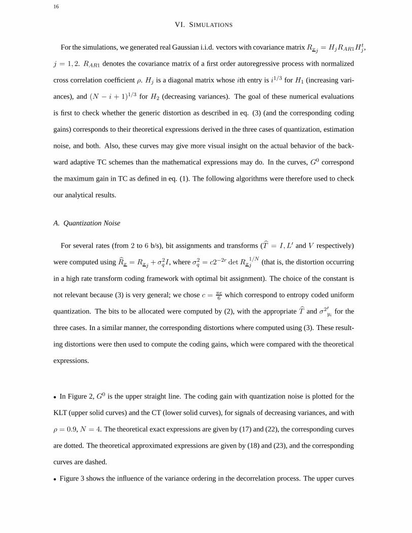
VI. SIMULATIONS

For the simulations, we generated real Gaussian i.i.d. vectors with covariance matrixRxj = HjRAR1Htj ,

j = 1, 2. RAR1 denotes the covariance matrix of a first order autoregressive process with normalized

cross correlation coefficientρ. Hj is a diagonal matrix whoseith entry isi1/3 for H1 (increasing vari-

ances), and(N − i + 1)1/3 for H2 (decreasing variances). The goal of these numerical evaluations

is first to check whether the generic distortion as describedin eq. (3) (and the corresponding coding

gains) corresponds to their theoretical expressions derived in the three cases of quantization, estimation

noise, and both. Also, these curves may give more visual insight on the actual behavior of the back-

ward adaptive TC schemes than the mathematical expressionsmay do. In the curves,G0 correspond

the maximum gain in TC as defined in eq. (1). The following algorithms were therefore used to check

our analytical results.

A. Quantization Noise

For several rates (from2 to 6 b/s), bit assignments and transforms (T = I, L′ andV respectively)

were computed usingRx = Rxj + σ2qI, whereσ2

q = c2−2r det Rx1/Nj (that is, the distortion occurring

in a high rate transform coding framework with optimal bit assignment). The choice of the constant is

not relevant because (3) is very general; we chosec = πe6 which correspond to entropy coded uniform

quantization. The bits to be allocated were computed by (2),with the appropriateT andσ2′yi

for the

three cases. In a similar manner, the corresponding distortions where computed using (3). These result-

ing distortions were then used to compute the coding gains, which were compared with the theoretical

expressions.

• In Figure 2,G0 is the upper straight line. The coding gain with quantization noise is plotted for the

KLT (upper solid curves) and the CT (lower solid curves), forsignals of decreasing variances, and with

ρ = 0.9, N = 4. The theoretical exact expressions are given by (17) and (22), the corresponding curves

are dotted. The theoretical approximated expressions are given by (18) and (23), and the corresponding

curves are dashed.

• Figure 3 shows the influence of the variance ordering in the decorrelation process. The upper curves

17

(solid: observed and dots: theoretical) depict the gain obtained with the CT by decorrelating the signals

by decreasing order of variance (Rx2), and the lower curves (solid and diamond) by increasing order

(Rx1). The theoretical expression is eq. (22).

From these Figures, it is checked that the expressions (17) and (22) are actually exact. From Fig.

2, approximated expressions (18) and (23) match their exactcounterparts as the rate increases. The

performances of the CT are slightly inferior to those of the KLT (from a few percents) and vanishes

at high rates. From Fig. 3, it appears that processing the signals by order of decreasing variance

maximizes the coding gain, as discussed in Sec. III-C.

B. Estimation Noise

In this case, estimates of the covariance matrix of the data were computed usingK vectors by

1K

∑Ki=1 xix

ti, K = N,N+1, · · · , 103. For each estimateRx, the transformsT = V , L were computed

so thatT RxT t is diagonal, and the bit assignments were computed using estimates of the variances

(T RxT t)ii. In order to evaluate the expected distortion (3), the sum in(3) was considered as a random

variable, whose expectation was evaluated by Monte Carlo simulations. This was done for the Identity

transform, in the causal and in the unitary case. The coding gains in presence of estimation noise are

compared forN = 4 andρ = 0.9. The ratio of the corresponding distortions are the “ObservedG” in

Figure 4. The corresponding theoretical expression (“Theoretical G”) is given by (31) (it should be the

same for the KLT and CT because both transforms are decorrelating and unimodular).G0 is the upper

straight line.

As expected, there is no difference between the unitary and the causal case. Our calculations assume

small perturbations (largeK). It can be observed that the model matches the actual codinggain after a

few tens of vectors. Backward adaptive systems yield similar performances as systems designed with

the knowledge ofRx after a few hundreds of decoded vectors. Note also that it is always useful to use

backward adaptive TC schemes (the coding gain is superior to1 for K > N + 1).

C. Quantization and Estimation Noise

In this case, the quantized vectors were obtained for each rate r by adding to the sets of i.i.d. Gaus-

sian vectors uncorrelated white noise vectors with covariance matrixσ2qI = c2−2r(det Rx)

1

N I. For

18

each set ofK quantized vectors, an estimate of the covariance matrix of the data was computed by

1K

∑Ki=1 x

qi x

qit, K = N,N + 1, · · · , 103. Again, for each estimateRxq , the transformsT = V , L

were computed so thatTRxq T t is diagonal, and the bit assignments were computed using estimates

of the variances(T Rxq T t)ii. In order to evaluate the expected distortion for the three transformations,

the sum was considered as a random variable, whose expectation was evaluated by Monte Carlo sim-

ulations. The ratio of the corresponding distortions are the “Observed Gains” of the following figures.

The theoretical gains are given by (38) for KLT and (41) for LDU.

• The coding gains in presence of estimation and quantizationnoise are compared for KLT and CT

(signals of decreasing variances) in Figure 5 forN = 4, ρ = 0.9 and a rate of3 bits per sample. Upper

straight line isG0. The upper solid line curve is the theoretical coding gain for KLT, and the lower

solid line curve the theoretical coding gain for CT. The upper dashed curve is the observed coding gain

for KLT, and the lower dashed curve the observed coding gain for CT.

The observed behaviors of the transformation are relatively well matched by the theoretically predicted

ones asK amounts to a few tens. AsK amounts to a few hundreds, the performances of on-line systems

approach those of systems designed with the optimal transforms and bit assignment. The performances

of the CT are slightly inferior to those of the KLT. This difference vanishes at high rates (cf Fig. 2). In

Fig. 5, the coding gains toward which both the KLT and the CT system converge can be read from Fig.

3, with r = 3 b/s.

• The influence of the ordering of the signals for the same parameters as above is plotted in Figure 6.

In the limit of largeK, the actual gains converge to the results obtained in the case where quantiza-

tion noise only is considered (the estimation noise vanishes). The proposed model matches the actual

convergence behaviors in the causal and unitary cases aftera few tens of decoded vectors. Finally,

decorrelating the signals by order of decreasing variance appears the best strategy.

VII. SUMMARY AND CONCLUSIONS

We proposed an analytical model for the performances of causal and unitary on-line TC schemes.

We described the effects of backward adaptation as perturbation effects : backward adaptation impacts

the ideal high rate TC framework by perturbing both the transforms’ design and the bit assignment

19

mechanism.

It appears that as quantization noise only is considered, only the bit assignment mechanism is perturbed

for the KLT (2nd order perturbation term), whereas the CT suffers additionally from quantization noise

feedback (1st order term). As one accounts for estimation noise only, both transforms present the same

performances because they are both decorrelating and unimodular. As both types of perturbations are

accounted for, the CT remains slightly inferior from a rate-distortion point of view to its unitary coun-

terpart because of the quantization noise feedback. This drawback vanishes at high rates. It can be

minimized if the signals get decorrelated by order of decreasing variances.

As K amounts to a few hundreds, the performances of on-line TC systems approach those of systems

designed with the optimal transforms and bit assignment. The on-line TC systems modeled by eq. (2)

and (3) are advantageous w.r.t. a system using no transform for values ofK larger than≈ N + 1

vectors.

The results of simulation show that the analytical description of the considered systems is fairly ac-

curate. We provided exact expressions for the coding gains as far as the quantization noise only is

concerned. When estimation noise is accounted for, the proposed analysis reliably estimates the distor-

tions and the corresponding coding gains after a few tens of decoded vectors.

As a follow-up of these works, we are currently investigating systems using different bit assignment

mechanisms than that assumed in eq. (2).

20

REFERENCES

[1] S.-M. Phoong and Y.-P. Lin, “Prediction-based lower triangular transform,”IEEE trans. on Sig. Proc., July 2000.

[2] D. Mary and D.T.M. Slock, “On quantization noise feedback in causal tranform coding,” 2004, Submitted to IEEE

Trans. on Signal Processing.

[3] D. Mary, Causal Lossy and Lossless Coding of Vectorial Signals, Ph.D. thesis, ENST, Paris, March 2003.

[4] N.S. Jayant and P. Noll,Digital Coding of Waveforms, Prentice Hall, 1984.

[5] A. Gersho and R.M. Gray,Vector quantization and signal compression, Kluwer Academic, 1992.

[6] V.K. Goyal, “Theoretical foundations of transform coding,” IEEE Signal Processing Magazine, vol. 18, no. 5, pp. 9–21,

Sept. 2001.

[7] M. Effros, H. Feng, and K. Zeger, “Suboptimality of Karhunen-Loeve transform for transform coding,”IEEE Trans. on

Inf. Th., pp. 1605–1619, August 2004.

[8] M. Effros, “Rate-distortion bounds for fixed- and variable-rate multiresolution sources codes,” Submitted to IEEE

Trans. on Inf. Theory on March 26, 1998.

[9] K. Karhunen, “Uber lineare Methoden in der Wahrscheinlichkeitsrechnung,”Ann. Acad. Sci. Fenn., Ser. A1,: Math.-

Phys., vol. 37, pp. 3–79, 1947.

[10] M. Loeve, Processus stochastiques et mouvements Browniens, chapter : Fonctions aleatoires de second ordre, P. Levy,

Ed. Paris, France : Gauthier-Villars, 1948.

[11] H. Hotelling, “Analysis of a complex of statistical variables into principal components,”J. Educ. Psychology, vol. 24,

pp. 417–441, 498–520, 1933.

[12] V. Goyal, J. Zhuang, and M. Vetterli, “Transform codingwith backward adaptive updates,”IEEE Trans. on Inf. Th.,

vol. 46, no. 4, July 2000.

[13] Habibi A. and Hershell R.S., “A unified framework of differential pulse-code modulation (DPCM and transform coding

systems,”IEEE Trans. on Com., pp. 692–696, May 1974.

[14] S.M. Phoong and Y.P. Lin, “PLT versus KLT,” inIEEE Int. Symp. Circ. Syst., May 1999.

[15] D. Mary and D. T. M. Slock, “Codage DPCM vectoriel et application au codage de la parole en bande elargie,” in

CORESA 2000, Poitiers, France, October 2000.

[16] F. Lahouti and A.K. Khandani, “Sequential vector decorrelation technique,” Tech. Rep., Univ. of Waterloo, 2001.

[17] D. L. Neuhoff, R. M. Gray, and L. D. Davisson, “Fixed rateuniversal block source coding with a fidelity criterion,”

IEEE Trans. Inf. Theory, vol. IT-21, pp. 511–523, Sept. 1975.

[18] P. A. Chou, M. Effros, and R.M. Gray, “A vector quantization approach to universal noiseless coding and quantization,”

IEEE Trans. on Inf. Theory, vol. 42, no. 4, pp. 1109–1138, July 1996.

[19] M. Effros and P. A. Chou, “Weighted universal transformcoding: Universal image compression with the Karhunen-

Love transform,” inProc. Int. Conf. Image Processing, Oct. 1995, vol. II, pp. 61–64.

[20] D. Mary and D. T. M. Slock, “On the suboptimality of orthogonal transforms for single- or multi-stage lossless transform

21

coding,” inDCC, 2003.

[21] P. P. Vaidyanathan,Multirate Systems and Filter Banks, Prentice Hall, Englewood Cliffs, NJ, 1993.

[22] J. Makhoul, “Linear prediction : a tutorial review,”Proc. IEEE, vol. 63, pp. 561–580, April 1975.

List of Figures

Fig. 1. Backward adaptation of the causal transform with quantization noise.L = I − L = I − L′ is

used to compute the reference vectorL′xqk.

Fig. 2. Quantization noise : Coding Gainsvsrate in bit/sample. quantizers).

Fig. 3. Quantization noise : Influence of the ordering of the signalsxi.

Fig. 4. Estimation noise : Coding Gains for KLT and CT with estimation noise.

Fig. 5. Estimation and quantization noise : Coding Gains for KLT andCT ρ = 0.9. The rate is3 b/s

andN = 4.

Fig. 6. Estimation and quantization noise. Influence of the ordering of the subsignals : Compared cod-

ing gains for CT. The rate is3 b/s andN = 4.

+

+

+

−

−

−

y2,k

...

......

+

+

+

.........

...

+

+

+

x1,k

x2,k

xN,k

y1,k

Q1

Q2

QN

yN,k

yq1,k

yq2,k

yqN,k

xq1,k

xq2,k

xqN,k

L′

Fig. 1.

2 2.5 3 3.5 4 4.5 5 5.5 63.2

3.25

3.3

3.35

3.4 CT

3.45 KLT

3.5

Rate (bit per sample)

Cod

ing

Gai

n

G0 Observed G: CT Observed G: KLT Theoretical G CT : exact Theoretical G KLT : exact Theoretical G CT : approx.Theoretical G KLT : approx.

Fig. 2.

2 2.5 3 3.5 4 4.5 5 5.5 63.15

3.2

3.25

3.3

3.35

3.4

3.45

3.5

3.55

Rate (bit per sample)

Cod

ing

Gai

n ov

er Id

entit

y

Theoretical G : DecreasingObserved G : DecreasingTheoretical G : IncreasingObserved G : Increasing

Fig. 3.

101

102

103

0

0.5

1

1.5

2

2.5

3

3.5

Number of Quantized Vectors K

Gai

n ov

er Id

entit

y

G0 Observed G: CTObserved G: KLTTheoretical G

Fig. 4.

101

102

103

0

0.5

1

1.5

2

2.5

3

3.5

Gai

n ov

er Id

entit

y

Number of Quantized Vectors

G0 Theoretical Gain: CTObserved Gain : CT Theoretical Gain: KLTObserved Gain : KLT

Fig. 5.

101

102

103

0

0.5

1

1.5

2

2.5

3

3.5

G0 Theoretical Gain: CT Decreasing Observed Gain : CT Decreasing Theoretical Gain: CT Increasing Observed Gain : CT Increasing

Fig. 6.