A test of the rational expectations hypothesis using data from a natural experiment

A Test of the Rational Expectations Hypothesis using data

from a Natural Experiment

by

Anna Conte, Peter G. Moffatt♠, Fabrizio Botti, Daniela T. Di Cagno, and Carlo D’Ippoliti

ABSTRACT

Data on contestants’ choices in Italian Game Show Affari Tuoi are analysed in a way that sepa-rates the effect of risk attitude from that of beliefs concerning the amount of money that will be offered to contestants in future rounds. The importance of belief-formation is confirmed by the estimation of a mixture model which establishes that the vast majority of contestants are for-ward-looking as opposed to myopic. The most important issue addressed in the paper is what belief function is actually being used by contestants. This function is estimated in an uncon-strained way as a component of the choice model, which is estimated using maximum simulated likelihood. Separate identification of the belief function and preferences is possible by virtue of the fact that at a certain stage of the game, beliefs are not relevant, and risk attitude is the sole determinant of choice. The rational expectations hypothesis is tested by comparing the esti-mated belief function with the “true” offer function which is estimated using data on offers ac-tually made to contestants. We find that there is a significant difference between these two functions, and hence we reject the rational expectations hypothesis. However, when a simpler “rule-of-thumb” structure is assumed for the belief function, we find a correspondence to the function obtained from data on actual offers. Our overall conclusion is that contestants are ra-tional to the extent that they make use of all available relevant information, but are not fully ra-tional because they are not processing the information in an optimal way. The importance of allowing the choice data to convey the belief function without prejudice is emphasised. JEL Codes: C15; C23; C25; D81. Key words and phrases: Beliefs; Discrete choice models; Method of simulated likelihood; Natural Ex-

periments; rational expectations; risky choice. LUISS Guido Carli, University of Rome I “La Sapienza” and University of Rome II “Tor Vergata”; e-

mail: [email protected] ♠ School of Economics, University of East Anglia: [email protected] (Corresponding Author) LUISS Guido Carli; e-mail: [email protected] LUISS Guido Carli; e-mail: [email protected] LUISS Guido Carli and University of Rome “La Sapienza”: [email protected]

1

A Test of the Rational Expectations Hypothesis using data from a Natural Experiment

1. Introduction When an individual is faced with a choice problem under risk, that individual’s risk attitude is the principal determinant of their choice. However, this assumes that the payoff from the choice is instantaneous. If the payoff is made at some future date, and the eventual payoff is dependent on the state of the world at that future date, or on some intervention by others, then the individ-ual’s beliefs of what will pertain at that future date must enter the decision making process. Obvious examples are found in economics: schooling decisions depend on individuals’ beliefs about the structure of the labour market that will pertain several years in the future; firms base their investment and production plans on beliefs about the future evolution of consumer prefer-ences. Researchers analysing such decisions clearly cannot rely solely on choice data, because any ob-served choice is usually compatible with many different combinations of risk attitudes and be-liefs. This is a problem that is frequently encountered in experimental economics, although not all researchers appear to recognise it or to pay due attention to it. One notable exception is Manski (2002), who analyses the problem in the context of an ultima-tum game. He emphasises that the proposer’s decision depends on their subjective probability distribution of the respondent’s possible reactions, and that knowledge of the observed decision alone is insufficient to identify the proposer’s decision-making process. In contexts such as this, researchers have tended to appeal to rational expectations theory, and to assume that agents form the same beliefs as would a researcher with access to econometric estimation facilities. This, of course, places structure on agent’s beliefs, allowing the researcher to isolate risk atti-tudes (henceforth “preferences”). However, although many tests of the rational expectations hypothesis appear in the macroeconomics literature (see Attfield et al., 1991), there is little evi-dence of whether agents behave according to the rational expectations hypothesis in microeco-nomic contexts. An alternative approach, reviewed by Manski (2004), is to ask individuals directly about their beliefs. Bellemare et al. (2005) follow the same approach, again in the context of an ultimatum game. They find that a model estimated with this information on beliefs incorporated, has higher predictive power than a model based on the assumption of rational expectations. How-ever, belief elicitation can itself cause problems: Rutström and Wilcox (2006), in an experiment on the repeated matching pennies game, find that agents tend to alter their strategies when asked to state their beliefs about opponents’ behaviour. In recent years, the analysis of data from television game shows has become a popular means of analysing individuals’ behaviour under risk. It is obvious why researchers favour this sort of data. Game shows provide a good natural context in which contestants face well-defined deci-sion problems in a ceteris paribus environment. Furthermore, it cannot be denied that contest-ants have salient incentives, allowing studies using such data to overcome both the Harrison and List (2004) and the Rabin (2000) critiques.1 One game show that scores particularly highly on these criteria is the Italian show Affari Tuoi, data from which is analysed in this paper. This game is played in many different countries under different names and with slightly different rules. Researchers seem to be in agreement on the usefulness of the resulting data: Bombardini and Trebbi (2007) assert that Affari Tuoi “presents several features that we would have chosen,

1 See, among the others, Friend and Blume (1975), Gertner (1993), Metrick (1995), Beetma and Shotman (2001) and Hartley et al. (2005) for an analysis of individual risk attitude through TV games.

2

were we to design such an experiment”; Post et al (2007) describe the Dutch version of the same game as having “such desirable features that it almost appears to be designed to be an econom-ics experiment rather than a TV show”. The rules of Affari Tuoi will be explained in detail in Section 2. For the time being, let us sim-ply recognise that the contestant faces a sequence of choice problems, in which the choice is be-tween an uncertain lottery, and a certain amount offered by the “Banker”, and that if the Banker’s offer is accepted, the game ends. Many researchers have now realised that, at each stage of the game, a typical contestant is not treating the choice problem as a single isolated task, but is instead forming beliefs of what will happen in future rounds, and using these beliefs in making their decision in the current round. In particular, they are forming an expectation of what the Banker’s offer will be in future rounds, should they stay in the game. It is clear that such beliefs have the potential to influence the current decision. It is also clear that this setting bears similar features to that of the ultimatum game considered earlier, with the attendant diffi-culties in separately identifying preferences and beliefs. There has been a large volume of recent research analysing data from the various different ver-sions of this game show (see the survey of Andersen at al., 2007). Much of this research has fo-cussed on the search for the best characterisation of behaviour under risk. Typically, the as-sumption of rational expectations is implicitly adopted, whereby the inferential problem of pre-dicting the Banker’s offer is solved outside the choice model. This is done in a variety of ways, usually based on parametric characterisations (e.g., de Roos and Sarafidis (2006), Deck et al. (2006) and Mulino et al. (2006)). In this paper, we treat the formation of beliefs about the Banker’s offer as the central focus. In particular, by incorporating a predicted Banker’s offer equation into the choice model, we are able to estimate the equation that contestants actually use to form beliefs. We are then able to compare this true belief equation with the equation that would be used under the assumption of rational expectations, hence enabling a formal test of the rational expectations hypothesis. With these objectives in mind, we note that the game show has a peculiar structure: in the final round of the game, contestants’ choices unequivocally reveal information on their risk aversion (since there is no contamination from beliefs about future rounds). Without data from this round, it would be impossible to distinguish between a contestant who is very risk averse but has optimistic beliefs about future offers, and one who is risk-loving but has pessimistic beliefs of future offers. The information on risk attitude extracted from the choice made in the final round is combined with information on choices from earlier rounds in order to identify the pa-rameters of the offer function that is used by contestants in these earlier rounds. In addition to testing for rational expectations, we provide an assessment of the validity of an-other assumption that has been made in previous work: that all contestants are forward-looking. While it may seem natural for contestants to base their decisions on their beliefs of what will unfold in future rounds, it is doubtful that every contestant behaves in this way. We would therefore like to allow for a proportion of the population to be forward-looking, and for the re-mainder to be “myopic”, that is, to base their choice solely on the possible outcomes from the current round. This leads us to a “mixture model”, of the type estimated in very similar contexts by Conte et al. (2007) and Harrison and Rutström (2007). One of the parameters in the mixture model is the “mixing proportion” which represents the proportion of the population who are forward-looking. This parameter is estimated along with the preference estimates for both mod-els and the belief estimates for the forward-looking model. Since a sequence of choices is observed for each contestant, the resulting data set is treated as panel data, and estimation proceeds accordingly. Although much is known about the appropri-

3

ate modelling of panel data,2 certain technical difficulties arise in panel estimation of non-linear latent models of the type we have here. These problems are addressed using simulation tech-niques (Gourieroux and Monfort, 1996; Stern, 2000; Train, 2003). These techniques are chosen in preference to the use of Gauss-Hermite quadrature, which would be prohibitively computa-tionally intensive. Simulation techniques based on random number generators such as the Hal-ton sequence, which is used in this paper, considerably reduce the computational burden of es-timation. In section 2, the rules of Affari Tuoi are explained in detail. Section 3 provides a theoretical analysis of the choice problem perceived by both myopic and forward-looking contestants, and in the latter case discusses the identification problem. Section 4 reports on our analysis of the data on Banker’s offers, and obtains the functional forms and fitted equations that are later used in our tests of the rational expectations hypothesis. In Section 5, we construct the log-likelihood function for the choice models, and describe our chosen method for maximising it. Section 6 presents the results from the choice models, and also reports the result of a test of the rational expectations hypothesis. Section 7 reports on the estimation of the choice model with an alter-native belief function, which we refer to as the “rule-of-thumb” belief function, and which ap-pears to fit the choice data better than the function assumed in Section 6. Section 8 reports on the results of a mixture model which allows the co-existence of myopic and forward-looking contestants. Section 9 estimates another model of forward-looking behaviour, this time assum-ing that the belief function for future offers includes a stochastic component. Section 10 con-cludes. 2. The game Affari Tuoi is a 5-round stop-and-go game between a contestant and a Banker. The game starts with 20 contestants, one from each of the 20 Italian regions. They are each randomly assigned a sealed box, containing one of the 20 prizes displayed in Table 1. The show begins by contest-ants answering a general knowledge question. The first contestant to answer correctly is se-lected to play against the Banker.

€ 0.01 € 5,000

€ 0.20 € 10,000

€ 0.50 € 15,000

€ 1 € 20,000

€ 5 € 25,000

€ 10 € 50,000

€ 50 € 75,000

€ 100 € 100,000

€ 250 € 250,000

€ 500 € 500,000

Table 1: List of prices as displayed to contestants.

2 See, for example, Baltagi (2001), Peracchi (2001).

4

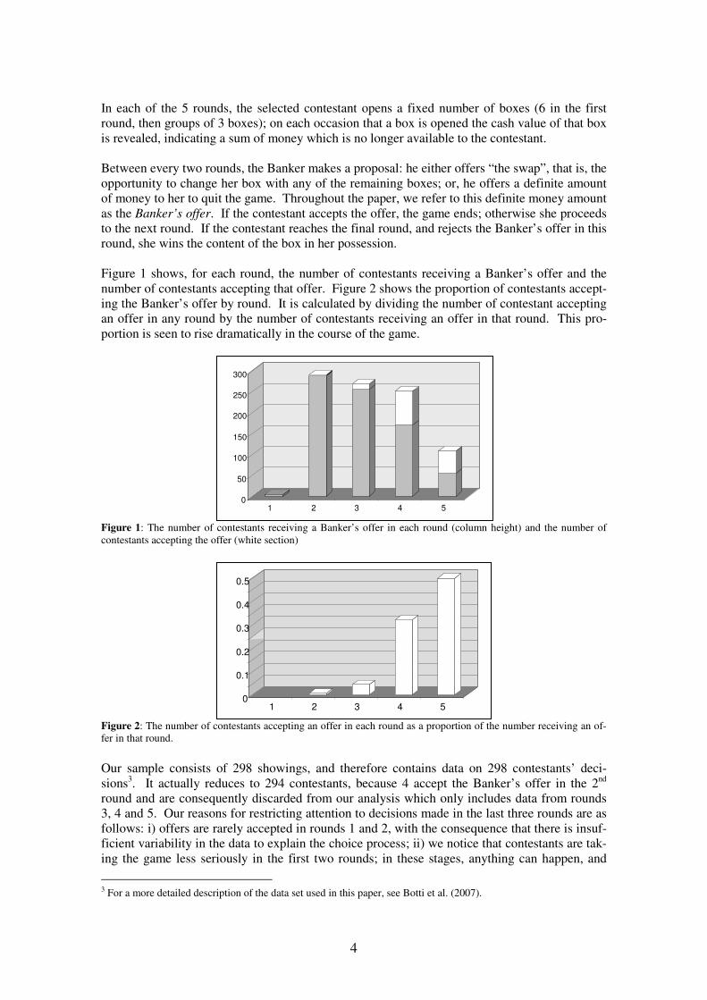
In each of the 5 rounds, the selected contestant opens a fixed number of boxes (6 in the first round, then groups of 3 boxes); on each occasion that a box is opened the cash value of that box is revealed, indicating a sum of money which is no longer available to the contestant. Between every two rounds, the Banker makes a proposal: he either offers “the swap”, that is, the opportunity to change her box with any of the remaining boxes; or, he offers a definite amount of money to her to quit the game. Throughout the paper, we refer to this definite money amount as the Banker’s offer. If the contestant accepts the offer, the game ends; otherwise she proceeds to the next round. If the contestant reaches the final round, and rejects the Banker’s offer in this round, she wins the content of the box in her possession. Figure 1 shows, for each round, the number of contestants receiving a Banker’s offer and the number of contestants accepting that offer. Figure 2 shows the proportion of contestants accept-ing the Banker’s offer by round. It is calculated by dividing the number of contestant accepting an offer in any round by the number of contestants receiving an offer in that round. This pro-portion is seen to rise dramatically in the course of the game.

Figure 1: The number of contestants receiving a Banker’s offer in each round (column height) and the number of contestants accepting the offer (white section)

Figure 2: The number of contestants accepting an offer in each round as a proportion of the number receiving an of-fer in that round.

Our sample consists of 298 showings, and therefore contains data on 298 contestants’ deci-sions3. It actually reduces to 294 contestants, because 4 accept the Banker’s offer in the 2nd round and are consequently discarded from our analysis which only includes data from rounds 3, 4 and 5. Our reasons for restricting attention to decisions made in the last three rounds are as follows: i) offers are rarely accepted in rounds 1 and 2, with the consequence that there is insuf-ficient variability in the data to explain the choice process; ii) we notice that contestants are tak-ing the game less seriously in the first two rounds; in these stages, anything can happen, and

3 For a more detailed description of the data set used in this paper, see Botti et al. (2007).

0

50

100

150

200

250

300

1 2 3 4 5

0

0.1

0.2

0.3

0.4

0.5

1 2 3 4 5

5

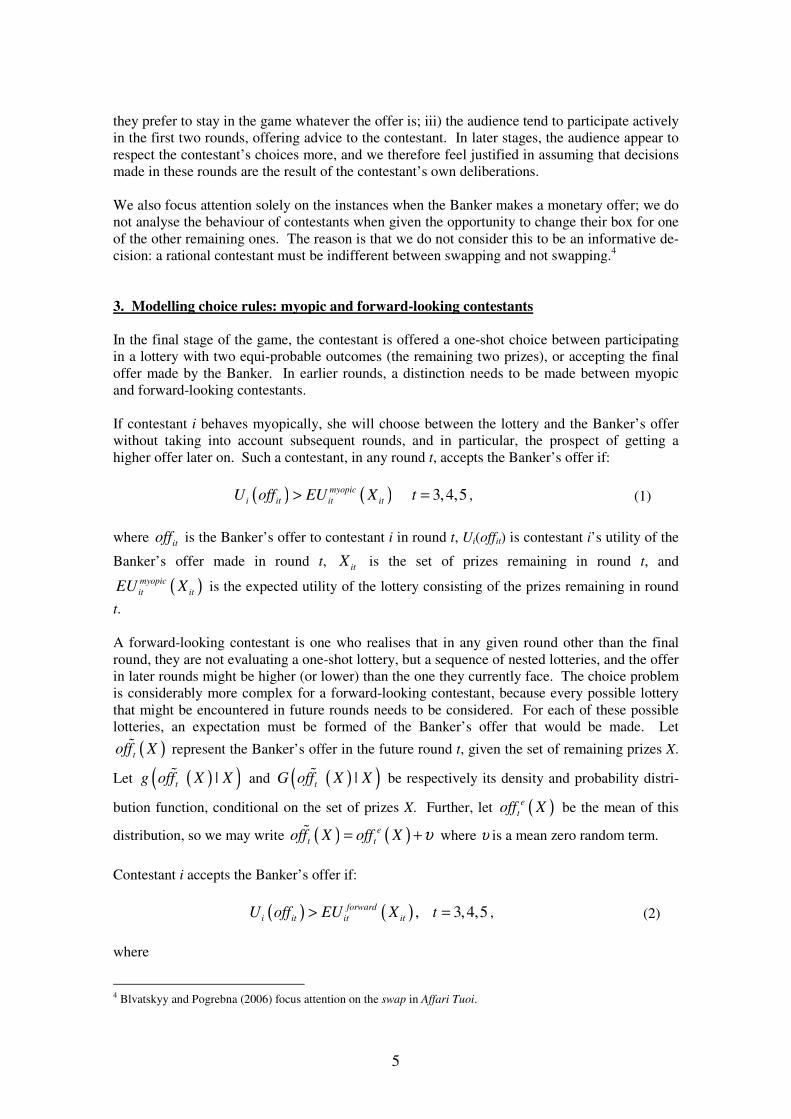
they prefer to stay in the game whatever the offer is; iii) the audience tend to participate actively in the first two rounds, offering advice to the contestant. In later stages, the audience appear to respect the contestant’s choices more, and we therefore feel justified in assuming that decisions made in these rounds are the result of the contestant’s own deliberations. We also focus attention solely on the instances when the Banker makes a monetary offer; we do not analyse the behaviour of contestants when given the opportunity to change their box for one of the other remaining ones. The reason is that we do not consider this to be an informative de-cision: a rational contestant must be indifferent between swapping and not swapping.4 3. Modelling choice rules: myopic and forward-looking contestants

In the final stage of the game, the contestant is offered a one-shot choice between participating in a lottery with two equi-probable outcomes (the remaining two prizes), or accepting the final offer made by the Banker. In earlier rounds, a distinction needs to be made between myopic and forward-looking contestants. If contestant i behaves myopically, she will choose between the lottery and the Banker’s offer without taking into account subsequent rounds, and in particular, the prospect of getting a higher offer later on. Such a contestant, in any round t, accepts the Banker’s offer if:

( ) ( ) 3,4,5myopic

i it it itU off EU X t> = , (1)

where

itoff is the Banker’s offer to contestant i in round t, Ui(offit) is contestant i’s utility of the

Banker’s offer made in round t, it

X is the set of prizes remaining in round t, and

( )myopic

it itEU X is the expected utility of the lottery consisting of the prizes remaining in round

t. A forward-looking contestant is one who realises that in any given round other than the final round, they are not evaluating a one-shot lottery, but a sequence of nested lotteries, and the offer in later rounds might be higher (or lower) than the one they currently face. The choice problem is considerably more complex for a forward-looking contestant, because every possible lottery that might be encountered in future rounds needs to be considered. For each of these possible lotteries, an expectation must be formed of the Banker’s offer that would be made. Let

( )toff Xɶ represent the Banker’s offer in the future round t, given the set of remaining prizes X.

Let ( )( )|t

g off X Xɶ and ( )( )|t

G off X Xɶ be respectively its density and probability distri-

bution function, conditional on the set of prizes X. Further, let ( )e

toff X be the mean of this

distribution, so we may write ( ) ( )e

t toff X off X υ= +ɶ where υ is a mean zero random term.

Contestant i accepts the Banker’s offer if:

( ) ( ) , 3,4,5forward

i it it itU off EU X t> = , (2)

where

4 Blvatskyy and Pogrebna (2006) focus attention on the swap in Affari Tuoi.

6

( ) ( ) ( ) ( )

( ) ( ) ( ){ }( ) ( )

56 10

3 3 4 3 5 3 31 1

10

4 4 5 4 41

5 5 5

1 1max , max ,

56 10

1max ,

10

forward

i i i j i jk i jk

j k

forward

i i i j i j

j

forward

i i i

EU X EU off X EU off X EU X

EU X EU off X EU X

EU X EU X

= =

=

=

=

=

∑ ∑

∑

ɶ ɶ

ɶ . (3)

( )forward

it itEU X is the value of continuing with the game;

( )( ) ( )( ) ( ). .t t t

EU off U off dG off

+∞

−∞

= ∫ɶ ɶ ɶ is the expected utility of the future offer; 3i jX , with

1, ,56j = … , indicates all the 56 possible lotteries deriving from the 3rd round lottery 3iX con-

testant i might face in round 4 by opening 3 of the remaining 8 boxes; 3i jkX with 1, ,10k = …

indicates all the 10 possible lotteries contestant i might face in round 5, if the lottery in round 4 were 3i j

X ; similarly 4i jX , with 1, ,10j = … , indicates all the 10 possible lotteries deriving

from the 4th round lottery 4iX contestant i might be confronted with in round 5 by opening 3 of

the remaining 5 boxes. Finally, ( )5 5forward

i iEU X is simply the probability-weighted utility of

the two outcomes remaining in round 5. A problem raised in Section 1 is that a contestant who is highly risk averse but strongly optimis-tic about future Banker’s offers may be indistinguishable from one who is highly risk loving but strongly pessimistic about future offers. We remarked there that in order to overcome this prob-lem, researchers commonly rely on the hypothesis of rational expectations. For example, de Roos and Sarafidis (2006) and Mulino et al. (2006) use data on offers made in all showings in order to form predictive equations for the Banker’s offer in each round; then, they use the pre-diction so obtained as the contestant’s belief. Post et al. (2007) do something similar. In a departure from this convention, this paper recognises that Affari tuoi provides a suitable en-vironment to estimate both preferences and beliefs in the absence of any restrictive assumptions about the way that beliefs are formed, and hence to test whether such beliefs are in fact formed according to rational expectations theory. This is possible because, in round 5, contestants’ choices do not involve any belief formation. The contestant’s problem in round 5 is just a straightforward choice between two lotteries: one with two equi-probable prizes; the other being a certainty of the Banker’s offer. It is only in rounds 3 and 4 that beliefs are formed. Under the reasonable assumption of invariance over time of contestants’ preferences, we are therefore able to combine the data from round 5 choices with that from rounds 3 and 4 in order to estimate preferences and beliefs jointly. Of course, in doing this we are making the further identifying assumption that the belief functions are the same for all contestants; in particular, that the belief functions of those who reach round 5 are the same as that of those who accept offers in previous rounds. An important point is that the distribution of the risk aversion parameter in round 5 is truncated from above, for the obvious reason that the most risk averse contestants are likely leave the game in earlier rounds. This might raise concerns of attrition or selection bias in estimation. This would indeed be a problem if we were estimating preferences using data from only round 5. But the simultaneous use of data from all three rounds enables us to estimate the complete distribution of preferences over the population. It is intuitively helpful to imagine the following sequence, which is repeated until convergence: first, the preferences of the contestants reaching round 5 are estimated; then these contestants’ choices in earlier rounds are used to deduce their

7

beliefs; the beliefs thus estimated are extended to contestants who left the game before round 5; finally, the preferences of these other contestants are deduced, filling in the truncated upper tail of the risk attitude distribution. For good measure, we have carried out extensive simulations which establish that, when estimation proceeds on this basis, the estimated distribution of pref-erences is unbiased. 4. Modelling the Banker’s offer function The hypothesis of rational expectations implies that contestants are capable of forecasting the Banker’s offer in future rounds in the same way as an econometrician with access to estimation algorithms. We therefore use data on Banker’s offers from all showings, to estimate the true of-fer function in each round. The rational expectations hypothesis can then be taken to imply that contestants form beliefs according to the estimated true offer functions. The key explanatory variable in the determination of the offer is the expected value (EV) of the remaining prizes. Here, and throughout the paper, we measure money amounts in units of €1,000. Banker’s offer in Round 4 Figure 3 shows a scatter of the round 4 offers against EV. A 450-line is super-imposed. The most obvious feature of the scatter is that the offer rises with EV. It is also noticed that the offer is nearly always far below EV. A fanning out effect is also evident, with the variance of offers rising as EV rises. In view of the strong positive skew seen in both variables, it is appropriate to take logarithms before analysing the relationship. Figure 4 shows a scatter of the logged vari-ables. Here we see that the relationship is clearly log-linear. The plot also appears homoscedas-tic. We therefore estimate the straightforward log-linear regression:

( ) ( )4 4log logoffer EV uγ β= + + , (4)

where the 4 subscripts are present since we are restricting attention to round 4. The results from estimation of (4) are:

( ) ( )

( ) ( )

ˆlog 0.460 0.857log

0.068 0.018

252

offer EV

n

= − +

=

. (5)

We may deduce from this estimated regression equation that contestants who form rational ex-pectations use the following formula for the expected offer in round 4:

( )exp 0.460 0.857logoffer EV= − + . (6)

Banker’s Offer in Round 5 Figure 5 shows offer against expected value for all offers made in round 5. A 450-line is again super-imposed. Again it is also clear that the offer rarely exceeds the expected value. However, a difference from round 4 is that some points appear to be on (or very close to) the 450-line, im-plying that the offer exactly equals the expected value. We shall treat these observations as up-per-censored observations. Note that this censoring tends to arise when the expected value is

8

comparatively low. When the expected value is high, the offer is usually below the expected value.

Figure 3: Offer against expected value in round 4. 45°-line superimposed.

-4-2

02

4lo

goffe

r

-4 -2 0 2 4 6logev

Figure 4: Logarithm of offer against logarithm of expected value in round 4. 45°-line superimposed.

Figure 5: Offer against expected value in round 5. 45°-line superimposed.

9

-10

-50

5lo

g o

ffer

-10 -5 0 5log of expected value

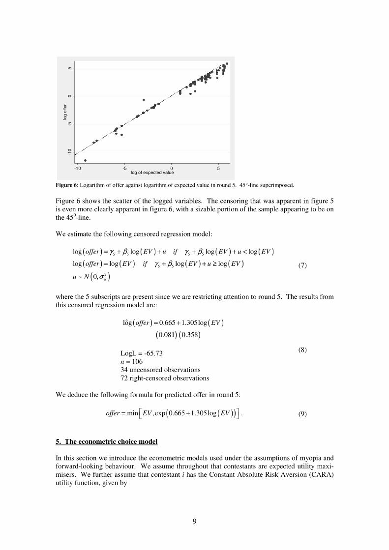
Figure 6: Logarithm of offer against logarithm of expected value in round 5. 45°-line superimposed. Figure 6 shows the scatter of the logged variables. The censoring that was apparent in figure 5 is even more clearly apparent in figure 6, with a sizable portion of the sample appearing to be on the 450-line. We estimate the following censored regression model:

( ) ( ) ( ) ( )

( ) ( ) ( ) ( )

( )

5 5 5 5

5 5

2

log log log log

log log log log

~ 0, u

offer EV u if EV u EV

offer EV if EV u EV

u N

γ β γ β

γ β

σ

= + + + + <

= + + ≥ (7)

where the 5 subscripts are present since we are restricting attention to round 5. The results from this censored regression model are:

( ) ( )

( ) ( )

ˆlog 0.665 1.305log

0.081 0.358

offer EV= +

LogL = -65.73 n = 106 34 uncensored observations 72 right-censored observations

(8)

We deduce the following formula for predicted offer in round 5:

( )( )min ,exp 0.665 1.305logoffer EV EV = + . (9)

5. The econometric choice model

In this section we introduce the econometric models used under the assumptions of myopia and forward-looking behaviour. We assume throughout that contestants are expected utility maxi-misers. We further assume that contestant i has the Constant Absolute Risk Aversion (CARA) utility function, given by

10

exp( )( ) i

i

i

r xU x

r

− −= , (10)

where x is the outcome and ri is the coefficient of absolute risk aversion for contestant i. We as-sume, in the spirit of Holt and Laury (2002), that this coefficient is distributed across the popu-

lation according to ( )2~ ,i r r

r N µ σ . Since the utility function is unique up to a monotonic trans-

formation, identification requires that we normalise the utility function to:

( )( )( )

1 exp( )

1 exp maxi

i

i

r xU x

r x

− −=

− −, (11)

so that ( )0 0iU = and ( )( )max 1iU x = , where max(x) is the highest prize in the game, namely,

€500,000. According to the condition specified in (1), contestant i accepts the Banker’s offer when-ever 0

ity

∗ > , whereit

y∗ , in the myopic model, is defined by

( ) ( )myopic

it i it it it ity U off EU X ε∗ = − + . (12)

Here it

ε is a Fechner-type error term (Hey and Orme, 1994), with ( )2~ 0,it

N εε σ . It has the

interpretation of a computational error in calculating utilities and expected utilities. This error is assumed to be homoscedastic and uncorrelated with all other variables in the model. Turning to forward-looking behaviour, let us first assume that the future offer function has a de-generate distribution, so that the error term υ introduced in Section 3 is identically zero, and contestants place a probability of 1 on the event that the future offer equals the expected value

of the offer, e

t toff off=ɶ .5 It follows that the expected utility of the future offer in (3) collapses

simply to the utility of the expected offer:

( )( ) ( )( ). .e

t tEU off U off=ɶ . (13)

Given this assumption, the latent variable underlying the choice for a forward-looking contest-ant is

( ) ( )forward

it i t it it ity U off EU X ε∗ = − + . (14)

Let us define the binary variable yit to take the value 1 if contestant i accepts the Banker’s offer in round t, and the value -1 otherwise. The relationship between the observable variable yit and the latent variable

ity

∗ is then given by:

1it

y = if 0>∗ity

1it

y = − if 0≤∗ity .

(15)

5 This assumption is relaxed in Section 9 below, where we assume that the stochastic term υ has a positive variance.

11

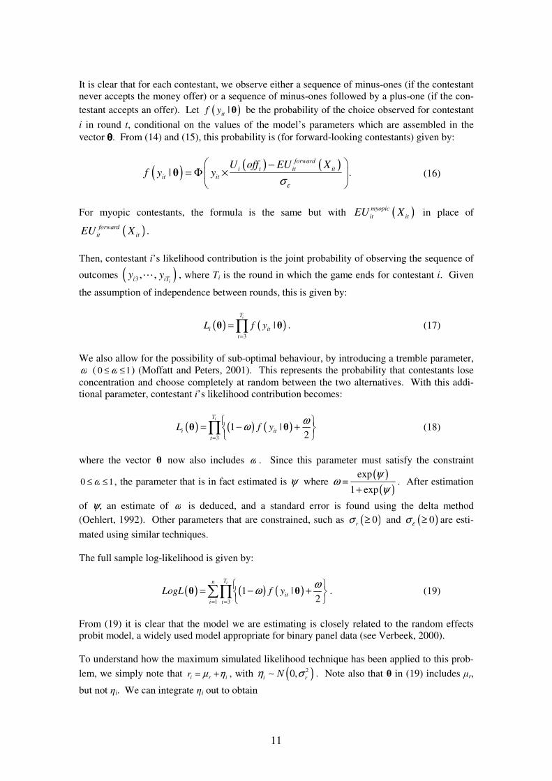
It is clear that for each contestant, we observe either a sequence of minus-ones (if the contestant never accepts the money offer) or a sequence of minus-ones followed by a plus-one (if the con-testant accepts an offer). Let ( )|itf y θ be the probability of the choice observed for contestant

i in round t, conditional on the values of the model’s parameters which are assembled in the vector θθθθ. From (14) and (15), this probability is (for forward-looking contestants) given by:

( )( ) ( )

|forward

i t it it

it it

U off EU Xf y y

εσ

−= Φ ×

θ . (16)

For myopic contestants, the formula is the same but with ( )myopic

it itEU X in place of

( )forward

it itEU X .

Then, contestant i’s likelihood contribution is the joint probability of observing the sequence of

outcomes ( )3 , ,ii iT

y y⋯ , where Ti is the round in which the game ends for contestant i. Given

the assumption of independence between rounds, this is given by:

( ) ( )3

|iT

i it

t

L f y=

= ∏θ θ . (17)

We also allow for the possibility of sub-optimal behaviour, by introducing a tremble parameter, ω ( 10 ≤≤ ω ) (Moffatt and Peters, 2001). This represents the probability that contestants lose concentration and choose completely at random between the two alternatives. With this addi-tional parameter, contestant i’s likelihood contribution becomes:

( ) ( ) ( )3

1 |2

iT

i it

t

L f yω

ω=

= − +

∏θ θ (18)

where the vector θ now also includes ω . Since this parameter must satisfy the constraint

10 ≤≤ ω , the parameter that is in fact estimated is ψ where ( )

( )exp

1 exp

ψω

ψ=

+. After estimation

of ψ, an estimate of ω is deduced, and a standard error is found using the delta method (Oehlert, 1992). Other parameters that are constrained, such as ( )0rσ ≥ and ( )0εσ ≥ are esti-

mated using similar techniques. The full sample log-likelihood is given by:

( ) ( ) ( )1 3

1 |2

iTn

it

i t

LogL f yω

ω= =

= − +

∑∏θ θ . (19)

From (19) it is clear that the model we are estimating is closely related to the random effects probit model, a widely used model appropriate for binary panel data (see Verbeek, 2000). To understand how the maximum simulated likelihood technique has been applied to this prob-

lem, we simply note that irir ηµ += , with ( )20,i r

Nη σ∼ . Note also that θ in (19) includes µr,

but not ηi. We can integrate ηi out to obtain

12

( ) ( ) ( )3

11 ,

2

iT

ii it i i

t r r

L f y dηω

ω η φ ησ σ

+∞

=−∞

= − +

∏∫θ θ . (20)

Following Lerman and Manski (1981), this integral can be approximated by a sample average of the integrand computed drawing R numbers from a standard normal distribution. This way we obtain an unbiased estimator of the integral in (20), with a variance that goes to zero as R in-creases. 6. Estimation of the choice models and a test of rational expectations

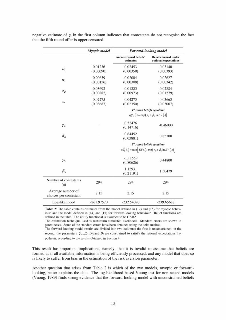
In this Section, we separately estimate the two models constructed in the previous section, using the method of maximum simulated likelihood. Our sample consists of 294 players observed making 2.15 choices on average. In each model, integration over ir is performed by simulation using 100 draws for each contestant based on Halton sequences (Train, 2003). We adopt this procedure in preference to the more commonly used Gauss-Hermite quadrature, since, given the complexity of the model, the computational burden is considerably lower for the former than for the latter. Table 2 presents the estimates for both of the models, myopic and forward-looking, with a CARA specification.6 Results from the myopic model are presented in the first column. Re-sults from the forward-looking model are divided into two columns. The first of these contains the results of the model estimated with all parameters unconstrained. The second column shows the results obtained with the parameters of the belief functions constrained according to (6) and (9), that is, when contestants are assumed to form rational expectations of the offers in rounds 4 and 5. As expected, the mean of the risk attitude parameter, rµ , differs significantly between the two models, being of approximately twice the magnitude in the forward-looking model. The sig-nificantly positive estimates of rσ vindicate the assumption of varying risk attitude over the population. The Fechner error parameter, εσ , is also significantly different from zero in two of the three models. However, in the (unconstrained) forward-looking model, it takes a much smaller value and is not significant. This suggests that, after allowing for heterogeneity in the risk aversion parameter, very little measurement error remains to be explained. Finally, the tremble parameter is statistically significant. Its magnitude (in the unconstrained forward-looking model) indicates that contestants lose concentration on around 4% of occasions. This is in line with estimates obtained elsewhere in the literature (see, for example, Loomes et al., 2002). Constraining the parameters of the belief function as done in the final column of Table 2 is in line with the approach of other researchers already cited in Sections 1 and 3. Here, we note that on the evidence of a likelihood ratio test comparing the two columns (χ2(4) = 14.24; p = 0.008), there is a significant difference between the parameters actually used by contestants to form be-liefs (column 2) and those estimated using all the available information (column 3). This test result amounts to a strong rejection of the rational expectations hypothesis. In particular, the

6 We have also estimated the two models with a CRRA and an Expo-power specification, assuming a non-zero life-time wealth as a parameter to be estimated in the models, along similar lines to Andersen et al. (2006). We find that the estimate of the lifetime wealth parameter is significantly different from zero only in the myopic CRRA specifica-tion, in this case taking a value close to €20,000. However, the use of these specifications never significantly im-proves the fit over the CARA specification (cf Andersen et al, 2006; de Roos and Sarafidis, 2006; Post et al, 2007). The various results are available from the authors upon request.

13

negative estimate of γ5 in the first column indicates that contestants do not recognise the fact that the fifth round offer is upper censored.

Myopic model Forward-looking model

unconstrained beliefs’

estimates

Beliefs formed under

rational expectations

rµ 0.01236

(0.00090) 0.02453

(0.00358) 0.03140

(0.00393)

rσ 0.00639

(0.00156) 0.02004

(0.00308) 0.02627

(0.00342)

εσ 0.03692 (0.00882)

0.01225 (0.00973)

0.02884 (0.01279)

ω 0.07275 (0.03687)

0.04275 (0.02350)

0.03663 (0.03007)

4th round beliefs equation:

( ) ( )( )4 4 4. exp ln .off EVγ β= +ɶ

4γ - 0.52476 (0.14716)

-0.46000

4β - 0.64452 (0.03881) 0.85700

5th round beliefs equation:

( ) ( ) ( )( )5 5 5. min . ,exp ln .off EV EVγ β = +

ɶ

5γ - -1.11559 (0.80626) 0.44800

5β - 1.12931 (0.21191) 1.30479

Number of contestants (n)

294 294 294

Average number of choices per contestant

2.15 2.15 2.15

Log-likelihood -261.97520 -232.54020 -239.65688

Table 2: The table contains estimates from the model defined in (12) and (15) for myopic behav-iour, and the model defined in (14) and (15) for forward-looking behaviour. Belief functions are defined in the table. The utility functional is assumed to be CARA. The estimation technique used is maximum simulated likelihood. Standard errors are shown in parentheses. Some of the standard errors have been obtained using the delta method. The forward-looking model results are divided into two columns: the first is unconstrained; in the second, the parameters 4γ ,β4 , 5γ and β5 are constrained to satisfy the rational expectations hy-

pothesis, according to the results obtained in Section 4.

This result has important implications, namely, that it is invalid to assume that beliefs are formed as if all available information is being efficiently processed, and any model that does so is likely to suffer from bias in the estimation of the risk aversion parameter. Another question that arises from Table 2 is which of the two models, myopic or forward-looking, better explains the data. The log-likelihood based Vuong test for non-nested models (Vuong, 1989) finds strong evidence that the forward-looking model with unconstrained beliefs

14

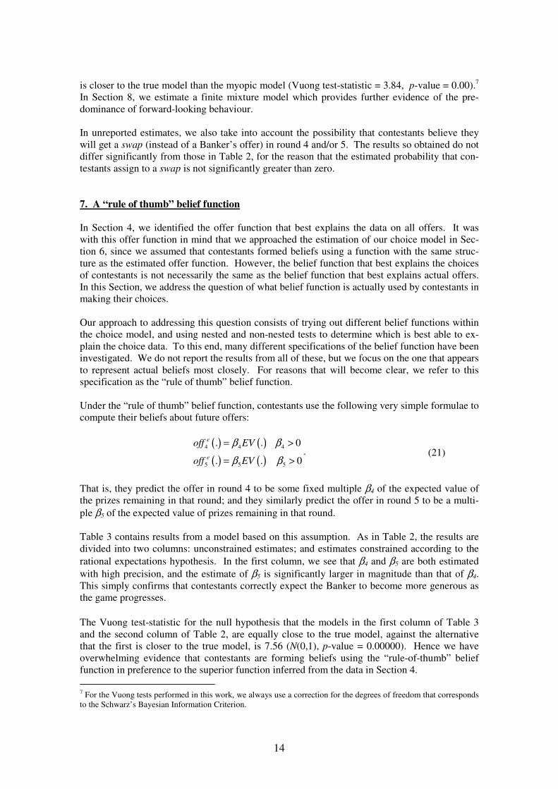
is closer to the true model than the myopic model (Vuong test-statistic = 3.84, p-value = 0.00).7 In Section 8, we estimate a finite mixture model which provides further evidence of the pre-dominance of forward-looking behaviour. In unreported estimates, we also take into account the possibility that contestants believe they will get a swap (instead of a Banker’s offer) in round 4 and/or 5. The results so obtained do not differ significantly from those in Table 2, for the reason that the estimated probability that con-testants assign to a swap is not significantly greater than zero. 7. A “rule of thumb” belief function In Section 4, we identified the offer function that best explains the data on all offers. It was with this offer function in mind that we approached the estimation of our choice model in Sec-tion 6, since we assumed that contestants formed beliefs using a function with the same struc-ture as the estimated offer function. However, the belief function that best explains the choices of contestants is not necessarily the same as the belief function that best explains actual offers. In this Section, we address the question of what belief function is actually used by contestants in making their choices. Our approach to addressing this question consists of trying out different belief functions within the choice model, and using nested and non-nested tests to determine which is best able to ex-plain the choice data. To this end, many different specifications of the belief function have been investigated. We do not report the results from all of these, but we focus on the one that appears to represent actual beliefs most closely. For reasons that will become clear, we refer to this specification as the “rule of thumb” belief function. Under the “rule of thumb” belief function, contestants use the following very simple formulae to compute their beliefs about future offers:

( ) ( )

( ) ( )4 4 4

5 5 5

. . 0

. . 0

e

e

off EV

off EV

β β

β β

= >

= >. (21)

That is, they predict the offer in round 4 to be some fixed multiple β4 of the expected value of the prizes remaining in that round; and they similarly predict the offer in round 5 to be a multi-ple β5 of the expected value of prizes remaining in that round. Table 3 contains results from a model based on this assumption. As in Table 2, the results are divided into two columns: unconstrained estimates; and estimates constrained according to the rational expectations hypothesis. In the first column, we see that β4 and β5 are both estimated with high precision, and the estimate of β5 is significantly larger in magnitude than that of β4. This simply confirms that contestants correctly expect the Banker to become more generous as the game progresses. The Vuong test-statistic for the null hypothesis that the models in the first column of Table 3 and the second column of Table 2, are equally close to the true model, against the alternative that the first is closer to the true model, is 7.56 (N(0,1), p-value = 0.00000). Hence we have overwhelming evidence that contestants are forming beliefs using the “rule-of-thumb” belief function in preference to the superior function inferred from the data in Section 4. 7 For the Vuong tests performed in this work, we always use a correction for the degrees of freedom that corresponds to the Schwarz’s Bayesian Information Criterion.

15

Forward-looking model with “rule of thumb” beliefs

unconstrained beliefs’ esti-

mates

Beliefs formed under ra-

tional expectations

rµ 0.02410

(0.00216) 0.02335

(0.00172)

rσ 0.01778

(0.00196) 0.01633

(0.00142)

εσ 0.01284 (0.01099)

0.01956 (0.00788)

ω 0.06185 (0.02701)

0.05910 (0.02516)

4th round beliefs equation: ( ) ( )4 4. .off EVβ=ɶ

4β 0.38340 (0.02901)

0.33170

5th round beliefs equation: ( ) ( )5 5. .off EVβ=ɶ

5β 0.54627 (0.04672)

0.56674

Number of contest-ants (n)

294 294

Average number of choices per contest-

ant 2.15 2.15

Log-likelihood -235.54346 -236.52784

Table 3: Estimates from the model defined in (14), (15) and (21). The utility func-tional is assumed to be CARA. The estimation technique used is maximum simulated likelihood. Standard errors are shown in parentheses. Some of the standard errors have been obtained using the delta method. The forward-looking model results are divided into two columns: the first is uncon-strained; in the second, the parameters β4 and β5 are constrained to satisfy the ra-tional expectations hypothesis.

The second column of the table shows the estimates of the model with the parameters β4 and β5 constrained to equal the values obtained by performing (external) regressions of actual offer on EV, using the entire data set. We firstly see that the estimates obtained in the unconstrained model are not significantly different from those obtained in the external regressions, which is loosely consistent with the rational expectations hypothesis. We further note that a likelihood ratio test of the hypothesis that the parameters exactly equal their external estimates gives the

( )2 2χ statistic ( )2 236.53 235.54 1.97× − = , which is not significant at any reasonable level.

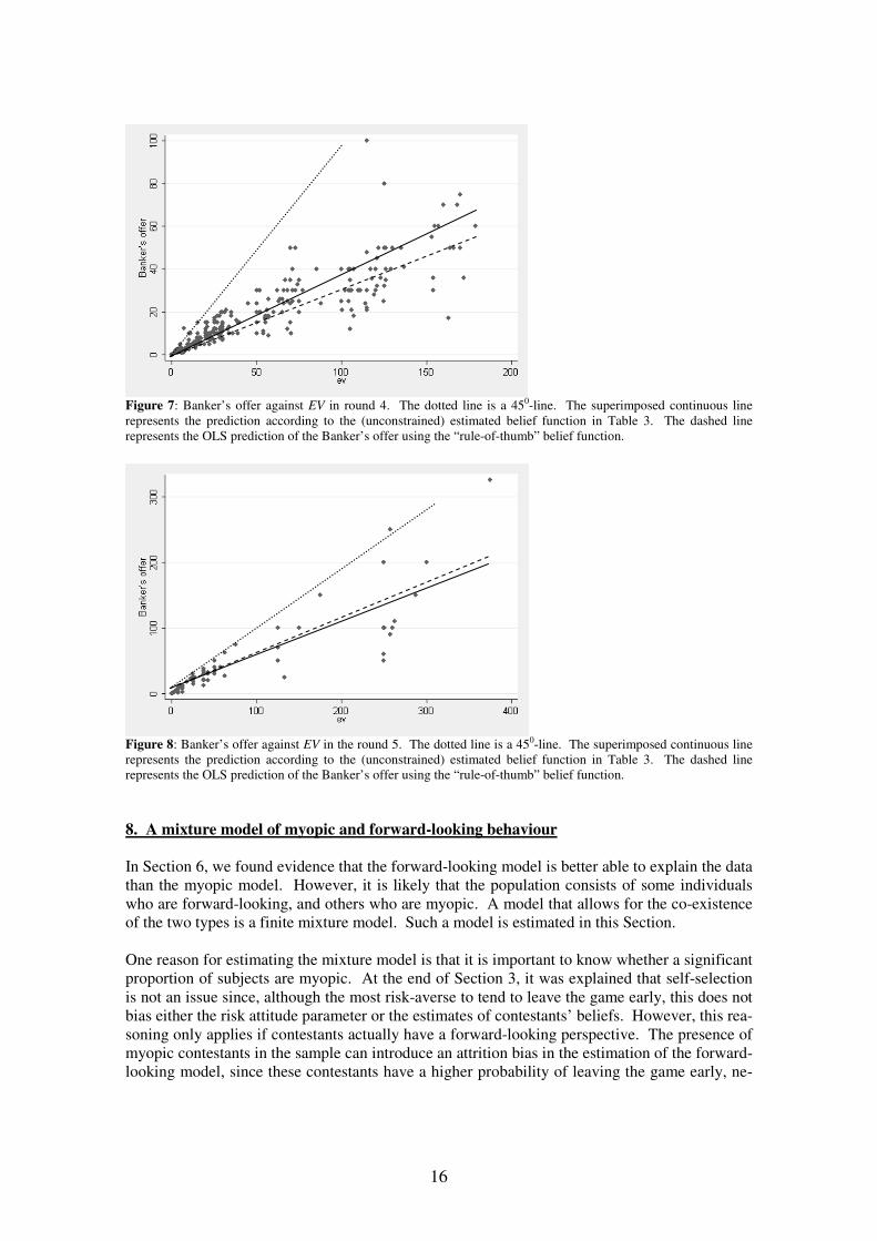
We therefore conclude that we have no evidence to reject the hypothesis of rational expecta-tions, under the auxiliary hypothesis of the “rule-of-thumb” belief function. Figures 7 and 8 present, for rounds 4 and 5 respectively, graphical comparisons between the “rule-of-thumb” belief functions estimated using the model, and those estimated externally us-ing actual offers, data on which is also shown in the graphs. In each case, we see that the esti-mated belief function is impressively close to the external estimate, providing further evidence in favour of rational expectations with “rule-of-thumb” beliefs.

16

Figure 7: Banker’s offer against EV in round 4. The dotted line is a 450-line. The superimposed continuous line represents the prediction according to the (unconstrained) estimated belief function in Table 3. The dashed line represents the OLS prediction of the Banker’s offer using the “rule-of-thumb” belief function.

Figure 8: Banker’s offer against EV in the round 5. The dotted line is a 450-line. The superimposed continuous line represents the prediction according to the (unconstrained) estimated belief function in Table 3. The dashed line represents the OLS prediction of the Banker’s offer using the “rule-of-thumb” belief function. 8. A mixture model of myopic and forward-looking behaviour

In Section 6, we found evidence that the forward-looking model is better able to explain the data than the myopic model. However, it is likely that the population consists of some individuals who are forward-looking, and others who are myopic. A model that allows for the co-existence of the two types is a finite mixture model. Such a model is estimated in this Section. One reason for estimating the mixture model is that it is important to know whether a significant proportion of subjects are myopic. At the end of Section 3, it was explained that self-selection is not an issue since, although the most risk-averse to tend to leave the game early, this does not bias either the risk attitude parameter or the estimates of contestants’ beliefs. However, this rea-soning only applies if contestants actually have a forward-looking perspective. The presence of myopic contestants in the sample can introduce an attrition bias in the estimation of the forward-looking model, since these contestants have a higher probability of leaving the game early, ne-

17

glecting the prospect of generous offers in later rounds. Ideally, therefore, we hope for the pro-portion of myopic subjects to be zero.

Let myopiciL be contestant i’s likelihood contribution in (20) under the hypothesis that she be-

haves myopically, and let forwardiL be likewise under the assumption of forward-looking behav-

iour. In addition, let ( )0 1π π≤ ≤ be the mixing proportion, which is the proportion of the

population who are forward-looking. Contestant i’s likelihood contribution in the mixture model is then:

( ) forwardi

myopici

mixturei LLL ππ +−= 1 . (22)

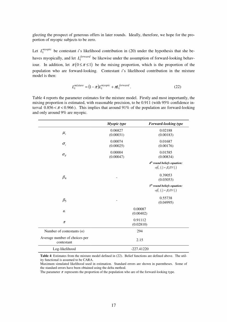
Table 4 reports the parameter estimates for the mixture model. Firstly and most importantly, the mixing proportion is estimated, with reasonable precision, to be 0.911 (with 95% confidence in-terval 0.856 0.966π< < ). This implies that around 91% of the population are forward-looking and only around 9% are myopic.

Myopic type Forward-looking type

rµ 0.06827

(0.00031) 0.02188

(0.00183)

rσ 0.00074

(0.00025) 0.01687

(0.00176)

εσ 0.00004 (0.00047)

0.01585 (0.00834)

4th round beliefs equation:

( ) ( )4 4. .off EVβ=ɶ

4β - 0.39053

(0.03053)

5th round beliefs equation:

( ) ( )5 5. .off EVβ=ɶ

5β - 0.55738

(0.04995)

ω 0.00087 (0.00402)

π 0.91112 (0.02810)

Number of contestants (n) 294

Average number of choices per contestant

2.15

Log-likelihood -227.41220

Table 4: Estimates from the mixture model defined in (22). Belief functions are defined above. The util-ity functional is assumed to be CARA. Maximum simulated likelihood used in estimation. Standard errors are shown in parentheses. Some of the standard errors have been obtained using the delta method. The parameter π represents the proportion of the population who are of the forward-looking type.

18

Comparing the estimates of mean risk attitude (r

µ ) for the two types, we note first that myopic types are more risk averse than forward-looking types. We further note that the estimate of

rµ for myopic individuals (0.068) is almost six times as large as that estimated on the assump-tion that all subjects are myopic (0.012; Table 2 above). The explanation for this difference is straightforward: when the myopic model is forced to explain the behaviour of forward-looking individuals, their tendency to reject Banker’s offers is interpreted as straightforward risk-lovingness, and it is inevitable that the estimate of the risk aversion parameter will be very low.8 The estimated standard deviation of risk attitude, rσ , for myopic types, is smaller in the mixture model (0.00074), than in the model assuming all individuals are myopic (0.006; Table 2, first column). This difference simply reflects the fact that the two types differ quite markedly in their risk attitude, so a model that assumes all individuals are of one type will inevitably over-estimate the spread of risk attitude. The estimates obtained in the mixture model of

rµ and rσ

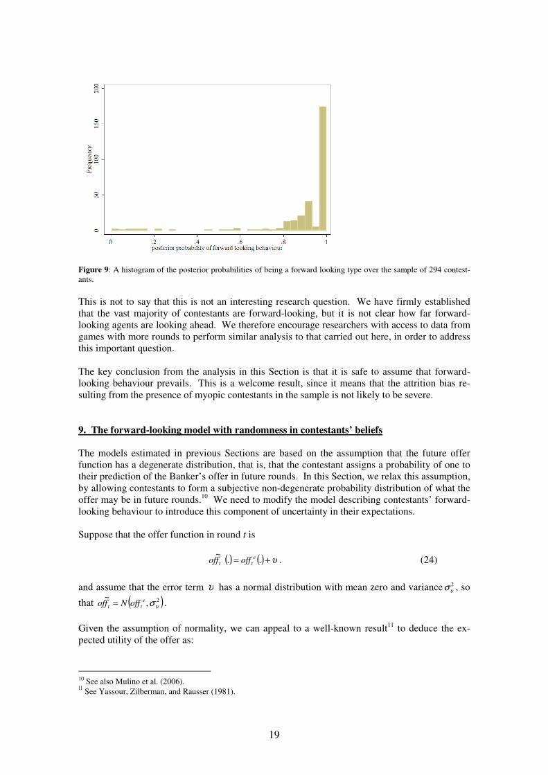
for forward-looking types are very close to the estimates obtained in the model that assumes that all individuals are forward-looking with “rule-of-thumb” beliefs (Table 3, second column). This is for the simple reason that the majority of individuals are forward-looking, as indicated by our high estimate of π in the mixture model. The same reasoning applies to the two parame-ters 4β and 5β , whose estimates under the mixture model agree closely with those in Table 3. The magnitude of the computational error, as represented by εσ , is still small in the mixture model, but is significantly smaller for myopic types (0.00004), than in the model that assumes all individuals are myopic (0.037; Table 2, first column). The reason for this is similar to that advanced above in the context of the parameter rσ . The tremble probability, ω , is assumed to be the same for both types in the mixture model9, and we see that its estimate is very small and insignificant. The posterior probability of each contestant being of the forward-looking type is computed us-ing Bayes’ rule, as follows:

( )3 , ,i

forward

i

i iT mixture

i

LP i forward y y

L

π= =⋯ , (23)

Its distribution over the 294 contestants is shown in Figure 9. As expected, the majority of con-testants have a high posterior probability of being of the forward-looking type. In unreported work, we also estimate the choice model under the hypothesis that contestants are not fully forward-looking, but look just one-step-ahead. That is, when in round 3 they only con-sider all the possible lotteries and the consequent offers they might get in round 4. Unfortu-nately, Affari Tuoi is such that the sequence of rounds is not sufficiently long to capture the dif-ference between the one-step-ahead model and the forward-looking one; these two models pre-dict different behaviour only in round 3. A mixture model has been estimated with these two types, and another model estimated with the myopic model as a third type. These mixture mod-els fail to converge, and we attribute this to the inability of the data to distinguish between the two types of forward-looking behaviour.

8 See de Roos and Sarafidis (2006) and Mulino et al. (2006) for a more detailed explanation. 9 We know of no reason to presume that one type of individual trembles more than the other.

19

Figure 9: A histogram of the posterior probabilities of being a forward looking type over the sample of 294 contest-ants. This is not to say that this is not an interesting research question. We have firmly established that the vast majority of contestants are forward-looking, but it is not clear how far forward-looking agents are looking ahead. We therefore encourage researchers with access to data from games with more rounds to perform similar analysis to that carried out here, in order to address this important question. The key conclusion from the analysis in this Section is that it is safe to assume that forward-looking behaviour prevails. This is a welcome result, since it means that the attrition bias re-sulting from the presence of myopic contestants in the sample is not likely to be severe. 9. The forward-looking model with randomness in contestants’ beliefs The models estimated in previous Sections are based on the assumption that the future offer function has a degenerate distribution, that is, that the contestant assigns a probability of one to their prediction of the Banker’s offer in future rounds. In this Section, we relax this assumption, by allowing contestants to form a subjective non-degenerate probability distribution of what the offer may be in future rounds.10 We need to modify the model describing contestants’ forward-looking behaviour to introduce this component of uncertainty in their expectations. Suppose that the offer function in round t is

( ) ( ) υ+= ..~ e

tt offfof . (24) and assume that the error term υ has a normal distribution with mean zero and variance 2

υσ , so

that ( )2,~

υσe

tt offNfof = . Given the assumption of normality, we can appeal to a well-known result11 to deduce the ex-pected utility of the offer as:

10 See also Mulino et al. (2006). 11 See Yassour, Zilberman, and Rausser (1981).

20

( )( )( ) 2 2exp .

. exp2

e

i t ii t

i

roff rEU off

r

υσ − = −

ɶ . (25)

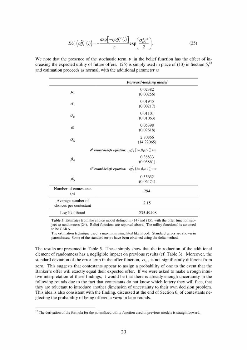
We note that the presence of the stochastic term υ in the belief function has the effect of in-creasing the expected utility of future offers. (25) is simply used in place of (13) in Section 5,12 and estimation proceeds as normal, with the additional parameter υ.

Forward-looking model

rµ 0.02382

(0.00256)

rσ 0.01945

(0.00217)

εσ 0.01101 (0.01063)

ω 0.05398 (0.02618)

υσ 2.70866 (14.22065)

4th round beliefs equation: ( ) ( ) υβ += ..~

44 EVfof

4β 0.38833 (0.03861)

5th round beliefs equation: ( ) ( ) υβ += ..~

55 EVfof

5β 0.55632 (0.06474)

Number of contestants (n)

294

Average number of choices per contestant

2.15

Log-likelihood -235.49498

Table 5: Estimates from the choice model defined in (14) and (15), with the offer function sub-ject to randomness (24). Belief functions are reported above. The utility functional is assumed to be CARA. The estimation technique used is maximum simulated likelihood. Standard errors are shown in parentheses. Some of the standard errors have been obtained using the delta method.

The results are presented in Table 5. These simply show that the introduction of the additional element of randomness has a negligible impact on previous results (cf. Table 3). Moreover, the standard deviation of the error term in the offer function, υσ , is not significantly different from zero. This suggests that contestants appear to assign a probability of one to the event that the Banker’s offer will exactly equal their expected offer. If we were asked to make a rough intui-tive interpretation of these findings, it would be that there is already enough uncertainty in the following rounds due to the fact that contestants do not know which lottery they will face, that they are reluctant to introduce another dimension of uncertainty to their own decision problem. This idea is also consistent with the finding, discussed at the end of Section 6, of contestants ne-glecting the probability of being offered a swap in later rounds.

12 The derivation of the formula for the normalized utility function used in previous models is straightforward.

21

10. Conclusion Research using game-show data has not been without criticism. Leaving aside the criticism of non-representativeness of the sample, a concern frequently raised is that contestants are behav-ing strategically, inferring information on the content of their box from the Banker’s behaviour (since it is a known fact that the Banker knows the content of each individual box). In anticipa-tion of this criticism, we have used the offer data to test the hypothesis that the Banker’s offer depends positively on the amount that is in the current contestant’s box, controlling for the av-erage of the remaining prizes. We find this effect to be positive but very small in magnitude, leading us to conclude that little information can be inferred from the Banker’s offer. Bom-bardini and Trebbi (2007) obtain a similar result using data from the same game. This evidence leads us to conclude that strategic behaviour is not an important issue. One important conclusion of this paper, established forcefully through the mixture model esti-mated in Section 8, is that the vast majority of subjects are forward-looking, meaning that they take into account expectations of the Banker’s offer in future rounds when making their choice in the current round. This finding confirms the importance of the role of contestants’ beliefs, and of discovering how these beliefs are formed. The econometric problem of estimating the belief function has been the principal focus of the paper. One result (established in Section 9) is that beliefs are deterministic: once a belief has been formed about the Banker’s offer in a particular round, the contestant assigns a probability of one to this value. More importantly, we have been interested in whether such beliefs are formed in accordance with the rational expectations hypothesis. In order to test the rational ex-pectations hypothesis, we have compared the belief function estimated within the choice model to the “true” offer function estimated using the complete data set of Banker’s offers. A problem with this approach that was not raised earlier is that, in order to implement the assumption of rational expectations, we are implicitly assuming that each contestant has access to the complete set of Banker’s offers. The obvious logical problem with this assumption is that contestants cannot possibly know what offers are made in future games; they can only know about offers that have been made previously to their own participation. However, we are following other re-searchers (e.g. Deck et al., 2006; Mulino et al., 2006; Post et al., 2007) in assuming that all in-formation, including future offers, is available. In any case, the principal objective of this paper has not been to estimate the rational expecta-tions model, but rather to test the rational expectations hypothesis using a more general model. Our unconstrained model is fully flexible in terms of the parameter values in the belief function, which is estimated within the choice model, and therefore should tell us how beliefs are actually formed, on the basis of information which is actually available to the contestant at the time deci-sions are made. One of our principal findings has been that, at least in the context of Affari

Tuoi, the estimates of the belief function in the unconstrained model do not closely match the estimates of the offer function obtained using sophisticated processing of the offer data. There-fore, constraining the choice model to incorporate the estimated offer function results in biased estimation of the preference parameters. However, the situation in which we found the belief function to differ from the true offer func-tion was under the assumption of an optimal structure of the offer function, including all of the features, for example upper-censoring, that are apparent in the offer data. When a less elaborate structure is assumed for the belief function, in which it is simply assumed that contestants be-lieve that the offer at a given stage of the game will be a fixed multiple of the expected prize, we find that the belief function estimated within the choice model is not significantly different from that estimated from data on actual offers. We have referred to such beliefs as being determined by the “rule-of-thumb” belief function.

22

Hence we are led to the conclusion that, again in the context of Affari Tuoi, contestants are ra-tional up to a point. They appear to be using all of the information that is available (i.e. all of the offer data), but they do not appear to be using it in an optimal way. Of course, a different conclusion may be reached in the analysis of data from other game shows. Our recommendation to other researchers is that it is always desirable to estimate the belief function in an unconstrained way as a component of the choice model, rather than to rely on prior assumptions about the manner in which such beliefs are formed.

23

References

Andersen, S., Harrison, G. W., Lau M. I. and E. E. Rutström (2006) “Dynamic choice behavior in a natural experiment”, University of Central Florida, Economics Department, work-

ing paper 06-10, 1-54. Andersen, S., Harrison, G. W., Lau M. I. and E. E. Rutström (2007) “Risk aversion in game

shows”, forthcoming, J. C. Cox and G. W. Harrison (eds.), Risk Aversion in Experi-

ments (Greenwich, CT: JAI Press, Research in Experimental Economics, Volume 12) Attfield C.L.F., D. Demery and N.W.Duck, 1991, Rational Expectations in Macroeconomics,

Second Edition, Blackwell, Oxford, UK. Baltagi, B.H. (2001), Econometric analysis of panel data, Second Edition, Wiley: Chichester,

UK. Beetma, R. and Shotman P. (2001), “Measuring risk attitudes in a natural experiment: data from

the television game show Lingo”, Economic Journal, 111, 821-848. Bellemare, C., Kröger, S. and A. van Soest (2005), “Actions and Beliefs: estimating distribu-

tion-based preferences using large scale experiment with probability questions on ex-pectations”, CIRPÉE, Cahier de recherche/Working Paper 05-23

Blvatskyy, P., Pogrebna G. (2006) “Loss aversion? Not with half-a-million on the table!”, Insti-tute of Empirical Research in Economics, Working Paper Series, n. 274, University of Zurich,

Bombardini, M., Trebbi, F. (2007), “Risk aversion and EU theory: a field experiment with large and small stakes”, Mimeo.

Botti, F., Conte, A., Di Cagno, D. and D’Ippoliti, C. (2007), “Risk aversion, demographics and unobserved heterogeneity. Evidence from the Italian TV Show “Affari Tuoi””, forth-coming in Innocenti A. e Sbriglia P. (eds.), Games, Rationality and Behaviour, Hound-mills: Palgrave MacMillan.

Conte A., Hey J. D. and Moffatt P. G. (2007), “Mixture models of choice under risk”, Univer-sity of York, Discussion Papers in Economics, N. 2007/06.

Deck, C., Jungmin, L. and J. Reyes, (2006), “Risk attitude in large stake gambles: Evidence from a game show”, Working Paper, Department of Economics, University of Arkan-sas.

de Roos, N. and S. Sarafidis (2006), “Decision making under risk in Deal or No Deal”, Working

Paper, School of Economics and Political Science, University of Sydney. Friend, I., and Blume M. B. (1975), “The demand for risky assets”, American Economic Re-

view, 65, 900-922. Gertner, R. (1993) “Game shows and economic behaviour: risk taking on “Card sharks””, The

Quarterly Journal of Economics, 108, 507-521. Gourieroux, C. and A. Monfort (1996), Simulation-Based Econometric Methods, Oxford: Ox-

ford University Press. Harrison, G. W., and J. List (2004) “Field experiments”, Journal of Economic Literature, 42,

1009-55. Harrison, G. W., and Rutström E. E. (2007), “Expected Utility Theory and Prospect Theory:

One Wedding and A Decent Funeral”, University of Central Florida, Economics De-partment, working paper 05-18, 1-52.

Hartley, R. G., Lanot and I. Walker (2005), “Who really wants to be a millionaire: estimates of risk aversion from game show data”, Working Paper n. 719, University of Warwick, Department of Economics.

Hey, J. D. and C. Orme (1994), “Investigating generalizations of expected utility theory using experimental data“, Econometrica, 62(6), 1291-1326.

Holt, C. A. and S. K. Laury (2002), “Risk aversion and incentive effects”, American Economic

Review, 92, 1644-55.

24

Lerman, S. and C. Manski (1981), “On the use of simulated frequencies to approximate choice probabilities,” in C. Manski and D. McFadden eds. Structural Analysis of Discrete Data

with Econometric Applications, Cambridge, Mass.: M.I.T. Press. Loomes G., P.G. Moffatt, and R. Sugden (2002), “A microeconometric test of alternative sto-

chastic theories of risky choice”, Journal of Risk and Uncertainty, 24, 103-130. Manski, C. F. (2002), “Identification of decision rules in experiments on simple games of

proposal and response”, European Economic Review, Vol. 46, No. 4, 880-891. Manski, C. F. (2004), “Measuring expectations”, Econometrica, Vol. 72, No. 5, 1329-1376. Metrick, A. (1995), “A natural experiment in “Jeopardy!””, American Economic Review, 85(1),

240-253. Moffatt, P. G. and S. A. Peters (2001), “Testing for the presence of a tremble in economic ex-

periments”, Experimental Economics, 4, 221-228. Mulino, D., Scheelings, R., Brooks, R. and R. Faff (2006), “An empirical investigation of risk

aversion and framing effects in the Australian version of Deal or No Deal”, Working

Paper, Department of Economics, Monash University. Oehlert, G. W. (1992), “A Note on the Delta Method,” The American Statistician, 46(1), 27-29. Peracchi, F. (2001), Econometrics, Chichester: John Wiley & Sons. Post, T., van der Assem, M., Baltussen, G. and R. Thaler, (2007), “Deal or not deal? Decision

making under risk in a large-payoff game show”, Working paper, Department of Fi-nance, Erasmus School of Economics, Erasmus University.

Rabin, M. (2000), “Risk Aversion and Expected Utility Theory: A Calibration Theorem,” Econometrica, 68, 1281-1292.

Rutström, E. E. and Wilcox (2006), “Stated Beliefs Versus Empirical Beliefs: A Methodologi-cal Inquiry and Experimental Test”, University of Central Florida, Economics Depart-ment, working paper 06-18, 1-44.

Stern, S. (2000) "Simulation Based Inference in Econometrics: Motivation and Methods," in Simulation-Based Inference in Econometrics: Methods and Applications, eds., Roberto S. Mariano, Melvyn Weeks, and Til Schuermann, Cambridge: Cambridge University Press.

Train, K. (2003), Discrete choice methods with simulation, Cambridge: Cambridge University Press.

Verbeek, M. (2000), A guide to modern econometrics, Chichester: John Wiley and Sons. Vuong, Q. H. (1989), “Likelihood ratio tests for model selection and non-nested hypotheses”,

Econometrica, Vol. 57, No. 2, 307-333. Yassour, J., D. Zilberman, G.C. Rausser (1981), “Optimal Choices among Alternative Tech-

nologies with Stochastic Yield”, American Journal of Agricultural Economics, 63, 718-723