A Task-specific Approach to Computational Imaging System Design by Amit Ashok A Dissertation Submitted to the Faculty of the Department of Electrical and Computer Engineering In Partial Fulfillment of the Requirements For the Degree of Doctor of Philosophy In the Graduate College The University of Arizona 2008

Welcome message from author
This document is posted to help you gain knowledge. Please leave a comment to let me know what you think about it! Share it to your friends and learn new things together.
Transcript

A Task-specific Approach to Computational
Imaging System Design
by
Amit Ashok
A Dissertation Submitted to the Faculty of the
Department of Electrical and Computer Engineering
In Partial Fulfillment of the RequirementsFor the Degree of
Doctor of Philosophy
In the Graduate College
The University of Arizona
2 0 0 8

2
THE UNIVERSITY OF ARIZONA
GRADUATE COLLEGE
As members of the Dissertation Committee, we certify that we have read the dissertation prepared by Amit Ashok entitled "A Task-Specific Approach to Computational Imaging System Design" and recommend that it be accepted as fulfilling the dissertation requirement for the Degree of Doctor of Philosophy _______________________________________________________________________ Date: 07/30/2008
Prof. Mark A. Neifeld _______________________________________________________________________ Date: 07/30/2208
Prof. Raymond K. Kostuk _______________________________________________________________________ Date: 07/30/2008
Prof. William E. Ryan _______________________________________________________________________ Date: 07/30/2008
Prof. Michael W. Marcellin _______________________________________________________________________ Date:
Final approval and acceptance of this dissertation is contingent upon the candidate’s submission of the final copies of the dissertation to the Graduate College. I hereby certify that I have read this dissertation prepared under my direction and recommend that it be accepted as fulfilling the dissertation requirement. ________________________________________________ Date: 07/30/2008 Dissertation Director: Prof. Mark A. Neifeld

3
Statement by Author
This dissertation has been submitted in partial fulfillment of requirements for anadvanced degree at The University of Arizona and is deposited in the UniversityLibrary to be made available to borrowers under rules of the Library.
Brief quotations from this dissertation are allowable without special permission,provided that accurate acknowledgment of source is made. Requests for permissionfor extended quotation from or reproduction of this manuscript in whole or in partmay be granted by the head of the major department or the Dean of the GraduateCollege when in his or her judgment the proposed use of the material is in the interestsof scholarship. In all other instances, however, permission must be obtained from theauthor.
Signed: Amit Ashok
Approval by Dissertation Director
This dissertation has been approved on the date shown below:
Mark A. NeifeldProfessor of Electrical and Computer
Engineering
Date

4
Acknowledgements
Signal processing has found a multitude of applications ranging from communicationsto pattern recognition. Its application to various imaging modalities such as sonar,radar, tomography, and optical imaging systems has been a very interesting topicof research to me. I am fortunate to have had to opportunity to conduct disserta-tion research in the multi-disciplinary area of computational imaging systems thatinvolves various subjects such as optics, statistics, optimization, and of course, signalprocessing.
I would like to express my sincere gratitude to my advisor, Prof. Mark Neifeld,who has always provided invaluable guidance and steadfast support. He has beenan inspiring mentor who has set a very high standard to achieve. Thanks to mycolleagues in the OCPL lab, in particular Ravi Pant, Pawan Baheti, and Jun Ke,who were very helpful and supportive and helped create an exciting and friendlywork environment. I wish to express my heartfelt thanks to my parents and my wife,Sabina, who have always believed in me and encouraged me to persist. I want tothank Prof. W. Ryan, Prof. R. Kostuk, and Prof. M. Marcellin for serving on mydissertation committee and providing invaluable feedback on my dissertation researchwork.

5
Table of Contents
List of Tables . . . . . . . . . . . . . . . . . . . . . . . . . . . . . . . . . . 7
List of Figures . . . . . . . . . . . . . . . . . . . . . . . . . . . . . . . . . 8
Abstract . . . . . . . . . . . . . . . . . . . . . . . . . . . . . . . . . . . . . 13
Chapter 1. Introduction . . . . . . . . . . . . . . . . . . . . . . . . . . 151.1. Evolution of Imaging Systems . . . . . . . . . . . . . . . . . . . 151.2. Computational Imaging and Task-specific Design . . . . . . . . 161.3. Main Contributions . . . . . . . . . . . . . . . . . . . . . . . . . 201.4. Dissertation Organization . . . . . . . . . . . . . . . . . . . . . 22
Chapter 2. Optical PSF Engineering: Object Reconstruction
Task . . . . . . . . . . . . . . . . . . . . . . . . . . . . . . . . . . . . . . 252.1. Introduction . . . . . . . . . . . . . . . . . . . . . . . . . . . . . 252.2. Imaging System Model . . . . . . . . . . . . . . . . . . . . . . . 282.3. Simulation results . . . . . . . . . . . . . . . . . . . . . . . . . . 322.4. Experimental results . . . . . . . . . . . . . . . . . . . . . . . . 382.5. Imager parameters . . . . . . . . . . . . . . . . . . . . . . . . . 50
2.5.1. Pixel size . . . . . . . . . . . . . . . . . . . . . . . . 512.5.2. Broadband operation . . . . . . . . . . . . . . . . . . 52
2.6. Conclusions . . . . . . . . . . . . . . . . . . . . . . . . . . . . . 53
Chapter 3. Optical PSF Engineering: Iris Recognition Task . . . 553.1. Introduction . . . . . . . . . . . . . . . . . . . . . . . . . . . . . 553.2. Imaging System Model . . . . . . . . . . . . . . . . . . . . . . . 57
3.2.1. Multi-aperture imaging system . . . . . . . . . . . . 573.2.2. Reconstruction algorithm . . . . . . . . . . . . . . . 593.2.3. Iris-recognition algorithm . . . . . . . . . . . . . . . 63
3.3. Optimization framework . . . . . . . . . . . . . . . . . . . . . . 653.4. Results and Discussion . . . . . . . . . . . . . . . . . . . . . . . 683.5. Conclusions . . . . . . . . . . . . . . . . . . . . . . . . . . . . . 77
Chapter 4. Task-Specific Information . . . . . . . . . . . . . . . . . . 794.1. Introduction . . . . . . . . . . . . . . . . . . . . . . . . . . . . . 794.2. Task-Specific Information . . . . . . . . . . . . . . . . . . . . . 82
4.2.1. Detection with deterministic encoding . . . . . . . . 874.2.2. Detection with stochastic encoding . . . . . . . . . . 894.2.3. Classification with stochastic encoding . . . . . . . . 92

Table of Contents—Continued
6
4.2.4. Joint Detection/Classification and Localization . . . 944.3. Simple Imaging Examples . . . . . . . . . . . . . . . . . . . . . 99
4.3.1. Ideal Geometric Imager . . . . . . . . . . . . . . . . 1024.3.2. Ideal Diffraction-limited imager . . . . . . . . . . . . 105
4.4. Compressive imager . . . . . . . . . . . . . . . . . . . . . . . . 1094.4.1. Principal component projection . . . . . . . . . . . . 1104.4.2. Matched filter projection . . . . . . . . . . . . . . . 113
4.5. Extended depth of field imager . . . . . . . . . . . . . . . . . . 1164.6. Conclusions . . . . . . . . . . . . . . . . . . . . . . . . . . . . . 123
Chapter 5. Compressive Imaging System Design With Task Spe-
cific Information . . . . . . . . . . . . . . . . . . . . . . . . . . . . . . 1255.1. Introduction . . . . . . . . . . . . . . . . . . . . . . . . . . . . . 1255.2. Task-specific information: Compressive imaging system . . . . . 129
5.2.1. Model for target-detection task . . . . . . . . . . . . 1305.2.2. Simulation details . . . . . . . . . . . . . . . . . . . 135
5.3. Optimization framework . . . . . . . . . . . . . . . . . . . . . . 1375.3.1. Principal component projections . . . . . . . . . . . 1395.3.2. Generalized matched-filter projections . . . . . . . . 1425.3.3. Generalized Fisher discriminant projections . . . . . 1445.3.4. Independent component projections . . . . . . . . . 148
5.4. Results and Discussion . . . . . . . . . . . . . . . . . . . . . . . 1505.5. Conventional metric: Probability of error . . . . . . . . . . . . . 1575.6. Conclusions . . . . . . . . . . . . . . . . . . . . . . . . . . . . . 160
Chapter 6. Conclusions and Future Work . . . . . . . . . . . . . . 163
Appendix A: Conditional mean estimators for detection, classifi-
cation, and localization tasks . . . . . . . . . . . . . . . . . . . . . 167
References . . . . . . . . . . . . . . . . . . . . . . . . . . . . . . . . . . . . 171

7
List of Tables
Table 3.1. Imaging system performance for K = 1, K = 4, K = 9, andK = 16 on training set. . . . . . . . . . . . . . . . . . . . . . . . . . . . 68
Table 3.2. Imaging system performance for K = 1, K = 4, K = 9, andK = 16 on validation set. . . . . . . . . . . . . . . . . . . . . . . . . . . 75
Table 5.1. TSI (in bits) for candidate compressive imagers at three represen-tative values of SNR: low(s = 0.5), medium(s = 5.0), and high(s = 20.0). 155
8
List of Figures
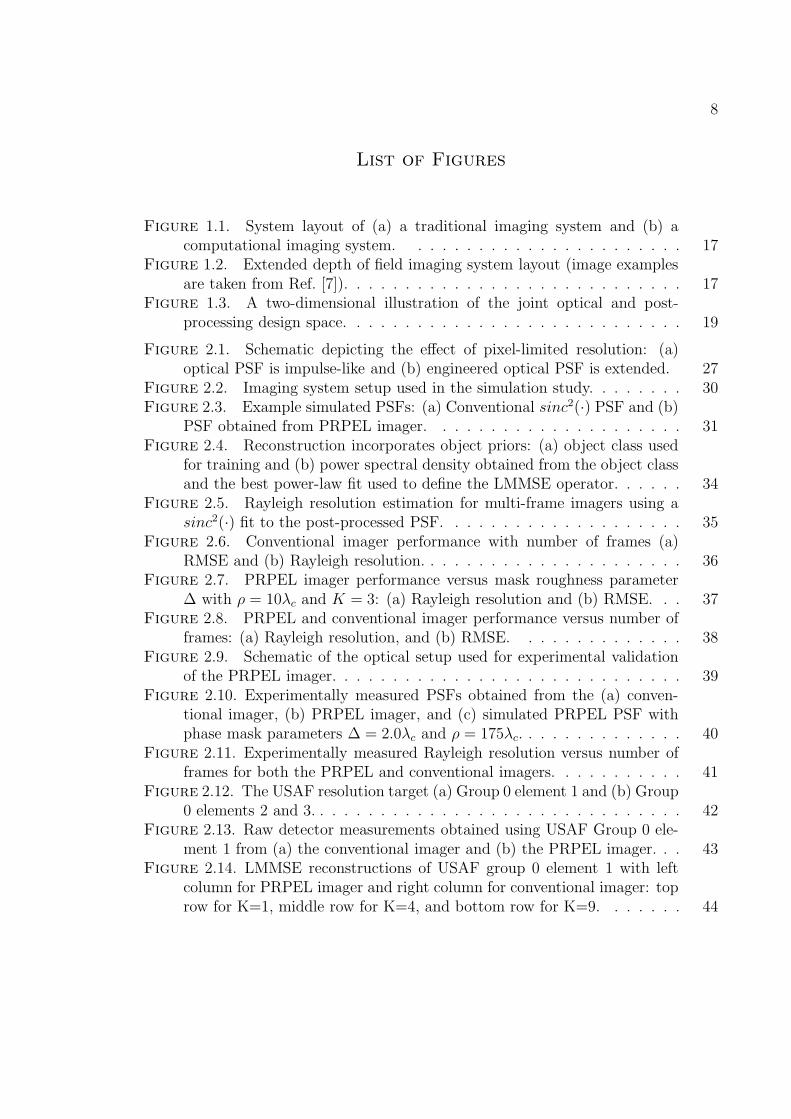
Figure 1.1. System layout of (a) a traditional imaging system and (b) acomputational imaging system. . . . . . . . . . . . . . . . . . . . . . . 17
Figure 1.2. Extended depth of field imaging system layout (image examplesare taken from Ref. [7]). . . . . . . . . . . . . . . . . . . . . . . . . . . . 17
Figure 1.3. A two-dimensional illustration of the joint optical and post-processing design space. . . . . . . . . . . . . . . . . . . . . . . . . . . . 19
Figure 2.1. Schematic depicting the effect of pixel-limited resolution: (a)optical PSF is impulse-like and (b) engineered optical PSF is extended. 27
Figure 2.2. Imaging system setup used in the simulation study. . . . . . . . 30Figure 2.3. Example simulated PSFs: (a) Conventional sinc2(·) PSF and (b)
PSF obtained from PRPEL imager. . . . . . . . . . . . . . . . . . . . . 31Figure 2.4. Reconstruction incorporates object priors: (a) object class used
for training and (b) power spectral density obtained from the object classand the best power-law fit used to define the LMMSE operator. . . . . . 34
Figure 2.5. Rayleigh resolution estimation for multi-frame imagers using asinc2(·) fit to the post-processed PSF. . . . . . . . . . . . . . . . . . . . 35
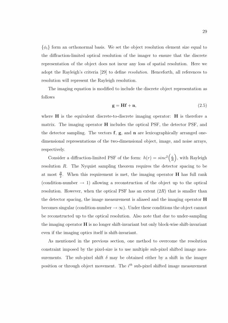
Figure 2.6. Conventional imager performance with number of frames (a)RMSE and (b) Rayleigh resolution. . . . . . . . . . . . . . . . . . . . . . 36
Figure 2.7. PRPEL imager performance versus mask roughness parameter∆ with ρ = 10λc and K = 3: (a) Rayleigh resolution and (b) RMSE. . . 37
Figure 2.8. PRPEL and conventional imager performance versus number offrames: (a) Rayleigh resolution, and (b) RMSE. . . . . . . . . . . . . . 38
Figure 2.9. Schematic of the optical setup used for experimental validationof the PRPEL imager. . . . . . . . . . . . . . . . . . . . . . . . . . . . . 39
Figure 2.10. Experimentally measured PSFs obtained from the (a) conven-tional imager, (b) PRPEL imager, and (c) simulated PRPEL PSF withphase mask parameters ∆ = 2.0λc and ρ = 175λc. . . . . . . . . . . . . . 40
Figure 2.11. Experimentally measured Rayleigh resolution versus number offrames for both the PRPEL and conventional imagers. . . . . . . . . . . 41
Figure 2.12. The USAF resolution target (a) Group 0 element 1 and (b) Group0 elements 2 and 3. . . . . . . . . . . . . . . . . . . . . . . . . . . . . . . 42
Figure 2.13. Raw detector measurements obtained using USAF Group 0 ele-ment 1 from (a) the conventional imager and (b) the PRPEL imager. . . 43
Figure 2.14. LMMSE reconstructions of USAF group 0 element 1 with leftcolumn for PRPEL imager and right column for conventional imager: toprow for K=1, middle row for K=4, and bottom row for K=9. . . . . . . 44

List of Figures—Continued
9
Figure 2.15. Horizontal line scans through the USAF target and its LMMSEreconstruction for conventional and PRPEL imagers for K=4: (a) group0 elements 1 and (b) group 0 elements 2 and 3. . . . . . . . . . . . . . . 45
Figure 2.16. LMMSE reconstructions of USAF group 0 element 2 and 3 withleft column for PRPEL imager and right column for conventional imager:top row for K=1, middle row for K=4, and bottom row for K=9. . . . . 46
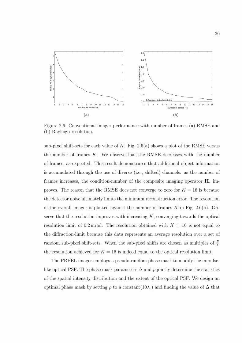
Figure 2.17. Richardson-Lucy reconstructions of USAF group 0 element 1with left column for PRPEL imager and right column for conventionalimager: top row for K=1, middle row for K=4, and bottom row for K=9. 48
Figure 2.18. Richardson-Lucy reconstructions of USAF group 0 element 2 and3 with left column for PRPEL imager and right column for conventionalimager: top row for K=1, middle row for K=4, and bottom row for K=9. 49
Figure 2.19. Horizontal line scans through the USAF target and its Richardson-Lucy reconstruction for conventional and PRPEL imagers for K=4: (a)group 0 elements 1 and (b)group 0 elements 2 and 3. . . . . . . . . . . . 50
Figure 2.20. (a) Rayleigh resolution and (b) RMSE versus number of framesfor multi-frame imagers that employ smaller pixels and lower measure-ment SNR. . . . . . . . . . . . . . . . . . . . . . . . . . . . . . . . . . . 51
Figure 2.21. The optical PSF obtained using PRPEL with both narrowband(10 nm) and broadband (150 nm) illumination. . . . . . . . . . . . . . . 52
Figure 2.22. (a) Rayleigh resolution and (b) RMSE versus number of framesfor broadband PRPEL and conventional imagers. . . . . . . . . . . . . . 53
Figure 3.1. PSF-engineered multi-aperture imaging system layout. . . . . . 57Figure 3.2. Iris examples from the training dataset. . . . . . . . . . . . . . 60Figure 3.3. Examples of (a) iris-segmentation, (b) masked iris-texture region,
(c) unwrapped iris, and (d) iris-code. . . . . . . . . . . . . . . . . . . . . 62Figure 3.4. Illustration of FRR and FAR definitions in the context of intra-
class and inter-class probability densities. . . . . . . . . . . . . . . . . . 65Figure 3.5. Optimized ZPEL imager with K = 1 (a) pupil-phase, (b) optical
PSF, and (c) optical PSF of conventional imager . . . . . . . . . . . . . 70Figure 3.6. Cross-section MTF profiles of optimized ZPEL imager with K = 1. 71Figure 3.7. Optimized ZPEL imager with K = 4: (a) pupil-phase and (b)
optical PSF. . . . . . . . . . . . . . . . . . . . . . . . . . . . . . . . . . 71Figure 3.8. Cross-section MTF profiles of optimized ZPEL imager with K = 4. 72Figure 3.9. Optimized ZPEL imager with K = 9: (a) pupil-phase and (b)
optical PSF. . . . . . . . . . . . . . . . . . . . . . . . . . . . . . . . . . 73Figure 3.10. Cross-section MTF profiles of optimized ZPEL imager with K = 9. 73Figure 3.11. Optimized ZPEL imager with K = 16: (a) pupil-phase and (b)
optical PSF. . . . . . . . . . . . . . . . . . . . . . . . . . . . . . . . . . 74
List of Figures—Continued
10
Figure 3.12. Cross-section MTF profiles of optimized ZPEL imager with K =16. . . . . . . . . . . . . . . . . . . . . . . . . . . . . . . . . . . . . . . . 74
Figure 3.13. Iris examples from the validation dataset. . . . . . . . . . . . . 76
Figure 4.1. (a) A 256 × 256 image, (b) the compressed version of image in(a) using JPEG2000, and (c) 64 × 64 image obtained by rescaling imagein (a). . . . . . . . . . . . . . . . . . . . . . . . . . . . . . . . . . . . . . 80
Figure 4.2. Block diagram of an imaging chain. . . . . . . . . . . . . . . . . 83Figure 4.3. Example scenes from the deterministic encoder. . . . . . . . . . 83Figure 4.4. Example scenes from the stochastic encoder. . . . . . . . . . . . 84Figure 4.5. (a) mmse and (b) TSI versus signal to noise ratio for the scalar
detection task. . . . . . . . . . . . . . . . . . . . . . . . . . . . . . . . . 88Figure 4.6. Illustration of stochastic encoding Cdet: (a) Target profile matrix
T and position vector ~ρ and (b) clutter profile matrix Vc and mixing
vector ~β. . . . . . . . . . . . . . . . . . . . . . . . . . . . . . . . . . . . 90Figure 4.7. Structure of T and ρ matrices for the two-class problem. . . . . 92Figure 4.8. Structure of T and Λ matrices for the joint detection/localization
problem. . . . . . . . . . . . . . . . . . . . . . . . . . . . . . . . . . . . 94Figure 4.9. Structure of T and Ω matrices for the joint classification/localization
problem. . . . . . . . . . . . . . . . . . . . . . . . . . . . . . . . . . . . 96Figure 4.10. Example scenes: (a) Tank in the middle of the scene, (b) Tank
in the top of the scene, (c) Jeep at the bottom of the scene, and (d) Jeepin the middle of the scene. . . . . . . . . . . . . . . . . . . . . . . . . . . 98
Figure 4.11. Detection task: (a) mmse versus signal to noise ratio for an idealgeometric imager and (b) TSI versus signal to noise ratio for geometricand diffraction-limited imagers. . . . . . . . . . . . . . . . . . . . . . . . 101
Figure 4.12. Scene partitioned into four regions: (a) Tank in the top left regionof the scene, (b) Tank in the top right region of the scene, (c) Tank in thebottom left region of the scene, and (d) Tank in the bottom right regionof the scene. . . . . . . . . . . . . . . . . . . . . . . . . . . . . . . . . . 103
Figure 4.13. Joint detection/localization task: (a) mmse versus signal to noiseratio for an ideal geometric imager and (b) TSI versus signal to noise ratiofor geometric and diffraction-limited imagers. . . . . . . . . . . . . . . . 104
Figure 4.14. Classification task: TSI versus signal to noise ratio for geometricand diffraction-limited imagers. . . . . . . . . . . . . . . . . . . . . . . . 106
Figure 4.15. Joint classification/localization task: TSI versus signal to noiseratio for geometric and diffraction-limited imagers. . . . . . . . . . . . . 107
Figure 4.16. Example scenes with optical blur: (a) Tank in the top of thescene, (b) Tank in the middle of the scene, (c) Jeep at the bottom of thescene, and (d) Jeep in the middle of the scene. . . . . . . . . . . . . . . 108

List of Figures—Continued
11
Figure 4.17. Block diagram of a compressive imager. . . . . . . . . . . . . . 109Figure 4.18. Detection task: TSI for PC compressive imager versus signal to
noise ratio. . . . . . . . . . . . . . . . . . . . . . . . . . . . . . . . . . . 111Figure 4.19. Joint detection/localization task: TSI for PC compressive imager
versus signal to noise ratio. . . . . . . . . . . . . . . . . . . . . . . . . . 112Figure 4.20. Detection task: TSI for MF compressive imager versus signal to
noise ratio. . . . . . . . . . . . . . . . . . . . . . . . . . . . . . . . . . . 114Figure 4.21. Joint detection/localization task: TSI for MF compressive imager
versus signal to noise ratio. . . . . . . . . . . . . . . . . . . . . . . . . . 115Figure 4.22. Example textures (a) from each of the 16 texture classes and (b)
within one of the texture class. . . . . . . . . . . . . . . . . . . . . . . . 116Figure 4.23. TSI versus signal to noise ratio at various values of defocus. . . 117Figure 4.24. TSI versus defocus at s = 10 and s = 4 for the texture classifi-
cation task. . . . . . . . . . . . . . . . . . . . . . . . . . . . . . . . . . . 118Figure 4.25. Optical PSF of conventional imager at (a) Wd = 0, (b) Wd = 3
and cubic phase-mask imager with γ = 2.0 at (c) Wd = 0, (d) Wd = 3. . 119Figure 4.26. Depth of Field and TSI versus γ parameter at s = 10. . . . . . 122Figure 4.27. TSI versus defocus at s = 10: DOF of conventional imager and
cubic phase-mask EDOF imager with optimized optical PSF. . . . . . . 122
Figure 5.1. Candidate optical architectures for compressive imaging (a) se-quential and (b) parallel. . . . . . . . . . . . . . . . . . . . . . . . . . . 126
Figure 5.2. Block diagram of a compressive imaging system. . . . . . . . . . 129Figure 5.3. Illustration of stochastic encoding C: (a) Target profile matrix T
and position vector ~ρ and (b) clutter profile matrix Vc and mixing vector~β. . . . . . . . . . . . . . . . . . . . . . . . . . . . . . . . . . . . . . . . 132
Figure 5.4. Difference mmse and mmse components versus SNR for a con-ventional imager. . . . . . . . . . . . . . . . . . . . . . . . . . . . . . . . 135
Figure 5.5. Example scenes with optical blur and noise: (a) Tank in the topof the scene, (b) Tank in the middle of the scene . . . . . . . . . . . . . 136
Figure 5.6. Example projection vectors in the PC projection basis, clockwisefrom upper left, #2,#6,#16,#31. . . . . . . . . . . . . . . . . . . . . . . 140
Figure 5.7. TSI versus SNR for PC compressive imager. . . . . . . . . . . . 141Figure 5.8. Example projection vectors in the GMF projection basis, clock-
wise from upper left, #1,#16,#32,#64. . . . . . . . . . . . . . . . . . . 143Figure 5.9. Example projection vectors in the GFD1 projection basis, clock-
wise from upper left, #1,#10,#11,#14. . . . . . . . . . . . . . . . . . . 146Figure 5.10. Projection vector in the GFD2 projection basis. . . . . . . . . . 147Figure 5.11. Example projection vectors in the IC projection basis, clockwise
from upper left, #8,#16,#22,#28. . . . . . . . . . . . . . . . . . . . . . 149

List of Figures—Continued
12
Figure 5.12. Optimized compressive imagers: TSI versus SNR for candidateCI system and conventional imager. . . . . . . . . . . . . . . . . . . . . 150
Figure 5.13. Optimal photon allocation vectors for PC compressive imager at:(a) s = 0.5 , (b) s = 5.0 , and (c) s = 20.0. . . . . . . . . . . . . . . . . . 151
Figure 5.14. Optimal photon allocation vectors for GFD1 compressive imagerat: (a) s = 0.5 , (b) s = 5.0 , and (c) s = 20.0. . . . . . . . . . . . . . . 156
Figure 5.15. Lower bound on probability of error as a function of TSI. . . . 158Figure 5.16. Comparison of probability of error obtained via Bayes’ detector
versus lower bound obtained by Fano’s inequality as a function of SNR. 159
13
Abstract
The traditional approach to imaging system design places the sole burden of image
formation on optical components. In contrast, a computational imaging system relies
on a combination of optics and post-processing to produce the final image and/or
output measurement. Therefore, the joint-optimization (JO) of the optical and the
post-processing degrees of freedom plays a critical role in the design of computa-
tional imaging systems. The JO framework also allows us to incorporate task-specific
performance measures to optimize an imaging system for a specific task. In this
dissertation, we consider the design of computational imaging systems within a JO
framework for two separate tasks: object reconstruction and iris-recognition. The
goal of these design studies is to optimize the imaging system to overcome the perfor-
mance degradations introduced by under-sampled image measurements. Within the
JO framework, we engineer the optical point spread function (PSF) of the imager,
representing the optical degrees of freedom, in conjunction with the post-processing
algorithm parameters to maximize the task performance. For the object reconstruc-
tion task, the optimized imaging system achieves a 50% improvement in resolution
and nearly 20% lower reconstruction root-mean-square-error (RMSE ) as compared to
the un-optimized imaging system. For the iris-recognition task, the optimized imaging
system achieves a 33% improvement in false rejection ratio (FRR) for a fixed alarm ra-
tio (FAR) relative to the conventional imaging system. The effect of the performance
measures like resolution, RMSE, FRR, and FAR on the optimal design highlights
the crucial role of task-specific design metrics in the JO framework. We introduce a
fundamental measure of task-specific performance known as task-specific information
(TSI), an information-theoretic measure that quantifies the information content of an
image measurement relevant to a specific task. A variety of source-models are derived
to illustrate the application of a TSI-based analysis to conventional and compressive

14
imaging (CI) systems for various tasks such as target detection and classification. A
TSI-based design and optimization framework is also developed and applied to the
design of CI systems for the task of target detection, it yields a six-fold performance
improvement over the conventional imaging system at low signal-to-noise ratios.

15
Chapter 1
Introduction
1.1. Evolution of Imaging Systems
The first imaging systems simply imaged a scene onto a screen for viewing purposes.
One of the earliest imaging devices “camera obscura,” invented in the 10th century,
relied on a pinhole and a screen to form an inverted image [1]. The next signifi-
cant step in the evolution of imaging systems was the development of photo-sensitive
material that allowed the image to be recorded for later viewing. The perfection
of photographic film gave birth to a multitude of new applications, ranging from
medical imaging using X-rays for diagnosis purposes to aerial imaging for surveil-
lance. Development of the charge-coupled device (CCD) in 1969 by George Smith
and Willard Boyle at Bell labs [2] combined with the advances in communication
theory revolutionized imaging system design and its applications. The electronic
recording of an image allowed it to be stored digitally and transmitted over long dis-
tances reliably using digital communication systems. Furthermore, with the advent of
computed-aided optical design coupled with the development of modern machining
tools and new optical materials such as plastics/polymers allowed imaging system
designs that were light-weight, low-cost, and high-performance. This led to an ex-
plosion of applications, such as medical imaging for diagnosis, military applications
involving surveillance, tracking, recognition, weapon guidance, and a host of com-
mercial imaging applications such as security, consumer photography, automotive,
aerospace, and entertainment. Advances in the semiconductor industry have allowed
the processing power of computers and embedded processors to grow at an expo-
nential rate following Moore’s law [3]. This has led to real-time implementations of

16
sophisticated image processing algorithms that can further enhance the capabilities
of digital imaging systems. The post-processing algorithms, operating on acquired
images, have been developed for a variety of tasks such as pattern-recognition in se-
curity and surveillance, image restoration, detection in medical diagnosis, estimation
in computer vision, compression of still images and video storage/transmission appli-
cations. However, due to the separate evolutionary paths of imaging system design
and image processing technology, they have been viewed as two separate processes by
imaging system designers. As a result, there has been a disconnect between the imag-
ing system design and the post-processing algorithm design. Recently, this disconnect
has been addressed with the emergence of a new imaging system paradigm known
as computational imaging [4, 5, 6]. Computational imaging offers several advantages
over traditional imaging techniques, especially when dealing with specific tasks. This
dissertation investigates the task-specific aspects of design methodologies for compu-
tational imaging system design. Before discussing the specific contributions of this
dissertation we begin by defining computational imaging and outlining its various
benefits relative to traditional imaging.
1.2. Computational Imaging and Task-specific Design
In a traditional imaging system, the optics has the sole burden of the image formation.
The post-processing algorithm, which is not an essential part of the imaging system,
operates on the image measurement to extract the desired information. Note that the
optics and the post-processing algorithms are designed separately. Fig. 1.1(a) shows
the architecture of a traditional imaging system. In contrast, a computational imaging
system involves the use of both a front-end optical system and a post-processing
algorithm in the image formation process. As shown in Fig. 1.1(b), the post-processing
algorithm forms an integral part of the overall imaging system design. Here the
front-end optics does not yield the final image directly but instead relies on the
17
Object
Detector array
Image
Imaging optics
Output dataalgorithm
Post−processing
(a)
Object
Detector arrayEncoded optics
Intermediate image Final image/output data
Post−processingalgorithm
(b)
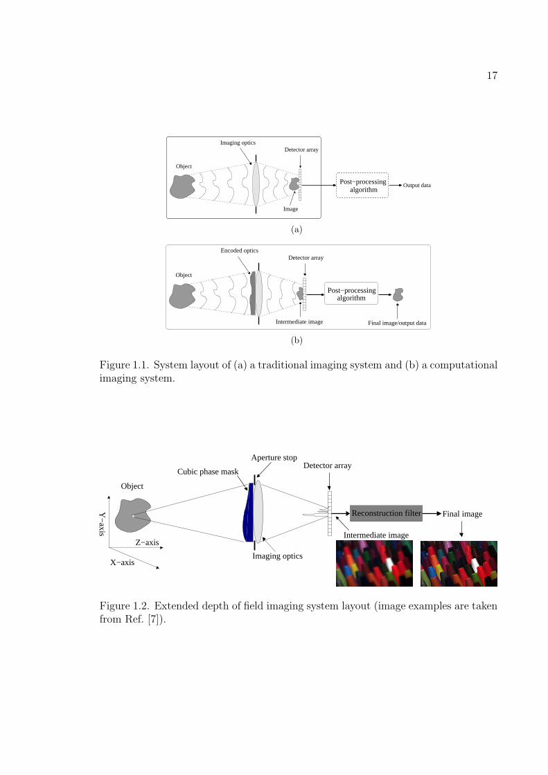
Figure 1.1. System layout of (a) a traditional imaging system and (b) a computationalimaging system.
Cubic phase mask
Imaging optics
Aperture stopDetector array
Intermediate image
Reconstruction filter
Z−axis
X−axis
Y−
axis
Object
Final image
Figure 1.2. Extended depth of field imaging system layout (image examples are takenfrom Ref. [7]).

18
post-processing sub-system to form the image. The extended depth of field (EDOF)
imaging system, described in Ref. [4], is an example of a computational imaging
system. Fig. 1.2 shows the system layout of this EDOF imaging system. Note that
it consists of a front-end optical system to form an intermediate image on the sensor
array that is subsequently processed by an image reconstruction algorithm to yield
the final focused image. The EDOF is achieved by modifying a traditional optical
imaging system with the addition of a cubic-phase mask in the aperture stop. The
resulting optical point spread function (PSF) has a larger support compared to a
traditional PSF and therefore, the optical image formed on the sensor array appears
to be blurred. However, as the optical PSF is invariant over an extended range of
object distances, a simple reconstruction filter can be used in the post-processing step
to form the final image that is focused throughout an extended object volume. This
imaging system demonstrates the potential of the computational imaging paradigm to
yield designs with novel capabilities, like EDOF, that simply could not be achieved by
a traditional imaging system without significant performance trade-offs. Nevertheless,
it is important to recognize that this EDOF imaging system does not fully exploit
the capabilities of the computational imaging paradigm.
The true potential of computational imaging can only be realized via a joint-
optimization of the optical and the post-processing degrees of freedom. The joint
design methodology yields a larger and richer design space for the designer. In order
to understand this advantage let us examine the multi-dimensional design space de-
picted in Fig. 1.3, the optical design parameters are represented on the vertical axis
and the post-processing design parameters are shown on the horizontal axis. Note
that the traditional approach constrains the designer to a relatively small design sub-
space, outlined in brown and green. The region outlined in brown represents a design
sub-space resulting from optimization of only optical parameters without any con-
sideration to the degrees of freedom available in the post-processing domain. In the
traditional design methodology, the optical design is followed by the optimization of

19
Post−processing domain parameters
Op
tica
l do
ma
in p
ara
me
ters
MinimaMaxima
Optical design sub−space
Post−processing design sub−space
Global optima
Joint design space
Figure 1.3. A two-dimensional illustration of the joint optical and post-processingdesign space.
post-processing parameters, represented by the sub-space in the green region. This
approach does not guarantee an overall optimal system design and it usually leads to
a sub-optimal system performance. In contrast, the joint-optimization design method
combines the degrees of freedom available from the optical and the post-processing do-
mains expanding the design space to a larger volume, represented by the red outlined
region. This larger design space encompasses potential designs that offer benefits
such as lower system cost, reduced complexity, improved yields and perhaps most
importantly optimal/near-optimal system performance.
Another key aspect of the joint design methodology is that it inherently supports
a task-specific approach to imaging system design. To support this assertion let us
consider an example of imaging system design for a classification task. The traditional
design approach would involve: 1) design an optical imaging system to maximize the
fidelity of the output image measurement and 2) design a classification algorithm that
operates on the image measurement and minimizes the probability of misclassifica-

20
tion. Note that in this approach the optical imaging system and the classification
algorithm are designed separately (and sequentially). Typically, a classification al-
gorithm involves two steps: the feature extraction step and the classification step.
In the feature extraction step, the original high-dimensional image measurement is
transformed (compressed) into a low-dimensional data vector that is referred to as
a feature vector. This dimensionality reduction step effectively lowers the computa-
tional complexity of the subsequent classification step. Acquiring a high-dimensional
image measurement and subsequently reducing it to a low-dimensional feature clearly
represents an inefficient data measurement process and a poor utilization of optical
design resources. Thus, the traditional approach results in an imaging system design
with sub-optimal performance for the classification task. Alternatively, a more logi-
cal approach would suggest an optical imaging system design that directly measures
the optimal low-dimensional feature(s) for post-processing such that it maximizes the
task performance, within the system constraints. This approach yields a computa-
tional imaging system design that offers two main advantages: a) a direct feature
measurement yields a higher measurement signal to noise ratio (SNR) and b) the
number of detectors required is significantly reduced. The high measurement SNR
directly translates into improved system performance. This type of imaging system,
referred to as a feature-specific imager (FSI) or a compressive imager, is an exam-
ple of a computational imaging system [6]. This example clearly illustrates that the
computational imaging paradigm supports and enables a task-specific approach to
imaging system design.
1.3. Main Contributions
The task-specific approach to computational imaging system design is an emerging
area of research. Barrett et al. have conducted an extensive task-based analysis of
imaging systems for detection and classification tasks in the area of medical imag-

21
ing [8, 9, 10]. Their focus has been primarily on the performance of ideal Bayesian
observers and human observers. However, the application of the task-specific ap-
proach within a joint-optimization design framework is a relatively unexplored area.
In this dissertation, we apply a task-specific approach to maximize the performance
of a computational imaging system for a given task within a joint-optimization design
framework. We consider two separate example tasks in this work: a reconstruction
task and a classification task. In each case, the computational imaging system is
optimized to maximize the task performance as measured by a task-specific metric.
For example, the reconstruction task employs the traditional root mean square error
(RMSE) and resolution metrics to quantify the quality of the reconstructed images.
In the case of the classification task, false rejection ratio (FRR) and false alarm ra-
tio (FAR) statistics are used as task-specific metrics to evaluate the overall system
performance. In addition to the two design studies, a novel information theoretic task-
specific metric is also derived. A formal design framework based on this task-specific
metric is developed and applied to the design of a compressive imaging system for the
task of target detection. More specifically, the main contributions of this dissertation
work are as follows:
1. The application of the optical PSF engineering method to optimize the imaging
system performance for a specific task is considered. This task-specific method
is first applied to a reconstruction task to overcome the distortions introduced by
the detector under-sampling in the sensor array. Simulation results show nearly
a 20% improvement in RMSE for the optimized imaging system design relative
to the conventional imaging system. The optical PSF engineering method is
also successfully applied to the design of an iris-recognition imaging system
to minimize the impact of detector under-sampling on the overall performance.
The optimized iris-recognition imaging system design achieves a 33% lower FRR
compared to the conventional imaging system design.

22
2. Development a formal task-specific framework for computational imaging sys-
tem design based on a novel information theoretic task-specific metric. This
metric, known as task-specific information (TSI), quantifies the information
content of an imaging system measurement relevant to a specific task. The
TSI metric can also be used to derive an upper-bound on the performance of
any post-processing algorithm for a specific task. Therefore, within the pro-
posed design framework, the TSI metric can be used improve the upper-bound
on imaging system performance thereby allowing the designer to optimize the
imaging system for a particular task. The utility of the TSI metric is investi-
gated for a variety of target detection and classification tasks. The application
of the TSI-based design framework to extend the depth of field of an imager by
optical PSF engineering is also considered.
3. The TSI-based design framework is used to design several compressive imaging
systems for a target detection task. The resulting optimized imaging system
designs shows a significant performance improvement over the un-optimized
imaging designs.
1.4. Dissertation Organization
The rest of the dissertation is organized as follows:
• Chapter 2 presents the application of the optical PSF engineering method,
within a multi-aperture imaging architecture, to overcome the distortions due
to under-sampling in the detector array. The reconstruction task is considered
in this study. RMSE and resolution are used as task-specific metrics during
the imaging system optimization process. In the simulation study, the opti-
mized imaging system designs show significant improvement, both in terms of
RMSE and resolution metrics, compared to imaging system with a traditional

23
diffraction-limited PSF. The experimental results support the performance im-
provements predicted by the simulation study.
• The task of iris-recognition, in the presence of detector under-sampling, is con-
sidered in Chapter 3. A multi-aperture imaging system in conjunction with
optical PSF engineering is employed to optimize the overall performance of the
imaging system. The task-specific design framework employs the FAR and FRR
metrics to quantify the imaging system performance in this study. The simula-
tion results show a substantial improvement in iris-recognition performance as
a result of PSF optimization compared to the design that employs a traditional
optical PSF.
• As emphasized by the design studies described in Chapter 2 and Chapter 3, the
performance metric plays a crucial role in the task-specific approach to imaging
system design. In Chapter 4, the notion of task-specfic information is introduced
as an objective metric for task-specfic design. TSI is an information theoretic
metric that is derived using the recently discovered relationship between esti-
mation theory and mutual-information. This metric is applied to a variety of
detection and classification tasks to demonstrate its utility for task-specific per-
formance evaluation. A brief analysis of a TSI-based optical PSF engineering
approach for extending the depth of field of an imager is also presented in the
context of a texture-classification task.
• Chapter 5 presents a formal task-specific design framework that utilizes the
TSI metric to optimize a compressive imaging system for a target detection
task. The optimized imaging system designs deliver substantial performance
improvement over the conventional design. The implementation issues regarding
compressive imaging systems and the computational complexity associated with
the TSI-based design framework are also discussed.

24
• Chapter 6 draws conclusions from the various aspects of the task-specifc ap-
proach investigated in this dissertation and provides direction for future work
relevant to the further development of the joint-optimization design framework
for computational imaging systems.

25
Chapter 2
Optical PSF Engineering: Object
Reconstruction Task
The optical PSF represents a degree of freedom that can be exploited to optimize
an imaging system for a specific task. In a digital imaging system, the detector
can limit the overall resolution when the optical PSF is smaller than the extent of
the detector, leading to under-sampling or aliasing. In this chapter, we apply the
optical PSF engineering method to improve the overall system resolution beyond
the detector-limit and also increase the object reconstruction fidelity in such under-
sampled imaging systems.
2.1. Introduction
In a traditional (i.e. film-based) design paradigm the optical PSF is typically viewed
as the resolution-limiting element and therefore, optical designers strive for an impulse-
like PSF. Digital imagers however, employ photodetectors that are sometimes large
relative to the extent of the optical PSF and in such cases the resulting pixel-blur
and/or aliasing can become the dominant distortion limiting overall imager perfor-
mance. This is illustrated by Fig. 2.1(a). This figure is a one-dimensional depiction
of the image formed by a traditional camera when two point objects are separated
by a sub-pixel distance. We see that the resulting impulse-like PSFs are imaged onto
essentially the same pixel leading to spatial ambiguity and hence a loss of resolution.
In such an imager the resolution is said to be pixel-limited [11].
The effect depicted in Fig. 2.1(a) may also be understood by noting that the
detector array under-samples the image and therefore, introduces aliasing. The gen-

26
eralized sampling theorem by Papoulis [12] provides a mechanism through which this
aliasing distortion can be mitigated. The theorem states that a bandlimited signal
(−Ω ≤ ω ≤ Ω) can be completely/perfectly reconstructed from the sampled outputs
of R non-redundant (i.e., diverse) linear channels, each of which employs a sample rate
of 2ΩR
(i.e., each of the R signals is under-sampled at 1R
the Nyquist rate). This theo-
rem suggests that the aliasing distortion can be reduced by combining multiple under-
sampled/low-resolution images to obtain a high-resolution image. A detailed descrip-
tion of this technique can be found in Borman [13]. This approach has been used by
several researchers in the image processing community [11, 14, 15, 16, 17, 18] and was
recently adopted for use in the TOMBO (Thin observing module with bounded optics)
imaging architecture [19, 20]. The TOMBO system was designed to simultaneously
acquire multiple low-resolution images of an object through multiple lenslets in an
integrated aperture. The resulting collection of low-resolution measurements is then
processed to yield a high-resolution image. Within the TOMBO system the multiple
non-redundant images were obtained via a diverse set of sub-pixel shifts. The use of
other forms of diversity including magnification, rotation, and defocus has also been
considered [21]. However, it is important to note that these methods of obtaining
measurement diversity do not fully exploit the optical degrees of freedom available to
the designer. The approach described in this chapter will utilize PSF engineering in
order to obtain additional diversity from a set of sub-pixel shifted measurements.
The optical PSF of a digital imager may be viewed as a mechanism for encoding
object information so as to better tolerate distortions introduced by the detector ar-
ray. From this viewpoint an impulse-like optical PSF may be sub-optimal [22, 23].
To support this assertion let us consider the scenario depicted in Fig. 2.1(b), it shows
an image of two point objects formed using a non-impulse-like PSF. The two point
objects are displaced by the same amount as in Fig. 2.1(a). We see that the use of
an extended PSF enables the extraction of sub-pixel position information from the
sampled detector outputs. For example, a simple correlation-based processor [24] can
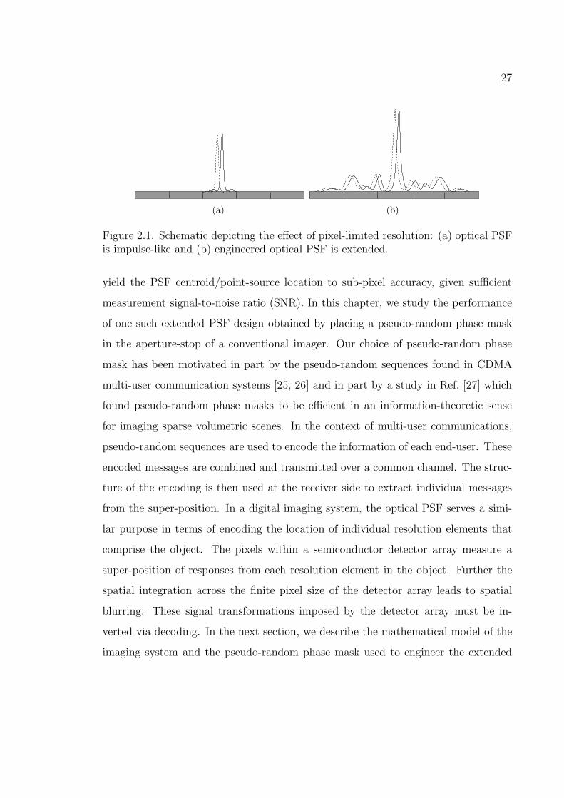
27
(a) (b)
Figure 2.1. Schematic depicting the effect of pixel-limited resolution: (a) optical PSFis impulse-like and (b) engineered optical PSF is extended.
yield the PSF centroid/point-source location to sub-pixel accuracy, given sufficient
measurement signal-to-noise ratio (SNR). In this chapter, we study the performance
of one such extended PSF design obtained by placing a pseudo-random phase mask
in the aperture-stop of a conventional imager. Our choice of pseudo-random phase
mask has been motivated in part by the pseudo-random sequences found in CDMA
multi-user communication systems [25, 26] and in part by a study in Ref. [27] which
found pseudo-random phase masks to be efficient in an information-theoretic sense
for imaging sparse volumetric scenes. In the context of multi-user communications,
pseudo-random sequences are used to encode the information of each end-user. These
encoded messages are combined and transmitted over a common channel. The struc-
ture of the encoding is then used at the receiver side to extract individual messages
from the super-position. In a digital imaging system, the optical PSF serves a simi-
lar purpose in terms of encoding the location of individual resolution elements that
comprise the object. The pixels within a semiconductor detector array measure a
super-position of responses from each resolution element in the object. Further the
spatial integration across the finite pixel size of the detector array leads to spatial
blurring. These signal transformations imposed by the detector array must be in-
verted via decoding. In the next section, we describe the mathematical model of the
imaging system and the pseudo-random phase mask used to engineer the extended

28
optical PSF.
2.2. Imaging System Model
Consider a linear model of a digital imaging system. Mathematically, we can represent
the system as
g = Hcdfc + n, (2.1)
where fc is the continuous object, g is the detector-array measurement vector, Hcd
is the continuous-to-discrete imaging operator and n is additive measurement noise
vector. For simulation purposes we use a discrete representation f of the continuous
object fc. This discrete representation f can be obtained from fc as follows [28]
fi =
∫
S∩Φi
fc(~r)φi(~r)dr2, (2.2)
where S is the object support, φi is an analysis basis set, Φi is the support of
ith basis function φi and fi is the ith element of the object vector f . Note that we
obtain an approximation fa of the original continuous object fc from its discrete
representation f as follows [28]
fa(~r) =
N∑
i=1
fi · ψi(~r), (2.3)
where N is the dimension of the discrete object vector and ψi is a synthesis basis
set which can be chosen to be the same as the analysis basis set φi. Here we use the
pixel function to construct our analysis and synthesis basis sets. The pixel function
is defined as
φi(r) =1
Ωrrect
(r − iΩr
Ωr
)(2.4)
and
∫
Φi∩Φj
φi(r)φj(r)dr2 = δij ,
where 2Ωr is the size of the resolution element in the continuous object that can
be accurately represented by this choice of basis set. Note that the pixel functions
29
φi form an orthonormal basis. We set the object resolution element size equal to
the diffraction-limited optical resolution of the imager to ensure that the discrete
representation of the object does not incur any loss of spatial resolution. Here we
adopt the Rayleigh’s criteria [29] to define resolution. Henceforth, all references to
resolution will represent the Rayleigh resolution.
The imaging equation is modified to include the discrete object representation as
follows
g = Hf + n, (2.5)
where H is the equivalent discrete-to-discrete imaging operator: H is therefore a
matrix. The imaging operator H includes the optical PSF, the detector PSF, and
the detector sampling. The vectors f , g, and n are lexicographically arranged one-
dimensional representations of the two-dimensional object, image, and noise arrays,
respectively.
Consider a diffraction-limited PSF of the form: h(r) = sinc2(
rR
), with Rayleigh
resolution R. The Nyquist sampling theorem requires the detector spacing to be
at most R2. When this requirement is met, the imaging operator H has full rank
(condition-number → 1) allowing a reconstruction of the object up to the optical
resolution. However, when the optical PSF has an extent (2R) that is smaller than
the detector spacing, the image measurement is aliased and the imaging operator H
becomes singular (condition-number → ∞). Under these conditions the object cannot
be reconstructed up to the optical resolution. Also note that due to under-sampling
the imaging operator H is no longer shift-invariant but only block-wise shift-invariant
even if the imaging optics itself is shift-invariant.
As mentioned in the previous section, one method to overcome the resolution
constraint imposed by the pixel-size is to use multiple sub-pixel shifted image mea-
surements. The sub-pixel shift δ may be obtained either by a shift in the imager
position or through object movement. The ith sub-pixel shifted image measurement

30
X−axis
Y−
axis
Z−axis
Det
ecto
r−ar
ray Pseudo−random phase mask
Lens system
Apertute stop
Object
Figure 2.2. Imaging system setup used in the simulation study.
gi with shift δi can be represented as
gi = Hif + ni, (2.6)
where Hi represents the imaging operator associated with the sub-pixel shift δi.
For a set of K such measurements we can write the composite image measure-
ment by concatenating the individual vectors as, g =g1 g2 · · ·gK
and similarly
n =n1 n2 · · ·nK
. The overall multi-frame composite imaging system can be ex-
pressed as
g = Hcf + n, (2.7)
where Hc is the composite imaging operator. By combining several sub-pixel shifted
image measurements, the condition number of the composite imaging operator Hc
can be progressively improved and the overall resolution can be increased towards
the optical resolution limit. Ideally, the sub-pixel shifts should be chosen in multiples
of DK
so as to minimize the condition-number of the forward imaging operator Hc,
where D is the detector spacing [30].
We are interested in designing an extended optical PSF for use within the sub-pixel
shifting framework. The use of an extended optical PSF can improve the condition-
number of the imaging operator Hc. We consider an extended optical PSF obtained
by placing a pseudo-random phase mask in the aperture-stop of a conventional imager,
as shown in Fig. 2.2. For simulation purposes the aperture-stop is defined on a discrete
spatial grid. Therefore, the pseudo-random phase mask is represented by an array,

31
−15 −10 −5 0 5 10 150
2
4
6
8
10
12
14
Spatial dimension [µm]
Am
plitu
de
x10−3
(a)
−15 −10 −5 0 5 10 150
0.2
0.4
0.6
0.8
1
1.2
1.4
1.6
x 10−3
Spatial dimension [µm]
Am
plitu
de
(b)
Figure 2.3. Example simulated PSFs: (a) Conventional sinc2(·) PSF and (b) PSFobtained from PRPEL imager.
each element of which corresponds to the phase at given a position on the discrete
spatial grid. The pseudo-random phase mask is synthesized in two steps: (1) generate
a set of identical independently distributed random numbers distributed uniformly
on the interval [0,∆] to populate the phase array and (2) convolve this phase array
with a Gaussian filter kernel which is a Gaussian function with standard-deviation
ρ, sampled on the discrete spatial grid. The resulting set of random numbers define
the phase distribution Φ(r) of the pseudo-random phase mask. The phase mask is
thus a realization of a spatial Gaussian random process which is parameterized by
its roughness ∆ and correlation length ρ. The auto-correlation function of this phase
distribution is given by
RΦΦ(r) =∆
12
2
exp
[− r2
4ρ2
]. (2.8)
The incoherent PSF is related to the phase-mask profile Φ(r) as follows [28]
psf(r) =Ac
(λf)4
∣∣∣∣Tpupil
(− r
λf
)∣∣∣∣2
, (2.9)
Tpupil(ω) = F exp[j2π(nr − 1)Φ(r)/λ]tap(r) , (2.10)
where Ac is normalization constant with units of area, nr is the refractive index of
the lens, f is the back focal length, tap(r) is the aperture function and F denotes the
forward Fourier transform operator.

32
Fig. 2.3(a) shows a simulated impulse-like PSF and Fig. 2.3(b) an extended PSF
resulting from simulating a pseudo-random phase mask with parameters ∆ = 1.5λc
and ρ = 10λc, where λc is the operating center wavelength. Here we set λc =550 nm
and the imager F/# = 1.8. Assuming a detector size of 7.5µm, the support of
extended PSF extends over roughly six detectors, in contrast with a sub-pixel extent
of 2µm for the impulse-like PSF. The extended PSF will therefore accomplish the
desired encoding; however, it will do so at the cost of measurement SNR. Because the
extended PSF is spread over several pixels, its photon count per detector is lower than
that for the impulse-like PSF for a point-like object. Assuming a constant detector
noise, the measurement SNR per detector for the extended PSF is thus lower than
that of the impulse-like PSF. For more general objects, the extended PSF results in
a reduced contrast image with a commensurate SNR reduction, though smaller than
for point-like objects. In the next section, we present a simulation study to quantify
the tradeoff between the overall imaging resolution and the SNR for two candidate
imagers that use multiple sub-pixel shifted measurements: (a) the conventional imager
and (b) the pseudo-random phase enhanced lens (PRPEL) imager.
2.3. Simulation results
For the purposes of the simulation study, we consider only one-dimensional objects
and image measurements. The target imaging system has a modest specification with
an angular resolution of 0.2mrad and an angular field of view(FOV) of 0.1 rad. The
conventional imager uses a lens of F/# = 1.8 and back focal length 5mm. We assume
that the lens is diffraction-limited and the optical PSF is shift-invariant. The detector
array in the image plane has a pixel size of 7.5µm with a full-well capacity (FWC) of
45000 electrons and a 100% fill factor. We further assume that the imager’s spectral
bandwidth is limited to 10 nm centered at λc =550 nm. For the PRPEL imager the
only modification is that the lens is followed by a pseudo-random phase mask with

33
parameters ∆ and ρ.
We assume a shot-noise limited SNR=46dB (20 log10
√FWC) given by the FWC
of the detector element. The shot-noise is modeled as equivalent AWGN with variance
σ2 = FWC. The under-sampling factor for this imager is F = 15. This implies that
for an object vector f of size N×1 the resulting image measurement vector gi is of size
M × 1 where M = NF
. For the target imager, these values are N = 512 and M = 34.
Note that the block-wise shift-invariant imaging operator Hc is of size KM ×N .
To improve the overall imager performance we consider multiple sub-pixel shifted
image measurements or frames. These frames result from moving the imager with
respect to the object by a sub-pixel distance δi. Here it is important to constrain
the number of photons per frame to ensure a fair comparison among imagers using
multiple frames. We have two options: (a) assume that each imager has access to
the same finite number of photons and (b) assume that each frame of each imager
has access to the same finite number of photons. Option (b) may be physical under
certain conditions; however, the results that are obtained will be unable to distinguish
between improvements arising from frame diversity versus improvements arising from
increased SNR. We therefore utilize option (a) because it is the only option that
allows us to study how best to use fixed photon resources. As a result, the photon
count for each frame is normalized to FK
in this simulation study.
The inversion of the composite imaging Eq. (2.7), is based on the optimal linear-
minimum-mean-squared-error (LMMSE) operator W. The resulting object estimate
is given by
f = Wg, (2.11)
where W is defined as [31]
W = RfHT
c(HcRfH
T
c+ Rn)−1. (2.12)
Rf is the auto-correlation matrix for the object vector f and Rn is the auto-correlation
matrix of the noise vector n. Because the composite imaging operator Hc is not shift-

34
(a)
20 40 60 80 100 120 140 160
−80
−70
−60
−50
−40
−30
−20
−10
0
Angular frequency [cycles/degree]
Log
pow
er s
pect
ral d
ensi
ty
Burg estimatePower law η=1.0Power law η=1.4Power law η=2.0
(b)
Figure 2.4. Reconstruction incorporates object priors: (a) object class used for train-ing and (b) power spectral density obtained from the object class and the best power-law fit used to define the LMMSE operator.
invariant the LMMSE solution does not reduce to the well-known Wiener filter. The
noise auto-correlation matrix reduces to a diagonal matrix under the assumption of
independent and identically distributed (i.i.d.) noise and therefore, can be written as
Rn = σ2I. The object auto-correlation matrix Rf incorporates object prior knowl-
edge within the reconstruction process as a regularizing term. Here we obtain the
object auto-correlation matrix from a power-law power spectral density (PSD): 1fη ,
that serves as a good model for natural images [32, 33, 34]. A power-law PSD was
computed to model the class of 10 objects shown in Fig. 2.4(a) chosen to represent
a wide variety of scenes (rows and columns of these scenes are used as 1D objects).
Fig. 2.4(b) shows several power law PSDs plotted along with the PSD obtained using
Burg’s method [35] on 3 objects chosen from the set in Fig. 2.4(a). The power-law
PSD(η = 1.4) is used to model the PSD of the object class as it is applicable to wider
range of natural images compared to PSD models such as Burg’s that are obtained
for a specific set of objects. The value of power-law PSD parameter η was obtained
by a least-squares fit to the Burg’s PSD estimate.
In order to quantify the performance of both the PRPEL and the conventional

35
−2 −1 0 1 2
0
0.1
0.2
0.3
0.4
0.5
0.6
0.7
0.8
0.9
1
Angular dimension [mrad]
Am
plitu
de
Post−processed PSF
Fitted sinc2(.) PSF
Estimated resolution=0.4mrad
Figure 2.5. Rayleigh resolution estimation for multi-frame imagers using a sinc2(·)fit to the post-processed PSF.
imaging systems we employ two metrics: (a) Rayleigh resolution and (b) normalized
root-mean-square-error (RMSE). The Rayleigh resolution of a composite multi-frame
imager is found by using a point-source object and applying the LMMSE operator to
the K image frames. The resulting point-source reconstruction represents the overall
PSF of the computational imager. A least-squares fit of a diffraction-limited sinc2(·)PSF to the overall imager PSF is used to obtain the resolution estimate. Fig. 2.5
illustrates this resolution estimation method with an example of a post-processed PSF
and the associated sinc2(·) fit. The second imager performance metric uses RMSE
to quantify the quality of a reconstructed object. The RMSE metric is defined as,
RMSE =
√〈||f − f ||2〉
255× 100%, (2.13)
where 255 is the peak object pixel value. Here, the expectation 〈·〉 is taken over both
the object and the noise ensembles. We have used all columns and rows of the 2D
objects shown in Fig. 2.4(a) to form a set of 1D objects for computing the RMSE
metric in the simulation study.
First, we consider the conventional imager. The sub-pixel shift for each frame
is chosen randomly. The performance metrics are computed and averaged over 30
36
1 2 3 4 5 6 7 8 9 10 11 12 13 14 15 16
2
3
4
5
6
7
Number of frames − K
RM
SE
[% o
f dyn
amic
ran
ge]
(a)
1 2 3 4 5 6 7 8 9 10 11 12 13 14 15 16
0.2
0.4
0.6
0.8
1
1.2
1.4
1.6
Number of frames − K
Ang
ular
res
olut
ion
[mra
d]
Diffraction−limited resolution
(b)
Figure 2.6. Conventional imager performance with number of frames (a) RMSE and(b) Rayleigh resolution.
sub-pixel shift-sets for each value of K. Fig. 2.6(a) shows a plot of the RMSE versus
the number of frames K. We observe that the RMSE decreases with the number
of frames, as expected. This result demonstrates that additional object information
is accumulated through the use of diverse (i.e., shifted) channels: as the number of
frames increases, the condition-number of the composite imaging operator Hc im-
proves. The reason that the RMSE does not converge to zero for K = 16 is because
the detector noise ultimately limits the minimum reconstruction error. The resolution
of the overall imager is plotted against the number of frames K in Fig. 2.6(b). Ob-
serve that the resolution improves with increasing K, converging towards the optical
resolution limit of 0.2mrad. The resolution obtained with K = 16 is not equal to
the diffraction-limit because this data represents an average resolution over a set of
random sub-pixel shift-sets. When the sub-pixel shifts are chosen as multiples of DF
the resolution achieved for K = 16 is indeed equal to the optical resolution limit.
The PRPEL imager employs a pseudo-random phase mask to modify the impulse-
like optical PSF. The phase mask parameters ∆ and ρ jointly determine the statistics
of the spatial intensity distribution and the extent of the optical PSF. We design an
optimal phase mask by setting ρ to a constant(10λc) and finding the value of ∆ that

37
1 2 3 4 5 6 7 8 9
0.35
0.4
0.45
0.5
0.55
0.6
0.65
0.7
Mask roughness − ∆ [λ], ρ=10λ
Ang
ular
res
olut
ion
[mra
d]
0.5 1 1.5 2 2.5 3 3.5 4 4.5 5 5.5 6
3.8
4
4.2
4.4
4.6
4.8
5
Mask roughness − ∆[λ] ρ=10[λ]
RM
SE
[% o
f dyn
amic
ran
ge]
Figure 2.7. PRPEL imager performance versus mask roughness parameter ∆ withρ = 10λc and K = 3: (a) Rayleigh resolution and (b) RMSE.
maximizes the imager performance for a given K. Fig. 2.7(a) presents representative
data quantifying imager resolution as a function of ∆ with ρ = 10λc and K = 3. This
plot shows the fundamental tradeoff between the condition number of the imaging
operator and the SNR cost. Note that for small values of ∆ the PSF is impulse-like.
As the value of ∆ increases the PSF becomes more diffuse as shown in Fig. 2.3(b).
This results in an improvement in condition number; however, as the PSF becomes
more diffuse the photon-count per detector decreases resulting in an overall decrease in
measurement SNR. Fig. 2.7(a) shows that optimal resolution is achieved for ∆ = 7λc.
Fig. 2.7(b) demonstrates a similar trend in RMSE versus ∆ with ρ = 10λc and K = 3.
The optimal value of ∆ under the RMSE metric is ∆ = 1.5λc. Note that the optimal
values of ∆ are different for the resolution and RMSE metrics. The resolution of an
imager is determined by its spatial frequency response alone; whereas, the RMSE is
dependent on the spatial frequency response as well as the object statistics. Therefore,
the value of ∆ that maximizes the resolution metric may result in an imager with a
particular spatial frequency response that may not achieve the minimum RMSE given
the object statistics and detector noise. All the subsequent results for the PRPEL
imager are obtained for the optimal value of ∆ which will therefore be a function of

38
1 2 3 4 5 6 7 8 9 10 11 12 13 14 15 1616
0.2
0.4
0.6
0.8
1
1.2
1.4
1.6
Number of frames − K
Ang
ular
res
olut
ion
[mra
d]
Lens imagerPRPEL imager
Diffraction−limited resolution
1 2 3 4 5 6 7 8 9 10 11 12 13 14 15 16161
2
3
4
5
6
7
8
Number of Frames − K
RM
SE
[% o
f dyn
amic
ran
ge]
Lens imagerPRPEL imager
Figure 2.8. PRPEL and conventional imager performance versus number of frames:(a) Rayleigh resolution, and (b) RMSE.
K, σ and the metric (RMSE or resolution).
Fig. 2.8(a) presents the resolution performance of both the PRPEL and the con-
ventional imagers as a function of the number of frames K. We note that the PRPEL
imager converges faster than the conventional imager. A resolution of 0.3mrad is
achieved with only K = 4 by the PRPEL imager in contrast with K = 12 for the
conventional imager. A plot comparing the RMSE performance of the two imagers
is shown in Fig. 2.8(b). We note that the PRPEL imager is consistently superior to
the conventional imager. For K = 4 the PRPEL imager achieves an RMSE of 3.5%
as compared with RMSE of 4.3% for the conventional imager.
2.4. Experimental results
An experimental demonstration of the PRPEL imager was undertaken in order to
validate the performance improvements predicted by simulation. Fig. 2.9 shows the
experimental setup along with the relevant physical dimensions. A Santa Barbara
Instrument Group ST2000XM CCD was used as the detector array. The CCD consists
of a 1600 × 1200 detector array, with a detector size of 7.4µm, 100% fill factor and
a FWC of 45000 electrons. The detector output from the CCD is quantized with a

39
X−axis
Y−
axis
FOV
16mm
SB
IG C
CD
arr
ay
Fiber−tip
7.4µ
m
m21
0µ
m210µ
Fujinon Lens Ape
rtur
e =
20m
m Diffuser(phase mask)Zoom lens(2.5x)
540mm
Figure 2.9. Schematic of the optical setup used for experimental validation of thePRPEL imager.
16 bit analog-digital convertor yielding a dynamic range of [0− 64000] digital counts.
During the experiment the CCD is cooled to −10 C, to minimize electronic noise.
The experimental setup uses a Fujinon’s CF16HA-1 TV lens operated at F/#=4.0. A
circular holographic diffuser from Physical Optical Corporation is used as a pseudo-
random phase mask. The divergence angle(full-width half-maximum) of the diffuser
is 0.1. A zoom lens with magnification 2.5x is used to decrease the divergence angle
of the diffuser. The actual phase statistics of the diffuser are not disclosed by the
manufacturer. Therefore, to relate the physical diffuser to the pseudo-random phase
mask model we compute phase mask parameters ∆ and ρ that yield a PSF similar
to the one produced by the physical diffuser. The phase mask parameters ∆ = 2.0λc
and ρ = 175λc yield the PSF shown in Fig. 2.10(c). Comparing this PSF to the
PRPEL experimental PSF shown in Fig. 2.10(b), we note that they are similar in
appearance. This comparison although qualitative suggests that the physical diffuser
might possess statistics similar to the pseudo-random phase mask model described
here.
The Rayleigh resolution of the conventional optical PSF was estimated to be 5µm
or 0.31mrad. This yields an under-sampling factor of F = 3 along each direction.
This implies that a total of F 2 = 9 frames are required to achieve the full optical

40
[mrad]
[mra
d]
−3 −2 −1 0 1 2 3
−3
−2
−1
0
1
2
3
(a)
[mrad]
[mra
d]
−3 −2 −1 0 1 2 3
−3
−2
−1
0
1
2
3
(b)
[mrad]
[mra
d]
−3 −2 −1 0 1 2 3
−3
−2
−1
0
1
2
3
(c)
Figure 2.10. Experimentally measured PSFs obtained from the (a) conventional im-ager, (b) PRPEL imager, and (c) simulated PRPEL PSF with phase mask parameters∆ = 2.0λc and ρ = 175λc.
resolution. The FOV for the experiment is 10mrad×10mrad consisting of 64 × 64
pixels each of size 0.156mrad×0.156mrad. The highly under-sampled nature of the
conventional imager as well as the extended nature of the PRPEL PSF demand
careful system calibration. Our calibration apparatus consisted of a fiber-tip point-
source mounted on a X-Y translation stage that can be scanned across the object
FOV. The 50µm fiber core diameter in object space yields a 0.6µm diameter point
in image space(system magnification= 184
x)which is much smaller than the detector
size of 7.4µm. Therefore, we can assume that the fiber-tip serves a good point-source
approximation for imager calibration purpose. Also note that the exiting radiation
from the fiber-tip(numerical aperture=0.22) overfills the entrance aperture of the
imager optics by a factor of 12. The motorized translation stage is controlled by a
Newport EPS300 motion controller. The fiber tip is illuminated by a white light-
source filtered by a 10 nm bandpass filter centered at λc=535 nm. The calibration
procedure involves scanning the fiber-tip over each object pixel position in the FOV
and for each such position, recording the discrete PSF at the CCD. To obtain reliable
PSF data during calibration we average 32 CCD frames to increase the measurement
SNR. To obtain PSF data with a particular sub-pixel shift, the calibration process is
repeated after shifting the FOV by that sub-pixel amount. This calibration data is

41
1 2 3 4 5 6 7 8 90.3
0.35
0.4
0.45
0.5
0.55
Number of frames − K
Ang
ular
res
olut
ion
[mra
d]
Lens imagerPRPEL imager
Optical resolution
Figure 2.11. Experimentally measured Rayleigh resolution versus number of framesfor both the PRPEL and conventional imagers.
subsequently used to construct the composite imaging operator Hc and compute the
LMMSE operator W using Eq. (2.12). The same calibration procedure is used for
both the conventional and the PRPEL imagers.
The experimental PSFs for these two imagers are shown in Fig. 2.10(a) and
Fig. 2.10(b). The PSF of the conventional imager is seen to be impulse-like; whereas,
the PSF of the PRPEL imager has a diffused/extended shape as expected. The reso-
lution estimation procedure described in the previous section is once again employed
to estimate the resolution of the two experimental imagers. Fig. 2.11 presents the
plot of resolution versus number of frames K from the experiment data. Three data
points are obtained at K = 1, 4, and 9. The sub-pixel shifts (in microns) used for
these measurements were: (0,0) for K=1, (0,0), (0,3.7), (3.7,0), (3.7,3.7) for K=4,
and (0,0), (0,2.5), (0,5), (2.5,0), (2.5,2.5), (2.5,5), (5,0), (5,2.5), (5,5) for K = 9. Note
the imager resolution is estimated using test data that is distinct from the calibration
data. As predicted in simulation, we see that the PRPEL imager outperforms the
conventional imager at all values of K. We observe that the PRPEL resolution nearly
saturates by K = 4. A maximum resolution gain of 13% is achieved at K = 4 by
the PRPEL imager relative to conventional imager. Note that even at K = 9 the

42
[mrad]
[mra
d]
−5 −4 −3 −2 −1 0 1 2 3 4 5
−5
−4
−3
−2
−1
0
1
2
3
4
5
(a)
[mrad]
[mra
d]
−5 −4 −3 −2 −1 0 1 2 3 4 5
−5
−4
−3
−2
−1
0
1
2
3
4
5
(b)
Figure 2.12. The USAF resolution target (a) Group 0 element 1 and (b) Group 0elements 2 and 3.
resolution achieved by both the imagers is slightly poorer than the estimated optical
resolution of 0.31mrad. This can be attributed to errors in the calibration process,
which include non-zero noise in the PSF measurements and shift errors due to the
finite positioning accuracy of the computer-controlled translation stages.
A USAF resolution target was used to compare the object reconstruction quality
of the two imagers. Because the imager FOV is relatively small (10mrad×10mrad/
13.44mm×13.44mm) we used two small areas of the USAF resolution target shown in
Fig. 2.12(a) and Fig. 2.12(b). In Fig. 2.12(a) the spacing between lines of group 0 el-
ement 1 is 500µm in object space or equivalently 0.37mrad. Similarly in Fig. 2.12(b)
the line spacings for group 0 elements 2 and 3 are 0.33mrad and 0.30mrad respec-
tively. Given the optical resolution of the experimental system, we expect that group
0 element 3 should be resolvable by both the conventional and PRPEL imagers.
Fig. 2.13 presents the raw detector measurements of USAF group 0 element 1
from the two imagers. Consistent with the measured degree of under-sampling, the
imagers are unable to resolve the constituent line elements in the raw data. Fig. 2.14
shows reconstructions from the two multi-frame imagers for the same object using
K = 1, 4, and 9 sub-pixel shifted frames. We observe that for K = 1 neither imager
can resolve the object. For K = 4 however, the PRPEL imager clearly resolves the

43
[mrad]
[mra
d]
−5 −4 −3 −2 −1 0 1 2 3 4 5
−5
−4
−3
−2
−1
0
1
2
3
4
5
(a)
[mrad]
[mra
d]
−5 −4 −3 −2 −1 0 1 2 3 4 5
−5
−4
−3
−2
−1
0
1
2
3
4
5
(b)
Figure 2.13. Raw detector measurements obtained using USAF Group 0 element 1from (a) the conventional imager and (b) the PRPEL imager.
lines in the object; whereas, the conventional imager does not resolve them clearly.
Fig. 2.15(a) shows a horizontal line scan through the object and LMMSE reconstruc-
tions for K = 4, affirming our observation that the PRPEL imager achieves superior
contrast to that of the conventional imager. For K = 9 we note that both imagers
resolve the object equally well. Next we consider USAF group 0 elements 2 and 3
object whose reconstructions are shown in Fig. 2.16. As before, for K = 1 neither
imager can resolve the object. However, for K = 4 the PRPEL imager clearly re-
solves element 2 and barely resolves element 3. In contrast, the conventional imager
barely resolves element 2 only. This is also evident in the horizontal line scan of the
object and the LMMSE reconstructions shown in Fig. 2.15(b). Both imagers achieve
comparable performance for K = 9, completely resolving the object.
We observe that despite having precise channel knowledge we obtain poor recon-
struction results for the caseK = 1. This points to the limitations of linear reconstruc-
tion techniques that can not include powerful object constraints such as positivity and
finite support. However, non-linear reconstruction techniques such as iterative back
projection(IBP) [36] and maximum-likelihood expectation-maximization(MLEM) [37]
can easily incorporate these constraints. The Richardson-Lucy(RL) algorithm [38, 39]
based on the MLEM principle has been shown to be one such effective reconstruction

44
[mrad]
[mra
d]
−4 −3 −2 −1 0 1 2 3 4
−4
−3
−2
−1
0
1
2
3
4
[mrad]
[mra
d]
−4 −3 −2 −1 0 1 2 3 4
−4
−3
−2
−1
0
1
2
3
4
[mrad]
[mra
d]
−4 −3 −2 −1 0 1 2 3 4
−4
−3
−2
−1
0
1
2
3
4
[mrad]
[mra
d]
−4 −3 −2 −1 0 1 2 3 4
−4
−3
−2
−1
0
1
2
3
4
[mrad]
[mra
d]
−4 −3 −2 −1 0 1 2 3 4
−4
−3
−2
−1
0
1
2
3
4
[mrad]
[mra
d]
−4 −3 −2 −1 0 1 2 3 4
−4
−3
−2
−1
0
1
2
3
4
Figure 2.14. LMMSE reconstructions of USAF group 0 element 1 with left column forPRPEL imager and right column for conventional imager: top row for K=1, middlerow for K=4, and bottom row for K=9.

45
−5 −4 −3 −2 −1 0 1 2 3 4 5
0
0.2
0.4
0.6
0.8
1
[mrad]
Object
PRPEL reconstruction
Lens reconstruction
(a)
−5 −4 −3 −2 −1 0 1 2 3 4 5
0
0.2
0.4
0.6
0.8
1
[mrad]
Object
PRPEL reconstruction
Lens reconstruction
(b)
Figure 2.15. Horizontal line scans through the USAF target and its LMMSE recon-struction for conventional and PRPEL imagers for K=4: (a) group 0 elements 1 and(b) group 0 elements 2 and 3.

46
[mrad]
[mra
d]
−4 −3 −2 −1 0 1 2 3 4
−4
−3
−2
−1
0
1
2
3
4
[mrad]
[mra
d]
−4 −3 −2 −1 0 1 2 3 4
−4
−3
−2
−1
0
1
2
3
4
[mrad]
[mra
d]
−4 −3 −2 −1 0 1 2 3 4
−4
−3
−2
−1
0
1
2
3
4
[mrad]
[mra
d]
−4 −3 −2 −1 0 1 2 3 4
−4
−3
−2
−1
0
1
2
3
4
[mrad]
[mra
d]
−4 −3 −2 −1 0 1 2 3 4
−4
−3
−2
−1
0
1
2
3
4
[mrad]
[mra
d]
−4 −3 −2 −1 0 1 2 3 4
−4
−3
−2
−1
0
1
2
3
4
Figure 2.16. LMMSE reconstructions of USAF group 0 element 2 and 3 with leftcolumn for PRPEL imager and right column for conventional imager: top row forK=1, middle row for K=4, and bottom row for K=9.

47
technique. The RL algorithm is a multiplicative iterative scheme where the k + 1th
object update denoted by f (k+1) is defined as [28],
f (k+1)n = f (k)
n
1
sn
KM∑
m=1
gm(Hcf (k)
)m
Hcmn, (2.14)
sn =KM∑
m=1
Hcmn,
where the subscript denotes the corresponding element of a vector or a matrix. Note
that if all elements of the composite imaging matrix Hc, the raw image measurement
g and the initial object estimate f (0) are positive then all subsequent estimates of
the object are guaranteed to be positive, thereby achieving the positivity constraint.
Further, by setting the appropriate elements of f (0) to 0 we can implement the finite
support constraint in the RL algorithm.
We apply the RL algorithm described above to the experimental data in an effort
to improve reconstruction quality, especially for K = 1. A constant positive vector
is used as an initial object estimate i.e. f (0) = c where ci = a > 0, ∀i. Fig. 2.17 and
Fig. 2.18 shows the RL object reconstructions of the USAF group 0 element 1 and
USAF group 0 elements 2 and 3 respectively. As expected, the RL algorithm yields a
substantial improvement in reconstruction quality over the LMMSE processor. This
improvement is most notable for the K = 1 case. In Fig. 2.17 we observe that the
PRPEL imager delivers better results compared to the conventional imager for K = 1
and K = 4. The horizontal line scans in Fig. 2.19(a) show that the PRPEL imager
maintains a superior contrast compared to the conventional imager for K = 4. From
Fig. 2.18 we observe that for K = 1 the PRPEL imager begins to resolve element 2
whereas the conventional imager still fails to resolve element 2. For K = 4, element 2
is clearly resolved and element 3 is just resolved by the PRPEL imager. In comparison
the conventional imager barely resolves element 2. These observations are confirmed
by the horizontal line scan plots shown in Fig. 2.19(b).
Overall the experimental reconstruction and resolution results confirm the conclu-
48
[mrad]
[mra
d]
−4 −3 −2 −1 0 1 2 3 4
−4
−3
−2
−1
0
1
2
3
4
[mrad]
[mra
d]
−4 −3 −2 −1 0 1 2 3 4
−4
−3
−2
−1
0
1
2
3
4
[mrad]
[mra
d]
−4 −3 −2 −1 0 1 2 3 4
−4
−3
−2
−1
0
1
2
3
4
[mrad]
[mra
d]
−4 −3 −2 −1 0 1 2 3 4
−4
−3
−2
−1
0
1
2
3
4
[mrad]
[mra
d]
−4 −3 −2 −1 0 1 2 3 4
−4
−3
−2
−1
0
1
2
3
4
[mrad]
[mra
d]
−4 −3 −2 −1 0 1 2 3 4
−4
−3
−2
−1
0
1
2
3
4
Figure 2.17. Richardson-Lucy reconstructions of USAF group 0 element 1 with leftcolumn for PRPEL imager and right column for conventional imager: top row forK=1, middle row for K=4, and bottom row for K=9.

49
[mrad]
[mra
d]
−4 −3 −2 −1 0 1 2 3 4
−4
−3
−2
−1
0
1
2
3
4
[mrad]
[mra
d]
−4 −3 −2 −1 0 1 2 3 4
−4
−3
−2
−1
0
1
2
3
4
[mrad]
[mra
d]
−4 −3 −2 −1 0 1 2 3 4
−4
−3
−2
−1
0
1
2
3
4
[mrad]
[mra
d]
−4 −3 −2 −1 0 1 2 3 4
−4
−3
−2
−1
0
1
2
3
4
[mrad]
[mra
d]
−4 −3 −2 −1 0 1 2 3 4
−4
−3
−2
−1
0
1
2
3
4
[mrad]
[mra
d]
−4 −3 −2 −1 0 1 2 3 4
−4
−3
−2
−1
0
1
2
3
4
Figure 2.18. Richardson-Lucy reconstructions of USAF group 0 element 2 and 3 withleft column for PRPEL imager and right column for conventional imager: top rowfor K=1, middle row for K=4, and bottom row for K=9.
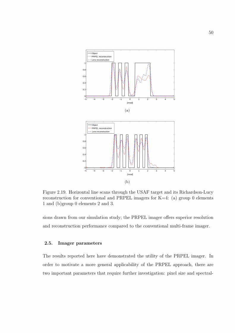
50
−5 −4 −3 −2 −1 0 1 2 3 4 5
0
0.2
0.4
0.6
0.8
1
[mrad]
Object
PRPEL reconstruction
Lens reconstruction
(a)
−5 −4 −3 −2 −1 0 1 2 3 4 5
0
0.2
0.4
0.6
0.8
1
[mrad]
Object
PRPEL reconstruction
Lens reconstruction
(b)
Figure 2.19. Horizontal line scans through the USAF target and its Richardson-Lucyreconstruction for conventional and PRPEL imagers for K=4: (a) group 0 elements1 and (b)group 0 elements 2 and 3.
sions drawn from our simulation study; the PRPEL imager offers superior resolution
and reconstruction performance compared to the conventional multi-frame imager.
2.5. Imager parameters
The results reported here have demonstrated the utility of the PRPEL imager. In
order to motivate a more general applicability of the PRPEL approach, there are
two important parameters that require further investigation: pixel size and spectral-

51
1 2 3 4 5 6 7 8
0.2
0.3
0.4
0.5
0.6
0.7
Number of frames − K
Ang
ular
res
olut
ion
[mra
d]
Lens ImagerPRPEL Imager
Diffraction−limited resolution
(a)
1 2 3 4 5 6 7 8
1
1.5
2
2.5
3
3.5
4
4.5
5
5.5
Number of frames − K
RM
SE
[% o
f dyn
amic
ran
ge]
Lens Imager PRPEL Imager
(b)
Figure 2.20. (a) Rayleigh resolution and (b) RMSE versus number of frames formulti-frame imagers that employ smaller pixels and lower measurement SNR.
bandwidth. We consider two case studies in which these imaging system parameters
are modified in order to study their impact on overall imager performance.
2.5.1. Pixel size
Here we consider the effect of smaller pixel size which is typical of CMOS detectors ar-
rays, now commonly employed in many imagers. Consider a sensor having a pixel size
of 3.2µm resulting in a less severe under-sampling as compared with the 7.5µm pixel
size assumed earlier. This detector has a 100% fill-factor and a smaller FWC of 28000
electrons(lower SNR). All other parameters of the imaging system remain unchanged.
The under-sampling factor for the new sensor is F = 7 and the photon-limited SNR
is now 22dB. We repeat the simulation study of the overall imaging system perfor-
mance for both the conventional imager and the PRPEL imager. Fig. 2.20(a) shows
the plot of the resolution versus the number of frames for both imaging systems. This
plot shows that for K = 2 the PRPEL imager achieves a resolution of 0.3mrad while
the conventional imager resolution is only 0.5mrad. Fig. 2.20(b) shows the RMSE
performance of the two imagers versus the number of frames. For K = 2 the PRPEL

52
−15 −10 −5 0 5 10 150
0.2
0.4
0.6
0.8
1
1.2
1.4
1.6
x 10−3
Spatial dimension [µm]
Am
plitu
de
PSF − 10nmPSF − 150nm
Figure 2.21. The optical PSF obtained using PRPEL with both narrowband (10 nm)and broadband (150 nm) illumination.
imager achieves a RMSE of 3.2% compared to 4.0% for the conventional imager, an
improvement of nearly 20%. From these results we conclude that the PRPEL imager
remains a useful option for imagers with CMOS sensors that have smaller pixels and
a lower SNR.
2.5.2. Broadband operation
Recall that all our simulation studies have assumed a 10 nm spectral bandwidth so
far. In this section, we will relax this constraint and allow the spectral bandwidth
to increase to 150 nm, roughly equal to the bandwidth of the green band of the
visible spectrum. All other imaging system parameters remain unchanged (using the
original 7.5µm sensor). There is a two-fold implication of the increased bandwidth.
First, because we accept a wider bandwidth, the photon count increases resulting
in an improved measurement SNR. Within the PRPEL imager however, this SNR
increase is accompanied by increased chromatic dispersion and a smoothing of the
PRPEL PSF. This smoothing results in a worsening of the condition number for
the PRPEL imager. To illustrate the dispersion effect, Fig. 2.21 shows a plot of
the extended PRPEL PSF for both the 10 nm and the 150 nm bandwidths. The
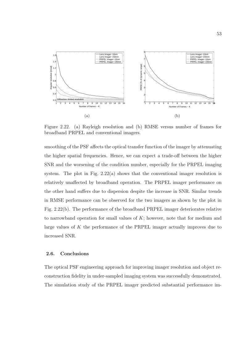
53
1 2 3 4 5 6 7 8 9 10 11 12 13 14 15 160.2
0.4
0.6
0.8
1
1.2
1.4
1.6
Number of frames − K
Ang
ular
res
olut
ion
[mra
d]
Lens Imager−10nmLens Imager−150nm PRPEL Imager−10nmPRPEL Imager−150nm
Diffraction−limited resolution
(a)
1 2 3 4 5 6 7 8 9 10 11 12 13 14 15 16161
2
3
4
5
6
7
8
Number of Frames − K
RM
SE
[% o
f dyn
amic
ran
ge]
Lens Imager−10nmLens Imager−150nmPRPEL Imager−10nmPRPEL Imager−150nm
(b)
Figure 2.22. (a) Rayleigh resolution and (b) RMSE versus number of frames forbroadband PRPEL and conventional imagers.
smoothing of the PSF affects the optical transfer function of the imager by attenuating
the higher spatial frequencies. Hence, we can expect a trade-off between the higher
SNR and the worsening of the condition number, especially for the PRPEL imaging
system. The plot in Fig. 2.22(a) shows that the conventional imager resolution is
relatively unaffected by broadband operation. The PRPEL imager performance on
the other hand suffers due to dispersion despite the increase in SNR. Similar trends
in RMSE performance can be observed for the two imagers as shown by the plot in
Fig. 2.22(b). The performance of the broadband PRPEL imager deteriorates relative
to narrowband operation for small values of K; however, note that for medium and
large values of K the performance of the PRPEL imager actually improves due to
increased SNR.
2.6. Conclusions
The optical PSF engineering approach for improving imager resolution and object re-
construction fidelity in under-sampled imaging system was successfully demonstrated.
The simulation study of the PRPEL imager predicted substantial performance im-

54
provements over a conventional multi-frame imager. The PRPEL imager was shown
to offer as much as 50% resolution improvement and 20% RMSE improvement as
compared to the conventional imager. The experimental results confirmed these pre-
dicted performance improvements. We also applied the non-linear Richardson-Lucy
reconstruction technique to the experimental data. The results obtained showed
that imager performance is substantially improved with non-linear techniques. In
this chapter, the application of optical PSF engineering method to the object re-
constructed task has shown the potential benefits of the joint-optimization design
approach. In next chapter, we extend the application of the optical PSF engineering
method to an iris-recognition task.
55
Chapter 3
Optical PSF Engineering: Iris Recognition Task
In this chapter we will apply the optical PSF engineering approach to the task of
iris-recognititon to overcome the performance degradations introduced by an under-
sampled imaging system. Note that the metric for quantifying the imaging system
performance for a particular task plays a critical role in the joint-optimization design
approach. For the object reconstruction task we had employed two metrics: 1) res-
olution and 2) RMSE. Here we will use the statistical metric of false rejection ratio
(FRR) (evaluated at a fixed false acceptance ratio (FAR)) for quantifying the imaging
system performance for the iris-recognition task.
3.1. Introduction
Many modern defense and security applications require automatic recognition and
verification services that employ a variety of biometrics such as facial features, hand
shape, voice, fingerprints, and iris. The iris is the annular region between the pupil
and the outer white sclera of the eye. Iris-based recognition has been gaining pop-
ularity in recent years and it has several advantages compared to other traditional
biometrics such as fingerprints and facial features. The iris-texture pattern represents
a high-density of information and the resulting statistical uniqueness can yield false
recognition rates as low as 1 in 1010 [41, 42, 43]. Further, it has been found that
the human iris is stable over the lifetime of an individual and is therefore considered
to be a reliable biometric [44]. Iris-based recognition systems rely on capturing the
iris-texture pattern with a high-resolution imaging system. This places stringent de-
mands on imaging optics and sensor design. In the case where the detector pixel size

56
limits the overall resolution of the imaging system, the under-sampling in the sensor
array can lead to degradation of the iris-recognition performance. Therefore, over-
coming the detector-induced under-sampling becomes a vital issue in the design of
an iris-recognition imaging system. One approach to improve the resolution beyond
the detector limit employs multiple sub-pixel shifted measurements within a TOMBO
imaging system architecture [19, 20]. However, this approach does not exploit the
optical degrees of freedom available to the designer and more importantly it does not
address the specific nature of the iris-recognition task. We note that there are some
studies that have exploited the optical degrees of freedom to extend the depth-of-field
of iris-recognition systems [45, 46], but we are not aware of any previous work that
has examined under-sampling in iris-recognition imaging systems. In this chapter,
we propose an approach that involves engineering the optical point spread function
(PSF) of the imaging system in conjunction with use of multiple sub-pixel shifted
measurements. It is important to note that the goal of our approach is to maxi-
mize the iris-recognition performance and not necessarily the overall resolution of the
imaging system. To accomplish this goal, we employ an optimization framework to
engineer the optical PSF and optimize the post-processing system parameters. The
task-specific performance metric used within our optimization framework is FRR for
a given FAR [47]. The mechanism of modifying the optical PSF employs a phase-
mask in the aperture-stop of the imaging system. The phase-mask is defined with
Zernike polynomials and the coefficient of these polynomials serve as the optical de-
sign parameters. The optimization framework is used to design imaging systems for
various numbers of sub-pixel shifted measurements. The CASIA iris database [48] is
used in the optimization framework and it also serves to quantify the performance of
the resulting optimized imaging system designs.

57
X−axis
Y−
axis
Z−axis
Object
Phase−mask
Imaging Optics
Detector−
array
Figure 3.1. PSF-engineered multi-aperture imaging system layout.
3.2. Imaging System Model
In this study, our iris-recognition imaging system is composed of three components: 1)
the optical imaging system, 2) the reconstruction algorithm, and 3) the recognition al-
gorithm. The optical imaging system consists of multiple sub-apertures with identical
optics. This multi-aperture imaging system produces a set of sub-pixel shifted im-
ages on the sensor array. The task of the reconstruction algorithm is to combine these
image measurements to form an estimate of the object. Finally, the iris-recognition
algorithm operates on this object estimate and either accepts or rejects the iris as a
match. We begin by describing the multi-aperture imaging system.
3.2.1. Multi-aperture imaging system
Fig. 3.1 shows the system layout of the multi-aperture(MA) imaging system. The
number of sub-imagers comprising the MA imaging system is denoted by K. The
sensor array in the focal plane of the MA imager generates K image measurements,
where the kth measurement (also referred to as a frame) is denoted by gk. The detector
pitch d of the sensor array relative to the Nyquist sampling interval δ, determined by
the optical cut-off spatial frequency, defines the under-sampling factor: F = dδ× d
δ.
Therefore, for an object of size N × N pixels the under-sampled kth sub-imager

58
measurement gk is of dimension M ×M , where M = ⌈ N√F⌉. Mathematically, the kth
frame can be expressed as
gk = Hkf + nk, (3.1)
where f is a N2 × 1 dimensional vector formed by a lexicographic arrangement of a
two-dimensional (N ×N) discretized representation of the object, Hk is the M2 ×N2
discrete-to-discrete imaging operator of the kth sub-imager and nk denotes the M2×1
dimensional measurement error vector. Here we model the measurement error nk as
zero-mean additive white Gaussian noise (AWGN) with variance σ2n. Note that the
imaging operator Hk is different for each sub-imager and is expressed as
Hk = DCSk, (3.2)
where Sk is the N2 × N2 shift operator that produces a two-dimensional sub-pixel
shift (∆Xk,∆Yk) in the kth sub-imager, C is N2 × N2 convolution operator that
represents the optical PSF and D is the M2 × N2 down-sampling operator which
includes the effect of spatial integration over the detector and the under-sampling
caused by the sensor array. Note that the convolution operator C does not vary with
k because the optics are assumed to be identical in all sub-imagers. By combining
the K measurements we can form a composite measurement g = g1 g2 · · ·gK that
can be expressed in terms of the object vector f as follows
g = Hcf + n, (3.3)
where Hc = H1 H2 · · ·HK is the composite imaging operator of size KM2 × N2
obtained by stacking the K imaging operators corresponding to each of the K sub-
imagers and n is the composite noise vector defined as n = n1 n2 · · ·nK.As mentioned earlier, the optical PSF is engineered by placing a phase-mask in the
aperture-stop of each sub-imager. The pupil-function tpupil(ρ, θ) of each sub-imager
is expressed as [29]
tpupil(ρ, θ) = tamp(ρ)exp(j2π(nr − 1)tphase(ρ, θ)
λ
), (3.4)

59
where ρ and θ are the polar coordinate variables in the pupil, nr is the refractive index
of the phase-mask, tamp(ρ) = circ( ρDap
) is the circular pupil-amplitude function(Dap
denotes the aperture diameter), tphase(ρ, θ) represents the pupil-phase function and λ
is the wavelength. A Zernike-polynomial of order P is used to define the pupil-phase
function as follows
tphase(ρ, θ) =P∑
i=1
ai · Zi(ρ, θ), (3.5)
where ai is the coefficient of the ith Zernike polynomial denoted by Zi(ρ, θ) [49]. In
this work, we will use Zernike polynomials up to order P = 24. The resulting optical
PSF h(ρ, θ) is expressed as [28]
h(ρ, θ) =Ac
(λfl)4
∣∣∣∣Tpupil
(− ρ
λfl, θ
)∣∣∣∣2
, (3.6)
Tpupil(ω) = F2 tpupil(ρ, θ) , (3.7)
where ω is the two-dimensional spatial frequency vector, Ac is a normalization con-
stant with units of area, fl is the back focal length, and F2 denotes the 2-dimensional
forward Fourier transform operator.
A discrete representation of the optical PSF hd(l,m), required for defining the C
operator is obtained as follows
hd(l,m) =
∫ d2
− d2
∫ d2
− d2
h(x− ld, y −md)dxdy (l,m) : l = −L · · ·L,m = −L · · ·L,
(3.8)
where (2L + 1)2 is the number of samples used to represent the optical PSF. Note
that a lexicographic ordering of the hd(l,m) yields one row of C and all other rows
are obtained by lexicographically ordering the appropriately shifted version of this
discrete optical PSF.
3.2.2. Reconstruction algorithm
The measurements from the K sub-imagers comprising the MA imaging system form
the input to the reconstruction algorithm. We employ a reconstruction algorithm

60
Figure 3.2. Iris examples from the training dataset.
based on the linear minimum mean square error (LMMSE) criterion. The LMMSE
method is essentially a generalized form of the Wiener filter and operates on the
measurement in the spatial domain without the assumption of shift-invariance. Given
the imaging model specified in Eq. (3.3) the LMMSE operator W can be written
as [31]
W = RffHTc
(HcRffHT
c + Rnn
)−1, (3.9)
where Rff is the object auto-correlation matrix and Rnn is the noise auto-correlation
matrix. Here we assume that noise is zero-mean AWGN with variance σn2 and there-
fore Rnn = σ2nI. Note that for an object of size N2 and measurement of size KM2, the
size of W matrix is N2 ×KM2. For even a modest object size of 280× 280, as is the
case here, computing the W matrix becomes computationally very expensive. There-
fore, we adopt an alternate approach that does not rely on directly computing matrix
inverses but instead uses a conjugate-gradient method to compute the LMMSE solu-
tion iteratively. Before we describe the iterative algorithm, we first need a method to
estimate the object auto-correlation matrix Rff . We use a training set of 40 subjects
with 4 iris samples for each subject, randomly selected from the CASIA iris database

61
yielding a total of 160 iris object samples. Fig. 3.2 shows example iris-objects in the
training dataset. The kth iris object yields the sample auto-correlation function rkff
which is used to estimate the actual auto-correlation function as follows
Rff =1
160
160∑
k=1
rkff. (3.10)
The corresponding power spectral density Sff can be written as [50]
Sff (ρ) = F2(Rff ). (3.11)
To obtain a smooth approximation of the power spectral density we use the following
parametric function [51]
Sff (ρ) =σ2
f
(1 + 2πµdρ2)3
2
. (3.12)
Note that because the iris is circular, we assume a radially symmetric power spectrum
Sff . A least square fit to Sff (ρ) yields σf = 43589 and µd = 1.5.
In general, a conjugate-gradient algorithm minimizes the following form of quadratic
objective function Q [28]
Q(f) =1
2f tAf − btf . (3.13)
For the LMMSE criterion, A = HTc Hc + σ2R−1
ffand b = HT
c g. Within our iterative
conjugate gradient-based algorithm we use a conjugate-vector pj instead of the gradi-
ent of the objective Q(f) to achieve a faster convergence to the LMMSE solution [52].
The k + 1th update rule can be expressed as [28]
fk+1 = fk + αkpk (3.14)
αk = −ptk∇Qk
dk, (3.15)
where ∇Qk denotes the gradient of objective function Qk evaluated at the kth step and
pk is conjugate to all previous pj , j < k (i.e. ptjApk = djδjk), δjk is the Kronecker-
delta function, and dk is the ‖ · ‖2 norm of pk. The stopping criterion is specified as
when the residual vector rk = ∇Qk = Afk − b changes less than β% over the last 4
iterations (i.e.rk−4−rk
rk−4≤ β
100).

62
(a) (b)
θ
ρ
50 100 150 200
102030
(c)
θ
ρ
50 100 150 200 250 300 350 400
102030
(d)
Figure 3.3. Examples of (a) iris-segmentation, (b) masked iris-texture region, (c)unwrapped iris, and (d) iris-code.
63
3.2.3. Iris-recognition algorithm
The object estimate obtained with the reconstruction algorithm is processed by the
iris-recognition algorithm to make the final decision. There are three main processing
steps that form the basis of the iris-recognition algorithm. The first step involves
a segmentation algorithm that extracts the iris, pupil, and the eye-lid regions from
the reconstructed object. The segmentation algorithm used in this work is adapted
from Ref. [53] with the addition of eye-lid boundary detection. The output of the
segmentation algorithm yields an estimate of the center and radius of the circular
pupil and iris regions and also the boundaries of the upper and lower eyelids in
the object. Fig. 3.3(a) shows an example iris image that was processed with the
segmentation algorithm. The pupil and iris regions are outlined by circular boundaries
and the upper/lower eyelid edges are represented by the elliptical boundaries. This
information is used to generate a mask M(x, y) that extracts the annular region
between iris and pupil boundaries which contains only the unobscured iris-texture
region. An example of the masked iris region is shown in Fig. 3.3(b). The extracted
iris-texture region is the input to the next processing step. Given the center and
radius of the pupil and the iris regions, the annular iris-texture region is unwrapped
into a rectangular area a(ρ, θ) using Daugman’s homogenous rubber sheet model [54].
The size of the rectangular region is specified as Lρ×Lθ with Lρ rows along the radial
direction and Lθ columns along the angular direction. Fig. 3.3(c) shows an example
of an unwrapped rectangular region with Lρ = 36 and Lθ = 224. In the next step,
a complex log-scale Gabor filter is applied to each row to extract the phase of the
underlying iris-texture pattern. The complex log-scale Gabor filter spectrum Glog(ρ)
is defined as [55]
Glog(ρ) = exp
(
−log( ρ
ρo)
2log(σg
ρo)
)
, (3.16)
where ρo is the center frequency of the filter and σg specifies its bandwidth. Note that
this filter is only applied along the angular direction which corresponds to pixels on

64
the circumference of a circle in the original object. The angular direction is chosen
over the radial direction because the maximum texture variation occurs along this
direction [53]. The phase of the complex output of each Gabor filter is then quantized
into four quadrants using two bits. The 4-level quantized phase is coded using a Grey
code so that the difference between two adjacent quadrants is one bit. The Grey
coding scheme also ensures that any misalignment between two similar iris-codes
results in a minimum of errors. The quantized phase results in a binary pattern,
shown in Fig. 3.3(d), which is referred to as an “iris-code.”
In the final step, the iris-recognition task is performed based on the iris-code
obtained from a test object. To determine whether the given iris-code denoted by
tcode, matches any iris-code in the database, a score is computed. The score denoted
by s(tcode) is defined as
s(tcode) = mink,i
dhd(tcodeckmask, Ri(r
kcode)c
kmask), (3.17)
where rkcode is the kth reference iris-code in the database, ckmask is a mask that represents
the unobscured bits common among both the test and the reference iris-codes, Ri is
a shift operator which performs an i-pixel shift along the angular direction, and dhd
is the Hamming distance operator. All shifts in the range i : −O · · · + O are
considered, where O denotes the maximum shift. The dhd operator is defined as
follows
dhd(tcodecmask, rcodecmask) =
∑(tcodecmask ⊕ rcodecmask)
W, (3.18)
where W is the weight (i.e. number of all 1s) of the mask cmask. The normalized
Hamming distance score defined in Eq. (3.18) is computed over all iris-codes in the
database. The iris-code is shifted to account for any rotation of the iris in the object.
Finally, the following decision rule is applied to the minimum iris score s(tcode)
s(tcode)H0
≶H1
THD, (3.19)
this translates to: accept the null hypothesis H0 if the score is less than threshold

65
0.05 0.10 0.15 0.20 0.25 0.30 0.35 0.40 0.45 0.50 0.550
0.05
0.10
0.15
0.20
0.25
0.30
0.35
0.40
Normalized Hamming Distance (HD)
Pro
babi
lity
dens
ity
Inter−class probability density
Intra−class probability density
T
FARFRR
THD
Figure 3.4. Illustration of FRR and FAR definitions in the context of intra-class andinter-class probability densities.
THD, otherwise accept the alternative hypothesis H1. The null-hypothesis H0 implies
that the test iris was correctly recognized and the alternate-hypothesis H1 indicates
that test iris was mis-classified. The threshold THD determines the performance of
the iris-recognition system as summarized by the FRR and FAR statistics.
3.3. Optimization framework
The goal of our optimization framework is to enable the design of an iris-recognition
system that minimizes FRR for a fixed FAR in the presence of under-sampling.
Fig. 3.4 illustrates the definitions of FRR and FAR in the context of intra-class
distance and inter-class distance probability densities. Intra-class distance refers to
the set of distances between iris-codes of the same subject, whereas the inter-class
distance refers to the set of distances between iris-codes from different subjects. The
rational behind this choice of performance metric is that the cost of not recognizing
an iris which is actually enrolled (false rejection error) in the database is significantly
higher than recognizing an iris as a match when it is not enrolled in the database
(false acceptance error). Note that the FRR and FAR errors can not be reduced

66
simultaneously. In this study we set FAR to 0.001. This value of FAR may not
represent an optimal choice for an actual system however, here it only serves as a
representative value in our optimization framework.
In the MA imaging system the coefficients of the Zernike polynomials, that de-
scribe the pupil-phase function, represent the optical design parameters. The param-
eters of the reconstruction algorithm (e.g. β) and iris-recognition algorithm (e.g. ρo,
σg, Lρ, Lθ, O) comprise the degrees of freedom available in the computational do-
main. Ideally, a joint-optimization of the optical and the post-processing parameters
of the imaging system would yield the maximum improvement in the iris-recognition
performance. However, the resulting optimization process would be computationally
intractable due to the high computational complexity of evaluating the objective func-
tion coupled with the large number of design variables. Here the objective function
computation involves the estimation of the intra-class and inter-class iris distance
probability densities. This in turn requires computing iris-codes from a set of re-
constructed iris-objects and comparing to the reference iris database. Here we use a
training dataset with 160 iris object samples as described in Subsection 3.2.2. In or-
der to obtain a reliable estimate of the inter-class and intra-class distance probability
densities, we need to generate a large set of iris-code samples. This is achieved by
simulating an iris object for 10 random noise realizations yielding as many iris-codes
for each iris-object. Thus, a single evaluation of the objective function effectively
results in simulation of 1600 iris objects through the imaging system. Therefore, op-
timizing over all available degrees of freedom becomes a computationally prohibitive
task.
In our optimization framework, we adopt an alternative approach that departs
from the ideal joint-optimization goal. We note that our approach still involves a
joint-optimization of optical and computational parameters while reducing the com-
putational complexity by splitting the optimization into two separate steps. Note
that the iris-recognition algorithm parameters are inherently a function of the iris-

67
texture statistics and are not strongly dependent on the optics. For example, the
center frequency and the bandwidth of the log Gabor filter are tuned to the spa-
tial frequency distribution of the iris-texture that contains the most discriminating
information. Further, the parameters Lρ and Lθ are dependent on the correlation
length of iris-texture along radial and angular directions respectively. This allows us
to optimize the iris-recognition algorithm parameters independent of the optics and
the reconstruction algorithm. Therefore, the first optimization step involves opti-
mizing the iris-recognition algorithm parameters to minimize the FRR. For this step
the detector pitch is chosen such that there is no under-sampling and no phase-mask
is used in the optics. The optimization is performed with a coarse-to-fine search
method using the iris objects from the training dataset. It is found that Lρ = 36,
Lθ = 224, ρo = 1/18, and σg = 0.4 yield the optimal performance. The number of left
and right shifts required to achieve optimal performance is O = 8 in each direction.
As a result of the first step, the second optimization step is reduced to the task of
optimizing the optical and reconstruction algorithm parameters which becomes com-
putationally tractable. The optical system parameters include the P coefficients of
the Zernike polynomials. The reconstruction algorithm parameter β, associated with
the stopping condition in the iterative conjuage-gradient algorithm, is the only post-
processing design variable used in this optimization step. Note that the values of the
iris-recognition algorithm parameters remain fixed during this optimization step.
Our optimization framework employs a simulated tunneling algorithm, a global
optimization technique [56], to perform the second optimization step. This global
optimization algorithm is implemented in a MPI-based environment [57] that allows
it to run on multiple processors in parallel, thereby decreasing the computation time
required for each iteration. The simulated tunneling algorithm is run for 4000 itera-
tions to ensure that convergence is achieved. This optimization framework is used to
design imaging systems with an under-sampling of F = 8×8 that use K = 1, K = 4,
K = 9, and K = 16 frames. The sub-pixel shifts for K frames is chosen as multiples

68
Under-sampling Frames Conventional ZPEL
F = 1 × 1 0.133F = 8 × 8 K = 1 0.458 0.295F = 8 × 8 K = 4 0.153 0.128F = 8 × 8 K = 9 0.140 0.117F = 8 × 8 K = 16 0.135 0.113
Table 3.1. Imaging system performance for K = 1, K = 4, K = 9, and K = 16 ontraining set.
of ∆ = d√K
along each direction, where d is the detector pitch/size. For example,
for K = 4 the sub-pixel shifts are (∆X ,∆Y ) : (0, 0), (d2, 0), (0, d
2), (d
2, d
2). The noise
variance σ2n is set so that the measurement signal to noise ratio (SNR) is equal to
60 dB. From here onwards the optimized imaging system will be referred to as the
Zernike phase-enhanced lens (ZPEL) imaging system. In the next section, we discuss
the performance of the optimized ZPEL imager and compare it to a conventional
imaging system.
3.4. Results and Discussion
The under-sampling in the sensor array degrades the performance of the iris-recognition
imaging system. With an under-sampling factor of F = 8 × 8 we find that FRR =
0.458 as compared to FRR = 0.133 without under-sampling in the conventional imag-
ing system. This represents a significant reduction in performance and highlights the
need to mitigate the effect of under-sampling. Increasing the number of sub-pixel
shifted frames from K = 1 to K = 16 improves the performance of the conventional
imaging system, as evident from the FRR data shown in Table (3.1). To ensure a
fair comparison among imaging systems with various number of frames, we enforce
a total photon constraint. This constraint implies that the total number of photons
available to each imager (i.e. summed over all frames) is fixed. Therefore, for an
imaging system using K frames the measurement noise variance must be scaled by

69
a factor of K. For example, the measurement noise variance in an imaging system
with K = 4 frames is set to σ2K = 4σ2
n, where σ2n is the measurement noise variance of
the imaging system with K = 1. Subject to this constraint, we expect that a ZPEL
imaging system designed within the proposed optimization framework would improve
upon the performance of the conventional imaging system.
We begin by examining the result of optimizing the ZPEL imaging system with
K = 1. Fig. 3.5(a) shows the Zernike phase-mask and Fig. 3.5(b) shows the cor-
responding optical PSF of the optimized ZPEL imager. For comparison purpose,
Fig. 3.5(c) shows the optical PSF of the conventional imager. The phase-mask spans
over the extent the aperture-stop, where 0.5 corresponds to the radius (Dap
2) of the
aperture. The optical PSF is plotted over the normalized scale of [−1, 1] where 1 cor-
responds to the detector size d. Note that the large spatial extent of the PSF relative
to that of a conventional imaging system suggests that high spatial frequencies in the
corresponding modulation transfer function (MTF) would be suppressed. Fig. 3.6
shows plots of various cross-sections of the two-dimensional MTF. Here spatial fre-
quency is plotted on the normalized scale of [−1, 1], where 1 corresponds to the optical
cut-off frequency ρc. Observe that the MTF reduces rapidly with increasing spatial
frequency. This is a result of the optimization process suppressing the MTF at the
high spatial frequencies to reduce the effect of aliasing. Furthermore, the non-zero
MTF at mid-spatial frequencies allows the reconstruction algorithm to potentially
recover some information in this region which is crucial for the iris-recognition task.
The expected performance improvement is clearly evident from a lower FRR = 0.295
achieved by the optimized ZPEL imaging system as opposed to FRR = 0.458 of the
conventional imaging system. This is equivalent to an improvement of 32.7% which is
significant, given the ZPEL imager would result in nearly 163 fewer false rejections on
average for every 1000 iris tested. Similarly, with K = 4 the optimized ZPEL imager
yields an FRR = 0.153 that is 16.3% lower than FRR = 0.128 of the conventional
imaging system. Fig. 3.7(a) and Fig. 3.7(b) show the phase-mask and the optical PSF

70
−0.5 −0.4 −0.3 −0.2 −0.1 0 0.1 0.2 0.3 0.4 0.5
−0.5
−0.4
−0.3
−0.2
−0.1
0
0.1
0.2
0.3
0.4
0.5 −10
−5
0
5
10
15
20
25
(a)
−1 −0.8 −0.6 −0.4 −0.2 0 0.2 0.4 0.6 0.8 1
−1
−0.8
−0.6
−0.4
−0.2
0
0.2
0.4
0.6
0.8
1
(b)
−1 −0.8 −0.6 −0.4 −0.2 0 0.2 0.4 0.6 0.8 1
−1
−0.8
−0.6
−0.4
−0.2
0
0.2
0.4
0.6
0.8
1
(c)
Figure 3.5. Optimized ZPEL imager with K = 1 (a) pupil-phase, (b) optical PSF,and (c) optical PSF of conventional imager .

71
−1 −0.9 −0.8 −0.7 −0.6 −0.5 −0.4 −0.3 −0.2 −0.1 0 0.1 0.2 0.3 0.4 0.5 0.6 0.7 0.8 0.9 10
0.1
0.2
0.3
0.4
0.5
0.6
0.7
0.8
0.9
1
Spatial frequency
Mod
ulat
ion
X−direction
Y−direction
θ=135o direction
θ=45o direction
Conventional
Figure 3.6. Cross-section MTF profiles of optimized ZPEL imager with K = 1.
−0.5 −0.4 −0.3 −0.2 −0.1 0 0.1 0.2 0.3 0.4 0.5
−0.5
−0.4
−0.3
−0.2
−0.1
0
0.1
0.2
0.3
0.4
0.5−10
−8
−6
−4
−2
0
2
4
6
8
10
(a)
−1 −0.8 −0.6 −0.4 −0.2 0 0.2 0.4 0.6 0.8 1
−1
−0.8
−0.6
−0.4
−0.2
0
0.2
0.4
0.6
0.8
1
(b)
Figure 3.7. Optimized ZPEL imager with K = 4: (a) pupil-phase and (b) opticalPSF.

72
−1 −0.9 −0.8 −0.7 −0.6 −0.5 −0.4 −0.3 −0.2 −0.1 0 0.1 0.2 0.3 0.4 0.5 0.6 0.7 0.8 0.9 10
0.1
0.2
0.3
0.4
0.5
0.6
0.7
0.8
0.9
1.0
Spatial frequency
Mod
ulat
ion
X−direction
Y−direction
θ=45o direction
θ=135o direction
Conventional
Figure 3.8. Cross-section MTF profiles of optimized ZPEL imager with K = 4.
of this optimized ZPEL imager respectively. Note that the optical PSF has a smaller
extent compared to that forK = 1. The use of 4 frames as opposed to 1 frame reduces
the effective under-sampling by a factor of 2 in each direction. Thus, we expect as
a result of the optimization, the MTF in this case would be higher, especially in the
mid-spatial frequencies compared to the MTF of the ZPEL imager with K = 1. This
is confirmed by the plot of the MTF in Fig. 3.8. The MTF at mid-spatial frequencies
is significantly higher in Fig. 3.8 compared to that in Fig. 3.6. It is also interesting
to note that the FRR = 0.128 achieved by this optimized ZPEL imager is actually
lower than FRR = 0.133 of the conventional imaging system without under-sampling.
This clearly highlights the effectiveness of the optimization framework; by not only
overcoming the performance degradation due under-sampling but also successfully
incorporating the task-specific nature of the iris-recognition task in the ZPEL imager
design to enhance the performance beyond that of the conventional imager.
Fig. 3.9(a) and Fig. 3.9(b) show the Zernike phase-mask and the optical PSF of
the optimized ZPEL imager with K = 9. The ZPEL imager achieves a FRR = 0.117
compared to FRR = 0.140 for the conventional imaging system, an improvement of
16.4%. The MTF of this imaging system is shown in Fig. 3.10. The optimized ZPEL

73
−0.5 −0.4 −0.3 −0.2 −0.1 0 0.1 0.2 0.3 0.4 0.5
−0.5
−0.4
−0.3
−0.2
−0.1
0
0.1
0.2
0.3
0.4
0.5
−3
−2
−1
0
1
2
(a)
−1 −0.8 −0.6 −0.4 −0.2 0 0.2 0.4 0.6 0.8 1
−1
−0.8
−0.6
−0.4
−0.2
0
0.2
0.4
0.6
0.8
1
(b)
Figure 3.9. Optimized ZPEL imager with K = 9: (a) pupil-phase and (b) opticalPSF.
−1 −0.9 −0.8 −0.7 −0.6 −0.5 −0.4 −0.3 −0.2 −0.1 0 0.1 0.2 0.3 0.4 0.5 0.6 0.7 0.8 0.9 10
0.1
0.2
0.3
0.4
0.5
0.6
0.7
0.8
0.9
1.0
Spatial frequency
Mod
ulat
ion
X−direction
Y−direction
θ=45o direction
θ=135o direction
Conventional
Figure 3.10. Cross-section MTF profiles of optimized ZPEL imager with K = 9.

74
−0.5 −0.4 −0.3 −0.2 −0.1 0 0.1 0.2 0.3 0.4 0.5
−0.5
−0.4
−0.3
−0.2
−0.1
0
0.1
0.2
0.3
0.4
0.5 −4
−3
−2
−1
0
1
2
3
4
(a)
−1 −0.8 −0.6 −0.4 −0.2 0 0.2 0.4 0.6 0.8 1
−1
−0.8
−0.6
−0.4
−0.2
0
0.2
0.4
0.6
0.8
1
(b)
Figure 3.11. Optimized ZPEL imager with K = 16: (a) pupil-phase and (b) opticalPSF.
−1 −0.9 −0.8 −0.7 −0.6 −0.5 −0.4 −0.3 −0.2 −0.1 0 0.1 0.2 0.3 0.4 0.5 0.6 0.7 0.8 0.9 10
0.1
0.2
0.3
0.4
0.5
0.6
0.7
0.8
0.9
1.0
Spatial frequency
Mod
ulat
ion
X−direction
Y−direction
θ=45o direction
θ=135o direction
Conventional
Figure 3.12. Cross-section MTF profiles of optimized ZPEL imager with K = 16.
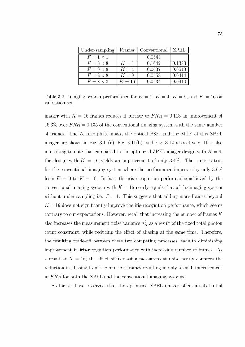
75
Under-sampling Frames Conventional ZPEL
F = 1 × 1 0.0543F = 8 × 8 K = 1 0.1642 0.1383F = 8 × 8 K = 4 0.0637 0.0513F = 8 × 8 K = 9 0.0558 0.0444F = 8 × 8 K = 16 0.0534 0.0440
Table 3.2. Imaging system performance for K = 1, K = 4, K = 9, and K = 16 onvalidation set.
imager with K = 16 frames reduces it further to FRR = 0.113 an improvement of
16.3% over FRR = 0.135 of the conventional imaging system with the same number
of frames. The Zernike phase mask, the optical PSF, and the MTF of this ZPEL
imager are shown in Fig. 3.11(a), Fig. 3.11(b), and Fig. 3.12 respectively. It is also
interesting to note that compared to the optimized ZPEL imager design with K = 9,
the design with K = 16 yields an improvement of only 3.4%. The same is true
for the conventional imaging system where the performance improves by only 3.6%
from K = 9 to K = 16. In fact, the iris-recognition performance achieved by the
conventional imaging system with K = 16 nearly equals that of the imaging system
without under-sampling i.e. F = 1. This suggests that adding more frames beyond
K = 16 does not significantly improve the iris-recognition performance, which seems
contrary to our expectations. However, recall that increasing the number of frames K
also increases the measurement noise variance σ2K as a result of the fixed total photon
count constraint, while reducing the effect of aliasing at the same time. Therefore,
the resulting trade-off between these two competing processes leads to diminishing
improvement in iris-recognition performance with increasing number of frames. As
a result at K = 16, the effect of increasing measurement noise nearly counters the
reduction in aliasing from the multiple frames resulting in only a small improvement
in FRR for both the ZPEL and the conventional imaging systems.
So far we have observed that the optimized ZPEL imager offers a substantial

76
Figure 3.13. Iris examples from the validation dataset.
improvement in the iris-recognition performance over the conventional imaging system
with an under-sampling detector array. However, these results were obtained using
the training dataset, the same data set that was used in the optimization process.
In order to estimate the actual performance of the optimized ZPEL imaging system
independent of the training dataset we need to assess it on a validation dataset. The
validation dataset consists of 44 distinct iris subjects with 7 samples of each iris,
selected from the CASIA database, resulting in a total of 308 iris samples. Fig. 3.13
shows example iris-objects from the validation dataset. Note that none of the iris
samples in the validation dataset appear in the training dataset. We use a total of 30
noise realizations for each iris-object to estimate the FRR from the intra-class and
inter-class densities. The FRR data for the validation dataset is shown in Table (3.2).
The optimized ZPEL imager for K = 1 yields a FRR = 0.138 on the validation
dataset as compared to FRR = 0.164 for the conventional imaging system. This
represents a performance improvement of about 15.9% over the conventional imaging
system, which is nearly half of the 32.7% improvement that was obtained on the
training dataset. This difference in performance can be explained by considering the
fact that the optimization process does not distinguish between the effect of under-
sampling and the statistics of the particular iris samples comprising the training

77
dataset. As a result, the imaging system is optimized jointly towards mitigating
the effect of under-sampling and adapting to the statistics of the iris samples in the
training dataset. We cannot expect the performance of the ZPEL imaging system to
be the same on the validation and training dataset, because the statistics of the iris
samples are different in the two datasets. However, it is important to add that the
difference between the performance on training and validation dataset will reduce as
the size of the training dataset is increased and it becomes more representative of the
true iris statistics.
In the case of K = 4, the ZPEL imager achieves an FRR = 0.0513 which is
an improvement of 19.4% over FRR = 0.0637 of the conventional imaging system.
With K = 9 the optimized ZPEL imager yields a FRR = 0.0444 compared to
FRR = 0.0558 of the conventional imaging system. This represents an improvement
of 21.6%. For K = 16 frames, the optimized ZPEL imager results in FRR = 0.0534
an 21.0% reduction from FRR = 0.0440 of the conventional imaging system with the
same number of frames. Note that the FRR of both the optimized ZPEL imager and
the conventional imaging system do not reduce significantly from K = 9 frames to
K = 16 frames. This is due to the same underlying trade-off between measurement
information and measurement noise with increasing number of frames which was
observed in the case of the training dataset.
3.5. Conclusions
We have studied the degradation in the iris-recognition performance resulting from
an under-sampling factor of F = 8 × 8 and found that in a conventional imager, it
yields FRR = 0.458 compared to FRR = 0.133 when there is no under-sampling. We
describe a joint-optimization framework that exploits the optical and post-processing
degrees of freedom jointly to maximize the iris-recognition performance in the pres-
ence of under-sampling. The resulting ZPEL imager design uses an engineered optical

78
PSF together with multiple sub-pixel shifted measurements to achieve the perfor-
mance improvement. The ZPEL imager is designed for K = 1, K = 4, K = 9, and
K = 16 number of frames. On the training dataset, the optimized ZPEL imager
achieved performance improvement of nearly 33% for K = 1 compared to the con-
ventional imaging system. With K = 4 frames the ZPEL imager design achieved a
FRR which is nearly equal to that of a conventional imager without under-sampling.
The effectiveness of the optimization framework was highlighted by the ZPEL imager
design with K = 16 that achieved a FRR = 0.113, that is actually 15% better than
FRR = 0.133 of the conventional imager without under-sampling. The comparison
of the ZPEL imager and conventional imaging system performance using a validation
dataset provided further support for the performance improvements obtained on the
training dataset. On the validation dataset, the ZPEL imager design required only
K = 4 frames as opposed to K = 16 frames needed by the conventional imaging
system to equal the performance without under-sampling. Similarly, with K = 16
frames the optimized ZPEL imager obtained a 21.0% performance improvement over
the conventional imaging system without under-sampling. These results demonstrate
the utility of the optimization framework for designing task-specific ZPEL imagers
that overcome the performance degradation due to under-sampling. The performance
improvements achieved with the ZPEL imager designs provide further validation for
the optical PSF engineering method within the joint-optimization design framework.
The reconstruction and the recognition tasks highlight the the task-specific nature of
the joint-optimization design framework and emphasize the crucial role of task-specific
metrics in the imaging system design process.

79
Chapter 4
Task-Specific Information
In this chapter, we introduce the notion of task-specific information (TSI) as a mea-
sure of the information content of an image measurement relevant to a specific task.
TSI is an information-theoretic metric that provides an upper bound on the task-
specific performance of an imaging system independent of the post-processing algo-
rithm. In this chapter we derive the TSI metric and demonstrate its application to
imaging system analysis for various detection and classification tasks. We also use
the TSI as a design metric to extend the depth of field of an imager by engineering
its optical PSF.
4.1. Introduction
The information content of an image plays an important role in a wide array of
applications ranging from video compression to imaging system design [27, 58, 59, 60,
61, 62]. However, the computation of image information content remains a challenging
problem. The problem is made difficult by (a) the high dimensionality of useful
images, (b) the complex/unknown correlation structure among image pixels, and (c)
the lack of relevant probabilistic models. It is possible to estimate the information
content of an image by using some simplifying assumptions. For example, Gaussian
and Markovian models have both been used to estimate image information [60, 61, 63].
Transform domain techniques have also been studied (e.g., wavelet prior models) [64,
65].
As natural images possess a high degree of redundancy, it is generally understood
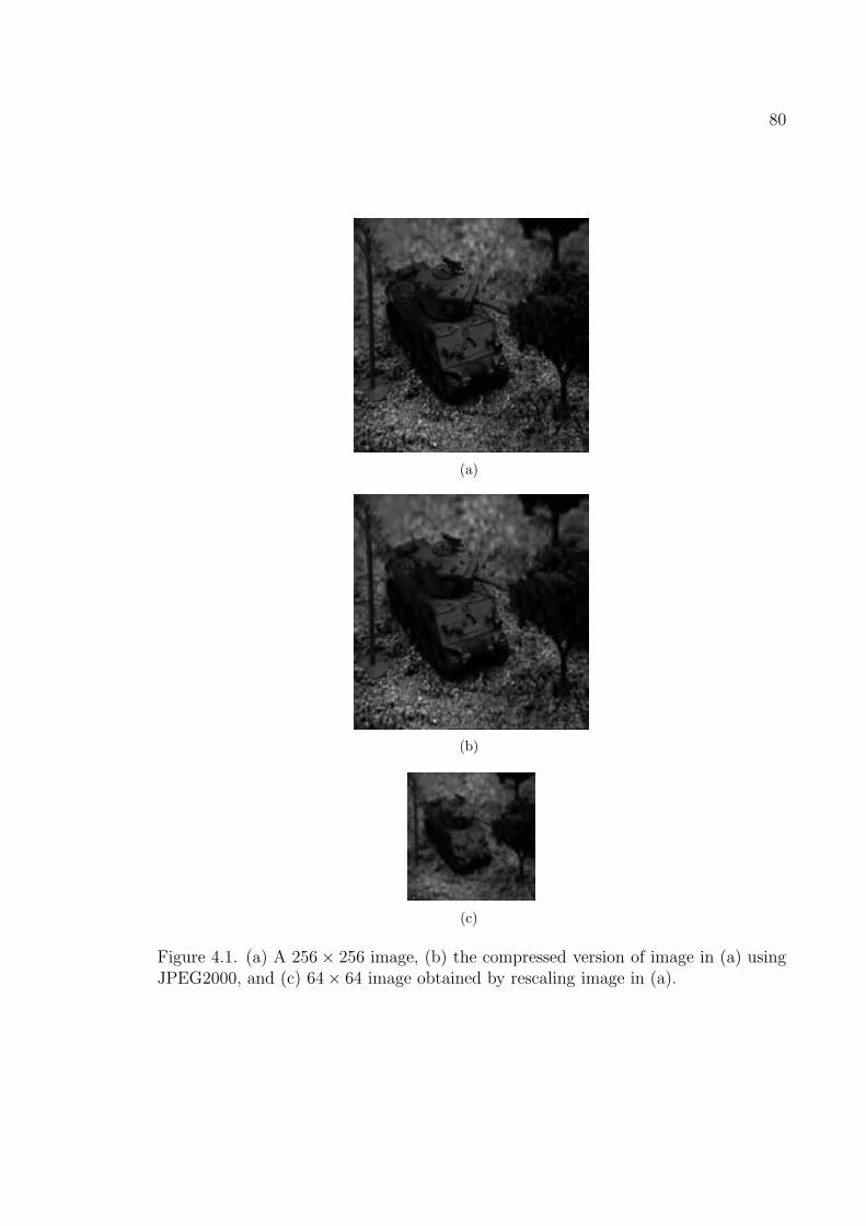
80
(a)
(b)
(c)
Figure 4.1. (a) A 256 × 256 image, (b) the compressed version of image in (a) usingJPEG2000, and (c) 64 × 64 image obtained by rescaling image in (a).

81
that the information content of a natural image is not simply the product of the
number of pixels and the number of bits per pixel. An upper bound on the information
content of an image can be obtained from the file size that is generated by a lossless
compression algorithm. Consider the 256× 256 pixel image shown in Fig. 4.1(a). An
uncompressed version of this image requires 8 bits per pixel resulting in a file size
of 524,288 bits; whereas, a lossless compression algorithm yields a file size of only
299,600 bits. A tighter upper bound might be obtained from a lossy compression
algorithm that yields a visually indistinguishable reconstruction. Fig. 4.1(b) depicts
a reconstruction obtained using JPEG2000 [66] which yields a compressed file size of
36,720 bits. We may conclude from the high quality of this reconstruction that bits
discarded from Fig. 4.1(a) to obtain Fig. 4.1(b) were not important to visual quality.
Imagery is often used in support of a computational task (e.g., automated target
recognition). For this reason we would like to pursue a simple extension to the result
shown in Fig. 4.1(b) in which the task performance, instead of visual quality, is the
relevant metric. In such a scenario we might expect there to be aspects of the imagery
that are important to the task and other aspects that are not. For example, if our
task is target detection, then the image shown in Fig. 4.1(c) may contain nearly
as much information as do the images in Fig. 4.1(a) and Fig. 4.1(b). The file size
required for the image in Fig. 4.1(c) is only 25,120 bits. Taking this process one step
further, a compression algorithm that actually performs target (a tank in this case)
detection would yield a compressed file size of only 1 bit to indicate either “target
present” or “target absent.” The preceding discussion demonstrates that an image
used for target detection will contain no more than 1 bit of relevant information.
We will refer to this relevant information as task-specific information (TSI) and the
remainder of this chapter represents an effort to describe/quantify TSI as an analysis
tool for several tasks and imaging systems of interest. What we describe here is a
formal approach to the computation of TSI. Such a formalism is important primarily
because it enables imager design and/or adaptation that strives to maximize the TSI

82
content of measurements. This has two implications: (a) imager resources can be
optimally allocated so that irrelevant information is not measured and thus task-
specific performance is maximized and/or (b) imager resources can be minimized
subject to a TSI constraint thus reducing imager complexity, cost, size, weight, etc.
It is worth mentioning that as TSI is a Shannon information-theoretic measure it can
be used to bound conventional task performance metrics such as probability of error
via Fano’s inequality for a classification task [67].
Although a formal approach for quantifying the Shannon information in a task-
specific way has not been previously reported, we do note important previous work
concerning the use of task-based metrics for image quality assessment by Barrett et
al. [8, 9, 10, 28]. This previous work has primarily focused on ideal observer models
and their application to various detection and estimation tasks.
The remainder of this chapter is organized as follows. Section 4.2 introduces a
formal framework for the definition of TSI and a method for its computation using
conditional mean estimators. We consider three example tasks: target detection,
target classification, and joint detection/classification and localization. In Section 4.3
we apply the TSI framework to two simple imaging systems; an ideal geometric imager
and a diffraction-limited imager for each of the three tasks. Section 4.4 extends
the imaging model to compressive imagers. The TSI framework is applied to the
analysis of two compressive imagers: a principal component compressive imager and
a matched-filter compressive imager. In Section 4.5 the TSI metric is used to extend
the depth of field of an imager for a texture classification task by engineering its optical
PSF. Section 4.6 summarizes the TSI framework and draws the final conclusions.
4.2. Task-Specific Information
We begin by considering the various components of an imaging system. A block
diagram depicting these components is shown in Fig. 4.2. In this model, the scene
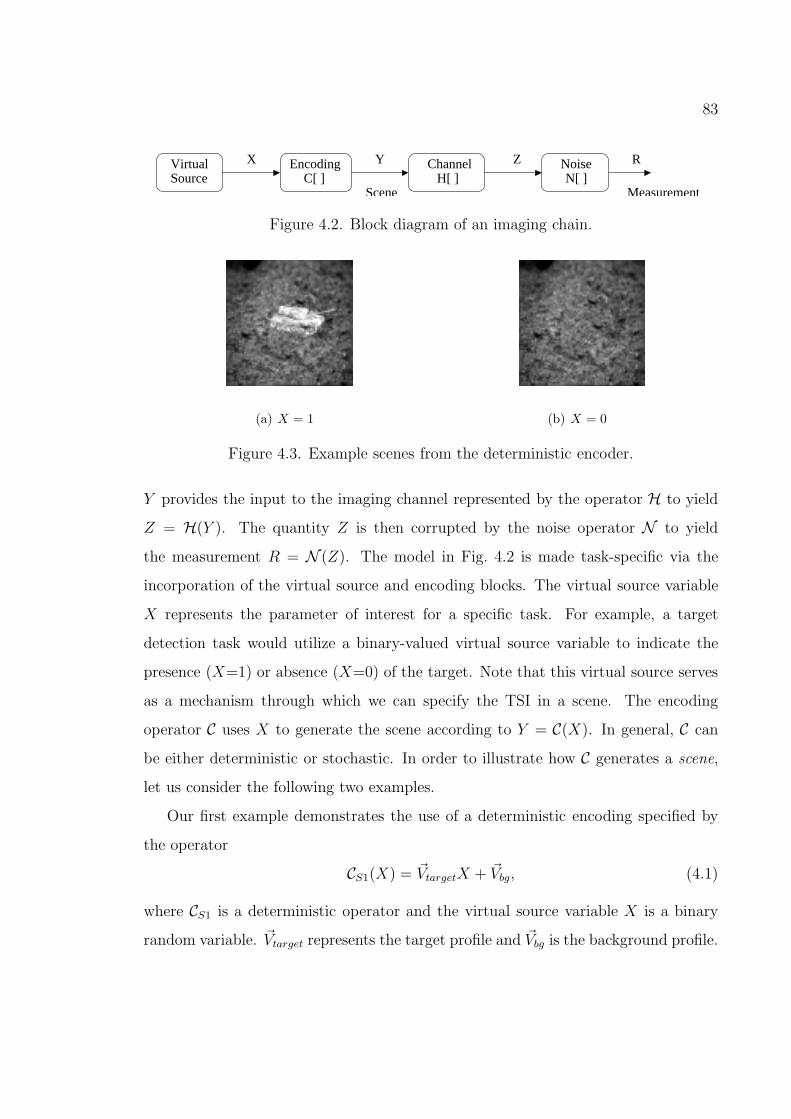
83
X Y Z R
SourceChannel
SceneH[ ]
NoiseN[ ]
Measurement
EncodingC[ ]
Virtual
Figure 4.2. Block diagram of an imaging chain.
(a) X = 1 (b) X = 0
Figure 4.3. Example scenes from the deterministic encoder.
Y provides the input to the imaging channel represented by the operator H to yield
Z = H(Y ). The quantity Z is then corrupted by the noise operator N to yield
the measurement R = N (Z). The model in Fig. 4.2 is made task-specific via the
incorporation of the virtual source and encoding blocks. The virtual source variable
X represents the parameter of interest for a specific task. For example, a target
detection task would utilize a binary-valued virtual source variable to indicate the
presence (X=1) or absence (X=0) of the target. Note that this virtual source serves
as a mechanism through which we can specify the TSI in a scene. The encoding
operator C uses X to generate the scene according to Y = C(X). In general, C can
be either deterministic or stochastic. In order to illustrate how C generates a scene,
let us consider the following two examples.
Our first example demonstrates the use of a deterministic encoding specified by
the operator
CS1(X) = ~VtargetX + ~Vbg, (4.1)
where CS1 is a deterministic operator and the virtual source variable X is a binary
random variable. ~Vtarget represents the target profile and ~Vbg is the background profile.

84
(a) X = 1
(b) X = 0
Figure 4.4. Example scenes from the stochastic encoder.
Note that ~Vtarget and ~Vbg are vectors formed by un-rastering a two-dimensional image
into a column vector. Fig. 4.3(a) and Fig. 4.3(b) show the encoder output for X = 1
and X = 0 respectively. The scene model defined by CS1 could be useful in a problem
where the task is to detect the presence or absence of a known target at a known
position in a known background.
Our second example demonstrates the use of a stochastic encoding specified by
the operator
CS2(X) = ~VtargetX + ~Vbg + ~Vtreeβ1 + ~Vshrubβ2, (4.2)
where X, ~Vtarget, and ~Vbg are the same as in Eq. (4.1). Clutter components ~Vtree
and ~Vshrub represent tree and shrub profiles respectively and are weighted by random
variables β1 and β2. Note that CS2 will depend on random variables β1 and β2;
therefore, CS2 is a stochastic operator. Fig. 4.4(a) and Fig. 4.4(b) show examples of
scene realizations generated by this stochastic encoding operator.
As X is the only parameter of interest for a given task, it is important to note
that the entropy of X defines the maximum task-specific information content of any
image measurement. Other blocks in the imaging chain may add entropy to the

85
image measurement R; however, only the entropy of the virtual source X is relevant
to the task. We may therefore define TSI as the Shannon mutual-information I(X;R)
between the virtual source X and the image measurement R as follows [67]
TSI ≡ I(X;R) = J(X) − J(X|R), (4.3)
where J(X) = −Elog(pr(X)) denotes the entropy of virtual source X, J(X|R) =
−Elog(pr(X|R) denotes the entropy of X conditioned on the measurement R, E·denotes statistical expectation, pr(·) denotes the probability density function, and
all the logarithms are taken to be base 2. Note that from this definition of TSI
we have I(X;R) ≤ J(X) indicating that an image cannot contain more TSI than
there is entropy in the variable representing the task. However, for most realistic
imaging problems computing TSI from Eq. (4.3) directly is intractable owing to the
dimensionality and non-Gaussianity of R. Numerical approaches may also prove
to be computationally prohibitive, even when using methods such as importance-
sampling, Markov Chain Monte Carlo(MCMC) or Bahl Cocke Jelinek Raviv(BCJR)
[68, 69, 70, 71, 72].
Recently, Guo et al. [73] demonstrated a direct relationship between the minimum
mean square error (mmse) in estimating X from R, and the mutual-information
I(X;R) for an additive Gaussian channel. Although the relation between estimation
mmse and Fisher information has been known via VanTree’s inequality [74], Guo’s
result connects estimation mmse with the Shannon information for the first time.
The result expresses mmse as a derivative of the mutual-information I(X;R) with
respect to signal to noise ratio. For a simple additive Gaussian noise channel we have
R =√sX +N, (4.4)
where N is the additive Gaussian noise with variance σ2 = 1 and s is the signal to
noise ratio. For this simple case we find that [73]
d
dsI(X;R) =
1
2mmse =
1
2E[|X − E(X|R)|2], (4.5)

86
where E(X|R) is the conditional mean estimator. This relation allows us to compute
mutual-information indirectly from mmse for an additive Gaussian channel without
any restrictions on the distribution of the virtual source variable X. It is interesting
to note that even though the source variable X is discrete valued, the conditional
mean estimator is a continuous variable which does not necessarily take values in the
range of the source variable X. For example, when X is a binary variable(0/1) the
conditional mean estimator will yield a real number between 0 and 1.
This result has been extended to the linear vector Gaussian channel for which
H[ ~X] = H ~X, where H denotes the matrix channel operator and ~X is the vector
channel input. The output of such a channel can be written as
~R =√sH ~X + ~N, (4.6)
where ~N follows a multivariate Gaussian distribution with covariance Σ ~N . In this
case, the Guo’s result becomes [75]
d
dsI( ~X; ~R) =
1
2E[||H ~X − E[H ~X|~R]||2]. (4.7)
The right hand side of Eq. (4.7) is the mmse in estimating H ~X rather than ~X and
therefore, we denote it by mmseH throughout the rest of this work to avoid confusion.
For an arbitrary noise covariance Σ ~N , mmseH can be computed using Tr(H†Σ−1~N
HE)
where E = E[( ~X − E[ ~X|~R])( ~X − E[ ~X |~R])T ], H† denotes the hermitian conjugate of
H and Tr(·) denotes the trace of the matrix. Therefore, the relationship between
mutual information and mmseH can be written as
d
dsI( ~X; ~R) =
1
2mmseH =
1
2Tr(H†Σ−1
~NHE). (4.8)
These results have also been extended to the case for which the channel input is
a random function of ~X, denoted by ~Y = C( ~X). The relation between I( ~X; ~R) and
mmseH for a random function C( ~X) is slightly different from the previous expression
in Eq. (4.8). Using the stochastic encoding model we have
~R =√sHC( ~X) + ~N. (4.9)

87
In this case the relation between mutual information and mmse can be expressed
as [75]
d
dsI( ~X; ~R) =
1
2mmseH , (4.10)
where mmseH = Tr(H†Σ−1~N
H(E~Y − E~Y | ~X)),
E~Y = E[(~Y − E(~Y |~R))(~Y − E(~Y |~R))T ],
E~Y | ~X = E[(~Y − E(~Y |~R, ~X))(~Y − E(~Y |~R, ~X))T ].
Next, we consider the application of these results to an important class of imaging
problems. We make the following assumptions about the general imaging chain model:
(1) The channel operator H is linear (discrete-to-discrete) and deterministic, (2) the
encoding operator C is linear and stochastic, and (3) the noise model N is additive
and Gaussian. We begin by developing some basic scene models for the tasks of
detection and classification.
4.2.1. Detection with deterministic encoding
For pedagogical purposes we begin with a scalar channel and a deterministic encoding.
Consider a simple task of detecting the presence or absence of a known scalar signal
t in the presence of noise. The measurement R is given as
R =√s t ·X +N (4.11)
where X is the virtual source variable that determines the signal present or absent
condition and N represents additive white Gaussian noise with variance σ2 = 1. Note
that here the encoding operator is deterministic and is defined as Cs(X) = t ·X. For
simplicity, we set HY = Y . Because X is a binary random variable with probability
distribution: Pr(X = 1) = p and Pr(X = 0) = 1 − p, we can assert
I(X;R) ≤ J(X) ≤ 1 bit, (4.12)

88
0 5 10 15 20 25 30 35 40 45 500
0.05
0.10
0.15
0.20
0.25
s
mm
se
(a)
0 5 10 15 20 25 30 35 40 45 500
0.2
0.4
0.6
0.8
1
s
Tas
k S
peci
fic In
form
atio
n [b
its]
mmse methoddirect method
(b)
Figure 4.5. (a) mmse and (b) TSI versus signal to noise ratio for the scalar detectiontask.
where the entropy of X is J(X) = −p log(p) − (1 − p) log(1 − p). Note that for
this simple detection task the received signal R contains at most 1 bit of task-specific
information. Therefore, the performance of any detection algorithm that operates on
the measurement R is upper bounded by the task-specific information.
We compute the mutual-information I(X;R) using two methods. The direct
method is based on the definition of mutual-information given in Eq. (4.3) wherein
differential entropies will be used owing to the continuous-valued nature of R. The
conditional differential entropy J(R|X) equals J(N) = 12ln(2πeσ2). Note that J(R)
is not straightforward to compute as R follows a mixture of Gaussian distribution
defined as
pr(R) =1√
2πσ2
(p exp
[−(R −√
st)2
2σ2
]+ (1 − p) exp
[− R2
2σ2
]). (4.13)
We therefore resort to numerical integration to compute J(R). Note that when R
is a vector this approach quickly becomes computationally prohibitive as the dimen-
sionality of R increases.
The alternative method for computing I(X;R) exploits the relationship between
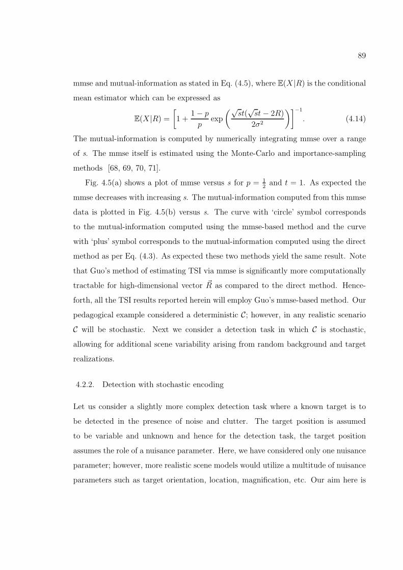
89
mmse and mutual-information as stated in Eq. (4.5), where E(X|R) is the conditional
mean estimator which can be expressed as
E(X|R) =
[1 +
1 − p
pexp
(√st(
√st− 2R)
2σ2
)]−1
. (4.14)
The mutual-information is computed by numerically integrating mmse over a range
of s. The mmse itself is estimated using the Monte-Carlo and importance-sampling
methods [68, 69, 70, 71].
Fig. 4.5(a) shows a plot of mmse versus s for p = 12
and t = 1. As expected the
mmse decreases with increasing s. The mutual-information computed from this mmse
data is plotted in Fig. 4.5(b) versus s. The curve with ‘circle’ symbol corresponds
to the mutual-information computed using the mmse-based method and the curve
with ‘plus’ symbol corresponds to the mutual-information computed using the direct
method as per Eq. (4.3). As expected these two methods yield the same result. Note
that Guo’s method of estimating TSI via mmse is significantly more computationally
tractable for high-dimensional vector ~R as compared to the direct method. Hence-
forth, all the TSI results reported herein will employ Guo’s mmse-based method. Our
pedagogical example considered a deterministic C; however, in any realistic scenario
C will be stochastic. Next we consider a detection task in which C is stochastic,
allowing for additional scene variability arising from random background and target
realizations.
4.2.2. Detection with stochastic encoding
Let us consider a slightly more complex detection task where a known target is to
be detected in the presence of noise and clutter. The target position is assumed
to be variable and unknown and hence for the detection task, the target position
assumes the role of a nuisance parameter. Here, we have considered only one nuisance
parameter; however, more realistic scene models would utilize a multitude of nuisance
parameters such as target orientation, location, magnification, etc. Our aim here is

90
T1 T2 TP
M2 P
=×
T2
1
0
0
T ~ρ T2
(a)
Vc2 VcK
M2 K
=×
Vc~β Vc
~β
Vc1
0.5
0.8
0.3
(b)
Figure 4.6. Illustration of stochastic encoding Cdet: (a) Target profile matrix T and
position vector ~ρ and (b) clutter profile matrix Vc and mixing vector ~β.
to demonstrate an application of the TSI framework and the extension to additional
nuisance parameters will be straightforward.
The imaging model for this task is constructed as
~R = HCdet(X) + ~N, (4.15)
where H is the imaging channel matrix operator, ~N is the zero-mean additive white
Gaussian detector noise (AWGN) with covariance Σ ~N and Cdet is the stochastic
encoding operator. The encoding operator Cdet is defined as
Cdet(X) =√sT~ρX +
√cVc
~β, (4.16)
where T is the target profile matrix, in which each column is a target profile (lexico-
graphically ordered into a one-dimensional vector) at a specific position in the scene.
In general, when the scene is of dimension M ×M pixels and there are P different
possible target positions, the dimension of matrix T is M2 × P . The column vector
~ρ is a random indicator vector and selects the target position for a given scene real-
ization. Therefore, ~ρ ∈ ~c1,~c2...~cP where ~ci is a P -dimensional unit column vector

91
with a 1 in the ith position and 0 in all remaining positions. Fig. 4.6(a) illustrates the
structure of T and ~ρ. Note that ~ρ = ~c2 in Fig. 4.6(a) and therefore the output of T~ρ
is the target profile at position 2. All positions are assumed to be equally probable,
therefore Pr(~ρ = ~ci)=1P
for i = 1, 2, ...P. The virtual source variable X takes the
value 1 or 0 (i.e. “target present” or “target absent”) with probabilities p and 1 − p
respectively.
Vc is the clutter profile matrix whose columns represent various clutter compo-
nents such as tree, shrub, grass etc. The dimension of Vc is M2 × K where K is
the number of clutter components. ~β is the K-dimensional clutter mixing column
vector, which determines the strength of various components that comprise the clut-
ter. ~β follows a multivariate Gaussian distribution with mean ~µ~β and covariance Σ~β.
Fig. 4.6(b) shows individual clutter components arranged column-wise in the clutter
profile matrix Vc. The particular realization of clutter mixing vector ~β shown in
Fig. 4.6(b) yields the clutter shown on the right-hand side.
The coefficient c in Eq. (4.16) denotes the clutter-to-noise ratio. Note that clutter
and detector noise combine to form a multivariate Gaussian random vector ~Nc =√cHVc
~β + ~N with mean ~µ ~Nc= ~µ~β and covariance Σ ~Nc
= HVcΣ~βVcTHT · c + Σ ~N .
Now, we can rewrite the imaging model as
~R =√sHT~ρX + ~Nc. (4.17)
The task-specific information for the detection task is the mutual-information
between the image measurement ~R and the virtual source X. Since the encoding
operator Cdet is a random function of the source X, we apply the result given in
Eq. (4.10). Comparing Eq. (4.10) with the imaging model shown in Eq. (4.17) we
note that the ~X and ~Y in Eq. (4.10) are equal to the virtual source X and T~ρX
respectively. The channel operator H is substituted by H and ~N is replaced by ~Nc

92
M2
=
P
0
0
0
1
0
0
1
0
T2 T2+P
TρT ρ
×
T1 T2 TP T1+P T2+P T2P
Figure 4.7. Structure of T and ρ matrices for the two-class problem.
in Eq. (4.10). The TSI and mmseH are therefore related as
TSI = I(X; ~R) =1
2
∫ s
0
mmseH(s′)ds′, (4.18)
where mmseH(s) = Tr(H†Σ−1~Nc
H(E~Y −E~Y |X)), (4.19)
and ~Y = T~ρX. (4.20)
Explicit expressions for the estimators required for evaluating the expectations in
Eq. (4.19) are derived in Appendix A.
4.2.3. Classification with stochastic encoding
We consider a simple two-class classification problem for which we label the two
possible states of nature (i.e., targets) as H1 and H2. The extension to more than
two classes is straightforward and is considered later. The overall imaging model
remains the same as in Eq. (4.15). The number of positions that each target can
take remains unchanged. However, now T has dimensions M2 × 2P and is given by
T = [TH1TH2
] where THiis the target profile matrix for class i. The structure of this
composite target profile matrix T is shown in Fig. 4.7. The virtual source variable is
denoted by the vector ~X and takes the values [1, 0]T or [0, 1]T to represent H1 or H2

93
respectively. The prior probabilities for H1 and H2 are p and 1− p respectively. The
vector ~ρ from the detection problem becomes a matrix ρ of dimension 2P × 2 and is
defined as
ρ =
[~ρH 00 ~ρH
], (4.21)
where ~ρH ∈ ~c1,~c2....~cP and 0 is an all zero P -dimensional column vector. Once
again we assume all positions to be equally probable, therefore Pr(~ρH = ~ci)=1P
for
i = 1, 2, .., P.Consider an example that illustrates how the term Tρ ~X enables selection of a
target from either H1 or H2 at one of P positions. In order to generate a target from
H1 at the mth position in the scene, ~ρH = ~cm and ~X = [1, 0]T . The product of Tρ
will produce a M2×2 matrix whose first column is equal to the H1 profile at position
m and whose second column is equal to the H2 profile at the same position. This
resulting matrix, when multiplied by ~X = [1 0]T , will select the H1 profile. Similarly,
in order to choose a target from H2 at the mth position, ~ρH = ~cm and ~X = [0 1]T .
Note that ~ρH = ~c2 in Fig. 4.7 and therefore, selects the second position for H1 and
H2.
The imaging model presented for the detection problem in Eq. (4.17) and the
corresponding TSI defined in Eq. (4.18) require minor modifications to remain valid
for the classification problem. Specifically, we require the virtual source variable
to become a vector quantity ~X, and the dimensions of T and ρ to be adjusted
accordingly, as noted above. Note that despite the increase in dimensionality, the
binary source vector ~X results in the upper bound TSI ≤ 1 bit for the two-class
classification problem.
The two-class model for target classification can easily be extended to the case of
joint detection and classification. The simple extension involves introducing a third
class corresponding to the null hypothesis and can be accommodated by allowing ~X
to also take the value [0 0]T with some probability p0. The TSI upper bound in this

94
M2
T
×
Region 4Region 3Region 2Region 1
0
01
00
0
0
0
00
P4
P
=1
0
0
0
Λ
Region 2
TΛ
Figure 4.8. Structure of T and Λ matrices for the joint detection/localization prob-lem.
case becomes J( ~X) = −p0 log(p0)− p1 log(p1)− p2 log(p2) ≤ 1.6 bits for p0 = p1 = p2.
This important extension to joint detection and classification is pursued further in
the next section, where we also consider the simultaneous estimation of an unknown
target parameter.
4.2.4. Joint Detection/Classification and Localization
We begin with a discussion of the localization task. Later in this section we combine
the encoding model for localization with the models for detection and classification
described in Subsections 4.2.2 and 4.2.3. Consider the problem of localizing a target
(known to be present) in one of Q regions in a scene. The example shown in Fig. 4.8
depicts a case in which there are four regions (Q = 4). Note that for this problem,
the specific target location within a region is unimportant and is therefore treated
as a nuisance parameter. We allow Pi possible target locations within the ith region
such that∑Q
i=1 Pi = P , where P is the total number of possible target locations in
the scene. The noise and clutter models remain unchanged from Subsections 4.2.2
and 4.2.3 so that the task-specific imaging model for localization can be written as
~R =√sHTΛ(X)~ρ+ ~Nc, (4.22)

95
where we have simply inserted the localization matrix Λ(X) into the channel model
in Eq. (4.17). As defined earlier, the columns of T correspond to the target profiles
at all possible positions. For the sake of convenience, we rearrange the columns of
T such that the first P1 columns represent the target profiles at the P1 positions
in region 1, the next P2 columns correspond to region 2, and so on. The virtual
source variable X is now a Q-ary variable i.e., X ∈ 1, 2, .., Q representing one of
the Q regions where the target is present. Λ(X) acts as the localization matrix and
selects all target profiles in the region specified by the source X. For the case X = i,
Λ(X = i) is of dimension P × Pi and given by
Λ(X = i) =
[0]P1×Pi
...[0]Pi−1×Pi
[I]Pi×Pi
[0]Pi+1×Pi
...[0]PQ×Pi
.
For X = i, ~ρ is a Pi-dimensional random indicator vector which selects one of the
Pi target profiles resulting from TΛ(X = i). Therefore, ~ρ ǫ ~e1, ~e2....~ePi where
~ek is a Pi-dimensional unit column vector with a 1 in the kth position and 0 in all
remaining positions. All positions within each region are considered to be equally
probable; therefore, Pr(~ρ = ~ek) = Pr(X=i)Pi
, where Pr(X = i) is the probability of the
target being located in region i and k = 1, 2, .., Pi. Fig. 4.8 illustrates the structure
of T and Λ(X) using an example where X = 2. In the example, P positions are
equally distributed among the 4 regions i.e., Pi = P4
for i = 1, 2, 3, 4. Observe
that TΛ(X) selects all the target positions in region 2 and the post-multiplication
of this matrix with ~ρ = ~ek results in the target at the kth position of region 2.
Recall that the localization task is only concerned with estimating the region in
which the target is present and the exact position within the region is treated as
a nuisance parameter. Therefore, the upper bound on TSI in this case becomes

96
Region 2
2P
=
Region 2
M2
Region 4Region 3Region 2Region 1
Region 1 Region 2 Region 3 Region 4T
2 × P4
Λ
0
0
Λ
×
Ω TΩ
Figure 4.9. Structure of T and Ω matrices for the joint classification/localizationproblem.
J(X) = −∑Qq=1 Pr(X = q) log Pr(X = q) ≤ [logQ ]bits.
We now combine the encoding model for localization, defined in Eq. (4.22), with
the detection and classification models described in the previous section. For the joint
detection/localization task we are interested in detecting the presence of a target and
if present, localizing it in one of Q regions. The imaging model from Eq. (4.22)
becomes
~R =√sHTΛ(X)~ρα + ~Nc, (4.23)
where α is a binary variable indicating the presence or absence of the target. There-
fore, the virtual source in this case is a (Q + 1)-ary variable and is defined as:
X ′ ∈ X, 0 so that when α = 0, X ′ = 0 and when α = 1, X ′ = X. Compar-
ing Eq. (4.10) with the imaging model shown in Eq. (4.23), we note that the ~X and
~Y in Eq. (4.10) are equal to the virtual source X ′ and the term TΛ(X)~ρα respectively.
The channel operator H is replaced with H and ~N is replaced by ~Nc. Therefore, TSI

97
and mmseH for this task can be expressed as
TSI = I(X ′; ~R) =1
2
∫ s
0
mmseH(s′)ds′, (4.24)
where mmseH(s) = Tr(H†Σ−1~Nc
H(E~Y −E~Y |X′)), (4.25)
X ′ ∈ X, 0 , ~Y = TΛ(X)~ρα. (4.26)
The (Q+1)-ary nature of the virtual source variable in the joint detection/localization
task increases the upper bound on TSI as compared to that for the simple detection
task. For the probabilities Pr(α = 1) = p and Pr(α = 0) = 1 − p, the TSI is upper
bounded by
J(X ′) = −(1 − p) log(1 − p) −Q∑
q=1
Pr(X = q) log Pr(X = q), (4.27)
where∑Q
q=1 Pr(X = q) = p. For the case of p = 12
and Pr(X = q) = pQ
, the maximum
TSI is [1 + 12logQ ]bits.
Finally, we consider the joint classification/localization task where the task of
interest is to identify one of the two targets from H1 or H2 and localize it in one of
Q regions. The exact position of the target within each region remains a nuisance
parameter. The imaging model for this task is given by
~R =√sHTΩ(X)ρ~α+ ~Nc. (4.28)
This model is the same as the one given in Eq. (4.23) except for minor modifications.
The total number of positions that each target can take remains unchanged. However,
now T has dimensions M2×2P and is given by T = [TH1TH2
] where THiis the target
profile matrix for target i. The arrangement of the target profiles in TH1and TH2
is
similar to the arrangement described in Subsection 4.2.3. The virtual source in this
case is 2Q-ary and given by ~X ′ = [X, ~α], where X ∈ 1, 2.., Q indicates the region
and ~α ∈ [1, 0]T , [0, 1]T represents one of the two targets. The localization matrix
Ω(X = i), now has dimensions 2P × 2Pi for selecting the H1 and H2 profiles in the

98
(a) (b)
(c) (d)
Figure 4.10. Example scenes: (a) Tank in the middle of the scene, (b) Tank in thetop of the scene, (c) Jeep at the bottom of the scene, and (d) Jeep in the middle ofthe scene.

99
region i and is given by
Ω(X = i) =
[Λ(X = i) 0
0 Λ(X = i)
], (4.29)
where matrices Λ(X = i) and 0 are of dimension P × Pi. The matrix Λ(X) is
identical to the one in Eq. (4.22). Fig. 4.9 illustrates the role of TΩ(X) in choosing
the H1 and H2 profiles at all positions in the region specified by X. This example
uses X = 2, Q = 4, and Pi = P4
for i = 1, 2, 3, 4. The matrix TΩ(X) in Eq. (4.28)
is post-multiplied by the matrix ρ of dimension 2Pi × 2 to yield the targets H1 and
H2 at one of the positions in region i. Here ρ is defined as
ρ =
[~ρH 00 ~ρH
], (4.30)
where 0 is an all zero Pi-dimensional column vector and ~ρH ∈ ~e1, ~e2....~ePi, where ~ek
is an indicator vector as before. Therefore, for ~ρH = ~ek, TΩ(X)ρ results in a M2 × 2
matrix with its first column representing H1 at the kth position in region i and its
second column representing H2 at this same position. This result is then multiplied
by ~α which selects either H1 or H2 for ~α = [1, 0]T or ~α = [0, 1]T respectively.
The TSI expression in Eq. (4.24) requires only minor modifications to remain valid
for the joint classification and localization problem. The upper bound for TSI in this
task is given by
J( ~X ′) = −2∑
i=1
P∑
q=1
Pr(X = q, ~αi) log Pr(X = q, ~αi), (4.31)
where ~α1 = [0, 1]T , ~α2 = [1, 0]T ,∑Q
q=1 Pr(X = q, ~α1) = 1 − p, and∑Q
q=1 Pr(X =
q, ~α2) = p. For the case when p = 12, Pr(X = q, ~α1) = 1−p
Qand Pr(X = q, ~α2) = p
Q,
the maximum TSI is [1 + logQ ]bits.
4.3. Simple Imaging Examples
The TSI framework described in the previous section allows us to evaluate the task-
specific performance of an imaging system for a task defined by a specific encoding

100
operator and virtual source variable. Three encoding operators corresponding to three
different tasks: (a) detection, (b) classification, and (c) joint detection/classification
and localization have been defined. Now we apply the TSI framework to evaluate
the performance of both a geometric imager and a diffraction-limited imager on these
three tasks.
We begin by describing the source, object, and clutter used in the scene model.
The source variableX in the detection task represents “tank present” or “tank absent”
conditions with equal probability i.e. p = 12. In the classification task, the source
variable ~X represents “tank present” or “jeep present” states with equal probability.
The joint localization task adds the position parameter to both the detection and
classification tasks. From Eq. (4.16) we see that the source parameter is the input
to the encoding operator, which in turn generates a scene consisting of both object
and clutter. Here the scene ~Y is of dimension 80 × 80 pixels (M = 80). The object
in the scene can be either a tank or a jeep at one of 64 equally likely positions
(P = 64). Therefore, the matrix T has dimensions of 6400 × 64 for the detection
task and 6400 × 128 for the classification task. In our scene model, the number of
clutter components is set to K = 6. Recall that the clutter components are arranged
as column vectors in the clutter matrix Vc. Clutter is generated by combining these
components with relative weights specified by the column vector ~β. Note that each
clutter vector is non-random but the weight vector ~β follows a multivariate Gaussian
distribution. In the simulation study the mean of ~β is set to ~µ~β = [160 80 40 40 64 40]
and covariance to Σ~β = ~µTβ I/5. The clutter to noise ratio, denoted by c, is set to 1.
The noise ~N is zero mean with identity covariance matrix Σ ~N = I.
Monte-Carlo simulations with importance sampling are used to estimate mmseH
using the conditional mean estimators for a given task. The mmseH estimates are
numerically integrated to obtain TSI over a range of s. For each value of s, we use
160, 000 clutter and noise realizations in the Monte-Carlo simulations.
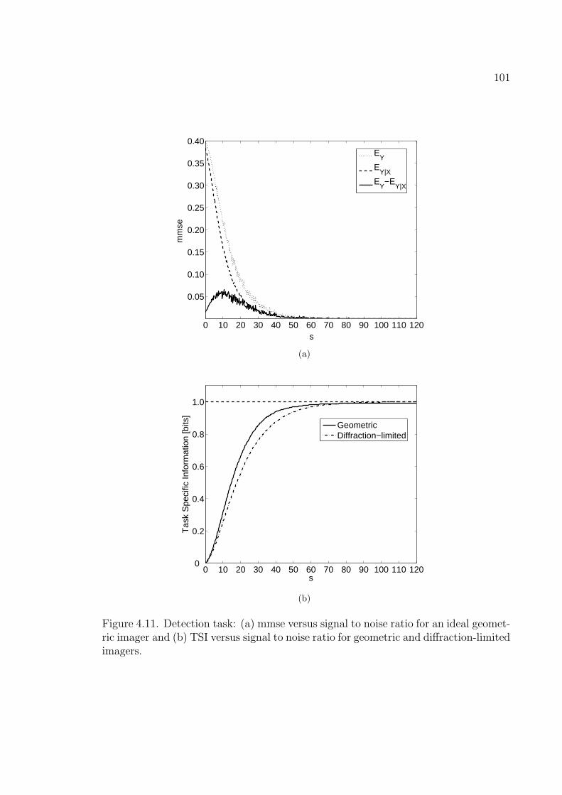
101
0 10 20 30 40 50 60 70 80 90 100 110 120
0.05
0.10
0.15
0.20
0.25
0.30
0.35
0.40
s
mm
se
EY
EY|X
EY−E
Y|X
(a)
0 10 20 30 40 50 60 70 80 90 100 110 1200
0.2
0.4
0.6
0.8
1.0
s
Tas
k S
peci
fic In
form
atio
n [b
its]
GeometricDiffraction−limited
(b)
Figure 4.11. Detection task: (a) mmse versus signal to noise ratio for an ideal geomet-ric imager and (b) TSI versus signal to noise ratio for geometric and diffraction-limitedimagers.

102
4.3.1. Ideal Geometric Imager
The geometric imager represents an ideal imaging system with no blur and therefore,
we set H= I. Fig. 4.10 shows some example scenes resulting from object realizations
measured in the presence of noise. Note that the object in the scene is either a tank
or a jeep at one of the 64 positions.
We begin by describing the results for the detection task. Fig. 4.11(a) and
Fig. 4.11(b) show the plots of mmseH and TSI versus s respectively. Recall that
the mmseH is equal to the difference of E~Y and E~Y |X represented by the dotted and
dashed curves in Fig. 4.11(a) respectively. The term E~Y |X represents the mmse in
estimating ~Y given the knowledge of both the measurement ~R and source X. There-
fore, we expect it to always be less than E~Y , which is the mmse in estimating ~Y
given only the measurement ~R. Fig. 4.11 confirms this behavior. In the low s region,
mmseH (in solid line) is small as both E~Y and E~Y |X are nearly equal. Despite the
additional conditioning on X, E~Y |X does not significantly improve upon E~Y as the
noise remains the dominating factor. However, in the moderate s region E~Y |X im-
proves faster than E~Y and therefore the mmseH increases here. In the high s regime,
the noise has negligible effect and hence the additional knowledge of X does not sig-
nificantly improve E~Y |X . This leads to the mmseH converging towards zero as both
the mmse components become equal. The solid line in Fig. 4.11(b) shows the plot
of TSI versus s. As expected the TSI increases with s eventually saturating at 1 bit.
The saturation occurs because TSI is always upper bounded by the entropy of the
virtual source X. The TSI plot confirms our expectations regarding blur-free imaging
system performance with increasing s.
Now we consider TSI for the joint task of detecting and localizing a target. The
scene is partitioned into four regions, i.e., Q = 4. There are a total of 64 allowable
target positions, with 16 positions in each region. Fig. 4.12 shows some examples
scenes. Recall that the position of the target within each region is a nuisance param-

103
(a) (b)
(c) (d)
Figure 4.12. Scene partitioned into four regions: (a) Tank in the top left region ofthe scene, (b) Tank in the top right region of the scene, (c) Tank in the bottom leftregion of the scene, and (d) Tank in the bottom right region of the scene.
eter. We assume that the probability of the target being present or absent is 12
and
the conditional probability of the target in any of the four regions is 14, given that the
target is present. The entropy of the source variable therefore, increases to 2 bits as
per Eq. (4.27). Fig. 4.13(a) shows a plot of mmse versus s for the joint detection and
localization task. The dotted line represents the mmse of the estimator conditioned
over the image measurement only. The dashed line corresponds to the mmse of the
estimator conditioned jointly on the virtual source variable and the image measure-
ment. As expected we see that E~Y |X ≤ E~Y . The solid line represents mmseH , the
difference between the dotted and dashed curves, and is integrated to yield TSI. The
TSI of the geometric imager is plotted in solid line versus s in Fig. 4.13(b) . We note
that the TSI saturates at 2 bits as expected.
The previous two examples have demonstrated how the formalism of Section 4.2

104
0 10 20 30 40 50 60 70 80 90 100 110 1200
0.05
0.10
0.15
0.20
0.25
0.30
0.35
0.40
s
mm
se
EY
EY|X’
EY−E
Y|X’
(a)
0 10 20 30 40 50 60 70 80 90 100 110 1200
0.4
0.8
1.2
1.6
2.0
s
Tas
k S
peci
fic In
form
atio
n [b
its]
GeometricDiffraction−limited
(b)
Figure 4.13. Joint detection/localization task: (a) mmse versus signal to noise ratiofor an ideal geometric imager and (b) TSI versus signal to noise ratio for geometricand diffraction-limited imagers.

105
can be applied to either a detection task or a joint detection/localization task. These
examples have also confirmed the two important TSI trends: (1) TSI is a monotoni-
cally increasing function of signal to noise ratio and (2) TSI saturates at the entropy
of the virtual source. Section 4.2 also described how a classification task or a joint
classification/localization task may be captured within the TSI formalism. The solid
curve in Fig. 4.14 depicts the TSI obtained from an ideal geometric imager for a
classification task in which the two classes are equally probable. Recall that for the
classification task we treat the position as the nuisance parameter and so the equi-
probable assumption results in a virtual source entropy of 1 bit. As expected the TSI
in Fig. 4.14 saturates at 1 bit. Fig. 4.15 presents the results of the TSI analysis of the
joint classification/localization task. Once again we have used two equally probable
targets and Q = 4 equally probable regions resulting in a source entropy of 3 bits. We
see that once again despite the measurement entropy that results from random clut-
ter and noise, the TSI provides an accurate estimate of the task-specific information,
saturating at 3 bits.
4.3.2. Ideal Diffraction-limited imager
The previous subsection presented the TSI results for an ideal geometric imager.
Those results should therefore be interpreted as upper bounds on the performance of
any real-world imager. In this subsection, we examine the effect of optical blur on TSI.
We will assume aberration-free, space-invariant, diffraction-limited performance. The
discretized optical point spread function (PSF) associated with a rectangular pupil
can be expressed as [29]
hi,j =
∫ ∆/2
−∆/2
∫ ∆/2
−∆/2
sinc2
((x− i∆)
W
)sinc2
((y − j∆)
W
)dxdy, (4.32)
where ∆ is the detector pitch and W quantifies the degree of optical blur associated
with the imager. Lexicographic ordering of this two-dimensional PSF yields one row
of H and all other rows are obtained by lexicographically ordering shifted versions of
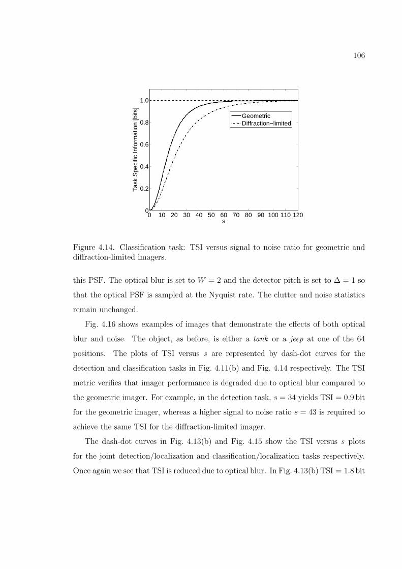
106
0 10 20 30 40 50 60 70 80 90 100 110 1200
0.2
0.4
0.6
0.8
1.0
s
Tas
k S
peci
fic In
form
atio
n [b
its]
GeometricDiffraction−limited
Figure 4.14. Classification task: TSI versus signal to noise ratio for geometric anddiffraction-limited imagers.
this PSF. The optical blur is set to W = 2 and the detector pitch is set to ∆ = 1 so
that the optical PSF is sampled at the Nyquist rate. The clutter and noise statistics
remain unchanged.
Fig. 4.16 shows examples of images that demonstrate the effects of both optical
blur and noise. The object, as before, is either a tank or a jeep at one of the 64
positions. The plots of TSI versus s are represented by dash-dot curves for the
detection and classification tasks in Fig. 4.11(b) and Fig. 4.14 respectively. The TSI
metric verifies that imager performance is degraded due to optical blur compared to
the geometric imager. For example, in the detection task, s = 34 yields TSI = 0.9 bit
for the geometric imager, whereas a higher signal to noise ratio s = 43 is required to
achieve the same TSI for the diffraction-limited imager.
The dash-dot curves in Fig. 4.13(b) and Fig. 4.15 show the TSI versus s plots
for the joint detection/localization and classification/localization tasks respectively.
Once again we see that TSI is reduced due to optical blur. In Fig. 4.13(b) TSI = 1.8 bit

107
0 10 20 30 40 50 60 70 80 90 100 110 1200
0.5
1.0
1.5
2.0
2.5
3.0
s
Tas
k S
peci
fic In
form
atio
n [b
its]
GeometricDiffraction−limited
Figure 4.15. Joint classification/localization task: TSI versus signal to noise ratio forgeometric and diffraction-limited imagers.
is achieved at s = 35 for the diffraction-limited imager as opposed to s = 28 in
case of the geometric imager for the detection/localization task. Similarly, for the
classification/localization task the signal to noise ratio required to achieve TSI =
2.7 bit increases by 10 due to the optical blur associated with the diffraction-limited
imager.
In this section, we have presented several numerical examples that demonstrate
how the TSI analysis can be applied to various tasks and/or imaging systems. The
results obtained herein are consistent with our expectations that (1) TSI increases
with increasing signal to noise ratio, (2) TSI is upper bounded by J(X), and (3)
blur degrades TSI. Although these general trends were known in advance of our
analysis, we are encouraged by our ability to quantify these trends using a formal
approach. In the next section we will use a TSI analysis to evaluate the target-
detection performance of two candidate compressive imagers.

108
(a) (b)
(c) (d)
Figure 4.16. Example scenes with optical blur: (a) Tank in the top of the scene, (b)Tank in the middle of the scene, (c) Jeep at the bottom of the scene, and (d) Jeep inthe middle of the scene.

109
X Y Z
SourceChannel
SceneH[ ]
EncodingC[ ]
Virtual Projection NoiseN[ ]
R
MeasurementP[ ]
F
Figure 4.17. Block diagram of a compressive imager.
4.4. Compressive imager
For task-specific applications (e.g. detection) an isomorphic measurement (i.e. a
pretty picture) may not represent an optimal approach for extracting TSI in the
presence of detector noise and a fixed photon budget. The dimensionality of the
measurement vector has a direct effect on the measurement signal to noise ratio [6].
Therefore, we strive to design an imager that directly measures the scene information
most relevant to the task while minimizing the number of detector measurements and
thereby increasing the measurement signal to noise ratio. One approach towards this
goal is to measure linear projections of the scene, yielding as many detector measure-
ments as there are projections. We refer to such an imager as a compressive imager,
sometimes also referred to as a projective/feature-specific imager. Fig. 4.17 shows
the imaging chain block diagram modified to include a projective transformation P.
For the compressive imager the measurement can be written as
R = N (P(H(C(X)))). (4.33)
We only consider discrete linear projections here, therefore the P operator is
represented by the matrix P. If we consider the detection task from Subsection 4.2.2
then the measurement model for the compressive imager can be written as
~R =√sPHT~ρX + ~N ′
c, (4.34)
where, ~N ′c =
√cPHVcβ + ~N.
The TSI and the mmseH expressions for the compressive imager are found by substi-

110
tuting PH for H in Eqs. (4.18)-(4.25) yielding
TSI ≡ I(X; ~R) =1
2
∫ s
0
mmseH(s′)ds′, (4.35)
where mmseH(s) = Tr(H†P†Σ−1~N ′
c
PH(E~Y − E~Y |X)) (4.36)
here ~Y = T~ρX and E~Y and E~Y |X are given earlier in Eq. (4.10).
Similarly for the joint detection/localization task from Subsection 4.2.4 the mod-
ified expressions for the imaging model and TSI are given by
~R =√sPHTΛ(X)~ρα + ~Nc, (4.37)
TSI ≡ I(X ′; ~R) =1
2
∫ s
0
mmseH(s′)ds′, (4.38)
where mmseH(s) = Tr(H†P†Σ−1~Nc
PH(E~Y −E~Y |X′)) (4.39)
here X ′ ∈ X, 0 and ~Y = TΛ(X)~ρα.
We consider compressive imagers based on two classes of projection: a) princi-
pal component projections and b) matched filter projections. Their performance is
compared with that of the conventional diffraction-limited imager.
4.4.1. Principal component projection
Principal component (PC) projections are determined by the statistics of the object
ensemble. For a set of objects O, the PC projections are defined as the eigenvectors
of the object auto-correlation matrix ROO given by
ROO = E(ooT ), (4.40)
where o ∈ O is a column vector formed by lexicographically arranging the elements
of a two-dimensional object. Note that the expectation is over all objects in the set
O. These PC projection vectors are used as rows of the projection matrix P∗. In
our numerical study, example objects in the set O are obtained by generating sample

111
0 10 20 30 40 50 60 70 80 90 100 110 1200
0.2
0.4
0.6
0.8
1.0
s
Tas
k S
peci
fic In
form
atio
n [b
its]
Diffraction−limitedProjective F=8Projective F=16Projective F=24Projective F=32
Figure 4.18. Detection task: TSI for PC compressive imager versus signal to noiseratio.
realization of random scenes with varying clutter levels, target strength and target
position. Here we use 10, 000 such object realizations to estimate ROO. The projection
matrix P∗ consists of F rows of length M2 = 6400, which are the eigenvectors of
ROO corresponding to the F dominant eigenvalues. To ensure a fair comparison of
the compressive imager with the diffraction-limited imager, we constrain the total
number of photons used by the former to be less than or equal to the total number
photons used by the latter. The following normalization is applied to P∗ to enforce
this photon constraint resulting in the projection matrix P,
P =1
csP∗, (4.41)
where the maximum column sum: cs = maxj
∑Fi=1 |P∗
ij|.Fig. 4.18 shows the TSI for this compressive imager plotted as a function of s for
the detection task. The dash-dot curve represents the TSI for the diffraction-limited
imager from Subsection 4.3.2. Note that the TSI for a compressive imager increases

112
0 10 20 30 40 50 60 70 80 90 100 110 1200
0.4
0.8
1.2
1.6
2.0
s
Tas
k S
peci
fic In
form
atio
n [b
its]
Diffraction−limitedProjective F=8Projective F=16Projective F=24Projective F=32
Figure 4.19. Joint detection/localization task: TSI for PC compressive imager versussignal to noise ratio.
as the number of PC projections F is increased from 8 to 24. This can be attributed
to the reduction in truncation error associated with increasing F . However, there
is also an associated signal to noise ratio cost with increasing F as we distribute
the fixed photon budget across more measurements while the detector noise variance
remains fixed. This effect is illustrated by the case F = 32, where the TSI begins
to deteriorate. This is especially evident at low signal to noise ratio. Notwithstand-
ing this effect, the PC compressive imager is seen to provide improved task-specific
performance compared to a conventional diffraction-limited imager, especially at low
signal to noise ratio. For example, the compressive imager with F = 24 achieves a
TSI = 0.9 bit at s = 18; whereas, the diffraction-limited imager requires s = 34 to
achieve the same TSI performance.
The TSI plot for the joint detection/localization task is shown in Fig. 4.19 for
both the compressive and diffraction-limited imagers. We see the same trends as in
Fig. 4.18. As before, a TSI rollover occurs at F = 32 due to the signal to noise ratio

113
trade-off associated with increasing F . In comparison with the diffraction-limited
imager which requires s = 35 to achieve TSI =1.8 bit, the compressive imager with
F = 24 achieves the same level of performance at s = 19.
Although we have shown that the PC compressive imager provides larger TSI
than the diffraction-limited imager we cannot claim that the PC projections are an
optimal choice. This is because PC projections seek to minimize the reconstruction
error towards the goal of estimating the whole scene [28], which is an overly stringent
requirement for a detection task. In fact, for a detection problem it is well known
that the generalized matched filter (MF) approach is optimal in terms of the Neyman-
Pearson criterion [47]. In the next section we present the TSI results for a matched
filter compressive imager.
4.4.2. Matched filter projection
For a detection problem in which both the signal and background are known, the gen-
eralized MF provides the optimal performance in terms of maximizing the probability
of detection for a fixed false alarm rate [47]. Recall that in our detection problem
the target position is a nuisance parameter that must be estimated implicitly. In
such a case, instead of a matched filter (e.g. correlator) we consider a set of matched
projections. Each matched projection corresponds to the target at a given position.
Therefore, the resulting compressive imager yields the inner-product between the
scene and the target at a particular position specified by each projection. Note that
compressive imaging in such a case is similar to an optical correlator except that in
an optical correlator the inner-product values are obtained for all possible shifts of
the target: our compressive imager will compute inner-products for only a subset of
these shifts.
The projection matrix P of the matched projection imager is defined as
P = TΣ−1~Nc, (4.42)

114
0 5 10 15 20 25 30 35 40 45 50 55 600
0.2
0.4
0.6
0.8
1.0
s
Tas
k S
peci
fic In
form
atio
n [b
its]
Diffraction−limitedProjective F=16Projective F=32Projective F=64
Figure 4.20. Detection task: TSI for MF compressive imager versus signal to noiseratio.
where T is the modified target profile matrix with each row corresponding to a target
profile at a specific position. The number of positions chosen is F and therefore, the
dimensions of the matrix T is F ×M2. The target positions for constructing T are
chosen such that they are equally spaced with some overlap between the profiles at the
adjacent positions. The target profile matrix T is post-multiplied by Σ−1~Nc
to account
for the effects of detector noise [47]. The dimensions of P are F ×M2. Therefore,
the compressive imager with projection P yields F measurements as opposed to M2
measurements as in the case of the diffraction-limited imager, where F << M2. As
in the previous section, the MF projection matrix P is normalized as per Eq. (4.41)
to allow for a fair comparison with the diffraction-limited imager.
Recall that the target can appear at one of the 64 possible positions, hence F = 64
is the maximum number of projections. Fig. 4.20 shows the plot of TSI versus s for
the MF compressive imager with F = 16, 32, and 64. As before, we see that TSI
increases with number of projections F . However, at F = 32 the TSI shows the

115
0 5 10 15 20 25 30 35 40 45 50 55 600
0.4
0.8
1.2
1.6
2.0
s
Tas
k S
peci
fic In
form
atio
n [b
its]
Diffraction−limitedProjective F=16Projective F=32Projective F=64
Figure 4.21. Joint detection/localization task: TSI for MF compressive imager versussignal to noise ratio.
rollover effect due to the signal to noise ratio cost associated with increasing F .
Ideally, we expect that the maximum TSI is obtained for F = 64, as it includes all
possible target positions. However, there is some overlap between the target profiles
at adjacent positions and so F ≤ 64 projections are sufficient to extract the detection-
task related information. Note that, in the absence of the photon-count constraint, a
choice of F = 64 would have indeed provided the highest TSI. As expected the MF
projection imager yields better performance compared to the PC projection imager.
For example, to achieve TSI = 0.9 bit the MF projections with F = 32 requires s = 17
compared to s = 23 for the PC projections.
The TSI versus s plot for the joint detection/localization task is shown in Fig. 4.21.
Similar to the detection task, we observe the rollover effect at F = 32. As expected,
TSI saturates at 2 bits at high signal to noise ratio. The MF compressive imager with
F = 32 offers improved performance achieving TSI = 1.8 bit at s = 8 compared to
s = 19 required by the PC projection imager.

116
(a) (b)
Figure 4.22. Example textures (a) from each of the 16 texture classes and (b) withinone of the texture class.
4.5. Extended depth of field imager
The depth of field (DOF) of a conventional imager refers to the range of object dis-
tances over which the optical PSF blur is within a pre-specified limit. The shallow
depth of field of a conventional imager can be a limitation in some applications such
as non-cooperative object recognition where the object cannot be easily confined to a
narrow range of imaging distances. In such a case, it is necessary to extend the depth
of field of the imager while minimizing the performance degradation. One method of
achieving an extended depth of field (EDOF) is to stop down the aperture (i.e. reduce
the diameter of aperture-stop) while keeping the effective focal length fixed. However,
this approach has a significant SNR penalty that severely degrades the imager per-
formance. An alternate method of achieving EDOF involves engineering the optical
PSF of the imager such that the resulting performance degradation is minimized. In
this section, we will consider a texture classification task to demonstrate the optical
PSF engineering approach for achieving EDOF using TSI as a design metric.
For the texture classification task our scene model is defined by the following

117
0 1 2 3 4 5 6 7 8 9 10 11 12 13 14 15 160
0.5
1.0
1.5
2.0
2.5
3.0
3.5
4.0
s
Tas
k S
peci
fic In
form
atio
n [b
its]
Wd=0/d
o=2.00m
Wd=1/d
o=2.20m
Wd=2/d
o=2.43m
Wd=3/d
o=2.72m
Wd=4/d
o=3.09m
Wd=5/d
o=3.58m
Figure 4.23. TSI versus signal to noise ratio at various values of defocus.
encoding operator Ctex
Y = Ctex( ~X) =√sTρ ~X, (4.43)
where T is a M2×LP dimension texture class matrix composed of L sub-matrices Tl
of size M2×L, each representing one of the L texture classes. Here s denotes the SNR.
Each texture class consists of P texture realizations with random magnitude scalings.
Within each texture class, the texture realization is considered to be a nuisance pa-
rameter, similar to the target position parameter in the two-class target classification
problem. Also note that the texture class matrix T has the same structure as the
two-class target matrix defined in subsection 4.2.3. The matrix ρ is a LP ×L dimen-
sion matrix, with the same definition as the ρ matrix appearing in subsection 4.2.3,
it selects a particular texture realization from each of the L texture classes at random
with uniform probability 1P. The source variable ~X is a L-dimensional unit column
vector that selects a particular texture class with uniform probability 1L. Here we
consider a 16 class (L = 16) texture classification problem where each class consists

118
0 1 2 3 4 50.5
1
1.5
2
2.5
3
3.5
4
Wd − Defocus
Tas
k S
peci
fic In
form
atio
n [b
its]
do − Object distance [m]
2.00 2.25 2.50 2.75 3.00 3.25 3.50
s=10
s=4
Figure 4.24. TSI versus defocus at s = 10 and s = 4 for the texture classificationtask.
of 16 (P = 16) different random texture realizations (M = 80). Fig. 4.22(a) shows an
example of texture from each of the 16 texture classes and Fig. 4.22(b) shows example
texture realizations that comprise one of the texture class. Note that for this task
the entropy of the source variable ~X is 4.0 bits (J( ~X) = log(L) bits) as all of the 16
texture classes are equally likely. Given the source model defined in Eq. (4.43) we
can express the image measurement ~R as
~R = HCtex( ~X) + ~N, (4.44)
where H is the M2×M2 imaging matrix and ~N is a M2×1 zero-mean additive white
Gaussian noise column vector with identity covariance matrix i.e. Σ ~N = I. The
conditional mean estimators E[~Y |~R] and E[~Y |~R, ~X] required for computing the TSI
for this imaging model remain the same as those derived for the two-class classification
problem considered in subsection 4.2.3, except that the number of classes is 16 instead
of 2.

119
pixels
pixe
ls
−16 −12 −8 −4 0 4 8 12 16
−16
−12
−8
−4
0
4
8
12
16
(a)
pixels
pixe
ls−16 −12 −8 −4 0 4 8 12 16
−16
−12
−8
−4
0
4
8
12
16
(b)
pixels
pixe
ls
−16 −12 −8 −4 0 4 8 12 16
−16
−12
−8
−4
0
4
8
12
16
(c)
pixels
pixe
ls
−16 −12 −8 −4 0 4 8 12 16
−16
−12
−8
−4
0
4
8
12
16
(d)
Figure 4.25. Optical PSF of conventional imager at (a) Wd = 0, (b) Wd = 3 andcubic phase-mask imager with γ = 2.0 at (c) Wd = 0, (d) Wd = 3.
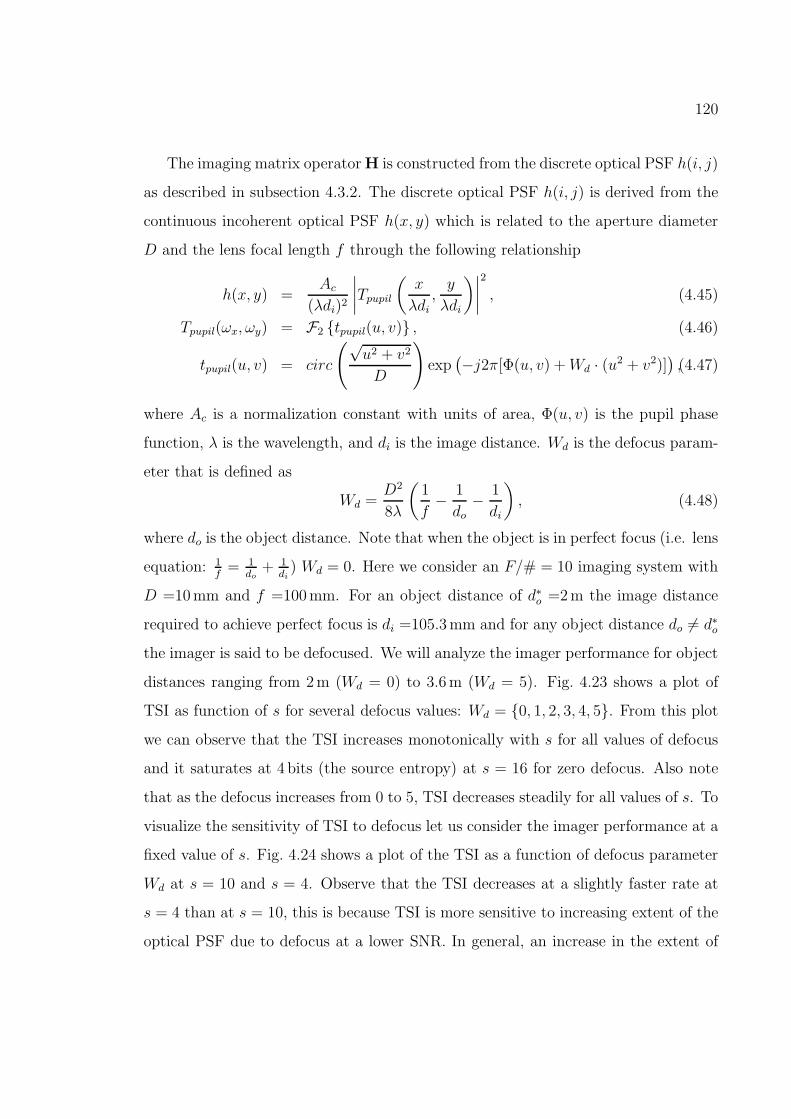
120
The imaging matrix operator H is constructed from the discrete optical PSF h(i, j)
as described in subsection 4.3.2. The discrete optical PSF h(i, j) is derived from the
continuous incoherent optical PSF h(x, y) which is related to the aperture diameter
D and the lens focal length f through the following relationship
h(x, y) =Ac
(λdi)2
∣∣∣∣Tpupil
(x
λdi,y
λdi
)∣∣∣∣2
, (4.45)
Tpupil(ωx, ωy) = F2 tpupil(u, v) , (4.46)
tpupil(u, v) = circ
(√u2 + v2
D
)exp
(−j2π[Φ(u, v) +Wd · (u2 + v2)]
),(4.47)
where Ac is a normalization constant with units of area, Φ(u, v) is the pupil phase
function, λ is the wavelength, and di is the image distance. Wd is the defocus param-
eter that is defined as
Wd =D2
8λ
(1
f− 1
do
− 1
di
), (4.48)
where do is the object distance. Note that when the object is in perfect focus (i.e. lens
equation: 1f
= 1do
+ 1di
) Wd = 0. Here we consider an F/# = 10 imaging system with
D =10mm and f =100mm. For an object distance of d∗o =2m the image distance
required to achieve perfect focus is di =105.3mm and for any object distance do 6= d∗o
the imager is said to be defocused. We will analyze the imager performance for object
distances ranging from 2m (Wd = 0) to 3.6m (Wd = 5). Fig. 4.23 shows a plot of
TSI as function of s for several defocus values: Wd = 0, 1, 2, 3, 4, 5. From this plot
we can observe that the TSI increases monotonically with s for all values of defocus
and it saturates at 4 bits (the source entropy) at s = 16 for zero defocus. Also note
that as the defocus increases from 0 to 5, TSI decreases steadily for all values of s. To
visualize the sensitivity of TSI to defocus let us consider the imager performance at a
fixed value of s. Fig. 4.24 shows a plot of the TSI as a function of defocus parameter
Wd at s = 10 and s = 4. Observe that the TSI decreases at a slightly faster rate at
s = 4 than at s = 10, this is because TSI is more sensitive to increasing extent of the
optical PSF due to defocus at a lower SNR. In general, an increase in the extent of

121
the optical PSF leads to a lower SNR per pixel and therefore, a lower TSI. Recall that
this “SNR cost” associated with the increasing extent of the optical PSF was also
observed in the case of the PRPEL imager design in Chapter 2. Thus, this SNR cost
is inherent to the optical PSF engineering approach irrespective of the task and/or
the design metric.
In order to quantify the depth of field of an imager we need to define a minimum
performance level/threshold. The range of object distances that maintain the imager
performance above this threshold define the depth of field of the imager. It is impor-
tant to emphasize that this criteria for depth of field definition is task-specific and
is also dependent on imager design specifications. For example, for reconstruction
tasks traditionally, the depth of field has been defined as the region within which the
optical PSF is smaller than a specified size. For a classification task, the depth of
field of an imager can be defined as the range of object distances for which the TSI
is above a threshold. Here we set this TSI threshold to 2 bits which is reached at a
defocus value Wd = 2.1 at s = 10. This defocus corresponds to an object distance of
2.46m yielding a depth of field of 46 cm. Note that this threshold is usually deter-
mined by the imager design specifications and here we have set it arbitrarily to 2 bits.
As mentioned earlier, engineering the optical PSF of an imager can extend its depth
of field. Here we will engineer the optical PSF by placing a cubic phase-mask in the
aperture-stop of the imager. The cubic phase-mask or the cubic pupil phase function
was originally derived in Ref. [4] to make the optical PSF invariant to defocus and
thereby extend the depth of field of an imaging system. It is defined as follows,
Φ(u, v) = γ · (u3 + v3) (4.49)
where γ is the parameter that controls the extent of defocus invariance of the resulting
optical PSF. Note that increasing γ, increases the defocus invariance of the optical
PSF however, it also reduces the imager performance as a result of a larger optical PSF
(larger extent) that leads to a lower SNR per pixel (the SNR cost). Fig. 4.25 shows the

122
0 0.25 0.50 0.75 1.00 1.25 1.50 1.75 2.00 2.25 2.50 45
50
55
60
65
70
75
80
85
90
γ
Dep
th o
f Fie
ld [m
m]
2.8
3.0
3.2
3.4
3.6
3.8
Tas
k S
peci
fic In
form
atio
n [b
its]
TSI at Wd=0
Depth of Field
γopt
=2.0
Figure 4.26. Depth of Field and TSI versus γ parameter at s = 10.
0 1 2 3 4 51.0
1.5
2.0
2.5
3.0
3.5
4.0
Wd − Defocus
Tas
k S
peci
fic In
form
atio
n [b
its]
Conventional
EDOF
DOF=46cm
DOF Threshold
DOF=81cm
Figure 4.27. TSI versus defocus at s = 10: DOF of conventional imager and cubicphase-mask EDOF imager with optimized optical PSF.

123
optical PSF with a cubic phase-mask (γ = 2) and the optical PSF without the cubic
phase-mask for two values of defocus Wd = 0 and Wd = 3. Note the larger extent of
the cubic phase-mask optical PSF relative to the conventional imager’s optical PSF
at zero defocus. The value of the parameter γ determines the imager’s depth of field
extension. Here we set the depth of field goal to 80 cm; the design problem can now
be stated as finding the value of γopt that achieves this goal. Fig. 4.26 shows a plot
of the depth of field and TSI (at focus) as a function of cubic phase-mask parameter
γ. From this plot we can observe that γopt = 2.0 achieves the desired depth of field
of 80 cm. Note that for this cubic phase-mask design with γopt = 2.0, the imager’s
performance at focus is however reduced to TSI = 3 bits. This performance penalty
represents the “cost” incurred in achieving the larger depth of field. Further, we
observe that this performance penalty increases monotonically with the increasing
depth of field, as the extent of the optical PSF increases with γ. Fig. 4.27 shows
the plot of TSI versus defocus parameter for both the conventional imager and the
optimized cubic phase-mask imager at s = 10. Note that the slope of the TSI curve is
lower for the cubic phase-mask imager compared to that for the conventional imager,
indicating a greater tolerance to defocus. It is important to emphasize that γopt and
therefore, the corresponding depth of field is function of SNR.
4.6. Conclusions
The task-specific information content of an image measurement can serve as an objec-
tive measure of the imaging system performance. In this chapter, we have proposed
a framework for the definition of TSI in terms of the well known Shannon mutual
information measure. The use of the virtual source variable is key to our definition
of TSI and to our knowledge, a unique method of embedding task specificity in the
scene model itself. The recently discovered relationship between mutual information
and mmse allows us to calculate the TSI from the simulated performance of con-

124
ditional mean estimators. The proposed TSI framework is applied to evaluate the
performance of geometric and diffraction-limited imaging systems for three tasks: de-
tection, classification and joint detection/classification and localization. The results
obtained from the simulation study confirm our intuition about the performance of
these two candidate imaging systems, thereby establishing TSI as an effective task-
specific performance metric.
We also exercised the TSI framework to study the design of two compressive im-
agers and an EDOF imager. In the case of the PC compressive imager, we found that
the TSI analysis confirmed the previously known trade-off with increasing number of
projections. The TSI performance of the MF compressive imager verified that it can
be a superior compressive imager design for a detection task. For the texture classifi-
cation task, we used TSI as a design metric to extend the depth of field of the imager
by nearly two times by engineering its optical PSF. From these results we conclude
that TSI is a useful metric for studying the task-specific performance of an imaging
system. We note that TSI may serve as an upper bound on the performance of any
algorithm that attempts to extract task-specific information from the measurement
data. In the next chapter we extend the application of the TSI metric to compressive
imaging system design and optimization.

125
Chapter 5
Compressive Imaging System Design With Task
Specific Information
In the last chapter, we used the TSI metric to analyze the task-specific performance
of two compressive imaging systems as a function of the number of projections to
understand the associated performance trade-offs. In this chapter, we extend this
study to the design of compressive imaging systems for the task of target detection.
We develop a TSI-based optimization framework to maximize the task-specific per-
formance of a compressive imaging system while accounting for the various physical
constraints such as the total photon count.
5.1. Introduction
Many modern applications of imaging involve some computational task. For exam-
ple, detection/classification and estimation tasks are commonly encountered in both
medical and military imaging applications. As discussed in Chapter 1, the tradi-
tional approach for designing such imaging systems involves at least two separate
steps: 1) design the front-end optical imaging system to maximize the fidelity of the
image measured at the detector plane and 2) design an algorithm that operates on
the measured image to extract the relevant information. This approach demonstrates
a disconnect between the task for which the acquired imagery is intended (e.g. de-
tection/estimation) and the imaging system design method that strives to achieve
the maximum image fidelity irrespective of the task. The computational imaging
paradigm addresses this disconnect through a joint optimization of the optical and
processing sub-systems [76, 77, 78, 79]. In this chapter, we are interested in a spe-
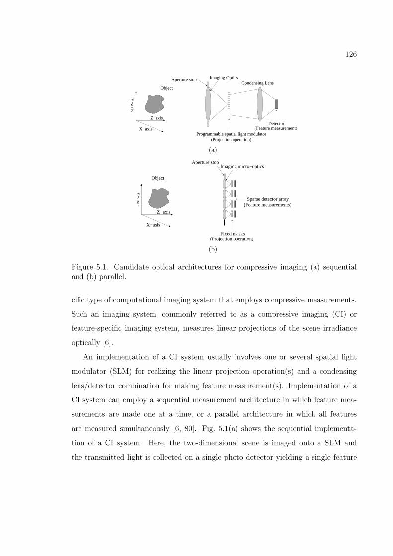
126
Condensing LensAperture stop Imaging Optics
(Projection operation)Programmable spatial light modulator
Object
Z−axis
X−axis
Y−
axis
Detector(Feature measurement)
(a)
Object
Z−axis
X−axis
Y−
axis
Aperture stopImaging micro−optics
Sparse detector array(Feature measurements)
Fixed masks(Projection operation)
(b)
Figure 5.1. Candidate optical architectures for compressive imaging (a) sequentialand (b) parallel.
cific type of computational imaging system that employs compressive measurements.
Such an imaging system, commonly referred to as a compressive imaging (CI) or
feature-specific imaging system, measures linear projections of the scene irradiance
optically [6].
An implementation of a CI system usually involves one or several spatial light
modulator (SLM) for realizing the linear projection operation(s) and a condensing
lens/detector combination for making feature measurement(s). Implementation of a
CI system can employ a sequential measurement architecture in which feature mea-
surements are made one at a time, or a parallel architecture in which all features
are measured simultaneously [6, 80]. Fig. 5.1(a) shows the sequential implementa-
tion of a CI system. Here, the two-dimensional scene is imaged onto a SLM and
the transmitted light is collected on a single photo-detector yielding a single feature

127
measurement. In order to obtain multiple feature measurements, the programmable
SLM is stepped through a sequence of projection vectors and the corresponding fea-
ture measurements are obtained as a time-sequence from the detector. Photons may
be allocated uniformly or non-uniformly among feature measurements through proper
choice of integrations times. In contrast to the sequential approach, the parallel archi-
tecture employs a lenslet array, fixed masks, and a sparse array of detectors to acquire
multiple feature measurements simultaneously as shown in Fig. 5.1(b). Once again
photons may be allocated uniformly or non-uniformly among feature measurements
through proper choice of lenslet apertures. This architecture has several advantages
as compared to the sequential architecture, including (a) reduced detector bandwidth
resulting in reduced noise, (b) elimination of the time-varying SLM, thus removal
of the attendant practical device limitations (e.g., photon loss due to imperfect fill
factor, contrast, and/or latency), and (c) potential for realizing extremely compact
CI imagers.
Linear feature-based techniques have been extensively studied by the image pro-
cessing community for target detection/classification and reconstruction tasks [81,
82, 83, 84]. The recent emergence of CI systems has been inspired by the incor-
poration of these linear feature-based techniques within the computational imaging
paradigm. There have been several studies characterizing the performance of vari-
ous CI systems [6, 80, 85, 86, 87, 88, 89, 90, 91]. Neifeld et al. [6, 80, 85, 86] and
Baraniuk et al. [90, 91] have studied CI for both reconstruction and detection tasks
and have discussed various potential advantages of the CI approach. A measure of
task-specific performance is important within the computational imaging framework.
Metrics such as visually-weighted root mean square error (RMSE) and probability
of detection/misclassification have been previously used to quantify the task-specific
performance of imaging systems [6, 86, 91]. However, an information-theoretic metric
is particularly attractive as it allows us to upper-bound the task-specific performance
of an imager, independent of the algorithm used to extract the relevant informa-

128
tion. In Chapter 4 we have developed a rigorous framework to define a task-specific
information-theoretic metric which we refer to as task-specific information. Task-
specific information (TSI) is based on the Shannon mutual-information measure and
it quantifies the task-relevant information available in an optical measurement. An
important observation regarding the information-theoretic nature of the TSI metric
is that the data processing inequality [67] dictates that the TSI cannot be increased
by any post-processing algorithm that operates on the measurement. This implies
that maximizing the TSI maximizes the upper-bound on the performance of any pro-
cessing algorithm and therefore, maximizes a CI system’s task-specific performance.
The relationship between Shannon information and estimation theory developed in
Refs. [73, 75, 92] facilitates the evaluation of TSI in a computationally tractable man-
ner. The utility of the TSI metric for evaluating the performance of both compressive
and conventional imagers for a variety of tasks has been demonstrated in Chapter 4. It
was found that the task-specific performance of compressive imagers can be superior
to that of conventional imagers, especially at low signal-to-noise ratio (SNR) [85].
In this chapter, we describe a method for TSI-based CI system design optimiza-
tion. We present a framework within which task-specific projections may be defined
and we demonstrate the utility of this framework by use of a specific target detection
problem. The target-detection task considered here includes the presence of nuisance
parameters, stochastic clutter, and detector noise. Numerous linear feature-based
techniques for target detection/classification exist in the literature. Projection bases
commonly employed by these techniques include, principal components [81, 82, 86],
independent components [83], wavelet bases [86], the Fisher basis [82] and random
projections [90, 91]. However, these projection bases have been developed for conven-
tional imagery (i.e. they are typically employed in the post-processing step that op-
erates on a conventional image). A direct optical implementation of these projection
bases in a CI system is therefore not optimal, as they do not account for parameters
like finite measurement SNR, clutter-to-noise-ratio (cnr), and the transfer function

129
3
4
1
5
2
Y Z
SourceChannel
H[ ]Encoding
C[ ]Virtual Projection Noise
N[ ]
R
P[ ]
FX
[0,1]
Image Feature MeasurementScene Feature
3.1
4.3
1.2
4.7
1.7
Figure 5.2. Block diagram of a compressive imaging system.
of the front-end optical system. We extend the TSI framework developed in Chapter
4 so that we may optimize CI systems while taking these various parameters into
account. We exploit the scene and target models developed in Chapter 4 to define
the target-detection task. The steps involved in our TSI-based design/optimization
framework are: 1) select a projection basis, and 2) optimize the total photon-budget
distribution among the various feature measurements. We analyze the task-specific
performance of the optimized CI system designs at various values of SNR and for a
variety of projection bases. The relationship between the probability of error and the
TSI-based detection-theoretic upper bound derived via Fano’s inequality [67] is also
examined.
5.2. Task-specific information: Compressive imaging system
Consider the various components of a CI system as illustrated in Fig. 5.2. The two-
dimensional scene Y is imaged through the imaging channel, denoted by the operator
H. The resulting two-dimensional image Z is optically projected onto a pre-defined
basis, to yield a feature vector denoted by F . The optical projection is represented
by the linear operator P. Finally, the feature vector F is corrupted by the noise
operator N resulting in the detector measurement R = N (F ). Task-specificity is
incorporated into this imaging system model by introducing a virtual source variable
and an encoding block. The virtual source variable, denoted by X, represents the
parameter(s) of interest for a specific task. For example, in a detection task X will be

130
a binary variable taking the values 1/0 representing target present/absent conditions.
In a reconstruction/estimation task, X might instead be a coefficient vector that
represents the scene of interest in some sparse basis. The encoding operator C operates
on X to produce the scene Y . In general, C can be either deterministic or stochastic.
TSI is defined as the Shannon mutual-information I(X;R) between the virtual
source X and the measurement R as follows [67]
TSI ≡ I(X;R) = J(X) − J(X|R), (5.1)
where J(X) = −Elog(pr(X)) denotes the entropy of the virtual sourceX, J(X|R) =
−Elog(pr(X|R)) denotes the entropy of X conditioned on the measurement R,
E· denotes the statistical expectation operator, pr(·) denotes the probability den-
sity function, and all logarithms are taken to be base 2. From this definition, it is
clear that the maximum TSI content of any measurement R is upper bounded by
the entropy of X. From here onwards we will assume that: 1) the channel opera-
tor H is linear, discrete-to-discrete, and deterministic, 2) the encoding operator C is
linear and stochastic, 3) the projection operator P is linear, discrete-to-discrete, and
deterministic, and 4) the noise model N is additive and Gaussian distributed.
5.2.1. Model for target-detection task
We consider a target-detection task, in which the target is known and background
clutter is stochastic. The target position is assumed to be variable and unknown.
Thus, the target position is a nuisance parameter. For this task, the virtual source
variableX takes the value 1 or 0 (i.e. “target present” or “target absent” respectively)
with probability p and 1−p respectively. In our scene model, the stochastic encoding
matrix operator C is defined as
C(X) =√sT~ρX +
√cVc
~β, (5.2)

131
where T is the target profile matrix, in which each column is a target profile (lexico-
graphically ordered into a one-dimensional vector) at a specific position in the scene.
For a scene of dimension M ×M pixels with P different possible target positions,
the dimension of the matrix T is M2 × P . The position vector ~ρ is a random indi-
cator vector that selects the target position for a given scene realization. Therefore,
~ρ ∈ ~c1, · · · ,~cP where ~ci is a P -dimensional vector with 1 at the ith position and
zeros elsewhere. All target positions are assumed to be equally probable. The clutter
profile matrix Vc is composed of column vectors that represent the various clutter
components such as tree, shrub, grass, etc. The dimension of Vc is M2 × L, where
L denotes the number of clutter components. ~β is the L-dimensional clutter mixing
column vector that follows a multivariate Gaussian distribution with mean ~µ~β and
covariance Σ~β . Fig. 5.3 illustrates the stochastic encoding operator C through an
example. Note that ~ρ = ~c2 in Fig. 5.3(a) and therefore, the output of T~ρ is the target
profile at position 2. Fig. 5.3(b) shows the individual clutter components arranged
column-wise in the clutter profile matrix Vc. The coefficients s and c in Eq. (5.2)
denote the signal-to-noise ratio (SNR) and clutter-to-noise ratio (CNR) respectively.
We note that this scene model is an oversimplified representation of the scenes typi-
cally encountered in practice. However, in the present work this model will serve to
illustrate the TSI-based design approach. A more realistic scene model would allow
for greater target variability in terms of orientation, illumination, perspective, and
a non-additive target/background model [93, 94, 95]. Furthermore, a more realistic
background clutter model would incorporate a varying number of clutter components
with variable positions, illumination, and perspectives. Although it would add numer-
ical complexity, such a model would not have any effect on the TSI-based optimization
methodology described herein.
The goal of the CI system in this work is to make K ≪ M2 measurements that
are most relevant to the detection-task. Mathematically, we can express the K-

132
T1 T2 TP
M2 P
=×
T2
1
0
0
T ~ρ T2
(a)
Vc2 VcL
M2 L
=×
Vc~β Vc
~β
Vc1
0.5
0.8
0.3
(b)
Figure 5.3. Illustration of stochastic encoding C: (a) Target profile matrix T and
position vector ~ρ and (b) clutter profile matrix Vc and mixing vector ~β.

133
dimensional detector measurement ~R as
~R = PHC(X) + ~N, (5.3)
where H is the M2 × M2 dimensional imaging channel matrix operator, P is the
K × M2 projection matrix operator, ~N is the K × 1 dimensional additive white
Gaussian detector noise (AWGN) vector with zero-mean and covariance Σ ~N , and C
is the stochastic encoding operator defined in Eq. (5.2). Note that the clutter and
the detector noise can be jointly described by a multivariate Gaussian random vector
~Nc as
~Nc =√cPHVc
~β + ~N, (5.4)
with mean ~µ ~Nc=
√cPHVc~µ~β and covariance Σ ~Nc
=√c ·PHVcΣ~βVc
THTPT +Σ ~N .
Therefore, we can rewrite the imaging model from Eq. (5.3) as
~R =√sPHT~ρX + ~Nc. (5.5)
Note that for a conventional imaging system (P = I), s refers to the measurement
SNR: the ratio of average signal power (s) measured on a detector to the detector
noise power σ2~Ni
= 1 and therefore, SNR = s. However, in the case of a CI system,
the detected signal power is increased by a factor of ‖~Pi‖2 as a result of the inner
product with projection vector ~Pi while the detector noise power remains fixed. This
results in a higher measurement SNR = s‖~Pi‖2 than that of a conventional imaging
system for the same value of s. To avoid ambiguity, from here onwards all references
to the term SNR will refer to the value of the s parameter.
To compute the mutual-information we will use the results derived in Refs. [73, 75,
85] that relate it to minimum mean square error (mmse) estimates. The relationship
between mutual information and mmse can be expressed as
TSI =1
2
∫ s
0
mmse(s′)ds′, (5.6)
where mmse(s) = Tr(H†P†Σ−1~Nc
PH(E~Y (s) −E~Y |X(s))). (5.7)

134
Here ~Y = T~ρX and
E~Y (s) = E[(~Y − E(~Y |~R, s))(~Y − E(~Y |~R, s))T ],
E~Y |X(s) = E[(~Y − E(~Y |~R,X, s))(~Y − E(~Y |~R,X, s))T ]. (5.8)
The terms E(~Y |~R, s) and E(~Y |~R,X, s) represent the conditional estimators for ~Y ,
with the former one conditioned over ~R and the latter one conditioned over both ~R and
X. Explicit expressions for these estimators, required for evaluating the expectations
in Eq. (5.8), can be found in Appendix A. Note that the relation between TSI and
mmse specified in Eq. (5.7) suggests that TSI increases with increasing mmse which
is counterintuitive. However, note that the actual mmse expression in Eq. (5.7) is
composed of two individual mmse terms E~Y and E~Y |X . The first mmse term E~Y is
the expected error in estimating ~Y given the measurement ~R, while the second mmse
term E~Y |X denotes the expected error given the joint knowledge of both ~R and X.
Fig. 5.4 shows a plot of these two mmse terms along with the difference mmse as a
function of SNR for a conventional imager. Note that in the low SNR region the two
mmse terms have similar values as the additional knowledge of X does not improve
the error significantly because the noise dominates in this region. In the mid SNR
region, the effect of noise is reduced and therefore, the second mmse error is lower
leading to an increase in difference mmse. The two mmse terms converge in the the
high SNR region as the noise becomes negligible with increasing SNR thereby making
the difference mmse smaller. Given that it is the difference between these mmse terms
whose integral is equal to TSI, it is expected that increasing the difference mmse leads
to a higher TSI. Note that TSI can not be increased arbitrarily by simply increasing
the difference mmse because the integral of the difference mmse is upper-bounded by
the entropy of the source variable X.

135
0 10 20 30 40 50 60 70 80 90 100 110 120
0.05
0.10
0.15
0.20
0.25
0.30
0.35
0.40
s
mm
se
EY
EY|X
EY−E
Y|X
Figure 5.4. Difference mmse and mmse components versus SNR for a conventionalimager.
5.2.2. Simulation details
The source variable X in our detection task represents “tank present” or “tank ab-
sent” conditions with equal probability i.e. p = 12. Here we consider a scene of
dimension 80× 80 pixels (i.e. M = 80). The object in the scene is a “tank” at one of
P = 64 equally likely positions and therefore, the matrix T is of dimensions 6400×64.
In our scene model, the number of clutter components is set to L = 6 with the L2
norm of each column vector in Vc set to unity. The mean of the mixing vector ~β is
set to ~µ~β = [160 80 40 40 64 40] and covariance to Σ~β = ~µTβ I/5. The CNR is set to
c = 1 and the detector noise ~N is AWGN with zero-mean and covariance Σ ~N = I.
We assume that the imaging optics in Fig. 5.1 (b) exhibits aberration-free, space-
invariant, and diffraction-limited performance for each lenslet. The discretized optical
point spread function (PSF) associated with a rectangular pupil therefore assumes

136
(a) (b)
Figure 5.5. Example scenes with optical blur and noise: (a) Tank in the top of thescene, (b) Tank in the middle of the scene
the following form [29]
h(i, j) =
∫ ∆/2
−∆/2
∫ ∆/2
−∆/2
sinc2
((x− i∆)
W
)sinc2
((y − j∆)
W
)dxdy, (5.9)
where W quantifies the degree of optical blur associated with the imaging optics and
∆ is the pixel pitch of the mask in Fig. 5.1(b). The optical blur is set to W = 2 and
the pixel pitch is set to ∆ = 1 so that the optical PSF is sampled at the Nyquist rate.
Note that a lexicographic ordering of the two-dimensional PSF yields one row of H
and all other rows are obtained by lexicographically ordering the appropriately shifted
version of this PSF. Fig. 5.5 shows example images that demonstrate the effects of
both optical blur and noise.
To ensure a fair comparison between CI and conventional imaging, we introduce
a system constraint based on the total photon-count. This system constraint has two
physical implications: 1) the total number of photons incident on the detector array
is always less than or equal to the total number of photons entering the entrance pupil
(i.e., the CI system is passive) and 2) the total number of photons available at the
entrance pupil is fixed (i.e., the CI system uses the same pupil and observation time
as the conventional imager). Mathematically, this total photon-count constraint can

137
be expressed as
P =1
ωP∗, (5.10)
where ω = maxj
∑Ki=1 |P∗
ij| denotes the maximum absolute column sum of the
matrix operator P∗. Here P∗ represents the original unnormalized projection matrix
and P refers to the normalized photon-count-constrained matrix that is implemented
optically. Note that a conventional imager does not employ a SLM and instead uses a
sensor array for image measurement, both P and P∗ are equal to an identity matrix
of dimension M2 ×M2.
Monte-Carlo simulations with importance sampling [68] are used to estimate the
mmse via the conditional mean estimators defined in Eq. (5.8). For each value of
s, 8000 clutter and noise realizations are used to estimate the mmse. These mmse
estimates are then numerically integrated with respect to SNR over the interval [0, s],
via the adaptive Lobatto quadrature method [96], to yield the TSI at s.
5.3. Optimization framework
We now describe the optimization framework for designing a CI system to maximize
task-specific performance. The degrees of freedom available in a CI system include
all the elements comprising the projection matrix P (i.e. all elements of P are valid
design variables). The constrained optimization problem can therefore be expressed
as
maxP
[TSI], such that maxj
K∑
i=1
|Pij| = 1. (5.11)
However, we note that the computational complexity resulting from the use of TSI
as a design metric increases exponentially with the number of design variables (which
is equal to K ×M2). As a result, this optimization approach becomes computation-
ally intractable for realistic scene dimensionality. Therefore, we pursue an alternate
approach that attempts to find the optimal photon-allocation per feature for a given

138
projection basis. This approach reduces the number of design parameters fromK×M2
to K, and therefore lowers the computational burden to a manageable level. We ex-
pect a TSI improvement through non-uniform photon-allocation scheme because, the
photon-budget can now be distributed among the basis vectors according to their
task-relevance. Note that in this approach the projection basis is pre-determined and
not optimized.
Within this optimization framework, the fraction of photons associated with the
ith basis vector ~Pi
∗(i.e. the ith row of P∗) is denoted by the design variable πi.
Therefore, for a given projection basis P∗ there is an associated photon-allocation
vector ~π that is defined as ~π = [π1, π2, · · · , πK ]. Note that the non-uniform photon
allocation vector ~π can be implemented via the use of non-uniform lenslet diameters in
the parallel CI architecture. Designing a CI system within the proposed optimization
framework involves three steps: 1) construct the unnormalized projection matrix
P∗ = [~P ∗1 ,~P ∗
2 , · · · , ~P ∗K ]T by choosing K projection vectors from the pre-defined basis,
2) construct the normalized projection matrix P = diag(~π)P∗ by choosing a ~π that
satisfies the photon-count constraint, where diag(·) denotes a diagonal matrix whose
diagonal is equal to its vector argument, and 3) optimize upon the associated photon-
allocation vector ~π in the presence of the total photon-count constraint to maximize
the TSI for a given value of SNR. Mathematically, this constrained optimization
problem can be expressed as
max~π
[TSI], such that maxj
K∑
i=1
|[diag(~π)P∗]ij | = 1. (5.12)
We use an optimization algorithm based on simulated tunneling [56] to maximize
the TSI for a given value of s. The simulated tunneling approach guarantees conver-
gence to the global maximum/minimum of an optimization problem as the number
of iterations tends to infinity. We observe convergence to a common solution after
5000 iterations, from multiple different initial conditions giving confidence that our

139
TSI optimization framework results in a global optima. Note that the computational
complexity of each iteration step is a function of the number of target positions P , the
number of projection vectors K, the SNR parameter s and the number of clutter/noise
realizations NCN used in the Monte-Carlo simulation. The number of floating points
operations (Flops) involved in each evaluation of the objective function can be ex-
pressed as ⌊√
10s⌋NCN(2P 4 + 2P 3 + 3P 2 + PK). For example, at s = 5, K = 1,
NCN = 8000 and P = 64, 1778GFlops were required to compute the TSI. Therefore,
as the number of target positions P is increased the computational cost grows quar-
tically O(P 4). Some practical tricks could be employed for large values of P like 1)
Monte-Carlo simulations over the diverse perspectives (only), and 2) parametrization
of the target library with P ≪ P parameters. However, it is important to realize that
the actual target detection problem does not become more complex as P increases
(for the same number of measured features) [84]. As mentioned earlier, several differ-
ent projection bases are considered for use in the CI system design. Now we describe
each of these projection bases in the context of our target-detection task.
5.3.1. Principal component projections
Principal component (PC) projections are derived from principal component analysis,
and are frequently employed for data dimensionality reduction in pattern recognition
problems [81]. The salient aspect of this basis is its strong energy compaction property
that leads to dimensionality reduction with the smallest reconstruction RMSE for
certain types of signals [97, 98]. The normally distributed signals fall in this category.
In practice, PC projections are computed using second-order statistics of a training
set chosen to represent an object ensemble. Specifically, for a training set O, the PC
projections are defined as the eigenvectors of the object auto-correlation matrix ROO
defined as
ROO = E~o~oT, (5.13)

140
Figure 5.6. Example projection vectors in the PC projection basis, clockwise fromupper left, #2,#6,#16,#31.
where ~o ∈ O is a column vector formed by lexicographically arranging the elements of
a two-dimensional image in O. Note that the expectation, denoted by operator E·,is over the complete training set O. In this work the object samples in the training
set O were obtained by generating sample realizations of scenes with varying clutter
levels, target strength, and target position using the stochastic encoder C defined in
Eq. (5.2). The K dominant eigenvectors of ROO are used to create the projection
matrix P∗PC. Fig. 5.6 shows some example projection vectors from this PC projection
basis.
In Chapter 4, it was demonstrated that the PC compressive imager, with an
uniform photon-allocation, achieves a higher TSI than that of the conventional imager.
This is the result of a higher measurement fidelity in a PC compressive imager due to
its strong image-energy compaction property. Fig. 5.7 shows the plot of TSI versus s
for the PC compressive imager for various choices of K. Observe that TSI increases

141
0 2 4 6 8 10 12 14 16 18 20 22 240
0.1
0.2
0.3
0.4
0.5
0.6
0.7
0.8
0.9
1.0
s
Tas
k−sp
ecifi
c In
form
atio
n [b
its]
K=12
K=16
K=24
K=32
Optimized
Figure 5.7. TSI versus SNR for PC compressive imager.
monotonically with s, eventually saturating at 1.0 bit. Also note that for a particular
SNR, TSI increases with K up to a certain value and then starts decreasing. We refer
to this behavior as the “rollover effect,” which is the result of a trade-off between
two competing processes: 1) as K increases, the projective measurements provide
more target-detection information, leading to an increase in TSI and 2) with a fixed
photon-budget, the measurement fidelity per feature decreases with increasing K,
resulting in a decrease in TSI. The tradeoff between these two processes results in
an optimal value of K that maximizes the TSI for a given value of SNR. For the
example in Fig. 5.7, the optimal value of K is 24 for s = 20. Note that the optimal
K is a function of SNR. From here onwards, we will refer to this effect of decreasing
measurement fidelity with increasing K as the “noise cost.”
In the next section we will further improve the PC compressive imager performance
by using the optimal photon-allocation. A PC projection matrix with K = 32 is
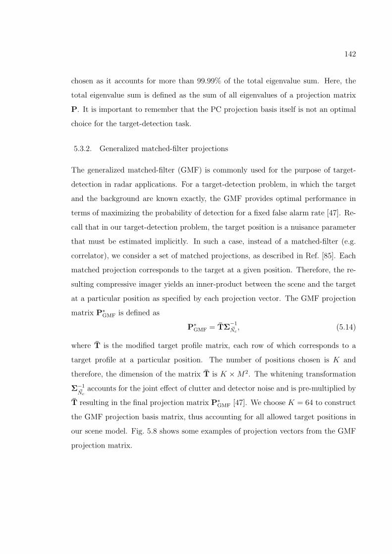
142
chosen as it accounts for more than 99.99% of the total eigenvalue sum. Here, the
total eigenvalue sum is defined as the sum of all eigenvalues of a projection matrix
P. It is important to remember that the PC projection basis itself is not an optimal
choice for the target-detection task.
5.3.2. Generalized matched-filter projections
The generalized matched-filter (GMF) is commonly used for the purpose of target-
detection in radar applications. For a target-detection problem, in which the target
and the background are known exactly, the GMF provides optimal performance in
terms of maximizing the probability of detection for a fixed false alarm rate [47]. Re-
call that in our target-detection problem, the target position is a nuisance parameter
that must be estimated implicitly. In such a case, instead of a matched-filter (e.g.
correlator), we consider a set of matched projections, as described in Ref. [85]. Each
matched projection corresponds to the target at a given position. Therefore, the re-
sulting compressive imager yields an inner-product between the scene and the target
at a particular position as specified by each projection vector. The GMF projection
matrix P∗GMF is defined as
P∗GMF = TΣ
−1~Nc, (5.14)
where T is the modified target profile matrix, each row of which corresponds to a
target profile at a particular position. The number of positions chosen is K and
therefore, the dimension of the matrix T is K ×M2. The whitening transformation
Σ−1~Nc
accounts for the joint effect of clutter and detector noise and is pre-multiplied by
T resulting in the final projection matrix P∗GMF [47]. We choose K = 64 to construct
the GMF projection basis matrix, thus accounting for all allowed target positions in
our scene model. Fig. 5.8 shows some examples of projection vectors from the GMF
projection matrix.
143
Figure 5.8. Example projection vectors in the GMF projection basis, clockwise fromupper left, #1,#16,#32,#64.

144
5.3.3. Generalized Fisher discriminant projections
The generalized Fisher discriminant (GFD) belongs to a class of linear discrimi-
nants that maximize the between-class separability while minimizing the within-class
variabilty [84]. For the target-detection task, this implies that the GFD projection
matrix is designed so that the conditional distributions under the “target-present”
and “target-absent” hypotheses are well-separated in the measurement space. Note
that the GFD projections achieve optimal discrimination when the conditional distri-
butions underlying each hypothesis are normally distributed with equal covariance.
However, for the target-detection task the conditional distributions underlying the
two hypotheses are not normally distributed and therefore, the GFD projection ma-
trix is not optimal. Nevertheless, we expect the GFD projections to improve upon
the GMF projections due to its compactness, which is critical in the presence of a
photon-count constraint. We consider two methods for designing the GFD matrix,
labeled as GFD1 and GFD2.
The GFD1 projection matrix is designed by considering each target position as
a separate hypothesis. Therefore, P target positions along with the target-absent
hypothesis result in a P + 1-class classification problem. The covariance under each
hypotheses is equal to the clutter covariance Σclutter and is defined as
Σi = Σclutter = c·HVcΣ~βVcT HT , i = 1 . . . P + 1. (5.15)
The mean under the ith “target-present” hypotheses (corresponding to a target-
present at the ith position) is given by
µi =√sH~Yi +
√cHVc~µ~β i = 1 . . . P, (5.16)
where ~Yi denotes the target profile at the ith position. The mean under the (P + 1)th
(i.e. null) hypothesis is
µP+1 =√cHVc~µ~β. (5.17)

145
Therefore, the overall mean is defined as
µGFD1 =1
2P
P∑
i=1
µi +1
2µP+1. (5.18)
Now, we can define the within-class scatter matrix SW1 and the between-class
scatter matrix SB1 required to compute the GFD1 projection matrix.
SW1 =1
2P
P∑
i=1
Σclutter +1
2ΣP+1 =
1
2
1
P+ 1
· Σclutter (5.19)
SB1 =1
2P
P∑
i=1
(µi − µGFD1)(µi − µGFD1)T
+1
2(µP+1 − µGFD1)(µP+1 − µGFD1)
T .
(5.20)
The GFD1 projection matrix P∗GFD1 maximizes the generalized Fisher discrimi-
nation criterion DGFD expressed as
DGFD(P∗GFD1) =
P∗TGFD1SB1P
∗GFD1
P∗TGFD1SW1P∗
GFD1
, s.t. P∗TGFD1SB1P
∗GFD1 = I. (5.21)
This is equivalent to solving the generalized eigenvalue problem, defined as
SB1P∗GFD1 = SW1Λ1P
∗GFD1. (5.22)
Note that the rank of P∗GFD1 is at most P . We retain the K dominant eigenvectors
of P∗GFD1 to construct the GFD1 projection matrix. For the work reported here we
retained K = 16 projection vectors in the GFD1 projection matrix, as they accounted
for 99.99% of the total eigenvalue sum. Fig. 5.9 shows some examples of projection
vectors from the GFD1 projection matrix.
To derive the GFD2 projection matrix, we consider an alternate two-hypothesis
problem which is somewhat more intuitive considering the target-detection task. The
means µ1 and µ2 under the “target-present” (variable target-position) hypothesis and
“target-absent” hypothesis respectively, are defined as
µ1 =1
P
P∑
i=1
√sH~Yi +
√cHVc~µ~β (5.23)

146
Figure 5.9. Example projection vectors in the GFD1 projection basis, clockwise fromupper left, #1,#10,#11,#14.

147
Figure 5.10. Projection vector in the GFD2 projection basis.
and,
µ2 =√cHVc~µ~β. (5.24)
Therefore, the overall mean is given by
µGFD2 =1
2µ1 +
1
2µ2 =
1
2P
P∑
i=1
√sH~Yi +
√cHVc~µ~β. (5.25)
The corresponding covariance matrices under the two hypothesis can be expressed
as
Σ1 =1
P
P∑
i
(√sH~Yi −
1
P
P∑
j
√sH~Yj)(
√sH~Yi −
1
P
P∑
j
√sH~Yj)
T
+ c · HVcΣ~βVcTHT
(5.26)
and
Σ2 = c · HVcΣ~βVcTHT . (5.27)
The within-class scatter matrix SW2 and between-class scatter matrix SB2 are
defined respectively as
SW2 =1
2Σ1 +
1
2Σ2 (5.28)
and,
SB2 =1
2· (µ1 − µGFD2)(µ1 − µGFD2)
T +
1
2· (µ2 − µGFD2)(µ2 − µGFD2)
T .(5.29)
148
As before, we find P∗GFD2 by solving SB2P
∗GFD2 = SW2Λ2P
∗GFD2. Note that the rank
of P∗GFD2 is now 1 as this is a two-class problem. Fig. 5.10 shows the single projection
vector that comprises the GFD2 projection matrix.
5.3.4. Independent component projections
Independent component (IC) analysis attempts to find a projection basis such that the
resulting projected data is statistically independent. Statistical independence implies
that the mutual-information between any pair of independent components is actually
zero. It is important to note that the pairwise mutual-information (among indepen-
dent components) is distinct from TSI, which is defined as the mutual-information be-
tween the virtual source variable and the measurements. In practice, an IC projection
basis is estimated from a training data set, similar to PC projections. Although an IC
algorithm attempts to achieve statistical independence, the resulting projection basis
may not actually achieve strict independence in practice. There are several methods
for performing IC analysis on a training data. For example, Bell’s infomax principle
of minimizing mutual-information between projected components [99], and the Fas-
tICA method that attempts to make the projected components as non-Gaussian as
possible [100] are two popular methods. We employ the FastICA approach in this
study due to its robustness and computational speed. For a comprehensive review of
the FastICA algorithm, we refer the reader to Ref. [100].
Before computing an IC projection matrix we apply the PC analysis as a pre-
processing step to whiten the training object data set. Recall that the dimensionality
of the original scene is M×M . As a result of selecting the first K dominant eigenvec-
tors from the PC projection matrix the dimensionality of the data set is reduced from
M2 to K. The FastICA algorithm is applied to this reduced-dimensionality training
data set to obtain a IC projection matrix of size K × K. In this work we begin
with a PC projection matrix using K = 32 in the pre-processing step to construct

149
Figure 5.11. Example projection vectors in the IC projection basis, clockwise fromupper left, #8,#16,#22,#28.

150
0 2 4 6 8 10 12 14 16 18 20 22 240
0.1
0.2
0.3
0.4
0.5
0.6
0.7
0.8
0.9
1.0
s
Tas
k−sp
ecifi
c In
form
atio
n [b
its]
GFD1
GMF
PC
IC
GFD2
Conventional
Figure 5.12. Optimized compressive imagers: TSI versus SNR for candidate CI systemand conventional imager.
the IC projection matrix. Fig. 5.11 shows examples of projection vectors from the IC
projection matrix.
5.4. Results and Discussion
We apply the TSI-based optimization framework to maximize the task-specific per-
formance of candidate CI systems each of which uses one of the projection bases
discussed above. The optimization process results in an optimal photon-allocation
vector ~π for a given value of SNR. This photon-allocation vector characterizes the
optimized design of a CI system and is specific to the particular choice of projection
matrix. Fig. 5.12 shows a plot of TSI versus SNR for each optimized candidate CI
system. The performance of a conventional imager is also plotted in Fig. 5.12 to

151
1 2 3 4 5 6 7 8 9 10111213141516171819202122232425262728293031320
1
2
3
4
5
6
7
8
9
Projection vector #
Pho
ton
allo
catio
n
(a)
1 2 3 4 5 6 7 8 9 10111213141516171819202122232425262728293031320
1
2
3
4
5
6
7
Projection vector #
Pho
ton
allo
catio
n
(b)
1 2 3 4 5 6 7 8 9 10111213141516171819202122232425262728293031320
1
2
3
4
5
6
Projection vector #
Pho
ton
allo
catio
n
(c)
Figure 5.13. Optimal photon allocation vectors for PC compressive imager at: (a)s = 0.5 , (b) s = 5.0 , and (c) s = 20.0.

152
facilitate a direct comparison with the optimized CI system designs. There are two
general trends that are evident from this plot, 1) TSI increases monotonically with
SNR, approaching the upper-bound of 1.0 bit asymptotically and 2) all CI system
designs outperform the conventional imager, with the exception of the GFD2 imager
which shows inferior performance at high SNR.
To understand the various mechanisms underlying the performance of a partic-
ular CI system design, let us begin by examining the PC imager design. Fig. 5.7
includes a plot of TSI versus SNR for the optimized PC imager design. It is ap-
parent from this plot that the optimized photon-allocation design outperforms the
uniform photon-allocation design of the PC imager. For example, at s = 5.0 the
non-optimized design achieves its maximum TSI of 0.38 bits at K = 16, while the
optimized design yields a higher TSI of 0.9291 bits. One reason for this improved
performance is that the optimized PC imager design avoids the rollover effect which
is present in the non-optimized design. This can be understood by considering that
the optimization process has two effects on the final imager design: 1) selection of
only those projection vector(s) that are most relevant to the task and 2) allocation
of the available photon-budget to the chosen projection vectors according to their
relative importance to the task. It is also important to realize that the optimal
photon-allocation depends strongly on SNR. To illustrate this effect, let us examine
the photon-allocation vector of the optimized PC imager design at three representa-
tive values of SNR as shown in Fig. 5.13. At a low SNR value of s = 0.5, we observe
that the optimal photon-allocation vector contains only 15 non-zero elements out of
a total of 32 possible. As SNR is increased to s = 5.0, the number of non-zero ele-
ments increases to 18, eventually reaching 19 for a high SNR value of s = 20.0. To
understand this SNR-dependent behavior, recall that these results are obtained using
a total photon-count constraint as defined in Eq. (5.12). This means that measuring
more features can only come at the expense of measuring fewer photons per feature.
Therefore, it is reasonable to expect that at low SNR (i.e., large AWGN variance), an

153
optimal photon-allocation strategy would result in selection of a minimum number of
projection vectors. This in turn maximizes the measurement fidelity along with dis-
tributing the photon-budget among the K most task-relevant projection vectors. As
SNR increases, we expect that the optimal ~π will employ non-zero photon-allocation
for relatively more projection vectors and result in higher TSI. This expectation is
in agreement with our observations from Fig. 5.13. We expect to observe similar
behavior in other candidate CI imager designs as well. Another interesting observa-
tion regarding the PC imager is that the distribution of photons as specified by its
optimal ~π, departs significantly from the eigenvalue distribution of the PC projection
basis. This is not surprising because the eigenvalue-based photon distribution is more
natural for a reconstruction-task instead of a detection-task.
Unlike the PC projection basis, the IC projection basis is not energy compact.
However, the IC projection basis has the inherent statistical independence property
that directly translates into a potential increase in TSI. To understand this, let us con-
sider two IC projection vectors, denoted by ~P1 and ~P2, that produce a measurement
R = [R1 R2]. The TSI in this measurement can be expressed as
I(R1, R2;X) = J(R1, R2) − J(R1, R2|X) (5.30)
= J(R1) + J(R2|R1) − J(R1, R2|X)
≤ J(R1) + J(R2) − J(R1, R2|X). (5.31)
Note that it is only when R1 and R2 are statistically independent that the equality
is achieved in Eq. (5.31), which is indeed the case for the IC projection basis. This
property of the IC projection basis has a direct impact on the number of projection
vectors that receive a non-zero photon-allocation when optimized. To illustrate this
effect, consider a noise-free scenario for which the IC imager requires Q projection
vectors to obtain a certain value of TSI, while the PC imager will require more than
Q projections to achieve the same TSI, due to the statistical dependence among its
basis vectors. In the presence of noise, the IC imager design would yield a higher TSI

154
as it utilizes fewer projection vectors and as a result achieves higher measurement
fidelity compared to the PC imager design. Therefore, it is reasonable to expect
that the optimized IC imager design would yield superior performance relative to the
optimized PC imager design. This is indeed the case. We observe that the optimized
IC imager design outperforms the optimized PC imager design in the low-to-mid SNR
region as shown in Fig. 5.12. For example, at s = 0.5 the IC imager achieves a TSI
of 0.3556 bits compared to 0.3012 bits for the PC imager. In the high SNR region,
the performance of the optimized IC and PC imagers becomes comparable as the
advantage of IC projections is diminished due to high measurement fidelity.
As discussed earlier, the “noise cost” effect arises from the total photon-count
constraint because of decreasing measurement fidelity with increasing K. It is due to a
higher noise cost incurred by the optimized GMF imager design that it does not exceed
the performance of the optimized PC and IC imager designs. Although, the GMF
projection matrix is optimal for extracting detection information from a given target
position, it requires all 64 projection vectors to achieve adequate performance over
the whole scene. However, the PC and IC projection bases require fewer projections
due to their energy compaction/statistical independence property and therefore, incur
a smaller noise cost. Thus, the optimality of the GMF projections (i.e. for a given
target position) is effectively countered by the smaller noise cost of the PC and IC
projections. From Fig. 5.12 we see that this results in slightly inferior TSI performance
for the GMF projections.
Among all the candidate compressive imagers considered in this study, it is clear
from Fig. 5.12 that the optimized GFD1 imager design yields the maximum task-
specific performance. For example, at s = 0.5 the GFD1 imager achieves a TSI
of 0.6017 bits compared to 0.2176 bits for GMF, 0.3012 bits for PC, 0.3556 bits for
IC and 0.1026 bits for the GFD2 designs. Similarly, at medium (s = 5.0) and high
(s = 20.0) SNR values, the GFD1 imager outperforms all other compressive imager
designs. The comparative performance of all the candidate imagers is quantified by

155
Imager/TSI@ s = 0.5 s = 5.0 s = 20.0
GFD1 0.6017 0.9841 0.9999
IC 0.3556 0.9324 0.9956PC 0.3012 0.9291 0.9944
GMF 0.2176 0.8461 0.9904GFD2 0.1026 0.4434 0.5922
Conventional 0.0051 0.0979 0.5568
Table 5.1. TSI (in bits) for candidate compressive imagers at three representativevalues of SNR: low(s = 0.5), medium(s = 5.0), and high(s = 20.0).
the data presented in Table 5.1 at three representative values of SNR. The supe-
rior performance of the GFD1 imager is primarily due to its projection basis design.
Recall that the GFD1 projection basis is derived to maximize the ratio of between-
class distance to within-class distance. This objective is equivalent to maximizing
the Kullback-Leibler distance (closely related to Shannon information) between the
two class-conditional distributions when they are normally distributed with equal co-
variances. For the target-detection task the two class-conditional distributions are
not Gaussian distributed and as a result, the discrimination information lies along
multiple dimensions. Although, the GFD1 projections does not achieve optimality
it does extract discriminating information along all available dimensions in an effi-
cient manner (i.e. with fewer projection vectors) which is the key to its enhanced
performance.
To gain further insight into the GFD1 imager design, let us examine its optimal
photon-allocation vector. It is interesting to note that at a low SNR of s = 0.5, the op-
timal photon-allocation vector has only 2 non-zero elements as shown in Fig. 5.14(a).
Comparing this to the 15 non-zero elements for the PC imager at the same SNR,
we can conclude that the discriminating information in the GFD1 projection basis
is represented more compactly than it is in the PC projection basis. As a result,
the noise cost in the case of the GFD1 imager is lower, thus yielding a larger TSI.

156
1 2 3 4 5 6 7 8 9 10 11 12 13 14 15 160
1
2
3
4
5
6
Projection vector #
Pho
ton
allo
catio
n
(a)
1 2 3 4 5 6 7 8 9 10 11 12 13 14 15 160
0.5
1
1.5
2
2.5
3
3.5
4
4.5
5
5.5
Projection vector #
Pho
ton
allo
catio
n
(b)
1 2 3 4 5 6 7 8 9 10 11 12 13 14 15 160
0.5
1
1.5
2
2.5
3
3.5
4
4.5
5
Projection vector #
Pho
ton
allo
catio
n
(c)
Figure 5.14. Optimal photon allocation vectors for GFD1 compressive imager at: (a)s = 0.5 , (b) s = 5.0 , and (c) s = 20.0.

157
Similarly, at mid-SNR and high-SNR values of s = 5.0 and s = 20.0, the optimal
photon-allocation vector of the GFD1 imager requires only 4 and 8 non-zero elements
respectively, while the PC imager uses 18 and 19 components respectively.
Finally, we observe that the GFD2 compressive imager yields the lowest TSI
among all candidate compressive imager designs. Note that the GFD2 projection
matrix has only one projection vector and therefore requires, no photon allocation
optimization. For the target-detection task, the two-class definition inherent in the
GFD2 projection matrix seems like a natural choice. However, the linear transfor-
mation approach used in Section. 5.3.3 to derive the GFD2 projection matrix is not
optimal. Recall that, this approach is optimal only when the underlying class con-
ditional distributions are Gaussian with equal covariance, which is certainly not the
case here. Also we noted earlier in this section that the discriminating information
does not lie along only one-dimension, but rather lies along multiple dimensions.
Therefore, the GFD2 projection matrix, being limited to only one projection vector,
results in inferior TSI performance compared to the other bases considered here.
5.5. Conventional metric: Probability of error
Recall that the performance of any algorithm designed to accomplish a specific task
is upper bounded by TSI [85]. This implies that for the target-detection task, TSI
provides an upper-bound on the performance of any detection algorithm. Tradition-
ally, a statistical measure such as the probability of error is employed in order to
quantify the performance of an imaging system for such a task. In this section, we
examine the relation between the TSI metric and the probability of error, to gain a
more traditional statistical perspective on the TSI-based design/analysis approach.
Fano’s inequality [67] provides the required relation between information-theory
and the probability of error for classification/detection tasks. It states that
J(X|R) ≤ Pe log(|X| − 1) + J(Pe), (5.32)

158
0 0.1 0.2 0.3 0.4 0.5 0.6 0.7 0.8 0.9 1.010
−4
10−3
10−2
10−1
100
Task−specific information [bits]
Pro
babi
lity
of e
rror
Figure 5.15. Lower bound on probability of error as a function of TSI.
where Pe is defined as the probability of error in detecting X conditioned on R, J(Pe)
denotes the entropy of Pe, and |X| represents the cardinality of X. Rewriting the
left-hand-side of Eq. (5.32) in terms of the mutual-information between X and R and
rearranging we obtain a direct relation between TSI and Pe
TSI ≡ I(X;R) ≥ J(X) − Pe log(|X| − 1) − J(Pe). (5.33)
For the target-detection task |X| = 2, substituting this into Eq. (5.33) we obtain,
TSI ≥ J(X) − J(Pe) = 1 + Pe log(Pe) + (1 − Pe) log(1 − Pe). (5.34)
Using this version of Fano’s relation, we can compute a lower bound on Pe as a
function of TSI.
Fig. 5.15 plots the lower bound on Pe from Eq. (5.34) as a function of TSI. Note
that this lower bound on Pe may not always be achievable. Nevertheless, the lower

159
0 2 4 6 8 10 12 14 16 18 20 22 2410
−8
10−7
10−6
10−5
10−4
10−3
10−2
10−1
s
Pro
babi
lity
of e
rror
Lower bound
Bayes’ detector
Figure 5.16. Comparison of probability of error obtained via Bayes’ detector versuslower bound obtained by Fano’s inequality as a function of SNR.
bound can still serve a useful purpose in comparing candidate imaging systems to
quantify their respective task-specific performance. To examine the tightness of this
lower bound we use the Bayes’ detector to obtain an estimate of the Pe that is
achievable in practice. The Bayes’ detector is defined using the maximum a-posteriori
(MAP) rule that is expressed as follows
pr(R|X = 0)
pr(R|X = 1)
X=1≶
X=0
pr(X = 1)
pr(X = 0), (5.35)
where pr(R|X = 1) and pr(R|X = 0) represent the conditional probabilities, pr(X =
1) and pr(X = 0) are the prior probabilities for the target-present and target-absent
hypotheses respectively. Here, X is defined as the output of the Bayes’ detector. The
inequality sign in Eq.(5.35) translates to the following decision rule: decide X = 1
if the right hand side is larger, otherwise decide X = 0. We will use the GFD1

160
imager as an example to investigate the relation between TSI and the Bayes’ bound
on Pe. The Bayes’ detector performance is simulated for a range of SNR values and
the resulting Pe is plotted as a function of SNR in Fig. 5.16 as the dashed curve.
The lower bound on Pe resulting from Fano’s relation in Eq. (5.34) is plotted as the
solid curve in Fig. 5.16. In the low SNR region, Pe achieved by the Bayes’ detector
is close to the lower bound derived from Fano’s inequality. For example, at s = 0.5,
the actual Pe achieved is 0.1099 compared to a lower bound of 0.0789. In general, we
observe that with increasing SNR the Bayes’ detector’s Pe follows the lower bound
closely.
5.6. Conclusions
A TSI-based optimization framework for designing CI systems was presented. The
task of target-detection was used to study the effectiveness of the optimized com-
pressive imager designs. Several projection bases were used to demonstrate the ap-
plication of the optimization framework to the design of CI systems. These included
the PC, IC, GMF, and GFD projection bases which were computed specifically for
the target-detection task. It was found that the optimized GFD1 compressive imager
outperformed all other compressive imagers because its projection matrix represented
the target-discrimination information most compactly. The GFD1 compressive im-
ager achieved a TSI of 0.6017 bits at s = 0.5, which is nearly three times that of the
GMF compressive imager. The relation between the information-theoretic TSI metric
and conventional probability of error (Pe) was also discussed. It was shown that the
TSI can be used to derive a lower bound on Pe for the task of target-detection. This
lower bound was compared to the actual Pe obtained using the Bayes’ detector for a
GFD1 compressive imager. It was demonstrated that the TSI metric correlates well
with conventional metrics such as Pe and may serve as a robust and tractable metric
for designing compressive imagers.

161
It is also important to consider the impact of various imperfections associated with
an actual implementation of a compressive imager design on its performance. For in-
stance, the SLM component used for implementing the projection vector has several
non-ideal characteristics such as less than 100% fill factor for each pixel, non-linear
pixel response with input voltage, limited gray-level resolution, non-uniform spatial
response, and noise in each pixel. The non-100% fill factor of pixels effectively reduces
the SLM transmission efficiency and therefore, it decreases the magnitude of the ac-
tual feature measurement on the detector resulting in a lower measurement SNR.
Similarly, the SLM pixel noise also reduces the feature measurement SNR. These two
effects lower the TSI of the compressive imager compared to the value predicted by
the simulation. In order to provide an example of this performance degradation, let
us assume a fill factor of 90% and a noise variance in SLM signal equivalent to 5%
of the detector noise variance. These two effects combine to reduce the measurement
SNR by nearly 15%, which in turn reduces the performance of the GFD1 compressive
imager from 0.9907 bits at s = 6 to 0.9841 bits that corresponds to s = 5. Further,
the non-linear pixel response, limited gray-level resolution, and the non-uniform spa-
tial response of the SLM also contribute to feature measurement errors that impact
the system performance negatively. Another practical issue related to CI system im-
plementation is use of negative elements in the projection vectors. To implement
projection vectors with both positive and negative values, a dual-rail approach can
be used, as described in Ref. [6]. The dual-rail approach has an associated noise cost
because the number of detectors is doubled [6]. We also note that the projection
vectors and their corresponding optimal photon-allocation vector changes with SNR,
this implies that we need to use different SLM masks and different exposure times for
low SNR conditions as opposed to a high SNR case. The projection vectors required
for a particular SNR can be realized by use of programmable SLMs and the desired
exposure time can be achieved by the use of variable apertures on each lenslet in
the parallel architecture. Although, the practical issues associated with compressive

162
imager implementation degrade the system performance it is important to emphasize
that the optimized CI designs still offer a significant performance improvement over
a conventional imager, especially at low SNR values.

163
Chapter 6
Conclusions and Future Work
We asserted in Chapter 1 that a joint-optimization of the optical and the post-
processing degrees of freedom provides a design framework that maximizes the per-
formance of a computational imaging system while utilizing all available (especially
optical) design resources most efficiently. Moreover, a task-specific approach within
the joint-optimization design framework allows the designer to leverage the available
degrees of freedom to maximize the imaging system performance for a specific task.
To evaluate the task-specfic approach, we considered an imaging system design study
for two separate tasks: object reconstruction and iris-recognition in Chapter 2 and
Chapter 3 respectively. Each task was considered in the context of imaging systems
whose detector array produce under-sampled measurements. In both of the design
studies the optical PSF, representing the optical degrees of freedom, was engineered
in conjunction with the post-processing algorithm parameters with the goal of over-
coming the performance degradations introduced by the detector under-sampling. In
the case of the object reconstruction task, the optical PSF was engineered via the use
of a pseudo-random phase-mask for two different metrics: resolution and reconstruc-
tion RMSE. It was observed that maximizing the resolution of the imaging system
resulted in a more diffused optical PSF compared to the optical PSF corresponding
to the optimal solution that minimized the reconstruction RMSE. The fact that the
optimal solutions were different for each of the two design metrics highlights the im-
portance of the design metric choice on the optimal imaging system design. Overall,
the optimized imaging systems achieved as much as 50% improvement in resolution
and nearly 20% lower reconstruction RMSE compared to the conventional imaging

164
system design that did not use an engineered optical PSF. For the iris-recognition
task, the optical PSF was engineered using a phase-mask that was represented by
Zernike polynomials. The optical PSF was jointly optimized with selected parame-
ters of the post-processing algorithm to maximize the imaging system performance
for the iris-classification task. In this case, the design metric used FRR and FAR
statistics to quantify the iris-recognition performance. The optimized imaging sys-
tem with the engineered optical PSF achieved a 33% performance improvement over
the conventional imaging system.
In general, the performance improvements obtained by the optimized imaging
systems for both the object reconstruction and the iris-recognition tasks demonstrate
the power of the optical PSF engineering method within the joint-optimization de-
sign framework. Note that the implementation of the optical PSF engineering method
considered here required a parametric representation of a phase-mask that is specified
by a finite set of parameters. As mentioned earlier, the phase-mask parameters repre-
sent the optical degrees of freedom of the imaging system considered in the two design
studies. While increasing the number of parameters of the phase-mask function in-
creases the volume of the optical design sub-space it also increases the computational
burden associated with the optimization process. On the other extreme, too few
phase-mask parameters artificially constrain the optical design sub-space potentially
excluding optimal solution(s). The choice of a particular phase-mask parametrization
therefore remains a challenging problem that requires further work to better under-
stand the trade-offs between the system performance, optimization complexity, and
from a practical point of view, the manufacturability of the optimized phase-masks
that is possible with the current machining/replicating technologies.
As note earlier, the optimal imaging system design is dependent on the particular
task, as quantified by the design metric (e.g. resolution vs. RMSE). This emphasizes
the concept of task-specific design and more importantly the crucial role of task-
specific design metrics within the joint-optimization design framework. In Chapter

165
4, the notion of task-specific information (TSI) was introduced as an information-
theoretic measure of an imaging system’s performance on a particular task. Various
source models were employed to demonstrate the utility of the TSI metric in quanti-
fying an imaging system’s performance for detection, classification, and localization
tasks. The role of the TSI metric in upper bounding the performance of an imaging
system design for a given task, irrespective of the post-processing algorithm, was also
discussed. Note that the source models employed for the TSI analysis were relatively
simple because their purpose was to simply demonstrate the application of TSI to
various tasks and different imaging system architectures. As discussed in Chapter 4,
the typical scenes encounter in reality require more sophisticated scene models (that
account for occlusion, shadow, perspective) to yield a realistic task-specific evaluation
of an imaging system. Therefore, more work needs to be conducted in formulating
realistic scene models along with the associated analysis that would be required for
computing the TSI. Another important aspect of the TSI analysis is the noise model,
we assumed it to be additive Gaussian noise. This noise model, in addition to ac-
counting for the detector read noise present in sensors also provides a relatively good
approximation to the shot-noise associated with detecting an optical signal under
bright-light conditions. However, under low-light conditions it becomes important to
take into account the actual Poisson distribution of the shot-noise. Therefore, our
imaging system model needs to be extended to include shot-noise and other sources
of noise that are encountered in an actual implementation of an imaging system. This
represents another direction for future work in extending the TSI analysis to more
realistic imaging systems. The application of TSI metric for engineering the optical
PSF to extend the depth of field of an imager was also considered within the context of
a texture classification task. A cubic phase-mask representation was used to optimize
the optical PSF to achieve a specified depth of field extension. The main goal of this
brief study was to demonstrate the application of TSI as a design metric to engineer
the optical PSF so as to achieve a desired imager performance for a particular task.

166
This study forms the basis for future work that would address the application of the
TSI metric for optimizing the optical PSF to accomplish more complex tasks such as
joint target detection and tracking.
Chapter 5 considered the extension of the TSI analysis framework developed in
Chapter 4 to the actual design of compressive imaging systems. The TSI design
framework was applied to design of compressive imaging systems for the task of
target detection. Several projections such as matched filter, generalized Fisher dis-
criminant, independent component analysis, and principal component analysis were
considered. The photon-allocation vector, representing the photon distribution to
each projection vector, was optimized using the TSI design metric for each candidate
compressive imaging system and the resulting optimized design solutions were eval-
uated and compared. Relative to a conventional imaging system the optimized com-
pressive system designs offered as much as six fold improvement in target-detection
performance at low SNR and nearly a two fold increase at higher SNR. The TSI
metric was also used to compute an upper-bound on the probability of detection for
GFD1 CI system design and was compared to the actual probability of detection from
the optimal Baye’s MAP detector. It was found that that upper-bound followed the
detector performance very closely over a range of SNR. In addition to the theoretical
results, we also discussed the various issues related with implementing a compres-
sive imaging system design in a physical system. In order to quantify the effect of
the various imperfections encountered in actual implementation of CI system further
analysis is required.

167
Appendix A: Conditional mean estimators for detection,
classification, and localization tasks
Here we derive explicit expressions for the conditional mean estimators E(~Y |~R) and
E(~Y |~R, ~X) for each of the three tasks: detection, classification, and localization.
E(~Y |~R) is defined as the expected value of ~Y given the measurement ~R and can
be written as
E(~Y |~R) =∑
l
~Yl Pr(~Y = ~Yl|~R) =∑
l
~Ylpr(~R|~Y = ~Yl) Pr(~Y = ~Yl)∑
m pr(~R|~Y = ~Ym) Pr(~Y = ~Ym)
, (A1)
where ~Yl spans over all the possible scenes that can be generated by the random
encoding function. Recall that for the detection task defined in Subsection 4.2.2,
~Y = T~ρX and virtual source X is binary. Therefore, for X = 1, ~Y can take P
different values corresponding to the P possible positions. ~Y is equal to zero for
X = 0. We define Pr(X = 1) = p, Pr(X = 0) = 1 − p, Pr(~Y = ~0) = 1 − p, and
Pr(~Y = ~Yl) = pP
, where l = 1, 2, .., P. Substituting these probabilities into (A1) we
obtain
E(~Y |~R) =
∑Pl=1 p
~Ylpr(~R|~Y = Yl)∑Pm=1 p[pr(
~R|~Y = Ym)] + (1 − p)P [pr(~R|~Y = 0)]. (A2)
Here the conditional probability density function pr(~R|~Y = ~Yl) is Gaussian and is
given by
pr(~R|~Y = ~Yl) =1
(2π)K/2√
detΣ~R|~Y
exp
[−1
2(Θ1 + Θ2l + Θ3l + Θ4)
](A3)
where Σ~R|~Y = c · PHVcΣ~β(PHVc)T + σ2
NI, (A4)
Θ1 = ~RTΣ−1~R|~Y
~R− 2√c · ~RT Σ−1
~R|~Y PHVc~µ~β, (A5)
Θ2l = −2√s · ~RTΣ−1
~R|~Y PH~Yl, (A6)
Θ3l = s · ~Y Tl HTPTΣ
−1~R|~Y PH~Yl + 2
√s · c · ~Y T
l HTPTΣ−1~R|~Y PHVc~µ~β, (A7)

168
and Θ4 = c · ~µT~βVT
cHTPTΣ−1
~R|~Y PHVc~µ~β. (A8)
Substituting (A3) into (A2) and simplifying yields the following expression
E(~Y |~R) =
∑Pl=1 p
~Yl · exp[−12(Θ2l + Θ3l)]∑P
m=1 p exp[−12(Θ2m + Θ3m)] + (1 − p)P
. (A9)
Note that here P represents the projection matrix of the projective imager and must
be assumed as I otherwise.
Next, consider the classification task specified in Subsection 4.2.3, where ~Y =
T~ρ ~X and virtual source ~X is binary. For ~X equal to [1, 0]T/[0, 1]T , ~Y will have P
possible values corresponding to as many positions. Assuming Pr( ~X = [1, 0]T ) = p,
Pr( ~X = [0, 1]T ) = 1 − p and equi-probable positions for both targets we obtain
E(~Y |~R) = (A10)∑P
l=1; ~X=[1,0]T p~Yl · exp[−1
2(Θ2l + Θ3l)] +
∑Pl=1; ~X=[0,1]T (1 − p)~Yl · exp[−1
2(Θ2l + Θ3l)]
∑Pm=1; ~X=[1,0]T p exp[−1
2(Θ2m + Θ3m)] +
∑Pm=1; ~X=[0,1]T (1 − p) exp[−1
2(Θ2m + Θ3m)]
.
This expression is similar to (A9) except for about twice as many terms in numerator
and the denominator.
For the joint detection and localization task, the estimator E(~Y |~R) can be ob-
tained by minor modifications to (A9). Considering the probabilities specified in
Subsection 4.2.4, the modified expression can be found as
E(~Y |~R) =
∑Qi=1
∑Pi
l=1Pr(X=i)
Pi
~Yi,l · exp[−12(Θi,2l + Θi,3l)]
∑Qj=1
∑Pj
m=1Pr(X=j)
Pj· exp[−1
2(Θj,2m + Θj,3m)] + (1 − p)
, (A11)
where Yi,l is the target profile at lth position of region i. Θi,2l and Θi,3l are evaluated
using (A6) and (A7) respectively by substituting Yl with the corresponding Yi,l. Sim-
ilarly for the joint classification and localization task, the estimator E(~Y |~R) can be
written as
E(~Y |~R) =
∑Qi=1
∑Pi
l=1
∑~α=[1,0]T ,[0,1]T
Pr(X=i,~α)Pi
~Yi,l,~α · exp[−12(Θi,2l + Θi,3l)]
∑Qj=1
∑Pj
m=1
∑~α=[1,0]T ,[0,1]T
Pr(X=j,~α)Pj
· exp[−12(Θj,2m + Θj,3m)]
, (A12)

169
where Yi,l,~α is the target profile specified by ~α at lth position of region i. Θi,2l and
Θi,3l are evaluated using (A6) and (A7) respectively by substituting Yl with respective
Yi,l,~α.
Now we derive the expressions for the estimator E(~Y |~R, ~X) required in evaluating
Eq. (4.18) for each task. The estimator is defined as
E(~Y |~R, ~X) =∑
l
~Yl · Pr(~Y = ~Yl|~R, ~X). (A13)
We may express the conditional probability Pr(~Y = ~Yl|~R, ~X) using Bayes’ law as
follows
Pr(~Y = ~Yl|~R, ~X) =pr(~R, ~X|~Yl) Pr(~Y = ~Yl)
pr(~R, ~X)(A14)
=pr(~R|~Y = ~Yl, ~X) Pr( ~X|~Y = ~Yl) Pr(~Y = ~Yl)∑
m pr(~R|~Y = ~Ym, ~X) Pr( ~X|~Y = ~Ym) Pr(~Y = ~Ym)
.(A15)
For the detection task in Subsection 4.2.2, the virtual source variable X is binary;
therefore, substituting (A15) and (A3) into (A13) and simplifying we obtain the
following expressions for the estimator
E(~Y |~R,X = 1) =
∑Pl=1
~Yl · exp[−12(Θ2l + Θ3l)]∑P
m=1 exp[−12(Θ2m + Θ3m)]
, (A16)
E(~Y |~R,X = 0) = 0,
where ~Yl in (A16) is the target profile at the lth position. Θ2l and Θ3l in (A16)
are evaluated using (A6) and (A7) respectively. Similarly for the classification task
defined in Subsection 4.2.3, the estimator in (A13) can be written as
E(~Y |~R, ~X) =
∑Pl=1
~Yl · exp[−12(Θ2l + Θ3l)]∑P
m=1 exp[−12(Θ2m + Θ3m)]
, (A17)
where ~Yl in this case is the target profile specified by ~X at lth position.
Recall from Subsection 4.2.4 that for the joint detection and localization task, the
virtual source variable X ′ is (Q + 1)-ary. Note that X ′ = X, where X denotes the

170
region in which target is present when α = 1 and X ′ = 0 when α = 0. The estimator
in (A13) for this case is given by
E(~Y |~R,X = i, α = 1) =
∑Pi
l=1~Yi,l · exp[−1
2(Θi,2l + Θi,3l)]∑Pi
m=1 exp[−12(Θi,2m + Θi,3m)]
, (A18)
E(~Y |~R, α = 0) = 0,
where X = i implies that target is present in region i, ~Yi,l is the target profile at
the lth position of region i. Once again Θi,2l and Θi,3l are evaluated using (A6) and
(A7) respectively by substituting Yl with the appropriate Yi,l. In a similar manner the
estimator E(~Y |~R, ~X) for the joint classification and localization task can be expressed
as
E(~Y |~R,X = i, ~α) =
∑Pi
l=1~Yi,l,~α · exp[−1
2(Θi,2l + Θi,3l)]∑Pi
m=1 exp[−12(Θi,2m + Θi,3m)]
, (A19)
where Yi,l,~α, Θi,2l and Θi,3l have the same meaning as in (A12).
171
References
[1] N. J. Wade and S. Finger, “The eye as an optical instrument: from cameraobscura to Helmholtz’s perspective,” Perception 30(10), 1157-1177 (2001).
[2] W. Boyle and G. Smith, “Charge Coupled Semiconductor Devices,” Bell SystemTechnical Journal 49, 587 (1970).
[3] G. E. Moore, “Cramming more components onto integrated circuits,” Electron-ics Magazine 38(8), (1965).
[4] E. R. Dowski and W.T. Cathey, “Extended Depth of Field Through WavefrontCoding,” Applied Optics 34(11), 1859-1866 (1995).
[5] P. Potuluri, U. Gopinathan, J. R. Adleman, and D. J. Brady, “Lensless sensorsystem using a reference structure,” Optics Express 11, 965-974 (2003).
[6] M. A. Neifeld and P. Shankar, “Feature-Specific Imaging,” Applied Optics 42,3379-3389 (2003).
[7] http://www.cdm-optics.com
[8] H. H. Barrett, “Objective assessment of image quality: effects of quantum noiseand object variability,” J. Opt. Soc. Am. A 7, 1266-1278 (1990).
[9] H. H. Barrett, J. L. Denny, R. F. Wagner, and K. J. Myers, “Objective assess-ment of image quality. II. Fisher information, Fourier crosstalk, and figures ofmerit for task performance,” J. Opt. Soc. Am. A 12, 834-852 (1995).
[10] H. H. Barrett, C. K. Abbey, and E. Clarkson, “Objective assessment of imagequality. III. ROC metrics, ideal observers, and likelihood-generating functions,”J. Opt. Soc. Am. A 15, 1520-1535 (1998).
[11] L. Poletto and P. Nicolosi, “Enhancing the spatial resolution of a two-dimensional discrete array detector,” Optical Eng. 38, 1748-1757 (1999).
[12] A. Papoulis, “Generalized sampling expansion,” IEEE Trans. Circuit Sys-tems 24, 652-654 (1977).
[13] S. Borman, “Topics in Multiframe Superresolution Restoration,” Ph.D. disser-tation (University of Notre Dame, Notre Dame, 2004).
[14] S. Farsiu, D. Robinson, M. Elad, and P. Milanfar, “Fast and robust multi-framesuper-resolution,” IEEE Trans. Image Process. 13, 1327-1344 (2004).

172
[15] N. Galatsanos and R. Chin, “Digital restoration of multichannel images,” IEEETrans. on Acoustics, Speech, and Signal Process. 37, 415-421 (1989).
[16] S. P. Kim, N. K. Bose, and H. M. Valenzuela, “Recursive reconstruction ofhigh resolution image from noisy undersampled multiframes,” IEEE Trans. onAcoustics, Speech, and Signal Process. 38, 1013-1027 (1990).
[17] H. Ur and D. Gross, “Improved resolution from subpixel shifted pictures,” Com-puter Vision Graphics Image Processing: Graph. Models Image Process. 54,181-186 (1992).
[18] M. Elad and A. Feuer, “Restoration of a single superresolution image from sev-eral blurred, noisy and undersampled images,” IEEE Trans. in Image Process. 6,1646-1658 (1997).
[19] J. Tanida, T. Kumagai, K. Yamada, S. Miyatake, K. Ishida, T. Morimoto,N. Kondou, D. Miyazaki, and Y. Ichioka,“Thin Observation Module by BoundOptics (TOMBO): Concept and Experimental Verification,” Applied Optics 40,1806-1813 (2001).
[20] Y. Kitamura, R. Shogenji, K. Yamada, S. Miyatake, M. Miyamoto, T. Mori-moto, Y. Masaki, N. Kondou, D. Miyazaki, J. Tanida, and Y. Ichioka, “Re-construction of a High-Resolution Image on a Compound-Eye Image-CapturingSystem,” Applied Optics 43, 1719-1727 (2004).
[21] P. M. Shankar, W. C. Hasenplaugh, R. L. Morrison, R. A. Stack, and M. A.Neifeld, “Multiaperture imaging,” Applied Optics 45, 2871-2883 (2006).
[22] M. A. Neifeld and A. Ashok, “Imaging using alternate point spread functions:Lenslets with pseudo-random phase diversity,” in Proceedings of OSA TopicalMeeting: Computational Optical Sensing and Imaging(COSI), Charlotte, NC,June 6-8, paper CMB1 (2005).
[23] A. Ashok and M. A. Neifeld, “Engineering the point spread function for super-resolution from multiple low-resolution sub-pixel shifted frames,” in Proceedingsof OSA Annual Meeting, Tucson, AZ, Oct 16-20 (2005).
[24] Q. Tian and M. N. Huhns, “Algorithms for subpixel registration,” ComputerVision Graphics Image Processing 35, 220-233 (1986).
[25] S. Verdu, Multiuser detection, (Cambridge, University Press, 1998), Chap. 2.
[26] J. Solmon, Z. Zalevsky , D. Mendlovicm, “Geometric Superresolution by CodeDivision Multiplexing,” Applied Optics 44, 32-40 (2005).

173
[27] A. Ashok and M. A. Neifeld, “Information-based analysis of simple incoherentimaging systems,” Optics Express 11, 2153-2162 (2003).
[28] H. H. Barrett and K. J. Myers, Foundations of Image Science, (Wiley-Interscience, 2004).
[29] J.W. Goodman, Introduction to Fourier Optics, (MCGraw Hill, 1996), Chap.7.
[30] E. Y. Lam, “Noise in superresolution reconstruction ,” Optics Letter 28, 2234-2236 (2003).
[31] H.C. Andrews and B.R. Hunt, Digital Image Restoration, (Prentice-Hall, En-glewood Cliffs, N.J., 1977).
[32] D. J. Tolhurst, Y. Tadmor, and T. Chao, “Amplitude spectra of natural im-ages,” Ophthalm. Physiol. Opt. 12, 229-232 (1992).
[33] D. L. Ruderman, “Origins of scaling in natural images,” Vision Res. 37, 3385-3398 (1997).
[34] D. J. Field and N. Brady, “Visual sensitivity, blur and the sources of variabilityin the amplitude spectra of natural scenes,” Vision Res. 37, 3367-3383 (1997).
[35] J. Burg, “Maximum entropy spectral analysis,” Ph.D. dissertation (StanfordUniversity, 1975).
[36] M. Irani and S. Peleg, “Improving resolution by image registration,” CVGIP:Graph. Models Image Process. 53, 231-239 (1991).
[37] A. P. Dempster, N. M. Laird and D. B. Rubin, “Maximum likelihood fromincomplete data via the EM algorithm,” J. Roy. Stat. Soc. Ser. B 39, 1-38(1977).
[38] L. B. Lucy, “An iterative technique for the rectification of observed distribu-tion,” Astron. J. 79, 745-754 (1974).
[39] W. H. Richardson, “Bayesian-based iterative method of image restoration,” J.Opt. Soc. Am. A 56, 1141-1142 (1972).
[40] A. Ashok and M. A. Neifeld, “ Recent progress on multidomain optimizationfor ultrathin cameras,” Proc. SPIE 6232, 62320N (2006).
[41] J. G. Daugman, “High confidence visual recognition of person by a test ofstatistical independence,” IEEE Trans. PAMI 15, 1148-1161 (1993).

174
[42] J. G. Daugman, “The importance of being random: statistical principles of irisrecognition,” Pattern Recognition 36, 279-291 (2003).
[43] J. G. Daugman, “How iris recognition works,” IEEE Trans. Circuits and Sys-tems for Video Tech. 14(1), 21-30 (2004).
[44] R. Barnard, V.P. Pauca, T.C. Torgersen, R.J. Plemmons, S. Prasad, J. van derGracht, J. Nagy, J. Chung, G. Behrmann, S. Mathews, and M. Mirotznik.“High-Resolution Iris Image Reconstruction from Low-Resolution Imagery,”Proc. SPIE 6313, 1-13, (2006).
[45] R. Narayanswamy, P. Silveira, H. Setty, V. Pauca, and J. van der Gracht, “Ex-tended depth-of-field iris recognition system for a workstation environment,”Proc. SPIE 5779, 41-50 (2005).
[46] R. Narayanswamy, G. E. Johnson, P. E. X. Silveira, and H. B. Wach, “Extendingthe imaging volume for biometric iris recognition,” Appl. Opt. 44, 701-712(2005).
[47] S. Kay, Fundamentals of Statistical signal processing: Detection theory, (Pren-tice Hall, 1993).
[48] CASIA-IrisV1 database, “http://www.cbsr.ia.ac.cn/IrisDatabase.htm”.
[49] M. Born and E. Wolf, Principles of Optics: Electromagnetic Theory of Prop-agation, Interference, and Diffraction of Light, (Pergamon Press, 1989) Chap.9.
[50] A. Papoulis and S. U. Pillai, Probability, Random Variables and StochasticProcesses, (McGraw Hill, 2001).
[51] C. L. Fales, F. O. Huck, and R. W. Samms, ”Imaging system design for improvedinformation capacity,” Applied Optics 23, 873-888, (1984).
[52] N. X. Nguyen, “Numerical Algorithms for Image Superresolution,” Ph. D. Dis-sertation, Stanford University, (2000).
[53] L. Masek, “Recognition of Human Iris Patterns for Biometric Identification,”Technical report, University of Western Australia, (2003).
[54] S. Sanderson and J. Erbetta, “Authentication for secure environments based oniris scanning technology,” IEE Colloquium on Visual Biometrics, (2000).
[55] D. J. Field, “Relations between the statistics of natural images and the responseproperties of cortical cells,” Journal of the Optical Society of America 4, 2379-2394 (1987).

175
[56] W. Wenzel and K. Hamacher, “A Stochastic tunneling approach for globalminimization,” Phys. Rev. Lett. 82(15), 3003-3007(1999).
[57] MPI 1.1 standard, http://www.mpi-forum.org/docs/mpi-11-html/mpi-report.html
[58] J. A. O’Sullivan, R. E. Blahut and D. L. Snyder,“Information-theoretic imageformation,” IEEE Trans. on Image Processing 44, 2094-2123 (1998).
[59] A. Ortega and K. Ramchandran, “Rate-distortion methods for image and videocompression,” IEEE Signal Processing Magazine 15, 23-50 (1998).
[60] F. O. Huck, C. L. Fales, and Z. Rahman, “An Information Theory of VisualCommunication,” Phil. Trans. R. Soc. A: Phys. Sci. and Engr. 354, 2193-2248(1996).
[61] F. O. Huck and C. L. Fales, “Information-theoretic assessment of sampled imag-ing systems,” Optical Engineering 38, 742-762 (1999).
[62] J. Ahlberg and I. Renhorn, “An information-theoretic approach to band selec-tion,” Proc. SPIE 5811, 15-23 (2005).
[63] S. P. Awate, T. Tasdizen, N. Foster, and R. T. Whitaker, “Adaptive, Nonpara-metric Markov Modeling for Unsupervised, MRI Brain-Tissue Classification,”Med. Image. Anal. (to be published).
[64] J. Liu and P. Moulin, “Information-Theoretic Analysis of Interscale and In-trascale Dependencies Between Image Wavelet Coefficients,” IEEE Trans. onImage Processing 10, 1647-1658 (2001).
[65] L. Zhen and Karam, “Mutual information-based analysis of JPEG2000 con-texts,” IEEE Trans. on Image Processing 14, 411-422 (2005).
[66] D. S. Taubman and M. W. Marcellin, JPEG2000: Image Compression Funda-mentals, Standards and Practice, (Springer Publishing, 2002)
[67] T. Cover and J. Thomas, Elements of Information Theory, (John Wiley andSons, New York, 1991).
[68] M. Tanner, Tools for Statistical Inference, (Springer, 2nd edition 1993).
[69] J. S. Liu, Monte Carlo Strategies in Scientific Computing, (Springer, 2001).
[70] C. P. Robert and G. Casella, Monte Carlo Statistical Methods, (Springer, 2004).
[71] A. Doucet, N. de Freitas, and N. Gordon, Sequential Monte Carlo Methods inPractice, (Springer, 2001).

176
[72] L. R. Bahl, J. Cocke, F. Jelinek, and J. Raviv, “Optimal decoding of linearcodes for minimizing symbol error rate,” IEEE Trans. Inform. Theory 20, 284-287 (1974).
[73] D. Guo, S. Shamai and S. Verdu, “Mutual information and minimum mean-square error in Gaussian channels,” IEEE Trans. on Inform. Theory 51, 1261-1282 (2005).
[74] H. L. Van Trees, Detection, Estimation, and Modulation Theory, Part I: De-tection, Estimation, and Linear Modulation Theory, New York: Wiley, 1968.
[75] D. P. Palomar and S. Verdu, “Gradient of mutual information in linear vectorGaussian channels,” IEEE Trans. on Inform. Theory 52, 141-154 (2006).
[76] W. T. Cathey and E. R. Dowski, “New Paradigm for Imaging Systems,” AppliedOptics 41, 6080-6092 (2002).
[77] A. Ashok and M. A. Neifeld, “Pseudorandom phase masks for superresolutionimaging from subpixel shifting,” Applied Optics 46, 2256-2268 (2007).
[78] M. D. Stenner, A. Ashok, and M. A. Neifeld, “Multi-Domain Optimization forUltra-Thin Cameras,” Frontiers in Optics, Rochester, NY (2006).
[79] “Multi-Domain Optimization,” http://ocpl.ece.arizona.edu/mdo/.
[80] M. A. Neifeld and J. Ke, “Optical architectures for compressive imaging,” Ap-plied Optics 46, 5293-5303 (2007).
[81] M. Turk and A. Pentland, “Eigenfaces for recognition,” Journal of CognitiveNeuroscience 3, 71-86 (1991).
[82] P. Belhumeur, J. Hespanha, and D. Kriegman, “Eigenfaces vs. Fisherfaces:Recognition Using Class Specific Linear Projection,” IEEE Trans. on Patternanalysis and Machine intelligence 19, 711-720 (1997).
[83] M. S. Bartlett, J. R. Movellan, T. J. Sejnowski, “Face recognition by inde-pendent component analysis,” IEEE Trans. on Neural Networks 13, 1450-1464(2002).
[84] R. O. Duda, P. E. Hart, and D. G. Stork, Pattern Classification, (Wiley Inter-science 2000).
[85] M. A. Neifeld, A. Ashok, and P. K. Baheti, “Task Specific Information forImaging System Analysis,” J. Opt. Soc. Am. A 24, B25-B41 (2007).

177
[86] H. Pal and M. A. Neifeld, “Multispectral principal component imaging,” OpticsExpress 11, 2118-2125 (2003).
[87] D. L. Donoho, “Compressed sensing,” IEEE Trans. on Information Theory 52,1289-1306 (2006).
[88] M. Lustig, D. L. Donoho, J. M. Santos, J. M. Pauly, “Compressed Sensing MRI[A look at how CS can improve on current imaging techniques],” IEEE SignalProcessing Magazine. 25, no. 2, 72-82, March 2008.
[89] A. Mahalanobis, “Optical Systems for Task Specific Compressed Sensing andImage Reconstruction,” Annual meeting of the IEEE Lasers and Electro-OpticsSociety, 157-158, Oct 2007.
[90] M. F. Duarte, M. A. Davenport, M. B. Wakin and R. G.Baraniuk,“Sparse signaldetection from incoherent projections,” in Proc. of IEEE International Conf.Acoustics, Speech and Signal Processing (ICASSP), vol. 3, 14-19 (2006).
[91] D. Takhar, J. N. Laska, M. B. Wakin, M. F. Duarte, D. Baron, S. Sarvotham,K. Kelly, and R. G. Baraniuk, “A new compressive imaging camera architectureusing optical-domain compression,” Proc. SPIE 6065, 43-52 (2006).
[92] D. P. Palomar and S. Verdu, “Representation of Mutual Information Via InputEstimates,” IEEE Trans. on Inform. Theory 53, 453-470 (2007).
[93] N. Towghi and B. Javidi, “Optimum receivers for pattern recognition in thepresence of Gaussian noise with unknown statistics,” J. Opt. Soc. Am. A 18,1844-1852 (2001).
[94] R. Patnaik and D. Casasent, “MINACE filter classification algorithms for ATRusing MSTAR data,” Proc. SPIE 5807, 100-111 (2005).
[95] R. Patnaik and D. Casasent, “SAR classification and confuser and clutter re-jection tests on MSTAR ten-class data using Minace filters,” Proc. SPIE 6574,657402:1-15 (2007).
[96] W. Gander and W. Gautschi, “Adaptive Quadrature - Revisited,” BIT 40,84-101 (2000).
[97] I. T. Jolliffe, Principal Component Analysis, (Springer, 2002).
[98] D. Barber and F. V. Agakov, “The IM Algorithm: A Variational Approach toInformation Maximization,” In NIPS (MIT Press, 2003).
[99] A. J. Bell and T. J. Sejnowski, “An information-maximization approach to blindseparation and blind deconvolution,” Neural Computation 7, 1129-1159 (1995).

178
[100] A. Hyvarinen, J. Karhunen, and E. Oja, Independent Component Analysis,(Wiley, 2001).
Related Documents