A Tale of Two Countries: Sovereign Default, Trade, and Terms of Trade Grace W. Gu * August 3, 2015 (click here for the latest version) Abstract Sovereign defaults are associated with income and trade reductions and terms- of-trade deterioration. This paper develops a two-country model to study the inter- actions between foreign-debt default risk, income, trade, and terms of trade. Debt crises are costly because they adversely affect the vertical integration of production between the creditor and the borrower. Consequently, trade flows change due to income losses and home bias in consumption. The defaulter’s terms of trade also deteriorate endogenously, which accelerates its income and trade losses. The model produces procyclical imports, exports, and terms of trade, and other empirical fea- tures of Mexicos business cycles and default episodes. Keywords: sovereign default, terms of trade, real exchange rate, trade, DSGE. JEL code: F34 - F41 - F44 * Gu: Department of Economics, UC Santa Cruz, Engineering 2 Building, Room 463, Santa Cruz, CA 95060, [email protected]. I thank Laura Alfaro, Yan Bai, Paul Bergin, George Bulman, Michael Dooley, Fabio Ghironi, Michael Hutchinson, Ken Kasa, Ken Kletzer, Huiyu Li, Eswar Prasad, Katheryn Russ, Ina Simonovska, Alan Spearot, Viktor Tsyrennikov, Carl Walsh, Beiling Yan, Vivian Yue, as well as many others, for their incredibly helpful discussions. This paper has also benefited from comments from conference/seminar participants at Cornell, AEA-Boston, UC Davis, UC Riverside, UC Santa Barbara, UC Santa Cruz, Santa Clara Univ, Atlanta Fed, Peking Univ, Tsinghua Univ, San Francisco Fed, and NBER Summer Institute.

Welcome message from author
This document is posted to help you gain knowledge. Please leave a comment to let me know what you think about it! Share it to your friends and learn new things together.
Transcript

A Tale of Two Countries:
Sovereign Default, Trade, and Terms of Trade
Grace W. Gu∗
August 3, 2015
(click here for the latest version)
Abstract
Sovereign defaults are associated with income and trade reductions and terms-
of-trade deterioration. This paper develops a two-country model to study the inter-
actions between foreign-debt default risk, income, trade, and terms of trade. Debt
crises are costly because they adversely affect the vertical integration of production
between the creditor and the borrower. Consequently, trade flows change due to
income losses and home bias in consumption. The defaulter’s terms of trade also
deteriorate endogenously, which accelerates its income and trade losses. The model
produces procyclical imports, exports, and terms of trade, and other empirical fea-
tures of Mexicos business cycles and default episodes.
Keywords: sovereign default, terms of trade, real exchange rate, trade, DSGE.
JEL code: F34 - F41 - F44
∗Gu: Department of Economics, UC Santa Cruz, Engineering 2 Building, Room 463, Santa Cruz, CA95060, [email protected]. I thank Laura Alfaro, Yan Bai, Paul Bergin, George Bulman, Michael Dooley,Fabio Ghironi, Michael Hutchinson, Ken Kasa, Ken Kletzer, Huiyu Li, Eswar Prasad, Katheryn Russ,Ina Simonovska, Alan Spearot, Viktor Tsyrennikov, Carl Walsh, Beiling Yan, Vivian Yue, as well asmany others, for their incredibly helpful discussions. This paper has also benefited from comments fromconference/seminar participants at Cornell, AEA-Boston, UC Davis, UC Riverside, UC Santa Barbara,UC Santa Cruz, Santa Clara Univ, Atlanta Fed, Peking Univ, Tsinghua Univ, San Francisco Fed, andNBER Summer Institute.
1 Introduction
Sovereign debt default events are associated with three empirical regularities: (a) deep
recessions, (b) a decline in international goods trade, and (c) deteriorating terms of trade
and real exchange rates. Recent evidence shows that, across countries, default episodes
have on average been accompanied by a GDP drop of 5 percent below trend, a bilateral
trade value decline of 8 percent, and real depreciation of 30-50 percent.1 However, these
three phenomena have not been addressed simultaneously by existing sovereign default
models. This paper fills the gap by studying how foreign-debt default risk and occurrences
endogenously interact with income, terms-of-trade, and international goods trade through
production vertical integration in a two-country DSGE model.2
The model features four key elements. First, the model has default risk and occur-
rences (as in Eaton and Gersovitz, 1981; Aguiar and Gopinath, 2006; Arellano, 2008; and
Mendoza and Yue, 2012). The second key element is consumption home bias in both
countries. In the model, I show that as the borrower country’s default risk increases
with debt, its budget constraint tightens and its terms of trade deteriorate due to home
bias and reduced world relative demand for its final good. Deterioration in the terms
of trade prevents the borrower country from real appreciation that could have eased the
debt burden denominated in the creditor country’s final good. Thus, the default risk
increases further. In this way, the default risk interacts with the terms of trade and the
real exchange rate prior to a sovereign default.
The third key element of the model is vertical integration of production, where some
firms in the creditor country import an intermediate good from the borrower country to
produce a final good.3 The last key element of the model is a default penalty through the
vertical integration. When a large adverse productivity shock causes the borrower country
to default, the event triggers an efficiency loss in the creditor-country firms’ operations
regarding the intermediate good input from the defaulting country, which causes the
demand for the intermediate good to decline.
Empirical analyses indicate such efficiency loss exists. Specifically, this paper finds
that Canadian output was negatively affected by Mexican default events and the size of
1See Rose (2005), Cuadra and Sapriza (2006), Reinhart and Rogoff (2011), and Mendoza and Yue(2012).
2As illustrated in the model and result sections of this paper, the two-country model differs from asmall open economy model in offering unique insights about bond market equilibrium pricing and theimpact of a sovereign default on a creditor country’s income.
3Here the vertical integration is narrowly defined. It does not include activities where creditor countryfirms export an intermediate good to borrower country. Mendoza and Yue (2012) use this latter channelfor a default penalty.
1

the impact increases with an industry’s dependency on Mexican inputs. Moreover, the
efficiency loss in vertical integration is also consistent with other papers’ empirical findings
that foreign firms’ activities (e.g., FDI, offshoring, and other global sourcing) are more
severely damaged than domestic firms’ in a crisis country, possibly due to crisis-elevated
trade costs, information asymmetry, and risk aversion (e.g., Brennan and Cao, 1997; Tille
and van Wincoop, 2008; Milesi-Ferretti and Tille, 2010; and Broner, Didier, Erce, and
Schmukler, 2013).4
The decline in foreign demand for the intermediate good upon default in the model
generates an income loss additional to that from the initial adverse productivity shock in
the defaulting country. Its wealth declines relative to the creditor country’s because its
overall income loss exceeds the gain from not repaying the debt. This reduces the world
relative demand of the defaulting country’s final good, due to home bias in consumption.
Therefore, its terms of trade and real exchange rate deteriorate, taking a third toll on
income and trade. In this way, the model builds an endogenous terms-of-trade mechanism
by which a sovereign default amplifies the effects of adverse productivity shocks on the
borrower country’s income and trade.5
This paper contributes to the literature by examining the role of vertical integration
for both creditor and borrower countries during sovereign debt crises. In particular, it in-
corporates the impact of sovereign default on creditor-country firms’ vertically integrated
production activities with the defaulting country. This produces a sovereign-default cost
to both the creditor and the borrower countries, which affects their debt contract.
The second contribution of this paper is that it studies the endogenous consequences
of a sovereign default to income, trade, terms of trade, and real exchange rate, and thus
how they affect the incentives to default. For one thing, the model captures reductions
in trade flows during default episodes, which have been well studied in the empirical
literature (e.g., Rose, 2005), but not in the theoretical literature. Modeling this stylized
fact helps us understand how a country’s consumer preferences regarding home goods and
imports affect its propensity to default (Rose and Spiegel, 2004; Rose, 2005).6
For another, this paper endogenizes terms of trade and real exchange rate in a sovereign
4Moreover, Fuentes and Saravia (2010) find that a default event can reduce FDI inflows by 72 percent.Aizenman and Marion (2004) also document that greater supply uncertainty reduces the expected incomefrom vertical FDI.
5It is worth emphasizing that, as in previous sovereign default models, this paper’s default also arisesin equilibrium as an optimal decision of a benevolent government.
6Past empirical research suggests that less outward-oriented sovereigns are more willing to default.Therefore, if a sovereign government internalizes its citizens’ desire for imported goods, we can begin toconsider how a country’s reduced desire for foreign goods can spur defaults, or how we can motivate thecountry to service its debt on time.
2

default model. It captures their two-way interaction with default risk prior to sovereign
default occurrences. During sovereign default events, it also captures the terms of trade
and real exchange rate deteriorations as they contribute to a defaulting country’s income
and trade losses. For instance, for 45 sovereign default episodes in 27 developing countries
over the period 1977-2009, on average at least half of the defaulting countries’ losses of
output and export value came from real depreciation.7 Therefore, the terms of trade and
real exchange rate in my model results in an endogenous penalty on income and trade
upon default. That is, unlike many previous sovereign default models, this model does
not rely on an exogenous endowment loss.8
In a quantitative exercise, I apply the model to the Mexican debt crises in the 1980s
and the country’s business cycles for the period of 1981Q1-2012Q4.9 This model generates
three empirical features of emerging markets’ business cycles and their sovereign default
episodes. First, it delivers countercyclical trade balances and procyclical trade flows.
Second, the model supports high bond spreads that are also countercyclical. Third, the
model accounts for terms-of-trade deterioration, real depreciation, and trade flow and
GDP declines during and right after a sovereign default.
To further study the role of terms of trade in affecting income, I examine the model
results where GDP and trade losses are partially due to terms-of-trade deterioration and
partially due to volume changes, as in the data. I also evaluate the welfare of both
countries, as the welfare of the creditor country is often left out of existing sovereign
default models. This reveals that upon default, both countries’ welfare declines, but
higher vertical integration and maintaining healthy foreign business environment reduce
their post-default welfare losses.
In explaining the cyclical movements of trade balances and terms of trade, this paper
is related to other studies in the international business cycle literature.10 But many of
them ruled out actual default events in equilibrium, unlike this model. Thus this paper is
closely related to sovereign debt literature (e.g., Grossman and Van Huyck, 1988; Kletzer
and Wright, 2000; Alfaro and Kanczuk, 2005), especially to previous quantitative small-
7The relevant figure is not included in this version of the paper due to space limitation, but is availableupon request. All data are real, logged, and HP-filtered. Raw data sources are detailed in the Appendix.
8It is similar to Mendoza and Yue (2012), where their model endogenizes output losses by a productionefficiency loss due to a default-triggered decline of trade credit to import inputs.
9I chose Mexico for this two-country model because Mexico has a relatively large open economy amongthe countries that have recently defaulted, as well as relatively large vertically integrated sectors involvedin foreign production, including its maquiladora sector (Zlate, 2012).
10These include but are not limited to works by Backus, Kehoe, and Kydland (1992, 1994), Mendoza(1995), Stockman and Tesar (1995), Heathcote and Perri (2002), Kehoe and Perri (2002), Kose (2002),Broda (2004), Iacoviello and Minetti (2006), Bodenstein (2008), and Raffo (2008).
3

open-economy sovereign default models, such as those by Aguiar and Gopinath (2006),
Arellano (2008), and Mendoza and Yue (2012), based on Eaton and Gersovitz (1981).
They have made significant contributions to endogenizing default risk (and income), as
well as to accounting for key empirical patterns of developing countries’ business cycles
and default episodes. However, those models do not focus on default-triggered changes
to trade flows and the terms of trade.
A few recent sovereign default papers (Cuadra and Sapriza, 2006; and Bleaney, 2008;
Popov and Wiczer, 2014) have examined the roles of exogenous terms-of-trade shocks and
exogenous terms-of-trade default penalty in small open economy models. The inclusion of
endogenous terms of trade and real exchange rate distinguishes this paper from them. Na,
Schomitt-Grohe, Uribe, and Yue (2014) also include endogenous exchange rate but focus
on optimal exchange rate policy. Like the model in this paper, their model achieves con-
current default and depreciation. However, their depreciation is driven by wage rigidity
and the government’s intention to reduce unemployment, whereas this model’s deprecia-
tion is associated with consumption home bias and changes to trade flows. Most recently,
Asonuma (2014) has also endogenized the real exchange rate in a two-country sovereign
default model, but through a different mechanism in endowment economies.11 In this
paper, I use production economies to incorporate richer business cycle fluctuations.
In addition, this paper complements the vast literature about international trade and
financial crises with incomplete markets, especially for emerging economies (e.g., Mendoza
2002, 2003, 2010). More specifically, it fits in the existing strand that focuses on the
connection between international trade and sovereign defaults, and the strand on the
connection between trade and exchange rate.
In the former strand, which consists largely of empirical studies, Rose (2005) docu-
ments that a default can reduce real bilateral trade value (in USD) by 8 percent for an
extended period after the event. However, it remains unclear why trade declines. The
four hypotheses – trade sanctions, trade credit collapse, asset seizures, and reputation –
are commonly mentioned, but the empirical evidence supporting them remains ambigu-
ous (Martinez and Sandleris, 2011; Tomz and Wright, 2013). One exceptional theoretical
model is proposed by Bulow and Rogoff (1989), who apply creditors’ seizures of a de-
faulting country’s exports. This paper instead incorporates vertical integration and terms
of trade to examine the interaction between trade and sovereign defaults. In the latter
strand of literature on trade and exchange rate, this paper is related to works by Bald-
win and Krugman (1989), Alessandria, Kaboski, and Midrigan (2010), Engel and Wang
11Asonuma (2014) uses traded and non-traded goods to generate real depreciation in his model, similarto the idea proposed by Arellano and Kocherlakota (2014).
4
(2011), Drozd and Nosal (2012), and Alessandria, Pratap, and Yue (2014). My model
differs by endogenizing default risk in interest rates.
The remainder of this paper is organized as follows. Section 2 describes the model
environment, equilibrium, and mechanisms. Section 3 provides the model calibration and
quantitative results. Section 4 concludes.
2 Model
2.1 Environment
In this section, I describe a dynamic model of two countries with endogenous sovereign
default, terms of trade, real exchange rate, and risk averse agents. In the model, the two
countries (i = 1, 2) trade one-period discount bonds, produce two unique final goods (j =
1, 2), respectively, and consume both through trade. The two final goods are imperfect
substitutes with constant elasticity, and cij stands for country i’s consumption of final
good j. pj stands for the final good j’s price, and country 1’s final good price p1 is
normalized to 1. I assume that the nominal exchange rate between the two countries is
1, and thus the real exchange rate is the ratio of country 2’s over country 1’s aggregate
price index. When the ratio decreases, country 2 experiences real depreciation.
I set country 1 to be the creditor who never defaults and has constant productivity
e1; country 2 is the borrower who has an option to default on its sovereign bonds and
faces stochastic productivity e2 that follows a Markov chain.12 Creditor country 1 has a
fixed amount of capital, k1, which can be paired either with a fixed amount of domestic
labor n1 to produce the final good 1, or with an imported intermediate good produced by
borrower country 2’s labor to produce the same final good 1. I use k1 to denote capital
used with domestic labor, km to denote that used with imported intermediate inputs, and
k1 + km = k1.13 Borrower country 2 has a fixed amount of labor, n2. It is divided into nm
who produce intermediate inputs for creditor country 1, and n2 = n2 − nm who produce
final good 2 with domestic capital k2.
12One way to interpret the creditor country’s constant productivity is that it always can smooth itsproduction through other financial channels that are not in this model, regardless of the situation in thebond market with the borrower country. Moreover, since the creditor country never defaults, it is not ofinterest in this paper to complicate the model results by including its productivity shocks. It would beof future research interest, however, to study the spillover effects when a creditor country’s productivityshocks trigger a borrower country’s sovereign default.
13Another setup is creditor country 1’s imported intermediate good and domestic labor directly sub-stitute each other imperfectly as inputs, and produce final good 1 with capital. Similar results areexpected, but it emphasizes the role of labor substitution in the creditor country, whereas the currentsetup emphasizes the role of capital allocation and has the flexibility to alternatively interpret km as FDI.
5

Three reasons stand out for this asymmetric model setup, where creditor country 1
allocates capital and borrower country 2 allocates labor and produces the intermediate
good for exporting. First, many of the countries that have recently defaulted are devel-
oping or emerging economies, where labor tends to be abundant and is used to produce
intermediate goods for export, through vertical FDI, offshoring, and other global sourcing
activities. Second, even though creditor country 1 does not produce intermediate goods,
its domestic labor input is an imperfect substitute for the imported intermediate good
and can be considered as creditor country 1’s own implicit intermediate inputs.
Third, the impact of a sovereign default on the demand for borrower country 2’s
intermediate good exports serves as one of the default penalties in the model. Even
though the data show defaulting countries’ intermediate good imports are also usually
damaged, I extract it from this paper because the inclusion makes it difficult to single
out the impact of the intermediate good export reduction upon default as a penalty,
which is the focus of this paper. The current setup keeps the model tractable, yet retains
a connection to reality. However, it is interesting to include more channels of global
integration in future research.14
It is also worth noting that borrower country 2 produces the intermediate good only
for export, not for domestic use. It is to distinguish the globally integrated production
activities from purely domestic activities in the borrower country. Because the two types
of activities are affected differently by crises, according to empirical studies mentioned in
the introduction. Meanwhile, we can consider those intermediate goods for domestic use
to be embedded in the value of borrower country 2’s final good 2.
In the bond market, a non-state-contingent one-period bond denominated in the cred-
itor country’s final good 1 is traded between the two countries. The bond is denoted
as bi for country i’s asset holdings. The borrower country’s default can be triggered by
negative productivity shocks and can happen along the equilibrium. The two countries
hold their own beliefs/concerns about borrower country 2’s default probabilities, while the
actual default probabilities are endogenous to debt holding and fundamental. Risk-averse
creditors in country 1 are willing to offer debt contracts that in some states may result in
a default by charging a high interest rate. Hence, equilibrium interest rates reflect the two
countries’ concerns about the default probabilities, as well as the creditor’s consumption
changes and risk aversion (Lizarazo, 2013).
The timing of this model is as follows. Both countries start off with initial sovereign
bond assets. After they observe the current productivity shock, borrower country 2 decides
14Mendoza and Yue (2012) use a default-triggered intermediate good import reduction as the defaultpenalty and reach a similar output-loss result as this paper does.
6

whether to repay its debt. If it does not default, bond market equilibrium determines the
bond price and the next period’s quantity. If it defaults, both countries enter financial
autarky and return with a certain probability, and creditor country 1 firms’ operations
with the intermediate good from borrower country 2 suffer from an efficiency loss. Then
accordingly, both countries reallocate their capital and labor. And last, production, trade,
and consumption take place. The following sections describe the model specifications.
2.2 Country 1: Creditor
Creditor country 1 has two types of agents: representative firms, and households.
2.2.1 Firms
Firms hire domestic workers n1, rent capital from households, choose capital allocation
{k1, km}, and decide how many intermediate good inputs to import from borrower coun-
try 2.15 Firms’ goal is to maximize their profits, taking wage w1, capital rent r1, and
intermediate good price pm as given:
Π1 = maxn1,qm,k1,km
{e1n
α11 k
1−α11 − w1n1 − r1k1 + e1(εqm)α3k1−α3
m − pmqm − r1km}
(1)
The first three terms are the profit the firms gain from using domestic labor n1 to
produce final good 1. The last three terms are the profit the firms gain from using
intermediate inputs εqm to produce final good 1, after deducting intermediate good costs
and capital rents. ε symbolizes the firms’ efficiency of operating with the intermediate
good from borrower country 2. When the borrower country is not in default, ε = 1. When
the borrower country is in default, a small portion of its intermediate good used by country
1’s firms is lost in operation. More specifically, during default episodes ε = min(ε e2e2, 1),
where 0 < ε < 1 and e2 is borrower country 2’s average productivity. This formulation
has four indications.
First, creditor country 1 firms’ production using the foreign intermediate good suffer
from an additional efficiency loss on top of the defaulting country’s negative aggregate
productivity shock that lowers its intermediate good production in the first place.16 This
15The model results would not be different if country 1’s firms internalize the production decision ofthe intermediate good sector in borrower country 2. The arrangement would be similar to that used inthe global sourcing literature (Antras and Helpman, 2004). But the current setup helps the model clarifythat the default-triggered efficiency loss is on the creditor country firms’ operations, not directly on thedefaulting country firms and their intermediate good production and exports.
16Unless the aggregate productivity in defaulting country 2 is already lower than εe2. The modelcalibration ensures that min(e2) > εe2.
7

setup reflects the empirical findings that foreign firms’ activities (e.g., FDI, offshoring,
and other global sourcing) are more severely damaged than domestic firms’ activities
in a crisis country, as evidenced by but not limited to Brennan and Cao (1997), Tille
and van Wincoop (2008), Milesi-Ferretti and Tille (2010), and Broner, Didier, Erce, and
Schmukler (2013).
Second, the default-triggered efficiency loss lies only in the foreign operations of country
1’s firms, not in defaulting country 2’s firms, given that the latter are already subject
to the negative aggregate productivity shocks that trigger sovereign defaults. Hence, the
model assumes that default events and efficiency losses in ε do not directly affect the
supply of the intermediate good. It is country 1 firms’ demand of the intermediate good
that is directly affected, possibly due to defaulting country 2’s worsened foreign business
environment and/or crisis-elevated trade costs and information asymmetry that cause
country 1 firms’ marginal cost of operating with the imported intermediate good to rise.
Third, the efficiency loss is applied only to country 1 firms’ production using im-
ported inputs from the defaulting country, not to their production using domestic inputs,
for which this paper provides empirical support. In the regression analysis, Mexico is
used for the defaulting country and Canada for the creditor country, as in the model
calibration. I collect Canadian monthly output data on 13 manufacturing industries for
the period from January 1981 to October 2012. After controlling for crisis-impacts from
the U.S., Canadian business cycles, and industry-specific trends and other factors, I find
negative impacts of Mexican sovereign default episodes on Canadian manufacturing out-
puts. Moreover, a Canadian industry that uses more Mexican inputs is more negatively
affected by those default episodes than an industry that uses less Mexican inputs. See
the Appendix for more details.
Last, the formulation of ε generates efficiency losses and default penalties that increase
with defaulting country 2’s productivity state, such that, all else being equal, the borrower
country has a larger incentive to default at a lower productivity state. This is consistent
with previous sovereign default models (Arellano, 2008).
2.2.2 Households
Households in creditor country 1 supply fixed amounts of capital k1 and labor n1 to the
firms. They use the proceeds from firms for consumption to maximize a standard time-
separable utility function E[∑∞
t=0 βt1U(c11t, c12t)], where 0 < β1 < 1 is the discount factor
and U(.) is a one-period utility function that is continuous, homothetic, strictly increasing
and concave, and satisfies the Inada conditions. More specifically, based on Krugman
8
(1980), I use an additive separable utility function U(c11t, c12t) = ρ1cθ111t + (1 − ρ1)cθ112t,
where 0 < ρ1, θ1 < 1. The elasticity of substitution is constant at 11−θ1 . This utility
function assumes independence between the domestic final good and the imported final
good in marginal utility, and brings tractability and computability to this model.
Households also choose how many of the one-period non-state-contingent bonds issued
by borrower country 2 to purchase, given the bond price q. Hence, their expected lifetime
utility depends on borrower country 2’s default decisions. When the borrower country
does not default in the current period, the creditor country households’ optimization
problem can be written recursively as:
V1c(s, b1) = maxb′1,c11,c12
U(c11, c12) + β1[
∫s′ /∈D1(b′2)
V1c(s′, b′1)dF1(s′|s) +
∫s′∈D1(b′2)
V1d(s′)dF1(s′|s)]
(2)
where b′i is country i tomorrow ’s bond asset holding, and s is the aggregate state of the two
economies. F1 and D1 are creditor country 1 households’ beliefs about borrower country
2’s productivity process and default set, respectively, which I explain in the next section.
The household problem is subject to:
w1n1 + r1k1 + b1 = c11 + p2c12 + qb′1. (3)
where q = β1
∫s′ /∈D1(b
′2)∂V ′1c/∂b
′1dF1(s′|s)
λ1, and λ1 is the multiplier of the budget.
When a default happens, bond assets are set to zero, both countries undergo financial
autarky, and only with a certain probability 0 < φ < 1 can they resume bond trading.
Some may argue that it is not realistic to also exclude the creditor from the interna-
tional financial market. But since the creditor country has no productivity shock, its
consumption losses from the bond market exclusion are reduced. The creditor country’s
constrained maximization problem becomes:
V1d(s) = maxc11,c12
{U(c11, c12) + β1E1[φV1x(s′, 0) + (1− φ)V1d(s
′)]} (4)
where V1x = [V1d(s) or V1c,b1(s)|borrower country 2 defaults or not]. The problem is
subject to
w1n1 + r1k1 = c11 + p2c12. (5)
Given the above setup, I calculate creditor country 1’s GDP as the gross production
9

of final good 1 minus the cost of the imported intermediate good, i.e., e1nα11 k
1−α11 +
e1(εqm)α3k1−α3m − pmqm. Note that its GDP value and volume are the same in the model
because its final good price is p1 = 1.
2.3 Country 2: Borrower/Defaulter
Country 2 has four types of agents: intermediate good firms, final good firms, households,
and a government.
2.3.1 Intermediate Good Firms
Intermediate good firms produce intermediate good inputs for creditor country 1 firms’
final good 1 production. They decide how many domestic workers to hire, nm, and labor
is the only input needed for the intermediate good production. I assume the production
to be linear in nm and associated with the country’s aggregate productivity e2. The firms
maximize the following profit:
maxnm{pme2nm − p2wmnm} (6)
Note that the supply of the intermediate good is not directly affected by ε, even though
the equilibrium quantity is. From the first order condition, we have pm = p2wme2
.
2.3.2 Final Good Firms
Country 2’s final good firms rent capital k2, hire domestic workers n2 to produce final
good 2. They maximize the following profit:
maxn2,k2{p2e2n
α22 k
1−α22 − p2w2n2 − p2r2k2} (7)
where w2 is domestic sector wage.
2.3.3 Households
Households in borrower country 2 supply labor n2 and capital k2. They derive income
from two sources: wages from producing the intermediate good for creditor country 1, and
wages and capital rent from domestic final good firms. Their utility is a standard time-
separable homothetic function of a consumption bundle E[∑∞
t=0 βt2U(c21t, c22t)], where
0 < β2 < 1 is the discount factor. Similar to creditor country 1, the one-period utility
function is specified as U(c21t, c22t) = (1 − ρ2)cθ221t + ρ2cθ222t, where 0 < ρ2, θ2 < 1. The
10

elasticity of substitution is constant at 11−θ2 . As in Mendoza and Yue (2012), households
do not borrow directly from abroad, but the government chooses a debt policy internalizing
the utility of households, taking as given the wages and the capital rent.
2.3.4 Government
Country 2’s sovereign government issues one-period non-state-contingent discount bonds,
so the asset market is incomplete. It cannot commit to repaying its debt, it compares the
value of repaying debt V2c and that of default V2d and chooses the option that provides
the greater value, that is:
V2x(s, b2) = max {V2c(s, b2), V2d(s)} (8)
The nondefault value is given by the choice of (b′2, c21, c22) that maximizes the following
problem, taking wages, capital rent, p2, and bond price q as given:
V2c(s, b2) = maxb′2,c21,c22
U(c21, c22) + β2[
∫s′ /∈D2(b′2)
V2c(s′, b′2)dF2(s′|s) +
∫s′∈D2(b′2)
V2d(s′)dF2(s′|s)]
(9)
subject to
p2w2n2 + p2r2k2 + p2wmnm + b2 = c21 + p2c22 + qb′2. (10)
where F2 and D2 are the government’s beliefs about its country’s productivity process
and default set, respectively. q = β2
∫s′ /∈D2(b
′2)∂V ′2c/∂b
′2dF (s′|s)
λ2, and λ2 is the multiplier of the
budget constraint. It is worth noting that here the government takes q as given, which
differs from previous small open economy sovereign default models, where the borrower
follows a bond price schedule set by the creditor and understands its debt choice can affect
the bond price accordingly.
In the event of a default triggered by an adverse productivity shock to the borrower
country, the foreign demand for the defaulting country’s intermediate good declines due to
an efficiency loss in foreign firms’ operations with those inputs. Meanwhile, both countries
enter financial autarky as their bond assets are set to zero, and return to bond trading with
probability 0 < φ < 1. There is no other direct penalty, such as exogenous endowment
loss or trade sanctions.17 However, in equilibrium the defaulting country does suffer other
17There lacks empirical evidence in the literature that other countries impose trade sanctions on de-faulting countries (Martinez and Sandleris, 2011; Tomz and Wright, 2013).
11

endogenous losses, as discussed in the mechanism section. Taking into account all the
consequences of a sovereign default, the borrower country’s default value is as follows:
V2d(s) = maxc21,c22
{U(c21, c22) + β2E2[φV2x(s′, 0) + (1− φ)V2d(s
′)]} (11)
subject to
p2w2n2 + p2r2k2 + p2wmnm = c21 + p2c22 (12)
The definitions of the actual default set D and the actual probability of default are
standard from Eaton-Gersovitz type models (also see Arellano, 2008). Default set D at
each current debt level b2 is a collection of exogenous states when borrower country 2’s
government strategically chooses to default to maximize its value:
D(b2) = {s ∈ S : V2c(s, b2) < V2d(s)} (13)
Because no one can be certain about the aggregate state tomorrow, the actual default
probability π is the sum of all the probabilities of tomorrow’s states where the borrower
country will choose to default, given the debt level:
π(s, b′2) =
∫s′∈D(b′2)
f(s, s′)ds′ (14)
This default probability exists whether or not the borrower or the creditor country con-
siders the default risk when issuing or purchasing bonds. It is possible for two countries
to have different beliefs/concerns about the actual default set or the actual default prob-
ability. That is, π1(s, b′2) =∫s′∈D1(b′2)
f1(s, s′)ds′, π2(s, b′2) =∫s′∈D2(b′2)
f2(s, s′)ds′, and
{D,D1,D2} and {π, π1, π2} are not necessarily equal to each other, respectively. More
discussion about the two countries’ beliefs about the default probability is in the equilib-
rium bond price section.
Given the above setup, I calculate borrower country 2’s GDP value as the gross pro-
duction of final good 2 plus the intermediate good exports, p2e2nα22 k
1−α22 + pme2nm, and
its GDP volume as e2nα22 k
1−α22 + e2nm.
2.4 Equilibrium
Finally, in equilibrium all goods, capital, labor, and bond markets clear for both countries
in default and nondefault regimes. Also, in the borrower country, the intermediate good
sector per-worker wage is equal to the wage paid in its domestic production sector, so
12
that there is no labor flowing between the two sectors. The equilibrium conditions are
formulated and defined as follows:
b1′(s, b1) + b2
′(s, b2) = 0 in nondefault regime, (15)
or b1′(s, b1 = 0) = 0 & b2
′(s, b2 = 0) = 0 in default regime (16)
and n1 = n1, k1 + km = k1, n2 + nm = n2, k2 = k2, wm = w2, (17)
e1nα11 k
1−α11 + e1(εqm)α3k1−α3
m = c11 + c21, e2nα22 k
1−α22 = c12 + c22, e2nm = qm. (18)
Definition 1 A recursive competitive equilibrium is defined as a set of functions for (a)
creditor country 1’s capital allocation and borrower country 2’s labor allocation; (b) both
countries’ household consumption policy c and saving policy b′; (c) welfare value V at
default and nondefault regimes; and (d) the law of motion for the aggregate state s, such
that: (i) the borrowing and lending policies satisfy the problem’s first-order conditions;
(ii) the two countries’ value functions satisfy Bellman Equations; (iii) r1, r2, pm, p2 and
q clear the capital, goods, and bond markets; (iv) wm and w2 stabilize labor flows between
the two sectors in borrower country 2; and (v) the law of motion is consistent with the
stochastic processes of e2.
Borrower country 2’s terms of trade are calculated using unit value index, as in the
World Bank data; and its real exchange rate is two countries’ CPI ratio using Laspeyres
price index.18 More specifically, they are calculated as follows:
TOT2t =
(pt2ct12+ptmq
tm)/(ct12+qtm)
(p02c012+p0mq
0m)/(c012+q0m)
pt1ct21/c
t21
p01c021/c
021
(19)
REXR2t = NEXR(pt2c
022 + pt1c
021)/(p0
2c022 + p0
1c021)
(pt2c012 + pt1c
011)/(p0
2c012 + p0
1c011)
(20)
2.4.1 Mechanism
This section summarizes the important mechanisms in this model. First of all, prior to
a default, how is default risk linked with trade and the terms of trade? As the borrower
country accumulates debt, its default risk and the equilibrium bond interest rate rise.
The higher cost of debt reduces the borrower country’s available funds for consumption
relative to the creditor country’s; thus, owing to home bias in both countries, the world
18The qualitative results do not change if using Paasche price index.
13

relative demand of final good 2-to-1 decreases.19 Decreasing relative demand of final good
2-to-1 puts downward pressure on the relative price p2, preventing the borrower country
from improving terms of trade to ease its budget constraint and debt burden. Hence, when
the terms of trade deteriorate because of higher default risk, in turn, the deterioration
increases the borrower country’s default risk.
Once a large enough adverse productivity shock causes borrower country 2 to default,
the mechanism affecting income, trade, and terms of trade works as follows. The default
triggers an efficiency loss to the creditor country firms’ operations using the defaulting
country’s intermediate good, which has several effects. First, the demand of the interme-
diate good declines, resulting in a lower pm. Second, creditor country 1’s firms have to
reallocate capital away from combining with the imported intermediate good, and towards
its domestic labor to produce final good 1. This decreases creditor country 1’s marginal
product of capital, as well as its capital rents.
Third, in the defaulting country 2, fewer workers are hired in the intermediate good
sector, so some workers have to shift to domestic production of final good 2, since this
model has no unemployment.20 The labor shifting enables the defaulting country to
produce and export more of its own final good 2 despite the initial adverse productivity
shocks than the country would be able to without such labor shifting. In addition, the
lower demand for labor and the overflow of workers into the domestic good sector lowers
the defaulting country’s wage in both sectors.21 The reduced labor income contributes to
the sovereign default costs.
Overall, owing to the initial adverse productivity shock and the additional wage re-
duction, the defaulting country’s income declines even though it does not repay the debt.
When its available funds for consumption declines relative to the creditor country’s, the
world relative demand of final good 2-to-1 decreases, again because of two countries’ home
bias preferences in consumption. Therefore, the defaulting country’s terms of trade and
real exchange rate deteriorate, which in turn induces more losses to its income, purchasing
power, and trade values.
In particular, from both countries’ households’ first order conditions (Eq. 21) and
budget constraints, we can see how the defaulting country’s wealth share in the world
19As proven in the Appendix, consumption home bias in both countries is a sufficient condition toreduce the world relative demand of final good 2 when the country’s world wealth share declines. Themore home biased the two countries are, the more the relative demand decreases.
20Usually high unemployment occurs during default episodes, but for my calibrating country Mexico,the unemployment rate has been relatively low in comparison with international standards, because ofits informal sectors.
21In general, emerging markets’ wage fluctuations are more volatile than developed countries’, whiletheir employment fluctuations are less volatile, as documented by Li (2011).
14
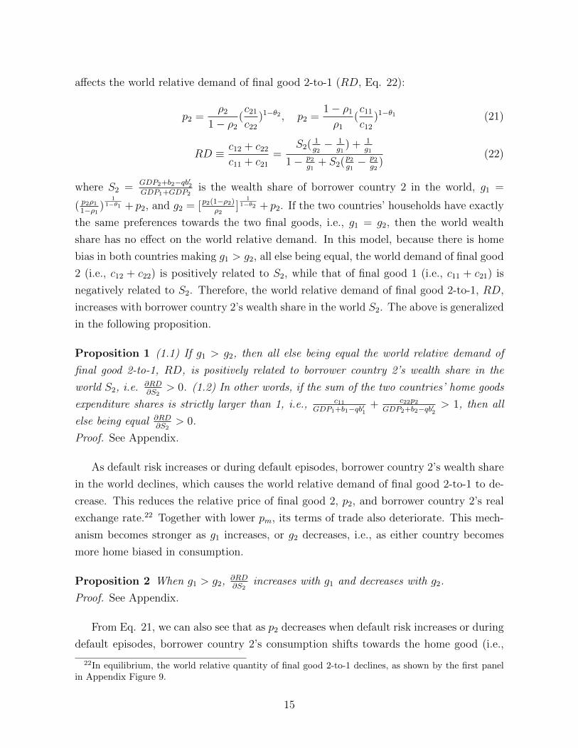
affects the world relative demand of final good 2-to-1 (RD, Eq. 22):
p2 =ρ2
1− ρ2
(c21
c22
)1−θ2 , p2 =1− ρ1
ρ1
(c11
c12
)1−θ1 (21)
RD ≡ c12 + c22
c11 + c21
=S2( 1
g2− 1
g1) + 1
g1
1− p2g1
+ S2(p2g1− p2
g2)
(22)
where S2 =GDP2+b2−qb′2GDP1+GDP2
is the wealth share of borrower country 2 in the world, g1 =
( p2ρ11−ρ1 )
11−θ1 + p2, and g2 = [p2(1−ρ2)
ρ2]
11−θ2 + p2. If the two countries’ households have exactly
the same preferences towards the two final goods, i.e., g1 = g2, then the world wealth
share has no effect on the world relative demand. In this model, because there is home
bias in both countries making g1 > g2, all else being equal, the world demand of final good
2 (i.e., c12 + c22) is positively related to S2, while that of final good 1 (i.e., c11 + c21) is
negatively related to S2. Therefore, the world relative demand of final good 2-to-1, RD,
increases with borrower country 2’s wealth share in the world S2. The above is generalized
in the following proposition.
Proposition 1 (1.1) If g1 > g2, then all else being equal the world relative demand of
final good 2-to-1, RD, is positively related to borrower country 2’s wealth share in the
world S2, i.e. ∂RD∂S2
> 0. (1.2) In other words, if the sum of the two countries’ home goods
expenditure shares is strictly larger than 1, i.e., c11GDP1+b1−qb′1
+ c22p2GDP2+b2−qb′2
> 1, then all
else being equal ∂RD∂S2
> 0.
Proof. See Appendix.
As default risk increases or during default episodes, borrower country 2’s wealth share
in the world declines, which causes the world relative demand of final good 2-to-1 to de-
crease. This reduces the relative price of final good 2, p2, and borrower country 2’s real
exchange rate.22 Together with lower pm, its terms of trade also deteriorate. This mech-
anism becomes stronger as g1 increases, or g2 decreases, i.e., as either country becomes
more home biased in consumption.
Proposition 2 When g1 > g2, ∂RD∂S2
increases with g1 and decreases with g2.
Proof. See Appendix.
From Eq. 21, we can also see that as p2 decreases when default risk increases or during
default episodes, borrower country 2’s consumption shifts towards the home good (i.e.,
22In equilibrium, the world relative quantity of final good 2-to-1 declines, as shown by the first panelin Appendix Figure 9.
15

c21c22
declines), while creditor country 1’s shifts towards the foreign good (i.e., c11c12
declines).
Hence, trade flows change.
To summarize, the main costs to the creditor when the borrower defaults are the
missed debt repayment, and the production loss caused by an efficiency loss in using
imported intermediate inputs from the defaulting country. These constrain the creditor
country’s budget. However, the creditor gains from more favorable terms of trade and real
appreciation that allow it to import more of the borrower country’s final good. For the
borrower country, the main costs upon default are wage losses, lower purchasing power,
and no access to the international bond market for consumption smoothing. It gains by
forgoing the debt repayment.
2.4.2 Equilibrium Bond Price
This section illustrates how bond prices are determined in the model. Figure 1 plots
bond price q against creditor country 1’s asset level tomorrow b′1 (i.e., borrower country
2’s borrowing tomorrow) for a given productivity state s and current asset level of the
creditor country, b1 (i.e., the borrower country’s current borrowing). In a simpler case
without default risk, the bond price is determined by the following equation in equilibrium:
q∗(b, b′, s) = β1
E1∂U∂c′11
λ1
= β2
E2∂U∂c′21
λ2
(23)
where λ1 = ∂U∂c11
and λ2 = ∂U∂c21
. The first equation is creditor country 1’s bond demand
function, and the second equation is borrower country 2’s bond supply function. As shown
in the left panel of Figure 1, the bond demand curve and bond supply curve (dashed lines)
are close to linear and intersect at point E1.23 Point E1 pins down the market equilibrium
bond price and tomorrow’s bond quantity.
If the current bond holding b1 is at a higher level, as in the right panel of Figure 1, then
bond demand curve will shift up (to the thicker dashed line) because of a lower current
marginal utility of domestic consumption (i.e., λ1), according to Equation 23. Meanwhile,
bond supply curve will shift down because of a higher current marginal utility of imported
consumption (i.e., λ2). The resulting new intersect point E1′ provides a larger equilibrium
bond quantity and a slightly lower price, depending on the two countries’ risk aversion.
Now let’s consider default risk. In equilibrium, bond demand and supply curves take
into account the borrower’s and the creditor’s perspectives on default probability, respec-
23Even in this risk-free bond case, the bond supply and demand curves are not exactly linear, becauseof the agents’ risk aversion.
16

Figure 1: Bond Price (given aggregate productivity state s)
Note: Dashed lines indicate that neither country considers default risk; solid lines indicate that bothcountries consider default risk but borrower country 2 is more optimistic about its repayment probability.The x-axis in the above plots is b′1. As b′1 is positive (right hand side) and becomes larger, borrowercountry 2 accumulates more and more debt.
tively, as in the following equations:
q∗(b, b′, s) = β1
∫s′ /∈D1(b′2)
∂U∂c′11∂U∂c11
dF1(s′|s) = β2
∫s′ /∈D2(b′2)
∂U∂c′21∂U∂c21
dF2(s′|s) (24)
When the two countries believe that default probability increases significantly, both
the demand and supply curves imply lower bond prices. It is reflected by the solid lines in
the left panel of Figure 1, given current b1, both curves bend downward as tomorrow’s b′1
(i.e., country 2 tomorrow’s borrowing) becomes larger. In particular, for borrower country
2, the intuition is that, taking default probability into account, the government knows it
has to lower the bond price in order to issue more bonds. But, as proven by Arellano
(2008), there is a lower bound for bond price q, up to which a borrower country is willing
to take on debt. That is, for any bond price q below a certain threshold, a borrower
country is able to issue less bond with a higher price q to finance the same amount of
consumption (of final good 1). Hence, the bond supply curve terminates at the lower
bound for q. The result is a different equilibrium point from the no-default-risk case, at
E2: both the equilibrium bond quantity and price are lower than those at E1.
Again, if the current bond holding is at a higher level, as indicated by the solid lines in
the right panel of Figure 1, then creditor country 1’s bond demand curve will shift upward
and borrower country 2’s bond supply curve will shift downward. The new intersect point
E2′, again, provides a larger equilibrium bond quantity and a lower price. However, owing
to the default risk, the increase in the bond quantity is much smaller and the decrease in
17

Figure 2: Default Probability Beliefs and Bond Price
Note: Here I assume that the creditor country always has the correct belief/concern about the defaultset and probability, i.e., D1 = D and π1 = π. Case (1) depicts the bond supply curve if borrowercountry 2 does not consider default probability when issuing bonds, used as baseline. Case (2)depicts the bond supply curve if the borrower country does consider default probability and is moreoptimistic about its repayment probability, or less concerned about default risk, than the creditorcountry is. Case (3) depicts the bond supply curve if the borrower country considers default probabilityand has the same belief or is more pessimistic about its repayment probability than the creditor country is.
the bond price is much larger than in the no-default-risk case.
However, Figure 1 only shows one special case of the two countries’ beliefs/concerns
about default probabilities, i.e., the bond supply curve starts to bend downward at a higher
bond quantity (b′1) than the bond demand curve does. It implies that when the bond is
initially issued, the borrowing government is more optimistic about making repayments,
or less concerned about default risk, than the creditor country is. The level of b′1 at
which the supply and demand curves start to bend down may differ depending on the
countries’ beliefs or concerns about the default probability. This issue does not arise in
small open economy sovereign default models because the borrowing government chooses
bond according to a price schedule following the creditor country’s bond demand curve.
Figure 2 shows three possible relations between the bond supply and demand curves,
assuming that the creditor country always has the correct belief about default risk and
default probability, i.e., D1 = D and π1 = π. The thick solid line (1) depicts the bond
supply curve when borrower country 2’s government does not consider default probability
when issuing bonds, i.e., D2 = ∅ or π2 = 0. It can be interpreted as follows: even though
the government aims to maximize the households utility in the long run, it is myopic on
debt repayments. Here I emphasize the timing of “when issuing bonds”, not after the
issuance. In reality, whether and when a borrower country’s government is not concerned
about sovereign default risk is difficult to verify. But given many countries’ serial default
events, it is possible that their governments learned little about their own default risk
18

from the past or were not concerned about the risk when issuing new bonds. A unique
equilibrium is guaranteed in case (1).
The thin solid line (2) depicts the bond supply curve when the borrower country does
consider default probability but is more optimistic about its repayment probability, or less
concerned about the default risk, than the creditor country is. This case also yields at least
one equilibrium.24 The dashed line (3) depicts the bond supply curve when the borrower
country considers default probability and has the same belief or is more pessimistic about
its repayment probability than the creditor country is, i.e., π = π1 ≤ π2 for each (s, b′2).
That is, the bond supply curve starts to bend down at the same time or earlier than the
bond demand curve does. This case, however, does not guarantee an equilibrium as in the
graph; the borrowing government may ration the supply of bonds. It is of future research
interest to investigate this case and look for the zone of such bond rationing.
This paper focuses on case (1) and (2), since they provide at least one equilibrium in
the bond market. I first solve case (1) as the baseline, then the optimistic borrower model
in case (2). In particular, for case (2) I specify that the borrowing government believes
its country has a higher steady-state productivity than the actual level that the firms and
the creditor country know. That is, all the agents in the model share the same default sets
D1 = D2 = D, but have different beliefs about default probabilities π = π1 > π2, since the
borrowing government is more optimistic about productivity on average. In reality, this
situation may stem from a developing country government’s overly optimistic perspective
on the country’s growth. Other scenarios can generate case (2) as well; I use the above
specification for its simplicity.25 I expect case (1) and case (2) to generate similar results.
3 Quantitative Results
3.1 Baseline Calibration
In this section, I study the quantitative implications of the model by conducting numerical
simulations at the quarterly frequency and using a baseline calibration based on the data,
largely from Mexico and Canada. Table 1 shows the calibrated parameter values.26
24The equilibrium is unique as long as line (2) does not bend down to cross the bond demand curveagain. It depends on the slope of both curves. When both countries hold the same beliefs about thestandard deviation and the transition probabilities of the borrower’s productivity shocks, the equilibriumis unique.
25For example, the borrowing government may not be concerned about default risk until its debt levelreaches a certain level.
26U.S. is Mexico’s number 1 trade partner and creditor, while Canada is also among the top 6 since1980s.
19
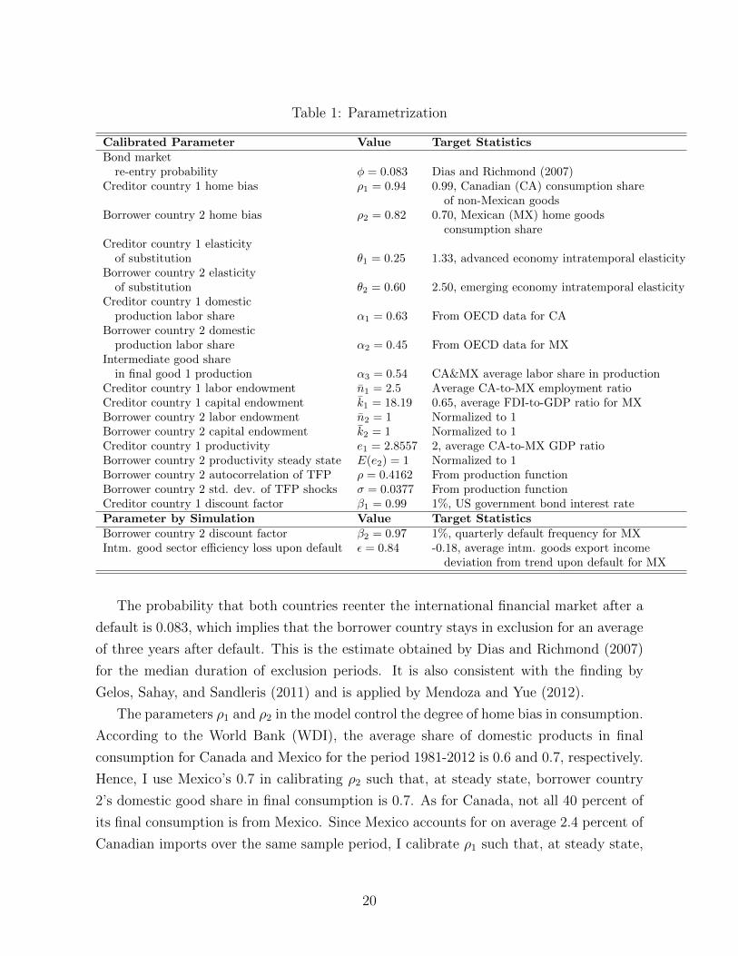
Table 1: Parametrization
Calibrated Parameter Value Target StatisticsBond market
re-entry probability φ = 0.083 Dias and Richmond (2007)Creditor country 1 home bias ρ1 = 0.94 0.99, Canadian (CA) consumption share
of non-Mexican goodsBorrower country 2 home bias ρ2 = 0.82 0.70, Mexican (MX) home goods
consumption shareCreditor country 1 elasticity
of substitution θ1 = 0.25 1.33, advanced economy intratemporal elasticityBorrower country 2 elasticity
of substitution θ2 = 0.60 2.50, emerging economy intratemporal elasticityCreditor country 1 domestic
production labor share α1 = 0.63 From OECD data for CABorrower country 2 domestic
production labor share α2 = 0.45 From OECD data for MXIntermediate good share
in final good 1 production α3 = 0.54 CA&MX average labor share in productionCreditor country 1 labor endowment n1 = 2.5 Average CA-to-MX employment ratioCreditor country 1 capital endowment k1 = 18.19 0.65, average FDI-to-GDP ratio for MXBorrower country 2 labor endowment n2 = 1 Normalized to 1Borrower country 2 capital endowment k2 = 1 Normalized to 1Creditor country 1 productivity e1 = 2.8557 2, average CA-to-MX GDP ratioBorrower country 2 productivity steady state E(e2) = 1 Normalized to 1Borrower country 2 autocorrelation of TFP ρ = 0.4162 From production functionBorrower country 2 std. dev. of TFP shocks σ = 0.0377 From production functionCreditor country 1 discount factor β1 = 0.99 1%, US government bond interest rateParameter by Simulation Value Target StatisticsBorrower country 2 discount factor β2 = 0.97 1%, quarterly default frequency for MXIntm. good sector efficiency loss upon default ε = 0.84 -0.18, average intm. goods export income
deviation from trend upon default for MX
The probability that both countries reenter the international financial market after a
default is 0.083, which implies that the borrower country stays in exclusion for an average
of three years after default. This is the estimate obtained by Dias and Richmond (2007)
for the median duration of exclusion periods. It is also consistent with the finding by
Gelos, Sahay, and Sandleris (2011) and is applied by Mendoza and Yue (2012).
The parameters ρ1 and ρ2 in the model control the degree of home bias in consumption.
According to the World Bank (WDI), the average share of domestic products in final
consumption for Canada and Mexico for the period 1981-2012 is 0.6 and 0.7, respectively.
Hence, I use Mexico’s 0.7 in calibrating ρ2 such that, at steady state, borrower country
2’s domestic good share in final consumption is 0.7. As for Canada, not all 40 percent of
its final consumption is from Mexico. Since Mexico accounts for on average 2.4 percent of
Canadian imports over the same sample period, I calibrate ρ1 such that, at steady state,
20

creditor country 1’s domestic good share in final consumption is 0.99.
The next two parameters θ1 and θ2 have to do with the elasticity of substitution
between domestic good consumption and imported good consumption for developed and
developing countries.27 The literature provides a large range of estimates for the elasticity
of substitution. Backus, Kehoe, and Kydland (1994) document that U.S. elasticity is
between 1 and 2; values in this range are commonly used in empirical trade models.
Their benchmark model adopts a value of 1.5. Later authors have used similar values,
e.g., Chari, Kehoe, and McGrattan (2002), Bergin (2006), and Ruhl (2008). A recent
paper by Feenstra, Luck, Obstfeld, and Russ (2014) also find point estimates for the
macro elasticity exceeding unity in almost all industries.
However, few papers have studied the Armington elasticity for developing countries.
Ostry and Reinhart (1992) find the elasticity of substitution between traded and nontraded
goods in the range of 1.22 to 1.27, and significant regional differences, with less-developed
countries displaying higher values. Yet, the cross-country comparison of Armington elas-
ticities remains unclear. This paper does not take a stand on the value of the elasticity.
As a starting point, I adopt 1.33 as the elasticity of substitution for the creditor coun-
try to match that for developed countries on average, and a higher value of 2.5 for the
borrower country to indicate that less-developed countries may have a higher elasticity of
substitution between home and foreign goods as they do for traded and nontraded goods.
In sensitivity analyses, I explore other values for the elasticities.
The labor share in the final good production is set at 0.63 for Canada and 0.45 for Mex-
ico, which are the average labor income shares using annual data for the period 1981-2009
(1981-2008 for Canada) from OECD Statistics. The input share of imported intermediate
good to produce final good 1 is the average labor share in final good production of Canada
and Mexico. I vary this parameter value in sensitivity analysis as well.
The capital and labor endowments of borrower country 2 are normalized to 1. Hence,
creditor country 1’s labor size is n1 = 2.5 to match the average CA-to-Mexico employment
ratio for 1981Q1-2012Q4. Creditor country 1’s capital endowment k1 is chosen such that,
at steady state, its capital used with the intermediate good, km, is 65 percent of borrower
country 2’s GDP. This is approximated by the average of FDI-to-GDP ratio for Mexico
during 1981Q1-2012Q4, assuming the majority of the FDI to Mexico is vertical. However,
it is important to note that this approximated target is by no means a complete calibration
for the actual amount of foreign capital used with Mexican intermediate goods to produce
foreign final goods.
27Without default risk, θ1 and θ2 also determine the values for the elasticity of intertemporal substi-tution for both countries. But with default risk, the intertemporal elasticity decreases with the risk.
21

The only productivity shock in the model is to borrower country 2’s productivity e2,
whose steady state is normalized to 1. It follows an AR(1) process:
log e2,t = ρ log e2,t−1 + ηt
with η being iid and following N(0, σ2). I estimate the process using the model’s pro-
duction functions, and HP-filtered Mexican data for GDP, (average) capital stock, and
employment in both the domestic sector and the FDI sector for 1981Q1-2012Q4. Using
the method proposed by Tauchen and Hussey (1991), I construct a Markov approximation
to this process with 5 states of productivity realization for e2. For creditor country 1,
its constant productivity e1 is calibrated to be 2.8557, so that at steady state the CA-
to-Mexico GDP ratio is 2, equal to the average CA-to-Mexico GDP ratio for 1981-2011,
according to IMF annual data.
Both U.S. and Canadian treasury bills bear real interest rates that are below 1 percent
on average; hence we have β1 = 0.99. Last, the targets for setting β2 and ε are quarterly
frequency of Mexican defaults and the loss in Mexican intermediate goods exports upon
default. Mexico’s quarterly default frequency is 1%, since it had eight default episodes
between 1828 and 2012 according to Reinhart (2010). In the later sections, to study
the dynamics around Mexican sovereign defaults during the 1980s, I include more such
episodes from Paris Club data for the sample period 1981Q1-2012Q4. They are 1982Q3,
1986Q1, and 1989Q1. At the onset of these most recent sovereign default episodes, Mex-
ico’s intermediate goods export value, on average, was about 18 percent below trend.
Given these two targets, the simulated procedure yields β2 = 0.97 and ε = 0.84.
I solve the model with a discretized state space of 5 realizations for borrower country
2’s productivity and 107 points for asset holdings. The model is considered to be solved
when the convergence distance diminishes to 1.0000e − 06. In the following sections, I
first examine the properties of the calibrated model and then study the simulated results,
both over business cycles and around default events.
3.2 Policy Functions
The properties of bond quantity and its price in the baseline model are in line with other
sovereign default papers. The left plot in Figure 3 graphs the next-period assets for
the borrower country against its current assets, in a high-productivity state and a low
productivity state in the current period. As the borrower country accumulates debt (to
the left of the bottom axis), its marginal borrowing capacity diminishes. Moreover, when
22

the country is in a low-productivity state, its bond function starts to flatten out at a lower
current debt amount than it would in a high-productivity state. That is to say, all else
being equal, a higher productivity state supports a higher debt level.
Figure 3: Policy Functions
The right plot in Figure 3 graphs the bond price functions. It shows that the bond
price decreases with the debt level (i.e., interest rate rises). Across productivity states,
the bond price is significantly higher for a high-productivity state, which implies that
interest rates are countercyclical.
3.3 Cyclical Movements
This section starts the assessment of the quantitative performance of the model by com-
paring moments from the data with moments from the model’s dynamics. To compute
the latter, I feed borrower country 2’s productivity process into the model and conduct
1,000 simulations, each with 600 periods. Then I truncate the first 100 observations and
use the rest to compute the statistics of the model results.
Table 2 compares the moments produced by the baseline model and optimistic bor-
rower model with those from Mexican data and from Mendoza and Yue (MY, 2012). All
the data used in this model are quarterly from 1981Q1 to 2012Q4. The data sources
are provided in the Appendix. Note that Mendoza and Yue (2012) calibrate their model
partially to Argentine data and partially to Mexican data.
As explained earlier, to guarantee the existence of bond market equilibrium, on one
hand, the baseline model assumes that the borrowing government is unconcerned about
default probability (i.e., D1 = D, π1 = π, and D2 = ∅ or π2 = 0, as case (1) in Figure
3). On the other hand, the optimistic borrower model assumes that the government does
23

Table 2: Statistical Moments of Borrower Country 2’s Business Cycles
Statistics Data Baseline M&Y Optimistic(2012) Borrower∗
Average debt/GDP ratio (in percent) 74.94 27.44 22.88 27.43Average bond spreads (in percent) 4.35 4.59 0.74 4.59Bond spreads std. dev. (in percent) 4.71 2.44 1.23 2.48Real exchange rate std. dev. (in percent) 17.30 ∗∗∗1.99 n.a. 2.03Terms of trade std. dev. (in percent) 6.21 ∗∗∗3.87 n.a. 3.95Dom. product con. std. dev./GDP std. dev. 1.23 0.96 n.a. 0.96Total consumption std. dev./GDP std. dev. 1.12 1.09 1.05 1.09Trade balance/GDP std. dev. (in percent) ∗∗2.08 1.40 n.a. 1.41Correlation with GDP
Bond spreads −0.39 −0.92 −0.17 −0.92Real exchange rate 0.53 ∗∗∗0.54 n.a. 0.55Terms of trade 0.25 ∗∗∗0.49 n.a. 0.50Trade balance/GDP ∗∗ − 0.65 −0.20 −0.54 −0.19Total exports 0.21 0.85 n.a. 0.85Intermediate good exports 0.18 0.85 n.a. 0.85Total import 0.75 0.92 n.a. 0.92Wage 0.65 0.88 n.a. 0.87GDP volume 0.65 0.79 n.a. 0.79Default occurrence −0.14 −0.24 −0.09 −0.24Default duration −0.39 −0.64 n.a. −0.64
Correlation with bond spreadsReal exchange rate −0.76 ∗∗∗ − 0.78 n.a. −0.79Terms of trade −0.13 ∗∗∗ − 0.77 n.a. −0.77Trade balance/GDP ∗∗0.30 0.50 0.15 0.50Total exports −0.02 −0.63 n.a. −0.63Intermediate good exports −0.08 −0.65 n.a. −0.64Total import −0.28 −0.91 n.a. −0.91Wage −0.35 −0.68 n.a. −0.68GDP volume −0.19 −0.52 n.a. −0.51Default occurrence 0.18 0.26 n.a. 0.26Default duration 0.56 0.86 n.a. 0.86
Note: All data in the table are HP-filtered, except bond spreads and default occurrence and duration.
All data are in real terms and at quarterly frequency. Bond spreads are calculated over U.S. government
bond real interest rates that are sometimes negative. ∗Under optimistic borrower case, the government
believes E(e2) = 1.04 with all else being the same as the baseline calibration. That is, the government-
perceived average productivity is about one standard deviation higher than the actual level. ∗∗Mexican
bilateral trade balances with Canada exhibit similar statistics as Mexican total trade balances’ statistics,
except with smaller magnitudes. ∗∗∗I use Laspeyres price index for CPI and real exchange rates, and unit
value index for terms of trade. Under Paasche price index, the correlations and standard deviations of
real exchange rates remain the same or increase slightly without switching signs.
24

consider default probability but believes its country has a higher steady-state productivity
than the actual level that the firms and the creditor country know (i.e., D1 = D2 = Dbut π = π1 > π2, as case (2) in Figure 3). More specifically, The borrowing govern-
ment believes E(e2) = 1.04 with all else being the same as the baseline calibration; that
is, the borrowing government perceived average productivity is about one standard de-
viation higher than the actual level. Although these two cases differ in the borrower’s
belief/concerns regarding default risk, they have similar results, as expected and illus-
trated in Figure 3. Unless otherwise stated, the analysis for the rest of this paper is based
on the baseline model results.
Table 2 shows that this model produces a debt-to-GDP ratio of about 27 percent
on average, while matching the 1 percent default frequency observed in the data. The
result that the debt-to-GDP ratio is lower than the data is common in the literature of
strategic sovereign default models. There are several main factors impacting this ratio
in the model, including the two countries’ discount factors, beliefs on default probability,
sovereign default costs, and risk aversion. In particular, risk aversion limits this model’s
ability to generate data-matching debt-to-GDP ratios (Lizarazo, 2013). However, it does
help my model support a data-consistent average bond spread, on which I elaborate below.
Model statistics for bond spreads are tricky in that during default periods the model
has no finite interest rate. I report in Table 2 the modeled bond spread statistics for
business cycles, with the infinite interest rates during default episodes being replaced by
the average Mexican counterpart from the data (10 percent). The mean of bond spreads
is close to the data. Here, the bond price reflects not only the expected return due
to the probability of default, but also compensation to risk-averse creditors for bearing
sizable consumption risk.28 On average about a third of the interest rate is attributed
to the risk premium from creditor’s risk aversion. 29 The impact of risk aversion on
the risk premium decreases relative to the impact of default risk as the borrower country
approaches a default. Therefore, unlike many previous studies using small open economies
with risk-neutral investors, this model breaks the close link between the probability of
default and bond pricing by including the creditor country’s welfare loss and risk aversion.
Meanwhile, the modeled volatility of bond spreads is smaller than the data.
In the model, the volatility of terms of trade is closer to the data than the volatility
28As explained in the next section, the creditor country suffers a long-lasting welfare decline once theborrower country defaults. The impact of the creditor country’s welfare loss on bond spreads followsa similar rationale of “rare disaster” as in Barro (2006) and Gabaix (2008), and is consistent with thefindings of Lizarazo (2013).
29To estimate that, I calculate the bond price without default risk as q(b, b′, s) = β1E1
∂U∂c′11λ1
, given thecurrent model result b′.
25

of real exchange rates is. When default risk increases or during default episodes, even
though the borrower country’s terms of trade deteriorate and its CPI declines, the creditor
country also adjusts its consumption towards the cheaper imported final good. It results in
a lower CPI for the creditor country as well, causing the borrower country’s real exchange
rate does not decline as much as its terms of trade do. Meanwhile, in the data, both the
terms of trade and the real exchange rate are influenced by many other factors during
business cycles, such as policies in trade, money supply, and nominal exchange rate, which
this model does not take into account.
Domestic good consumption is smoother in the model than in the data because of
borrowing, home bias preference, and labor movement from the intermediate good sec-
tor to the domestic sector during default crises. These three factors support domestic
good production and their consumption in spite of adverse productivity shocks. Total
consumption is less smoothed than domestic good consumption in the model on account
of the variations in imports and terms of trade over business cycles. It is also slightly
more volatile than output, as in the data. The volatility of trade balances is lower in the
model than in the data. Other sovereign default models have generated similar results.
For example, Aguiar and Gopinath (2007) produce a trade balance standard deviation of
0.95, Arellano (2008) 1.5, and Yue (2010) 2.81.
Next, Table 2 shows that this model does a good job of delivering the correlation
between GDP value and bond spreads, as well as their correlations with other variables.
It yields a negative correlation between bond spreads and GDP, consistent with the data,
because bonds have a higher default risk in bad states. As in Mendoza and Yue (2012), this
model produces countercyclical default risk in a setting where both income and default
risk are endogenous and affect each other, unlike in the models of sovereign default alone
or of business cycles alone.
However, this model distinguishes itself from Mendoza and Yue (2012) in that the
endogenous income and default risk interact through the movement of terms of trade. In
my model, both the terms of trade and the real exchange rate have a positive relation to
GDP and a strong negative relation to bond spreads, which is also consistent with the data.
As explained in the model mechanism section, when the borrower country accumulates
debt, the default risk and the interest rate rise, resulting in the country’s terms-of-trade
deterioration. This prevents real appreciation from easing its budget constraint and from
helping it to pay back debt that is denominated in the creditor country’s final good.
Therefore, default risk is further elevated to raise the bond interest rate. Once an adverse
productivity shock causes the borrower country to default, the country is penalized by an
additional income loss from a wage decline, causing its terms of trade and real exchange
26

rate to deteriorate sharply. This takes a third toll on the defaulting country’s income.
This mechanism, in which increased debt and default risk raise the real interest rate,
deteriorate terms of trade, real exchange rate, and income, explains the modeled relations
between GDP value, bond spreads, terms of trade, and real exchange rates. It also explains
the model-generated negative relation between trade balances and GDP, while producing
a positive relation between trade balances and bond spreads. These are consistent with
the stylized business cycle features in Mexico and other developing countries.
More important, the model also delivers procyclical trade flows and a negative relation
between trade flows and bond spreads consistently with the data, which have not been
captured by previous sovereign default models. During downturns, the value of both
imports and exports declines, partly because of the deterioration in the terms of trade.
Furthermore, the model predicts a correlation between the borrower country’s exported
intermediate good and its GDP or bond spreads, qualitatively in line with the correlations
observed in the Mexican data. More broadly, the business cycle correlations between
output and intermediate goods export value differ across countries but are usually positive.
For instance, using annual growth data (1988-2013), I compute the correlation for 16
countries for which I have intermediate goods export data. On average, the correlation
between output growth and intermediate goods export growth is 41 percent.30
As discussed earlier, the wage in borrower country 2 declines with productivity and
even more so during sovereign default episodes. It is confirmed by the model results, where
the wage strongly positively correlates with GDP and negatively with bond spreads, as
in the data and the findings of Li (2011).
In addition, this model disentangles the default-related loss of GDP volume in GDP
value. As I show in the next section, during default periods, about two thirds of GDP
value loss in the model is due to lower GDP volume, while the other third is attributable
to real depreciation. In Table 2, even though GDP value is positively correlated with
GDP volume, it is not a perfect correlation–only 65 percent in the data and 79 percent in
the model. The real exchange rate and terms of trade do play a role in explaining GDP
value changes in both the model and the data. Also, consistent with the data, the model
generates declining GDP volume when bond spreads increase over business cycles.
Last, I report in Table 2 the correlations between default and output, and between
default and bond spreads. In particular, the onset of a default event is positively correlated
30The correlation for Argentina is 34.8%, Brazil 66.4%, Croatia 13.1%, Ecuador 5.2%, Greece 17.1%,Iceland 41.8%, Indonesia 24.4%, Moldova 26.2%, Peru 52.6%, Russia 66.1%, South Africa 56.4%, Thailand55.5%, Turkey 7.2%, Ukraine 81.8%, Uruguay 58.5%, and Venezuela 43.3%. Using HP-filter, the averagecorrelation is 33%.
27
with output and negatively correlated with bond spreads in both the data and the model.
As for the duration of a default episode, it is more closely related to bond spreads than
to output in the model, which is also the case in the data.
3.4 Dynamics around Default Events
Next I study the baseline model’s macroeconomic, trade, and welfare dynamics of borrower
country 2 around default events by comparing the simulated results with the time series
data for Mexico. In this paper I identify three sovereign defaults by Mexico since 1981,
in 1982Q3, 1986Q1, and 1989Q1. Those dates are inferred from Paris Club data, which
shows that Mexico was treated on 22 June 1983, 17 September 1986, and 30 May 1989 by
foreign creditors for its sovereign debts.31 Each episode window covers 6 quarters before
and after the onset of a default.32 Date 0 is the quarter in which the default occurs. I
plot the mean of these three default episodes for each variable from the data, as well as
the mean from the model simulation surrounded by a one-standard-deviation band.33
3.4.1 Macroeconomic Dynamics
Figure 4 shows the model’s macroeconomic dynamic results, i.e., deviations from the
steady state of borrower country 2, compared with Mexican data and the mean of all
sample countries (see the Appendix for the list of countries). In the model, the sharp
decline (13 percent below trend) and the slow recovery of GDP value (in creditor country
1’s final good 1) match well with those of the real GDP value data (in USD) for Mexico.
In the model, the decline of income upon default comes from two sources: GDP volume
decrease and real depreciation. First, Mexico’s GDP volume (seasonally adjusted) does
not seem much affected by the default events, whereas in the model GDP volume decreases
by about 10 percent on average.34
Second, on average, the terms of trade deterioration after a default in the model is
consistent with the data. But the data also show a faster recovery of terms of trade
than the model results. The model’s real exchange rate declines slightly less than the
31Slight sovereign default date adjustments according to GDP fluctuations have been made with regardto the Paris Club dates to reflect delayed treatments after defaults. The results are not sensitive to thedefault date specifications.
32The length of 6 quarters is chosen because the three Mexican sovereign default are separated byabout three years; and 6 quarters is the middle point.
33This section uses the same simulation results as the previous section.34Small reductions in GDP volume around the default episodes for Mexico are not uncommon in other
countries. The changes in GDP volume growth upon default differ across countries. For instance, GDPvolume in Paraguay grew by 4.32 percent during its 2003 default, while Indonesia’s GDP volume declinedby 13.13 percent during its 1998 default.
28

Figure 4: Macroeconomic Dynamics of Borrower Country 2 around Default Events
Note: Default events are identified as occurring in 1982Q3, 1986Q1, and 1989Q1. Except for the interest rate and debt-to-GDP ratio, all other data are HP-filtered. GDP value (in USD), GDP volume, terms of trade, domestic sector labor, hoursworked, and intermediate goods export sector (FDI) labor are logged before being detrended. All data are real. For thesubplots with a different scale on the right axis, the scale is for the data of the variable. The model results for GDP valueare measured in creditor country 1’s final good 1. The dotted line in the Domestic Sector Labor plot is Mexico’s data ontotal hours worked.
29
terms of trade and the data do. As explained in the section of business cycle results, the
creditor country’s consumption adjustment moderates the decline in the real exchange
rate. In addition, in this model the nominal exchange rate is fixed at one, whereas in
reality it usually changes with each sovereign default episode. Therefore, the decline of
real exchange rate is limited in this model. Overall, the real GDP loss upon default is
driven by the deterioration of the terms of trade and the real exchange rate as well as the
decline in production activity in the model, and even more so by the real depreciation in
the Mexican data.
In the sovereign debt market, the model matches well the increase in the real interest
rate around default events. I do not show the model interest rate at the default quarter
because it does not exist due to the country’s exclusion from the bond market.35 On
average, the model is able to support high real interest rates and bond spreads that not
only incorporate the default risk, but also compensate the creditor country for its welfare
loss and risk aversion.
Moreover, this model predicts that the debt-to-GDP ratio is relatively stable over
the four quarters prior to a default, then surges as it approaches and reaches default,
and drops afterwards. To make the model’s debt ratio comparable to the data, I follow
Mendoza and Yue (2012) and adjust the mean of the post-default debt ratios from the
model to be the average of the pre-default debt ratio and the debt ratio chosen once the
countries re-enter the bond market. However, the adjusted post-default debt ratio in the
model still declines faster than in the data. Also, the model’s debt ratio is lower than the
data’s, which is an issue common to the previous strategic sovereign default models.
In addition, the model produces the qualitative feature of the employment decline in
the intermediate good exports sector. The pattern is consistent with the finding of Bergin,
Feenstra, and Hanson (2009, 2011).36 But the model does not match the domestic final
good sector employment, for two reasons. One reason is that the model does not in-
clude unemployment. More specifically, the borrower country’s domestic final good sector
employs whoever are not hired by intermediate good sector. If this limitation were elimi-
nated, the model could potentially have another labor market channel affecting the costs
of default for the borrower country, as in Mendoza and Yue (2012). However, the exclu-
35Not all of the periods immediately after the sovereign default quarter have interest rates because thecountries can only re-enter the bond market with a certain probability. I therefore show the statistics forcases in which the countries re-enter shortly, and for those have not re-entered yet, I cap the interest rateat Mexican average interest rate during default episodes (10 percent).
36Bergin, Feenstra, and Hanson (2009, 2011), using Mexico’s maquiladora sectors, find that the coun-try’s offshoring industries experience employment fluctuations that are much more volatile than those inthe U.S.
30
sion of unemployment may not be a significant factor, since the Mexican unemployment
rate is relatively low at 3.8 percent on average (1980-2012).
The second reason is that the employment data here poorly captures informal sector
employment in Mexico in the early 1980s. Fernandez and Meza (2014), using data since
1987, document that informal sector employment accounts for about half of Latin Amer-
ican employment and is strongly countercyclical and negatively correlated with formal
employment in Mexico. If informal sector employment were included in the data in Fig-
ure 4, the decline in employment during Mexico’s defaults would be milder. Furthermore,
if we look at total hours worked (the dotted line), it did not decline as much as employ-
ment upon default.37 Overall, I simplify the labor market in this paper to highlight the
terms-of-trade channel and international trade results.
3.4.2 Trade Dynamics
I analyze the model’s performance for variables related to international trade in Figure
5. In the model, borrower country 2’s total export value (measured in creditor country
1’s final good) declines, but more than data do. For intermediate good exports, their
value declines initially upon default in the model, as in the data. It is worth noting that
intermediate good exports performing below trend is not uncommon in other developing
countries’ default episodes, as shown in Figure 5’s all country mean data line.
Figure 5 also plots the dynamics for imports and total trade. The model does well in
matching the import data upon default, given that most of the data path is within the
error bands of the model result. Adding import value and export value together, total
trade value declines, which is consistent with the finding of Rose (2005).
More trade volume dynamics are reported in Figure 8 in the Appendix. There it shows
that this model also generates data-consistent declining intermediate good export volume
and import volume upon default. However, the modeled total export volume declines
much more than in the data. This implies that the majority of the modeled changes of
total export value come from the volume changes, while a small portion comes from the
terms-of-trade deterioration, which need improving in future studies.
3.4.3 Creditor Country and Welfare Dynamics
Since this paper uses a two-country model, I can study the welfare of both the creditor and
the borrower (Figure 6). For the creditor country, the model predicts a persistent decline
37Note that, owing to data limitations, data for total hours worked are for the manufacturing sector,not necessarily for domestic final goods production only.
31

Figure 5: Trade Dynamics of Borrower Country 2 around Default Events
Note: Default events are identified as occurring in 1982Q3, 1986Q1, and 1989Q1. All data are real, logged, and HP-filtered.The model results for export values are measured in creditor country 1’s final good 1.
of output about 0.4 percent below trend upon the borrower country’s default, due to
inefficiency in production operations with the imported intermediate good. The result is
close to that in Canadian output data during the Mexican post-default sample episodes.38
Moreover, this model generates a default-triggered welfare decline of 0.04 percent for the
creditor country; this loss remains negative and slowly declines to zero during the next 6
quarters and beyond. The magnitude of the damage to the creditor country, however, is
much smaller than that to the borrower country (a 0.34 percent decline in welfare), but
the effect on the creditor is longer lasting than that on the borrower.
The welfare decline is mainly because the creditor country’s budget is tightened when
the borrower country defaults in its debt repayment, and it suffers income losses from
reduced production. However, favorable terms of trade reduce the pain to creditor country.
Yet by no means should we take the welfare numbers reported here literally. In practice,
the impact of a sovereign default on a creditor country’s welfare depends on many other
38In the data, shocks originated from Canada potentially can affect Mexico during the latter country’sdefault episodes as well. Since this model does not contain the cross-country spillover effect, it cannotaddress the endogenous issue.
32

Figure 6: Creditor Country and Welfare around Default Events
Note: Default events are identified as occurring in 1982Q3, 1986Q1, and 1989Q1. All data are real,logged, and HP-filtered.
factors. For instance, it hinges on the substitutability between imports from the defaulting
country and other goods for consumption and production in the creditor country.
For the borrower country, a default triggers, on average, a 0.34 percent drop in welfare.
It comes primarily from the endogenous income reduction. But this welfare loss can be
recovered in fewer than 6 quarters, as the borrower country shifts labor to domestic sector
that supports post-default domestic final good consumption and exports. In the model, a
default also causes the world welfare to decline. In the Appendix, I also show the baseline
model result can replicate the time series of Mexico’s output and bond spreads for the
sample period 1981Q1-2012Q4.
3.5 Sensitivity Analysis
In this section I conduct a sensitivity analysis to evaluate the robustness of the baseline
model’s quantitative results regarding the terms of trade, the real exchange rate, bond
spreads, and trade flows. The model results are robust to changes in the data filter (BP-
filter), the borrower country’s shock persistence (ρ), patience (β2), post-default efficiency
loss in the intermediate good exports (ε), elasticities of substitution ( 11−θ1 ,
11−θ2 ), and the
creditor country’s imported intermediate good input share (α3). The first three robustness
reports are detailed in the Appendix, while the rest are in this section. This section also
empirically checks the model results with assumptions violating Proposition 1 to show
the importance of home bias in consumption. All the sensitivity analysis results are
summarized in Table 4 and Table 5 in the Appendix.39 Those tables report the main
39I also generated around-default dynamics plots comparable to Figure 4–6. The quantitative differ-ences are small and the qualitative patterns are the same, so I do not include them in the paper due tospace limitation. But several around-default values for variables of interest are reported in Table 4 andTable 5.
33
business cycle statistical moments as in Table 2 for each scenario, plus default frequency
and several around-default statistics for variables of interest.
3.5.1 Post-default Efficiency Loss in Intermediate Good Export Sector
First, I report results with a lower value of ε = 0.81 (i.e., a greater efficiency loss in
production operations with the imported intermediate good upon default) and a higher
ε = 0.87 than that in the baseline ε = 0.84 in Table 4 in the Appendix. It is important
to experiment with different values of ε because it governs the magnitude of post-default
losses in the demand of the defaulting country’s intermediate good, and thus also losses in
its income, terms of trade, real exchange rates, and trade flows. Even though the results
change slightly under different values of ε, the signs of all the statistics remain consistent
with the data.
A lower value of ε = 0.81, i.e., a larger efficiency loss, induces two main effects.
First, it helps the borrower to maintain a higher average debt-to-GDP ratio. Second,
together with the home bias preference, a larger decline in intermediate good demand
and a tighter budget make the borrower’s trade flows, terms of trade, and real exchange
rates more responsive to a default crisis. Thus, the volatility of the real exchange rates
and trade balances are higher, as are their correlations with GDP and bond spreads.
As for welfare, given a higher efficiency loss (i.e., ε = 0.81), one would expect to cost
the borrower more upon default. However, with a higher average debt-to-GDP ratio, the
borrower also benefits more from forgoing a larger debt repayment, so its welfare does not
lose as much than in the baseline. Meanwhile, the creditor loses more from a larger debt
default and a larger efficiency loss in operations. Hence, the world’s total welfare loss
is lower than that of the baseline. This result implies that policies to limit the default-
triggered damages in foreign business environment in the defaulting country can reduce
both countries’ welfare losses upon default.
3.5.2 Intermediate Input Share
Next, I vary the intermediate input share in final good 1’s production to examine the effect
of changes in α3 (baseline α3 = 0.54). With a larger intermediate input share (α3 = 0.56),
final good 1’s production becomes more affected by the efficiency loss in operations with
intermediate inputs from the borrower country. This amplifies the impact of a sovereign
default on terms of trade and real exchange rate. We can see that they become more
volatile and responsive to output and bond spreads, than in the baseline. However,
greater vertical integration also reduces the world welfare losses upon default.
34

3.5.3 Home Bias
The fifth column of Table 5 in the Appendix displays the model result if both countries’
households have exactly the same preference towards the two final goods, i.e. ρ1 = ρ2 =
0.5 and θ1 = θ2 = 0.5.40 In this case, g1 = g2, the world relative demand for final goods is
no longer subject to changes in the countries’ relative wealth share. Hence, I expect the
final good relative price p2 to increase upon default, so do terms of trade.
The results show that for the borrower country: (1) its terms of trade are negatively
associated with GDP value, and positively associated with bond spreads, (2) its terms
of trade slightly improve upon default, and (3) its real exchange rate is also negatively
associated with GDP value, but only weakly negatively associated with bond spreads.
The middle panel in Figure 9 in the Appendix also confirms these results by displaying a
rise in terms of trade around a default event. All these results contradict the data. This
is why the two countries’ home bias preferences in consumption play a crucial role in the
model to generate data-consistent results.41
3.5.4 Armington Elasticities of Substitution
Finally, I check the robustness of the elasticities of substitution between home and im-
ported final goods for both countries. When the substitutability in the borrower coun-
try decreases (θ2 = 0.56), imports are less replaceable by the domestic final good in a
downturn when the terms of trade deteriorate. Therefore, the borrower country defaults
slightly less frequently to avoid terms-of-trade deterioration, and it borrows more. It also
suffers a smaller welfare loss upon default. In the last column of Table 5, when I change
both countries’ elasticities of substitution to 2 (Backus, Kehoe, and Kydland, 1994) and
re-calibrate the entire model, the results are consistent with the baseline.
More sensitivity analysis results are detailed in the Appendix. Summing up, the
sensitivity analysis shows that although the model’s statistical moments vary somewhat
when I change key parameters, the main quantitative and qualitative findings are robust
to these changes. The model produces a decline in terms of trade upon default, a high
average bond spread, a negative correlation between trade balances and GDP, and other
data-consistent correlations between trade flows and GDP or bond spreads.
40In this case, borrower country 2 has no home bias in consumption, while creditor country 1 consumesmainly the home good.
41Alternatively, one could use international trade cost to generate the same impact as home bias.
35

4 Conclusion
This paper proposes a two-country model of sovereign default, including production ver-
tical integration and consumption home bias. It contributes to the literature by exploring
the role of vertical integration to affect sovereign debt contracts prior to default events
and income losses during debt crises for both creditor and borrower countries. The model
also contributes to sovereign default theory by generating endogenous trade flows, terms
of trade, and real exchange rate that interact with default risk, as well as generating their
deterioration upon default. Its quantitative results are consistent with observed empirical
regularities around Mexico’s sovereign default events and over its business cycles.
The model features a terms-of-trade amplification channel that links sovereign default
risk and events with trade and income. As a country borrows more and more, its default
risk and interest rate increase, its income declines, and its terms of trade deteriorates,
which in turn reduces the borrower country’s income and raises its default risk. Once the
borrower does default, its income declines further, its terms of trade and real exchange
rate deteriorate sharply. This real depreciation then takes another toll on the defaulter’s
income and trade values. This term-of-trade channel produces a novel feedback loop
among the borrower’s sovereign default risk and occurrences, income, and trade.
The model results are consistent with three important stylized facts of emerging mar-
kets’ business cycles and sovereign defaults. First, it delivers countercyclical trade bal-
ances and procyclical trade flows over business cycles. Second, it produces countercyclical
bond spreads with a data-consistent average. Third, this model accounts for sharp de-
terioration in the terms of trade and the real exchange rate, and reductions in trade
flows upon default. Moreover, the model does not need an exogenous endowment loss
following a sovereign default, but endogenously generates GDP losses, partially from real
depreciation, partially from production activity decrease, as in the data.
This model also predicts small but long-lasting welfare losses for the creditor country,
and relatively large but short-lived welfare losses for the borrower country during and
after a sovereign default. Furthermore, this paper offers a new perspective on how default
penalty (ε), Armington elasticity of substitution (θ2), and vertical integration (α3) interact
with default incentives. Surprisingly, default frequency is only slightly affected by these
factors. The most important element affecting default frequency is the borrower’s patience
(β2) or lack of thereof.42 However, policies that foster greater vertical integration (higher
α3) or reduce efficiency losses in foreign operations (higher ε) can reduce both countries’
welfare losses upon default.
42See Appendix.
36

It is worth noting that the story behind this model has the borrower country exporting
the intermediate good. However, it is not necessarily the only story that can be told by this
model. The model setup here is sufficiently versatile to be compatible with other stories
that are also consistent with empirical observations. For instance, instead of borrower
country 2 exporting the intermediate good, it could receive a capital good km as FDI
from creditor country 1 to produce final good 1 and export them back to country 1.
When the borrower country defaults, the FDI declines, triggering changes in trade and
the real exchange rate.43 The simple adjustment needed for this alternative story is the
accounting for trade flows and terms of trade. In the Appendix Figure 9, the last panel
shows the would-be model dynamics of the capital good imports by the borrower country
from the creditor country around a default event. The results are consistent with the data
pattern of Mexican intermediate goods import value.
This line of research into the connections between default, income, trade, and exchange
rate is far from complete. It would be interesting to study what happens when both
countries suffer productivity shocks. Valid questions to ask include: how are the shocks
transmitted across countries, and how is the risk shared in a sovereign default model with
trade and terms of trade? In particular, this model, in which investors are risk-averse,
has the potential to explain why international risk sharing worsens for emerging markets
after global financial integration (Bai and Zhang, 2012). Moreover, introducing more
labor market dynamics, nontradable goods (Burstein, Eichenbaum, and Rebelo, 2005;
Asonuma, 2014), and exchange rate regimes (Na, Schomitt-Grohe, Uribe, and Yue, 2014)
are also promising subjects for future research.
References
[1] Aguiar, M., and G. Gopinath. 2006. “Defaultable Debt, Interest Rates and the CurrentAccount,” Journal of International Economics, 69: 64-83.
[2] Aguiar, M., and G. Gopinath. 2007. “Emerging Market Business Cycles: The Cycle Is theTrend,” Journal of Political Economics, 115: 69-102.
[3] Aizenman, J., and N. Marion. 2004. “The Merits of Horizontal versus Vertical FDI in thePresence of Uncertainty,” Journal of International Economics, 62: 125-148.
[4] Alessandria, G., J. Kaboski, V. Midrigan. 2010. “Inventories, Lumpy Trade, and LargeDevaluations,” American Economic Review, 100(5): 2304-2339.
[5] Alessandria, G., Pratap, S, and V. Yue. 2014. “Export Dynamics in Large Devaluations,”Working Paper.
[6] Alfaro, L., and F. Kanczuk. 2005. “Sovereign Debt As a Contingent Claim: A QuantitativeApproach.” Journal of International Economics, 65(2): 297-314.
43Fuentes and Saravia (2010) find that a default event can reduce FDI inflows by 72 percent.
37

[7] Antras, P., and E. Helpman. 2004. “Global sourcing,” Journal of Political Economy, 112(3):552-580.
[8] Arellano, C. 2008. “Default Risk and Income Fluctuations in Emerging Economies,” Amer-ican Economic Review, 98(3): 690-712.
[9] Arellano, C., and N. Kocherlakota. 2014. “Internal Debt Crises and Sovereign Defaults,”Journal of Monetary Economics, 68(S): S68-S80.
[10] Asonuma, T. 2014. “Sovereign Defaults, External Debt and Real Exchange Rate Dynam-ics,” working paper.
[11] Backus, D., P. Kehoe, F. Kydland. 1992.“International Real Business Cycles,” Journal ofPolitical Economy, 100(4): 745-775.
[12] Backus, D., P. Kehoe, F. Kydland. 1994. “Dynamics of the Trade Balance and the Termsof Trade: The J-Curve?” American Economic Review, 84(1): 84-103.
[13] Bai, Y., and J. Zhang. 2012. “Financial Integration and International Risk Sharing,” Jour-nal of International Economics, 86: 17-32.
[14] Baldwin, R., and P. Krugman. 1989. “Persistent Trade Effects of Large Exchange RateShocks,” Quarterly Journal of Economics, 104(4): 821-854.
[15] Barro, R. 2006. “Rare Disasters and Asset Markets in the Twentieth Century,” QuarterlyJournal of Economics, 121: 823-866.
[16] Bergin, P.R. 2006. “How Well Can the New Open Economy Macroeconomics Explain theExchange Rate and Current Account?” Journal of International Money and Finance, 25(5):675-701.
[17] Bergin, P., R. Feenstra, and G. Hanson. 2011. “Offshoring and Volatility: Evidence fromMexico’s Maquiladora Industry,” American Economic Review, 99:1664-1671.
[18] Bergin, P., R. Feenstra, and G. Hanson. 2011. “Volatility due to Offshoring: Theory andEvidence,” Journal of International Economics, 85(2): 163-173.
[19] Bleaney, M. 2008. “The Terms of Trade, Repudiation and Default on Sovereign Debt,”University of Nottingham, School of Economics, Discussion Papers No. 08/05.
[20] Bodenstein, M. 2008. “International Asset Markets and Real Exchange Rate Volatility,”Review of Economic Dynamics, 11(3): 688-705.
[21] Brennan, M., H. Cao. 1997. “International Portfolio Investment Flows,” Journal of Finance,52: 1851-1880.
[22] Broda, C. 2004. “Terms of Trade and Exchange Rate Regimes in Developing Countries,”Journal of International Economics, 63(1): 31-58.
[23] Broner, F., T. Didier, A. Erce, S. Schmukler. 2013. “Gross Capital Flows: Dynamics andCrises,” Journal of Monetary Economics, 60: 113-133.
[24] Bulow, J., and K. Rogoff. 1989. “A Constant Recontracting Model of Sovereign Debt,”Journal of Political Economy, 97(1): 155-178.
[25] Burstein, A., M. Eichenbaum, and S. Rebelo. 2005. “Large Devaluations and the RealExchange Rate,” Journal of Political Economy, 113(4):742-784.
[26] Chari, V.V., P.J. Kehoe, and E.R. McGrattan. 2002. “Can Sticky Price Models GenerateVolatile and Persistent Real Exchange Rates?” Review of Economic Studies, 69(3): 533-563.
[27] Cuadra, G., and H. Sapriza. 2006. “Sovereign Default, Terms of Trade and Interest Ratesin Emerging Markets,” Banco de Mxico, Working Papers No. 2006-01.
[28] Drozd, L., and J. Nosal. 2012. “Understanding International Prices: Customers as Capital,”American Economic Review, 102(1): 364-395.
[29] Eaton, J., and M. Gersovitz. 1981. “Debt with Potential Repudiation: Theoretical andEmpirical Analysis,” Review of Economic Studies, 48: 289-309.
38

[30] Engel, C., and J. Wang. 2011. “International Trade in Durable Goods: UnderstandingVolatility, Cyclicality, and Elasticities,” Journal of International Economics, 83(1): 37-52.
[31] Feenstra, R.C., P. Luck, M. Obstfeld, and K.N. Russ. 2014. “In Search of ArmingtonElasticity,” NBER Working Paper 20063.
[32] Fernandez, A., and F. Meza. 2014. “Informal Employment and Business Cycles in EmergingEconomies: The Case of Mexico,” Review of Economic Dynamics, forthcoming.
[33] Fuentes, M., and D. Saravia. 2010. “Sovereign Defaulters: Do International Capital Marketspunish them?” Journal of Development Economics, 91: 336-347.
[34] Gabaix, X. 2008. “Variable Rare Disasters: A Tractable Theory of Ten Puzzles in Macro-finance,” American Economic Review, 98: 64-67.
[35] Gelos, G., R. Sahay, and G. Sandleris. 2011. “Sovereign Borrowing by Developing Countries:What Determines Market Access?” Journal of International Economics, 83(2): 243-254.
[36] Grossman, H.I., and J.B. Van Huyck. 1988. “Sovereign Debt as a Contingent Claim: Ex-cusable Default, Repudiation, and Reputation,” American Economic Review, 78(5): 1088-1097.
[37] Heathcote, J., F. Perri. 2002. “Financial Autarky and International Business Cycles,” Jour-nal of Monetary Economics, 49(3): 601-627.
[38] Iacoviello, M., R. Minetti. 2006. “International business cycles with domestic and foreignlenders,” Journal of Monetary Economics, 53(8): 2267-2282.
[39] Kehoe, P., F. Perri. 2002. “International Business Cycles with Endogenous IncompleteMarkets,” Econometrica, 70(3): 907-928.
[40] Kletzer, K., and B. Wright. 2000. “Sovereign Debt as Intertemporal Barter,” AmericanEconomic Review, 90(3): 621-639.
[41] Kose, A. 2002. “Explaining Business Cycles in Small Open Economies: How Much DoWorld Prices Matter?” Journal of International Economics, 56(2): 299-327.
[42] Krugman, P. 1980. “Scale Economies, Product Differentiation, and the Pattern of Trade,”American Economic Review, 70(5): 950-959.
[43] Laeven, L., and F. Valencia. 2008. “Systemic Banking Crises: A New Database,” IMFWorking Paper No. 08/224.
[44] Li, N. 2011. “Cyclical Wage Movements in Emerging Markets Compared to DevelopedEconomies: the Role of Interest Rates,” Review of Economic Dynamics, 14: 686-704.
[45] Lizarazo, S.V. 2013. “Default Risk and Risk Averse International Investors,” Journal ofInternational Economics, 89: 317-330.
[46] Martinez, J.V., and G. Sandleris. 2011. “Is It Punishment? Sovereign defaults and thedecline in trade,” Journal of International Money and Finance, 30(6):909-930.
[47] Mendoza, E.G. 1995. “The Terms of Trade, the Real Exchange Rate, and Economic Fluc-tuation,” International Economic Review, 36(1): 101-137.
[48] Mendoza, E.G. 2002. “Credit, Prices and Crashes: Business Cycles with a Sudden Stop,”Ch. 7 of Preventing Currency Crises in Emerging Markets, U. of Chicago Press.
[49] Mendoza, E.G., and C. Arellano. 2003. “Credit Frictions and ‘Sudden Stops’ in Small OpenEconomies: An Equilibrium Business Cycle Framework for Emerging Markets Crises,”Ch. 7 of Dynamic Macroeconomic Analysis: Theory and Policy in General Equilibrium,Cambridge U. Press.
[50] Mendoza, E.G. 2010. “Sudden Stops, Financial Crises and Leverage,” American EconomicReview, 100: 1941-1966.
[51] Mendoza, E.G., and V. Yue. 2012. “A General Equilibrium Model of Sovereign Default andBusiness Cycles,” Quarterly Journal of Economics, 127(2): 889-946.
39
[52] Milesi-Ferretti, G., C. Tille. 2010. “The Great Retrenchment: International Capital Flowsduring the Global Financial Crisis,” Economic Policy, 66: 285-330.
[53] Na, S., S. Schomitt-Grohe, M. Uribe, and V. Yue. 2014. “A Model of the Twin Ds: OptimalDefault and Devaluation,” NBER Working Paper 20314.
[54] Ostry, J., and C. Reinhart. 1992. “Private Saving and Terms of Trade Shocks: Evidencefrom Developing Countries,” International Monetary Fund Staff Papers, 39(3): 495-517.
[55] Popov, S.V., and D.G. Wiczer. 2014. “Equilibrium Sovereign Default with Exchange RateDepreciation,” Federal Reserve Bank of St. Louis Working Paper Series 2014-049A.
[56] Raffo, A. 2008. “Net exports, consumption volatility and international business cycle mod-els,” Journal of International Economics, 75(1): 14-29.
[57] Reinhart, C.M. 2010. “This Time is Different: Country Histories on Debt, Default, andFinancial Crises,” NBER Working Paper 15815.
[58] Reinhart, C.M., and K.S. Rogoff. 2011. “From Financial Crash to Debt Crisis,” AmericanEconomic Review, 101(5): 1676-1706.
[59] Rose, A.K. 2005. “One Reason Countries Pay Their Debts: Renegotiation and InternationalTrade,” Journal of Development Economics, 77(1): 189-206.
[60] Rose, A.K., and M. Spiegel. 2004. “A Gravity Model of Sovereign Lending: Trade, Default,and Credit,” IMF Staff Papers, Palgrave Macmillan, 51(s1): 50-63.
[61] Ruhl, J.K. 2008. “The Elasticity Puzzle in International Economics,” mimeo, University ofTexas at Austin.
[62] Stockman, A., and L. Tesar. 1995. “Tastes and Technology in a Two-Country Model of theBusiness Cycle: Explaining International Co-Movements,” American Economic Review,85(1): 168-185.
[63] Tauchen, G., R. Hussey. 1991. “Quadrature-based Methods for Obtaining ApproximateSolutions to Nonlinear Asset Pricing Models,” Econometrica, 59(2): 371-396.
[64] Tille, C., E. van Wincoop. 2008. “International Capital Flows,” Journal of InternationalEconomics, 80: 157-175.
[65] Tomz, M., M. Wright, 2013. “Empirical Research on Sovereign Debt and Default,” AnnualReview of Economics, Annual Reviews, 5(1):247-272.
[66] United Nations Economic Commission for Latin America and the Caribbean. 2013. “ForeignDirect Investment in Latin America and Caribbean,” Santiago, Chile.
[67] Yue, V.Z. 2010. “Sovereign Default and Debt Renegotiation,” Journal of InternationalEconomics, 80: 176-187.
[68] Zlate, A. 2012. “Offshore Production and Business Cycle Dynamics with HeterogeneousFirms,” Board of Governors of the Federal Reserve System International Finance DiscussionPapers.
A For Online Publication: Appendix
A.1 Empirical Analysis
This section provides empirical support for the sovereign-default-triggered production
efficiency loss to a creditor country’s firms that rely on intermediate good inputs from a
40

defaulting country. In order to test for a decline in the output of the creditor country’s
firms in the aftermath of the borrower country’s sovereign default, I estimate the following
reduced-form equation, using regressions with fixed effects:
yit = αi + αt + βdepditdft +X ′itγ + εit (25)
where yit is a measure of the creditor country’s output in industry i at time t, αi is a set of
industry fixed effects absorbing the time-invariant industry differences, αt is a set of time
fixed effects accounting for the common trend and the common business cycles shared by
the creditor country’s industries, depdit is industry i’s dependence on the inputs from the
borrower country, dft is a 0/1 indicator of the borrower country being in default episodes
at time t, and Xit is a set of other control variables, and εit is a set of robust errors.
As in the model calibration, I use Mexico for the defaulting country and Canada
for the creditor country in my sample. I collect Canadian monthly output data on 13
manufacturing industries for the period of January 1981 to October 2012. From world
input-output tables, I calculate the share of Mexican inputs out of total intermediate
inputs used in each of those Canadian manufacturing industries, to measure their depen-
dency on Mexican inputs. Given data limitation, the dependency measurement is annual
from 1995 to 2011. For the period before 1995, the dependency value of 1995 is used;
for the periods after 2011, the value of 2011 is used. Hence, the dependency is constant
during Mexican default episodes in the 1980s. Mexican default episodes are defined as
1982-1983, 1986-1987, and 1989-1990, as those used in the model simulation. Table 3
presents the OLS regression results.
Table 3: Mexican Default Episodes and Canadian Industry Output
Explanatory Variables 1 2
MX Input Depd × MX Defaults −0.007∗∗∗ −0.006∗∗
p-value 0.005 0.018US Input Depd × US Crises n.a. −0.001∗∗∗
p-value n.a. 0.000
Time Fixed Effects Y es Y esDuring MX Defaults Negative Negative
Industry Fixed Effects Y es Y esObservations 4966 4966R-squared 0.461 0.464
Note: Dependent variable is HP-filtered logged output by industry.
41

In the regressions, time fixed effects account for the common trend and the common
business cycles shared by the industries in Canada, but not industry-specific trends. Cana-
dian manufacturing industries appear to be growing at different rates during the sample
period. Hence, I use HP-filtered logged output to remove both types of trends. The result
in Column 1 suggests that during Mexican default episodes Canadian total manufacturing
output is below trend, and across industries for 1 percent higher share of Mexican inputs
in total intermediate inputs that industry’s output decreases by 0.7 percent.44
To further control other countries’ influence on Canadian manufacturing output dur-
ing the same periods as Mexican sovereign default episodes, I construct the share of
U.S. inputs out of total intermediate inputs used in each of those industries, to measure
their dependency on U.S. inputs. After all, U.S. is the main source of foreign inputs for
Canadian manufacturing. Then, for Column 2’s regression, I add the interaction term
between the U.S. input dependency variable and the U.S. crises dates that are defined as
one-quarter bands surrounding NBER trough months.
Again, I find negative impacts of Mexican sovereign default episodes on Canadian
manufacturing outputs, as well that a Canadian industry that uses more Mexican inputs
is more negatively affected by those default episodes than an industry that uses fewer
Mexican inputs. This result corresponds to Equation 1 where ε is only applied to the
creditor country firms’ production using imported inputs from the defaulting country,
that is, only such production activities are directly affected by sovereign default episodes.
A.2 Properties of World Relative Demand
Proposition 1 (1.1) If g1 > g2, then all else being equal the world relative demand of final
good 2-to-1 is positively related to borrower country 2’s wealth share S2 in the world, i.e.∂RD∂S2
> 0. (1.2) In other words, if the sum of the two countries’ home goods expenditure
shares is strictly larger than 1, i.e., c11GDP1+b1−qb′1
+ c22p2GDP2+b2−qb′2
> 1, then all else being
equal ∂RD∂S2
> 0.
Proof:
(1.1) From Eq. 22 I calculate:
∂RD
∂S2
=g1g2(g1 − g2)
(g1g2 − p2g2 − S2p2g1 + S2p2g2)2. (26)
Because g1 > 0 and g2 > 0, when g1 > g2, ∂RD∂S2
> 0.
44The result is also consistent with Figure 6 the first plot where Canadian GDP is below trend duringMexican default episodes.
42
(1.2) From Eq. 21 and budget constraints, I derive creditor country 1’s degree of home
bias c11GDP1+b1−qb′1
= 1− p2g1
and borrower country 2’s degree of home bias c22p2GDP2+b2−qb′2
= p2g2
.
Then, we have g1 > g2 ⇐⇒ p2g2
> p2g1⇐⇒ c22p2
GDP2+b2−qb′2> 1 − c11
GDP1+b1−qb′1⇐⇒
c22p2GDP2+b2−qb′2
+ c11GDP1+b1−qb′1
> 1. Therefore, if c11GDP1+b1−qb′1
+ c22p2GDP2+b2−qb′2
> 1, then ∂RD∂S2
> 0.
�
Alternatively, we can rewrite the home bias condition as c11GDP1+b1−qb′1
> c21GDP2+b2−qb′2
,
or c22p2GDP2+b2−qb′2
> c12p2GDP1+b1−qb′1
. That is, as long as for either final good, the expenditure
share is higher in its home country than in the foreign country, then ∂RD∂S2
> 0 holds. It
is clear that both countries being home biased in consumption is a sufficient though not
necessary condition for ∂RD∂S2
> 0.
Proposition 2 When g1 > g2, ∂RD∂S2
increases with g1 and decreases with g2.
Proof:
From Eq. 26 I calculate:
∂∂RD
∂S2
/∂g1 =2g2
2(1− S2)p2(g1 − g2)
(g1g2 − p2g2 − S2p2g1 + S2p2g2)3. (27)
When g1 > g2, Eq. 27’s nominator is strictly positive, because p1 > 0, g2 > 0, and 0 <
S2 < 1. For the denominator, I substitute g1 = ( p2ρ11−ρ1 )
11−θ1 +p2 and g2 = [p2(1−ρ2)
ρ2]
11−θ2 +p2,
and obtain the following since 0 < ρ1 < 1 and 0 < ρ2 < 1:
g1g2 − p2g2 − S2p2g1 + S2p2g2
=(1− S2)p2(p2ρ1
1− ρ1
)1
1−θ1 + S2p2[p2(1− ρ2)
ρ2
]1
1−θ2 + (p2ρ1
1− ρ1
)1
1−θ1 [p2(1− ρ2)
ρ2
]1
1−θ2
>0 (28)
Therefore, I prove when g1 > g2, ∂ ∂RD∂S2
/∂g1 > 0.
Again, from Eq. 26 I calculate:
∂∂RD
∂S2
/∂g1 =g2
1[S2p2(g2 − g1) + g2(p2 − g1)]
(g1g2 − p2g2 − S2p2g1 + S2p2g2)3. (29)
As Eq. 28 suggests, Eq. A.2’s denominator is strictly positive. Because g1 > g2 and g1 >
p2, the nominator is strictly negative. Therefore, I prove when g1 > g2, ∂ ∂RD∂S2
/∂g2 < 0. �
43

A.3 More Baseline Results
A.3.1 Results for the Sample Period
The baseline model can also replicate the time series of Mexico’s output and bond spreads
for the sample period 1981Q1-2012Q4. I feed the corresponding productivity shocks into
the model and compare borrower country 2’s results with the data in Figure 7.
Figure 7: Mexican Output and Bond Spreads in the Data and Borrower Country 2 in theModel (1981Q1-2012Q4)
Note: All data are real, and output measures are logged and HP-filtered.
The model matches the data well for output value and volume. The grey areas in the
figures show the model-predicted default occurrences in 1985Q1 and 1995Q3. Even though
1995Q3 is not officially documented as a sovereign default, Mexico would have defaulted
following its 1994 crisis without the aid it received from foreign countries (mainly the
US). The model result for the 1985Q1 default comes from a productivity crash from a
prior boom. The productivity shocks fed into the model show a big spike in the output
in Mexico just before 1985.45
45The spike appears using the HP filter or the BP filter.
44

At the bottom of Figure 7, the model is shown to also match the bond spread data
well for the period 1985Q1-2001Q4, but less so for the periods before and after. Overall,
the model results indicate that Mexico faces countercyclical bond spreads, and it defaults
on sovereign debts when the output is low and the interest rate is high.
A.3.2 Trade Volume Dynamics
Figure 8 compares the trade volume dynamics of borrower country 2 around default
events with the corresponding data. Since there are no intermediate goods export volume
data available for Mexico, I use the export value measured in pesos to approximate the
volumes. One thing to note from the data in this figure are the significant declines in
export volume and increases in import volume around t = −3. Those declines are due
to the rise in Mexico’s real exchange rate from mid-1980 to early 1982, as shown in
Figure 4’s real exchange rate data. They are exogenous to the components of this model.
Disregarding this irregularity in the data, the model captures the qualitative features of
trade volumes in the data.
Figure 8: Trade Volume of Borrower Country 2 around Default Events
Note: Default events are identified as occurring in 1982Q3, 1986Q1, and 1989Q1. All data are real,logged, and HP-filtered.
A.3.3 Other Results
In Figure 9, the first panel plots the equilibrium outcome of relative quantity of final good
2-to-1 around default in the baseline model. We can see that final good 2 volume declines
relative to final good 1 volume. The middle panel plots the sensitivity model result in the
case of g1 = g2, such that the two countries have exactly the same preference towards the
two final goods.46 The result shows terms of trade increase upon default, contradictory to
46In this case, borrower country 2 has no home bias in consumption, while creditor country 1 consumemainly the home good.
45
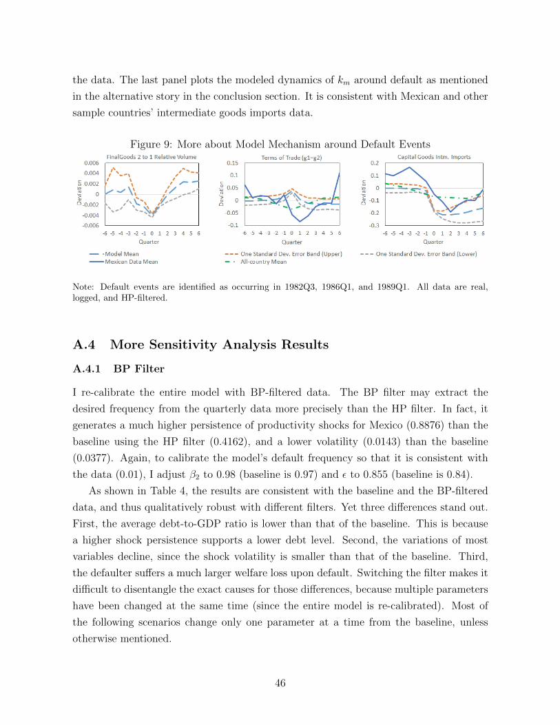
the data. The last panel plots the modeled dynamics of km around default as mentioned
in the alternative story in the conclusion section. It is consistent with Mexican and other
sample countries’ intermediate goods imports data.
Figure 9: More about Model Mechanism around Default Events
Note: Default events are identified as occurring in 1982Q3, 1986Q1, and 1989Q1. All data are real,logged, and HP-filtered.
A.4 More Sensitivity Analysis Results
A.4.1 BP Filter
I re-calibrate the entire model with BP-filtered data. The BP filter may extract the
desired frequency from the quarterly data more precisely than the HP filter. In fact, it
generates a much higher persistence of productivity shocks for Mexico (0.8876) than the
baseline using the HP filter (0.4162), and a lower volatility (0.0143) than the baseline
(0.0377). Again, to calibrate the model’s default frequency so that it is consistent with
the data (0.01), I adjust β2 to 0.98 (baseline is 0.97) and ε to 0.855 (baseline is 0.84).
As shown in Table 4, the results are consistent with the baseline and the BP-filtered
data, and thus qualitatively robust with different filters. Yet three differences stand out.
First, the average debt-to-GDP ratio is lower than that of the baseline. This is because
a higher shock persistence supports a lower debt level. Second, the variations of most
variables decline, since the shock volatility is smaller than that of the baseline. Third,
the defaulter suffers a much larger welfare loss upon default. Switching the filter makes it
difficult to disentangle the exact causes for those differences, because multiple parameters
have been changed at the same time (since the entire model is re-calibrated). Most of
the following scenarios change only one parameter at a time from the baseline, unless
otherwise mentioned.
46

Tab
le4:
Sen
siti
vit
yA
nal
ysi
s
Sta
tistics
HP
BP
Shock
Persistence
Intm
.Loss
Intm
.Pro
d.Share
Dat
aB
ase
lin
eD
ata
Mod
elρ
=0.
2ρ
=0.
6ε
=0.
81
ε=
0.87
α3
=0.
52
α3
=0.
56
Def
ault
freq
uen
cy0.0
11
0.0
11
0.011
0.0
11
0.0
09
0.0
13
0.0
11
0.0
11
0.012
0.013
Ave
.d
ebt/
GD
Pra
tio
(%)
74.9
427.4
474.
94
26.7
728.2
826.3
333.2
721.6
229.
66
24.
68
Ave
.sp
read
s(%
)4.
35
4.5
94.
35
3.6
14.6
24.5
54.5
84.6
14.
58
4.55
Sp
read
sst
d.
dev
.(%
)4.7
12.4
44.
71
2.7
32.3
02.6
52.4
62.4
22.
56
2.64
RE
XR
std
.d
ev.
(%)
17.3
01.9
917.
30
1.7
11.8
52.1
52.3
81.6
21.
89
2.47
Ter
ms
oftr
ade
std
.d
ev.
(%)
6.2
13.8
75.
32
3.1
93.6
24.1
74.6
73.1
44.
04
4.31
Dom
.p
rod
.co
ns.
std
/GD
Pst
d.
1.2
30.9
61.
15
0.9
20.9
60.9
70.9
31.0
00.
96
0.93
Tot
alco
ns.
std
./G
DP
std
.1.1
21.0
91.
10
1.0
91.0
81.0
91.0
91.0
81.
10
1.08
Tra
de
bal
ance
std
.(%
)2.0
81.4
01.
90
1.3
31.2
91.5
31.6
31.1
61.
58
1.39
Correlation
with
GDP
Bon
dsp
read
s−
0.3
9−
0.92−
0.2
3−
0.88
−0.
94
−0.
90
−0.
95
−0.
87
−0.
91
−0.
93
Rea
lex
chan
gera
te0.5
30.5
40.
44
0.6
70.5
20.5
30.6
50.4
00.
54
0.63
Ter
ms
ofT
rad
e0.2
50.4
90.
31
0.6
70.4
70.4
80.6
00.3
40.
50
0.59
Tra
de
bal
ance
/GD
P−
0.6
5−
0.20−
0.7
4−
0.15
−0.
18
−0.
21
−0.
19
−0.
21
−0.
19
−0.
18
Tot
alex
por
ts0.2
10.8
50.
27
0.8
80.8
50.8
50.8
60.8
50.
86
0.84
Inte
rmed
iate
good
sex
por
ts0.1
80.8
50.
22
0.8
80.8
50.8
50.8
60.8
50.
86
0.84
Tot
alim
por
t0.
75
0.9
20.
87
0.9
20.9
20.9
20.9
30.9
10.
91
0.92
GD
Pvol
um
e0.
65
0.7
90.
77
0.8
10.7
90.8
10.7
50.8
40.
79
0.75
Def
ault
occ
urr
ence
−0.1
4−
0.24−
0.0
8−
0.24
−0.
24
−0.
24
−0.
25
−0.
23
−0.
25
−0.
25
Def
ault
du
rati
on−
0.39
−0.
64−
0.3
8−
0.75
−0.
62
−0.
65
−0.
69
−0.
57
−0.6
6−
0.69
Correlation
with
bond
spre
ads
Rea
lex
chan
gera
te−
0.76
−0.
78−
0.7
6−
0.8
9−
0.74
−0.
79
−0.
82
−0.
72
−0.7
8−
0.83
Ter
ms
ofT
rad
e−
0.13
−0.7
7−
0.11−
0.9
1−
0.72
−0.
77
−0.
80
−0.
71
−0.7
8−
0.82
Tra
de
bal
ance
/GD
P0.
30
0.5
00.
16
0.7
00.4
40.5
80.5
10.4
90.
50
0.50
Tot
alex
por
ts−
0.02
−0.6
3−
0.04−
0.0
5−
0.69
−0.5
4−
0.57
−0.
70
−0.
65
−0.
49
Inte
rmed
iate
good
sex
por
ts−
0.08
−0.6
5−
0.05−
0.07
−0.
71
−0.5
6−
0.5
9−
0.71
−0.
67
−0.
51
Tot
alim
por
t−
0.28
−0.9
1−
0.17−
0.87
−0.
89
−0.9
2−
0.8
9−
0.93
−0.
89
−0.
90
GD
Pvol
um
e−
0.19
−0.
52−
0.13−
0.48
−0.5
6−
0.5
1−
0.5
4−
0.5
0−
0.51
−0.4
8D
efau
ltocc
urr
ence
0.1
80.2
60.
18
0.2
70.2
50.2
60.2
60.2
60.
26
0.26
Def
ault
du
rati
on0.5
60.8
60.
56
0.9
20.8
20.8
80.8
50.8
60.
87
0.87
Upon
default
Ave
.T
OT
dev
iati
onin
aye
ar−
0.06
−0.
07−
0.06−
0.06
−0.0
8−
0.06
−0.0
9−
0.0
5−
0.07
−0.0
8A
ve.
cred
itor
’sw
elfa
red
evia
tion
(%)
n.a
.−
0.04
n.a
.−
0.04
−0.0
4−
0.04
−0.0
5−
0.0
3−
0.05
−0.0
4A
ve.
def
ault
er’s
wel
fare
dev
iati
on(%
)n
.a.
−0.
31
n.a
.−
0.50
−0.2
3−
0.44
−0.3
1−
0.3
0−
0.30
−0.3
0A
ve.
wor
ldw
elfa
red
evia
tion
(%)
n.a
.−
0.35
n.a
.−
0.54
−0.2
7−
0.48
−0.3
6−
0.3
3−
0.35
−0.3
4
Not
e:E
xce
pt
for
bon
dsp
read
s,d
ebt-
to-G
DP
rati
o,
an
dd
efau
ltocc
urr
ence
an
dd
ura
tion
,all
oth
erd
ata
inth
eta
ble
are
HP
-filt
ered
.A
lld
ata
are
inre
alte
rms
and
atqu
arte
rly
freq
uen
cy.
For
BP
filt
erm
od
elre
sult
s,β2
=0.
98,ε
=0.
855,
shock
pro
cessρ
=0.
8876
an
dσ
=0.
0143.
47

Tab
le5:
Sen
siti
vit
yA
nal
ysi
s:P
refe
rence
Sta
tistics
HP
Patience
HomeBias
Substitution
θ 1=
0.5
Data
Base
lin
eβ2
=0.
955
β2
=0.
985
g 1=g 2
θ 2=
0.56
θ 2=
0.64
θ 2=
0.5
Def
ault
freq
uen
cy0.0
11
0.0
11
0.018
0.005
0.0
07
0.0
11
0.0
12
0.0
10
Ave
.d
ebt/
GD
Pra
tio
(%)
74.
94
27.4
424.
46
31.
01
38.1
228.3
626.6
626.6
3A
ve.
spre
ads
(%)
4.35
4.5
96.
04
3.14
4.6
64.5
74.5
84.5
7S
pre
ads
std
.d
ev.
(%)
4.7
12.4
42.
48
1.85
2.0
22.5
52.5
52.5
2R
EX
Rst
d.
dev
.(%
)17.
30
1.9
92.
53
1.27
0.0
02.1
22.0
52.2
5T
erm
sof
trad
est
d.
dev
.(%
)6.2
13.8
74.
89
2.48
1.8
44.0
84.0
83.9
4D
om.
pro
d.
con
s.st
d/G
DP
std
.1.2
30.9
60.
93
0.98
1.3
90.9
60.9
40.9
8T
otal
con
s.st
d./
GD
Pst
d.
1.1
21.0
91.
10
1.02
1.1
61.0
91.0
91.0
8T
rad
eb
alan
cest
d.
(%)
2.0
81.4
01.
89
0.74
1.7
01.4
71.4
61.3
2Correlation
with
GDP
Bon
dsp
read
s−
0.39
−0.9
2−
0.9
6−
0.81
−0.
86
−0.
93
−0.9
0−
0.95
Rea
lex
chan
gera
te0.5
30.5
40.
66
0.13
−0.
38
0.5
80.5
60.5
8T
erm
sof
Tra
de
0.2
50.4
90.
63
0.10
−0.
67
0.5
30.5
30.5
3T
rad
eb
alan
ce/G
DP
−0.
65
−0.
20
−0.1
6−
0.0
4−
0.11
−0.
20
−0.1
8−
0.2
1T
otal
exp
orts
0.2
10.8
50.
84
0.91
0.9
70.8
60.8
40.8
5In
term
edia
tego
od
sex
por
ts0.1
80.8
50.
84
0.91
0.8
60.8
60.8
40.8
6T
otal
imp
ort
0.75
0.9
20.
91
0.92
0.9
00.9
30.9
00.9
5G
DP
vol
um
e0.
65
0.7
90.
72
0.88
0.9
10.7
70.7
90.7
6D
efau
ltocc
urr
ence
−0.1
4−
0.24
−0.2
6−
0.2
0−
0.23
−0.
24
−0.2
5−
0.2
3D
efau
ltd
ura
tion
−0.3
9−
0.64
−0.7
2−
0.5
0−
0.50
−0.
66
−0.6
6−
0.6
6Correlation
with
bond
spre
ads
Rea
lex
chan
gera
te−
0.7
6−
0.78
−0.8
2−
0.5
5−
0.09
−0.
78
−0.8
2−
0.7
6T
erm
sof
Tra
de
−0.1
3−
0.77
−0.8
0−
0.5
40.2
5−
0.77
−0.8
2−
0.7
3T
rad
eb
alan
ce/G
DP
0.3
00.5
00.
63
0.24
0.4
80.5
00.5
10.5
1T
otal
exp
orts
−0.0
2−
0.63
−0.2
9−
0.8
3−
0.83
−0.
62
−0.5
8−
0.5
9In
term
edia
tego
od
sex
por
ts−
0.0
8−
0.65
−0.3
2−
0.8
4−
0.94
−0.
64
−0.6
1−
0.6
1T
otal
imp
ort
−0.2
8−
0.91
−0.9
2−
0.9
2−
0.95
−0.
90
−0.9
0−
0.9
2G
DP
vol
um
e−
0.1
9−
0.52
−0.5
2−
0.5
0−
0.58
−0.
53
−0.4
8−
0.5
5D
efau
ltocc
urr
ence
0.1
80.2
60.
24
0.30
0.2
60.2
60.2
60.2
5D
efau
ltd
ura
tion
0.5
60.8
60.
84
0.86
0.8
30.8
50.8
80.8
2Upon
default
Ave
.T
OT
dev
iati
onin
aye
ar−
0.0
6−
0.07
−0.0
8−
0.0
70.0
0−
0.07
−0.0
8−
0.0
7A
ve.
cred
itor
’sw
elfa
red
evia
tion
(%)
n.a
.−
0.04
−0.0
4−
0.0
5−
0.07
−0.
04
−0.0
4−
0.0
8A
ve.
def
ault
er’s
wel
fare
dev
iati
on(%
)n
.a.
−0.
31
−0.4
1−
0.1
8−
0.23
−0.
29
−0.3
2−
0.2
7A
ve.
wor
ldw
elfa
red
evia
tion
(%)
n.a
.−
0.35
−0.4
5−
0.2
3−
0.30
−0.
33
−0.3
6−
0.3
5
Not
e:E
xce
pt
for
bon
dsp
read
s,d
ebt-
to-G
DP
rati
o,
an
dd
efau
ltocc
urr
ence
an
dd
ura
tion
,all
oth
erd
ata
inth
eta
ble
are
HP
-filt
ered
.A
lld
ata
are
inre
alte
rms
and
atqu
arte
rly
freq
uen
cy.
Forθ 1
=θ 2
=0.
5,
Ire
-cali
bra
teth
em
od
elto
hav
eρ1
=0.
8,ρ2
=0.
8,
an
dβ2
=0.
98.
48

A.4.2 Shock Persistence
The next two columns of Table 4 report the results for shocks with lower persistence
(ρ = 0.2) and higher persistence (ρ = 0.6) than the baseline (ρ = 0.4162). Comparing
the three scenarios, I find that most variables have small changes that are monotonic
with the change in shock persistence. Some more significant changes occur to the average
debt-to-GDP ratio, and the defaulter’s welfare losses.
First, lower shock persistence allows a country to get back on track faster after an
adverse productivity shock and thus to maintain a higher average debt level. Second,
lower shock persistence also leads to a smaller welfare loss for the defaulting country.
These changes are reversed in the case of higher shock persistence.
A.4.3 Patience
The discount factor β2 = 0.97 in the baseline is much higher than the value commonly
used in the sovereign default literature. For instance, the discount factors in Aguiar and
Gopinath (2006), Arellano (2008), Yue (2010), and Mendoza and Yue (2012) are all below
0.953. However, it is lower than the typical value in the real business cycle literature. Here
I analyze how the results differ with the value of the discount factor. A lower discount
factor of 0.955 and a higher one of 0.985 are used to compare the results with the baseline’s
0.97 in Table 5. The variable values change monotonically with the discount factor.
As expected, a government that care less about the future brings more frequent de-
faults, a lower average debt-to-GDP ratio, and a higher average bond spread. Meanwhile,
less patience also generates more volatility in total consumption and trade over business
cycles, moving the model results closer to the data. The resulting terms of trade and real
exchange rates also fluctuate more in correlation with GDP and bond spreads. In addition,
the borrower registers a much larger post-default welfare loss than in the baseline.
A.5 Data Sources
GDP value (in USD) and volume (in index), trade value (in USD) and volume (in index),
trade as a share of GDP, net barter terms of trade, real exchange rate, and consumption
are from the IMF and the World Bank. Trade volume index is calculated as the ratio of the
export value index to the corresponding unit value index. Real Effective Exchange Rates
for Mexico come from FRED, maintained by the Federal Reverse Bank of St. Louis.
Mexico’s domestic capital stock is calculated by the author from combined data from
FRED and the IMF.
49

I use Mexico’s treasury bill rates from the IMF as its sovereign bond interest rates,
and calculate the bond spreads with the U.S. government bond interest rates (FRED).
Mexico’s external public debt is from the combined sources of Mexico’s Secretary of
Finance and Public Credit and the IMF.
The frequency of defaults over the long term is calculated with information from
Reinhart (2010). Sample default episodes are based on Reinhart (2010), Mendoza and Yue
(2012), and the treatment dates from the Paris Club. Slight date adjustments according
to GDP fluctuations are made with regard to the Paris Club dates to reflect delayed
treatments after defaults. The results are not sensitive to the default date adjustments.
The annual data for the intermediate goods exports of multiple countries (see Table 6)
come from the World Bank (WITS). The quarterly data for Mexico’s intermediate goods
exports are from Mexico’s National Institute of Statistics and Geography (INEGI). They
are also cross-checked with Mexico’s annual intermediate goods exports data from the
World Bank.
Mexico’s total hours worked comes from FRED, unemployment rates from the IMF,
and total employment from the combined sources of the World Bank (WDI), the IMF,
and Mexico’s INEGI. Total FDI stock in Mexico is calculated using annual data from the
OECD, U.S. Bureau of Economic Analysis (BEA), and the IMF. Furthermore, according
to the UN’s 2013 report on Foreign Direct Investment in Latin America and Caribbean,
about 4.4 jobs are created in Mexico for every 1 million USD invested from abroad during
the period 2003-2013. Using this number, I impute Mexico’s FDI related employment
according to its FDI stock data. Hence, Mexico’s domestic sector employment is its
total employment minus its FDI employment. In calibration, the data for labor share in
production is from the OECD. Canadian employment is from Statistics Canada.
For the empirical regressions, the data for Mexican and U.S. inputs to Canadian
manufacturing industries are obtained from World Input-Output Database. The data for
Canadian manufacturing output by industry is from Statistics Canada.
50

Tab
le6:
Def
ault
Eve
nts
and
Dat
aA
vailab
ilit
y
Country
Event
Available
Data
Arg
enti
na
1982
TO
T,
GD
Pval.,
GD
Pvol.,
Exp
.val.,
Exp
.vol.
,E
xp
/G
DP
,Im
p.
val.,
Imp
.vol.,
Imp
/G
DP
,In
tm.
imp
.val.
2002
TO
T,
GD
Pval.,
GD
Pvol.,
Exp
.val.,
Exp
.vol.,
Exp
/G
DP
,Im
p.
val.,
Imp
.vol.,
Imp
/G
DP
,In
tm.
exp
.&
imp
.val.,
Intm
.ex
p.
vol.,
Intm
.ex
p./
GD
PB
razi
l1983
RE
XR
,T
OT
,G
DP
val.,
GD
Pvol.,
Exp
.val.
,E
xp
.vol.,
Exp
/G
DP
,Im
p.
val.,
Imp
.vol.,
Imp
/G
DP
Ch
ile
1983
RE
XR
,T
OT
,G
DP
val.,
GD
Pvol.,
Exp
.val.,
Exp
.vol.,
Exp
/G
DP
,Im
p.
val.,
Imp
.vol.,
Imp
/G
DP
Cro
ati
a1992
RE
XR
,G
DP
vol.,
Exp
.val.,
Imp
.val.,
Intm
.im
p.
val.
Dom
.R
ep.
1982
RE
XR
,T
OT
,G
DP
val.,
GD
Pvol.,
Exp
.val.,
Exp
.vol.,
Exp
/G
DP
,Im
p.
val.,
Imp
.vol.,
Imp
/G
DP
1993
RE
XR
,T
OT
,G
DP
val.,
GD
Pvol.,
Exp
.val.,
Exp
.vol.,
Exp
/G
DP
,Im
p.
val.,
Imp
.vol.,
Imp
/G
DP
2003
RE
XR
,T
OT
,G
DP
val.,
GD
Pvol.,
Exp
.val.,
Exp
.vol.,
Exp
/G
DP
,Im
p.
val.,
Imp
.vol.,
Imp
/G
DP
Ecu
ad
or
1999
RE
XR
,T
OT
,G
DP
val.,
GD
Pvol.,
Exp
.val.,
Exp
.vol.,
Exp
/G
DP
,Im
p.
val.,
Imp
.vol.,
Imp
/G
DP
,In
tm.
exp
.&
imp
.val.,
Intm
.ex
p.
vol.,
Intm
.ex
p./
GD
PE
gyp
t1984
TO
T,
GD
Pval.,
GD
Pvol.,
Exp
.val.,
Exp
.vol.,
Exp
/G
DP
,Im
p.
val.,
Imp
.vol.,
Imp
/G
DP
Gre
ece
2009
RE
XR
,T
OT
,G
DP
val.,
GD
Pvol.,
Exp
.val.,
Exp
.vol.,
Exp
/G
DP
,Im
p.
val.,
Imp
.vol.,
Imp
/G
DP
,In
tm.
exp
.&
imp
.val.,
Intm
.ex
p.
vol.,
Intm
.ex
p./
GD
PIc
elan
d2008
RE
XR
,T
OT
,G
DP
val.,
GD
Pvol.,
Exp
.val.,
Exp
.vol.,
Exp
/G
DP
,Im
p.
val.,
Imp
.vol.
,Im
p/G
DP
,In
tm.
exp
.&
imp
.val.,
Intm
.ex
p.
vol.,
Intm
.ex
p./
GD
PIn
don
esia
1998
TO
T,
GD
Pval.,
GD
Pvol.,
Exp
.val.,
Exp
.vol.,
Exp
/G
DP
,Im
p.
val.,
Imp
.vol.,
Imp
/G
DP
,In
tm.
exp
.&
imp
.val.,
Intm
.ex
p.
vol.,
Intm
.ex
p./
GD
PM
exic
o1982
RE
XR
,T
OT
,G
DP
val.,
GD
Pvol.
,E
xp
.val.,
Exp
.vol.,
Exp
/G
DP
,Im
p.
val.,
Imp
.vol.,
Imp
/G
DP
,In
tm.
exp
.val.,
Intm
.ex
p.
vol.,
Intm
.ex
p./
GD
P1986
RE
XR
,T
OT
,G
DP
val.,
GD
Pvol.,
Exp
.val.,
Exp
.vol.,
Exp
/G
DP
,Im
p.
val.,
Imp
.vol.,
Imp
/G
DP
,In
tm.
exp
.val.,
Intm
.ex
p.
vol.,
Intm
.ex
p./
GD
P1989
RE
XR
,T
OT
,G
DP
val.,
GD
Pvol.,
Exp
.val.,
Exp
.vol.,
Exp
/G
DP
,Im
p.
val.,
Imp
.vol.,
Imp
/G
DP
,In
tm.
exp
.val.,
Intm
.ex
p.
vol.,
Intm
.ex
p./
GD
PM
old
ova
2002
RE
XR
,T
OT
,G
DP
val.,
Exp
.val.
,E
xp
.vol.,
Exp
/G
DP
,Im
p.
val.,
Imp
.vol.,
Imp
/G
DP
,In
tm.
exp
.&
imp
.val.,
Intm
.ex
p.
vol.,
Intm
.ex
p./
GD
PM
oro
cco
1983
TO
T,
GD
Pval.
,G
DP
vol.,
Exp
.val.,
Exp
.vol.,
Exp
/G
DP
,Im
p.
val.,
Imp
.vol.,
Imp
/G
DP
1986
TO
T,
GD
Pval.,
GD
Pvol.,
Exp
.val.,
Exp
.vol.,
Exp
/G
DP
,Im
p.
val.,
Imp
.vol.,
Imp
/G
DP
Nig
eria
1983
RE
XR
,T
OT
,G
DP
val.,
GD
Pvol.,
Exp
.val.
,E
xp
.vol.,
Exp
/G
DP
,Im
p.
val.,
Imp
.vol.,
Imp
/G
DP
1986
RE
XR
,T
OT
,G
DP
val.,
GD
Pvol.,
Exp
.val.,
Exp
.vol.,
Exp
/G
DP
,Im
p.
val.,
Imp
.vol.,
Imp
/G
DP
1992
RE
XR
,T
OT
,G
DP
val.,
GD
Pvol.,
Exp
.val.,
Exp
.vol.,
Exp
/G
DP
,Im
p.
val.,
Imp
.vol.,
Imp
/G
DP
2001
RE
XR
,T
OT
,G
DP
val.,
GD
Pvol.,
Exp
.val.,
Exp
.vol.,
Exp
/G
DP
,Im
p.
val.,
Imp
.vol.,
Imp
/G
DP
Pakis
tan
1998
RE
XR
,T
OT
,G
DP
val.,
GD
Pvol.,
Exp.
val.,
Exp
.vol.,
Exp
/G
DP
,Im
p.
val.,
Imp
.vol.,
Imp
/G
DP
Para
gu
ay
1986
RE
XR
,T
OT
,G
DP
val.,
GD
Pvol.,
Exp
.vol.,
Imp
.vol.
2003
RE
XR
,T
OT
,G
DP
val.,
GD
Pvol.,
Exp
.val.,
Exp
.vol.,
Exp
/G
DP
,Im
p.
val.,
Imp
.vol.,
Imp
/G
DP
Per
u1983
TO
T,
GD
Pval.,
GD
Pvol.,
Exp
.val.,
Exp
.vol.,
Exp
/G
DP
,Im
p.
val.,
Imp
.vol.,
Imp
/G
DP
Ph
ilip
ines
1983
RE
XR
,T
OT
,G
DP
val.,
GD
Pvol.,
Exp
.val.,
Exp
.vol.,
Exp
/G
DP
,Im
p.
val.,
Imp
.vol.,
Imp
/G
DP
Rom
an
ia1981
GD
Pval.,
GD
Pvol.
1986
GD
Pval.,
GD
Pvol.
Ru
ssia
1998
RE
XR
,G
DP
val.,
GD
Pvol.,
Exp
.val.,
Exp
/G
DP
,Im
p.
val.,
Imp
/G
DP
,In
tm.
exp
.&
imp
.val.,
Intm
.ex
p.
vol.,
Intm
.ex
p./
GD
PS
.A
fric
a1985
RE
XR
,T
OT
,G
DP
val.
,G
DP
vol.,
Exp
.val.,
Exp
.vol.,
Exp
/G
DP
,Im
p.
val.,
Imp
.vol.,
Imp
/G
DP
1989
RE
XR
,T
OT
,G
DP
val.,
GD
Pvol.,
Exp
.val.,
Exp
.vol.,
Exp
/G
DP
,Im
p.
val.,
Imp
.vol.,
Imp
/G
DP
1993
RE
XR
,T
OT
,G
DP
val.,
GD
Pvol.,
Exp
.val.,
Exp
.vol.,
Exp
/G
DP
,Im
p.
val.,
Imp
.vol.,
Imp
/G
DP
,In
tm.
exp
.&
imp
.val.,
Intm
.ex
p.
vol.,
Intm
.ex
p./
GD
PT
hailan
d1998
TO
T,
GD
Pval.,
GD
Pvol.,
Exp
.val.,
Exp
.vol.,
Exp
/G
DP
,Im
p.
val.,
Imp
.vol.,
Imp
/G
DP
,In
tm.
exp
.&
imp
.val.,
Intm
.ex
p.
vol.,
Intm
.ex
p./
GD
PT
urk
ey1978
GD
Pval.,
GD
Pvol.,
Exp
/G
DP
,Im
p/G
DP
1982
TO
T,
GD
Pval.,
GD
Pvol.,
Exp
.vol.,
Exp
/G
DP
,Im
p.
vol.,
Imp
/G
DP
Intm
.im
p.
val.
2000
TO
T,
GD
Pval.,
GD
Pvol.,
Exp
.val.,
Exp
.vol.,
Exp
/G
DP
,Im
p.
val.,
Imp
.vol.,
Imp
/G
DP
Intm
.ex
p.
&im
p.
val.,
Intm
.ex
p.
vol.,
Intm
.ex
p./
GD
PU
kra
ine
1998
RE
XR
,G
DP
val.,
Exp
.val.,
Exp
.vol.,
Exp
/G
DP
,Im
p.
val.,
Imp
.vol.,
Imp
/G
DP
,In
tm.
exp
.&
imp
.val.,
Intm
.ex
p.
vol.,
Intm
.ex
p./
GD
PU
rugu
ay
1990
RE
XR
,T
OT
,G
DP
val.,
GD
Pvol.,
Exp
.val.
,E
xp
.vol.,
Exp
/G
DP
,Im
p.
val.,
Imp
.vol.,
Imp
/G
DP
2003
RE
XR
,T
OT
,G
DP
val.,
GD
Pvol.,
Exp
.val.,
Exp
.vol.,
Exp
/G
DP
,Im
p.
val.,
Imp
.vol.,
Imp
/G
DP
Intm
.ex
p.
&im
p.
val.,
Intm
.ex
p.
vol.,
Intm
.ex
p./
GD
PV
enez
uel
a1995
RE
XR
,T
OT
,G
DP
val.
,G
DP
vol.,
Exp
.val.,
Exp
.vol.,
Exp
/G
DP
,Im
p.
val.,
Imp
.vol.,
Imp
/G
DP
,In
tm.
exp
.&
imp
.val.,
Intm
.ex
p.
vol.,
Intm
.ex
p./
GD
P1998
RE
XR
,T
OT
,G
DP
val.,
GD
Pvol.,
Exp
.val.,
Exp
.vol.,
Exp
/G
DP
,Im
p.
val.,
Imp
.vol.,
Imp
/G
DP
,In
tm.
exp
.&
imp
.val.,
Intm
.ex
p.
vol.,
Intm
.ex
p./
GD
P2004
RE
XR
,T
OT
,G
DP
val.,
GD
Pvol.,
Exp
.val.,
Exp
.vol.,
Exp
/G
DP
,Im
p.
val.,
Imp
.vol.,
Imp
/G
DP
,In
tm.
exp
.&
imp
.val.,
Intm
.ex
p.
vol.,
Intm
.ex
p./
GD
PV
ietn
am
1993
GD
Pval.,
GD
Pvol.,
Exp
.val.,
Imp
.val.
Note
:In
term
edia
tegood
sex
port
valu
e,volu
me,
an
dsh
are
of
GD
Pare
als
oavailab
lefo
rB
razi
lan
dP
eru
sin
ce1988,
aft
erth
eir
sover
eign
def
au
lts.
Th
ed
ati
ng
of
exte
rnal
deb
td
efau
lts
com
esm
ain
lyfr
om
Men
doza
an
dY
ue
(2012)
an
dR
ein
hart
(2010).
Oth
erd
ati
ng
sou
rces
for
cross
-ch
eckin
gin
clu
de
Laev
enan
dV
ale
nci
a(2
008)
an
dth
eP
ari
sC
lub
data
.
51
Related Documents