A Systematic Approach to Modeling Organic Rankine Cycle ...

A Systematic Approach to Modeling Organic Rankine Cycle Systemsfor Global Optimization

Vathna Am1, Jonathan Currie2 and David I. Wilson3

Abstract— The demand for organic Rankine cycle (ORC)systems to be efficient and economically competitive drivesthe need for a reliable and robust modeling approach thatis suitable for optimization. However existing commercialsimulation software is not typically tailored for optimizationand they generally cannot guarantee global optimum. Thispaper proposes a modeling approach to approximate a rigoroussimulation model that is suitable for global optimization.This involves a combination of regression and thermodynamicanalysis, in addition to integer programming techniques. Threedifferent solvers, COBYLA, SCIP, and BARON are used tooptimize the ORC model and are compared against each otherto demonstrate the prospect of achieving the global optimumusing this approach. In addition, this paper also presents atechnique to improve the model accuracy by using a piecewisefit to approximate the output characteristic of the ORC unitoperations.

I. I NTRODUCTION

With the inevitability of the world’s non-renewable re-sources becoming scarcer and the progressive pressure for thepower generation sector to reduce greenhouse gases emissionand pollutants, there has been a massive growth in renewablepower generation technologies. Geothermal energy is oneexample of a reliable source of sustainable energy. As of2010, there are 24 countries that have used geothermalenergy for electricity generation [1]. Of all the geothermalpower plants (GPP), organic Rankine cycle (ORC) powerplants are the most common type of geothermal power plantsin the world with 203 units in operation as of December2014, constituting to over 35% of all geothermal units [2].

Given the large number of ORC systems around the worldand the potential for more to be installed due to the relativelyabundant low-temperature geothermal resources, there is aconsiderable amount of literature on ORC modeling andoptimization. Often these ORC plants are simulated usingthe sequential modular approach, via a standard modelingsoftware such as Aspen Plus [3] or GateCycle [4], andthen are subsequently optimized using heuristic methods orsophisticated algorithms [5], [6].

However, one major concern with using this approach liesin the robustness and efficiency of the model when it is usedin optimization problems. Therefore, this paper will discussthe limitations of sequential modular models and propose

1School of Engineering, Computer & Mathematical Sciences, Auck-land University of Technology, Auckland, New Zealand; e-mail:[email protected]

2School of Engineering, Computer & Mathematical Sciences, AucklandUniversity of Technology, Auckland, New Zealand

3Industrial Information & Control Centre, Auckland University of Tech-nology, Auckland, New Zealand

a modeling approach for ORC systems that is intended forefficient global optimization.

II. SEQUENTIAL MODULAR MODEL AND

EQUATION-ORIENTED MODEL

Traditionally, GPPs are often modeled using the sequentialmodular (SM) approach where unit operation modules (orfunctions) are linked together in the flow order through theplant. The output of each module is calculated from theoutput of the previous module in the flowsheet; therefore, thestream information, i.e. mass flows, temperatures, enthalpies,etc., will propagate from the beginning of the plant’s processthrough to the end of the flowsheet.

However, there are some key limitations to using theSM approach, especially when dealing with optimizationproblems. Many of the derivative optimization solvers, likefmincon(MATLAB’s solver) [7] or IPOPT [8], that requirethe first and/or second derivatives of the objective functionand constraints, will struggle to find accurate derivativesfromSM models due to complex thermodynamics and/or internalmodel iterations. Consequently, the derivatives are approxi-mated using finite differences leading to various optimizationproblems such as convergence issues and long computationtimes [9]. Furthermore, it is recognized that optimizationproblems are solved more accurately and efficiently if theanalytical derivative functions are provided, [10], [11]. Inaddition, solvers that are compatible with the SM modelstructure cannot guarantee that the optimum found is theglobal optimum, which might be a disadvantage in today’scompetitive market.

An alternative method is to use the equation-oriented(EO) approach, where systems are represented as a set ofequations that are solved simultaneously. In contrast, to theSM approach, EO approach allows standard optimizationproblems to be formulated relatively efficiently from themodel structure, and the mass and energy balance equationsare solved simultaneously with the optimization problem[12]. In addition, provided that if all the equations are alge-braic and analytically differentiable, some global optimizers(white-box optimizers) can exploit this algebraic structureand analytically calculate the required derivatives for opti-mization. This means that the numerical issues discussedabove can be bypassed or reduced. Thus, this paper aimsto demonstrate how an ORC system can be modeled andoptimized using an algebraic EO approach and using white-box global solvers, namely SCIP [13] and BARON [14],to deterministically find the global optimum of the plant.

Furthermore, the results will be compared with a black-box optimizer, namely COBYLA [15] (supplied by NLopt[16]), that cannot guarantee global optimality to highlightthe difference between the two optimization techniques. Thenovelty of this research is the application of the proposedmodeling framework to an ORC system to address the issuesassociated with the conventional SM optimization approachand to provide an efficient model that is tailored for globaloptimization.

III. M ODELING AN ORC SYSTEM

This paper illustrates the proposed modeling approachusing a simple four-unit-operation ORC system. Fig. 1 showsthe process flow diagram (PFD) of the ORC system, whichconsists of a cycle including a turbine, condenser, feed pump,and an evaporator. The topology of this ORC system has beenanalyzed extensively in many academic papers [17]–[19] andin many standard thermodynamic textbooks such as [2], [20].

A. Model Description

The specific ORC system described in [19] was usedto demonstrate the proposed modeling approach with plantparameters labeled in Fig. 1. Since this research focusesmainly on the modeling and optimization aspect of an ORCsystem, and not the effect of different working fluids, onlyR227ea (1, 1, 1, 2, 3, 3, 3-Heptafluoropropane) was used dueto its favorable thermodynamic properties.

In addition, the ORC system was assumed as a steady-state and steady-flow process; whereby changes in kineticand potential energy were neglected, and losses induced byfriction were neglected. The thermodynamic and transportproperties of the brine were considered to be the sameas water; chemical substances and non-condensible gaseswere neglected. Furthermore, the pressure drops across heatexchangers and pipelines were neglected.

B. High Fidelity SM Model

The high fidelity SM model in this research was con-structed using JSteam MATLAB Toolbox v1.70 [21]. Theconstruction of the model used unit operation function calls

Fig. 1. The process flow diagram of a basic organic Rankine cycle system.

and the current REFPROP (version 9.1) thermodynamicpackage [22], which were considered as the “gold standard”for the purposes of this study.

As previously mentioned, these high fidelity SM modelsare not tailored for optimization. Therefore, this model wasnot built to be optimized but instead was used to validatethe approximate EO model since it provides a very accuraterepresentation of the ORC system. This is an importantpart of this proposed modeling framework, as it will showthe reliability and accuracy of the approximate EO modelto the original system. Once the model is constructed andsolved using a nonlinear system solver (such asfsolve inMATLAB), it can be used as initial guess for the optimizationproblem discussed in Section III-C. Since different initial-ization values can result in different optimization times andsolutions, it is important that a feasible initial guess is usedfor the optimization problem. Therefore, for this research, theinitialization values were taken from the base case scenario[19] that was solved in the SM model to minimize the issuesassociated with a poor initial guess.

In order to keep this paper concise, the construction of thismodel will not be discussed but a similar system is detailedin the tutorial section of the JSteam software, [21].

C. Approximate EO Model

As mentioned in Section II, in order to utilize SCIP andBARON solvers, an algebraic description of the ORC modelis required. The task of constructing the EO model of anORC systems amounts to deriving a set of deterministicalgebraic equations describing the process of the system andapproximating the output characteristic of the unit operationsusing regression and thermodynamic analysis. The followingsubsections will discuss how this model was constructed andthe compromise between the accuracy of the model and thecomputational complexity of the optimization problem.

1) Objective Function:For this optimization problem, theobjective function was to maximize the gross power outputof the plant, which is defined as

j = (h1 − h2)m1 (1)

whereh is the enthalpy value andm is the mass flow rateof the working fluid associated with the turbine in Fig. 1.

Note that this model is not limited to the gross poweroutput; the objective function can be the net power output,the mass flow of the working fluid, or even a weightedeconomic analysis of the plant.

2) Mass and Energy Balance:The first set of equationsis the mass and energy balance equations, which can bederived based on the first law of thermodynamics. Referringto Fig. 1, the following mass and energy balance equationsare associated with the numbers labeled on the diagram,wherem is the mass flow rate,h is the enthalpy value,Wpump

is the pump input power,Wturb is the turbine output power,

B is the brine and CW is the cooling water.

m1 − m2 = 0

m2 − m3 = 0

m3 − m4 = 0

m4 − m1 = 0

(2)

m1h1 − Wturb − m2h2 = 0

mCWinhCWin + m2h2 − mCWouthCWout − m3h3 = 0

m3h3 + Wpump− m4h4 = 0

mBinhBin + m4h4 − mBouthBout − m1h1 = 0

(3)

From the fixed parameters mentioned in Section III-A,the following constants were calculated using REFPROP:mBinhBin is 30144 kJ/kg,mBouthBout is 19133kJ/kg,hCWin is29.288kJ/kg,hCWout is 62.832kJ/kg. Note that while there isenough information to calculateh1, it was intentionally keptas a decision variable in order to show how the turbine unitoperation can be approximated using this modeling approach(see Section III-C.4). All the other variables in (2) and (3)aredecision variables and will be calculated by the optimizer.

3) Operational Constraints:In addition to the mass andenergy balance equations, there are operational constraintsto consider. These are subcooling requirements, the pressuredrop across heat exchangers, heat loss, etc. However, incompliance with [19] specifications and assuming that state3 can operate between 283 K and the saturated temperatureat 0.6 MPa, only the state of the working fluid entering thepump was of concern for this example, which needs to begreater or equal to 283 K.

Equation (4)h3 ≥ hf@283 K (4)

ensures that state 3 will always be greater or equal to theenthalpy value at saturated temperature of 283 K, which canbe calculated directly using REFPROP.

Whereas Equation (5)

h3 ≤ 162.362P30.301 + 100.620 (5)

ensures that state 3 will always be lower or equal to theenthalpy value at saturated liquid pressure ranging from 0.1to 0.6 MPa, whereP3 is the pressure at state 3. The righthand side of (5) was derived using a curve fitting tool,optifit[21], that fitted a curve to a set of saturated liquid enthalpyvalues ranging from 0.1 to 0.6 MPa, as shown in Fig. 2. Inthis case, the fitting model was a power function.

4) Unit Operation Approximations:Since the rigorousunit operation functions cannot be used in this EO model,the two expressions, namelyWturb andWpump, in (3) need tobe approximated as a function of enthalpy and/or pressure,hence the name approximate EO model.

The pump input power is defined in (6), where∆hpumpisen is

the isentropic pump work,ηpump is the isentropic efficiencyand m3 is the mass flow rate. Since we assume that thereare no pressure drops across the heat exchangers, i.e.P3 =P2 ∈ [0.1, 0.6] MPa andP4 = P1 = 1 MPa, and knowing thatthe quality of the working fluid will always be 0 across the

190

200

210

220

230

Sat

urat

ed L

iqui

dE

ntha

lpy

[kJ/

kg] REFPROP Values

Regressed Fit

0.1 0.2 0.3 0.4 0.5 0.6Pressure [MPa]

-0.05

0

0.05

|Err

or|

Fig. 2. Regressed fit for approximating the saturated liquidenthalpy valueas a function of pressure.

pump, a set of isentropic pump work values can be calculatedat various input pressures. The correlation between isentropicpump work and the inlet pressure can then be approximatedvia regression analysis, as shown in Fig. 3. The fitting modelthat was used to approximate the isentropic pump work wasa quadratic polynomial curve. As a result, the pump inputpower now becomes

Wpump =∆h

pumpisen m3

ηpump, (6)

where

∆hpumpisen = −0.271P3

2 − 0.389P3 + 0.626. (7)

A similar approach can also be applied to the turbineoutput power; however, there are now two independentvariables, namely the inlet enthalpy and the outlet pressure.Equation (9) defines the turbine output power, where∆hturb

isenis the isentropic turbine work,ηturb is the isentropic efficiencyand m1 is the mass flow rate. Assuming that the inlettemperature can vary between 383 K and the saturated vaportemperature at 1 MPa, and the outlet pressure can varybetween 0.1 to 0.6 MPa, a set of isentropic turbine workvalues can be calculated, as shown by the black dots inFig. 4. Since there are no explicit temperature terms in (3),

0.3

0.4

0.5

Isen

trop

ic P

ump

Wor

k [k

J/kg

] REFPROP ValuesRegressed Fit

0.1 0.2 0.3 0.4 0.5 0.6Pressure [MPa]

-2-101

|Err

or|

10-3

Fig. 3. Regressed fit for approximating the isentropic pump work as afunction of the inlet pressure.

Fig. 4. Regressed fit for approximating the isentropic turbine work as afunction of the inlet enthalpy and outlet pressure. (See also Fig. 5.)

the respective inlet enthalpy values were calculated for theinlet temperatures. Using a surface fitting tool, a correlationbetween the isentropic turbine work, the inlet enthalpy, andthe outlet pressure can be approximated as a quadraticpolynomial surface,

∆hturbisen= 76.439P3

2 − 0.203P3h1

− 23.942P3 + 0.151h1 − 16.436.(8)

So the turbine output power is now given by

Wturb = ∆hturbisenηturbm1. (9)

5) Bounds: In order to constrain the search region anddecrease the execution time, all the decision variables needto be bounded within a sensible range. For this particularoptimization problem, these bounds corresponded to: 1 to100 kg/s form; 1 to 500 kg/s formCWin ; 0.1 to 0.6 MPa forP3; 1 to 1000 kJ/kg forh; andhg@1MPa to h@363 K, 1 MPafor h1.Once all the bounds, constraints and unit operation approxi-mations have been established, the optimization problem canbe constructed, which should follow the general nonlinearprogramming format.

6) EO Model Validation: In order to ensure that theapproximate model is an accurate representation of theoriginal ORC system, the optimized results were substitutedinto the high fidelity model (discussed in Section III-B). Thisvalidates that all our approximations are within reasonabletolerance and that the optimum results have not violatedany thermodynamic laws or have not deviated too muchfrom the actual thermodynamic properties. Table I, underthe Quadratic Surface Fit column, shows the relative errorsbetween the SM and EO models, and the average time ittook for each respective optimizer to solve the optimizationproblem. In addition, Table I also shows the relative errorsbetween the SM and EO models where a piecewise fit wasused to approximate the turbine output power, instead of aquadratic polynomial surface fit. The rationale behind thisalternative approach will be discussed in Section IV.

The discrepancies between the high fidelity SM model andthe approximate EO model for all the solvers are reasonable,with the highest error being only 2.08%, thus indicates that

TABLE I

THE RELATIVE ERROR[%] BETWEEN THE APPROXIMATEEO MODEL

AND THE HIGH FIDELITY SM MODEL.

Quadratic Surface Fit Piecewise FitParameter COBYLA SCIP BARON SCIP BARONP3 0.00 0.00 0.00 0.00 0.00h1 0.00 0.00 0.00 0.00 0.00h2 0.09 0.06 0.06 0.01 0.01h3 0.00 0.00 0.00 0.00 0.00h4 0.00 0.00 0.00 0.00 0.00Turbine Power 1.99 1.53 1.53 0.26 0.26Pump Power 0.12 0.12 0.12 0.12 0.12Cooler Duty 0.20 0.16 0.16 0.03 0.03Heater Duty 0.00 0.00 0.00 0.00 0.00Working Fluid 0.00 0.00 0.00 0.00 0.00Cooling Water 0.20 0.16 0.16 0.03 0.03Thermal Efficiency 2.08 1.61 1.61 0.26 0.27Solver Time [s] 5.53 14.61 0.91 20.67 1.08

the approximate model is a fairly sensible representation ofthe original ORC system. However, it is possible to furtherimprove the accuracy of the ORC model and, in some cases,reduce the complexity (order) of the fitted function by usinga piecewise fit instead of a single surface fit.

IV. PIECEWISE FIT APPROXIMATION

From just visually inspecting the surface regression inFig. 4, there are regions that the surface fit overestimates theisentropic turbine work, which can lead to large discrepanciesif the plant were to operate in those regions. An alternativemethod is to use a piecewise fit to approximate the isentropicturbine work, as shown in Fig. 5. This allows for a moreaccurate fit and also could conceivably reduce the complexityof the fitting model. The aim here is to get a fit that hasthe lowest order (degree) possible without sacrificing theaccuracy of the model. Thus, in this research, we havedeveloped an algorithm that automatically optimizes theposition of the breaks (the location where the surfaces arejoined together, i.e. the solid lines in Fig. 5) in order tominimize the sum squared error (SSE) for a given numberof breaks.

Just visually comparing the two figures, there is an obvious

Fig. 5. Regressed fit for approximating the isentropic turbine work as afunction of the inlet enthalpy and outlet pressure, using a piecewise fit. Thesolid lines indicate the breaks between two adjacent functions.

accuracy improvement in using a piecewise fit. For thisparticular case, there are three breaks and four quadraticpolynomial surface fits, which constituted to an SSE of42.32, whereas with a single quadratic polynomial surfacefitting model, the SSE was 1835.2. Note that the color axesof the error plot in Fig. 5 are deliberately set the same asfor Fig. 4 to highlight the significant improvement in theaccuracy of the turbine model.

Mathematically, the isentropic turbine work now becomes

∆hturbisen=

∆hpwisen1

, 0.10 ≤ P3 ≤ 0.17∆h

pwisen2, 0.17 < P3 ≤ 0.26

∆hpwisen3, 0.26 < P3 ≤ 0.39

∆hpwisen4, 0.39 < P3 ≤ 0.60

(10)

where each sub-function represents the mathematical expres-sion for each fitted surface. For example

∆hpwisen1

= 373.431P32 − 0.203P3h1

− 130.973P3 + 0.151h1 − 7.204

∆hpwisen2

= 153.721P32 − 0.203P3h1

− 57.527P3 + 0.151h1 − 13.342

∆hpwisen3

= 67.274P32 − 0.203P3h1

− 12.476P3 + 0.151h1 − 19.212

∆hpwisen4

= 31.328P32 − 0.203P3h1

+ 15.806P3 + 0.151h1 − 24.775

(11)

In order to incorporate the piecewise fit into the optimizationproblem, abinary variable is added to each piecewise sub-function. However it is inefficient to multiply a binaryvariable with another variable because it introduces extranonlinearity into the optimization problem. Therefore, toget around this, a modified integer programming techniquefrom AIMMS modeling guide was implemented (in Section7.7) [23] and applied it to this problem. This is done byintroducing a new variabley and equate it to the productyi = ∆h

pwisenibi, wherebi is the binary variable. To enforceyi

to take the value of∆hpwiseni

bi, the following linear constraintsneed to be added for each of the sub-function:

yi ≤ uibi

yi ≤ ∆hpwiseni +M(1− bi)

yi ≥ ∆hpwiseni −M(1− bi)

yi ≥ libi

(12)

where ui ∈ {35.03, 27.58, 20.90, 14.49} and li ∈{23.28, 17.29, 11.87, 6.63} are the sensible upper and lowerbounds of∆h

pwiseni , and M is the big-M constant that is

equal to 100ui for this particular optimization problem.Consequently, the turbine output power now becomes

Wturb = ηturbm1

4∑

i=1

yi. (13)

In addition, respective binary variables need to be added toP3 as well so that they can restrict the pressure value to

comply with the conditions of the piecewise function in (10).

P3 ≥ 0.10b1 + 0.17b2 + 0.26b3 + 0.39b4

P3 ≤ 0.17b1 + 0.26b2 + 0.39b3 + 0.60b4(14)

Since only one sub-function can be selected, this can beenforced as follows

b1 + b2 + b3 + b4 + b5 = 1, bi ∈ {0, 1} (15)

Consequently, the overall accuracy of the approximate EOmodel has increased significantly and has reduced the dis-crepancies between SM model and the EO model to nomore than 0.3%, as shown in Table I. However, since thereare now more variables and constraints in this proposedformulation, it is reasonable to result in a longer optimizationtime for both SCIP and BARON. However, while this canbe viewed as a disadvantage, in some cases the differenceis rather small, namely BARON, and does not outweighthe significant improvement in the accuracy of the ORCmodel that this approach offers. Note that the optimizerCOBYLA cannot be used on this problem, as it cannot solveinteger programming problems, illustrating a limitation insome conventional black-box optimization schemes.

V. RESULTS

The approximate EO model was optimized using threedifferent solvers, namely one black-box solver (COBYLA)and two white-box solvers (SCIP and BARON). The opti-mized results were validated/solved in the SM model andthen compared to each other, as shown in Table II.

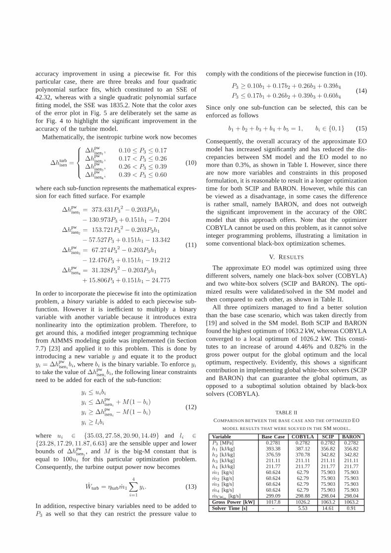
All three optimizers managed to find a better solutionthan the base case scenario, which was taken directly from[19] and solved in the SM model. Both SCIP and BARONfound the highest optimum of 1063.2 kW, whereas COBYLAconverged to a local optimum of 1026.2 kW. This consti-tutes to an increase of around 4.46% and 0.82% in thegross power output for the global optimum and the localoptimum, respectively. Evidently, this shows a significantcontribution in implementing global white-box solvers (SCIPand BARON) that can guarantee the global optimum, asopposed to a suboptimal solution obtained by black-boxsolvers (COBYLA).

TABLE II

COMPARISON BETWEEN THE BASE CASE AND THE OPTIMIZEDEO

MODEL RESULTS THAT WERE SOLVED IN THESM MODEL.

Variable Base Case COBYLA SCIP BARONP3 [MPa] 0.2781 0.2782 0.2782 0.2782h1 [kJ/kg] 393.38 387.12 356.82 356.82h2 [kJ/kg] 376.59 370.78 342.82 342.82h3 [kJ/kg] 211.11 211.11 211.11 211.11h4 [kJ/kg] 211.77 211.77 211.77 211.77m1 [kg/s] 60.624 62.79 75.903 75.903m2 [kg/s] 60.624 62.79 75.903 75.903m3 [kg/s] 60.624 62.79 75.903 75.903m4 [kg/s] 60.624 62.79 75.903 75.903mCWin [kg/s] 299.09 298.88 298.04 298.04Gross Power [kW] 1017.8 1026.2 1063.2 1063.2Solver Time [s] - 5.53 14.61 0.91

While the proposed ORC system could be solved usingbuilt-in tools in commercial software, such as sequentialquadratic programming (SQP) method in Aspen Plus, theseconventional black-box SM (flowsheet) optimization frame-works require the derivatives of the objective function andconstraints that are generally hard to obtain accurately dueto the use of complex external thermodynamic packages andrigorous unit operation modules. Consequently, this can leadto inefficient optimization and convergence issues if finitedifference is used to approximate the derivatives, especiallyfor large-scale and complex systems [11]. In addition, SMoptimization requires the entire flowsheet to be solved re-peated, which can be significantly slower and problematicto the optimization if the flowsheet fails to converge. Forthis example, it took both COBYLA andfminconrelativelylonger to optimize the SM model (around 7.25s and 6.51s,respectively) than to optimize the EO model (around 5.53sand 1.70s, respectively). Furthermore, it is important to notethat while both COBYLA andfmincondid manage to findthe global optimum of 1063.2 kW using the SM approachfor this ORC system, this SM model is only restricted toblack-box solvers and cannot assure global optimality.

VI. CONCLUSION

This paper has detailed a modeling approach for ORCsystems that is tailored to two advanced white-box globaloptimization solvers which can deterministically find theglobal optimum. The paper has demonstrated that both modelaccuracy and global optimum can be achieved by carefullyapproximating the output characteristics of the ORC unitoperations using reasonable regression and thermodynamicanalysis. The approximate EO model was optimized usingthree optimizers and then validated against a high fidelitymodel that was built using the JSteam modeling framework.As expected both SCIP and BARON found the globaloptimum, while COBYLA found a local optimum. Usingthe proposed approach to model an ORC system allowedfor exact derivatives to be calculated, which aided in theaccuracy of white-box optimizers in locating the globalsolution. In addition, the paper has shown that by using apiecewise fit, instead of a single fit function, a more accuratemodel approximation can be achieved without significantlycompromising on the performance of the solver.

ACKNOWLEDGMENT

Financial support to this project from the Industrial In-formation and Control Centre, School of Engineering, Com-puting and Mathematical Sciences, Auckland University ofTechnology, New Zealand is gratefully acknowledged.

REFERENCES

[1] R. Bertani, “Geothermal power generation in the world 2005-2010update report,”Geothermics, vol. 41, no. 2012, pp. 1–29, 2012.[Online]. Available: http://dx.doi.org/10.1016/j.geothermics.2011.10.001

[2] R. DiPippo,Geothermal Power Plants Principles, Applications, CaseStudies and Environmental Impact, 4th ed. Waltham, MA: JoeHayton: Elsevier, 2016.

[3] AspenTech, “Aspen Plus,” 2015. [Online]. Available: http://www.aspentech.com/products/engineering/aspen-plus/ [Accessed: 2015-08-24]

[4] Electric General, “GateCycle,” 2014. [Online]. Available: https://getotalplant.com/GateCycle/docs/GateCycle/index.html [Accessed:2016-08-10]

[5] H. Ghasemi, M. Paci, A. Tizzanini, and A. Mitsos, “Modelingand optimization of a binary geothermal power plant,”Energy,vol. 50, no. 1, pp. 412–428, 2013. [Online]. Available: http://dx.doi.org/10.1016/j.energy.2012.10.039

[6] A. Keceba and H. Gokgedik, “Thermodynamic evaluationof ageothermal power plant for advanced exergy analysis,”Energy,vol. 88, pp. 746–755, 2015. [Online]. Available: http://dx.doi.org/10.1016/j.energy.2015.05.094

[7] MathWorks, “fmincon,” 2016. [Online]. Available: http://au.mathworks.com/help/optim/ug/fmincon.html [Accessed: 2015-12-02]

[8] A. Wachter and L. T. Biegler, “On the implementation of an interior-point filter line-search algorithm for large-scale nonlinear program-ming,” Mathematical Programming, vol. 106, pp. 25–57, 2005.

[9] J. D. Currie, “Practical Applications of Industrial Optimization : FromHigh-Speed Embedded Controllers to Large Discrete UtilitySystems,”PhD Thesis, Dept. Elect. Eng., AUT University, 2014.

[10] C. C. Pantelides, M. Nauta, and M. Matzopoulos, “Equation-OrientedProcess Modelling Technology : Recent Advances & Current Perspec-tives,” in 5th Annual TRC-Idemitsu Workshop, Abu Dhabi, 2015.

[11] L. Biegler, Nonlinear Programming. Society for Industrial andApplied Mathematics, 2010. [Online]. Available: http://epubs.siam.org/doi/abs/10.1137/1.9780898719383

[12] R. Smith,Chemical Process Design and Integration, 2nd ed. WestSussex, United Kingdom: John Wiley & Sons Inc, 2016.

[13] T. Achterberg, “SCIP: Solving constraint integer programs,” Mathe-matical Programming Computation, vol. 1, no. 1, pp. 1–41, 2009.

[14] M. Tawarmalani and N. V. Sahinidis, “A polyhedral branch-and-cutapproach to global optimization,”Mathematical Programming, vol.103, no. 2, pp. 225–249, 2005.

[15] M. J. D. Powell,A Direct Search Optimization Method That Modelsthe Objective and Constraint Functions by Linear Interpolation.Dordrecht: Springer Netherlands, 1994, pp. 51–67.

[16] S. G. Johnson, “The NLopt nonlinear-optimization package.” [Online].Available: http://ab-initio.mit.edu/nlopt [Accessed: 2016-12-18]

[17] D. Meinel, C. Wieland, and H. Spliethoff, “Effect and comparison ofdifferent working fluids on a two-stage organic rankine cycle (ORC)concept,”Applied Thermal Engineering, vol. 63, no. 1, pp. 246–253,2014. [Online]. Available: http://dx.doi.org/10.1016/j.applthermaleng.2013.11.016

[18] D. Budisulistyo and S. Krumdieck, “Thermodynamic and economicanalysis for the pre-feasibility study of a binary geothermal powerplant,” Energy Conversion and Management, vol. 103, pp. 639–649,2015. [Online]. Available: http://linkinghub.elsevier.com/retrieve/pii/S0196890415006172

[19] A. Basaran and L. Ozgener, “Investigation of the effectof differentrefrigerants on performances of binary geothermal power plants,”Energy Conversion and Management, vol. 76, pp. 483–498, 2013.[Online]. Available: http://dx.doi.org/10.1016/j.enconman.2013.07.058

[20] Y. A. Cengel and M. A. Boles,Thermodynamics: An EngineeringApproach, 6th ed. New York: McGraw-Hill, 2008.

[21] Industrial Information & Control Centre, “Software,”2015.[Online]. Available: http://www.i2c2.aut.ac.nz/Resources/Software.html [Accessed: 2015-09-11]

[22] National Institute of Standards and Technology, “REFPROP Version9.1. NIST Standard Reference Database 23,” 2015. [Online].Available: http://www.nist.gov/srd/nist23.cfm [Accessed: 2016-02-05]

[23] J. Bisschop, “Integer Linear Programming Tricks,” inAIMMS: Opti-mization Modeling. AIMMS B.V., 2016, ch. 7, pp. 75–85.