A SYSTEM DYNAMICS APPROACH FOR STRATEGIC PLANNING …

South African Journal of Industrial Engineering Aug 2021 Vol 32(2), pp 133-149

133

A SYSTEM DYNAMICS APPROACH FOR STRATEGIC PLANNING OF CONSUMER ELECTRONICS INDUSTRY IN DEVELOPING COUNTRIES: THE CASE OF THE TELEVISION MANUFACTURING INDUSTRY IN EGYPT

M.A.A. Negmeldin1*#, M. Heshmat2 & A. Eltawil1

ARTICLE INFO

Article details Submitted by authors 1 Dec 2020 Accepted for publication 18 May 2021 Available online 31 Aug 2021

Contact details * Corresponding author [email protected]

Author affiliations 1 Department of Industrial and

Manufacturing Engineering, Egypt-Japan University of Science and Technology, Egypt

2 Department of Mechanical

Engineering, Assiut University, Egypt

# Author was enrolled for a PhD in

the Department of Industrial and Manufacturing Engineering, Egypt-Japan University of Science and Technology, Egypt

ORCID® identifiers M.A.A. Negmeldin http://orcid.org/0000-0002-5738-096X M. Heshmat http://orcid.org/0000-0003-1492-4223 A. Eltawil http://orcid.org/0000-0001-6073-8240

DOI http://dx.doi.org/10.7166/32-2-2468

ABSTRACT

In this paper, a system dynamics approach is introduced for the macro-planning of the selection of new product families in the consumer electronics industry in developing countries. A decision methodology structure is built that includes the impact factors of rapid technology changes and uncertainty. System dynamics models are designed to select the product family’s planning strategy, considering the different variables in marketing, product design, supply chain, and manufacturing method. The developed model is validated for a real case study of television manufacturing in Egypt. The results reveal that using system dynamics reflects the dynamics of the consumer electronics industry and can be used for its strategic planning.

OPSOMMING

Hierdie artikel stel ʼn stelsel dinamika benadering voor vir die makro-beplanning van die kies van nuwe produkfamilies in die verbruikerselektronika bedryf in ontwikkelende lande. ʼn Besluitnemings-metodologie struktuur is geskep wat die impakfaktore van vinnige tegnologie veranderinge en onsekerheid insluit. Stelsel dinamika modelle is ontwerp om die produkfamilies se beplanning strategie te kies deur verskillende veranderlikes te oorweeg rakende bemarking, produkontwerp, voorsieningsketting en vervaardigingstegniek. Die ontwikkelde model is gevalideer deur ʼn gevallestudie van televisie vervaardiging in Egipte. Die resultate toon dat die gebruik van stelsel dinamika die dinamika van die verbruikerselektronika industrie reflekteer en dat dit gebruik kan word vir strategiese beplanning daarvan.

1 INTRODUCTION

Consumer electronics is one of the leading industries in the global economy. The industry began to develop in many developing countries in the 1980s with the introduction of colour cathode ray tube (CRT) television (TV) sets. Furthermore, the revolution in telecommunication technologies that took place during those years increased the growth of the sector. The licences and technology were transferred from the Netherlands, Germany, Japan, the USA, Canada, France, the United Kingdom, Denmark, and Italy [1]. Today, the sector is a mature industry in many countries such as Turkey, Malaysia, Indonesia, and Egypt, where the sector in these countries has reached a significant level of technical knowledge. The fast and significant development of the consumer electronics industry requires a rapid change of the necessary production dies and tools; new investments are thus frequently required. Furthermore, competition in the consumer electronics industry is dynamic, and a fresh look at the determinants of the market and industrial companies’ strategies is needed [1]. Moreover, the return of investment in production facilities needs to be fast, even though the investment is very large. Such production facilities may become

134

obsolete within five to seven years owing to rapid technological advances. Therefore, it is critical to identify the best product family during the planning phase and to optimise the whole operation to compete and survive in the market. The main characteristics that affect macro-planning and strategy management in the consumer electronics industry are that [2]:

A flexible process is always needed, as well as new tools.

The product life cycle for tools, dies, and jigs is short (18-24 months).

The market requires customised products.

Demand is uncertain.

Technology is an intensive process.

Globalisation has increased the lead time in the consumer electronics industry in developing countries. This is attributed to the fact that, in developing countries, it is difficult to localise the main components in the consumer electronics industry that need high-level technology. Complexity is a major characteristic of the consumer electronics industry because of the high-level technology that is involved. Moreover, the consumer electronics industry has a dynamic nature, which decision-makers find is a burden in creating investment, development, and sales plans in an optimal and straightforward way. Therefore, an effective strategic tool is crucial to overcoming such challenges.

In this paper, the special limitations of the consumer electronics industry in developing countries are addressed. The economic characteristics and limitations in the capabilities of developing countries to host electronic industries are considered, and a factor analysis approach is used to select the significant factors highlighted below:

The long lead time and short life cycle of the product;

Local laws specifying the degree of localisation for local and export incentives and benefits;

A limited market size compared with China and Europe;

A cost-sensitive market that needs a greater variety of product families to address all income brackets; and

The instability of hard currencies. In the literature, discrete event simulation (DES) is widely used in industry to improve productivity and efficiency in order to achieve balanced assembly lines. DES makes it possible to evaluate the possible changes in production systems without the need to intervene in the real environment [4-8]. Agent-based simulation (ABS) is also used for a greater abstraction of the complexity of the problems [9]. Agent-based modular simulation has been effectively used for complex multi-level industry problems in which each agent has its own characteristics [10]. System dynamics (SD) is a well-known system modelling approach first introduced by Forrester in 1961 [11]. SD simulation is a very effective tool that is widely used for forecasting, macro-planning, and strategic planning for industries, marketing, supply chain, and the environment [12]. SD has also been used to solve problems encountered in inventory decision and policy development, time compression, demand amplification, supply chain design, and integration in supply chain management [13, 14]. However, the main challenge remains the validation of the proposed approaches and models. In 2004, a SD model was developed to identify effective policies and optimal parameters for various strategic decision-making problems for the food industry [15]. In 2016, a model to optimise the dynamics of supply chain related to manufacturing capacity was introduced by Rahanandeh and Amirib [16]. Using SD for the strategic management of complex development projects and product family planning projects, including designing project schedules and resources, determining measurement and reward systems, evaluating risks, and learning from past projects, is very effective in managing complicated projects [17]. Over years, several streams of research have shown that there is a benefit to be had from the combination of SD modelling and strategic management [18]. Problems are typically approached in terms of aggregate values; global feedback is typical suitable for SD for macro and strategic planning [19]. In 2017, Borshchev and Filippov proposed a protocol based on an elicitation process to help the CEOs of small companies to identify the consequences of their internationalisation strategies, and proved how SD can be an effective tool for the decision market [20]. Thus, it is very important to find a dynamic solution for selecting the product family for the consumer electronics industry to optimise investments against sales. Most approaches to product family selection depend on solid equations, and are driven by mathematical programming [21]. An approach was introduced in 2011 by Wang et al., to obtain the optimised family selection for the industry through mathematical programming based on Stackelberg game theory [22].

135

Time series forecasting methods are applied by using historical data in the information set to predict future behaviour [23]. Simple time series forecasting is used in the proposed approach to forecast the market demand as well as the effect of introducing new technology and the pricing trends for consumer electronics components. In 2018, Wada et al. [24] developed an SD model for demand forecasting for the shipping industry, in which changes in demand are significant. Therefore, it is believed that SD modelling would contribute to optimising all the integrated factors related to the complex interaction dynamics of project management and strategy planning, product development, and supply chain pertaining to the problem being addressed. In this paper, an SD approach is proposed with different scenarios to reflect the fast-moving dynamics of the consumer electronics industry. The developed SD model includes all the factors relating to the problem under uncertain demand, uncertain new technologies, and dynamic changes in the cost of raw materials. In addition, a time series forecast is integrated into the developed SD model to solve the problem of forecasting the market dynamics in the electronics industry. This forecast is integrated with SD operations and sales models to enable different possible scenarios for decision-makers in the consumer electronics industry. The proposed model is validated for a real case study of TV set manufacturing in Egypt. The contribution of this study is believed to be as follows: 1. Developing a new SD model for strategic decision-making for new product family selection, including

all the identified variables for technological change. 2. Implementing factor analysis to select the significant factors contributing to identifying the structure

of product families and the key specifications of each family. 3. Using the design thinking concept to select the key specifications of the product design matrix. The remainder of the paper is organised as follows. Section 2 introduces the proposed methodology; Section 3 presents the developed system dynamics model; and Section 4 demonstrates the results and presents the conclusions.

2 METHDOLOGY

A clear framework is needed for the simulation models to address the main elements that affect the supply chain, sales, industry, and development. In 2017, Ivanov proposed a framework for the supply chain, taking into account capacity disruptions with different sourcing scenarios [25] and taking into consideration only order dynamics, inventory management, and factory capacity. This section is dedicated to presenting the proposed methodology. First, the decision-making framework relating to the technological changes in the consumer electronics industry is introduced, and then the product family methodology is presented.

2.1 Decision-making framework fo new product family selection

The proposal is for a methodology that is based on using the historical data for different patterns to develop a decision-making strategy for selecting the new product family. The main idea behind the proposed framework is to address the operation of the macro-process, from the development phase to the marketing and sales phase, against the positive and negative impacts of the growth or decay of introducing the technologies that are used in this study. A SD simulation model has been developed, based on the framework that has been developed, to address the details and specific traits of elements of the market, supply chain, development and engineering, and manufacturing. This allows one to visualise the whole network of operations and also to trace every internal process, from the development process to the marketing process and to supporting decision-making. Furthermore, the elements are selected that allow the decision-maker to observe the impact of different disruptions and recovery policies along with the impact of new technologies using factor analysis. Factor analysis is a technique that is used to reduce many variables into a smaller number of factors. This technique extracts maximum common variance from all the variables and allocates them to a common score [26]. As an index of all the variables, we allocated a score to each factor, depending on its weight, and selected the most significant score factor. The data for factor analysis is extracted from the actual market data and a survey of a market research company. The optimisation of the proposed methodology is based on a multi-scenario approach. Figure 1 illustrates the flow chart of the blocks of each element related to introducing new products, from marketing to development to supply chain to manufacturing, depending on market demand and operational dynamics.

136

In the block labelled ‘Market’, customers are created, and demand forecasts are set up based on historical data. In the ‘Product planning and engineering’ block, developing policies and planning from adopting a technology to manufacturing are indicated. The relationship between development and product cost is also well-defined. Similarly, in the blocks ‘Production’ and ‘Supply chain planning’, sourcing policies from suppliers with different technologies are simulated. Inventory policies at factories are set up and matched logically with production policies, with the possibility of using different materials owing to the different specifications of different technologies. One of the main objectives of inventory control is to avoid dead stock as a result of to technological changes.

To move from one phase to another, an order is needed for the consequence phase. At the bottom of Figure 1, it is shown that the factors of the phase’s market, product planning, engineering, supply chain planning, and production will interact with each other.

Using this framework, changes between different sales plans are enabled to set a strategy for product family selections at different points in time and with different planning scenarios. Performance impacts are observed for different strategies of the business with respect to its total profit. In the proposed decision-making framework in the market phase, time series forecasting using Box-Jenkins techniques was used in connection with the simulation model.

Figure 1: The methodology for a decision-making structure

Time series analysis has three goals: forecasting (also called predicting), modelling, and characterisation. So, we set out historical data to obtain the marketing forecast for the next few years, using the sample {𝑋𝑡++1 , 𝑋 , . . , 𝑋𝑚} of size m. The second approach is based on nonparametric procedures. The Box-Jenkins methodology approximates an auto-regression function using a linear combination of variables by minimising the mean squared prediction error [27].

137

As the model depends on seasonal forecasting and technology, the Box-Jenkins recommendations will be followed for the following general model to deal with series containing seasonal fluctuations [28]:

∅𝜌(𝐵)𝜗𝑃(𝐵)(1 − 𝐵)𝑑(1 − 𝐵𝑠)𝐷 𝑋𝑡 = 𝜃𝑞 (𝐵)𝜑𝑄 (𝐵𝑠)𝑎𝑡

where d is the order of differencing, s is the number of seasons per year, and D is the order of seasonal differencing. Box-Jenkins explains that the maximum value of d, D, 𝜌, q, P, and Q is two. Thus, these operator polynomials are usually simple expressions.

2.2 Product family structure development

The K-means clustering method has been implemented to build the family structure, as we have a set of n data points in a real dimensional space S. The main idea behind this algorithm is to define k centroids, one for each cluster. The K of the first step is selected randomly, and the grouping for the nearest centroids is set up. Then a loop is generated step-by-step to change the K and makes new groupings. When there is no space for K to move, the loop is stopped, and the clustering groups are finalised. Thus, the Euclidean distance among K is minimised. The basic steps of the k-means algorithm are as follows [29]: Input: Dataset D and the number of clusters k Output: Set of cluster representatives C, cluster membership vector m Steps: 1-Initialise cluster representatives C 2-Randomly choose k data points from S 3-Use these k points as the initial set of cluster representatives C 4-Reassign points in D to the closest cluster mean 5-Update m such that 𝑚𝑖 is the cluster ID of the ith point in S

6-Update C such that 𝑐𝑗 is the mean of the points in the jth cluster until convergence of the objective

function:

min ∑‖𝑥𝑖 − 𝑐𝑗‖

𝑁

𝑖=1

where 𝑥𝑖 data point and 𝑐𝑗 is cluster member [30].

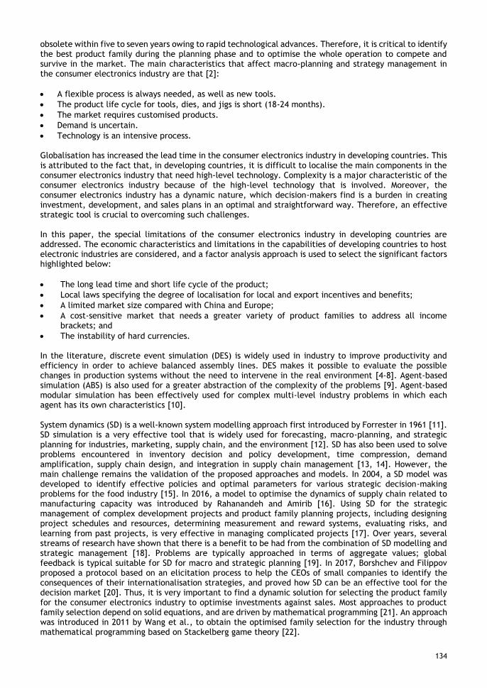
By setting the product design matrix, a design thinking approach is set up for the selection of key specification factors to define the product families’ characteristics for electronic devices. A survey is carried out with local marketing experts, local manufacturing experts, and customers to define these factors. Those that are selected are the factors that define the size of the device/screen, the technology of transmission, the software capabilities, the resolution of the screen, inputs/outputs, the main processor, sound output, and the main function specifications. These factors are reflected in the clustering. The life cycle can be divided in three main stages after the introduction phase [31]. The first stage is the growth period of new products. The second stage is the maturity period of the product in the market, during which the products are in the saturation phase. The third stage is the decline of the product in the market. The typical life cycle of a product is illustrated in Figure 2. In these studies, the families are categorised in three main classes that reflect these three periods. In the consumer electronics industry, the three different types of family are to be planned in the product portfolio. Through system dynamics simulation, we define the characteristics of each family and its response to the market, manufacture, supply chain, and new investments factors.

138

Figure 2: Product family life cycle

3 THE DEVELOPED SYSTEM DYNAMICS SIMULATION MODEL

This section is dedicated to explaining the developed simulation model, which is classified into three sub-models. Table 1 illustrates the model’s nomenclature.

Table 1: Model variables and description

Symbol Variable Description

t Time Time interval

𝑷𝑫𝒄𝒔𝒕 Planned_cost_development The planned cost per family owing to the estimation of development process

𝑺𝒂𝒄𝒕 Actual_for_sales_per_family The forecast sales for each family per week

𝑴𝑻𝑹𝒂𝒄𝒕 Actual_material_cost The actual material cost owing to actual market

𝑺𝑪𝑴𝒄𝒔𝒕 Supply_chain_and_manufacture_actual_cost The actual supply chain and manufacturing cost per product family

𝑺𝑪𝑺𝒓𝒕 Supply_chain_shipment_rate The rate for supply chain shipment

𝑺𝑪𝑯𝑫𝒂𝒄𝒕 actual_schedule The schedule of the time interval of development for a product family in weeks

𝐒𝐂𝐇𝐃𝐭𝐫 target_schedule The target of the time interval schedule to achieve the project’s development

𝐂𝐀𝐏𝐞𝐧𝐠 engineering_capacity The capacity of in-house engineers

𝐂𝐀𝐏𝐩𝐫𝐭 Partners_man_capacity The capacity of engineers of outsourcing partners

𝑺𝑪𝑯𝑫𝒄𝒔𝒕 Schedule_Engineering_Cost The cost in man-hours of developing engineers

𝑴𝑯𝑫𝒄𝒔𝒕 cost_of_development_of_man_hour The cost of development of product family as man-hours of engineering

𝑷𝑺𝑪𝒄𝒔𝒕 Planned_supply_chain_cost The planned cost of supply chain per family of products

𝑴𝑻𝑹𝒕𝒓𝒄𝒔𝒕 Target_Material_cost_per_family The target of material cost per product planning cost

𝑳𝑪𝒎𝒊𝒏𝒄𝒔𝒕 min_localisation_cost The minimum localisation ratio needed per law of localisation

𝑺𝒇𝒄𝒔𝒕 forecast_per_actual_family_product The forecast for actual sales

𝑴𝑺𝒂𝒄𝒕𝑭 Actual_Family_market_share The market share per family

𝑨𝑫𝒆𝒇𝒌𝒕 Advertising_effect The coefficient for advertising effect in the market

𝑵𝑻𝑪𝑯𝒊𝒎𝒑𝒌𝒕 New_technology_actual_impact The coefficient of impact of the market on new technology

𝑴𝑲𝑻𝒔𝒕 market_situation The coefficient of the market situation

𝑻𝑹𝒆𝒇𝒌𝒕 TR_market_effect The trend effect of the change of the raw material per time

𝑻𝑹𝒃𝒏𝒄𝒉 Price_targeted_Market This is the target price that is set by marketing to reach the target profit

𝑷𝑫𝒄𝒔𝒕 Planned_Cost_Design The planned cost of design

𝑺𝑪𝑯𝑫𝒕𝒓 Target_schedule_design The schedule is target for design

𝑴𝑭𝑮𝒄𝒔𝒕 Manufacture_cost The manufacturing cost per family

𝑺𝑪𝒄𝒐𝒔𝒕 Supply_chain_cost The supply chain cost per family

𝑴𝑭𝑮𝒄𝒂𝒑 Manufacture_capacity The production capacity

𝑸𝒄𝒔𝒕 Quality_cost The quality cost

139

Symbol Variable Description

𝑷𝑹𝒓𝒕 Production_rate The production rate

𝑺𝑪𝒓𝒕 Supply_Chain_Rate The rate for the supply chain to ship manufactured goods to market

𝑺𝑪𝑵𝑻𝒄𝒔𝒕𝒐𝒗 subcontracting_cost_over_time_per_family The overtime for subcontracting per family

𝑺𝑪𝑵𝑻𝒓𝒕 Subcontracting_rate The rate of shipment for subcontracting

𝑷𝑺𝑪𝒕𝒓𝒄𝒔𝒕 Planned_supply_chain_cost_target_material_cost_per_family

The planned supply chain cost of the selected family

𝑸𝒎𝒕𝒙 quality_matrix The matrix for the needed quality standards

𝑷𝑷𝑫𝒇𝒎𝒔𝒑 PPD_family_spec The planned specifications of the family

𝑩𝑲𝒄𝒔𝒕 Backorder_carrying_cost The cost of a backorder

𝑹𝑴𝑻𝑹𝒄𝒔𝒕 raw_material_carrying_cost_per_family The carrying cost for raw material

𝑷𝑹𝑶𝑫𝒐𝒗𝒓𝒕 Production_Rate_Overtime The production rate during overtime

𝑴𝑯𝒄𝒔𝒕 The man-hour cost The man-hour cost during regular working hours

𝑶𝑽𝑻𝒄𝒔𝒕 Overtime_cost The man-hour cost during overtime

𝑰𝑵𝑽𝒇𝒈 Finished_Products_Inventory The inventory of the finished goods

𝑶𝒃𝒌 Backlog_Orders The backlog orders

𝑻𝒔𝒉 Shipment_time The lead time for shipment to market

3.1 Model structure and relations between variables

The system dynamics modelling tool iThink® was used to simulate the dynamics and to conduct multiple scenarios to select the best plan. In order to simulate different scenarios for selecting the product families, a combination of demand, capacity options, and dynamic strategies were considered. In order to monitor and control the model variables more easily, the simulation model was divided into three sub-models. The first sub-model was developed to simulate market behaviour. The second sub-model was developed to describe the operation of the development and engineering of new product models. The third sub-model simulated the dynamics of supply and production for the consumer electronics industry, and its behaviour in response to the introduction of new technologies. Each main model was divided into many sub-models to ease the monitoring and control of the variables for different possible scenarios. The array function in iThink was used to describe the different families. In some equations, a 2D array is used to describe the link between the family and its specifications. Figure 3 describes the main interaction between the three models. In sub-model 1, the market activities of families are simulated. In sub-model 2, the development cost is calculated and used in sub-model 1 to calculate the total profit. In sub-model 3, we calculate the material, manufacturing, and supply costs, and supply a rate to calculate the total profit in sub-model 1. In sub-model 2, the actual sales from sub-model 1 are also used in the simulation

Figure 3: Model layout

The main relationships between families and new technologies describe the interaction between the different sub-models. In the model, equations are developed to describe the product family behaviours in the planning phase, in the supply chain, during manufacture, and in a real market situation. The equations are used to form the literature for product design, supply chain, and manufacturing as common equations, and are adapted by the coefficients that are proposed for this study. The coefficients are obtained through data correlations for each case study. The coefficients are for the technology effects in marketing, the supply chain, the manufacturing chain, and development. The equations below are calculated for each family.

Sub-model 1

Sub-model 2

Sub-model 3

𝑷𝑫𝒄𝒔𝒕

𝑺𝒂𝒄𝒕

𝑺𝑪𝑴𝒄𝒔𝒕 , 𝑴𝑻𝑹𝒂𝒄𝒕 & 𝑺𝑪𝒓𝒕

140

Equation (1) explains the product development cost, depending on the time needed to develop, the cost of the development engineers, the cost of localisation tools, and the planned supply chain and forecast material costs.

𝑷𝑫𝒄𝒔𝒕 = ∫ (𝑺𝑪𝑯𝑫𝒂𝒄𝒕 ∗ 𝑴𝑯𝑫𝒄𝒔𝒕) + 𝑳𝑪𝒎𝒊𝒏𝒄𝒔𝒕 + 𝑷𝑺𝑪𝒄𝒔𝒕 + 𝑴𝑻𝑹𝒕𝒓𝒄𝒔𝒕𝒕

𝟎dt (1)

Equation (2) explains the actual sales as a factor of forecast sales, which are affected by the advertisement coefficient, the market situation coefficients, and the impact of new technology that is introduced, which is zero for the products that are not introduced during that year.

𝑺𝒂𝒄𝒕 = ∫ ( 𝑺𝒇𝒄𝒔𝒕 ∗ 𝑴𝑺𝒂𝒄𝒕𝑭 ∗ 𝑨𝑫𝒆𝒇𝒌𝒕 ∗ 𝑵𝑻𝑪𝑯𝒊𝒎𝒑𝒌𝒕 ∗ 𝑴𝑲𝑻𝒔𝒕) 𝐝𝐭𝒕

𝟎 (2)

In equation (3), the material cost is calculated, depending on the forecast material cost, using the coefficient of the current trend of the material.

𝑴𝑻𝑹𝒂𝒄𝒕 = 𝑹𝑴𝑻𝑹𝒄𝒔𝒕 ∗ 𝑻𝑹𝒆𝒇𝒌𝒕 (3)

In equation (4), the rate of shipment to market is calculated.

𝑺𝑪𝒓𝒕 = ∫ (( 𝑀𝐼𝑁 (𝐼𝑁𝑉𝑓𝑔 ,𝑂𝑏𝑘)

𝑇𝑠ℎ) 𝑑𝑡

𝑡

0 (4)

3.1.1 The first sub-model

In Figure 4, the stock and flow diagram of sub-model 1 is described. This model is the output model of our simulation model, where market activities are simulated, and total sales and total profit are calculated. The sub-model is divided into 4 sectors. In forecast sector, the forecast for new family depending on time series forecast Box-Jenkins recommendations as explained in section 2 is simulated. The historical data is

entered in graphical representations. The forecasting is calculated according to ∅𝝆(𝑩)𝝑𝑷(𝑩)(𝟏 − 𝑩)𝒅(𝟏 −

𝑩𝒔)𝑫 𝑿𝒕 = 𝜽𝒒 (𝑩)𝝋𝑸 (𝑩𝒔)𝒂𝒕 equation where is s is calculated as seasons of selected product. d, D, 𝝆, q, P,

and Q as our data coloration and to simplify the models is used to be 1. Decision will be owing to planned cost owing to spec, engineering, capacity and target because of the bench market. As a result of the decision sector, quantity will be reducing by percentage because of achieving the target owing to marketing coefficient. Equation (5) relates the variables for each family: 𝑖𝑓 𝑇𝑅𝑏𝑛𝑐ℎ < 𝑃𝐷𝑐𝑠𝑡 𝑡ℎ𝑒𝑛 1 𝑒𝑙𝑠𝑒 = 𝑓𝑐 (5) where fc is the coefficient of portion of the marketing team reduction of the coefficient’s target. In the sector of the actual market, sales will be simulated, and the effect of the market situation, the actual impact of new technology, the advertising impact, and the actual costs of manufacturing and the supply chain will be transferred from the manufacturing and supply chain model. Total profit, market share, and total revenue will be monitored. Each family can be monitored separately for sales and profit. Total profit is calculated as below in equation (6): Profit = market price – raw material cost – total supply chain cost – inventory cost (6) In this model, the price of the developed module is imported from the development model. The cost of manufacturing and the supply chain is developed from the manufacturing and supply chain model.

3.1.2 The second sub-model

The stock and flow diagram of the development and engineering model is described in Figure 5. As the engineering capacity sub-model, the needed man capacity is calculated. In the specification change effect sector, the new technology selection process is simulated. A new specification coefficient is calculated. In the quality sectors, the target quality of the needed specification is simulated.

The schedule calculation process is simulated according to target quality. For the cost of parts, the planned cost of development is calculated as man-hours (7):

𝑆𝐶𝐻𝐷𝑐𝑠𝑡 = 𝑀𝐻𝐷𝑐𝑠𝑡 ∗𝑆𝐶𝐻𝐷𝑡𝑟

0.01∗(𝐶𝐴𝑃𝑝𝑟𝑡 + 𝐶𝐴𝑃𝑒𝑛𝑔) (7)

141

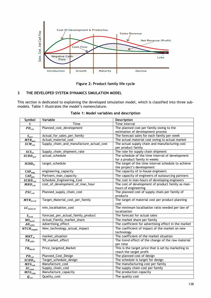
Figure 4: Stock and flow diagram with causal loops for sub-model 2

In the quality sectors, the quality deployment needed for the selected specifications is determined and simulated. The specifications and its family depend on the current profile and the forecast of the new specification. Quality deployment for design is considered as below, in equation (8):

𝑰𝑭 𝑸𝒎𝒕𝒙 > 𝟎 𝒕𝒉𝒆𝒏 = 𝑷𝑷𝑫𝒇𝒎𝒔𝒑 𝒆𝒍𝒔𝒆 = 𝟎 (8)

142

Figure 5: Stock and flow diagram with causal loops for sub-model 2

3.1.3 The third sub-model

In this study, the model of Abouzar et al. [32] is adapted to be suitable for the consumer electronics industry, and to accommodate different features of our case and so be integrated into the other sub-models. In Figure 6, the stock and flow diagram of the supply chain and manufacturing model is explained. For the cost part, the planned cost is calculated per family, based on the development cost of the engineering, the material cost according to specifications, the manufacturing cost because of tools and localisation, and the standard supply chain cost. In Figure 6, the third sub-model is divided into five sectors. The raw material and components sectors cover the aspects of changing specifications and technology for the material inventory plan. The material cost sector has the role of forecasting the raw material. The raw material for consumer electronics has the special characteristics of price changes as a result of capacity and demand, as well as technology changes. Historical data is used to forecast the prices of raw material, based on time series forecasting. Thus many aspects of the dynamics in change of capacity, new material owing to technology, prices of raw materials, and variable demand are used in our model to forecast the total cost of the supply chain and manufacturing. In the overtime sector, the overtime cost is simulated. In the regular time sector, the cost of manufacturing according to capacity on the basis of the needed technology is simulated. The inventory level is simulated in the productivity per inventory sector. In the order rate sector, the supply chain rate is simulated. As all five sectors interact, equations (9) and (10) below describe the cost calculation for the supply chain and manufacturing cost, calculated from the inventory cost, production rate, capacity, and overtime calculations:

𝑺𝑪𝒄𝒔𝒕 = 𝑩𝑲𝒄𝒔𝒕 ∗ 𝑹𝑴𝑻𝑹𝒇𝒄𝒔𝒕 (9)

𝑴𝑭𝑮𝒄𝒔𝒕 = ∫ ( 𝑷𝑹𝒓𝒕 ∗ 𝑴𝑭𝑮𝒄𝒔𝒕) + (𝑷𝑹𝑶𝑫𝒐𝒗𝒓𝒕 ∗ 𝑶𝑽𝑻𝒄𝒔𝒕) + (𝑺𝑪𝑵𝑻𝒄𝒔𝒕𝒐𝒗 ∗ 𝑺𝑪𝑵𝑻𝒓𝒕)𝒕

𝟎 dt (10)

These two variables are the main variables along with design cost and marketing cost, which affect the total cost of the model and so also the total profit of the model.

3.2 Simulation conditions

The software package iThink was used to perform the simulations. It is iconographic software that uses basic building blocks such as stocks, flows, and converters, as shown in Figures 4, 5, and 6. The simulations made it possible to run all three sub-models as one model for the selected number of weeks, and the software enabled us to use a two-dimensional array as well as a time graph to input the needed data.

143

Figure 6: Stock and flow diagram with causal loops for sub-model 3

4 CASE STUDY

A television (TV) manufacturing company where the technology changes frequently was chosen as the application case study. As the study has indicated, sets are widely manufactured in developing countries, and local production is protected by local laws; thus it is believed to be a good example to validate the developed model. TV technology has changed rapidly in the past few years, from CRT to liquid crystal display (LCD) TV to light-emitting diode (LED) LCD TV to Organic LED (OLED) and micro-LED technology [33].

Backlog of Orders

market order rate

Fulf illed Orders

av erage period f or production

in ov ertime

Backorder carry ing cost

desired production

lev el ov er time

planed setup timeno of f amilies

weeks raw material rate

max capacity

ov ertime

raw material f or ov er time

Finished Products Inv entory

Shipment Rate

Subcontracting rate

Time to Subcontract

Total Production Cost

raw material cost

trend delay

~

av erage production in ov ertime

Shipment Time

max capacity in regular

time

buf f er day s f or f amiles

new technology cof f icient

no of f amilies f or buf f er

Production Rate

weeks needed f or

ov er time

Family productiv ity

av erage production rate

in regular time

learning cof f icent f or new

technology regular time

item f or new

technology

Av erage Period

f or Order Rate

manf acture

cost

setup time in ov er time

Av erage Order Rate

raw material carry ing

cost per f amilybackorder cost

no of f amilies f or

orders rate

production rate in ov ertime

Workf orce Lev el

in Regular Time

Hiring Rate in

Regular Time

Resign

manf actue cost regular time

per f amily

manf actue cost ov er time

per f amily 2

subcotracting cost ov er time

per f amily 3

Desired Workf orce

Lev el in Regular Time

cost

weeks av aliable

raw material trend price rate

~

Raw Materials Inv entory

Raw Materials

Arriv al Rate

Raw Materials

Departure Rate

desired Raw Materials

desired inv entory

Raw Materials

Order Rate time to order

Marketing and forecast.sales from

market per family

OC market ef f ect

Av erage Period f or Production

Rate in Regular Time

Total Carry ing and

Backordering Costs

ov ertime situation

order rate

regular time work

Productiv ity per inv entory

Raw material and key components inv entory

Total production cost Material cost

delay

delay

delay

144

The case study is for a major industrial and market stakeholder company in Egypt that is one of the big three players in the local market. The company produces and sells about one million TV sets of different sizes and technologies each year, in an average of 80 to 100 product variations. We simulated the profit made and the pattern of sales. The product family is produced for 108 weeks of the year, on average. The different families represent new technologies, growing technologies, saturated technologies, and decaying technologies. Egypt’s TV market has been studied well, and the historical data for the whole market has been collected by a market research company. The case study company provided their data for sales, manufacturing, and supply chain for the period from 2017 to 2019.

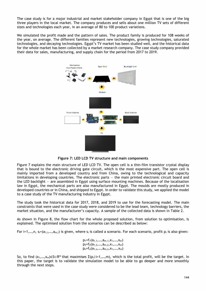
Figure 7: LED LCD TV structure and main components

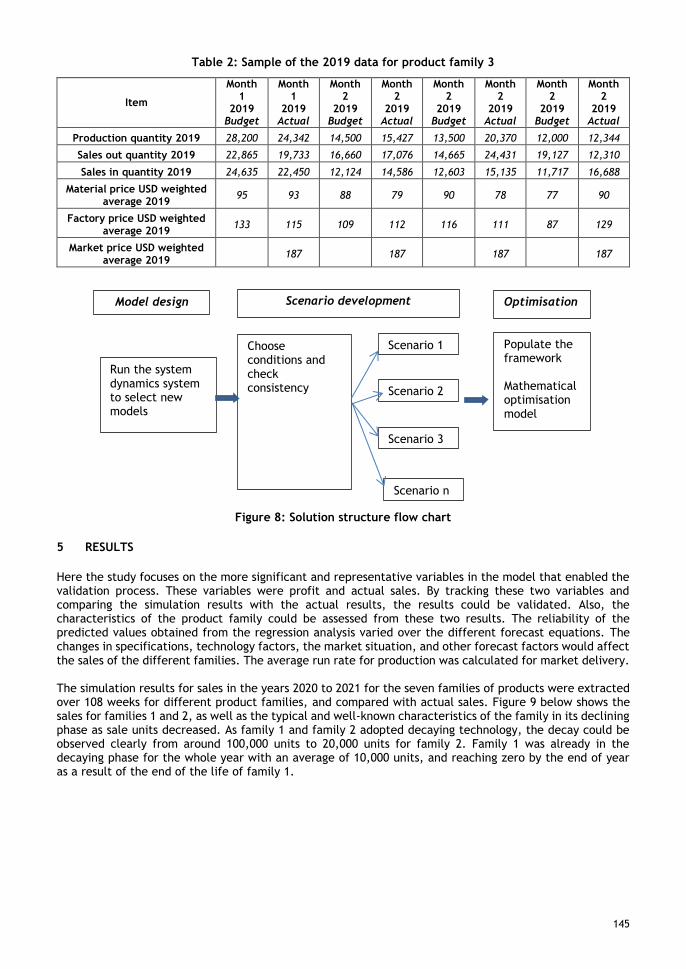
Figure 7 explains the main structure of LED LCD TV. The open cell is a thin-film transistor crystal display that is bound to the electronic driving gate circuit, which is the most expensive part. The open cell is mainly imported from a developed country and from China, owing to the technological and capacity limitations in developing countries. The electronic parts — the main printed electronic circuit board and the LED backlight — are assembled in Egypt using surface mounting machines. Because of the localisation law in Egypt, the mechanical parts are also manufactured in Egypt. The moulds are mostly produced in developed countries or in China, and shipped to Egypt. In order to validate this study, we applied the model to a case study of the TV manufacturing industry in Egypt. The study took the historical data for 2017, 2018, and 2019 to use for the forecasting model. The main constraints that were used in the case study were considered to be the lead team, technology barriers, the market situation, and the manufacturer’s capacity. A sample of the collected data is shown in Table 2. As shown in Figure 8, the flow chart for the whole proposed solution, from solution to optimisation, is explained. The optimised solution from the scenarios can be described as below: For i=1,…,n, si=(a1,i,…,am,i) is given, where si is called a scenario. For each scenario, profit pi is also given:

p1=f1(a1,1,…,am,1,x1,…,xm) p2=f2(a1,2,…,am,2,x1,…,xm) pn=fn(a1,n,…,am,n,x1,…,xm)

So, to find (x1,…,xm)∈S⊂Rm that maximises Σ(pi|i=1,…,m), which is the total profit, will be the target. In this paper, the target is to validate the simulation model to be able to go deeper and more smoothly through the next steps.

145

Table 2: Sample of the 2019 data for product family 3

Item

Month 1

2019 Budget

Month 1

2019 Actual

Month 2

2019 Budget

Month 2

2019 Actual

Month 2

2019 Budget

Month 2

2019 Actual

Month 2

2019 Budget

Month 2

2019 Actual

Production quantity 2019 28,200 24,342 14,500 15,427 13,500 20,370 12,000 12,344

Sales out quantity 2019 22,865 19,733 16,660 17,076 14,665 24,431 19,127 12,310

Sales in quantity 2019 24,635 22,450 12,124 14,586 12,603 15,135 11,717 16,688

Material price USD weighted average 2019

95 93 88 79 90 78 77 90

Factory price USD weighted average 2019

133 115 109 112 116 111 87 129

Market price USD weighted average 2019

187 187 187 187

Figure 8: Solution structure flow chart

5 RESULTS

Here the study focuses on the more significant and representative variables in the model that enabled the validation process. These variables were profit and actual sales. By tracking these two variables and comparing the simulation results with the actual results, the results could be validated. Also, the characteristics of the product family could be assessed from these two results. The reliability of the predicted values obtained from the regression analysis varied over the different forecast equations. The changes in specifications, technology factors, the market situation, and other forecast factors would affect the sales of the different families. The average run rate for production was calculated for market delivery. The simulation results for sales in the years 2020 to 2021 for the seven families of products were extracted over 108 weeks for different product families, and compared with actual sales. Figure 9 below shows the sales for families 1 and 2, as well as the typical and well-known characteristics of the family in its declining phase as sale units decreased. As family 1 and family 2 adopted decaying technology, the decay could be observed clearly from around 100,000 units to 20,000 units for family 2. Family 1 was already in the decaying phase for the whole year with an average of 10,000 units, and reaching zero by the end of year as a result of the end of the life of family 1.

Run the system dynamics system to select new models

Model design

Scenario development

Choose conditions and check consistency

Optimisation

Scenario 1

Scenario 2

Scenario 3

Scenario n

Populate the framework Mathematical optimisation model

146

Figure 9: Sales for family 1 and family 2

The sales of families 3, 4, and 5 are shown in Figure 10. These families were those that sold the most, and were the company’s ‘cash cows’. They were in the maturation phase. The averages sales for families 3 and 4 in the second year were around 200,000 units, while family 5 sold on average, 100,000 units in the second year. These families dominated the market share. The technology of these families was stable and already experienced good demand. The simulation results reflected the situation of these families in the actual market. The sales of families 6 and 7 are shown in Figure 11. These families had very limited sales, even though they contained the flagship products — for this case study, the Android TV and OLED models. In the Egyptian market, these products were sold in limited numbers; so these results could reflect the real market. By studying the sales of different families, the location of each family in the product life cycle can be determined. Using this analysis, the result of the simulation for each family can easily be compared with the real market.

Figure 10: Sales for family 3, family 4, and family 5

0.00

20 000.00

40 000.00

60 000.00

80 000.00

100 000.00

120 000.00

140 000.00

1 6

11

16

21

26

31

36

41

46

51

56

61

66

71

76

81

86

91

96

10

1

10

6

Sale

s in

un

its

Time in weeks

Family1 Family 2

0.00

50 000.00

100 000.00

150 000.00

200 000.00

250 000.00

1 6

11

16

21

26

31

36

41

46

51

56

61

66

71

76

81

86

91

96

10

1

10

6

Sale

s in

un

its

Time in weeks

Family 3 Family 4 Family 5

147

Figure 11: Sales for family 6 and family 7

Figure 12: Profit results for family 1 and family 2

Figure 13: Profit results for family 3, family 4, and family 5

0

500

1000

1500

2000

2500

3000

3500

4000

1 6

11

16

21

26

31

36

41

46

51

56

61

66

71

76

81

86

91

96

10

1

10

6

Sale

s in

un

its

Time in weeks

Family 6 Family 7

-2 000 000.00

0.00

2 000 000.00

4 000 000.00

6 000 000.00

8 000 000.00

10 000 000.00

12 000 000.00

1 7

13

19

25

31

37

43

49

55

61

67

73

79

85

91

97

10

3

10

9

Pro

fit

in E

GP

Time (weeks)

Family 1 Family 2

-20 000 000.00

-10 000 000.00

0.00

10 000 000.00

20 000 000.00

30 000 000.00

40 000 000.00

1 7

13

19

25

31

37

43

49

55

61

67

73

79

85

91

97

10

3

10

9

Pro

fit

in E

GP

Time (weeks)

Family 3 Family 4 Family 5

148

Figure 14: Profit results for family 6 and family 7

The results show that the model incorporated all of the factors driving sales, design, income per supply chain, and manufacturing activity, and reflected them for the output of sales and profit. This study could therefore conclude that our model could be selected as the most appropriate one to reflect system dynamics in the consumer electronics industries in developing countries.

6 CONCLUSION AND FUTURE WORK

In this paper, a new methodology was developed to decide the production plan for new families among the current options of new technology in consumer electronics industries in developing countries. The methodology adopted the key factors in marketing, supply chain, manufacturing, and design to be used for the simulation. The methodology used for forecasting depended on the historical production data of different products, with time series forecasting using Box-Jenkins. A system dynamics models was designed in our study to simulate the system dynamics environment of consumer electronics businesses in developing countries, and it integrated well with family clustering and time series forecasting. Three sub-models were developed to simulate three different stages. The first was for the market dynamics; the second was for the design and development dynamics; and the third was for the supply chain and manufacturing dynamics. The model was built using iThink as a system dynamics tool. As a next step, the study will examine the different scenarios, and the key variables that determines the product family selection. This shows how profit is sensitive to technological changes and to the behaviour in the market resulting from the new technology. Different scenarios will be generated to select the best planning strategy from the available scenarios. The final step will be to develop the optimisation system, based on different scenarios for different key variables. The study will include the use of linear programming to obtain an optimised solution.

REFERENCES

[1] Şeker, S. & Özgürler, M. 2012. Analysis of the Turkish consumer electronics firm using SWOT-AHP method. Procedia — Social and Behavioral Sciences, 58(12), pp. 1544-1554.

[2] Chen, J.H. and Jan, T.S. 2005. A system dynamics model of the semiconductor industry development in Taiwan. Journal of the Operational Research Society, 56(10), pp. 1141-1150.

[3] Lim, L., Alpan, G. & Penz, B. 2016. A simulation-optimization approach for sales and operations planning in build to-order industries with distant sourcing: Focus on the automotive industry. Journal of Computers & Industrial Engineering, 112, pp. 469-482.

[4] Banks, J., 1998. Handbook of simulation: principles, methodology, advances, applications, and practice. John Wiley & Sons.

[5] Pidd, M. 1998. Computer simulation in management science, 4th ed. New York: John Wiley & Sons. [6] Ferro, R., Cordeiro, G.A. & Ordoñez, R.E.C. 2018. Dynamic modeling of discrete event simulation. ICCMS 2018:

The 10th International Conference on Computer Modeling and Simulation, January 8-10, pp. 248–252.

-1 000 000.00

0.00

1 000 000.00

2 000 000.00

3 000 000.00

4 000 000.00

5 000 000.00

1 7

13

19

25

31

37

43

49

55

61

67

73

79

85

91

97

10

3

10

9

Pro

fit

in E

GP

Time (weeks)

Family 6 Family 7

149

[7] Salama, S. and Eltawil, A.B. 2018. A decision support system architecture based on simulation optimization for cyber-physical systems. Procedia Manufacturing, 26, pp.1147-1158.

[8] Abdelkhak, M., Salama, S. & Eltawil, A.B. 2018. Improving efficiency of TV PCB assembly line using a discrete event simulation approach — A case study. 10th International Conference on Computer Modeling and Simulation, ICCMS 2018.

[9] Negmeldin, M.A. & Eltawil, A. 2015. Agent based module in factory planning and process control. 50th IEEE International Conference on Industrial Engineering and Engineering Management, IEEM2015.

[10] Barbosa, J. and Leitão, P. 2011, July. Simulation of multi-agent manufacturing systems using agent-based modelling platforms. In 2011 9th IEEE International Conference on Industrial Informatics (pp. 477-482). IEEE.

[11] Saraji, M.K. and Sharifabadi, A.M. 2017. Application of system dynamics in forecasting: a systematic review. International Journal of Management, Accounting and Economics, 4(12), pp.1192-1205.

[12] Borshchev, A. & Filippov, A. 2004. From system dynamics and discrete event to practical agent based modeling: Reasons, techniques, tools. The 22nd International Conference of the System Dynamics Society, Oxford, England.

[13] Dey, D. & Sinha, D. 2019. A literature review based on the uses of system dynamics model in the perspective of supply chain Journal of. the Gujarat Research Society, 21 (14).

[14] Rebs, T., Brandenburg, M. & Seuring, S. 2019. System dynamics modeling for sustainable supplychain management: A literature review and systems thinking approach. Journal of Cleaner Production, 208, pp. 1265-1280.

[15] Georgiadis, P., Vlachos, D. & Iakovou, E. 2005. A system dynamics modeling framework for the strategic supplychain management of food chains. Journal of Food Engineering, 70, pp. 351-364.

[16] Rahanandeh, R. & Amirib, M. 2016. A system dynamics modeling approach for a multi-level, multi-product, multi-region supplychain under demand uncertainty. Journal of Expert Systems with Applications, 51, pp. 231–244.

[17] Lyneis, J.M., Cooper, K.G. & Els, S.A. 2001. Strategic management of complex projects: A case study using system dynamics. Journal of System Dynamics Review, 17(3), pp. 237–260.

[18] Cosenz, F. & Noto, G. 2016. Applying system dynamics modelling to strategic management: A literature review. Journal of Systems Research and Behavioral Science, 33, pp. 703-741.

[19] Heshmat, M. and Eltawil, A. 2016, May. A system dynamics model for chemotherapy. In Proceedings of the 10th international conference on informatics and systems (pp. 7-13).

[20] Torres, J.P., Kunc, M. & O’Brien, F. 2017. Supporting strategy using system dynamics. European Journal of Operational Research, 260(3), pp. 1081-1094.

[21] Simpson, T.W., Siddique, Z. and Jiao, R.J. 2006. Product platform and product family design: methods and applications. Springer Science & Business Media.

[22] Wang, D., Du, G., Jiao, R.J., Wu, R., Yu, J. & Yang, D. 2016. A Stackelberg game theoretic model for optimizing product family architecting with supply chain consideration. Int. J. Production Economics, 172, pp. 1-18.

[23] Chatfield, C. 2000. Time-series forecasting. CRC press. [24] Wada, Y., Hamada, K., Hirata, N., Seki, K. & Yamada, S. 2018. A system dynamics model for shipbuilding demand

forecasting. Journal of Marine Science and Technology, 23, pp. 236–252. [25] Ivanov, D. 2017. Simulation-based single vs. dual sourcing analysis in the supply chain with consideration of

capacity disruptions, big data and demand patterns. International Journal of Integrated Supply Management, 11(1), pp.24-43

[26] Oh, Y.-Y., Yun, S.-T., Yu, S. & Hamm, S.-Y. 2017. The combined use of dynamic factor analysis and wavelet analysis to evaluate latent factors controlling complex groundwater level fluctuations in a riverside alluvial aquifer. Journal of Hydrology, 555, pp. 938-955.

[27] García-Jurado, I., González-Manteiga, W., Prada-Sánchez, J.M., Febrero-Bande, M. & Cao, R. 1995. Predicting using Box-Jenkins, nonparametric, and bootstrap techniques. Technometrics, 37, pp. 303-310.

[28] Dalrymple, D.J. 1978. Using Box-Jenkins techniques in sales forecasting. Journal of Business Research, 6(2), pp.133-145.

[29] Heshmat, M., Nakata, K. & Eltawil, A. 2018. Solving the patient appointment scheduling problem in outpatient chemotherapy clinics using clustering and mathematical programming. Journal of Computers & Industrial Engineering, 124, pp. 347–358.

[30] Comaniciu, D. & Meer, P. 2002. Mean shift: A robust approach toward feature space analysis. IEEE Transactions on Pattern Analysis and Machine Intelligence, 24(5), 603–619.

[31] Anderson, C.A. & Zeithaml, C.P. 1984. Stage of the product life cycle, business strategy, and business performance. Academy of Management Journal, 27(I), pp. 5-24.

[32] Jamalnia, A. and Feili, A. 2013. A simulation testing and analysis of aggregate production planning strategies. Production Planning & Control, 24(6), pp.423-448.

[33] Huang, Y., Hsiang, E.L., Deng, M.Y. and Wu, S.T. 2020. Mini-LED, Micro-LED and OLED displays: Present status and future perspectives. Light: Science & Applications, 9(1), pp.1-16.