A survey on algorithmic aspects of modular decomposition

A Survey on Algorithmic Aspects of

Modular Decomposition∗

Michel Habib† Christophe Paul‡

December 10, 2009

Abstract

The modular decomposition is a technique that applies but is not restricted to graphs.The notion of module naturally appears in the proofs of many graph theoretical theorems.Computing the modular decomposition tree is an important preprocessing step to solve a largenumber of combinatorial optimization problems. Since the first polynomial time algorithm in theearly 70’s, the algorithmic of the modular decomposition has known an important development.This paper survey the ideas and techniques that arose from this line of research.

1 Introduction

Modular decomposition is a technique at the crossroads of several domains of combinatorics whichapplies to many discrete structures such as graphs, 2-structures, hypergraphs, set systems and ma-troids among others. As a graph decomposition technique it has been introduced by Gallai [Gal67]to study the structure of comparability graphs (those graphs whose edge set can be transitivelyoriented). Roughly speaking a module in graph is a subset M of vertices which share the sameneighbourhood outside M . Galai showed that the family of modules of an undirected graph can berepresented by a tree, the modular decomposition tree. The notion of module appeared in the lit-terature as closed sets [Gal67], clan [EGMS94], automonous sets [Moh85b], clumps [Bla78]. . . whilethe modular decomposition is also called substitution decomposition [Moh85a] or X-join decompo-sition [HM79]. See [MR84] for an early survey on this topic.

There is a large variety of combinatorial applications of modular decomposition. Modules canhelp proving structural results on graphs as Galai did for comparability graphs. More generallymodular decomposition appears in (but is not limited to) the context of perfect graph theory. IndeedLovasz’s proof of the perfect graph theorem [Lov72] involves cliques modules. Notice also that anumber of perfect graph classes can be characterized by properties of their modular decompositiontree: cographs, P4-sparse graphs, permutation graphs, interval graphs. . . Refer to the books ofGolumbic [Gol80], Brandstadt et al. [BLS99] for graph classes. We should also mention that themodular decomposition tree is useful to solve optimization problems on graphs or other discretestructures (see [Moh85b]). An example of such use is given in the last section.∗Work supported by the French research grant ANR-06-BLAN-0148-01 “Graph Decompositions and Algorithms -

graal”.†LIAFA, Universite Paris 7 Diderot, France‡CNRS - LIRMM, Universite de Montpellier 2, France

1

arX

iv:0

912.

1457

v2 [

cs.D

M]

10

Dec

200

9

In the late 70’s, the modular decomposition has been independently generalized to partitive setfamilies [CHM81] and to a combinatorial decomposition theory [CE80] which applies to graphs,matroids and hypergraphs. More recently, the theory of partitive families and its variants hadbeen the foundation of decomposition schemes for various discrete structures among which 2-structures [EHR99] and permutations [UY00, BCdMR08]. Beside, based on efficiently representableset families, different graph decompositions had been proposed. The split decomposition of [CE80]relies on a bipartitive family on the vertex set. Refer to [BX08] for a survey on the recent develop-ments of these techniques.

A good feature of most of these decomposition schemes is that they can be computed in poly-nomial time. Indeed, since the early 70’s, there have been a number algorithms for computing themodular decomposition of a graph (or for some variants of this problem). The first polynomial algo-rithm is due to Cowan, James and Stanton [CJS72] and runs in O(n4). Successive improvements aredue to Habib and Maurer [HM79] who proposed a cubic time algorithm, and to Muller and Spinradwho designed a quadratic time algorithm. The first two linear time algorithms appeared indepen-dently in 1994 [CH94, MS94]. Since then a series of simplified algorithms has been published, somerunning in linear time [MS99, TCHP08], others in almost linear time [DGM01, MS00, HPV99]. Thelist is not exhaustive. This line of research yields a series of new interesting algorithmic techniques,which we believe, could be useful in other applications or topics of computer science. The aim ofthis paper is to survey the algorithmic theory of modular decomposition.

The paper is organized as follows. The partitive family theory and its application to modulardecomposition of graphs is presented in Section 2. As an algorithmic appetizer, Section 3 addressesthe special case of totally decomposable graphs, namely the cographs, for which a linear timealgorithm is known since 1985 [CPS85]. Partition refinement is an algorithmic technique thatreveals to be really powerful for the modular decomposition problem, but also for other graphsapplications (see e.g. [PT87, HPV99]). Section 4 is devoted to partition refinement. Section 5describes the principle of a series of modular decomposition algorithms developped in the mid90’s. Section 6 explains how the modular decomposition can be efficiently computed via the recentconcept of factoring permutation [CHdM02]. Let us mention that we do not discuss the recentlinear time algorithm of Tedder et al. [TCHP08], even though we believe that this last algorithmprovides a positive answer to the problem of finding a simple linear time modular decompositionalgorithm. Actually the key to Tedder et al.’s algorithm is to merge the ideas developed in Sections5 and 6. The purpose of this paper is not to enter into the details of all the algorithm techniques butrather to present their main lines. Finally the last section presents three recent applications of themodular decomposition in three different domains of computer science, namely pattern matching,computational biology and parameterized complexity.

2 Partitive families

The modular decomposition theory has to be understood as a special case of the theory of partitivefamily whose study dates back to the early 80’s [CE80, CHM81]. We briefly present the mainsconcepts and theorems of the partitive family theory. We then introduce the modular decompositionof graphs and discuss its elementary algorithmic aspects. This section ends with a discussion on twoimportant class of graphs: indecomposable graphs (the prime graphs) and totally decomposablegraphs (known as the cographs)

2

2.1 Decomposition theorem of partitive families

The symmetric difference between two sets A and B is denoted by A M B = (A \ B) ∪ (B \ A).Two subsets A and B of a set S overlap if A ∩B 6= ∅, A \B 6= ∅ and B \A 6= ∅, we write A ⊥ B.

Definition 1 A family S ⊆ 2S of subsets of S is partitive if:1. S ∈ S, ∅ /∈ S and for all x ∈ S, {x} ∈ S;

2. For any pair of subsets A,B ∈ S such that A ⊥ B:

(a) A ∩B ∈ S;

(b) A \B ∈ S and B \A ∈ S;

(c) A ∪B ∈ S;

(d) A M B ∈ S.

A family is weakly partitive whenever condition (2.d) is not satisfied. Unless explicitly men-tioned, we will only consider partitive families.

Definition 2 An element F ∈ S is strong if it does not overlap any other element of S. The setof strong elements of S is denoted SF .

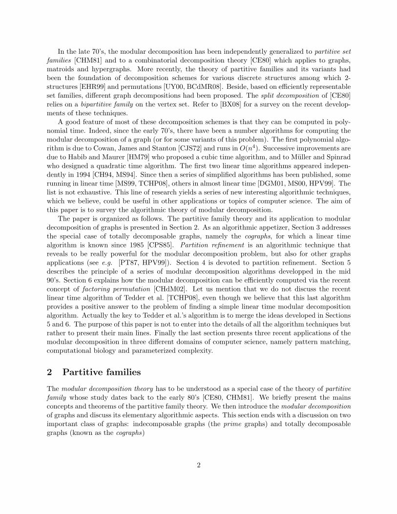
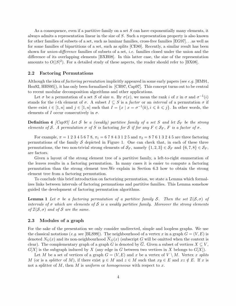
Obviously any trivial subset of S, namely S or {x} (for x ∈ S), is a strong element. Let usremark that SF is nested, i.e. the transitive reduction of the inclusion order of SF is a tree TS ,which we call the strong element tree (see Figure 1). It follows that |SF | = O(|S|).

Degenerate

2

3 8

7

61

5

4

Prime

Degenerate

1 2 3 4 5 6 7 8

Figure 1: The inclusion tree of the strong elements of the familyS = {{1, 2, 3, 4, 5, 6, 7, 8}, {1, 2, 3}, {6, 7, 8}, {1, 2}, {2, 3}, {1, 3}, {6, 7}, {7, 8}, {6, 8},{1}, {2}, {3}, {4}, {5}, {6}, {7}, {8}}

Definition 3 Let f q1 , . . . , f

qk be the chidren of a node q of TS , the strong element tree of S. The

node q is degenerate if for all non-empty subset J ⊂ [1, k], ∪j∈Jfqj ∈ S. A node is prime if for

every non-empty subset J ⊂ [1, k], ∪j∈Jfqj /∈ S.

It is not difficult to see that any strong element is either prime or degenerate. Moreover thefollowing theorem tells us that the tree TS is a representation of the family S and the subfamily ofstrong elements SF of S defines a ”basis” of S.

Theorem 1 [CHM81] Let S be a partitive family on S. The subset A ⊆ S belongs to S if and onlyif A is strong or there exists a degenerate strong element A′ (or a node of TS) such that A is theunion of a strict subset of the children of A′ in TS .

3

As a consequence, even if a partitive family on a set S can have exponentially many elements, italways admits a representation linear in the size of S. Such a representation property is also knownfor other families of subsets of a set, such as laminar families, cross-free families [EG97]. . . as well asfor some families of bipartitions of a set, such as splits [CE80]. Recently, a similar result has beenshown for union-difference families of subsets of a set, i.e. families closed under the union and thedifference of its overlapping elements [BXH08]. In this latter case, the size of the representationamounts to O(|S|2). For a detailed study of these aspects, the reader should refer to [BX08].

2.2 Factoring Permutations

Although the idea of factoring permutation implicitly appeared in some early papers (see e.g. [HM91,Hsu92, HHS95]), it has only been formalized in [CH97, Cap97]. This concept turns out to be centralto recent modular decomposition algorithms and other applications.

Let σ be a permutation of a set S of size n. By σ(x), we mean the rank i of x in σ and σ−1(i)stands for the i-th element of σ. A subset I ⊆ S is a factor or an interval of a permutation σ ifthere exist i ∈ [1, n] and j ∈ [1, n] such that I = {x | x = σ−1(k), i 6 k 6 j}. In other words, theelements of I occur consecutively in σ.

Definition 4 [Cap97] Let S be a (weakly) partitive family of a set S and let SF be the strongelements of S. A permutation σ of S is factoring for S if for any F ∈ SF , F is a factor of σ.

For example, π = 1 2 3 4 5 6 7 8, π1 = 6 7 8 4 3 1 2 5 and π2 = 8 7 6 1 3 2 4 5 are three factoringpermutations of the family S depicted in Figure 1. One can check that, in each of these threepermutations, the two non-trivial strong elements of SF , namely {1, 2, 3} ∈ SF and {6, 7, 8} ∈ SF ,are factors.

Given a layout of the strong element tree of a partitive family, a left-to-right enumeration ofthe leaves results in a factoring permutation. In many cases it is easier to compute a factoringpermutation than the strong element tree.We explain in Section 6.3 how to obtain the strongelement tree from a factoring permutation.

To conclude this brief introduction on factorizing permutation, we state a Lemma which formal-izes links between intervals of factoring permuations and partitive families. This Lemma somehowguided the development of factoring permutation algorithms.

Lemma 1 Let σ be a factoring permutation of a partitive family S. Then the set I(S, σ) ofintervals of σ which are elements of S is a weakly partitive family. Moreover the strong elementsof I(S, σ) and of S are the same.

2.3 Modules of a graph

For the sake of the presentation we only consider undirected, simple and loopless graphs. We usethe classical notations (e.g. see [BLS99]). The neighbourhood of a vertex x in a graph G = (V,E) isdenoted NG(x) and its non-neighbourhood NG(x) (subscript G will be omitted when the context isclear). The complementary graph of a graph G is denoted by G. Given a subset of vertices X ⊆ V ,G[X] is the subgraph induced by X (any edge in G between two vertices in X belongs to G[X]).

Let M be a set of vertices of a graph G = (V,E) and x be a vertex of V \M . Vertex x splitsM (or is a splitter of M), if there exist y ∈ M and z ∈ M such that xy ∈ E and xz /∈ E. If x isnot a splitter of M , then M is uniform or homogeneous with respect to x.

4

Definition 5 Let G = (V,E) be a graph. A set M ⊆ V of vertices is a module if M is homogeneouswith respect to any x /∈M (i.e. M ⊆ N(x) or M ∩N(x) = ∅).

Observation 1 Let S be a subset of vertices of a graph G = (V,E). If S has a splitter x, then anymodule of G containing S also contains x.

Aside the singletons and the whole vertex sets, any union of connected components (or ofco-connected components) of a graph are simple examples of modules. Let us also note thata graph may have exponentially many modules. Indeed any subset of a complete graph is aclique. Nevertheless, as we shall see with the following lemma, the family of modules has strongcombinatorial properties.

Lemma 2 [CHM81] The family M of modules of a graph is partitive.

The notions of trivial and strong module and degenerate are defined according to the terminol-ogy of Section 2.1. By Lemma 2, if M and M ′ are overlapping modules, then M \M ′, M ′ \M ,M ∩M ′, M ∪M ′ and M MM ′ are modules of G.

Let M and M ′ be disjoint sets. We say that M and M ′ are adjacent if any vertex of M isadjacent to all the vertices of M ′ and non-adjacent if the vertices of M are non-adjacent to thevertices of M ′.

Observation 2 Two disjoint modules are either adjacent or non-adjacent.

A module M is maximal with respect to a set S of vertices, if M ⊂ S and there is no moduleM ′ such that M ⊂M ′ ⊂ S. If the set S is not specified, we shall assume S = V .

Definition 6 Let P = {M1, . . . ,Mk} be a partition of the vertex set of a graph G = (V,E). If forall i, 1 6 i 6 k, Mi is a module of G, then P is a modular partition (or congruence partition) ofG.

A non-trivial modular partition P = {M1, . . . ,Mk} which only contains maximal strong modulesis a maximal modular partition. Notice that each graph has a unique maximal modular partition. IfG (resp. G) is not connected then its (resp. co-connected) connected components are the elementsof the maximal modular partition. From Observation 2, we can define a quotient graph whosevertices are the parts (or modules) belonging to the modular partition P.

Definition 7 To a modular partition P = {M1, . . . ,Mk} of a graph G = (V,E), we associate aquotient graph G/P , whose vertices are in one-to-one correspondence with the parts of P. Twovertices vi and vj of G/P are adjacent if and only if the corresponding modules Mi and Mj areadjacent in G.

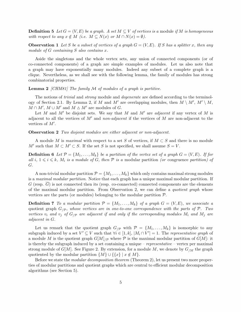
Let us remark that the quotient graph G/P with P = {M1, . . . ,Mk} is isomorphic to anysubgraph induced by a set V ′ ⊆ V such that ∀i ∈ [1, k], |Mi ∩ V ′| = 1. The representative graph ofa module M is the quotient graph G[M ]/P where P is the maximal modular partition of G[M ]: itis thereby the subgraph induced by a set containing a unique – representative – vertex per maximalstrong module of G[M ]. See Figure 2. By extension, for a module M , we denote by G/M the graphquotiented by the modular partition {M} ∪ {{x} | x /∈M}.

Before we state the modular decomposition theorem (Theorem 2), let us present two more proper-ties of modular partitions and quotient graphs which are central to efficient modular decompositionalgorithms (see Section 5).

5

16

7

89

1011

4

2

3

5

9

103

45

61

Figure 2: On the left, the grey sets are modules of the graph G. Q ={{1}, {2, 3}, {4}, {5}, {6, 7}, {9}, {8, 10, 11}} is a modular partition of G. The quotient graphG/Q, depicted on the right with a representative vertex for each module of Q, has two non-trivial modules (the sets {3, 4} and {9, 10}). The maximal modular partition of G is P ={{1}, {2, 3, 4}, {5}, {6, 7}, {8, 9, 10, 11}} and its quotient graph are represented in Figure 3 (asidethe top node of the tree).

Lemma 3 [Moh85b] Let P be a modular partition of a graph G = (V,E). Then X ⊆ P is a moduleof G/P iff

⋃M∈X M is a module of G.

Lemma 3 is illustrated on Figure 2: for example, the set {2, 3, 4} is a module of G, it is the unionof modules {2, 3} and {4} (which representative vertices are respectively 3 and 4 in G/Q) whichbelongs to partition Q. It can be strengthened in order to observe the correspondance between thestrong modules of G and those of G/P .

Lemma 4 Let P be a modular partition of a graph G = (V,E). Then X ⊂ P is a non-trivialstrong module of G/P iff

⋃M∈X M is a non trivial strong module of G.

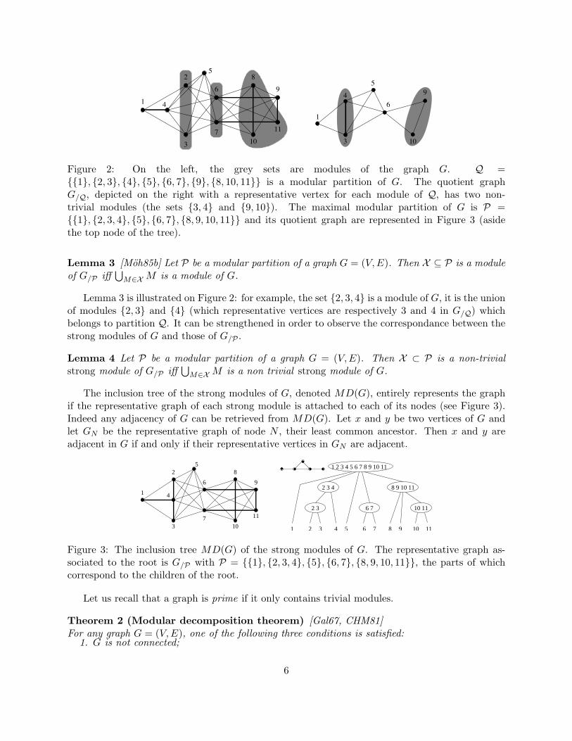
The inclusion tree of the strong modules of G, denoted MD(G), entirely represents the graphif the representative graph of each strong module is attached to each of its nodes (see Figure 3).Indeed any adjacency of G can be retrieved from MD(G). Let x and y be two vertices of G andlet GN be the representative graph of node N , their least common ancestor. Then x and y areadjacent in G if and only if their representative vertices in GN are adjacent.

1 2 3 4 5 6 7 8 9 10 11��

1

2

3

4

5

6

7

8

9

10

11

1 9852 43 6 7 1110

8 9 10 11

2 3

2 3 4

6 7 10 11

�

Figure 3: The inclusion tree MD(G) of the strong modules of G. The representative graph as-sociated to the root is G/P with P = {{1}, {2, 3, 4}, {5}, {6, 7}, {8, 9, 10, 11}}, the parts of whichcorrespond to the children of the root.

Let us recall that a graph is prime if it only contains trivial modules.

Theorem 2 (Modular decomposition theorem) [Gal67, CHM81]For any graph G = (V,E), one of the following three conditions is satisfied:

1. G is not connected;

6

2. G is not connected;

3. G and G are connected and the quotient graph G/P , with P the maximal modular partitionof G, is a prime graph.

What does the modular decomposition theorem say is twofold. First, the quotient graphsassociated with the nodes of the inclusion tree MD(G) of the strong modules are of three types:an independent set if G is not connected (the node is labelled parallel); a clique (complete graph)if G is not connected (the node is labelled series); a prime graph otherwise. It also follows thatMD(G) is unique and does not contain two consecutive series nodes nor two consecutive parallelnodes. Parallel and series nodes of MD(G) are also called degenerate nodes.

The tree MD(G) is called the modular decomposition tree. Theorem 2 yields a natural poly-nomial time recursive algorithm to compute MD(G): 1) compute the maximal modular partitionP of G; 2) label the root node according to the parallel, series or prime type of G; 3) for eachmodule M of P, compute MD(G[M ]) and attach it to the root node. A subproblem central tothe computation of MD(G) is to compute the maximal modular partition, a task which can beavoided if a non-trivial module M is identified. This yields another natural algorithm scheme: byLemma 3 and Lemma 4, it suffices to recursively compute MD(G[M ]) and MD(G/M ), and thento paste MD(G[M ]) on the leaf of MD(G/M ) corresponding to the representative vertex of M . Assuggested by Cowan et al. [CJS72], a naive way to compute a non-trivial module is to follow thedefinition of module and Observation 1. Assume the graph G contains a non-trivial module M .Then M contains a pair of vertices {x, y} and as a module is closed under adding splitters. Suchan algorithm would find a non-trivial module, if any, in time O(n2(n+m)). We should note thatfor some generalizations of the modular decomposition, no better algorithm than this ”closure bysplitter” approach is known (see e.g. [BXHLdM09]).

Before we present some structural properties of prime and totally decomposable graphs, letus introduce some notations and briefly discuss the composition view of the theory of modules ingraphs.

Notation 3 For a node p of MD(G), its corresponding strong module is denoted by M(p) (or P ).In fact M(p) is the union of all singletons which are leaves of the subtree of M(p) rooted in p.The minimal strong module containing two vertices x and y is denoted by m(x, y), while the maximalstrong module containing x but not y, for any two different vertices x, y of G, is denoted by M(x, y).

The substitution operation is the reverse of the quotient operation. It consists of replacing avertex x of G by a graph H = (V ′, E′) while preserving the neighourhood. The resulting graph is:

Gx→H = ((V \ {x}) ∪ V ′, (E \ {xy ∈ E}) ∪ E′ ∪ {yz : xy ∈ E et z ∈ V ′})

The parallel composition or disjoint union of k connected graphs G1, . . . Gk defines a graphwhose connected components are the graphs G1, . . . , Gk. This composition operation is usuallydenoted G1 ⊕ · · · ⊕Gk.

The series composition of k co-connected graphs G1, . . . , Gk defines a graph whose co-connectedcomponents are the graphs G1, . . . , Gk (for any pair x, y of vertices belonging to different graphs Gi

and Gj , the edge xy has been added). The series composition is generally denoted G1 ⊗ · · · ⊗Gk.These three operations are classical graph operations that have been widely used in various

contexts among which the clique-width theory [CER93].

7

2.4 Prime graphs

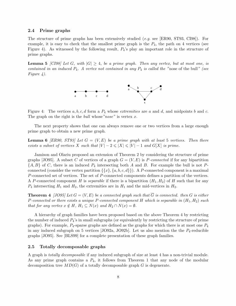
The structure of prime graphs has been extensively studied (e.g. see [ER90, ST93, CI98]). Forexample, it is easy to check that the smallest prime graph is the P4, the path on 4 vertices (seeFigure 4). As witnessed by the following result, P4’s play an important role in the structure ofprime graphs.

Lemma 5 [CI98] Let G, with |G| ≥ 4, be a prime graph. Then any vertex, but at most one, iscontained in an induced P4. A vertex not contained in any P4 is called the ”nose of the bull” (seeFigure 4).

c

��

��

��

��

��

��

��

��

��

��

��

��

x

b c da

b da

��

Figure 4: The vertices a, b, c, d form a P4 whose extremities are a and d, and midpoints b and c.The graph on the right is the bull whose”nose” is vertex x.

The next property shows that one can always remove one or two vertices from a large enoughprime graph to obtain a new prime graph.

Lemma 6 [ER90, ST93] Let G = (V,E) be a prime graph with at least 5 vertices. Then thereexists a subset of vertices X such that |V | − 2 6 |X| 6 |V | − 1 and G[X] is prime.

Jamison and Olariu proposed an extension of Theorem 2 by considering the structure of primegraphs [JO95]. A subset C of vertices of a graph G = (V,E) is P -connected if for any bipartition{A,B} of C, there is an induced P4 intersecting both A and B. For example the bull is not P -connected (consider the vertex partition {{x}, {a, b, c, d}}). A P -connected component is a maximalP -connected set of vertices. The set of P -connected components defines a partition of the vertices.A P -connected component H is separable if there is a bipartition (H1, H2) of H such that for anyP4 intersecting H1 and H2, the extremities are in H1 and the mid-vertices in H2.

Theorem 4 [JO95] Let G = (V,E) be a connected graph such that G is connected. then G is eitherP -connected or there exists a unique P -connected component H which is separable in (H1, H2) suchthat for any vertex x /∈ H, H1 ⊆ N(x) and H2 ∩N(x) = ∅.

A hierarchy of graph families have been proposed based on the above Theorem 4 by restrictingthe number of induced P4’s in small subgraphs (or equivalently by restricting the structure of primegraphs). For example, P4-sparse graphs are defined as the graphs for which there is at most one P4

in any induced subgraph on 5 vertices [JO92a, JO92b]. Let us also mention the the P4-reduciblegraphs [JO95]. See [BLS99] for a complete presentation of these graph families.

2.5 Totally decomposable graphs

A graph is totally decomposable if any induced subgraph of size at least 4 has a non-trivial module.As any prime graph contains a P4, it follows from Theorem 1 that any node of the modulardecomposition tree MD(G) of a totally decomposable graph G is degenerate.

8

The family F of totally decomposable graphs is natural and arose in many different contexts (see[Sum73, CLSB81, CPS85] for references) even recently (see [BBCP04, BRV07]) as any graph of Fcan be obtained by a sequence of disjoint and series compositions starting from single vertex graph.Let us remark that if G is totally decomposable then also is its complement. The family of totallydecomposable graphs is also known as the cographs for complement reducible graphs [CLSB81,Sum73]. From definition, the cograph family is hereditary (any induced subgraph of a cograph is acograph). It also has a very simple forbidden subgraph characterization.

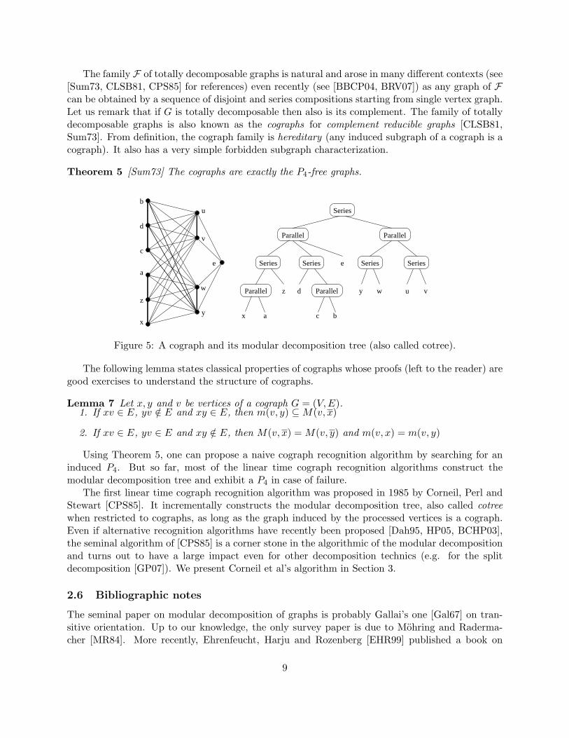
Theorem 5 [Sum73] The cographs are exactly the P4-free graphs.

e

b

c

d

u

v

a

z

yx

w

Parallel

Series

Series Series Series Series

Parallel

ParallelParallel d wy u

e

z

ax

v

c b

Figure 5: A cograph and its modular decomposition tree (also called cotree).

The following lemma states classical properties of cographs whose proofs (left to the reader) aregood exercises to understand the structure of cographs.

Lemma 7 Let x, y and v be vertices of a cograph G = (V,E).1. If xv ∈ E, yv /∈ E and xy ∈ E, then m(v, y) ⊆M(v, x)

2. If xv ∈ E, yv ∈ E and xy /∈ E, then M(v, x) = M(v, y) and m(v, x) = m(v, y)

Using Theorem 5, one can propose a naive cograph recognition algorithm by searching for aninduced P4. But so far, most of the linear time cograph recognition algorithms construct themodular decomposition tree and exhibit a P4 in case of failure.

The first linear time cograph recognition algorithm was proposed in 1985 by Corneil, Perl andStewart [CPS85]. It incrementally constructs the modular decomposition tree, also called cotreewhen restricted to cographs, as long as the graph induced by the processed vertices is a cograph.Even if alternative recognition algorithms have recently been proposed [Dah95, HP05, BCHP03],the seminal algorithm of [CPS85] is a corner stone in the algorithmic of the modular decompositionand turns out to have a large impact even for other decomposition technics (e.g. for the splitdecomposition [GP07]). We present Corneil et al’s algorithm in Section 3.

2.6 Bibliographic notes

The seminal paper on modular decomposition of graphs is probably Gallai’s one [Gal67] on tran-sitive orientation. Up to our knowledge, the only survey paper is due to Mohring and Raderma-cher [MR84]. More recently, Ehrenfeucht, Harju and Rozenberg [EHR99] published a book on

9

the decomposition of 2-structures (a generalization of graphs) which presents the modular decom-position in a more general framework. In its PhD thesis [BX08], Bui Xuan proposes a surveyas well as original results on the representation of set families. Many graph families are well-structured with respect to the modular decomposition, e.g. comparability graphs, permutationgraphs, cographs. . . For these aspects, the reader should refer to the books of Golumbic [Gol80] andmore recently [BLS99, Spi03]. The algorithmic aspects are particularly developed in [Gol80, Spi03].

We saw that the family of modules in a graph is partitive. If we move to directed graphs,then we obtain a weakly partitive family. The related decomposition of bipartite graph into bi-modules also yields a weakly parititive family [FHdMV04]. In order to formalize split decomposition[CE80], bipartitive families have been introduced [CE80, Cun82]. For a recent survey on all kindof variations on the modular decomposition, the reader should refer to [BX08].

3 Cographs recognition algorithms as an appetizer

We first study in detail the Corneil, Pearl and Stewart’s algorithm [CPS85]. If the input graph isa cograph, this vertex-incremental algorithm builds the cotree by adding the vertices one by onein an arbitrary order. Then, we sketch how the cotree of a cograph can be updated under edgemodification, a result is due to Shamir and Sharan [SS04].

3.1 Adding a vertex to a cograph

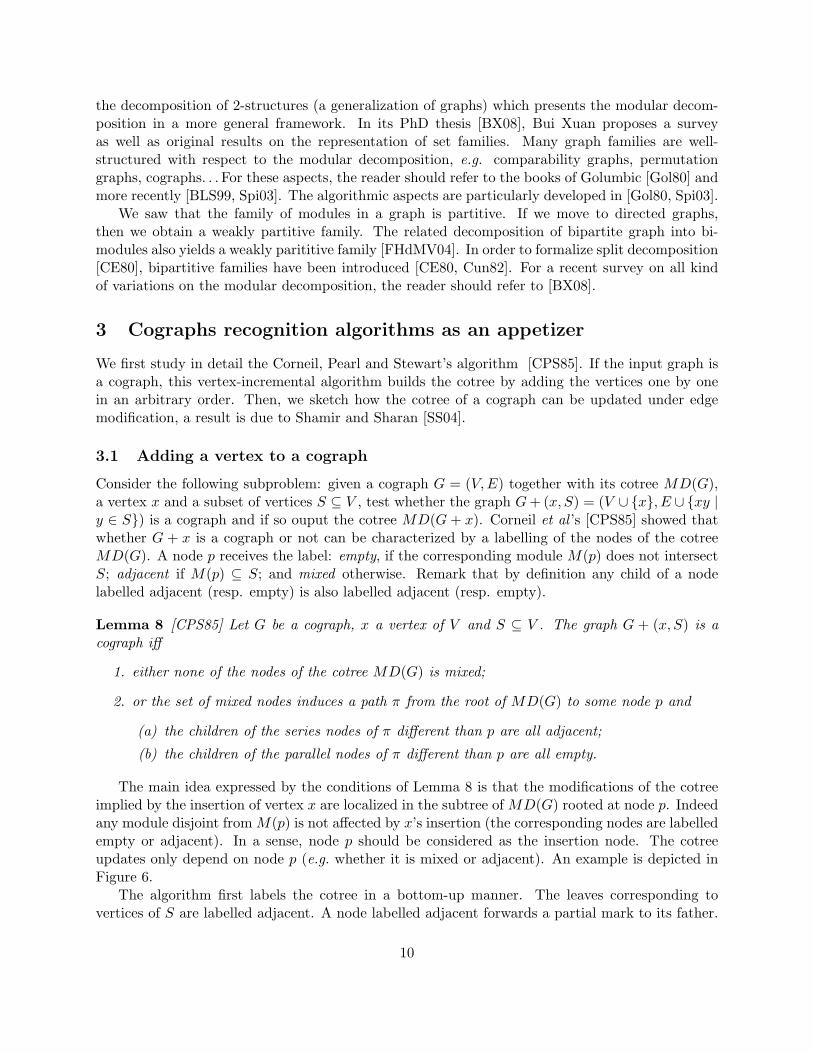
Consider the following subproblem: given a cograph G = (V,E) together with its cotree MD(G),a vertex x and a subset of vertices S ⊆ V , test whether the graph G+ (x, S) = (V ∪ {x}, E ∪ {xy |y ∈ S}) is a cograph and if so ouput the cotree MD(G+ x). Corneil et al ’s [CPS85] showed thatwhether G + x is a cograph or not can be characterized by a labelling of the nodes of the cotreeMD(G). A node p receives the label: empty, if the corresponding module M(p) does not intersectS; adjacent if M(p) ⊆ S; and mixed otherwise. Remark that by definition any child of a nodelabelled adjacent (resp. empty) is also labelled adjacent (resp. empty).

Lemma 8 [CPS85] Let G be a cograph, x a vertex of V and S ⊆ V . The graph G + (x, S) is acograph iff

1. either none of the nodes of the cotree MD(G) is mixed;

2. or the set of mixed nodes induces a path π from the root of MD(G) to some node p and

(a) the children of the series nodes of π different than p are all adjacent;

(b) the children of the parallel nodes of π different than p are all empty.

The main idea expressed by the conditions of Lemma 8 is that the modifications of the cotreeimplied by the insertion of vertex x are localized in the subtree of MD(G) rooted at node p. Indeedany module disjoint from M(p) is not affected by x’s insertion (the corresponding nodes are labelledempty or adjacent). In a sense, node p should be considered as the insertion node. The cotreeupdates only depend on node p (e.g. whether it is mixed or adjacent). An example is depicted inFigure 6.

The algorithm first labels the cotree in a bottom-up manner. The leaves corresponding tovertices of S are labelled adjacent. A node labelled adjacent forwards a partial mark to its father.

10

��

��

��

��

��

��

��

��

��

Series

f

Series

Series

��

Series

Parallel ParallelG+x

a b c d e f

��

��

x

a c

b d e��

g h

g h

Parallel

Parallel Parallel

SeriesSeries

Series

Figure 6: Insertion of the vertex x adjacent to S = {b, d, g, h}. Grey nodes are the adjacent labellednodes and dashed nodes are the mixed nodes. The insertion node p is the bold series node (fatherof a, b, c, d).

When a node have received a mark from each of its children, it is labelled adjacent. At the end of thisprocess the empty node have never been searched, while the partially marked nodes corresponds,if G + x is a cograph, to the parallel nodes of the path π from the insertion node to the root ofMD(G). It is not difficult to see that the number of the marked nodes is linear in the size of Smeaning that the labelling process runs in time O(|S|). Testing the condition of the above lemmacan be done within the same complexity as well.

Theorem 6 [CPS85] The family of cographs can be recognized in linear time.

3.2 Edge modification algorithms for cographs

Let us now turn to the edge modification problem which consists in updating the cotree of a cographG under an edge insertion or deletion. Since the cotree of a cograph can be obtained from the cotreeof its complement by flipping the parallel and the series nodes, deleting or inserting an edge in acograph are equivalent problems.

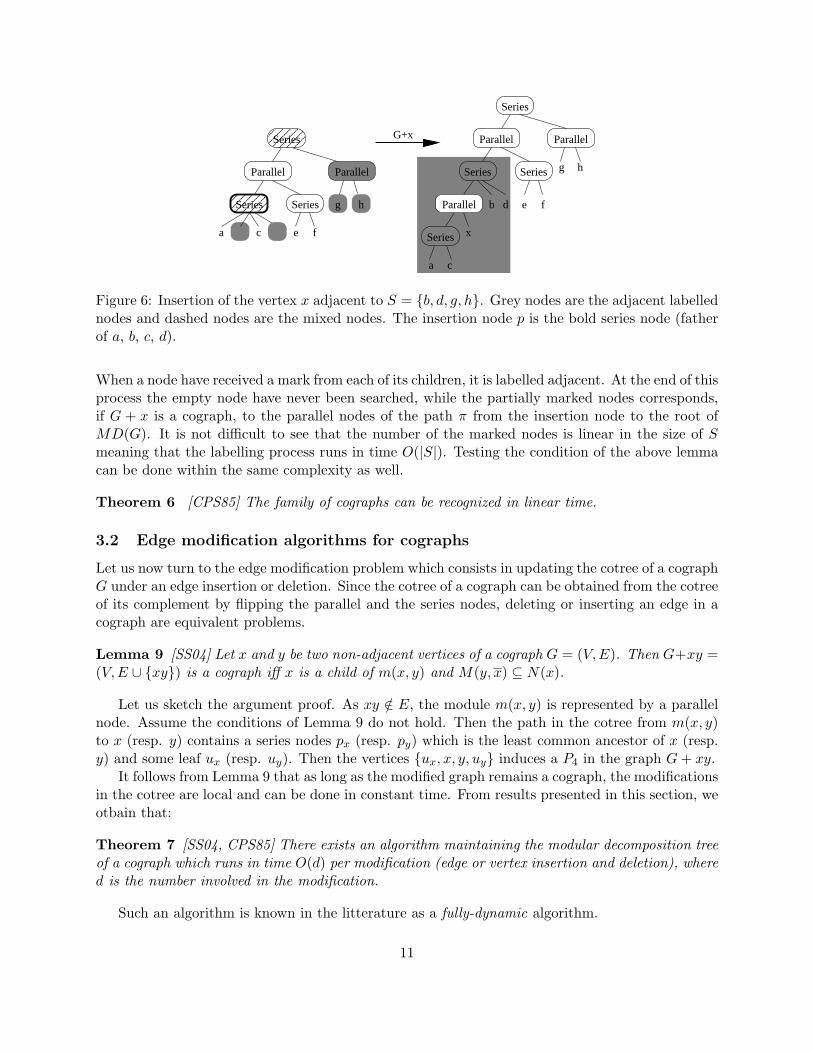
Lemma 9 [SS04] Let x and y be two non-adjacent vertices of a cograph G = (V,E). Then G+xy =(V,E ∪ {xy}) is a cograph iff x is a child of m(x, y) and M(y, x) ⊆ N(x).

Let us sketch the argument proof. As xy /∈ E, the module m(x, y) is represented by a parallelnode. Assume the conditions of Lemma 9 do not hold. Then the path in the cotree from m(x, y)to x (resp. y) contains a series nodes px (resp. py) which is the least common ancestor of x (resp.y) and some leaf ux (resp. uy). Then the vertices {ux, x, y, uy} induces a P4 in the graph G+ xy.

It follows from Lemma 9 that as long as the modified graph remains a cograph, the modificationsin the cotree are local and can be done in constant time. From results presented in this section, weotbain that:

Theorem 7 [SS04, CPS85] There exists an algorithm maintaining the modular decomposition treeof a cograph which runs in time O(d) per modification (edge or vertex insertion and deletion), whered is the number involved in the modification.

Such an algorithm is known in the litterature as a fully-dynamic algorithm.

11

p

m(x,y)

q

��

��

c

��

��

��

��

Series

Series

Series

ParallelG+xy

a b c

a

��

b

ySeries

Parallel Parallel

Series

x d e f

e f

xy

Parallel

Parallel

d

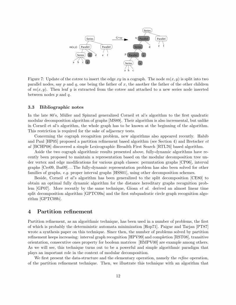
Figure 7: Update of the cotree to insert the edge xy in a cograph. The node m(x, y) is split into twoparallel nodes, say p and q, one being the father of x, the another the father of the other childrenof m(x, y). Then leaf y is extracted from the cotree and attached to a new series node insertedbetween nodes p and q.


In the late 80’s, Muller and Spinrad generalized Corneil et al’s algorithm to the first quadraticmodular decomposition algorithm of graphs [MS89]. Their algorithm is also incremental, but unlikein Corneil et al’s algorithm, the whole graph has to be known at the beginning of the algorithm.This restriction is required for the sake of adjacency tests.

Concerning the cograph recognition problem, new algorithms also appeared recently. Habiband Paul [HP05] proposed a partition refinement based algorithm (see Section 4) and Bretscher etal [BCHP08] discovered a simple Lexicographic Breadth First Search [RTL76] based algorithm.

Aside the two cograph algorithmic results presented above, fully-dynamic algorithms have re-cently been proposed to maintain a representation based on the modular decomposition tree un-der vertex and edge modifications for various graph classes: permutation graphs [CP06], intervalgraphs [Cre09, Iba09]. . . The fully-dynamic representation problem has also been solved for otherfamilies of graphs, e.g. proper interval graphs [HSS01], using other decomposition schemes.

Beside, Corneil et al ’s algorithm has been generalized to the split decomposition [CE80] toobtain an optimal fully dynamic algorithm for the distance hereditary graphs recognition prob-lem [GP07]. More recently by the same technique, Gioan et al. derived an almost linear timesplit decomposition algorithm [GPTC09a] and the first subquadratic circle graph recognition algo-rithm [GPTC09b].

4 Partition refinement

Partition refinement, as an algorithmic technique, has been used in a number of problems, the firstof which is probably the deterministic automata minimization [Hop71]. Paigue and Tarjan [PT87]wrote a synthesis paper on this technique. Since then, the number of problems solved by partitionrefinement keeps increasing: interval graph recognition [HPV99] and completion [RST08], transitiveorientation, consecutive ones property for boolean matrices [HMPV00] are example among others.As we will see, this technique turns out to be a powerful and simple algorithmic paradigm thatplays an important role in the context of modular decomposition.

We first present the data-structure and the elementary operation, namely the refine operation,of the partition refinement technique. Then, we illustrate this technique with an algorithm that

12

computes a modular partition of a graph. Let us mention that this algorithm really follows thelines of Hopcroft’s deterministic automaton minimization algorithm [Hop71].

4.1 Data-structures and algorithmic scheme

Let P and P ′ be two partitions of the same set V . The partition P is smaller than P ′, denotedP / P ′, if P 6= P ′ and any part of P is a subset of some part of P ′. The partition P is stable withrespect to a set S if none of the parts of P overlaps S.

Partition refinement consists of repeating, as long as needed, the operation described in Al-gorithm 1. The initial partition and the sequence of pivot sets used in the successive refinementsteps have a large impact on the whole complexity of the algorithm. Partitioning the vertex setof a graph with respect to the neighbourhood of some vertex is a common operation in graphalgorithms. Indeed in our examples, all pivot sets considered correspond to the neighbourhood ofsome vertex.

Algorithm 1: Refine(P, S)Input: A partition P of a set V and a subset S ⊆ V , called pivot setOutput: The coarsest partition refining P and stable for Sbegin

foreach part X ∈ P doif X ∩ S 6= ∅ and X ∩ S 6= X then replace X by X ∩ S and X \ S;

end

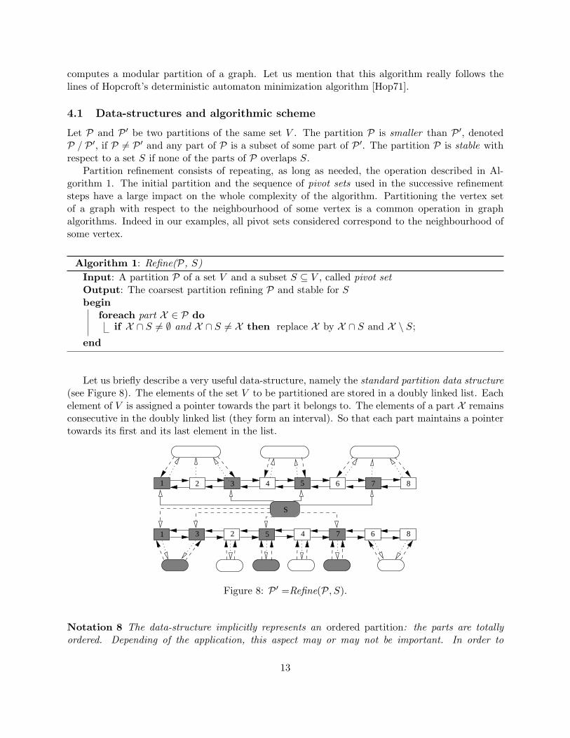
Let us briefly describe a very useful data-structure, namely the standard partition data structure(see Figure 8). The elements of the set V to be partitioned are stored in a doubly linked list. Eachelement of V is assigned a pointer towards the part it belongs to. The elements of a part X remainsconsecutive in the doubly linked list (they form an interval). So that each part maintains a pointertowards its first and its last element in the list.

1

4 6 8

53 8

S

2 4 6 7

75231

Figure 8: P ′ =Refine(P, S).

Notation 8 The data-structure implicitly represents an ordered partition: the parts are totallyordered. Depending of the application, this aspect may or may not be important. In order to

13

distinguish the two different cases, an ordered partition will be denoted by P = [X1, . . . ,Xk] while anon-ordered partition will be denoted by P = {X1, . . . ,Xk}.

Given a subset S ⊆ V , using this standard partition data structure, one can build a list Lcontaining the parts of P intersecting S, such that in each of these parts the elements of S occurfirst. Then using L, one can split every part into X ∩ S and X \ S. A careful complexity analysisshows the following result:

Lemma 10 The time complexity of the operation Refine(P, S) is O(|S|).

We conclude this brief introduction by a few remarks. Refining a partition by a subset S orits complement S = V \ S are equivalent operations: Refine(X , S)= Refine(X ∩ S, V \ S). Itis thereby possible to deal with the complement of the input graph without explicitly storing itsedge set. Partition refinement is usually used either to compute a total ordering of the vertices(e.g. LexBFS) or the equivalence classes of some equivalence relations (e.g. maximal set of twinvertices). McConnell and Spinrad [MS00] showed how to augment the data-structure in orderto extract within the same complexity, at each refinement step, the edges incident to verticesbelonging to different parts. This operation is useful to efficiently compute the quotient graphassociated to a modular partition. For a more detailed presentation of partition refinement referto [PT87, HPV98, HPV99, HMPV00].

Of course many variations of the standard partition data structure have been introduced, asfor example changing the doubly linked list into an array of size |V |. A further requirement canbe that the elements of every part X of P are maintained sorted according to a given an initialordering τ of V . This can be done within the same complexity and is very useful for example whendealing with LexBFS multi-sweep algorithms. The ordering given by some previous LexBFS canbe used as a tie-break rule for another LexBFS [Cor04b, Cor04a, BCHP08].

4.2 Hopcroft’s rule and computation of a modular partition

Partition refinement is the right tool to compute a modular partition, an important subproblemtowards efficient modular decomposition algorithms. In this section, we focus on the problemof computing the coarsest modular partition (see Definition 8) of a given vertex partition. Thealgorithm we present runs in time O(n+m log n) and is based on the Hopcroft’s rule which is usedin various simple quasi-linear time modular decomposition algorithms.

Definition 8 Let P be a partition of the vertices of a graph G = (V,E). The coarsest modularpartition of G with respect to P is the largest modular partition Q such that Q / P.

The main idea of the algorithm is the following: as long as there is a part X which is not uniformfor some vertex x /∈ X , the current partition P is refined with the neighbourhood N(x). When thealgorithm ends, all the parts are modules. Finding, at each step, a vertex x whose neighbourhoodstrictly refines the partition P, is the usual barrier to linear time complexity. However, using theso-called Hopcroft’s rule, one get a fairly simple solution that uses the neighbourhood of each vertexat most log n times.

Lemma 11 Let P be a partition of the vertices of a graph G = (V,E) and x be a vertex of somepart X . If P is stable with respect to N(y), ∀y /∈ X , then X is a module of G and the partitionQ = Refine(P, N(x)) is stable with respect to N(x′), ∀x′ ∈ X .

14

The above lemma (which is a direct consequence of the definition of module) shows that usingas pivots the vertices of all the parts of P but one, say Z, plus one vertex z of Z is enough. Forcomplexity issues, the avoided part Z has to be chosen as the largest part of P. Similarly, oncea part X has been split, the process continues recursively on the subgraph induced by X and theresulting largest subpart can be avoided (meaning that only one of its vertices has to be used aspivot). This ”avoid the largest part” technique is known as the Hopcroft’s rule and has been firstproposed in the deterministic automata minimization algorithm [Hop71].

Algorithm 2: Modular PartitionInput: A partition P of the vertex set V of a graph GOutput: The coarsest modular partition Q smaller than Pbegin

Let Z be the largest part of P;Q ← P; K ← {Z}; L← {X | X 6= Z,X ∈ P};while L ∪K 6= ∅ do1

if there exists X ∈ L then S ← X and L← L \ {X};else

Let X be the first part K and x arbitrarily selected in X ;2

S ← {x} and K ← K \ {X};foreach vertex x ∈ S do

foreach part Y 6= X such that N(x) ⊥ Y doReplace in Q, Y by Y1 = Y ∩N(x) and Y2 = Y \N(x);3

Let Ymin (resp. Ymax) be the smallest part (resp. largest) among Y1 and Y2;if Y ∈ L then L← L ∪ {Ymin,Ymax} \ {Y};else

L← L ∪ {Ymin};if Y ∈ K then Replace Y by Ymax in K;else Add Ymax at the end of K;

end

To implement this rule, the parts are stored in two disjoint lists K and L. The neighbourhoodsof all the vertices of parts belonging to L will be used to refine the partition. For the parts belongingto K, only the neighbourhood of one arbitrarily selected vertex is used. Since K is managed witha FIFO priority rule, this guarantees that the first part of the list, when extracted, is a module.

Theorem 9 Let P be a partition of the vertices of a graph G = (V,E). Algorithm 2 computes thecoarsest modular partition for G and P in time O(n+m log n).

The correctness of the algorithm follows from the next three invariant properties. The firstinvariant shows that a module contains in some part of the given partition cannot be split, whilethe third one guarantees that the algorithm outputs a modular partition.

1. If M is a module of G contained in a part X ∈ P, then there exists a part Y of the currentpartition containing M .

2. If L = ∅, then the first part Y of K is a module.

15

3. If the current partition contains a part X that is not a module, then there exists Y ∈ L ∪Kdifferent from X and containing a splitter y for X .

Complexity issues: The main while loop (line 2), manages a set S of vertices whose neighbourhoodshave to be used to refine the current partition. The set S is computed from the lists L and K.Since the current part containing a given vertex can be added to L, only if its size is smaller thanhalf of the size of the former part containing x, the neighbourhood of each vertex x is guaranteedto be visited at most log(|V |) times by the algorithm. Furthermore, when a vertex x of a part Xextracted from K is used, neither x nor none of the vertices of X is used again. This yields to aO(

∑x∈V log(|V |).|N(x)|) complexity, as claimed.


As already mentioned, the use of partition refinement technique dates to 1971 for the determinis-tic automata minimization problem [Hop71]. In 1987, Paigue and Tarjan used again this technicto solve three different problems: functional partition, coarsest relational partition problems anddoubly lexicographic ordering of a boolean matrix. In the late 90’s, it has been used more system-atically in the context of modular decomposition and transitive orientation yielding O(n+m log n)practical and simple algorithms (see e.g. [MS00, HMPV00]).

5 Recursive computation of the modular decomposition tree

In 1994, Ehrenfeucht, Gabow, McConnell and Sullivan [EGMS94] proposed a quadratic algorithmfor the modular decomposition1. The principle of this algorithm, which we will call the skeletonalgorithm, is the basis of a large number of the known subquadratic algorithms proposed in thelate 90’s (see e.g. [MS00, DGM01]), which could abusively be considered as a series of differentimplementations of the skeleton algorithm. The complexity of these implementations are respec-tively O(n + m.α(n,m)) or O(n + m) [DGM01], and finally O(n + m log n) [MS00]. We describethe principle of the skeleton algorithm without considering the complexity issues. We then discussthe differences in the time complexity of the known algorithms.

5.1 The skeleton algorithm

Let us first mention that the skeleton algorithm computes a non-reduced form of the modulardecomposition tree MD(G): the resulting tree may contain some series (or parallel) node child ofa series (or parallel) node. All the algorithms we describe in this section will do so. It does notimpact the complexity issues as a single search of the tree is enough reduce it in time O(n). Inthe following, we will abusively denote MD(G) the (non-reduced) decomposition tree returned bythese algorithms.

The main idea developed by Ehrenfeucht et al. [EGMS94] is to first compute a ”spine” of themodular decomposition tree MD(G), then to recursively compute the modular decomposition treesof some induced subgraphs which are eventually padded to the spine. More formally:

1This algorithm is designed for 2-structures, a classical generalization of graphs.

16

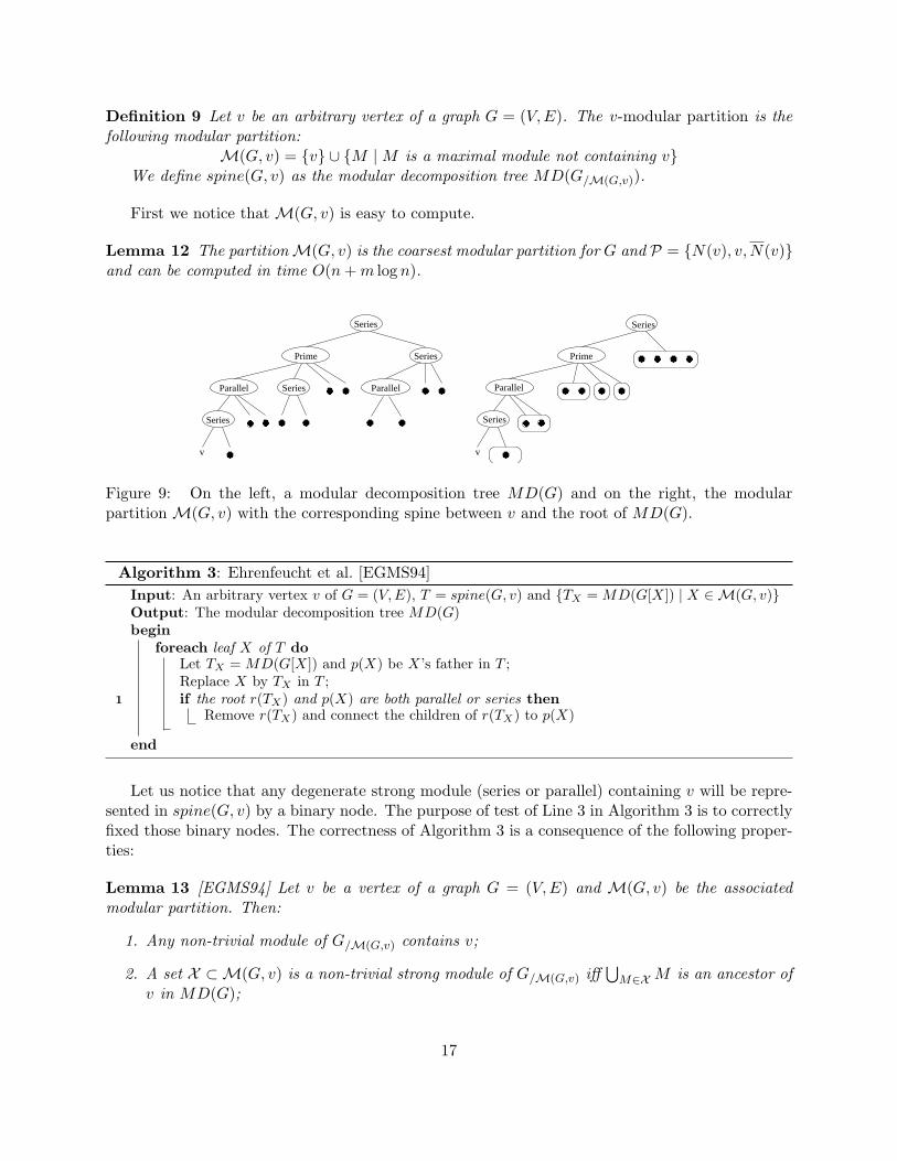
Definition 9 Let v be an arbitrary vertex of a graph G = (V,E). The v-modular partition is thefollowing modular partition:

M(G, v) = {v} ∪ {M |M is a maximal module not containing v}We define spine(G, v) as the modular decomposition tree MD(G/M(G,v)).

First we notice that M(G, v) is easy to compute.

Lemma 12 The partitionM(G, v) is the coarsest modular partition for G and P = {N(v), v,N(v)}and can be computed in time O(n+m log n).

Series

��

��

��

��

��

��

��

��

��

��

��

Parallel

Prime

v v

Series

Series

Series

Series

Parallel

Series

Parallel

Prime

Figure 9: On the left, a modular decomposition tree MD(G) and on the right, the modularpartition M(G, v) with the corresponding spine between v and the root of MD(G).

Algorithm 3: Ehrenfeucht et al. [EGMS94]Input: An arbitrary vertex v of G = (V,E), T = spine(G, v) and {TX = MD(G[X]) | X ∈M(G, v)}Output: The modular decomposition tree MD(G)begin

foreach leaf X of T doLet TX = MD(G[X]) and p(X) be X’s father in T ;Replace X by TX in T ;if the root r(TX) and p(X) are both parallel or series then1

Remove r(TX) and connect the children of r(TX) to p(X)

end

Let us notice that any degenerate strong module (series or parallel) containing v will be repre-sented in spine(G, v) by a binary node. The purpose of test of Line 3 in Algorithm 3 is to correctlyfixed those binary nodes. The correctness of Algorithm 3 is a consequence of the following proper-ties:

Lemma 13 [EGMS94] Let v be a vertex of a graph G = (V,E) and M(G, v) be the associatedmodular partition. Then:

1. Any non-trivial module of G/M(G,v) contains v;

2. A set X ⊂M(G, v) is a non-trivial strong module of G/M(G,v) iff⋃

M∈X M is an ancestor ofv in MD(G);

17

3. Any module not containing v is a subset of a part M ∈M(G, v).

Computing spine(G, v) is a the difficult and technical task of the skeleton algorithm, indeed it isits main complexity bottleneck. The solution we present hereafter has been proposed in [EGMS94]and yields quadratic running time. Later on, Dahlhaus et al. [DGM01] improved this step andobtained a subquadratic running time (see discussion of Section 5.3).

5.2 Computation of spine(G, v).

Definition 10 A graph G = (V,E) is nested if there exists a vertex v ∈ V which is contained inall the non-trivial modules of G. Such a vertex is called an inner vertex of G.

As a direct consequence of Lemma 13, the quotient graph G/M(G,v) is a nested graph with innervertex v.

In order to compute the modules of G/M(G,v) and spine(G, v), Ehrenfeucht et al. [EGMS94]introduced an auxiliary forcing digraph the arc set of which guarantees the existence of a directedpath from any vertex u to any vertex w ∈ m(u, v), the smallest module containing u and v. As vbelongs to all the modules of G/M(G,v), a simple search on the forcing graph will suffice to computespine(G, v).

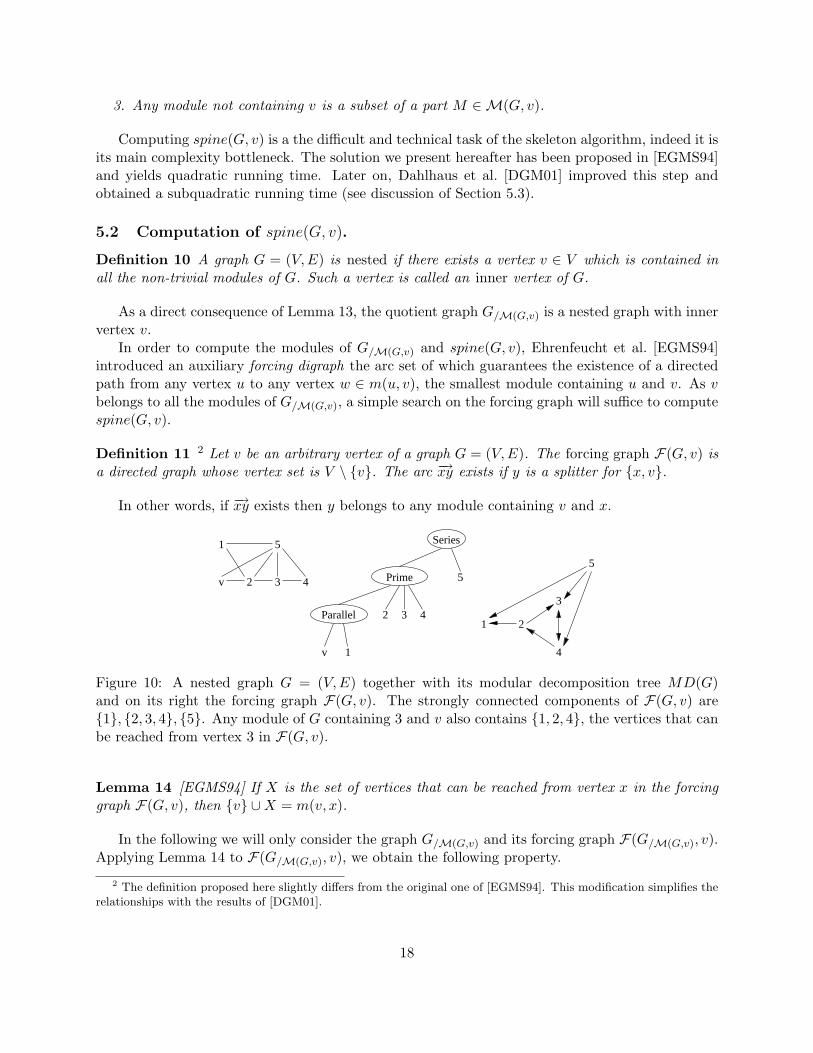
Definition 11 2 Let v be an arbitrary vertex of a graph G = (V,E). The forcing graph F(G, v) isa directed graph whose vertex set is V \ {v}. The arc −→xy exists if y is a splitter for {x, v}.

In other words, if −→xy exists then y belongs to any module containing v and x.

2

v

1 5

2 3 4

1 2

5

3

4

Series

Prime

Parallel 3 4

5

1v

Figure 10: A nested graph G = (V,E) together with its modular decomposition tree MD(G)and on its right the forcing graph F(G, v). The strongly connected components of F(G, v) are{1}, {2, 3, 4}, {5}. Any module of G containing 3 and v also contains {1, 2, 4}, the vertices that canbe reached from vertex 3 in F(G, v).

Lemma 14 [EGMS94] If X is the set of vertices that can be reached from vertex x in the forcinggraph F(G, v), then {v} ∪X = m(v, x).

In the following we will only consider the graph G/M(G,v) and its forcing graph F(G/M(G,v), v).Applying Lemma 14 to F(G/M(G,v), v), we obtain the following property.

2 The definition proposed here slightly differs from the original one of [EGMS94]. This modification simplifies therelationships with the results of [DGM01].

18

Corollary 1 [EGMS94] Let Mx be the module of M(G, v) containing the vertex x. If X is the setof modules that can be reached from Mx in F(G/M(G,v), v), then

⋃M∈X M = m(v, x).

We now consider the block graph B(G, v) of F(G/M(G,v), v) (see [CLR90]) whose vertices arethe strongly connected components of F(G/M(G,v), v), also called the blocks of (G, v). An arc ofB(G, v) between the block B and B′ exists if the vertices of B′ can be reached in F(G/M(G,v), v)from the vertices of B.

Lemma 15 [EGMS94] The transitive reduction of the block graph B(G, v) is a chain.

A set of vertices of a digraph is a sink if it has no out-neighbour. By Lemma 15, any sink set ofF(M(G, v)) is the union of consecutive blocks containing the last one in the transitive reductionof B(G, v). Each sink set corresponds to a module of G/M(G,v).

Corollary 2 [EGMS94] Let v be a vertex of a graph G = (V,E). A set M of vertices containing vis a module of G/M(G,v) iff M is the union of {v} and the modules of M(G, v) belonging to a sinkset X of B(G, v).

Thereby the forcing graph F(G/M(G,v), v) describes the modules of G/M(G,v) and the blockgraph B(G, v) allows us to compute spine(G, v). Finally, MD(G) is obtained recursively by follow-ing the lines of Lemma 13.

5.3 Complexity issues

Rather than detailing the complexity analysis, we point out the differences between the originalskeleton algorithm presented in [EGMS94] and its later versions improved in [DGM01]. The inter-ested reader should access the original papers for details. As already mentioned, a quadratic timecomplexity analysis is proposed in [EGMS94]. The main bottlenecks are the computation of thepartition M(G, v) and the construction of MD(G/M(G,v)).

Two new versions of the skeleton algorithm proposed by Dahlhaus, Gustedt and McConnell [DGM01],respectively run in O(n + m.α(n,m)) time and in linear time. To improve the time complexity,the authors of [DGM01] borrowed from [Dah95] the idea to first recursively compute the modulardecomposition trees of the subgraphs induced by N(v) and by N(v). It follows from the nextLemma, that M(G, v) is easy to retrieve from those trees.

Lemma 16 If X is a module of M(G, v), then X is either a module of G[N(v)] or a module ofG[N(v)].

As in [EGMS94], the technique used to compute spine(G, v) relies on a forcing digraph. Remindthat the vertices of F(M(G, v)) are the modules of G (indeed the modules ofM(G, v)) which turnsout to be a too strong condition for time complexity issues. In [DGM01], the forcing digraph israther defined with the help of an equivalence relation. The idea is that each equivalence classgathers vertices of N(v) or of N(v) which appear in a set of sibling modules of some ancestornode of v in MD(G) (or spine(G, v)). The partition defined by the equivalence classes is a coarserpartition than M(G, v).

The final trick is that given MD(G[N(v)]) and MD(G[N(v)]), the computation of M(G, v),spine(G, v) and finally MD(G) has to be done in time linear in the number of active edges, i.e. the

19

edges incident to v and the edges linking vertices of N(v) and N(v). The α(n,m) factor in thefirst version of the skeleton algorithm presented in [DGM01] is due to the use of some union-finddata-structures required to update the current tree. A clever time complexity analysis yields lineartime if a careful pre-processing step is used to fix the recursion tree.


Let us mention that the problem of finding a simple linear time algorithm for the modular decom-position is presented in [MS00] or [Spi03] as an open problem. In its book [Spi03], Spinrad wrotep.149:

”I hope and believe that in a number of years the linear algorithm can be simplified aswell”

Based on partition refinement techniques, a simplified O(n + m log n) version of the skeletonalgorithm has been developed in [MS00].

6 Factoring permutation algorithm

In its PhD Thesis, Capelle [Cap97] proved that computing the modular decomposition tree of agraph and computing a factoring permutation (see Definition 4 and Figures 3, 12) are two equivalenttasks, as one can be retrieved from each another in linear time [CHdM02]. It follows that computingthe modular decomposition of a graph can be divided into two different steps: 1) computation ofa factoring permutation; 2) computation of the modular decomposition tree given the factoringpermutation. The main interest of such a strategy is to obtain an algorithm that avoids the auxiliarydata-structures needed to compute union-find and least common ancestor operations, as usedin [DGM01] for example. Moreover, in some recent applications (e.g. comparative genomics [UY00,BHS02, HMS09]), the given data is not the graph nor the partitive family but rather a factoringpermutation. This concept turns out to be of interest by itself.

As noticed by Capelle [Cap97], this strategy was already used in few cases such as the compu-tation of the modular decomposition tree of chordal graph [HM91] and the block tree of inheritancegraphs [HHS95]. In [HPV98, HPV99], a partition refinement algorithm is proposed to compute afactoring permutation of a graph in time O(n + m log n). Restricted to cographs, the complexitycan be improved down to linear time [HP05].

We will first revisit Algorithm 1 of [HPV98] and show how it can be adapted to compute afactoring permutation in time O(n+m log n). This algorithm has to be compared to the McConnelland Spinrad’s implementation [MS00] of Ehrenfeucht et al.’s algorithm. The main differences arethat the modular decomposition tree is never built and the relative order between the differentparts of the partition is important.

There exist several linear time algorithms that given a factoring permutation of a graph computeits modular decomposition tree. A recent one is proposed in [BCdMR05, BCdMR08]. We describethe principle of the first one due to Capelle, Habib and de Montgolfier [CHdM02].

6.1 Computing a factoring permutation

An ordered partition P = [X1, . . . ,Xk] of a set E defines a partial order on E , the maximal antichainsof which are exactly the parts of P. In other words, we have xi <P xj iff xi ∈ Xi, xj ∈ Xj and

20

i < j. Thereby refining an ordered partition could be understood as computing an extension of thecorresponding partial order.

We will abusively write x <P M , for x ∈ E and M ⊂ E , if x <P y for all y ∈ M . To provethe correctness of the algorithm, we need to generalize the definition of interval of permutations toordered partitions.

Definition 12 Let P be an ordered partition of a set E. A subset S ⊆ E is an interval of P iffthere are two parts L ∈ P and R ∈ P (not necessarily distinct) intersecting S such that for anypart X :• if L <P X <P R, then X ⊂ S;

• if X <P L or R <P X , then X ∩ S = ∅.

To compute a factoring permutation, the main steps of the algorithm we present are: 1) com-putation of an ordered partition that is a modular partitionM(G, v) such that the strong modulescontaining a vertex v are intervals ofM(G, v); and 2) recursive computation of a factoring permu-tation of each of the subgraphs induced by a module M ∈M(G, v).

Algorithm 4: Factoring-permutation(G, v)Input: A graph G = (V,E) and a vertex v ∈ VOutput: A factoring permutation of Gbegin

Let P = [N(v), {v}, N(v)] be an ordered partition;Apply Algorithm 2 with the following refinement rule;Let x be the current pivot vertex and Y a part such that N(x) ⊥ Y;if x 6P v 6P Y or Y 6P v 6P x then

Substitute Y by [Y ∩N(x),Y ∩N(x)];else

Substitute Y by [Y ∩N(x),Y ∩N(x)];foreach part X ∈M(G, v), such that |X | > 1 do

Let x be the last vertex of X used as pivot;PX ← Factoring-permutation(G[X ], x);Substitute X by PX ;

end

Theorem 10 Algorithm 4 compute in time O(n + m log n) a factoring permutation of a graphG = (V,E).

Proof: Using lemma 12 M(G, v) can be computed in O(n+m log n). By Lemma 13, any modulenot containing v is a subset of some module of M(G, v). It thereby suffices to prove that thefollowing invariant is satisfied by Algorithm 4 (see Figure 11):

Π = any strong module containing v is an interval of the current partition

The property Π is obviously satisfied by the initial partition [N(v), {v}, N(v)]. Assume by inductionΠ holds before the current partition P is refined by N(x) for some vertex x. Let M be a modulecontaining v and X be a part of P such that X ⊥ N(x). There are two distinct cases:

21

ParallelParallel

Parallel

��

��

��

��

��

��

��

��

��

��

��

Prime

vM

M

1

M2

M

Prime

v

Series Series

SeriesSeries

Series Series

3

4

��

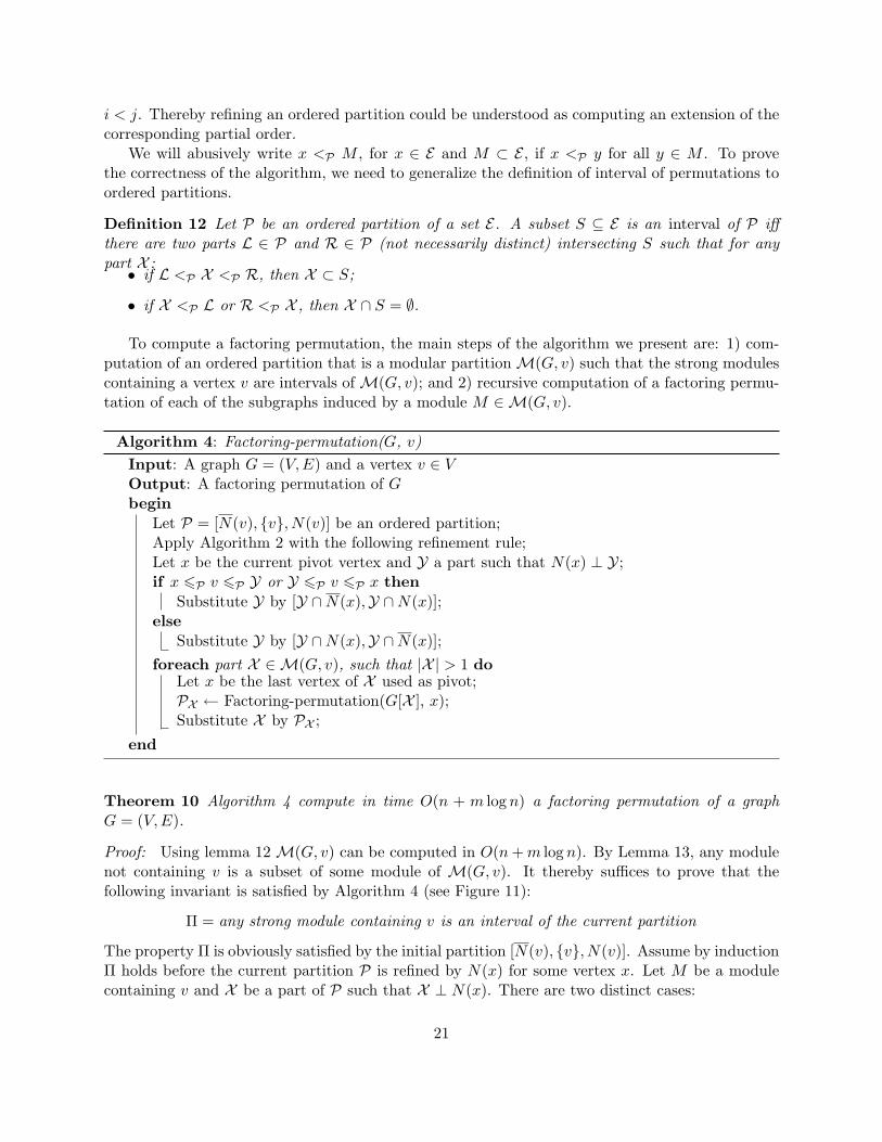
Figure 11: Layout of the modular decomposition tree MD(G) such that the neighbours of v areplaced on the right of v and the non-neighbours on the left. The right tree enlights the modulesof M(G, v) and the strong modules M1,M2,M3 and M4 containing v. Algorithm 4 first computesthe partition M(G, v) and then recursively solves the problem on each module of M(G, v)

• x /∈M : no vertex y of X ∩N(x) belongs to M , otherwise x would be a splitter for v and y;

• x ∈ M : if X ⊂ N(v), then any vertex y ∈ X ∩ N(x) belong to M , otherwise y would be asplitter for x and v. Similarly if X ⊂ N(v), then any vertex y ∈ X ∩N(x) belongs to M .

It follows that P ′ =Refine(P, N(x)) also satisfies the invariant Π. The complexity analysis is similarto the analysis of Algorithm 2. �

6.2 The case of cographs

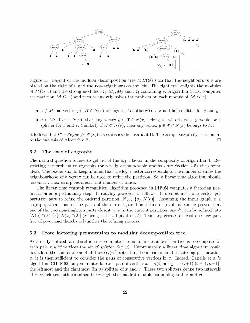
The natural question is how to get rid of the log n factor in the complexity of Algorithm 4. Re-stricting the problem to cographs (or totally decomposable graphs - see Section 2.5) gives someideas. The reader should keep in mind that the log n factor corresponds to the number of times theneighbourhood of a vertex can be used to refine the partition. So, a linear time algorithm shoulduse each vertex as a pivot a constant number of times.

The linear time cograph recognition algorithm proposed in [HP05] computes a factoring per-mutation as a preliminary step. It roughly proceeds as follows. It uses at most one vertex perpartition part to refine the ordered partition [N(v), {v}, N(v)]. Assuming the input graph is acograph, when none of the parts of the current partition is free of pivot, it can be proved thatone of the two non-singleton parts closest to v in the current partition, say X , can be refined into[N(x) ∩ X , {x}, N(x) ∩ X ] (x being the used pivot of X ). This step creates at least one new partfree of pivot and thereby relaunches the refining process.

6.3 From factoring permutation to modular decomposition tree

As already noticed, a natural idea to compute the modular decomposition tree is to compute foreach pair x, y of vertices the set of splitter S(x, y). Unfortunately a linear time algorithm couldnot afford the computation of all these O(n2) sets. But if one has in hand a factoring permutationσ, it is then sufficient to consider the pairs of consecutive vertices in σ. Indeed, Capelle et al.’salgorithm [CHdM02] only computes for each pair of vertices x = σ(i) and y = σ(i+1) (i ∈ [1, n−1])the leftmost and the rightmost (in σ) splitter of x and y. These two splitters define two intervalsof σ, which are both contained in m(x, y), the smallest module containing both x and y:

22

• the left fracture Fl(x, y) = [z, x] if z is the leftmost splitter of {x, y} in [σ(1), y] (if any);

• the right fracture Fd(x, y) = [y, z] if z is the rightmost splitter of {x, y} in [x, σ(n)] (if any).

(

1

2

3

4

5

6

7

8

9

10

11

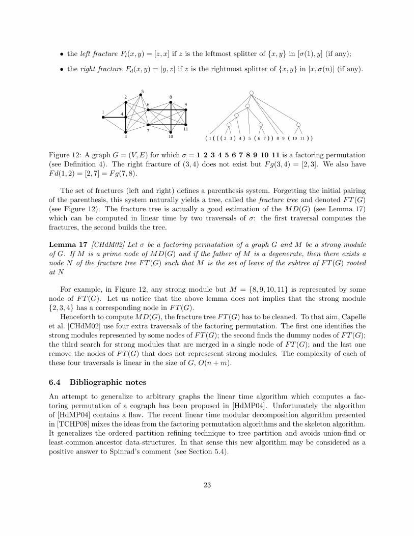
2 3 4 5 6 71 8 9 10 11 ))())())(((

Figure 12: A graph G = (V,E) for which σ = 1 2 3 4 5 6 7 8 9 10 11 is a factoring permutation(see Definition 4). The right fracture of (3, 4) does not exist but Fg(3, 4) = [2, 3]. We also haveFd(1, 2) = [2, 7] = Fg(7, 8).

The set of fractures (left and right) defines a parenthesis system. Forgetting the initial pairingof the parenthesis, this system naturally yields a tree, called the fracture tree and denoted FT (G)(see Figure 12). The fracture tree is actually a good estimation of the MD(G) (see Lemma 17)which can be computed in linear time by two traversals of σ: the first traversal computes thefractures, the second builds the tree.

Lemma 17 [CHdM02] Let σ be a factoring permutation of a graph G and M be a strong moduleof G. If M is a prime node of MD(G) and if the father of M is a degenerate, then there exists anode N of the fracture tree FT (G) such that M is the set of leave of the subtree of FT (G) rootedat N

For example, in Figure 12, any strong module but M = {8, 9, 10, 11} is represented by somenode of FT (G). Let us notice that the above lemma does not implies that the strong module{2, 3, 4} has a corresponding node in FT (G).

Henceforth to computeMD(G), the fracture tree FT (G) has to be cleaned. To that aim, Capelleet al. [CHdM02] use four extra traversals of the factoring permutation. The first one identifies thestrong modules represented by some nodes of FT (G); the second finds the dummy nodes of FT (G);the third search for strong modules that are merged in a single node of FT (G); and the last oneremove the nodes of FT (G) that does not represesent strong modules. The complexity of each ofthese four traversals is linear in the size of G, O(n+m).


An attempt to generalize to arbitrary graphs the linear time algorithm which computes a fac-toring permutation of a cograph has been proposed in [HdMP04]. Unfortunately the algorithmof [HdMP04] contains a flaw. The recent linear time modular decomposition algorithm presentedin [TCHP08] mixes the ideas from the factoring permutation algorithms and the skeleton algorithm.It generalizes the ordered partition refining technique to tree partition and avoids union-find orleast-common ancestor data-structures. In that sense this new algorithm may be considered as apositive answer to Spinrad’s comment (see Section 5.4).

23

7 Three novel applications of the modular decomposition

As mentioned in the introduction modular decomposition is used in a number of algorithmic graphtheory applications and more generally applies to various discrete structures (see [MR84]). Weconclude this survey with the presentation of three novel applications which are good witnesses ofthe use of modular decomposition. The first one is a pattern matching problem which is closelyrelated to the concept of factoring permutations. The second one provides an example of dynamicprogramming on the modular decomposition tree in the context of comparative genomic. Finally,we list a series of parameterized problems for which module based data-reduction rules leads topolynomial size kernels.

7.1 Pattern matching - common intervals of two permutations

Motivated by a series of genetic algorithms for sequencing problems, e.g. the TSP, Uno andYagiura [UY00] formalized the concept of common interval of two permutations. As we will seein the next subsection, in the context of comparative genonic, common intervals reveal conservedstructures in chromosomal material.

Definition 13 A set S of elements is a common interval of a set of permutations Σ if in eachpermutation σ ∈ Σ, the elements of S form an interval of σ (see Section 2.2 for the definition ofan interval).

It is fairly easy to observe that the family I of common intervals of two permutations is a weaklypartitive family (see Definition 1) and thus all the results from the theory presented in Section 2.1apply. In particular, the set of strong common intervals are organized into a tree, namely the stronginterval tree.

2

1110987641 2 3

16 7 5 10 11 9 8 4 3

5

Figure 13: The strong interval tree of two permutations. Remark {9, 10, 11} and {8, 9} are also acommon interval, but they are not strong as they overlap.

Despite of the existence of the (weakly) partitive set theory for more that thirty years, the nat-ural concept of interval substitution and decomposition appeared only very recently in the contextof the combinatorial study of permutations (see e.g. [AS02, AA05]). Atkinson and Stitt [AS02](re)discovered the concept of substitution under the name of wreath product. In 2005, Albert andAtkinson showed that, if the number of simple (i.e. prime) permutations in a pattern restrictedclass of permutations is finite, the class has an algebraic generating function and is defined by

24

a finite set of restrictions. More recently, Bouvel, Rossin and Viallette [BR06, BRV07] used thestrong interval tree to solve the longest common pattern problem between two permutations.

Uno and Yagiura [UY00] proposed the first linear time algorithm to enumerate the commonintervals of two permutations. More precisely, it runs in O(n+K) time, where K is the number ofthose common intervals (which is possibly quadratic). Alternative algorithms have been recentlyproposed [HMS09, BCdMR08]. We sketch Uno and Yagiura’s algorithm and discuss how it can begenralized to compute the modules of a graph when a factoring permutation is given.

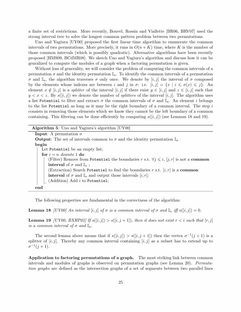
Without loss of generality, we will consider the problem of computing the common intervals of apermutation σ and the identity permutation In. To identify the common intervals of a permutationσ and In, the algorithm traverses σ only once. We denote by [i, j] the interval of σ composedby the elements whose indexes are between i and j in σ: i.e. [i, j] = {x | i 6 σ(x) 6 j}. Anelement x /∈ [i, j] is a splitter of the interval [i, j] if there exist y ∈ [i, j] and z ∈ [i, j] such thaty < x < z. By s([i, j]) we denote the number of splitters of the interval [i, j]. The algorithm usesa list Potentiel to filter and extract σ the common intervals of σ and In. An element i belongsto the list Potentiel as long as it may be the right boundary of a common interval. The step iconsists in removing those elements which we know they cannot be the left boundary of a commoncontaining. This filtering can be done efficiently by computing s([i, j]) (see Lemmas 18 and 19).

Algorithm 5: Uno and Yagiura’s algorithm [UY00]Input: A permutation σOutput: The set of intervals common to σ and the identity permutation In

beginLet Potentiel be an empty list;for i = n downto 1 do

(Filter) Remove from Potentiel the boundaries r s.t. ∀j 6 i, [j, r] is not a commoninterval of σ and In ;(Extraction) Search Potentiel to find the boundaries r s.t. [i, r] is a commoninterval of σ and In and output those intervals [i, r];(Addition) Add i to Potentiel;

end

The following properties are fundamental in the correctness of the algorithm:

Lemma 18 [UY00] An interval [i, j] of σ is a common interval of σ and In iff s([i, j]) = 0.

Lemma 19 [UY00, BXHP05] If s([i, j]) > s([i, j + 1]), then it does not exist r < i such that [r, j]is a common interval of σ and In.

The second lemma above means that if s([i, j]) > s([i, j + 1]) then the vertex σ−1(j + 1) is asplitter of [i, j]. Thereby any common interval containing [i, j] as a subset has to extend up toσ−1(j + 1).

Application to factoring permutations of a graph. The most striking link between commonintervals and modules of graphs is observed on permutation graphs (see Lemma 20). Permuta-tion graphs are defined as the intersection graphs of a set of segments between two parallel lines

25

(see [Gol80, BLS99] for example). It follows that the vertices of a permutation graph G = (V,E)can be numbered from 1 to n such that there exists a permutation σ of [1, n] such that vertexnumbered i is adjacent to vertex numbered j iff i < j and σ(j) < σ(i). The permutations σ and In

form the realizer of G. As first observed by de Montgolfier, any permutation belonging to a realizerof a permutation graph is a factorizing permutation of that graph. It follows from Lemma 1 that:

Lemma 20 [dM03] Let G = (V,E) be a permutation graph and (In, σ) be its realizer. A set ofvertices M is a strong module iff M is a strong common interval of In and σ.

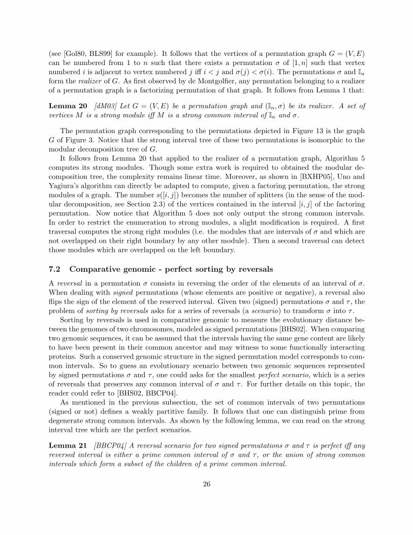
The permutation graph corresponding to the permutations depicted in Figure 13 is the graphG of Figure 3. Notice that the strong interval tree of these two permutations is isomorphic to themodular decomposition tree of G.

It follows from Lemma 20 that applied to the realizer of a permutation graph, Algorithm 5computes its strong modules. Though some extra work is required to obtained the modular de-composition tree, the complexity remains linear time. Moreover, as shown in [BXHP05], Uno andYagiura’s algorithm can directly be adapted to compute, given a factoring permutation, the strongmodules of a graph. The number s([i, j]) becomes the number of splitters (in the sense of the mod-ular decomposition, see Section 2.3) of the vertices contained in the interval [i, j] of the factoringpermutation. Now notice that Algorithm 5 does not only output the strong common intervals.In order to restrict the enumeration to strong modules, a slight modification is required. A firsttraversal computes the strong right modules (i.e. the modules that are intervals of σ and which arenot overlapped on their right boundary by any other module). Then a second traversal can detectthose modules which are overlapped on the left boundary.

7.2 Comparative genomic - perfect sorting by reversals

A reversal in a permutation σ consists in reversing the order of the elements of an interval of σ.When dealing with signed permutations (whose elements are positive or negative), a reversal alsoflips the sign of the element of the reserved interval. Given two (signed) permutations σ and τ , theproblem of sorting by reversals asks for a series of reversals (a scenario) to transform σ into τ .

Sorting by reversals is used in comparative genomic to measure the evolutionary distance be-tween the genomes of two chromosomes, modeled as signed permutations [BHS02]. When comparingtwo genomic sequences, it can be assumed that the intervals having the same gene content are likelyto have been present in their common ancestor and may witness to some functionally interactingproteins. Such a conserved genomic structure in the signed permutation model corresponds to com-mon intervals. So to guess an evolutionary scenario between two genomic sequences representedby signed permutations σ and τ , one could asks for the smallest perfect scenario, which is a seriesof reversals that preserves any common interval of σ and τ . For further details on this topic, thereader could refer to [BHS02, BBCP04].

As mentioned in the previous subsection, the set of common intervals of two permutations(signed or not) defines a weakly partitive family. It follows that one can distinguish prime fromdegenerate strong common intervals. As shown by the following lemma, we can read on the stronginterval tree which are the perfect scenarios.

Lemma 21 [BBCP04] A reversal scenario for two signed permutations σ and τ is perfect iff anyreversed interval is either a prime common interval of σ and τ , or the union of strong commonintervals which form a subset of the children of a prime common interval.

26

5 1110987641 2 3

16 7 5 10 11 9 8 4 32

1 67 5 9 8 4 23

1 2 3 8 9 5 64

11 10

10 11

1 2 3 4 5

7

7 6 891011

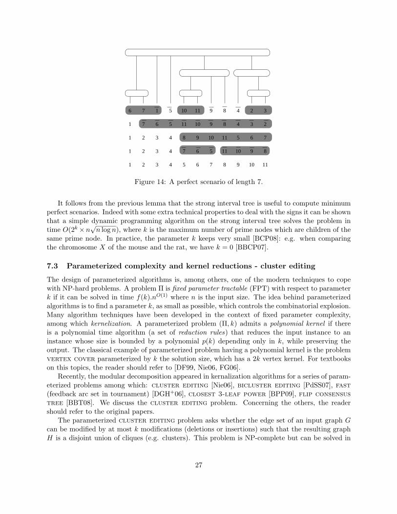
Figure 14: A perfect scenario of length 7.

It follows from the previous lemma that the strong interval tree is useful to compute minimumperfect scenarios. Indeed with some extra technical properties to deal with the signs it can be shownthat a simple dynamic programming algorithm on the strong interval tree solves the problem intime O(2k ×n

√n log n), where k is the maximum number of prime nodes which are children of the

same prime node. In practice, the parameter k keeps very small [BCP08]: e.g. when comparingthe chromosome X of the mouse and the rat, we have k = 0 [BBCP07].

7.3 Parameterized complexity and kernel reductions - cluster editing

The design of parameterized algorithms is, among others, one of the modern techniques to copewith NP-hard problems. A problem Π is fixed parameter tractable (FPT) with respect to parameterk if it can be solved in time f(k).nO(1) where n is the input size. The idea behind parameterizedalgorithms is to find a parameter k, as small as possible, which controls the combinatorial explosion.Many algorithm techniques have been developed in the context of fixed parameter complexity,among which kernelization. A parameterized problem (Π, k) admits a polynomial kernel if thereis a polynomial time algorithm (a set of reduction rules) that reduces the input instance to aninstance whose size is bounded by a polynomial p(k) depending only in k, while preserving theoutput. The classical example of parameterized problem having a polynomial kernel is the problemvertex cover parameterized by k the solution size, which has a 2k vertex kernel. For textbookson this topics, the reader should refer to [DF99, Nie06, FG06].

Recently, the modular decomposition appeared in kernalization algorithms for a series of param-eterized problems among which: cluster editing [Nie06], bicluster editing [PdSS07], fast(feedback arc set in tournament) [DGH+06], closest 3-leaf power [BPP09], flip consensustree [BBT08]. We discuss the cluster editing problem. Concerning the others, the readershould refer to the original papers.

The parameterized cluster editing problem asks whether the edge set of an input graph Gcan be modified by at most k modifications (deletions or insertions) such that the resulting graphH is a disjoint union of cliques (e.g. clusters). This problem is NP-complete but can be solved in

27

time O∗(3k) by a simple bounded search tree algorithm [Cai96], which iteratively branches on atmost k P3’s. Recent papers [Guo07, FLRS07] showed the existence of a linear kernel (best boundis 4k). The reduction rules used for these linear kernels are crown rules involving modules. For thesake of simplicity we only present the two basic reduction rules which leads to a quadratic vertexkernel.

Lemma 22 Let G = (V,E) be a graph. A quadratic vertex kernel for the cluster editingproblem is obtained by the following reduction rules:

1. Remove from G the connected components which are cliques.

2. If G contains a clique module C of size at least k + 1, then remove from |C| − k − 1 vertexfrom C.

It is clear that these rules can be applied in linear time using modular decomposition algorithms.The proof idea works as follows. The first rule is obviously safe. Concerning the second rule, simplyobserve that to disconnect a clique module of size k+1 from the rest of the graph, at least k+1 edgedeletions are required. Now assuming G is a positive instance, each cluster of the resulting graphH can be bipartitioned into the vertices non-incident to a modified edge and the other vertices (theaffected vertices). Finally k edge modifications can create at most 2k clusters and the total numberof affected vertices is bounded by 2k. This shows that the number of vertices in the reduced graphH is at most 2k2 + 4k.

The bicluster editing problem edits the edge set of a graph to obtain a disjoint union ofcomplete bipartite graphs. Instead of considering clique modules, we need to consider independentset modules [PdSS07]. The proof is then slightly more complicated and relies on a careful analysisof the modification of the modular decomposition under edge insertion or deletion. In the caseof fast, similar rules involving transitive modules also yields a quadratic kernel bound. Notethat for these two problems, linear kernels can be obtained with more sophisticated reductionrules [GHKZ08, BFG+09].

8 Conclusions and perspectives

An important remaining open problem is the proposal of a simple linear time certifying algorithmfor modular decomposition. In fact the algorithms described here produce a labelled tree that canbe checked in linear time if they are decomposition trees. But for certifying that some decompo-sition tree is the modular decomposition one must certify all node labels. The bottleneck is thecertification of prime nodes.

We have presented above the principles of a fully dynamic algorithm for modular decompositionof cographs, these can be also done for permutation graphs and interval graphs using their geometricrepresentation [CP06, Cre09]. Fully dynamic modular decomposition for the general case is still anopen problem.

For some applications one wants to extend the notion of module to some notion of approximativemodule, for which we want to extend the notion having the same behaviour outside of the module.Several attemps have already been considered [BXHLdM09]. The main difficulty is to find aninteresting extension of module polynomially tractable, since many of the natural extensions yieldto NP-complete problems [FP03].

28

References

[AA05] M. Albert and M. Atkinson. Simple permutations and pattern restricted permuta-tions. Discrete Mathematics, 300(1-3):1 – 15, 2005.

[AS02] M. Atkinson and T. Stitt. Restricted permutations and the wreath product. DiscreteMathematics, 259(1-3):19 – 36, 2002.

[BBCP04] A. Bergeron, S. Berard, C. Chauve, and C. Paul. Sorting by reversal is not alwaysdifficult. In Workshop on Algorithm for Bio-Informatics (WABI), Lecture Notes inComputer Science, 2004.

[BBCP07] S. Berard, A. Bergeron, C. Chauve, and C. Paul. Perfect sorting by reversals is notalways difficult. IEEE/ACM Trans. Comput. Biology Bioinform., 4(1):4–16, 2007.

[BBT08] S. Bocker, Q.B. Anh Bui, and A. Truß. An improved fixed-parameter algorithmfor minimum-flip consensus trees. In International Workshop on Parameterized andExact Computation (IWPEC), number 5018 in Lecture Notes in Computer Science,pages 43–54, 2008.

[BCdMR05] A. Bergeron, C. Chauve, F. de Montgolfier, and M. Raffinot. Computing commonintervals of k permutations, with applications to modular decomposition of graphs.In European Symposium on Algorithms (ESA), number 3669 in Lecture Notes inComputer Science, pages 779–790, 2005.

[BCdMR08] Anne Bergeron, Cedric Chauve, Fabien de Montgolfier, and Mathieu Raffinot. Com-puting common intervals of k permutations, with applications to modular decompo-sition of graphs. SIAM Journal on Discrete Mathematics, 22(3):1022–1039, 2008.

[BCHP03] A. Bretscher, D.G. Corneil, M. Habib, and C. Paul. A simple linear time LexBFScograph recognition algorithm. In 29th International Workshop on Graph-TheoreticConcepts in Computer Science (WG), volume 2880 of Lecture Notes in ComputerScience, pages 119–130, 2003.

[BCHP08] A. Bretscher, D. Corneil, M. Habib, and C. Paul. A simple linear time lexbfs cographrecognition algorithm. SIAM Journal on Discrete Mathematics, 22(4):1277–1296,2008.

[BCP08] S. Berard, C. Chauve, and C. Paul. A more efficient algorithm for perfect sortingby reversals. Information Processing Letters, 106:90–95, 2008.

[BFG+09] Stephane Bessy, Fedor V. Fomin, Serge Gaspers, Christophe Paul, Anthony Perez,Saket Saurabh, and Stephan Thomasse. Kernels for feedback arc set in tournaments.Technical Report CoRR abs/0907.2165, arxiv, 2009.

[BHS02] A. Bergeron, S. Herber, and J. Stoye. Common intervals and sorting by reversals: amariage of necessity. In European Conference on Computational Biology, Bioinfor-matics, pages 54–63, 2002.

29

https://www.researchgate.net/publication/220533232_Computing_Common_Intervals_of_K_Permutations_with_Applications_to_Modular_Decomposition_of_Graphs?el=1_x_8&enrichId=rgreq-396046a6dea7d3687a99176a657ce484-XXX&enrichSource=Y292ZXJQYWdlOzIyMjQxODU3MTtBUzoxMDM2MTg0NzI1NzkwNzVAMTQwMTcxNTk3NzE5Mw==








https://www.researchgate.net/publication/222677629_Kernels_for_Feedback_Arc_Set_In_Tournaments?el=1_x_8&enrichId=rgreq-396046a6dea7d3687a99176a657ce484-XXX&enrichSource=Y292ZXJQYWdlOzIyMjQxODU3MTtBUzoxMDM2MTg0NzI1NzkwNzVAMTQwMTcxNTk3NzE5Mw==



[Bla78] A. Blass. Graphs with unique maximal clumpings. Journal of Graph Theory, 2:19–24,1978.

[BLS99] A. Brandstadt, VB. Le, and J. Spinrad. Graph classes: a survey. SIAM Monographson Discrete Mathematics and Applications. Society for Industrial and Applied Math-ematics, 1999.

[BPP09] S. Bessy, C. Paul, and A. Perez. Polynomial kernels for 3-leaf power graph modifica-tion problems. In International Workshop on Combinatorial Algorithm (IWOCA),Lecture Notes in Computer Science, 2009.

[BR06] M. Bouvel and D. Rossin. The longest common pattern problem for two permuta-tions. Pure Mathematics and Applications, 17(1-2):55–69, 2006.

[BRV07] M. Bouvel, D. Rossin, and S. Vialette. Longest common separable pattern amongpermutations. In Annual Symposium on Combinatorial Pattern Matching (CPM),number 4580 in Lecture Notes in Computer Science, pages 316–327, 2007.

[BX08] B.M. Bui-Xuan. Tree-representation of set families in graph decompositions andefficient algorithms. PhD thesis, Univ. de Montpellier II, 2008.

[BXH08] B.-M. Bui-Xuan and M. Habib. A representation theorem for union-difference fam-ilies and application. In Latin American Symposium on Theoretical Informatics(LATIN), volume 4957 of Lecture Notes in Computer Science, pages 492–503, 2008.

[BXHLdM09] B-M. Bui-Xuan, M. Habib, V. Limouzy, and F. de Montgolfier. Algorithmic as-pects of a general modular decomposition theory. Discrete Applied Mathematics,157(9):1993–2009, 2009.

[BXHP05] B.-M. Bui-Xuan, M. Habib, and C. Paul. Revisiting uno and yagiura’s algorithm.In 16th International Symposium on Algorithms and Computation (ISAAC), volume3827 of Lecture Notes in Computer Science, pages 146–155, 2005.

[Cai96] L. Cai. Fixed-parameter tractability of graph modification problems for hereditaryproperties. Information Processing Letters, 58(4):171–176, 1996.

[Cap97] C. Capelle. Decomposition de graphes et permutations factorisantes. PhD thesis,Univ. de Montpellier II, 1997.

[CE80] W.H. Cunnigham and J. Edmonds. A combinatorial decomposition theory. CanadianJournal of Mathematics, 32(3):734–765, 1980.

[CER93] B. Courcelle, J. Engelfriet, and G. Rozenberg. Handle rewriting graph grammars.Journal of Computer and System Science, 46:218–270, 1993.

[CH94] A. Cournier and M. Habib. A new linear algorithm of modular decomposition. InTrees in algebra and programming (CAAP), volume 787 of Lecture Notes in ComputerScience, pages 68–84, 1994.

30

https://www.researchgate.net/publication/229712544_Graph_with_unique_maximal_clumping?el=1_x_8&enrichId=rgreq-396046a6dea7d3687a99176a657ce484-XXX&enrichSource=Y292ZXJQYWdlOzIyMjQxODU3MTtBUzoxMDM2MTg0NzI1NzkwNzVAMTQwMTcxNTk3NzE5Mw==

https://www.researchgate.net/publication/229712544_Graph_with_unique_maximal_clumping?el=1_x_8&enrichId=rgreq-396046a6dea7d3687a99176a657ce484-XXX&enrichSource=Y292ZXJQYWdlOzIyMjQxODU3MTtBUzoxMDM2MTg0NzI1NzkwNzVAMTQwMTcxNTk3NzE5Mw==

[CH97] C. Capelle and M. Habib. Graph decompositions and factorizing permutations. InFifth Israel Symposium on Theory of Computing and Systems - ISTCS, IEEE Conf.PR08037, Ramat-Gan, Israel, pages 132–143, 1997.

[CHdM02] C. Capelle, M. Habib, and F. de Montgolfier. Graph decompositions and factorizingpermutations. Discrete Mathematics and Theoretical Computer Science, 5:55–70,2002.

[CHM81] M. Chein, M. Habib, and M.-C. Maurer. Partitive hypergraphs. Discrete Mathemat-ics, 37:35–50, 1981.

[CI98] A. Cournier and P. Ille. Minimal indecomposable graphs. Discrete Mathematics,183:61–80, 1998.

[CJS72] D.D. Cowan, L.O. James, and R.G. Stanton. Graph decomposition for undirectedgraphs. In 3rd S-E Conference on Combinatorics, Graph Theory and Computing,Utilitas Math, pages 281–290, 1972.

[CLR90] T.H. Cormen, C.E. Leiserson, and R.L. Rivest. Algorithms. MIT Press, 1990.

[CLSB81] D.G. Corneil, H. Lerchs, and L.K. Stewart-Burlingham. Complement reduciblegraphs. Discrete Applied Mathematics, 3(1):163–174, 1981.

[Cor04a] D. G. Corneil. A simple 3-sweep LBFS algorithm for the recognition of unit intervalgraphs. Discrete Applied Mathematics, 138(3):371–379, 2004.

[Cor04b] D.G. Corneil. Lexicographic Breadth First Search - a survey. In 30th InternationalWorkshop on Graph-Theoretic Concepts in Computer Science (WG), volume 3353of Lecture Notes in Computer Science, pages 1–19, 2004.

[CP06] C. Crespelle and C. Paul. Fully-dynamic recognition algorithm and certificate fordirected cographs. Discrete Applied Mathematics, 154(12):1722–1741, 2006.

[CPS85] D.G. Corneil, Y. Perl, and L.K. Stewart. A linear time recognition algorithm forcographs. SIAM Journal on Computing, 14(4):926–934, 1985.

[Cre09] C. Crespelle. Fully dynamic representation of interval graphs. In Internation Work-shop on Graph Theoretical Concepts in Computer Science (WG), 2009.

[Cun82] W.H. Cunningham. Decomposition of directed graphs. SIAM Journal on Algebraicand Discrete Methods, 3:214–228, 1982.

[Dah95] E. Dahlhaus. Efficient parallel algorithms for cographs and distance hereditarygraphs. Discrete Applied Mathematics, 57:29–54, 1995.

[DF99] R.G. Downey and M.R. Fellows. Parameterized complexity. Springer, 1999.

[DGH+06] M. Dom, J. Guo, F. Huffner, R. Niedermeier, and A. Truss. Fixed-parametertractability results for feedback set problems in tournaments. In Italian Conferenceon Algorithms and Complexity (CIAC), volume 3998 of Lecture Notes in ComputerScience, pages 320–331, 2006.

31

https://www.researchgate.net/publication/225736596_Fixed-Parameter_Tractability_Results_for_Feedback_Set_Problems_in_Tournaments?el=1_x_8&enrichId=rgreq-396046a6dea7d3687a99176a657ce484-XXX&enrichSource=Y292ZXJQYWdlOzIyMjQxODU3MTtBUzoxMDM2MTg0NzI1NzkwNzVAMTQwMTcxNTk3NzE5Mw==







https://www.researchgate.net/publication/2602962_Graph_Decompositions_and_Factorizing_Permutations?el=1_x_8&enrichId=rgreq-396046a6dea7d3687a99176a657ce484-XXX&enrichSource=Y292ZXJQYWdlOzIyMjQxODU3MTtBUzoxMDM2MTg0NzI1NzkwNzVAMTQwMTcxNTk3NzE5Mw==



[DGM01] E. Dahlhaus, J. Gustedt, and R.M. McConnell. Efficient and practical algorithm forsequential modular decomposition algorithm. Journal of Algorithms, 41(2):360–387,2001.

[dM03] F. de Mongolfier. Decomposition modulaire des graphes - Theorie, extensions etalgorithmes. PhD thesis, Univ. de Montpellier II, 2003.

[EG97] J. Edmonds and R. Giles. A min-max relation for submodular functions on graphs.Annals of Discrete Mathematics, 1:185–204, 1997.

[EGMS94] A. Ehrenfeucht, H.N. Gabow, R.M. McConnell, and S.L. Sullivan. An O(n2) divide-and-conquer algorithm for the prime tree decomposition of two-structures and mod-ular decomposition of graphs. Journal of Algorithms, 16:283–294, 1994.

[EHR99] A. Ehrenfeucht, T. Harju, and G. Rozenberg. The theory of 2-structures. WorldScientific, 1999.

[ER90] A. Ehrenfeucht and G. Rozenberg. Primitivity is hereditary for 2-structures. Theo-retical Computer Science, 70(3):343 – 358, 1990.

[FG06] J. Flum and M. Grohe. Parameterized complexity theorey. Texts in TheoreticalComputer Science. Springer, 2006.

[FHdMV04] J.-L. Fouquet, M. Habib, F. de Montgolfier, and J.-M. Vanherpe. Bimodular de-composition of bipartite graphs. In International Workshop on Graph TheoreticalConcepts in Computer Science (WG), volume 3353 of Lecture Notes in ComputerScience, pages 117–128, 2004.

[FLRS07] M.R. Fellows, M. Langston, F. Rosamond, and P. Shaw. Efficient parameterizedpreprocessing for cluster editing. In International Symposium on Fundamentals ofComputation Theory (FCT), number 4639 in Lecture Notes in Computer Science,pages 312–321, 2007.

[FP03] Jirı Fiala and Daniel Paulusma. The computational complexity of the role assignmentproblem. In International Colloquium on Automata, Languages and Programming(ICALP), volume 2719 of Lecture Notes in Computer Science, pages 817–828, 2003.

[Gal67] T. Gallai. Transitiv orientierbare graphen. Acta Mathematica Acad. Sci. Hungar.,18:25–66, 1967.

[GHKZ08] J. Guo, F. Huffner, C. Komusiewicz, and Y. Zhang. Improved algorithms for biclusterediting. In Annual Conference on Theory and Applications of Models of Computation(TAMC), volume 4978 of Lecture Notes in Computer Science, pages 445–456, 2008.

[Gol80] M.C. Golumbic. Algorithmic graph theory and perfect graphs. Academic Press, 1980.

[GP07] E. Gioan and C. Paul. Dynamic distance hereditary graphs using split decomposition.In International Symposium on Algorithms and Computation (ISAAC), volume 4884of Lecture Notes in Computer Science, 2007.

32

https://www.researchgate.net/publication/220898875_The_Computational_Complexity_of_the_Role_Assignment_Problem?el=1_x_8&enrichId=rgreq-396046a6dea7d3687a99176a657ce484-XXX&enrichSource=Y292ZXJQYWdlOzIyMjQxODU3MTtBUzoxMDM2MTg0NzI1NzkwNzVAMTQwMTcxNTk3NzE5Mw==






[GPTC09a] E. Gioan, C. Paul, M. Tedder, and D. Corneil. Practical split-decomposition viagraph-labelled trees. Submitted, 2009.

[GPTC09b] E. Gioan, C. Paul, M. Tedder, and D. Corneil. Quasi-linear circle graph recognition.Submitted, 2009.

[Guo07] J. Guo. A more effective linear kernelization for cluster editing. In InternationalSymposiumCombinatorics, Algorithms, Probabilistic and Experimental Methodolo-gies (ESCAPE), volume 4614 of Lecture Notes in Computer Science, pages 36–47,2007.

[HdMP04] M. Habib, F. de Montgolfier, and C. Paul. A simple linear-time modular decom-position algorithm. In 9th Scandinavian Workshop on Algorithm Theory (SWAT),volume 3111 of Lecture Notes in Computer Science, pages 187–198, 2004.

[HHS95] M. Habib, M. Huchard, and J.S. Spinrad. A linear algorithm to decompose inheri-tance graphs into modules. Algorithmica, 13:573–591, 1995.

[HM79] M. Habib and M.-C. Maurer. On the x-join decomposition of undirected graphs.Discrete Applied Mathematics, 1:201–207, 1979.

[HM91] W.-L. Hsu and T.-H. Ma. Substitution decomposition on chordal graphs and ap-plications. In 2nd International Symposium on Algorithms (ISA), volume 557 ofLecture Notes in Computer Science, pages 52–60, 1991.

[HMPV00] M. Habib, R.M. McConnell, C. Paul, and L. Viennot. Lex-bfs and partition re-finement, with applications to transitive orientation, interval graph recognition andconsecutive ones testing. Theoretical Computer Science, 234:59–84, 2000.

[HMS09] S. Herber, R. Mayr, and J. Stoye. Common intervals of multiple permutations.Algorithmica, 2009.

[Hop71] J. Hopcroft. An n log n algorithm for minimizing states in a finite automaton. Theoryof machines and computations, pages 189–196, 1971.

[HP05] M. Habib and C. Paul. A simple linear time algorithm for cograph recognition.Discrete Applied Mathematics, 145(2):183–187, 2005.

[HPV98] M. Habib, C. Paul, and L. Viennot. A synthesis on partition refinement: a usefulroutine for strings, graphs, boolean matrices and automata. In 15th Symposium onTheoretical Aspect of Computer Science (STACS), volume 1373 of Lecture Notes inComputer Science, pages 25–38, 1998.

[HPV99] M. Habib, C. Paul, and L. Viennot. Partition refinement : an interesting algorithmictool kit. International Journal of Foundation of Computer Science, 10(2):147–170,1999.

[HSS01] P. Hell, R. Shamir, and R. Sharan. A fully dynamic algorithm for recongizingand representing propoer interval graphs. SIAM Journal on Discrete Mathemat-ics, 31(1):289–305, 2001.

33

https://www.researchgate.net/publication/245065602_A_Simple_Linear-Time_Modular_Decomposition_Algorithm?el=1_x_8&enrichId=rgreq-396046a6dea7d3687a99176a657ce484-XXX&enrichSource=Y292ZXJQYWdlOzIyMjQxODU3MTtBUzoxMDM2MTg0NzI1NzkwNzVAMTQwMTcxNTk3NzE5Mw==




[Hsu92] W.-L. Hsu. A simple test for interval graphs. In 3rd International Symposium onAlgorithms and Computation (ISAAC), volume 557 of Lecture Notes in ComputerScience, pages 459–468, 1992.

[Iba09] L. Ibarra. A fully dynamic graph algorithm for recognizing interval graphs. Algo-rithmica, 2009.

[JO92a] B. Jamison and S. Olariu. Recognizing p4-sparse graphs in linear time. SIAM Journalon Discrete Mathematics, 21:381–406, 1992.

[JO92b] B. Jamison and S. Olariu. A tree representation of p4-sparse graphs. Discrete AppliedMathematics, 35:115–129, 1992.

[JO95] B. Jamison and S. Olariu. P-components and the homogeneous decomposition ofgraphs. SIAM Journal on Discrete Mathematics, 8(3):448–463, 1995.

[Lov72] L. Lovasz. A characterization of perfect graphs. Journal of Combinatorial TheorySeries B, 13:95–98, 1972.

[Moh85a] R.H. Mohring. Algorithmic aspect of comparability graphs and interval graphs.Graphs and orders, pages 42–101, 1985.

[Moh85b] R.H. Mohring. Algorithmic aspect of the substitution decomposition in optimizationover relations, set systems and boolean functions. Annals of Operations Research,4:195–225, 1985.

[MR84] R.H. Mohring and F.J. Radermacher. Substitution decomposition for discrete struc-tures and connections with combinatorial optimization. Annals of Discrete Mathe-matics, 19:257–356, 1984.

[MS89] J.H. Muller and J.P. Spinrad. Incremental modular decomposition. Journal of theACM, 36(1):1–19, 1989.

[MS94] R.M. McConnell and J.P. Spinrad. Linear-time modular decomposition and efficienttransitive orientation of comparability graphs. In 5th Annual ACM-SIAM Sympo-sium on Discrete Algorithms (SODA), pages 536–545, 1994.

[MS99] R.M. McConnell and J.P. Spinrad. Modular decomposition and transitive orienta-tion. Discrete Mathematics, 201:189–241, 1999.

[MS00] R.M. McConnell and J.P. Spinrad. Ordered vertex partitioning. Discrete Mathemat-ics and Theoretical Computer Science, 4:45–60, 2000.

[Nie06] R. Niedermeier. Invitation to fixed parameter algorithms, volume 31 of Oxford Lec-tures Series in Mathematics and its Applications. Oxford University Press, 2006.

[PdSS07] F. Protti, M. Dantas da Silva, and J.L. Szwarcfiter. Applying modular decompositionto parameterized cluster editing problems. Theory of Computing Systems, 2007.

[PT87] R. Paigue and R.E. Tarjan. Three partition refinement algorithms. SIAM Journalon Computing, 16(6):973–989, 1987.

34

https://www.researchgate.net/publication/220617997_Recognizing_P_4_-Sparse_Graphs_in_Linear_Time?el=1_x_8&enrichId=rgreq-396046a6dea7d3687a99176a657ce484-XXX&enrichSource=Y292ZXJQYWdlOzIyMjQxODU3MTtBUzoxMDM2MTg0NzI1NzkwNzVAMTQwMTcxNTk3NzE5Mw==

https://www.researchgate.net/publication/220617997_Recognizing_P_4_-Sparse_Graphs_in_Linear_Time?el=1_x_8&enrichId=rgreq-396046a6dea7d3687a99176a657ce484-XXX&enrichSource=Y292ZXJQYWdlOzIyMjQxODU3MTtBUzoxMDM2MTg0NzI1NzkwNzVAMTQwMTcxNTk3NzE5Mw==

https://www.researchgate.net/publication/220752533_A_Simple_Test_for_Interval_Graphs?el=1_x_8&enrichId=rgreq-396046a6dea7d3687a99176a657ce484-XXX&enrichSource=Y292ZXJQYWdlOzIyMjQxODU3MTtBUzoxMDM2MTg0NzI1NzkwNzVAMTQwMTcxNTk3NzE5Mw==



https://www.researchgate.net/publication/222615393_A_tree_representation_for_P4-sparse_graphs?el=1_x_8&enrichId=rgreq-396046a6dea7d3687a99176a657ce484-XXX&enrichSource=Y292ZXJQYWdlOzIyMjQxODU3MTtBUzoxMDM2MTg0NzI1NzkwNzVAMTQwMTcxNTk3NzE5Mw==

https://www.researchgate.net/publication/222615393_A_tree_representation_for_P4-sparse_graphs?el=1_x_8&enrichId=rgreq-396046a6dea7d3687a99176a657ce484-XXX&enrichSource=Y292ZXJQYWdlOzIyMjQxODU3MTtBUzoxMDM2MTg0NzI1NzkwNzVAMTQwMTcxNTk3NzE5Mw==

[RST08] I. Rapaport, K. Suchan, and I. Todinca. Minimal proper interval completions. In-formation Processing Letters, 106(5):195–202, 2008.

[RTL76] D.J. Rose, R.E. Tarjan, and G.S. Lueker. Algorithmic aspects of vertex eliminationon graphs. SIAM Journal on Computing, 5(2):266–283, 1976.

[Spi03] J.P. Spinrad. Efficient graph representation, volume 19 of Fields Institute Mono-graphs. American Mathematical Society, 2003.

[SS04] R. Shamir and R. Sharan. A fully dynamic algorithm for modular decompositionand recognition of cographs. Discrete Applied Mathematics, 136(2-3):329–340, 2004.

[ST93] J. Schmerl and W. Trotter. Critically indecomposable partially ordered sets, graphs,tournaments and other binary relational structures. Discrete Mathematics, 113(1-3):191 – 205, 1993.

[Sum73] D.P. Sumner. Graphs indecomposable with respect to the x-join. Discrete Mathe-matics, 6:281–298, 1973.

[TCHP08] M. Tedder, D. Corneil, M. Habib, and C. Paul. Simpler linear-time modular de-composition via recursive factorizing permutations. In International Colloquium onAutomata, Languages and Programming (ICALP), volume 5125 (1) of Lecture Notesin Computer Science, pages 634–645, 2008.

[UY00] T. Uno and M. Yagiura. Fast algorithms to enumerate all common intervals of twopermutations. Algorithmica, 26(2):290–309, 2000.

35

https://www.researchgate.net/publication/222603788_Minimal_Proper_Interval_Completions?el=1_x_8&enrichId=rgreq-396046a6dea7d3687a99176a657ce484-XXX&enrichSource=Y292ZXJQYWdlOzIyMjQxODU3MTtBUzoxMDM2MTg0NzI1NzkwNzVAMTQwMTcxNTk3NzE5Mw==

https://www.researchgate.net/publication/222603788_Minimal_Proper_Interval_Completions?el=1_x_8&enrichId=rgreq-396046a6dea7d3687a99176a657ce484-XXX&enrichSource=Y292ZXJQYWdlOzIyMjQxODU3MTtBUzoxMDM2MTg0NzI1NzkwNzVAMTQwMTcxNTk3NzE5Mw==

A survey on algorithmic aspects of modular decomposition

Documents