A Survey of Trefftz Methods for the Helmholtz Equation R. Hiptmair and A. Moiola and I. Perugia Research Report No. 2015-20 June 2015 Seminar für Angewandte Mathematik Eidgenössische Technische Hochschule CH-8092 Zürich Switzerland ____________________________________________________________________________________________________ Funding SNF: PDFMP2-124883/1 (second author 09/09-08/12) To appear in Springer Lecture Notes on Computational Science and Engineering.

Welcome message from author
This document is posted to help you gain knowledge. Please leave a comment to let me know what you think about it! Share it to your friends and learn new things together.
Transcript

A Survey of Trefftz Methods for the
Helmholtz Equation
R. Hiptmair and A. Moiola and I. Perugia
Research Report No. 2015-20June 2015
Seminar für Angewandte MathematikEidgenössische Technische Hochschule
CH-8092 ZürichSwitzerland
____________________________________________________________________________________________________
Funding SNF: PDFMP2-124883/1 (second author 09/09-08/12)
To appear in Springer Lecture Notes on Computational Science and Engineering.

A Survey of Trefftz Methods for the HelmholtzEquation
Ralf Hiptmair, Andrea Moiola and Ilaria Perugia
Abstract Trefftz methods are finite element-type schemes whose test and trial func-
tions are (locally) solutions of the targeted differential equation. They are particu-
larly popular for time-harmonic wave problems, as their trial spaces contain oscillat-
ing basis functions and may achieve better approximation properties than classical
piecewise-polynomial spaces.
We review the construction and properties of several Trefftz variational formula-
tions developed for the Helmholtz equation, including least squares, discontinuous
Galerkin, ultra weak variational formulation, variational theory of complex rays and
wave based methods. The most common discrete Trefftz spaces used for this equa-
tion employ generalised harmonic polynomials (circular and spherical waves), plane
and evanescent waves, fundamental solutions and multipoles as basis functions; we
describe theoretical and computational aspects of these spaces, focusing in particu-
lar on their approximation properties.
One of the most promising, but not yet well developed, features of Trefftz meth-
ods is the use of adaptivity in the choice of the propagation directions for the basis
functions. The main difficulties encountered in the implementation are the assem-
bly and the ill-conditioning of linear systems, we briefly survey some strategies that
have been proposed to cope with these problems.
Ralf Hiptmair
Seminar for Applied Mathematics, ETH Zurich, 8092 Zurich, Switzerland, e-mail: hipt-
Andrea Moiola
Department of Mathematics and Statistics, University of Reading, Whiteknights PO Box 220, RG6
6AX, UK, e-mail: [email protected]
Ilaria Perugia
Faculty of Mathematics, University of Vienna, 1090 Vienna, Austria, and Department of Mathe-
matics, University of Pavia, 27100 Pavia, Italy, e-mail: [email protected]
1

2 Ralf Hiptmair, Andrea Moiola and Ilaria Perugia
1 Introduction
Given a linear PDE, a Trefftz method is a volume-oriented discretisation scheme, for
which all trial and test functions, when restricted to any element of a given mesh, are
solutions of the PDE under consideration. The name comes from the work [112] of
E. Trefftz, dating back to 1926, where this idea was applied to the Laplace equation.
Since then, several versions of Trefftz methods have been proposed and applied to a
range of PDEs by different groups of mathematicians, engineers and computational
scientists, often unaware of each other. Typical PDEs addressed are linear, with
piecewise-constant coefficients and homogeneous, i.e. with vanishing volume source
term.
Trefftz methods are related to both finite element (FEM) and boundary element
methods (BEM). With the former they have in common that they provide a dis-
cretisation in the volume. With the latter they share some characteristics such as the
need of integration on lower-dimensional manifolds only. Compared to conventional
FEMs, Trefftz methods have attracted attention mainly for two reasons: (i) they may
need much fewer degrees of freedom than standard schemes to achieve the same ac-
curacy, and (ii) they incorporate some properties of the problem’s solution (such as
oscillatory character, wavelength, maximum principle, boundary layers) in the trial
spaces, and thus also in the discrete solution. In addition, compared to BEMs, an
advantage of Trefftz schemes is that they do not require the evaluation of singular
integrals.
Comparing with finite and boundary elements, in 1997 Zienkiewicz [121] stated:
“. . . it seems without doubt that in the future Trefftz type elements will frequently
be encountered in general finite element codes.. . . It is the author’s belief that the
simple Trefftz approach will in the future displace much of the boundary type anal-
ysis with singular kernels.” While this prediction has not yet come true, in the last
years more and more work has been devoted to the formulation, the analysis and the
validation of these methods and substantial progress has been accomplished.
In this chapter we survey Trefftz finite element methods for the homogeneous
Helmholtz equation (−∆u− k2u = 0), which models acoustic wave propagation in
time-harmonic regime. For medium and high frequencies, i.e. for values of kL in a
range of 102 to 104, where k > 0 is the wavenumber, and L a characteristic length of
the region of interest, the numerical solution of the Helmholtz equation in 2D and
3D is particularly challenging. A main reason is that Helmholtz solutions oscillate
with a wavelength proportional to the inverse of k. Hence, piecewise polynomials do
not provide efficient approximation. Trefftz schemes are thus particularly relevant
as they can improve on the point where (polynomial) FEMs fail: the approximation
properties of the basis functions. Moreover, some Trefftz methods can remedy other
shortcomings that often haunt discretisations of time-harmonic problems, such as
the lack of coercivity and the presence of minimal resolution conditions to guarantee
unique solvability. Theorem 2 in this chapter is an example. Earlier overviews of
Trefftz schemes for the Helmholtz equation, together with numerous references,
can be found in [98], [85, Ch. 1] and [76, Ch. 3]. Surveys of Trefftz schemes for
other equations are in [67, 75, 99, 121].

A Survey of Trefftz Methods for the Helmholtz Equation 3
For most of the Trefftz spaces used, continuity across interfaces separating mesh
elements cannot be enforced strongly, as Trefftz functions are not as “flexible” as
piecewise polynomials. As a consequence, the standard Helmholtz variational for-
mulation posed in subspaces of the Sobolev space H1 is not applicable and discreti-
sations must be used that can accommodate discontinuous trial functions. A wide
array of different variational formulations has been proposed and in §2 we attempt
a classification and a comparison of the best known. We identify three main classes
of formulations: (i) least squares (LS, §2.1), where squares of suitable norms of
residuals are minimised; (ii) discontinuous Galerkin (DG, §2.2), whose formula-
tions arise from local integration by parts and which may or may not use Lagrange
multipliers on mesh interfaces; (iii) weighted residual (§2.3), which are defined by
testing residuals against suitable traces of test functions. The methods discussed
include: the Trefftz-discontinuous Galerkin (TDG), the ultra weak variational for-
mulation (UWVF), the discontinuous enrichment method (DEM), the variational
theory of complex rays (VTCR) and the wave based method (WBM). Moreover, in
the spirit of the symposium that led up to the present volume, to “build bridges” with
a wider portion of the literature and of the computational PDE community, in §2.4
we describe some older Trefftz schemes defined on a single element and in §2.5
we consider some methods that are not Trefftz but use oscillating basis functions
that are “approximately Trefftz”, such as the partition of unity method (PUM). To
easily compare them, we write all formulations for the same Robin–Dirichlet model
boundary value problem (see §1.1).
In §2 we completely gloss over the choice of basis functions and discrete spaces
employed, whose description is postponed to §3. This is because, apart from few ex-
ceptions such as unbounded elements, any Trefftz discrete space can be employed in
any Trefftz variational formulation. We believe that separating the discussion of the
two main components in the definition of a Trefftz method, i.e. variational formu-
lations and discrete spaces, will make the presentation clearer. The most common
basis functions for Trefftz methods are plane waves (x 7→ eikd·x for a fixed unit vector
d) and generalised harmonic polynomials (i.e. circular/spherical waves, products of
circular/spherical harmonics and Bessel functions), for which quite a complete ap-
proximation theory exists, see §3.1–3.2. Other basis functions include fundamental
solutions, multipoles, evanescent waves and corner waves. We note that, since the
Helmholtz operator is the sum of a second- and a zero-order term, no non-vanishing
piecewise-polynomial Trefftz function is possible.
In this chapter we state a few theorems, none of them is entirely new. Lemma 1
exemplifies the technique of [89] to control the L2 norm of Trefftz functions with
mesh-dependent norms containing interface jumps. If a Trefftz method is well-posed
in a suitable skeleton norm, this allows to control the error in the volume; we do this
for the LS method in Theorem 1 and for the TDG method (well-posed by Theo-
rem 2) in Corollary 1. This can be combined with the approximation results for
circular/spherical and plane waves in §3.1–§3.2. In brief: we provide the tools to
derive stability and orders of L2-convergence in the volume for all Trefftz methods
that are well-posed in suitable skeleton norms.
4 Ralf Hiptmair, Andrea Moiola and Ilaria Perugia
Trefftz methods suffer from two main problems: ill-conditioning due to the poor
linear independence of the basis functions, and the need for numerical quadrature
for oscillating integrands. On the other hand, since the PDE is solved exactly in each
element, only low-dimensional integrals on the mesh skeleton need to be evaluated,
leading to massively reduced computational cost for the assembly of the linear sys-
tems. Moreover, if plane wave bases are used, on any polygonal/polyhedral mesh
the integrals can be computed analytically in a cheap way. In §4 we briefly review
strategies developed to deal with the computation of matrix entries and to cope with
ill-conditioning.
Some Trefftz methods also provide an attractive framework for implementing
non-standard adaptive policies, like directional adaptivity following dominant wave
directions. This is made possible, because plane wave-type Trefftz functions natu-
rally encode a direction of propagation. More details are given in §4.2.
As mentioned, in this chapter we only discuss the Helmholtz equation, i.e. acous-
tic problems, and constant material parameters. The discrete Trefftz spaces used
for the Helmholtz equation with variable coefficients are briefly addressed in §3.4.
Other time-harmonic wave problems that have been tackled with Trefftz methods in-
clude electromagnetism (Maxwell equations) [18,85], linearised Euler equation and
general hyperbolic systems [37], linear elasticity (Navier equation) [76], (fourth or-
der) Kirchhoff–Love plates [27,70,76,100], Koiter’s linear shell theory [100], poro-
elasticity [27, §5.4], coupled vibro-acoustic problems [27]. A list of applications
and references can be found in [24, §5.1] (with a focus in vibrational mechanics)
and in [76, 85]. A related application is tackled by the method of particular solu-
tions (MPS) of [16, 36], which uses Helmholtz solutions to approximate Laplace
eigenvalue problems; in this setting the wavenumber is part of the unknowns. For
recent work on space–time Trefftz methods for wave propagation in time-domain
see [69] and references therein.
Several comparisons of the numerical performances of different Trefftz schemes
for simple model problems have been published, e.g. [7] (PUM, DEM, gener-
alised FEM), [40] (LS, UWVF), [60] (PUM, UWVF), [39] (DG, UWVF, LS), [115]
(DEM, UWVF, PUM), [59] (LS, UWVF, VTCR), where we have included the PUM
even if strictly speaking it is not a Trefftz method. However, from these results it is
difficult to conclude that any formulation is clearly preferable from a computational
point of view. A general conclusion might be that, in order to achieve the best ac-
curacy and conditioning, the choice of the approximation space matters more than
that of the variational formulation. We reiterate that these two choices are mutu-
ally independent: any Trefftz discrete space might be used in any Trefftz variational
formulation. We make some further concluding remarks in §5.
1.1 Model boundary value problem
We rely on a simple model boundary value problem (BVP) for the Helmholtz equa-
tion that will be used to describe and compare the different Trefftz methods. Let

A Survey of Trefftz Methods for the Helmholtz Equation 5
Ω ⊂ Rn, n = 2,3, be a bounded, Lipschitz, connected domain, with ∂Ω = ΓD ∪ΓR,
where ΓD and ΓR are disjoint components of ∂Ω ; ΓR 6= /0 while ΓD might be empty.
Denote by n the outward-pointing unit normal vector field on ∂Ω . We consider the
homogeneous Robin–Dirichlet BVP
−∆u− k2u = 0 in Ω ,
u = gD on ΓD,
∂u
∂n+ ikϑu = gR on ΓR.
(1)
Here gD and gR are the boundary data, i is the imaginary unit, k ∈R (the wavenum-
ber) and ϑ (the impedance parameter) are positive constants. We assume that Ω , gD
and gR are such that u ∈ H3/2+s(Ω), for some s > 0. In typical sound-soft acous-
tic scattering problems, ΓD represents the boundary of the scatterer, and ΓR stands
for an artificial truncation of the unbounded region where waves propagate; see
e.g. [53, §2].
Simple generalisations of the BVP (1) that can be tackled by Trefftz methods are:
• Neumann boundary conditions ∂u/∂n = gN on ΓD;
• discontinuous and piecewise-constant wavenumber k;
• piecewise constant and discontinuous tensor coefficient A in the more general
Helmholtz equation −∇ · (A∇u)− k2u = 0, e.g. [61] and [18, Ch. I.5];
• spatially varying impedance 0 < ϑ ∈ L∞(ΓR);• absorbing media k ∈ C;
• inhomogeneous Helmholtz equation −∆u− k2u = f , where the source term f
might be either localised [37, §5], [24, 57, 58], or not [1, §2.2];
• scattering in unbounded domains;
• scattering by periodic diffraction gratings in [21, 119];
• scattering by screens (i.e. manifolds with boundary, leading to non-Lipschitz
computational domains) in [120].
The presence of smoothly varying coefficients is more challenging for Trefftz meth-
ods, as in general no Trefftz functions in analytical form are available; this extension
is briefly addressed in §3.4.
1.2 Notation
We introduce a finite element partition Th = K of Ω , not necessarily conform-
ing. We write nK for the outward-pointing unit normal vector on ∂K, and h for
the mesh width of Th, i.e. h := maxK∈ThhK , with hK := diamK. We denote by
Fh :=⋃
K∈Th∂K and F I
h := Fh \∂Ω the skeleton of the mesh and its inner part.
We also introduce some standard DG notation. Given two elements K1,K2 ∈ Th,
a piecewise-smooth function v and vector field τ on Th, we define on ∂K1 ∩∂K2

6 Ralf Hiptmair, Andrea Moiola and Ilaria Perugia
the averages: v := 12(v|K1
+ v|K2), τ := 1
2(τ |K1
+ τ |K2),
the normal jumps: [[v]]N := v|K1nK1
+ v|K2nK2
, [[τ]]N := τ |K1·nK1
+ τ |K2·nK2
.
We denote by ∇h the element-wise application of the gradient ∇, and write ∂n =n ·∇h on ∂Ω and ∂nK
= nK ·∇h on ∂K for the normal derivatives.
For s > 0, define the broken Sobolev space Hs(Th) and the Trefftz space T (Th):
Hs(Th) :=
v ∈ L2(Ω) : v|K ∈ Hs(K) ∀K ∈ Th
,
T (Th) :=
v ∈ H1(Th) : −∆v− k2v = 0 in K and ∂nKv ∈ L2(∂K) ∀K ∈ Th
.
The discrete Trefftz space Vp(Th) is a finite-dimensional subspace of T (Th) and
can be represented as Vp(Th) =⊕
K∈ThVpK
(K), where VpK(K) is a pK-dimensional
subspace of T (Th) of functions supported in K. We use the terms h-convergence to
mean the convergence of a sequence of numerical solutions to u when the mesh Th
is refined, i.e. h → 0, p-convergence to designate the convergence when the local
spaces are enriched, i.e. p := minK∈ThpK → ∞, and hp-convergence to mean the
convergence for a suitable combination of the two refinement strategies. We remark
that when non-polynomial spaces are used, as it is the case for Trefftz methods in
frequency domain, it is not obvious how to define the “degree” of a space, thus pK
denotes the local number of degrees of freedom. Finally, we denote by Re·, Im·and · the real part, the imaginary part and the conjugate of a complex value.
We note that some of the methods in §2, such as the TDG, the UWVF and the
VTCR, involve sesquilinear forms (i.e. test functions are conjugated) while others,
such as the DEM and the WBM, involve bilinear forms (test functions are not con-
jugated). Any method (if no unbounded elements are used) can be modified to either
form, even though sesquilinear forms are more amenable to stability and error anal-
ysis; for each method we follow the conventions of the references we cite.
1.3 Estimation of the L2(Ω) norm of (piecewise) Trefftz functions
Given two uniformly positive functions λ ∈ L∞(F Ih ∪ΓD) and σ ∈ L∞(F I
h ∪ΓR), we
introduce the following skeleton seminorm (defined e.g. on H3/2+ε(Th), ε > 0):
|||v|||2λ ,σ :=‖σ [[∇hv]]N‖2L2(F I
h)+‖λ [[v]]N‖
2L2(F I
h) (2)
+‖σ(∂nv+ ikϑv)‖2L2(ΓR)
+‖λv‖2L2(ΓD)
.
A special property of the Trefftz space T (Th) is that this seminorm is actually a
norm for it, and that it controls the L2(Ω) norm, as it was first proved by P. Monk
and D.Q. Wang using a special duality technique in [89, Th. 3.1].
Lemma 1. ||| · |||λ ,σ is a norm in T (Th). Moreover, all Trefftz functions v ∈ T (Th)∩
H3/2+ε(Th), ε > 0, satisfy the estimate

A Survey of Trefftz Methods for the Helmholtz Equation 7
‖v‖L2(Ω) ≤C∗|||v|||λ ,σ ,
with a constant C∗ > 0 depending only on k,λ ,σ ,ϑ ,Ω and Th. Setting
σK := ess infx∈∂K\ΓDσ(x), λK := ess infx∈∂K\ΓR
λ (x) ∀K ∈ TK ,
we can express the dependence of C∗ on the relevant parameters in the following
situations:
(i) If ∂Ω = ΓR and Ω is either convex or smooth and star-shaped with respect to a
ball, then
‖v‖L2(Ω) ≤C1 diamΩ maxK∈Th
(( 1
σ2Kk
+k
λ 2K
)(1+
1
khK
))1/2
|||v|||λ ,σ ,
where C1 > 0 depends on ϑ , the shape-regularity of the mesh and the shape of Ω .
(ii) If k > 1, Ω ⊂ R2 has diameter diamΩ = 1 and satisfies
x ·n ≥ γ > 0 a.e. on ΓR and x ·n ≤ 0 a.e. on ΓD, (3)
and each element K is star-shaped with respect to a ball of radius ρKhK , we have
‖v‖L2(Ω) ≤C2 maxK∈Th
(( 1
σ2Kk
+k
λ 2K
)((khK)
2t +1
khK
))1/2
|||v|||λ ,σ ,
where 0 < t < sΩ ≤ 1/2, sΩ being the “elliptic regularity parameter” of [53,
eq. (6)], and C2 > 0 depends only on Ω , ϑ , t, and on the shape-regularity
infK∈ThρK of the mesh.
The bound in part (i) of Lemma 1 can be verified following the proof of [85,
Lemma 4.3.7], while that in part (ii) requires also the stability and trace estimates
of [54, eq. (7), (20)] (see also [54, Lemma 4.5] and a weaker but more general bound
in [53, Lemma 4.4]). Conditions (3) on the shape of Ω are satisfied if ΓR is bound-
ary of a domain star-shaped with respect to a ball centred at 0 and ΓD is boundary
of a smaller domain (a scatterer, or a “hole” in Ω ) star-shaped with respect to 0,
see [53, §2, Fig. 2]. The value of the bounding constants arise only from (a) trace
estimates for mesh elements, and (b) stability bounds for an inhomogeneous Helm-
holtz BVP on Ω , thus more general shapes of Ω give different dependencies on k
(using e.g. the k-explicit H1(Ω) bounds in [30, Th. 2.4], [106, Th. 1.6], and bounds
in higher-order norms as in [41, Lemma 2.12]). This result is relevant because, for
Trefftz methods that allow a priori stability or error estimates, these are typically in
a skeleton norm similar to ||| · |||λ ,σ . Thus Lemma 1 can lead to error estimates in
the mesh- and parameter-independent L2(Ω) norm; we pursue this in §2.1, §2.2.1.

8 Ralf Hiptmair, Andrea Moiola and Ilaria Perugia
2 Trefftz variational formulations
2.1 Least squares (LS) methods
Least squares methods are perhaps the simplest kind of Trefftz formulations. They
allow simple error and stability analysis, are easy to implement, lead to sign-definite
Hermitian (or symmetric) linear systems, at the price of a possibly worse condition-
ing. A description of Trefftz LS schemes for the Helmholtz equation with numerous
references is given by M. Stojek in [107]. The same method is named frameless
Trefftz elements in [99, §3.6] and weighted variational formulation (WVF) in [59].
In [89], Monk and Wang proposed the following Trefftz LS method for the BVP (1):
find uLS = argminvhp∈Vp(Th)
J(vhp;gR,gD), where
J(v;gR,gD) : =∫
F Ih
(λ 2∣∣[[v]]N
∣∣2 +σ2∣∣[[∇hv]]
∣∣2)
dS (4)
+∫
ΓR
σ2∣∣∂nv+ ikϑv−gR
∣∣2 dS+∫
ΓD
λ 2∣∣v−gD
∣∣2 dS,
where [[∇v]] := ∇hv|K1−∇hv|K2
on ∂K1 ∩∂K2 is the jump of the complete gradient
(whose “sign” depends on a choice of the ordering of the elements in Fh). The
LS methods in [107, eq. (7)] and [75, Ch. 10] differ from (4) (apart from the use
of different boundary conditions) in that only the normal component of the jump
of the gradient [[∇hv]]N is penalised on F Ih , as opposed to the entire jump [[∇hv]].
Obviously, every Galerkin discretisation of the variational problem arising from (4)
will give rise to a Hermitian linear system, which is a clear advantage of LS methods.
The choice of the relative weights 0 < λ ,σ ∈ L∞(Fh) between the terms in (4)
is a crucial point for the conditioning and the accuracy of LS methods. Different
choices have been proposed (for 2D problems): σ = 1 and λ = k or λ|e = 1/he
in [89, §2]; λ = 1 and σ|e = he/(pK1+ pK2
) in [107, §3.2]; λ = 1 and σ|e =
O(maxpK1, pK2
−1/2) in [75, Th. 10.3.4]. Here, e = ∂K1 ∩∂K2 denotes a mesh in-
terface, he its length, pK1and pK2
the dimensions of the local Trefftz spaces VpK1(K1)
and VpK2(K2) on the adjacent elements K1 and K2. In 2D and 3D, [59] suggests to
choose σ = 1 and λ = k and, for BVPs with singular solutions, σ|ΓR= k1/2.
The LS method computes the element uLS in Vp(Th) that minimises the error
u− uLS measured in the skeleton norm ‖v‖2LS
:= J(v;0,0), thus orders of converge
in this norm follow immediately from approximation bounds for the specific discrete
Trefftz space Vp(Th) chosen, see e.g. §3 below or [89]. Since |||v|||λ ,σ ≤‖v‖LS
(with
equality if J in (4) is defined with [[∇hv]]N instead of [[∇hv]]), Lemma 1, following
[89, Th. 3.1], guarantees that the L2(Ω) norm of the error of the LS solution is
controlled by the value of the LS functional, thus convergence follows also in Ω .
This is summarised in Theorem 1, see §1.3 for the extension to different domains.

A Survey of Trefftz Methods for the Helmholtz Equation 9
Theorem 1. Let u be the solution of (1) and uLS ∈ Vp(Th) the discrete LS solution
of (4). Then, for C∗ > 0 depending only on k,λ ,σ ,ϑ ,Ω and Th,
‖u−uLS‖LS= inf
vhp∈Vp(Th)
∥∥u− vhp
∥∥LS,
‖u−uLS‖L2(Ω) ≤C∗ infvhp∈Vp(Th)
∥∥u− vhp
∥∥LS.
If λ = k, σ = 1, ∂Ω = ΓR and Ω is either convex or smooth and star-shaped, then
‖u−uLS‖L2(Ω) ≤C0 diamΩ k−1/2(
1+(k min
K∈Th
hK
)−1/2)
infvhp∈Vp(Th)
∥∥u− vhp
∥∥LS,
where C0 > 0 depends only on ϑ , the shape of Ω and the shape-regularity of Th.
In [75, Ch. 10], the Trefftz LS scheme is analysed for purely Dirichlet boundary
conditions (ΓR = /0); the crucial parameter in the analysis is the relative distance
between k2 and the closest Dirichlet eigenvalue of −∆ . Error bounds in the broken
Sobolev norm H1(Th) are derived.
In the numerical tests in [39] and [40], the LS method appears to be slightly less
accurate than the UWVF (see §2.2.2 below) and a DG method, all employed with
the same discrete space. On the other hand, in the examples in [59], the performance
of the LS method is comparable to that of the UWVF and considerably better than
that of the VTCR.
2.1.1 The method of fundamental solutions (MFS)
A popular class of LS Trefftz methods is the method of fundamental solutions. A
lucid introduction to the MFS for Helmholtz problems, together with numerous ref-
erences, is in [31]. The MFS is considered a special case of source simulation tech-
nique in [92]. The characteristic features of the most common form of the MFS are:
(i) the domain is not meshed; (ii) the N basis functions are fundamental solutions
(H(1)0 (k|x− yℓ|) in 2D, ℓ = 1, . . . ,N, where H
(1)0 is a Hankel function of the first
kind and order zero and yℓ ∈R2 \Ω , see §3.3); (iii) the minimisation of the L2(∂Ω)
norm of the error is substituted by the minimisation of the squared error over M ≥ N
points x j ∈ ∂Ω , j = 1, . . . ,M. If M = N, the MFS is not an LS method but it simply
interpolates the boundary conditions with Trefftz functions.
The same method with plane wave bases is compared to the MFS in [1]. A variant
that is popular in acoustics is the Helmholtz equation least-squares (HELS) method,
which uses spherical-wave and multipole basis functions, see the recent book [117]
and references therein. LS variants of MFS relying on higher order multipoles in
addition to simple Hankel functions have a long history in wave simulations [90, §2].
The locations yℓ of the basis singularities are either obtained numerically together
with the coefficients multiplying the basis functions using non-linear LS solvers [31,
eq. (7)] (leading to a highly adaptive method), or can be fixed a priori on a smooth

10 Ralf Hiptmair, Andrea Moiola and Ilaria Perugia
boundary in Rn \Ω , e.g. using complex analysis techniques (in 2D) as in [9], or are
determined based on heuristic criteria [90, §3].
The MFS with fixed nodes can be interpreted as a discretisation of a compact
transfer operator related to a single layer potential representation. For this reason it
yields ill-conditioned linear systems; however this does not rule out efficient com-
putations as demonstrated and analysed in [9] and in [10, §7]. According to [31,
p. 766], the larger the distance between the nodes and Ω , the more ill-conditioned
the linear system and the more accurate the solution (despite this might be counter-
intuitive).
A strength of the MFS is its simplicity of implementation, as no mesh is needed
and all geometric information is contained in only two point sets yℓNℓ=1 ⊂R
n \Ω ,
x jMj=1 ⊂ ∂Ω . Since fundamental solutions satisfy Sommerfeld radiation condi-
tion, the MFS is often used for scattering problems in unbounded domains.
In [9], the convergence of the MFS for Dirichlet problems on a circular domain
is analysed in great detail, and a special design of the curve supporting the funda-
mental solutions is proposed for general domains with analytic boundaries. With
this choice, extremely accurate and cheap computations are possible.
In [10], Barnett and Betcke present a finite element scheme that couples the LS
formulation of [107] with the MFS in 2D. They consider the scattering by sound-soft
(non-convex) polygons; the total field is approximated inside an artificial boundary
and the scattered field outside of it. Singular Fourier–Bessel basis functions de-
pending on the scatterer’s corners (see §3.4) are used on all elements adjacent to
the scatterer, strongly enforcing the (homogeneous) Dirichlet boundary conditions;
due to this, no terms on ∂Ω appear in the method formulation. Exponential orders
of convergence are proved. The strong enforcement of boundary conditions may be
substituted by a LS approach to deal with more general linear boundary conditions,
curved boundaries and transmission problems.
2.2 Discontinuous Galerkin (DG) methods
The discontinuous Galerkin (DG) methods constitute a wide class of numerical
schemes for the approximation of PDEs, employing discontinuous test and trial
functions [6]. A great number of tools for their design, implementation and error
analysis have been devised, so they are a natural setting for Trefftz methods. In [55]
we showed that when the interior penalty (IP) method, one of most common DG
schemes, is applied to the Laplace equation, the use of Trefftz spaces (made of har-
monic polynomials) offers better accuracy than standard spaces also in a hp-context.
Similar considerations were made in [74] for the h-convergence of the local DG
(LDG) method. To our knowledge, no standard DG variational formulation (e.g.
any of those in [6]) has been proposed in the literature to discretise time-harmonic
problems with Trefftz basis functions. Possible reasons for this are that the error
analysis of standard DG schemes requires inverse estimates, which are well-known
for polynomial spaces but harder in the Trefftz case (however, see [46, §3.2] for

A Survey of Trefftz Methods for the Helmholtz Equation 11
h-explicit inverse estimates for plane waves in 2D), and that the application of for-
mulations designed for the Laplace equation to the Helmholtz case requires some
problematic minimal resolution condition to ensure unique solvability [82].
In the next subsections we outline some DG formulations that have been designed
specifically for Trefftz discretisations; some of these have later been employed also
with polynomial approximating spaces, e.g. [82, 88].
A note on terminology: all Trefftz methods presented in this survey involve the
discretisation of variational formulations based on discontinuous functions, how-
ever with “DG” we denote only those methods that arrive at local variational for-
mulations by applying integration by parts to the PDE to be approximated. On the
contrary, least squares and weighted residual methods simply enforce (weakly) con-
tinuity and boundary conditions, irrespectively of the considered PDE.
2.2.1 The Trefftz-DG (TDG) method
Originally, Trefftz-discontinuous Galerkin (TDG) methods (or plane wave DG,
PWDG, when used in combination with plane wave basis functions) were in-
troduced as a way of recasting the ultra weak variational formulation (UWVF)
of [18, 19] (see §2.2.2 below) in a framework that would facilitate its theoretical
analysis [17, 46]. A similar, but more general, Trefftz-DG framework was proposed
in [37, 39], arising from methods for hyperbolic equations; see Remark 1 below.
We first derive the TDG formulation as in [53]. We multiply the Helmholtz equa-
tion (1) by a test function v and integrate by parts twice on each K ∈ Th:
0 =∫
K(−∆u− k2u)vdV =
∫
K(∇u ·∇v− k2uv)dV −
∫
∂K∇u ·nK vdS
=∫
Ku(−∆v− k2v)dV +
∫
∂Ku∂nK
vdS−∫
∂K∂nK
uvdS.
We then replace u and v by discrete functions uhp,vhp ∈ Vp(Th), the trace of u on
∂K by the numerical flux uhp, and the trace of ∇u by the numerical flux ikσhp (both
defined below), obtaining the elemental TDG formulation:
∫
∂Kuhp ∂nK
vhp dS−∫
∂Kikσhp ·nK vhp dS = 0, (5)
where the volume integral vanishes as the test function vhp ∈ VP(Th) ⊂ T (Th) is a
Trefftz function. Variants of DG methods are distinguished by the underlying nu-
merical fluxes. Here we opt for the primal fluxes:
ikσhp =
∇huhp−α ik [[uhp]]N on faces in F Ih ,
∇huhp − (1−δ )(∇huhp + ikϑuhpn− gRn
)on faces in ΓR,
∇huhp −α ik (uhp −gD)n on faces in ΓD,
(6)

12 Ralf Hiptmair, Andrea Moiola and Ilaria Perugia
uhp =
uhp−β (ik)−1[[∇huhp]]N on faces in F Ih ,
uhp −δ((ikϑ)−1∇huhp ·n+uhp − (ikϑ)−1gR
)on faces in ΓR,
gD on faces in ΓD,
(7)
where the flux parameters α > 0, β > 0, 0< δ ≤ 1/2, are bounded functions defined
on suitable unions of edges/faces (see also Table 1). Adding over all elements, we
obtain the following formulation of the TDG method:
find uTDG ∈Vp(Th) s.t. ATDG(uTDG,vhp) = ℓTDG(vhp) ∀vhp ∈Vp(Th), where
ATDG(u,v) := (8)∫
F Ih
(u[[∇hv]]N −∇hu · [[v]]N +αik[[u]]N · [[v]]N −β (ik)−1[[∇hu]]N [[∇hv]]N
)dS
+∫
ΓR
((1−δ )ikϑuv+(1−δ )u∂nv−δ∂nu v−δ (ikϑ)−1∂nu∂nv
)dS
+∫
ΓD
(−∂nu v+α ik uv
)dS,
ℓTDG(v) :=∫
ΓR
gR
((1−δ )v−δ (ikϑ)−1∂nv
)dS+
∫
ΓD
gD
(αikv−∂nv
)dS.
The TDG method was introduced in the primal form described here in [44,46] and in
mixed form in [56], under the name of plane wave DG (PWDG) method, following
the derivation of [6] of general DG schemes for elliptic equations. In [46], first-
order convergence in the meshwidth was established, using Schatz’ argument, for
2D Robin problems with source term f ∈ L2(Ω), plane wave discrete spaces and
quasi-uniform families of meshes. This was extended to higher orders in h in [84],
p-convergence in [52], three dimensions in [85], locally-refined meshes in [53], and
finally the exponential convergence in the number of degrees of freedom of its hp-
version was proved in [54]. Its dispersion analysis was performed in [44, 45].
For polynomial discrete spaces, the advantages of using the formulation under-
lying the TDG method, compared to standard DG schemes, were analysed in [82].
In [15], the TDG formulation was utilised with (non-Trefftz) bases defined from os-
cillating functions from high-frequency asymptotics modulated with polynomials;
problems with varying coefficients were also considered.
The TDG formulation (8) can be seen as a modification of either the interior
penalty method, or of the local DG (LDG) method (see e.g. [6]): with respect to
the interior penalty method, the stabilisation term multiplied by β is added in the
TDG fluxes (7), while with respect to the LDG method, in the TDG fluxes (6), the
consistency term is written in terms of the primal variable (∇huhp) instead of
in terms of the auxiliary variable (ikσhp) and the additional stabilisation of the
jumps of σhp is removed. In [105], the TDG and the UWVF are seen as special
instances of a family of methods arising from integration by parts.
The a priori error analysis of the TDG relies on Theorem 2 below (e.g. [53, §4]),
which makes use of the following mesh- and flux-dependent seminorms:

A Survey of Trefftz Methods for the Helmholtz Equation 13
|||v|||2TDG := k−1∥∥∥β
12 [[∇hv]]N
∥∥∥2
L2(F Ih)+ k
∥∥∥α12 [[v]]N
∥∥∥2
L2(F Ih)
+ k−1∥∥∥δ
12 ϑ− 1
2 ∂nv
∥∥∥2
L2(ΓR)+ k
∥∥∥(1−δ )12 ϑ
12 v
∥∥∥2
L2(ΓR)+ k
∥∥∥α12 v
∥∥∥2
L2(ΓD);
|||v|||2TDG+ := |||v|||2TDG + k
∥∥∥β− 12 v
∥∥∥2
L2(F Ih)+ k−1
∥∥∥α− 12 ∇hv
∥∥∥2
L2(F Ih)
+ k
∥∥∥δ− 12 ϑ
12 v
∥∥∥2
L2(ΓR)+ k−1
∥∥∥α− 12 ∂nv
∥∥∥2
L2(ΓD).
Theorem 2. The seminorms ||| · |||TDG and ||| · |||TDG+ are norms in the Trefftz space
T (Th). The TDG sesquilinear form is continuous and coercive:
|ATDG(v,w)| ≤ 2|||v|||TDG+ |||w|||TDG, ImATDG(v,v)
= |||v|||2TDG
for all v,w ∈ T (Th), thus there exists a unique solution uTDG ∈ Vp(Th) to the TDG
formulation (8) and the quasi-optimality bound holds:
|||u−uTDG|||TDG ≤ 3 infvhp∈Vp(Th)
|||u− vhp|||TDG+ .
Choosing λ 2 = αk on F Ih ∪ΓD, σ2 = β/k on F I
h and σ2 = minδ ,1− δ/2kϑon ΓR, the norm (2) is controlled as |||v|||λ ,σ ≤ |||v|||TDG for all v ∈ T (Th). Thus,
by Lemma 1, the L2(Ω) norm of the TDG error can be controlled by its ||| · |||TDG
norm, and so by the discrete space approximation properties. This result appeared
in slightly different forms, depending on the regularity of the solution u, the
type of mesh used, the choice of the numerical flux parameters α,β ,δ ; see [85,
Lemma 4.3.7], [53, Lemma 4.4] and [54, Lemma 4.5]. To strike a balance between
stability of the method and approximation, different flux parameters have been cho-
sen on different meshes and aiming at different types of convergence estimates, see
Table 1. For illustration, we state the result in the case of constant flux parameters,
quasi-uniform meshes, and domains that guarantee sufficiently smooth solutions for
the dual problems; this follows from Lemma 1 and Theorem 2 (cf. [85, Cor. 4.3.8]).
Corollary 1. Let u be the solution of (1), where Ω is either convex or smooth and
star-shaped, and let uTDG ∈ Vp(Th) be the solution of the TDG method with flux
parameters chosen as in the second row of Table 1. Then
‖u−uTDG‖L2(Ω) ≤C0 diamΩ(
1+(k min
K∈Th
hK
)−1/2)
infvhp∈Vp(Th)
|||u− vhp|||TDG+ ,
where C0 > 0 depends only on ϑ , the shape of Ω and the shape-regularity of the
mesh, but is independent of k and Vp(Th).
The combination of the abstract error analysis outlined above and approximation
estimates for plane, circular and spherical waves (see §3) leads to a priori h-, p-
and hp-convergence estimates in ||| · |||TDG and L2 norms, see [46, 52–54, 85]. The
dependence of the error bounds on the wavenumber k is explicit, as in Corollary 1.
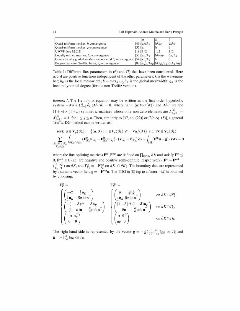
14 Ralf Hiptmair, Andrea Moiola and Ilaria Perugia
α β δ
Quasi-uniform meshes, h-convergence [46] a/khK bkhK dkhK
Quasi-uniform meshes, p-convergence [52] a b d
UWVF (see §2.2.2) [19] 1/2 1/2 1/2
Locally refined meshes, hp-convergence [53] ah/hK bh/hK dh/hK
Geometrically graded meshes, exponential hp-convergence [54] ah/hK b d
Polynomial (non Trefftz) basis, hp-convergence [82] aq2K/khK bkhK/qK dkhK/qK
Table 1: Different flux parameters in (6) and (7) that have been considered. Here
a,b,d are positive functions independent of the other parameters; k is the wavenum-
ber; hK is the local meshwidth; h = maxK∈ThhK is the global meshwidth; qK is the
local polynomial degree (for the non-Trefftz version).
Remark 1. The Helmholtz equation may be written as the first order hyperbolic
system −iku + ∑nj=1 ∂x j
(A( j)u) = 0, where u := (u;∇u/(ik)) and A( j) are the
(1+ n)× (1+ n) symmetric matrices whose only non-zero elements are A( j)1, j+1 =
A( j)j+1,1 = 1, for 1 ≤ j ≤ n. Then, similarly to [37, eq. (22)] or [39, eq. (5)], a general
Trefftz-DG method can be written as:
seek u ∈ Vp(Th) :=(u,σ) : u ∈Vp(Th),σ = ∇u/(ik)
s.t. ∀v ∈ Vp(Th)
∑K1,K2∈Th,
K1 6=K2
∫
∂K1∩∂K2
(Fin|K1
u|K1−Fin
|K2u|K2
)·(v|K1
−v|K2
)dS+
∫
∂Ω(Finu−g) ·vdS = 0
where the flux-splitting matrices Fin,Fout are defined on ∏K∈Th∂K and satisfy Fin ≤
0, Fout ≥ 0 (i.e. are negative and positive semi-definite, respectively), Fin +Fout =
( 0 n⊤KnK 0
) on ∂K, and FinK1
=−FoutK2
on ∂K1 ∩∂K2. The boundary data are represented
by a suitable vector field g=−Foutu. The TDG in (8) (up to a factor −ik) is obtained
by choosing:
FinK = Fout
K =
(−α 1
2n⊤
K12nK −βn⊗n⊤
)
(−(1−δ )ϑ δn⊤
K
(1−δ )n − δϑ n⊗n⊤
)
(−α n⊤
K
0 0
)
(α 1
2n⊤
K12nK βn⊗n⊤
)on ∂K ∩F I
h ,
((1−δ )ϑ (1−δ )n⊤
K
δn δϑ n⊗n⊤
)on ∂K ∩ΓR,
(α 0⊤
nK 0
)on ∂K ∩ΓD.
The right-hand side is represented by the vector g = − 1ik( 1−δ
δϑ−1nK)gR on ΓR and
g =−( αnK
)gD on ΓD.
A Survey of Trefftz Methods for the Helmholtz Equation 15
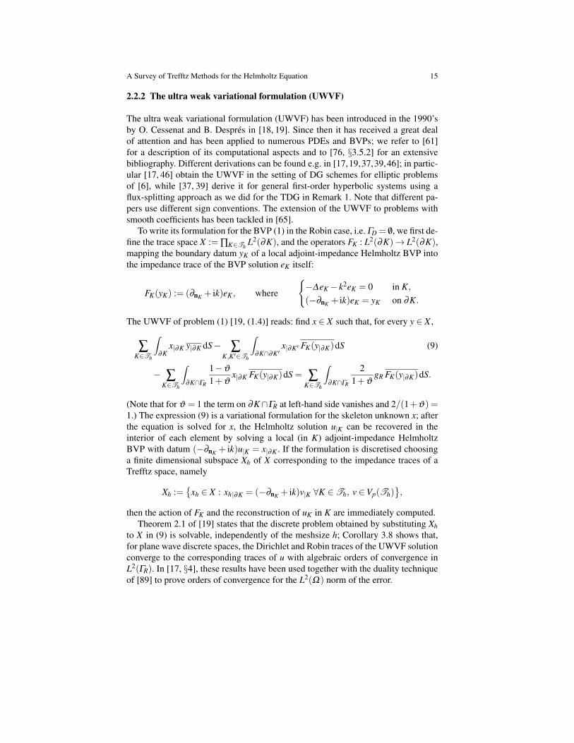
2.2.2 The ultra weak variational formulation (UWVF)
The ultra weak variational formulation (UWVF) has been introduced in the 1990’s
by O. Cessenat and B. Despres in [18, 19]. Since then it has received a great deal
of attention and has been applied to numerous PDEs and BVPs; we refer to [61]
for a description of its computational aspects and to [76, §3.5.2] for an extensive
bibliography. Different derivations can be found e.g. in [17,19,37,39,46]; in partic-
ular [17, 46] obtain the UWVF in the setting of DG schemes for elliptic problems
of [6], while [37, 39] derive it for general first-order hyperbolic systems using a
flux-splitting approach as we did for the TDG in Remark 1. Note that different pa-
pers use different sign conventions. The extension of the UWVF to problems with
smooth coefficients has been tackled in [65].
To write its formulation for the BVP (1) in the Robin case, i.e. ΓD = /0, we first de-
fine the trace space X := ∏K∈ThL2(∂K), and the operators FK : L2(∂K)→ L2(∂K),
mapping the boundary datum yK of a local adjoint-impedance Helmholtz BVP into
the impedance trace of the BVP solution eK itself:
FK(yK) := (∂nK+ ik)eK , where
−∆eK − k2eK = 0 in K,
(−∂nK+ ik)eK = yK on ∂K.
The UWVF of problem (1) [19, (1.4)] reads: find x ∈ X such that, for every y ∈ X ,
∑K∈Th
∫
∂Kx|∂K y|∂K dS− ∑
K,K′∈Th
∫
∂K∩∂K′x|∂K′ FK(y|∂K)dS (9)
− ∑K∈Th
∫
∂K∩ΓR
1−ϑ
1+ϑx|∂K FK(y|∂K)dS = ∑
K∈Th
∫
∂K∩ΓR
2
1+ϑgR FK(y|∂K)dS.
(Note that for ϑ = 1 the term on ∂K∩ΓR at left-hand side vanishes and 2/(1+ϑ) =1.) The expression (9) is a variational formulation for the skeleton unknown x; after
the equation is solved for x, the Helmholtz solution u|K can be recovered in the
interior of each element by solving a local (in K) adjoint-impedance Helmholtz
BVP with datum (−∂nK+ ik)u|K = x|∂K . If the formulation is discretised choosing
a finite dimensional subspace Xh of X corresponding to the impedance traces of a
Trefftz space, namely
Xh :=
xh ∈ X : xh|∂K = (−∂nK+ ik)v|K ∀K ∈ Th, v ∈Vp(Th)
,
then the action of FK and the reconstruction of uK in K are immediately computed.
Theorem 2.1 of [19] states that the discrete problem obtained by substituting Xh
to X in (9) is solvable, independently of the meshsize h; Corollary 3.8 shows that,
for plane wave discrete spaces, the Dirichlet and Robin traces of the UWVF solution
converge to the corresponding traces of u with algebraic orders of convergence in
L2(ΓR). In [17, §4], these results have been used together with the duality technique
of [89] to prove orders of convergence for the L2(Ω) norm of the error.

16 Ralf Hiptmair, Andrea Moiola and Ilaria Perugia
The UWVF has been recast as a DG method with Trefftz basis functions in
several different ways in [17, 37, 39, 46]. In particular, [46, Remark 2.1] shows
that the UWVF is a special case of the TDG formulation (8) for flux parameters
α = β = δ = 1/2. As a consequence, the orders of convergence in h and p proved
for the TDG on quasi-uniform meshes in [46, 52] carry over to the UWVF (with
suboptimal orders in h); on the other hand, the hp-type results of [53, 54] require
variable numerical flux parameters to cope with elements of different sizes (see Ta-
ble 1), so they do not apply to the UWVF. Thus, TDG can be understood as the
extension of the UWVF to non quasi-uniform meshes. Alternatively, in [88, §4.3,
5.2], the UWVF is employed on meshes refined towards solution singularities by
choosing Trefftz spaces on large elements and polynomial spaces on small ones. No
applications of the TDG combining mesh-dependent parameters and polynomial
spaces in small elements have been documented.
2.2.3 DG schemes with Lagrange multipliers
The DG schemes described so far enforce weak continuity between elements using
numerical fluxes, in the spirit of [6]. A different approach is to enforce continuity
using Lagrange multipliers. This was probably first proposed for Trefftz methods
in [63, §2.3], for the 1D Helmholtz equation.
This strategy has been followed in the discontinuous enrichment method (DEM),
introduced by C. Farhat, I. Harari and L.P. Franca in [32], combining a space of
piecewise-constant Lagrange multipliers on mesh interfaces with a discrete space
composed by sums of continuous piecewise polynomials and discontinuous plane
waves. Subsequently, in [33], the polynomial part of the trial space was dropped,
leaving a plane wave trial space and thus reducing to a Trefftz method; in this ver-
sion, the DEM was renamed discontinuous Galerkin method (DGM) and the La-
grange multipliers were approximated by oscillatory functions. This formulation
performed very well for test cases and was later extended to “higher order ele-
ments” (i.e. elements containing more plane waves) and other PDEs. We refer again
to [76, §3.5.3] for a comprehensive bibliography.
Here we briefly describe the formulation of the DGM following [33, §2]:
find (u,λ ) ∈ H1(Th)×W (Th) s.t.
ADGM(u,v)+BDGM(λ ,v) =∫
ΓR
gR vdS ∀v ∈ H1(Th),
BDGM(µ,u) =∫
ΓD
µ gD dS ∀µ ∈W (Th),
where
ADGM(w,v) : = ∑K∈Th
∫
K(∇w ·∇v− k2uv)dV +
∫
ΓR
ikϑ wvdS,
BDGM(µ,w) : = ∑K,K′∈Th
∫
∂K∩∂K′µ(w|K′ −w|K)dS+
∫
ΓD
µ wdS,

A Survey of Trefftz Methods for the Helmholtz Equation 17
W (Th) : =
(∏
K,K′∈Th
H−1/2(∂K ∩∂K′)
)×H−1/2(ΓD).
It is immediate to verify that the solution u to BVP (1) satisfies this formulation, and
that the multiplier λ represents the normal derivative of u on the mesh interfaces
and on ΓD. This formulation is then discretised by restricting it to finite dimensional
spaces Vp(Th)⊂ H1(Th) and Wp(Th)⊂W (Th). In the DEM of [32], Vp(Th) is the
direct sum of a continuous polynomial and a plane wave space, in the DGM of [33]
and subsequent papers only the plane wave part is retained, so Vp(Th)⊂ T (Th). The
volume degrees of freedom, i.e. those corresponding to Vp(Th), are then eliminated
by static condensation in order to reduce the computational cost of the scheme.
A stability and convergence analysis of the simplest version of the DGM (four
plane waves per element and piecewise-constant multipliers) is attempted in [4]:
for a Robin–Neumann BVP on a domain decomposed in rectangles, under a mesh
resolution condition, the scheme is shown to be well-posed, and a priori orders of
convergence are proved (in H1(Th) norm for the primal variable and in L2(Fh)for the multipliers), along with residual-type a posteriori error bounds. We are not
aware of any error analysis for the DGM method holding in more general situations
(e.g. more than four plane waves per elements, propagation direction not aligned to
the mesh, non-rectangular mesh elements).
A similar formulation, named hybrid-Trefftz finite element method, is described
in [99, §3.5] (deriving the functional in eq. (65) therein): the same form ADGM
above is used, while BDGM is substituted by BHT(µ,w) := −∫F I
hµ [[∇hw]]N dS −
∫ΓN
µ ∂nwdS, where now the multiplier µ approximates the Dirichlet trace of u, the
right-hand sides and the space W (Th) are changed accordingly. A further variant of
hybrid-Trefftz methods is presented in [109] and related papers.
Another DG method with Trefftz basis, called modified DG method (mDGM),
has been proposed in [48]. The Lagrange multipliers are double-valued on the in-
terfaces (differently from the DEM/DGM of [32,33]) and belong to ∏K∈ThL2(∂K \
ΓR). A two-step procedure is adopted. First, for each basis element λ ∈ L2(∂K \ΓR)of the discrete Lagrange multiplier space, a well-posed Helmholtz BVP on K with
impedance datum λ is solved in the local Trefftz space VpK(K) using the classical
H1(K)-conforming variational formulation. Second, these local solutions are com-
bined in a global LS formulation leading to a positive semi-definite system whose
unknowns are the Lagrange multipliers themselves. The mDGM was further im-
proved in [2] leading to the stable DG method (SDGM), which differs from the
mDGM in that the local impedance problems are solved with a least squares formu-
lation posed on ∂K, which gives local Hermitian matrices.
Lagrange multipliers are also used to tackle problems with discontinuous coeffi-
cients by means of the partition of unity method, see [73] and §2.5 below.

18 Ralf Hiptmair, Andrea Moiola and Ilaria Perugia
2.3 Weighted residual methods
Trefftz discretisations lend themselves well to weighted residual formulations: the
discrete solution is automatically a local solution of the PDE, only the residual on
interfaces (the jumps) and on the boundary (the mismatch with boundary conditions)
need to be enforced by multiplying them to suitable traces of test functions. The
choice of these traces leads to different variational formulations, the most developed
of which are the VTCR and the WBM described in the following. While it is simple
to design weighted residual methods, their error analysis is by no means easy, as
they do neither arise from integration by parts, nor from a minimisation principle.
An earlier weighted-residual Trefftz formulation is the weak element method of
[47], where the integral averages of Dirichlet and Neumann jumps on mesh faces
are set to zero (equivalently, test functions are constant on each mesh face).
We note that some of the earliest Trefftz schemes, e.g. the indirect approximation
of [22, eq. (35)], are of weighted-residual type, even though testing was confined to
the boundary of the domain only, see §2.4 below.
2.3.1 The variational theory of complex rays (VTCR)
The VTCR is a weighted residual Trefftz method introduced in the 1990’s by
P. Ladeveze and coworkers for problems arising in computational mechanics and
later extended to the Helmholtz case in [101]. Recent surveys are [70, 71, 100].
Several VTCR formulations, slightly different from each other, have been pre-
sented. A general VTCR formulation for the BVP (1) can be written as:
find uVTCR ∈Vp(Th) s.t. AVTCR(uVTCR,vhp) = ℓVTCR(vhp) ∀vhp ∈Vp(Th), where
AVTCR(u,v) := Im
∫
F Ih
([[u]]N · ∇hv− [[∇hu]]Nv
)dS (10)
+∫
ΓD
u∂nvdS+∫
ΓR
( C1
ikϑ(∂nu+ ikϑu)∂nv+C2(∂nu+ ikϑu)v
)dS
,
ℓVTCR(v) := Im
∫
ΓD
gD∂nvdS+∫
ΓR
( C1
ikϑgR ∂nv+C2 gR v
)dS
.
The formulations in [100, eq. (21)] and in [71, eq. (5)] correspond to the choice of
coupling parameters C1 = 1/2 and C2 = −1/2 (up to an overall factor k and using
Re−iz = Imz); that in [102, eq. (6)] to C1 = 1/2 and C2 = 1/2; that in [68,
eq. (4)] to C1 = 1 and C2 = 0. The choice of the coupling parameters does not affect
the consistency of the method as all terms in (10) are products of residuals (internal
jumps and boundary conditions) and traces of test functions. In some of the papers
cited, using Imab = − Imab∀a,b ∈ C, the conjugation is written on the trial,
rather than test, functions in some of the terms, without affecting the formulation.
The VTCR (and similarly the WBM) does not correspond to any of the classical
DG schemes listed in [6]. Indeed, to derive it from the elemental DG equation (5),

A Survey of Trefftz Methods for the Helmholtz Equation 19
one would need to choose numerical fluxes that, in the terminology of [6], are nei-
ther consistent (they do not equal the fields ∇u and u when applied to the exact
solution u itself) nor conservative (they are not single-valued on the interfaces).
Following [68, §2.2], it is possible to show that if absorption is present then the
VTCR is well-posed. More precisely, provided that C1 = 1, C2 = 0, Rek > 0 and
Imk2> 0, the VTCR bilinear form satisfies
AVTCR(v,v) =− Imk2‖v‖2L2(Ω)−
Rek
|k|2
∥∥∥ϑ−1/2∂nv
∥∥∥2
L2(ΓR)∀v ∈ T (Th),
thus the VTCR solution is unique in the Trefftz space and coercivity in L2(Ω) norm
holds (the analogous result for C1 =−C2 = 1/2 is proved in [71, Prop. 2]). However,
this does not extend to the setting we considered so far, i.e. propagating waves with
k ∈R: in this case it can easily be shown that AVTCR(v,v) = 0 for all v ∈ T (Th) such
that v = 0 on all elements adjacent to the Robin boundary ΓR and for any choice
C1,C2 ∈ C, thus well-posedness can not be ensured using a coercivity argument.
Following [71, Prop. 2], for C1 = 1/2,C2 =−1/2,k ∈ R, we have:
AVTCR(v,v) =−1
2
(1
k
∥∥∥ϑ−1/2∂nu
∥∥∥2
L2(ΓR)+ k
∥∥∥ϑ 1/2u
∥∥∥2
L2(ΓR)
)∀v ∈ T (Th),
thus (using Holmgren’s theorem [20, Th. 2.4]) uniqueness of the solution of (10) is
proved if all mesh elements are adjacent to ΓR. For more general cases, coercivity
appears to be too strong an argument. We conjecture that discrete inf-sup conditions
might be a more viable way for proving well-posedness of the VTCR.
Section 3 of [71] considers the application of the VTCR formulation, cor-
rected with suitable volume terms, with non-Trefftz (piecewise-polynomial) discrete
spaces. This variation is termed weak Trefftz and analysed therein.
2.3.2 The wave based method (WBM)
The WBM is a weighted residual Trefftz method, analogous to the VTCR, first
introduced in the dissertation of W. Desmet [26] and later extended to a wide variety
of engineering applications, mainly in the realm of vibro-acoustics. Recent reviews
of the state of the art of the research on the WBM can be found in [24, 27]. The
discrete space typically used together with the WBM is composed of propagating
and evanescent plane waves, as outlined in §3.2.
The basic variational formulation of the WBM applied to BVP (1), translating
§4.1.4 of [27] to our notation and multiplying all terms by (−ik), reads
find uWBM ∈Vp(Th) s.t. AWBM(uWBM,vhp) = ℓWBM(vhp) ∀vhp ∈Vp(Th), where
AWBM(u,v) :=∫
F Ih
(2[[∇hu]]Nv+
ik
Zint
[[u]]N · [[v]]N
)dS
+∫
ΓR
(∂nu+ ikϑu
)vdS−
∫
ΓD
u∂nvdS

20 Ralf Hiptmair, Andrea Moiola and Ilaria Perugia
ℓWBM(v) :=∫
ΓR
gR vdS−∫
ΓD
gD ∂nvdS,
where Zint is an interior coupling factor. In some works, a slightly different formula-
tion is used, e.g. in [98, eq. (81)] different terms are used on the internal interfaces.
We are not aware of any rigorous stability or error analysis of the WBM formulation.
2.4 Single-element direct and indirect Trefftz methods
Despite most schemes described so far were introduced not earlier than mid 1990’s,
a lot of research on Trefftz methods has been carried out since the late 1970’s by
I. Herrera, J. Jirousek, A.P. Zielinski, O.C. Zienkiewicz and numerous co-workers,
mainly for static elasticity problems. General reviews of these works are in [67,121];
the Helmholtz case is described in detail in [22]. A major difference between these
methods and those we described in the previous sections is that in many instances of
the former ones no mesh is introduced on the domain Ω , so that the unknowns are
defined on ∂Ω only. For this reason, these Trefftz methods more closely resemble
standard boundary element methods rather than finite element schemes.
There are two main classes of these Trefftz methods: direct and indirect. (We use
the terms “direct” and “indirect” as in [22,67] and [98, §5.1].) We describe them for
a modification of BVP (1) where we drop the Robin boundary ΓR and we consider
instead a Neumann boundary portion ΓN with boundary condition ∂nu = gN .
The indirect method is the simplest kind of weighted residual scheme:
∫
ΓD
u∂nvdS−∫
ΓN
∂nuvdS =∫
ΓD
gD ∂nvdS−∫
ΓN
gNvdS, (11)
(see [22, eq. (35)] for sound-hard scattering problems in unbounded domains, [98,
eq. (47)], [121, eq. (16)], [67, eq. (16), (26)]). For Dirichlet exterior problems this
is also the method of [8, §3]. In most references the test function is not conjugated.
We note that the indirect method is nothing else than the WBM of §2.3.2 posed
on a single element, i.e. Th = Ω and F Ih = /0. In the indirect method, the trial
functions approximating u are global solutions of the Helmholtz equation on the
whole of Ω ; on the other hand the test function v only needs to be defined on ∂Ω .
If the Trefftz test and trial spaces coincide, then the obtained stiffness matrix is
symmetric (by Green’s second identity). If the signs of the terms on ΓN are changed,
as in [67, eq. (22)], a non-symmetric formulation is obtained.
Subtracting from (11) the second Green’s identity∫
∂Ω (u∂nv − ∂nuv)dS = 0,
which holds for all Helmholtz solutions u and v in Ω , we derive the direct method:
∫
ΓD
∂nuvdS−∫
ΓN
u∂nvdS =∫
ΓD
gD ∂nvdS−∫
ΓN
gN vdS, (12)
(see [22, eq. (42)], [98, eq. (50)]). The direct method for the Dirichlet problem may
be viewed as the TDG of §2.2.1 with α = 0 posed on a single element K = Ω .
A Survey of Trefftz Methods for the Helmholtz Equation 21
Conversely to the indirect method, consistency of (12) is guaranteed only if the test
functions are Helmholtz solutions in Ω , while the trial functions might be defined
(and often are) on ∂Ω only, for better computational efficiency; the solution is then
evaluated in Ω with a representation formula in a post-processing step as for BEMs.
The stiffness matrix arising from the direct formulation (12) is the transpose to that
of the indirect method (11). Theorem 6.44 in [105] gives sufficient conditions for
the well-posedness of the direct method. Theorem 7.19 in [21] proves that, for well-
posed Dirichlet problems with H1(∂Ω) data, if the Neumann traces of the trial space
coincide with the Dirichlet traces of the test space, then the direct method is well-
posed and computes the best approximation of the exact solution in L2(∂Ω) norm.
If Ω is unbounded, the direct and the indirect methods can still be used choosing
discrete functions that satisfy Sommerfeld radiation condition; however in (12) the
conjugation on the test function must be dropped to preserve consistency. In this
case, if a multipole basis is used, Waterman’s null-field method is obtained, see [78,
Ch. 7], which is a special instance of the T-matrix method [78, §7.9]. (Note that [92]
uses the name null-field method for the indirect method with non-conjugated test
functions, and Cremer equations for the same with conjugated test functions.)
For a special choice of Trefftz test functions v indexed by a complex param-
eter (see the last paragraph of §3.2), method (12) is called “global relation” and
is the variational formulation at the heart of the Fokas transform method, see [23,
eq. (2)], [105, eq. (6.142–143)] or [21, eq. (7.156)]. In this context, this formulation
is typically discretised using piecewise-polynomial (on ∂Ω ) trial functions, even
though Trefftz functions may be used as well.
2.5 Non-Trefftz methods with oscillatory basis functions
The main reason for the success of Trefftz methods in the context of time-harmonic
wave problems is that the oscillatory basis functions may offer much better approx-
imation properties than piecewise polynomials used in standard FEMs. On the other
hand, similar approximation can also be achieved if the discrete functions are not
exact local solution of the PDE to be discretised, but are are only “approximate so-
lutions”. If basis functions of this kind are used, the Trefftz formulations described
in the previous sections cannot be employed as they stand, because the residual in
the elements will not vanish any more and consistency will fail.
Approximate Trefftz functions are especially attractive for problems with smooth-
ly varying material parameters, where no analytic Trefftz function might be known.
Trefftz formulations, possibly with additional volume terms, can be used with ba-
sis functions that are solutions of the equation only up to a certain order; see
[15, 65, 110], where this idea is pursued for DG, UWVF and DEM formulations.
In the following we briefly discuss a few methods that have been proposed em-
ploying oscillatory and k-dependent basis functions that are not Trefftz.
A very well-known scheme of this kind is the partition of unity method (PUM or
PUFEM), introduced by I. Babuska and J.M. Melenk in the mid 1990’s, see e.g. [81].

22 Ralf Hiptmair, Andrea Moiola and Ilaria Perugia
The PUM combines the approximation properties of Trefftz functions with the stan-
dard variational formulation of the problem, e.g. for the BVP (1) with ΓD = /0
∫
Ω
(∇hu ·∇hv− k2uv
)dV +
∫
ΓR
ikϑuvdS =∫
ΓR
gR vdS ∀v ∈ H1(Ω). (13)
This requires the use of H1(Ω)-conforming trial and test functions, thus continuity
on interfaces needs to be enforced strongly, which is not viable in Trefftz spaces.
The PUM uses as basis a set of Trefftz functions multiplied to a partition of unity
defined on a FEM mesh, e.g. piecewise linear/multilinear polynomial FEMs on sim-
plicial/tensor elements. Theorem 2.1 in [81] ensures that the trial space obtained
enjoys the same approximation properties of the Trefftz space employed. If a p-
dimensional local Trefftz space is used in each element, together with a piecewise
linear/multilinear partition of unity, the total number of degrees of freedom used
equals p times the number of mesh vertices, while for a similar Trefftz method on
the same mesh (providing comparable accuracy) it would equal p times the num-
ber of mesh elements; this means that on tensor meshes almost the same number
of DOFs would be employed by the two methods, while on triangles and tetrahedra
a saving of a factor up to two or six, respectively, can be achieved by the PUM. A
shortcoming of the PUM is that the formulation (13) is not sign-definite and its well-
posedness requires a scale resolution condition, while this is not needed for some
Trefftz schemes such as the TDG/UWVF presented in §2.2.1 and §2.2.2. Differently
from Trefftz schemes, the implementation of the PUM requires the computation of
volume integrals; moreover, the numerical integration of the PUM basis functions
may be more expensive than that of genuine Trefftz functions, see §4.1.
The PUM for the Helmholtz and other frequency-domain equations was further
developed by R.J. Astley, P. Bettes, A. El Kacimi, O. Laghrouche, M.S. Mohamed,
E. Perrey-Debain, J. Trevelyan and collaborators, see e.g. [72, 96]. When a PUM
and a standard FEM discrete spaces are combined, e.g. using formulation (13), the
method obtained is termed generalised finite element method (GFEM); e.g. [108]
employs high-order tensor product polynomials summed to products of plane waves
and bilinear functions. In problems with discontinuous wavenumber k, the PUM can
be applied by coupling the homogeneous regions by means of Lagrange multipliers
as in [73]; this is not necessary as formulation (13) holds on the whole domain, but
enhance the accuracy as in each subdomain only basis functions oscillating with the
correct local wavelength are used. In [51] and related papers, the trigonometric finite
wave elements (TFWE) is described: the PUM is used with special basis functions
adapted to waveguides, lasers and geometries with a single dominant wave propa-
gation direction. The finite ray element method of [79] consists in the use of a PUM
basis in a first order system of least squares (FOSLS) formulation; as the unknown
is constituted by both u and its gradient, more unknowns are needed but the system
matrix is Hermitian. Finally, in the hybrid numerical asymptotic method of [42], the
PUM space is constructed by multiplying nodal finite elements to oscillating func-
tions whose phases are derived from geometrical optics (GO) or geometrical theory
of diffraction (GTD), e.g. by solving the eikonal equation, cf. §4.2.

A Survey of Trefftz Methods for the Helmholtz Equation 23
Plane wave bases have been combined in [97] with the virtual element method
(VEM) framework [11], in order to design a high-order, conforming method for the
Helmholtz problem, in the spirit of the PUM, but allowing for general polytopic
meshes. The main ingredients of the resulting PW-VEM are (i) a low frequency
space made of low order VEM functions, which do not need to be explicitly com-
puted in the element interiors, (ii) a proper local projection operator onto a high-
frequency space made of plane waves, and (iii) an approximate stabilisation term.
The implementation of the PW-VEM does not require computation of volume in-
tegrals, and no quadrature formulas are required for the assembly of the stiffness
matrix, for meshes with flat interelement boundaries.
The hybridizable DG method of [91] employs two discontinuous discrete spaces
(one scalar and one vector) and a space of Lagrange multipliers on the mesh in-
terfaces. Though Trefftz spaces might be used with this formulation, the authors
consider basis functions constructed as products of polynomials and geometrical
optics-based oscillating functions, similar to those in [42] but discontinuous.
A Trefftz approach has been proposed in the context of finite difference schemes
in the flexible local approximation method (FLAME) by I. Tsukerman, see e.g. the
comprehensive review [113]. In the FLAME, the Taylor expansion of the solution
to be approximated used to define classical finite difference schemes is substituted
by an expansion in a series of Trefftz basis functions, leading to better accuracy.
Oscillatory basis functions have been successfully used in boundary element
methods, in particular for scattering problems, see the review on the hybrid numer-
ical-asymptotic BEM (HNA-BEM) [20], the plane-wave basis boundary elements
[96, §3] and the extended isogeometric boundary element method (XIBEM) [93].
3 Trefftz discrete spaces and approximation
Given a Trefftz variational formulation of a BVP, as those in §2, the definition of a
Trefftz finite element method is completed by the choice of a discrete space
Vp(Th) =
v ∈ T (Th) : v|K ∈VpK(K)⊂ T (Th),
where VpK(K) is a pK-dimensional space of functions v on K such that ∆v+k2v= 0.
We describe next the main features of the most common local Trefftz spaces VpK(K);
we do not consider Lagrange multiplier spaces on mesh faces for the methods in
§2.2.3. The discussion of the conditioning properties of the basis functions described
and of the techniques for their numerical integration is postponed to §4.
24 Ralf Hiptmair, Andrea Moiola and Ilaria Perugia
3.1 Generalised harmonic polynomials (GHPs)
Generalised harmonic polynomials are smooth Helmholtz solutions that are separa-
ble in polar and spherical coordinates in 2D and 3D, respectively, i.e. circular and
spherical waves (also called Fourier–Bessel functions or Fourier basis). The local
spaces VpK(K) are defined as follows:
2D: VpK(K) =
v : v(x) =
qK
∑ℓ=−qK
αℓ Jℓ(k |x−xK |)eiℓθ , αℓ ∈ C
,
3D: VpK(K) =
v : v(x) =
qK
∑ℓ=0
ℓ
∑m=−ℓ
αℓ,m jℓ(k |x−xK |)Y mℓ
( x−xK
|x−xK |
), αℓ,m ∈ C
,
where xK ∈ K (e.g. is the mass centre of K), θ is the angle of x in the local polar
coordinate system centred at xK , Jℓ is the Bessel function of the first kind and order
ℓ, Y mℓ ℓm=−ℓ is a basis of spherical harmonics of order ℓ (see, e.g. [85, eq. (B.30)]),
and jℓ is the spherical Bessel function defined by jℓ(z) =√
π2z
Jℓ+ 12(z). The space
dimension pK is given by pK = 2qK +1 in 2D and by pK = (qK +1)2 in 3D. We call
qK , the maximal index of the (spherical) Bessel functions used, the “degree” of the
GHP space, as it plays the same role of the polynomial degree in the approximation
theory. A particular feature of GHP spaces is that they are hierarchical.
The name “generalised harmonic polynomials” was coined in [80] and comes
from the fact that they are images of harmonic polynomials under the operator that
maps harmonic functions into Helmholtz solutions, in the framework of Vekua–
Bergman’s theory [12, 114] (see also [50, 87]). The same theory allows to transfer
approximation results for harmonic functions by spaces of harmonic polynomials
into results on the approximation of Helmholtz solutions by GHPs. The density of
GHPs in a space of Helmholtz solutions was proved in [50, Th. 4.8] and [114, §22.8].
Approximation estimates in two dimensions were first proved in [28, Th. 6.2] (in
L∞ norm) and in [80] (in Sobolev norms), and later sharpened and extended to three
dimensions in [86]. We summarise here the estimates of [86, Th. 3.2].
Let D ∈Rn, n = 2,3, be a bounded, open set with Lipschitz boundary and diame-
ter hD, containing BρhD(xD) (the ball centred at some xD ∈ D and with radius ρhD),
and star-shaped with respect to Bρ0hD(xD), where 0 < ρ0 ≤ ρ ≤ 1/2. Assume that
u ∈ Hs+1(D), s ∈ N, satisfies ∆u+ k2u = 0 in D and define the k-weighted Sobolev
norm ‖u‖ j,k,D := (∑jm=0 k2( j−m) |u|2m,D)
1/2, j ∈ N, where |·|m,D is the Sobolev semi-
norm of order m on D.
i) If n = 2 and D satisfies the exterior cone condition with angle λDπ [86, Def. 3.1]
(λD = 1 if D is convex), then for every L ≥ s there exists a GHP QL of degree at
most L such that, for every j ≤ s+1, it holds
‖u−QL‖ j,k,D ≤C(1+(hDk) j+6
)e
34 (1−ρ)hDk
(( log(L+2)
L+2
)λD
hD
)s+1− j
‖u‖s+1,k,D ,

A Survey of Trefftz Methods for the Helmholtz Equation 25
where the constant C > 0 depends only on the shape of D, j and s, but is inde-
pendent of hD, k, L and u.
ii) If n = 3, there exists a constant λD > 0 depending only on the shape of D, such
that for every L ≥ maxs,21/λD there exists a GHP QL of degree at most L such
that, for every j ≤ s+1, it holds
‖u−QL‖ j,k,D ≤C(1+(hDk) j+6
)e
34 (1−ρ)hDkL−λD(s+1− j)h
s+1− jD ‖u‖s+1,k,D ,
where the constant C > 0 depends only on the shape of D, j and s, but is inde-
pendent of hD, k, L and u.
The main difference between the two results is that the positive shape-dependent
parameter λD entering the exponent of L (thus the p-convergence order) is explicitly
known in 2D (it depends on the largest non-convex corner of D) but not in 3D.
Exponential convergence of the GHP approximation of Helmholtz solutions that
possess analytic extension outside D were proved in [85, Prop. 3.3.3] and improved
in 2D in [54], based upon the corresponding result for harmonic functions of [55].
Roughly speaking, the error is bounded by a negative exponential of the form
C exp(−bL) ∼ C exp(−bp1/(n−1)D ), while classical bounds for polynomials achieve
at most C exp(−bp1/n
D ), since the dimension pD of the GHP space of order L is
O(Ln−1), while the dimension pD of the polynomial space of degree L is O(Ln).Thus, Trefftz methods based on GHPs (and similarly on PWs) can achieve better
asymptotic order than standard schemes; however the value of the positive coeffi-
cients b,C and their dependence on the BVP and discretisation are not entirely clear.
Approximation estimates in the (discontinuous) spaces Vp(Th) immediately fol-
low form the local approximation estimates with D = K, for all K ∈ Th. In case
of (H1-conforming) partition of unity spaces enriched with GHPs, global estimates
follow from combining the local estimates with [81, Th. 2.1].
GHPs have been proposed in numerous Trefftz formulations: LS [89, 107],
UWVF [77], VTCR [68], hybrid-Trefftz [99, eq. (62)], direct and indirect single-
element schemes [22, 121], HELS [117], MPS [16, 36].
3.2 Plane waves (PWs)
Plane waves probably constitute the most common choice of Trefftz basis functions.
In this case, the local space VpK(K) is defined by
VpK(K) =
v : v(x) =
pK
∑ℓ=1
αℓ eikdℓ·(x−xK), αℓ ∈ C
, (14)
where dℓpK
ℓ=1 ⊂ Rn, |dℓ| = 1, are distinct propagation directions. To obtain iso-
tropic approximations, in 2D, uniformly-spaced directions on the unit circle can be
chosen (i.e. dℓ = (cos(2πℓ/pK),sin(2πℓ/pK))); in 3D, [103] and [94] provide di-

26 Ralf Hiptmair, Andrea Moiola and Ilaria Perugia
rections that are “almost equally spaced” (see [1, §3.4] for a simpler version). In
these cases, the PW spaces are not hierarchical. However, one of the potential bene-
fits of PW approximations is the possibility to depart from the isotropic case and to
adapt the basis propagation directions to the specific BVP at hand and to different
elements, either a priori or a posteriori, see §4.2.
The linear independence of arbitrary sets of plane waves (and of their traces)
is proved in [1, 21]. PW bases whose linear independence does not degenerate for
small values of khK were introduced in [46, §3.1] in 2D and in [86, §4.1] in 3D (see
also [85, §3.4.1]) for analysis purposes. These stable PW bases converge to GHP
bases in the low-frequency limit [86, p. 815]. The existence of these stable bases,
which is instrumental to the derivation of approximation estimates for Helmholtz
solutions in PW spaces in [86], is guaranteed, provided that the set of directions
dℓpK
ℓ=1 constitutes a fundamental system for certain harmonic polynomials. In 2D,
any choice of pK = 2qK + 1 distinct directions, qK being the maximal degree of
the considered harmonic polynomials, guarantees this property. In 3D, sufficient
conditions on pK = (qK +1)2 directions are stated in [86, Lemma 4.2].
Approximation estimates in PW spaces can be derived from similar bounds for
GHPs such as those in §3.1. In [80, Ch. 8], GHPs were approximated by PWs
by approximating their smooth Herglotz kernel with delta functions, leading to p-
estimates in 2D, while in [86] the Jacobi–Anger expansion was used to link PWs
and GHPs in 2D and 3D. Theorems 5.2 and 5.3 of [86] (see also [85, §3.5]) show
that Helmholtz solutions of given Sobolev regularity can be approximated in PW
spaces with hp-estimates similar to those shown in §3.1 for GHPs. For PWs, these
estimates hold with L = qK , so that qK plays the role of a “degree” for the consid-
ered PW space. As mentioned, for these bounds to hold in 3D, the PW directions
have to satisfy some further conditions. A different derivation of h-approximation
estimates based on a Taylor argument can be found in [19, Th. 3.7]. In [95], the
PW approximation of Helmholtz solutions on the unit disc is analysed in detail,
together with the conditioning of different linear systems used for its computation
(least squares and collocation for a Dirichlet problem on the disc) and the implica-
tions on the accuracy of the approximation computed in finite-precision arithmetic.
We refer again to [54, §5.2] for the exponential convergence in 2D of PW approx-
imations of analytic Helmholtz solutions (see also [85, Rem. 3.5.8] which holds in
2D and 3D).
Similar to PWs are the evanescent waves: the basis elements have the same ex-
pression v(x) = eikd·x but with a more general d ∈Cn, d ·d = 1. If d = dR+ idI , with
dR,dI ∈ Rn, then v oscillates in the direction dR (with wavenumber k|dR| ≥ k) and
decays exponentially in the orthogonal direction dI (i.e. |v(x)| = e−kdI ·x). Evanes-
cent waves are used in combination with plane waves to approximate interface prob-
lems in the DEM [111] and the UWVF [77], and to represent outgoing waves in a
2D unbounded half-strip of the form a < x < b,y > c in [21, 119].
A special combination of propagative and evanescent waves is typically used in
the WBM. We describe a 2D version of this space as in [24, eq. (14)–(21)] (see
[27, §4.1] for 3D). This space is not invariant under rotation but depends on the
choice of the Cartesian axes. For a mesh element K, we fix a truncation parameter

A Survey of Trefftz Methods for the Helmholtz Equation 27
N > 0 (typically 1 ≤ N ≤ 6) and define Lx := sup(x1,y1),(x2,y2)∈K |x1 − x2| and Ly :=sup(x1,y1),(x2,y2)∈K |y1 − y2| as the edge lengths of the smallest rectangle containing
K and aligned to the Cartesian axes. Two sets of basis functions are used:
cos(kx jx)e±i√
k2−k2x j y
, kx j :=jπ
LKx
, j = 0, . . . ,⌊NkLKx /π⌋,
e±i√
k2−k2y j x
cos(ky jy), ky j :=jπ
LKy
, j = 0, . . . ,⌊NkLKy /π⌋,
for a total dimension pK = 4+ 2(⌊NkLx/π⌋+ ⌊NkLy/π⌋). Each basis function is
half the sum of two plane (or evanescent) waves, symmetric to one another with
respect to the x or y axis: e.g. cos(kx jx)exp(i√
k2 − k2x jy) =
12(eikd+x j ·x + e
ikd−x j ·x),
with d±x j := (±kx j/k,
√1− (kx j/k)2). A maximum of 4+ 2(⌊kLx/π⌋+ ⌊kLy/π⌋)
basis functions are propagative PWs, this number designed to keep the conditioning
under control. If N > 1, then roughly a fraction (N − 1)/N of the total basis func-
tions are evanescent waves decaying in a direction parallel to one of the Cartesian
axes. Refinement is obtained by increasing N: for N ≤ 1 only propagative waves are
present, for higher values evanescent waves are introduced.
In 2D, both evanescent and plane waves may be written as exp k2(i(ν +1/ν)x+
(ν −1/ν)y= expik(xsinθ + ycosθ, parametrised by ν ∈ C or θ ∈ C with ν =eiθ ; these waves constitute the test space (but usually not the trial) for the Fokas
method in [23, 105] and [21, §7.3.4] (see also §2.4).
3.3 Fundamental solutions and multipoles
Fundamental solutions and multipoles are Helmholtz solution in the complement
of a point and satisfy Sommerfeld radiation condition (limr→∞ rn−1
2 ( ∂u∂ r
− iku) = 0,
where r = |x|). They are particularly useful to define Trefftz spaces on unbounded
elements, e.g. for for scattering problems.
If the local spaces are spanned by fundamental solutions, simple sources are
located at distinct poles xℓ in the complement of K:
2D : VpK(K) =
v : v(x) =
pK
∑ℓ=1
αℓ H(1)0 (k |x−xℓ|), αℓ ∈ C
,
3D : VpK(K) =
v : v(x) =
pK
∑ℓ=1
αℓe−ik|x−xℓ|
|x−xℓ|, αℓ ∈ C
,
where H(1)0 is the Hankel function of the first kind and of order 0. Different a priori
or a posteriori strategies are used to fix the location of the poles, see §2.1.1 and the
references cited therein. As the distance of the points xℓ from K increases, these ba-

28 Ralf Hiptmair, Andrea Moiola and Ilaria Perugia
sis functions approach plane waves, so they permit flexibility not only in the choice
of the propagation directions but also in the wavefront curvature.
Apart from the MFS and its modifications (see §2.1.1 and [1, 9, 10, 31, 92, 120]),
spaces of fundamental solutions have been used in connection to the UWVF (see
[58], where ray-tracing is used to determine the poles, and [57]).
Theorem 6 of [104] ensures that Helmholtz solutions in K can be approximated
in Holder norms by fundamental solutions centred at any “embracing boundary” in
2D and 3D, under weak assumptions on the regularity of ∂K. We are not aware of
any result providing orders of convergence.
An alternative approach consists in choosing local spaces generated by multipole
expansions, where multiple sources with increasing order are located at a single pole
x0 (or only at few poles):
2D : VpK(K) =
v : v(x) =
qK
∑ℓ=−qK
αℓ H(1)ℓ (k |x−x0|)eiℓθ , αℓ ∈ C
,
3D : VpK(K) =
v : v(x) =
qK
∑ℓ=0
ℓ
∑m=−ℓ
αℓ,m h(1)ℓ (k |x−x0|)Y m
ℓ
( x−x0
|x−x0|
), αℓm ∈ C
,
where H(1)ℓ (h
(1)ℓ ) are Hankel functions (spherical Hankel functions, respectively) of
the first kind and order ℓ. As for the GHPs in §3.1, θ is the angle of x in the local
coordinate system centred at x0, which is located in the complement of K, and the
space dimension is pK = 2qK +1 in 2D and pK = (qK +1)2 in 3D. According to [10,
Rem. 2.2], fundamental solutions lead to more stable methods than multipoles.
Multipole spaces have been used in connection to LS schemes [90, 107], WBM
[24, eq. (23)], [27, §4.1.2], hybrid-Trefftz [99, eq. (63)], HELS [117], source simula-
tion techniques [92], null-field [78] and single-element schemes [8,22,121]. In [49]
and related papers, some 2D multipoles with suitably chosen index ℓ (not necessar-
ily integer) are used on infinite sectors, in such a way to ensure continuity of discrete
functions across rays; this might be more efficient than full multipole spaces for so-
lutions with a preferred propagation direction.
3.4 Other basis functions
Other discrete Trefftz spaces have been proposed in literature for use with the vari-
ous approaches covered in §2.
In 2D, corner waves such as Jℓ/α(k|x|)sin(ℓθ/α), with ℓ ∈ N and 0 < α < 2,
capture the behaviour of Helmholtz solutions near a domain corner of angle πα .
They have been used e.g. in the WBM [25], in LS methods [10, 107, 119] and in
the MPS [16, 36]. In [120], they are used on tips of 1D screens to represent the
strong singularities of the solution in a non-Lipschitz domain. Theorem 6.3 of [28]
uses Vekua–Bergman theory to give orders of convergence for the approximation

A Survey of Trefftz Methods for the Helmholtz Equation 29
of singular functions by spaces of corner waves and GHPs (see also [10, §5] and
references therein). We are not aware of any use of similar functions in 3D.
The wave band functions, introduced in the VTCR context [101], are Herglotz
functions with piecewise-constant kernel, e.g.∫ b
a eik(xcosθ+ysinθ) dθ in 2D.
In the presence of a circular hole, suitable combinations of Hankel and Bessel
functions a priori fulfil homogeneous boundary conditions [107, eq. (13)].
If the wavenumber varies inside an element, the basis functions described so
far do not lead to Trefftz methods. In case of linearly variable wavenumber, Airy
functions can be used to construct Trefftz spaces [110]. In [64,65] generalised plane
waves in the form eP(x), for suitable polynomials P, are introduced and analysed in
a UWVF setting: they solve a perturbed Helmholtz problem and converge with high
orders in hK . Similar “almost-Trefftz” waves are used in [43] and named oscillated
polynomials. Modulated plane waves, i.e. products of PWs and polynomials, are
the basis functions of the DG method of [14, 15]; as they are only “approximately
Trefftz”, volume terms appear in the formulation.
Products of (continuous) low-order polynomials and PWs or GHPs constitute the
basis of the PUM [51,73,81,96,108], while products of polynomials and oscillating
functions derived from high-frequency asymptotics are basis elements in [42, 91].
4 Further topics
4.1 Assembly of linear systems
All the Trefftz finite element methods for (1) discussed in §2 give rise to dense
or sparse linear systems of equations. Entries of coefficient matrices are obtained
by integrating products of (derivatives of) trial and test functions over bounded d-
dimensional sub-manifolds of Ω , d < n. The stable and accurate (approximate) eval-
uation of these integrals is a key implementation issue.
Among all Trefftz approximation spaces and associated bases presented in §3,
plane waves (PWs) eikd·x (either propagative with d ∈ Rn or evanescent with d ∈
Cn) are exceptional, because they allow a closed-form evaluation of their integrals
over any flat sub-manifold with piecewise flat/straight boundary. For instance, in all
variants of PW-based Trefftz methods on polyhedral meshes in 3D, expressing mesh
faces by 2D parametrisations, we eventually encounter integrals of the form
∫
Fexp(w ·x)dV, F ⊂ R
2 a bounded polygon, w ∈ C2 constant. (15)
Then we can take the cue from [38, §2.1] or [29, §4] and apply integration by parts
in order to reduce (15) to integrals over the straight edges e1,e2, . . .eq, q ∈ N of F :
∫
Fexp(w ·x)dV =
1
w ·w
∫
Fw ·∇exp(w ·x)dV =
q
∑ℓ=1
w ·nℓ
w ·w
∫
eℓ
exp(w ·x)ds,

30 Ralf Hiptmair, Andrea Moiola and Ilaria Perugia
where nℓ is the exterior normal at eℓ. In turns, as in [44, Ch. 2], if eℓ = [a,b],a,b ∈R
2, we find,∫
eℓexp(w ·x)ds = exp(w ·a)|b−a|ψ(w ·(b−a)), where ψ(z) :=
(exp(z)−1)/z. Of course, a numerically stable implementation of this function for
small arguments is essential1. This approach can be generalised to yield analytic for-
mulas for computing integrals of products of PWs times polynomials, see [29, 38],
with increased computational effort, however.
Approximate evaluation of the integrals becomes inevitable for all choices of Tr-
efftz basis functions other than PWs, and even for a PW basis on meshes with curved
elements. Then Gauss–Legendre numerical quadrature seems to be the most widely
used option. However, the integrands may be oscillatory, which delays the onset of
(exponential) convergence of the quadrature error until the number of quadrature
points surpasses a threshold roughly proportional to the ratio of the local mesh size
and the wavelength. This leads to higher computational cost per degree of freedom
for larger values of khK . One may think of using special quadrature rules for os-
cillatory integrals, as derived, for instance, in [62]. Those avoid an increase in the
number of quadrature points for growing spatial frequency of the oscillations, but
unfortunately require precise knowledge of the oscillatory term in the integrand.
4.2 Adaptive Trefftz methods
Besides classical h-, p- or hp-adaptivity, Trefftz methods offer scope for more so-
phisticated adaptive strategies consisting in the choice of specific basis functions for
different BVPs and in different mesh elements, either a priori or a posteriori.
The main strand of a priori adaptive Trefftz methods falls into the category of
hybrid numerical-asymptotic methods. High-frequency limit models, such as ray
optics or geometric theory of diffraction (GTD), guide the selection of local Trefftz
spaces in the individual cells of a mesh. In a non-Trefftz PUM framework this idea
was pursued in [42], and within the hybridizable DG method in [91], in both cases
for 2D acoustic scattering at a smooth sound-soft object. In these works, local phase
factors x 7→ exp(ikS(x)) derived from reflected and diffracted waves multiply stan-
dard continuous nodal basis functions, in [42], or local polynomials, in [91], thus
generating a basis for (local) trial spaces.
The policy of incorporating local directions of rays is particularly attractive for
PW-based methods, because PW basis functions naturally encode a direction of
propagation. For problems where excitation is due to an incident PW and mate-
rial properties are piecewise constant, ray tracing and related techniques [91, §3.2]
based on geometric optics (specular reflection and Snell’s law of refraction at ma-
terial interfaces) can provide information about the local orientation of wave fronts
for k → ∞. PWs matching the found ray directions are then used to build local bases,
either exclusively or augmented by a reduced set of generalised harmonic polyno-
mials (GHPs) or “equi-spaced” PWs.
1 A stable algorithm for point evaluations of ψ even for arguments close to 0 is provided by the
MATLAB function expm1.
A Survey of Trefftz Methods for the Helmholtz Equation 31
This idea for TDG was first outlined and tested in [14] and further elaborated
and extended in [58, Ch. 5] (for UWVF). In the latter work, in an attempt to resolve
curved wave fronts and take into account diffracted waves from corners, also Han-
kel functions x 7→ H10 (k|x− y∗|) with y∗ outside a mesh cell have been proposed
as local basis functions. Approximation of curved wave fronts deduced from GTD
corrections is also attempted in [15]. There the authors move beyond Trefftz meth-
ods and use DG with trial spaces of polynomially modulated PWs, which are more
suitable for approximating propagating circular waves.
In simple 2D situations with convex smooth or polygonal scatterers and incident
plane wave, overall accuracy seems to benefit substantially from a priori directional
adaptivity. However, if there are more than only a few dominant wave directions
as in the case of more complicated geometries, trapping of waves, dark zones and
shadow boundaries, current directional adaptivity soon meets its limitations. On the
other hand, this strategy appears as the most promising way to achieve k-uniform
accuracy with numbers of degrees of freedom that remain k-uniformly bounded
or display only moderate growth as k → ∞. The potential of this idea has been
strikingly demonstrated in the case of BEM for 2D scattering problems [20].
A posteriori directional adaptivity seeks to extract information about dominant
wave directions from intermediate approximations of u. A refine-and-coarsen strat-
egy is embraced in [14]. In each step of the adaptive cycle it first computes a PWDG
solution u of the scattering problem based on a relatively large number of local Tr-
efftz basis functions (GHPs and PWs). Subsequently, by solving local non-linear
L2-least squares problems, the directions of fewer PWs are determined so that u can
still be well approximated locally.
A p-hierarchical error indicator is studied in [44]. In a step of the adaptive scheme
starting from the approximate solution u a presumably improved solution u is com-
puted using double the number of local PWs. Then a single local plane wave direc-
tion dK on a mesh element K is extracted from the error e(x) := u(x)−u(x) through
the projection formula
dK := Re
∫
K
∇e(x)
ike(x)dV, dK :=
dK
|dK |.
Detailed numerical experiments are reported in [44, Ch. 6]. In the pre-asymptot-
ic regime, when the resolution of the trial spaces is still rather low, one observes
a pronounced gain in accuracy in the case of the adaptive approach compared to
approximation with the same total number of equi-spaced PWs.
Directional adaptivity for Trefftz methods has also been tried in other flavours.
In the context of least squares methods as discussed in §2.1 an offset angle for the
sets of local equi-spaced PWs is introduced as another degree of freedom in [3],
aiming to align them with a local dominant wave direction. For the VTCR method
presented in §2.3.1, an error indicator based on local wave energy is used in [102]
to steer angular refinement of local Trefftz spaces.
A posteriori mesh adaptivity is considered in [66], where classical “elliptic”
error estimation and mesh refinement strategies are adapted for the h-version of

32 Ralf Hiptmair, Andrea Moiola and Ilaria Perugia
TDG. In a low-frequency setting, the method inherits the good performance of the
underlying adaptive mesh refinement algorithms for polynomial DG for the Poisson
equation. However, there is little hope that this carries over to larger wavenumbers k.
A similar error estimator, aimed at adaptive mesh refinement, has been described
in [4, §3.2] for the DEM/DGM presented in §2.2.3.
4.3 Ill-conditioning and solvers
The linear systems of equations spawned by PW-based finite element methods are
highly prone to ill-conditioning, when high resolution trial spaces are used see,
e.g. [61, §5], [37, §4.3], [40], and [72] for a PUM setting. This is largely caused by
an inherent instability of the PW basis on cells, whose size is relatively small com-
pared to the wavelength. Intuitively, for |x| ≪ k−1, the functions x 7→ eikdℓ·x from
(14) are almost constant, hence, nearly linearly dependent, cf. [72, §4.2]. The same
heuristics applies, when their density increases; even for cell sizes comparable to the
wavelength PW are hardly distinct, when their directions are close, cf. [72, §4.3].
Empirically, for the local PW Galerkin matrix MK associated with the L2 inner
product on a single mesh cell K, we find that its spectral condition number grows
like ∼ h−qK for cell size hK → 0, where q > 0 is proportional to the number pK
of (approximately uniformly spaced) PWs in 2D, and to the square root of pK in
3D. Essentially, q is related to the “degree” of the considered set of pK PWs; see
§3.2. Even worse, the condition number soars exponentially in q: cond2(MK)∼ eαq
for q → ∞ and α > 0; see Appendix A. A similar explosion of condition numbers
is observed for the full systems matrices as meshes are refined or more PW basis
functions per element are used.
There is circumstantial evidence that direct sparse elimination can cope fairly
well with the ill-conditioned linear systems arising from UWVF or PUM, see [40,
§5.3.3], [77]. Yet, eventually the instability of the basis will impact the quality of
the solution [108, §5.4]. A remedy proposed in [61] for the UWVF is to limit pK
based on monitoring condition numbers of element matrices. Apparently, this also
curbs the condition number of the global system matrix. Alternatively, there exist
different heuristic recipes for choosing a priori the number of PWs per element to
balance accuracy and conditioning: in 2D, the widely cited [60, eq. (14)] suggests
pK = round(khK +C(khK)1/3) with 3 ≤ C ≤ 14 for the UWVF, while [71, §5.1.1]
proposes pK = ⌊2khK⌋ for the VTCR. For the WBM, [24, §3.2] proposes a rule to
balance propagative and evanescent basis functions, see §3.2.
The most straightforward cure for instability would trade the PW basis of VpK(K)
from (14) for a more stable basis, found by local orthonormalisation as in the case of
polynomial FEM, cf. the approach from [91, §3.1]. However, instability may sneak
in through the back door and manifest itself in severe impact of round-off errors
during orthonormalisation and recombination of element matrices. The use of high-
precision arithmetic may be advisable, but has never been documented.
A Survey of Trefftz Methods for the Helmholtz Equation 33
For the sake of stability, PWs may be replaced by the generalised harmonics
polynomials introduced in §3.1. In 2D, a scaling of the GHPs has been devised
in [77], in order to lower the condition number of the resulting UWVF:
Jℓ(k |x−xK |)eiℓθ
k
√∣∣J′ℓ(khK)∣∣2 + |Jℓ(khK)|
2.
In [77], it is also shown that the conditioning of GHP-based UWVF schemes is
better than for methods based on PWs, and that it improves on regular meshes. This
might be related to the orthogonality of GHPs on balls.
The numerical experiments in [58, §3.7] suggest that the use of fundamental
solutions as basis functions may considerably reduce the conditioning of UWVF
matrices, at the expense of accuracy. Both accuracy and conditioning increase the
further the centres of the fundamental solutions are from the element.
The use of iterative solvers for linear systems generated by Trefftz methods en-
tails preconditioning. For PW basis functions, the first proposal in [19, §2.4] for the
UWVF was a local preconditioner, equivalent to an orthonormalisation of the PW
basis with respect to an L2 inner product on the boundary of mesh cells. An interest-
ing connection of the local preconditioner with non-overlapping optimised Schwarz
domain decomposition methods was discovered in [13]. The local preconditioner
was used in conjunction with a BiCGStab Krylov subspace solver in [61] and aug-
mented by a coarse-grid correction in the spirit of non-overlapping domain decom-
position in [59,118]. The coarse space is again spanned by PWs. This is also true for
the two-level sub-structuring preconditioner proposed for DEM/DGM (see §2.2.3)
in [34]. Two-level, non-overlapping Schwarz domain decomposition precondition-
ers for PWDG (essentially UWVF) have been tested in [5]; these preconditioners
seem to be robust with respect to the wavenumber k and the local number of PW
directions, although they do not seem to be perfectly scalable with respect to the
number of subdomains.
5 Assessment and conclusion
Faced with a flurry of different Trefftz methods and a wealth of numerical data, we
feel at a loss about making unequivocal statements about the merits of Trefftz meth-
ods, let alone ranking them according to some undisputed criteria. Rigorous theory
is available for LS methods (§2.1), TDG (§2.2.1), and PUM (§2.5). Combined with
approximation results for suitable Trefftz bases, this leads to better asymptotic esti-
mates in terms of orders of convergence in the number of degrees of freedom to what
is available for polynomial FEM (e.g. [52,54]). The dependence of crucial constants
on the wavenumber k is explicit in several cases, but the orders in k are usually not
better than for polynomial methods. Thus theory fails to provide information about
the key issue of “k-robust” accuracy with “k-independent” cost. Moreover, numeri-

34 Ralf Hiptmair, Andrea Moiola and Ilaria Perugia
cal dispersion will also haunt local Trefftz methods in the case of h-refinement; thus
they provide no escape from the pollution error.
We also advise caution when reading numerical experiments, because they may
be tarnished by selection bias, making authors subliminally pick test cases matching
the intended message of an article. Disregarding this, even “objective” comparisons
are inevitably confined to a few simple model problems. This is problematic, be-
cause different model problems sometimes seem to support opposite conclusions.
From our experience, the power of Trefftz methods can best harnessed by p-
refinement using approximation by Trefftz functions in regions as large as possi-
ble. In the presence of singularities we recommend either the use of corner basis
functions (§3.4) in 2D, or hp-refinement, maybe using standard polynomial approx-
imation on small elements as in [88]. There is a solid theoretical foundation, when
this is done in the LS, TDG, or PUM framework. The resulting methods should be
able to compete successfully with polynomial FEM even in their more sophisticated
versions tailored to wave propagation problems [30, 35, 83].
The discussion of adaptive approaches in §4.2 hints that some Trefftz trial spaces
have approximation capabilities well beyond the reach of polynomials. Directional
adaptivity seems to be very promising, but much research will still be required to
convert it into a reliable practical algorithm. The same applies to iterative solvers
and preconditioners for Trefftz schemes, see §4.3, which might also benefit con-
siderably from the extra information contained in Trefftz trial spaces. Hence, we
believe that many exciting possibilities offered by the idea of Trefftz approximation
still await discovery and that the full potential of Trefftz methods is only gradually
being realised.
References
1. Alves, C.J., Valtchev, S.S.: Numerical comparison of two meshfree methods for acoustic
wave scattering. Eng. Anal. Bound. Elem. 29(4), 371–382 (2005)
2. Amara, M., Calandra, H., Dejllouli, R., Grigoroscuta-Strugaru, M.: A stable discontinuous
Galerkin-type method for solving efficiently Helmholtz problems. Comput. Struct. 106–
107(0), 258–272 (2012)
3. Amara, M., Chaudhry, S., Diaz, J., Djellouli, R., Fiedler, S.L.: A local wave tracking strat-
egy for efficiently solving mid- and high-frequency Helmholtz problems. Comput. Methods
Appl. Mech. Engrg. 276, 473–508 (2014)
4. Amara, M., Djellouli, R., Farhat, C.: Convergence analysis of a discontinuous Galerkin
method with plane waves and Lagrange multipliers for the solution of Helmholtz problems.
SIAM J. Numer. Anal. 47(2), 1038–1066 (2009)
5. Antonietti, P.F., Perugia, I., Zaliani, D.: Schwarz domain decomposition preconditioners for
plane wave discontinuous Galerkin methods. In: A. Abdulle, S. Deparis, D. Kressner, F. No-
bile, M. Picasso (eds.) Numerical Mathematics and Advanced Applications - ENUMATH
2013, Lect. Notes Comput. Sci. Eng., vol. 103, pp. 557–572. Springer (2015)
6. Arnold, D.N., Brezzi, F., Cockburn, B., Marini, L.D.: Unified analysis of discontinuous Ga-
lerkin methods for elliptic problems. SIAM J. Numer. Anal. 39(5), 1749–1779 (2002)
7. Astley, R.J., Gamallo, P.: Special short wave elements for flow acoustics. Comput. Methods
Appl. Mech. Eng. 194(2–5), 341–353 (2005)

A Survey of Trefftz Methods for the Helmholtz Equation 35
8. Aziz, A.K., Dorr, M.R., Kellogg, R.B.: A new approximation method for the Helmholtz
equation in an exterior domain. SIAM J. Numer. Anal. 19(5), 899–908 (1982)
9. Barnett, A.H., Betcke, T.: Stability and convergence of the method of fundamental solutions
for Helmholtz problems on analytic domains. J. Comput. Phys. 227(14), 7003–7026 (2008)
10. Barnett, A.H., Betcke, T.: An exponentially convergent nonpolynomial finite element method
for time-harmonic scattering from polygons. SIAM J. Sci. Comput. 32(3), 1417–1441 (2010)
11. Beirao da Veiga, L., Brezzi, F., Cangiani, A., Manzini, G., Marini, L.D., Russo, A.: Basic
principles of virtual element methods. Math. Models Methods Appl. Sci 23(01), 199–214
(2013)
12. Bergman, S.: Integral operators in the theory of linear partial differential equations. Second
revised printing. Ergebnisse der Mathematik und ihrer Grenzgebiete, Band 23. Springer-
Verlag New York Inc., New York (1969)
13. Betcke, T., Gander, M., Phillips, J.: Block Jacobi relaxation for plane wave discontinuous Ga-
lerkin methods. In: J. Erhel, M.J. Gander, L. Halpern, G. Pichot, T. Sassi, O. Widlund (eds.)
Domain Decomposition Methods in Science and Engineering XXI, Lect. Notes Comput. Sci.
Eng., vol. 98, pp. 577–585. Springer (2014)
14. Betcke, T., Phillips, J.: Adaptive plane wave discontinuous Galerkin method for Helmholtz
problems. In: Proceedings of the 10th International Conference on the Mathematical and
Numerical Aspects of Waves, Vancouver, Canada, pp. 261–264 (2011)
15. Betcke, T., Phillips, J.: Approximation by dominant wave directions in plane wave methods.
Tech. rep., UCL (2012). Available at http://discovery.ucl.ac.uk/1342769/
16. Betcke, T., Trefethen, L.N.: Reviving the method of particular solutions. SIAM Rev. 47(3),
469–491 (2005)
17. Buffa, A., Monk, P.: Error estimates for the ultra weak variational formulation of the Helm-
holtz equation. M2AN, Math. Model. Numer. Anal. 42(6), 925–940 (2008)
18. Cessenat, O.: Application d’une nouvelle formulation variationnelle aux equations d’ondes
harmoniques. Problemes de Helmholtz 2D et de Maxwell 3D. Ph.D. thesis, Universite Paris
IX Dauphine (1996)
19. Cessenat, O., Despres, B.: Application of an ultra weak variational formulation of elliptic
PDEs to the two-dimensional Helmholtz equation. SIAM J. Numer. Anal. 35(1), 255–299
(1998)
20. Chandler-Wilde, S.N., Graham, I.G., Langdon, S., Spence, E.: Numerical-asymptotic bound-
ary integral methods in high-frequency acoustic scattering. Acta Numer. 21, 89–305 (2012)
21. Chandler-Wilde, S.N., Langdon, S.: Acoustic scattering: High-frequency boundary element
methods and unified transform methods. In: A. Fokas, B. Pelloni (eds.) Unified Transform
Method for Boundary Value Problems: Applications and Advances, pp. 181–226. SIAM,
Philadelphia (2015)
22. Cheung, Y.K., Jin, W.G., Zienkiewicz, O.C.: Solution of Helmholtz equation by Trefftz
method. International Journal for Numerical Methods in Engineering 32(1), 63–78 (1991)
23. Davis, C.I.R., Fornberg, B.: A spectrally accurate numerical implementation of the Fokas
transform method for Helmholtz-type PDEs. Complex Var. Elliptic Equ. 59, 564–577 (2014)
24. Deckers, E., et al.: The wave based method: An overview of 15 years of research. Wave
Motion 51(4), 550–565 (2014). Innovations in Wave Modelling
25. Deckers, E., Bergen, B., Van Genechten, B., Vandepitte, D., Desmet, W.: An efficient wave
based method for 2D acoustic problems containing corner singularities. Comput. Methods
Appl. Mech. Engrg. 241–244, 286–301 (2012)
26. Desmet, W.: A wave based prediction technique for coupled vibro-acoustic analysis. Ph.D.
thesis, KU Leuven, Belgium (1998)
27. Desmet, W., et al: The wave based method. In: “Mid-Frequency” CAE Methodologies for
Mid-Frequency Analysis in Vibration and Acoustics, pp. 1–60. KU Leuven (2012)
28. Eisenstat, S.C.: On the rate of convergence of the Bergman-Vekua method for the numerical
solution of elliptic boundary value problems. SIAM J. Numer. Anal. 11, 654–680 (1974)
29. El Kacimi, A., Laghrouche, O.: Improvement of PUFEM for the numerical solution of high-
frequency elastic wave scattering on unstructured triangular mesh grids. Internat. J. Numer.
Methods Engrg. 84(3), 330–350 (2010)

36 Ralf Hiptmair, Andrea Moiola and Ilaria Perugia
30. Esterhazy, S., Melenk, J.: On stability of discretizations of the Helmholtz equation. In: I. Gra-
ham, T. Hou, O. Lakkis, R. Scheichl (eds.) Numerical Analysis of Multiscale Problems, Lec-
ture Notes in Computational Science and Engineering, vol. 83, pp. 285–324. Springer (2011)
31. Fairweather, G., Karageorghis, A., Martin, P.A.: The method of fundamental solutions for
scattering and radiation problems. Eng. Anal. Bound. Elem. 27(7), 759–769 (2003)
32. Farhat, C., Harari, I., Franca, L.: The discontinuous enrichment method. Comput. Methods
Appl. Mech. Eng. 190(48), 6455–6479 (2001)
33. Farhat, C., Harari, I., Hetmaniuk, U.: A discontinuous Galerkin method with Lagrange multi-
pliers for the solution of Helmholtz problems in the mid-frequency regime. Comput. Methods
Appl. Mech. Eng. 192(11), 1389–1419 (2003)
34. Farhat, C., Tezaur, R., Toivanen, J.: A domain decomposition method for discontinuous Ga-
lerkin discretizations of Helmholtz problems with plane waves and Lagrange multipliers.
Internat. J. Numer. Methods Engrg. 78(13), 1513–1531 (2009)
35. Feng, X.B., Wu, H.J.: hp-Discontinuous Galerkin methods for the Helmholtz equation with
large wave number. Math. Comp. 80(4), 1997–2024 (2011)
36. Fox, L., Henrici, P., Moler, C.: Approximations and bounds for eigenvalues of elliptic oper-
ators. SIAM J. Numer. Anal. 4, 89–102 (1967)
37. Gabard, G.: Discontinuous Galerkin methods with plane waves for time-harmonic problems.
J. Comput. Phys. 225, 1961–1984 (2007)
38. Gabard, G.: Exact integration of polynomial-exponential products with application to wave-
based numerical methods. Comm. Numer. Methods Engrg. 25(3), 237–246 (2009)
39. Gabard, G., Gamallo, P., Huttunen, T.: A comparison of wave-based discontinuous Galerkin,
ultra-weak and least-square methods for wave problems. Internat. J. Numer. Methods Engrg.
85(3), 380–402 (2011)
40. Gamallo, P., Astley, R.J.: A comparison of two Trefftz-type methods: The ultra-weak varia-
tional formulation and the least squares method for solving shortwave 2D Helmholtz prob-
lems. Internat. J. Numer. Methods Engrg. 71, 406–432 (2007)
41. Gander, M., Graham, I., Spence, E.: Applying GMRES to the Helmholtz equation with
shifted Laplacian preconditioning: what is the largest shift for which wavenumber-independ-
ent convergence is guaranteed? Numerische Mathematik pp. 1–48 (2015)
42. Giladi, E., Keller, J.B.: A hybrid numerical asymptotic method for scattering problems. J.
Comput. Phys. 174(1), 226–247 (2001)
43. Gillman, A., Djellouli, R., Amara, M.: A mixed hybrid formulation based on oscillated finite
element polynomials for solving Helmholtz problems. J. Comput. Appl. Math. 204(2), 515–
525 (2007)
44. Gittelson, C.J.: Plane wave discontinuous Galerkin methods. Master’s thesis, SAM, ETH
Zurich, Switzerland (2008). Available at
http://www.sam.math.ethz.ch/˜hiptmair/StudentProjects/Gittelson/thesis.pdf
45. Gittelson, C.J., Hiptmair, R.: Dispersion analysis of plane wave discontinuous Galerkin
methods. Internat. J. Numer. Methods Engrg. 98(5), 313–323 (2014)
46. Gittelson, C.J., Hiptmair, R., Perugia, I.: Plane wave discontinuous Galerkin methods: anal-
ysis of the h-version. M2AN Math. Model. Numer. Anal. 43(2), 297–332 (2009)
47. Goldstein, C.I.: The weak element method applied to Helmholtz type equations. Appl. Nu-
mer. Math. 2(3-5), 409–426 (1986)
48. Grigoroscuta-Strugaru, M., Amara, M., Calandra, H., Djellouli, R.: A modified discontinuous
Galerkin method for solving efficiently Helmholtz problems. Commun. Comput. Phys. 11(2),
335–350 (2012)
49. Harari, I., Barai, P., Barbone, P.E.: Numerical and spectral investigations of Trefftz infinite
elements. Internat. J. Numer. Methods Engrg. 46(4), 553–577 (1999)
50. Henrici, P.: A survey of I. N. Vekua’s theory of elliptic partial differential equations with
analytic coefficients. Z. Angew. Math. Phys. 8, 169–202 (1957)
51. Heubeck, B., Pflaum, C., Steinle, G.: New finite elements for large-scale simulation of optical
waves. SIAM J. Sci. Comput. 31(2), 1063–1081 (2008/09)
52. Hiptmair, R., Moiola, A., Perugia, I.: Plane wave discontinuous Galerkin methods for the 2D
Helmholtz equation: analysis of the p-version. SIAM J. Numer. Anal. 49, 264–284 (2011)

A Survey of Trefftz Methods for the Helmholtz Equation 37
53. Hiptmair, R., Moiola, A., Perugia, I.: Trefftz discontinuous Galerkin methods for acoustic
scattering on locally refined meshes. Appl. Numer. Math. 79, 79–91 (2014)
54. Hiptmair, R., Moiola, A., Perugia, I.: Plane wave discontinuous Galerkin methods: Exponen-
tial convergence of the hp-version. Found. Comput. Math. pp. 1–39 (2015)
55. Hiptmair, R., Moiola, A., Perugia, I., Schwab, C.: Approximation by harmonic polynomi-
als in star-shaped domains and exponential convergence of Trefftz hp-dGFEM. ESAIM:
Mathematical Modelling and Numerical Analysis 48, 727–752 (2014)
56. Hiptmair, R., Perugia, I.: Mixed plane wave DG methods. In: M. Bercovier, M.J. Gander,
R. Kornhuber, O. Widlund (eds.) Domain Decomposition Methods in Science and Engineer-
ing XVIII, Lect. Notes Comput. Sci. Eng. Springer (2008). Pp. 51–62
57. Howarth, C., Childs, P., Moiola, A.: Implementation of an interior point source in the ultra
weak variational formulation through source extraction. J. Comput. Appl. Math. 271, 295–
306 (2014)
58. Howarth, C.J.: New generation finite element methods for forward seismic modelling. Ph.D.
thesis, University of Reading, UK (2014). Available at
http://www.reading.ac.uk/maths-and-stats/research/theses/maths-phdtheses.aspx
59. Hu, Q., Yuan, L.: A weighted variational formulation based on plane wave basis for dis-
cretization of Helmholtz equations. Int. J. Numer. Anal. Model. 11(3), 587–607 (2014)
60. Huttunen, T., Gamallo, P., Astley, R.: A comparison of two wave element methods for the
Helmholtz problem. Commun. Numer. Meth. Engrg 25(1), 35–52 (2009)
61. Huttunen, T., Monk, P., Kaipio, J.P.: Computational aspects of the ultra-weak variational
formulation. J. Comput. Phys. 182(1), 27–46 (2002)
62. Huybrechs, D., Olver, S.: Highly oscillatory quadrature. In: Highly oscillatory problems,
London Math. Soc. Lecture Note Ser., vol. 366, pp. 25–50. Cambridge Univ. Press, Cam-
bridge (2009)
63. Ihlenburg, F., Babuska, I.: Solution of Helmholtz problems by knowledge-based fem. Com-
put. Assist. Mech. Eng. Sci. 4, 397–416 (1997)
64. Imbert-Gerard, L.M.: Interpolation properties of generalized plane waves. Numer. Math. pp.
1–29 (2015)
65. Imbert-Gerard, L.M., Despres, B.: A generalized plane-wave numerical method for smooth
nonconstant coefficients. IMA J. Numer. Anal. 34(3), 1072–1103 (2014)
66. Kapita, S., Monk, P., Warburton, T.: Residual based adaptivity and PWDG methods for the
Helmholtz equation. arXiv:1405.1957v1 (2014)
67. Kita, E., Kamiya, N.: Trefftz method: an overview. Adv. Eng. Softw. 24(1–3), 3–12 (1995)
68. Kovalevsky, L., Ladeveze, P., Riou, H.: The Fourier version of the Variational Theory of
Complex Rays for medium-frequency acoustics. Comput. Methods Appl. Mech. Engrg.
225/228, 142–153 (2012)
69. Kretzschmar, F., Moiola, A., Perugia, I., Schnepp, S.M.: A priori error analysis of space-time
Trefftz discontinuous Galerkin methods for wave problems. arXiv:1501.05253v2 (2015)
70. Ladeveze, P., Barbarulo, A., Riou, H., Kovalevsky, L.: The variational theory of complex
rays. In: “Mid-Frequency” CAE Methodologies for Mid-Frequency Analysis in Vibration
and Acoustics, pp. 155–217. KU Leuven (2012)
71. Ladeveze, P., Riou, H.: On Trefftz and weak Trefftz discontinuous Galerkin approaches for
medium-frequency acoustics. Comput. Methods Appl. Mech. Engrg. 278, 729–743 (2014)
72. Laghrouche, O., Bettes, P., Astley, R.J.: Modelling of short wave diffraction problems using
approximating systems of plane waves. Internat. J. Numer. Methods Engrg. 54, 1501–1533
(2002)
73. Laghrouche, O., Bettess, P., Perrey-Debain, E., Trevelyan, J.: Wave interpolation finite ele-
ments for Helmholtz problems with jumps in the wave speed. Comput. Methods Appl. Mech.
Engrg. 194(2-5), 367–381 (2005)
74. Li, F., Shu, C.W.: A local-structure-preserving local discontinuous Galerkin method for the
Laplace equation. Methods Appl. Anal. 13(2), 215–233 (2006)
75. Li, Z.C., Lu, T.T., Hu, H.Y., Cheng, A.H.D.: Trefftz and collocation methods. WIT Press,
Southampton (2008)

38 Ralf Hiptmair, Andrea Moiola and Ilaria Perugia
76. Luostari, T.: Non-polynomial approximation methods in acoustics and elasticity. Ph.D. the-
sis, University of Eastern Finland (2013).
Available at http://venda.uef.fi/inverse/Frontpage/Publications/Theses
77. Luostari, T., Huttunen, T., Monk, P.: Improvements for the ultra weak variational formulation.
Internat. J. Numer. Methods Engrg. 94(6), 598–624 (2013)
78. Martin, P.A.: Multiple scattering, Encyclopedia of Mathematics and its Applications, vol.
107. Cambridge University Press, Cambridge (2006). Interaction of time-harmonic waves
with N obstacles
79. Mayer, P., Mandel, J.: The finite ray element method for the Helmholtz equation of scattering:
first numerical experiments. Tech. Rep. 111, Center for Computational Mathematics, UC
Denver (1997). Available at http://ccm.ucdenver.edu/reports/
80. Melenk, J.M.: On generalized finite element methods. Ph.D. thesis, Univ. of Maryland (1995)
81. Melenk, J.M., Babuska, I.: The partition of unity finite element method: basic theory and
applications. Comput. Methods Appl. Mech. Engrg. 139(1-4), 289–314 (1996)
82. Melenk, J.M., Parsania, A., Sauter, S.: General DG-methods for highly indefinite Helmholtz
problems. J. Sci. Comput. pp. 1–46 (2013)
83. Melenk, J.M., Sauter, S.: Wavenumber explicit convergence analysis for Galerkin discretiza-
tions of the Helmholtz equation. SIAM J. Numer. Anal. 49(3), 1210–1243 (2011)
84. Moiola, A.: Approximation properties of plane wave spaces and application to the analysis of
the plane wave discontinuous Galerkin method. Report 2009-06, SAM, ETH Zurich (2009)
85. Moiola, A.: Trefftz-discontinuous Galerkin methods for time-harmonic wave problems.
Ph.D. thesis, Seminar for applied mathematics, ETH Zurich (2011).
Available at http://e-collection.library.ethz.ch/view/eth:4515
86. Moiola, A., Hiptmair, R., Perugia, I.: Plane wave approximation of homogeneous Helmholtz
solutions. Z. Angew. Math. Phys. 62, 809–837 (2011)
87. Moiola, A., Hiptmair, R., Perugia, I.: Vekua theory for the Helmholtz operator. Z. Angew.
Math. Phys. 62, 779–807 (2011)
88. Monk, P., Schoberl, J., Sinwel, A.: Hybridizing Raviart-Thomas elements for the Helmholtz
equation. Electromagnetics 30, 149–176 (2010)
89. Monk, P., Wang, D.: A least squares method for the Helmholtz equation. Comput. Methods
Appl. Mech. Eng. 175(1/2), 121–136 (1999)
90. Moreno, E., Erni, D., Hafner, C., Vahldieck, R.: Multiple multipole method with automatic
multipole setting applied to the simulation of surface plasmons in metallic nanostructures. J.
Opt. Soc. Am. A 19(1), 101–111 (2002)
91. Nguyen, N., Peraire, J., Reitich, F., Cockburn, B.: A phase-based hybridizable discontinuous
Galerkin method for the numerical solution of the Helmholtz equation. J. Comput. Phys.
290(0), 318–335 (2015)
92. Ochmann, M.: The source simulation technique for acoustic radiation problems. Acta Acus-
tica united with Acustica 81(6), 512–527 (1995)
93. Peake, M.J., Trevelyan, J., Coates, G.: Extended isogeometric boundary element method
(XIBEM) for two-dimensional Helmholtz problems. Comput. Methods Appl. Mech. Engrg.
259, 93–102 (2013)
94. Peake, M.J., Trevelyan, J., Coates, G.: The equal spacing of N points on a sphere with appli-
cation to partition-of-unity wave diffraction problems. Eng. Anal. Bound. Elem. 40, 114–122
(2014)
95. Perrey-Debain, E.: Plane wave decomposition in the unit disc: convergence estimates and
computational aspects. J. Comput. Appl. Math. 193(1), 140–156 (2006)
96. Perrey-Debain, E., Laghrouche, O., Bettess, P.: Plane-wave basis finite elements and bound-
ary elements for three-dimensional wave scattering. Phil. Trans. R. Soc. Lond. Ser. A Math.
Phys. Eng. SCi. 362(1816), 561–577 (2004)
97. Perugia, I., Pietra, P., Russo, A.: A plane wave virtual element method for the Helmholtz
problem. arXiv:1505.04965v1 (2015)
98. Pluymers, B., van Hal, B., Vandepitte, D., Desmet, W.: Trefftz-based methods for time-
harmonic acoustics. Arch. Comput. Methods Eng. 14(4), 343–381 (2007)

A Survey of Trefftz Methods for the Helmholtz Equation 39
99. Qin, Q.H.: Trefftz finite element method and its applications. Appl. Mech. Rev. 58(5), 316–
337 (2005)
100. Riou, H., Ladeveze, P., Kovalevsky, L.: The variational theory of complex rays: An answer to
the resolution of mid-frequency 3d engineering problems. J. Sound Vib. 332(8), 1947–1960
(2013)
101. Riou, H., Ladeveze, P., Sourcis, B.: The multiscale VTCR approach applied to acoustics
problems. J. Comput. Acoust. 16(4), 487–505 (2008)
102. Riou, H., Ladeveze, P., Sourcis, B., Faverjon, B., Kovalevsky, L.: An adaptive numerical
strategy for the medium-frequency analysis of Helmholtz’s problem. J. Comput. Acoust.
20(01), 1250,001 (2012)
103. Sloan, I.H., Womersley, R.S.: Extremal systems of points and numerical integration on the
sphere. Adv. Comput. Math. 21(1–2), 107–125 (2004)
104. Smyrlis, Y.S.: Density results with linear combinations of translates of fundamental solu-
tions. J. Approx. Theory 161(2), 617–633 (2009)
105. Spence, E.: “When all else fails, integrate by parts”: An overview of new and old varia-
tional formulations for linear elliptic PDEs. In: A. Fokas, B. Pelloni (eds.) Unified Trans-
form Method for Boundary Value Problems: Applications and Advances, pp. 93–159. SIAM,
Philadelphia (2015)
106. Spence, E.A.: Wavenumber-explicit bounds in time-harmonic acoustic scattering. SIAM J.
Math. Anal. 46(4), 2987–3024 (2014)
107. Stojek, M.: Least-squares Trefftz-type elements for the Helmholtz equation. Internat. J.
Numer. Methods Engrg. 41(5), 831–849 (1998)
108. Strouboulis, T., Babuska, I., Hidajat, R.: The generalized finite element method for Helm-
holtz equation: theory, computation, and open problems. Comput. Methods Appl. Mech.
Eng. 37-40, 4711–4731 (2006)
109. Sze, K.Y., Liu, G.H., Fan, H.: Four- and eight-node hybrid-Trefftz quadrilateral finite element
models for Helmholtz problem. Comput. Methods Appl. Mech. Engrg. 199, 598–614 (2010)
110. Tezaur, R., Kalashnikova, I., Farhat, C.: The discontinuous enrichment method for medium-
frequency Helmholtz problems with a spatially variable wavenumber. Comput. Methods
Appl. Mech. Engrg. 268, 126–140 (2014)
111. Tezaur, R., Zhang, L., Farhat, C.: A discontinuous enrichment method for capturing evanes-
cent waves in multiscale fluid and fluid/solid problems. Comput. Methods Appl. Mech.
Engrg. 197(19-20), 1680–1698 (2008)
112. Trefftz, E.: Ein Gegenstuck zum Ritzschen Verfahren. Proc. 2nd Int. Cong. Appl. Mech.,
Zurich, 1926 pp. 131–137 (1926)
113. Tsukerman, I.: A class of difference schemes with flexible local approximation. J. Comput.
Phys. 211(2), 659–699 (2006)
114. Vekua, I.N.: New methods for solving elliptic equations. North Holland (1967). Translation
from Russian edition (1948)
115. Wang, D., Tezaur, R., Toivanen, J., Farhat, C.: Overview of the discontinuous enrichment
method, the ultra-weak variational formulation, and the partition of unity method for acoustic
scattering in the medium frequency regime and performance comparisons. Internat. J. Numer.
Methods Engrg. 89(4), 403–417 (2012)
116. Womersley, R.S., Sloan, I.H.: Interpolation and cubature on the sphere.
http://web.maths.unsw.edu.au/˜rsw/Sphere/
117. Wu, S.F.: The Helmholtz Equation Least Squares Method. Modern Acoustics and Signal
Processing. Springer-Verlag, New York (2015)
118. Yuan, L., Hu, Q.: A solver for Helmholtz system generated by the discretization of wave
shape functions. Adv. Appl. Math. Mech. 5(6), 791–808 (2013)
119. Zheng, E., Ma, F., Zhang, D.: A least-squares non-polynomial finite element method for
solving the polygonal-line grating problem. J. Math. Anal. Appl. 397(2), 550–560 (2013)
120. Zheng, E., Ma, F., Zhang, D.: A least-squares finite element method for solving the
polygonal-line arc-scattering problem. Appl. Anal. 93(6), 1164–1177 (2014)
121. Zienkiewicz, O.: Trefftz type approximation and the generalized finite element method- his-
tory and development. Comput. Assis. Mech. Eng. Sci. 4(3), 305–316 (1997)
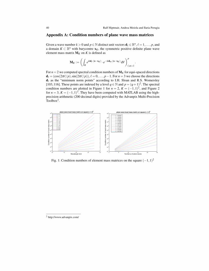
40 Ralf Hiptmair, Andrea Moiola and Ilaria Perugia
Appendix A: Condition numbers of plane wave mass matrices
Given a wave number k > 0 and p∈N distinct unit vectors dℓ ∈Rn, ℓ= 1, . . . , p, and
a domain K ⊂ Rn with barycentre xK , the symmetric positive definite plane wave
element mass matrix MK on K is defined as
MK :=
(∫
Keikdℓ·(x−xK) · e−ikdm·(x−xK) dV
)p
ℓ,m=1
.
For n= 2 we computed spectral condition numbers of MK for equi-spaced directions
dℓ = (cos(2πℓ/p),sin(2πℓ/p)), ℓ= 0, . . . , p−1. For n = 3 we choose the directions
dℓ as the “minimum norm points” according to I.H. Sloan and R.S. Womersley
[103,116]. These points are indexed by a level q ∈N and p = (q+1)2. The spectral
condition numbers are plotted in Figure 1 for n = 2, K = (−1,1)2, and Figure 2
for n = 3, K = (−1,1)3. They have been computed with MATLAB using the high-
precision arithmetic (200 decimal digits) provided by the Advanpix Multi-Precision
Toolbox2.
100
101
102
103
104
100
1010
1020
1030
1040
1050
1060
1070
1080
1090
plane wave local mass matrix on square [−1,1]2
Wavelength 2π/k
Conditio
n n
um
ber
of lo
cal m
ass m
atr
ix
p = 3
p = 5
p = 7
p = 9
p = 11
p = 13
p = 15
p = 17
p = 19
p = 21
p = 23
p = 25
0 5 10 15 20 2510
0
1010
1020
1030
1040
1050
1060
1070
1080
1090
plane wave local mass matrix on square [−1,1]2
Number p of plane waves
Conditio
n n
um
ber
of lo
cal m
ass m
atr
ix
k = 2.000000
k = 1.000000
k = 0.500000
k = 0.250000
k = 0.125000
k = 0.062500
k = 0.031250
k = 0.015625
k = 0.007812
k = 0.003906
k = 0.001953
Fig. 1: Condition numbers of element mass matrices on the square (−1,1)2
2 http://www.advanpix.com/
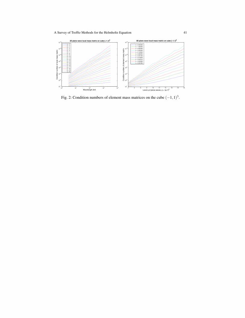
A Survey of Trefftz Methods for the Helmholtz Equation 41
100
101
102
103
104
100
1020
1040
1060
1080
10100
10120
10140
3D plane wave local mass matrix on cube [−1,1]3
Wavelength 2π/k
Co
nd
itio
n n
um
be
r o
f lo
ca
l m
ass m
atr
ix
q = 2
q = 3
q = 4
q = 5
q = 6
q = 7
q = 8
q = 9
q = 10
q = 11
q = 12
q = 13
q = 14
q = 15
q = 16
q = 17
q = 18
q = 19
q = 20
2 4 6 8 10 12 14 16 18 2010
0
1020
1040
1060
1080
10100
10120
10140
3D plane wave local mass matrix on cube [−1,1]3
Level q of plane waves, p = (q+1)2
Co
nd
itio
n n
um
be
r o
f e
lem
en
t m
ass m
atr
ix
k = 2.000000
k = 1.000000
k = 0.500000
k = 0.250000
k = 0.125000
k = 0.062500
k = 0.031250
k = 0.015625
k = 0.007812
k = 0.003906
k = 0.001953
Fig. 2: Condition numbers of element mass matrices on the cube (−1,1)3.

Recent Research Reports
Nr. Authors/Title
2015-10 A. Jentzen and P. PusnikStrong convergence rates for an explicit numerical
approximation method for stochastic evolution equations with
non-globally Lipschitz continuous nonlinearities
2015-11 R. BourquinExhaustive search for higher-order Kronrod-Patterson Extensions
2015-12 R. Bourquin and V. GradinaruNumerical Steepest Descent for Overlap Integrals of Semiclassical Wavepackets
2015-13 A. Hiltebrand and S. MishraEntropy stability and well-balancedness of space-time DG for the shallow waterequations with bottom topography
2015-14 B. Ayuso de Dios and R. Hiptmair and C. PagliantiniAuxiliary Space Preconditioners for SIP-DG Discretizations of H(curl)-ellipticProblems with Discontinuous Coefficients
2015-15 A. Paganini and S. Sargheini and R. Hiptmair and C. HafnerShape Optimization of microlenses
2015-16 V. Kazeev and Ch. SchwabApproximation of Singularities by Quantized-Tensor FEM
2015-17 P. Grohs and Z. KeretaContinuous Parabolic Molecules
Related Documents


![arXiv:1506.04521v2 [math.NA] 4 Sep 2015 · arXiv:1506.04521v2 [math.NA] 4 Sep 2015 A Survey of Trefftz Methods for the Helmholtz Equation Ralf Hiptmair, Andrea Moiola and Ilaria Perugia](https://static.cupdf.com/doc/110x72/5b9bbc1609d3f2d06f8d6295/arxiv150604521v2-mathna-4-sep-2015-arxiv150604521v2-mathna-4-sep-2015.jpg)


