A SURVEY OF COMMODITY MARKETS AND STRUCTURAL MODELS FOR ELECTRICITY PRICES RENE CARMONA AND MICHAEL COULON Abstract. The goal of this survey is to review the major idiosyncrasies of the commodity markets and the methods which have been proposed to handle them in spot and forward price models. We devote special attention to the most idiosyncratic of all: electricity mar- kets. Following a discussion of traded instruments, market features, historical perspectives, recent developments and various modeling approaches, we focus on the important role of other energy prices and fundamental factors in setting the power price. In doing so, we present a detailed analysis of the structural approach for electricity, arguing for its merits over traditional reduced-form models. Building on several recent articles, we advocate a broad and flexible structural framework for spot prices, incorporating demand, capacity and fuel prices in several ways, while calculating closed-form forward prices throughout. 1. Introduction The non-storability of electricity and the wide availability of supply and demand data allow us to understand and analyze the relationship between prices and underlying drivers more easily than in most other markets. These characteristics naturally led to the development of a branch of literature which we refer to as structural models of electricity prices. Making use of similar mathematical tools to the reduced-form models, structural models dig one level deeper, by identifying at least some of the fundamental sources of randomness which appear simply as unobservable diffusion or jump processes in a typical reduced-form approach. In many cases, including such fundamental variables leads to new challenges, due to the very complicated nature of the price setting mechanism in power markets, and difficulty in piec- ing together the key components of the puzzle. Nonetheless, the extra insight on the causes of power price movements brings significant benefits, both in terms of adapting to chang- ing market environments and different locations, as well as in capturing cross-commodity correlations and demand dependence which is crucial for accurate pricing of many common derivatives products and physical assets. Structural models stop short of fully replicating the intricacies of the price setting mechanism (as described by optimization-based stack models) in order to retain tractability and emphasise dominant relationships. Thus, a balance is typ- ically struck between mathematical convenience and model realism. As such, a broad range of structural models exist, which differ both in the number of fundamental relationships they choose to capture and in the techniques used to capture them. Electricity is a commodity and as a result, the electricity markets are most often introduced and studied within the broader framework of the commodity markets. Even though a sig- nificant amount of electricity is generated from renewable sources (e.g. wind and solar) or hydro or nuclear sources, the main production process remains the conversion of fossil fuels like coal, gas and oil. Since electricity is often traded on exchanges just a few hours before it is needed, the overall cost of production is essentially the cost of the fuels used in the production, even in markets with a substantial amount of hydro and nuclear production as these plants are hardly ever setting the price. In other words, since electricity is essentially 2010 Mathematics Subject Classification. Primary 91G20, 91B76. Partially supported by NSF - DMS 0806591. Partially supported by NSF - DMS-0739195. 1

Welcome message from author
This document is posted to help you gain knowledge. Please leave a comment to let me know what you think about it! Share it to your friends and learn new things together.
Transcript
A SURVEY OF COMMODITY MARKETS AND STRUCTURAL MODELS
FOR ELECTRICITY PRICES
RENE CARMONA AND MICHAEL COULON
Abstract. The goal of this survey is to review the major idiosyncrasies of the commoditymarkets and the methods which have been proposed to handle them in spot and forwardprice models. We devote special attention to the most idiosyncratic of all: electricity mar-kets. Following a discussion of traded instruments, market features, historical perspectives,recent developments and various modeling approaches, we focus on the important role ofother energy prices and fundamental factors in setting the power price. In doing so, wepresent a detailed analysis of the structural approach for electricity, arguing for its meritsover traditional reduced-form models. Building on several recent articles, we advocate abroad and flexible structural framework for spot prices, incorporating demand, capacityand fuel prices in several ways, while calculating closed-form forward prices throughout.
1. Introduction
The non-storability of electricity and the wide availability of supply and demand data allowus to understand and analyze the relationship between prices and underlying drivers moreeasily than in most other markets. These characteristics naturally led to the development ofa branch of literature which we refer to as structural models of electricity prices. Making useof similar mathematical tools to the reduced-form models, structural models dig one leveldeeper, by identifying at least some of the fundamental sources of randomness which appearsimply as unobservable diffusion or jump processes in a typical reduced-form approach. Inmany cases, including such fundamental variables leads to new challenges, due to the verycomplicated nature of the price setting mechanism in power markets, and difficulty in piec-ing together the key components of the puzzle. Nonetheless, the extra insight on the causesof power price movements brings significant benefits, both in terms of adapting to chang-ing market environments and different locations, as well as in capturing cross-commoditycorrelations and demand dependence which is crucial for accurate pricing of many commonderivatives products and physical assets. Structural models stop short of fully replicating theintricacies of the price setting mechanism (as described by optimization-based stack models)in order to retain tractability and emphasise dominant relationships. Thus, a balance is typ-ically struck between mathematical convenience and model realism. As such, a broad rangeof structural models exist, which differ both in the number of fundamental relationships theychoose to capture and in the techniques used to capture them.
Electricity is a commodity and as a result, the electricity markets are most often introducedand studied within the broader framework of the commodity markets. Even though a sig-nificant amount of electricity is generated from renewable sources (e.g. wind and solar) orhydro or nuclear sources, the main production process remains the conversion of fossil fuelslike coal, gas and oil. Since electricity is often traded on exchanges just a few hours beforeit is needed, the overall cost of production is essentially the cost of the fuels used in theproduction, even in markets with a substantial amount of hydro and nuclear production asthese plants are hardly ever setting the price. In other words, since electricity is essentially
2010 Mathematics Subject Classification. Primary 91G20, 91B76.Partially supported by NSF - DMS 0806591.Partially supported by NSF - DMS-0739195.
1
2 RENE CARMONA AND MICHAEL COULON
not storable, it must be consumed as it is produced and the costs of production are animportant part of the computation of the supply curve. For this reason, electricity priceformation cannot be dissociated from the prices of the fuels used in its production.
In this context, it is clear that valuation should be done by equilibrium arguments matchingsupply and demand. This paper reviews some of the mathematical models used by academicsand practitioners alike, and provides an introduction to the class of structural models whichbuild on this idea. The present introduction gives a series of anecdotes illustrating therecurrent themes developed in the paper.
Electricity burst onto the financial scene with deregulation and the transition from a systemwhere production, transportation, and distribution of electricity were vertically integratedunder the monopoly of utilities, to a set of open competitive markets for production andretail, while the grid remained under control. This unbundling happened over a few yearsin several parts of the world, but was not equally successful. NordPool (Northern Europe),ERCOT (Texas), PJM (North East of the US) are generally regarded as successes but theCalifornia experience of the early 2000’s was controversial and most of its original initiativesended up being reversed in the long run. In any case, deregulation opened up new marketsand a new price formation mechanism emerged based on constant supply - demand balance.While electricity shares equilibrium pricing with most other commodities, it stands out bythe construction of the supply curve where the different modes of production (hydro, nuclear,solar, wind, coal, oil, gas, etc) are ordered (the resulting order being called merit order) inincreasing order of costs of production, resulting in what is known as the production stack.Matching supply with demand leads to the concept of plant on the margin (or technologyon the margin) which is fundamental in the understanding of price formation for electricity,and which is at the heart of the approach taken in this presentation.
The business of producing, delivering and retailing electricity is very complex. It requirescapital intensive investments and long term financing. Financial mathematics and financialengineering have an important role to play, far beyond the traditional support of portfoliomanagement. The first challenge has to do with a very different breed of data analysis: costsand prices are not always available, and when they are, the amount and the complexity of thedata can be overwhelming. The multitude of locations (e.g. nodal pricing), the diverse natureof the electricity contracted (spot, day-ahead, on-peak, off-peak, firm, non-firm, forward,. . .),and the fact that, contrary to other commodities and financial products, electricity prices canbe negative. And as if the challenges of the analysis of electricity price data was not enough,quants have to deal with a slew of derivative products with embedded features rarely seen onthe traditional financial markets. They include features known as swings, recall / take-or-payoptions, etc, and new derivatives intended to help market participants hedge some of the risksassociated with physical factors impacting the bottom line (weather and emissions, tollingagreements, shipping and freight, gas storage, cross commodity derivatives, etc). Whilebeing a constant nightmare for regulators and managers, the complexity and the diversityof these derivatives became a bonanza for financial engineers and financial mathematicianswho discovered a brand new source of challenging modeling and pricing problems. See forexample [57, 32, 23] and the more recent articles [80, 14, 75] for a sample of mathematicaland numerical developments prompted by the analysis of swing options.
Finally, the need to quantify the credit-worthiness of counter-parties and integrate this in-formation in the valuation algorithms, became painfully obvious after the collapse of Enronand the ensuing rash of defaults in the industry. Ironically, Enron was one of the very firstcompanies advocating the need to take counterparty credit-worthiness into account in anyvaluation exercise. The avalanche of bankruptcies and credit downgrades following Enron’scollapse highlighted the need for a deep understanding of the statistics of credit migration,appropriate ways to include counter-party risk in the valuation of transactions, and possiblythe enhancement of credit protection with specific derivative instruments. Unfortunately,
COMMODITIES AND ELECTRICITY MODELING 3
many of these derivatives depend upon industry indexes based on actual movements in themarkets and these indexes have been proven to be easy targets of manipulation. Systematicreliance on clearing houses has been proposed as the ultimate solution to these uncertainties,and living with collateral requirements and margin calls is part of the every-day life of anenergy trader. However, most transactions rely on tailor-made deals and it seems difficult toimagine that a minimal set of instruments could be designed in order to span all the energycontracts and make clearing a standard solution. We will not discuss these problems in thissurvey any further.
Under the influence of Enron, quants and academics alike embraced the real option approachto physical asset valuation, providing systematic ways to include the physical assets of a com-pany (power plants, pipelines, barges, tankers, etc.) together with the financial instrumentsheld at a given time, into a single portfolio. This innovative way to put together apples andoranges on the same book, opened the door to new forms of hedging the risks of financialpositions using physical assets, or vice-versa. Undoubtedly, one of the most exciting chal-lenges of the energy markets is the new breed of hedging imposed by the physical nature ofthe commodities underlying the financial contracts, and risk management of production andtransportation facilities. Indeed, hedging the risks associated with mixtures of physical andfinancial assets is not part of the typical financial mathematics curriculum. While a necessityfor electricity producers and retailers, it was perfected and developed into an art form byinvestment banks like Goldman Sachs, Morgan Stanley, JP Morgan and the like, which inorder to optimize returns, have sited and leased power plants, and taken control of storagefacilities and the transportation of goods via leasing of pipelines, tankers, etc. More than adecade later, these problems are still important drivers in academic research in commodityand energy market modeling, and the constant flow of academic publications on power plantand gas storage facility valuations is a case in point. While no obvious benchmark emerged,some of these methods are widely accepted and their use for marking to market purposes hasbecome a common practice accepted by regulators. However, the physical nature of some ofthe assets in the portfolios of energy companies renders the computation of correlations andrisk measures like Value at Risk (VaR) very much a challenge.
The simplest form of real option valuation of a power plant is to equate its value to a string ofspread options, each option capturing the potential profit from the operation of the plant ona given day. In a nutshell this approach says that on any given day, if the difference betweenthe price at which the electricity can be sold and the cost of the input fuels needed to produceit (plus the fixed costs of operation and maintenance of the plant) is positive, the plant shouldbe run and this difference collected as a profit. While commonly relying on simple lognormalmodels for the prices of electricity and the input fuels (see for example [49, 25]), any pricingmodel with a new approach to capturing the dependence between electricity prices and theprices of the input fuels is likely to produce new plant valuation results. In this spirit, [31]suggests models integrating information about correlation contained in the prices of spreadoptions traded on the market in the form of implied correlations. In this survey, we willreview how the structural approach developed in [21] can provide valuations depending onfuture demand expectations and information contained in the forward curves of the inputfuels. Viewing a power plant as a string of spread options is certainly not the only way tovalue power plants. More sophisticated methods use stochastic control techniques to takefull advantage of the optionality of the plant. See for example [30, 3]. Moreover, some ofthese methods have been extended to value gas storage and we refer the interested reader to[28, 27, 50, 77]. and the references therein. However, as demonstrated in [21], the structuralapproach focuses more on energy price correlations and offers the flexibility of adapting tofuture scenarios for demand, capacity and input fuel forward prices.
The versatility and the adaptability of the structural approach is the main reason for ourshameless attempt to promote it. As discussed further in Subsection 2, the commodity
4 RENE CARMONA AND MICHAEL COULON
and energy markets have seen dramatic changes in the last few years. The impact of someof these changes on electricity prices is rather subtle and cannot be easily captured bytraditional reduced form models. The introduction of incentive programs favoring the useof renewable energy such as wind in Germany or solar in the US, the impact of mandatoryregulations such as the European Union (EU) Emissions Trading Scheme (ETS) in Europe,the recent physical coupling of markets (e.g. France and Germany), the increase in correlationbetween stock and commodity prices due to index trading, the tightening of correlationsbetween commodities included in these indexes, the dramatic drop in US natural gas pricesfollowing recent shale gas discoveries and large-scale development of fracking, etc. All ofthese changes are screaming for the use of flexible models which can accommodate these newrelationships between the fundamental factors driving electricity prices. Historical pricesmay not be as relevant as forward-looking information and market knowledge: this givesstructural approaches a big advantage over reduced-form models.
Excellent textbooks on mathematical models for the electricity (and other commodity) mar-kets do exist, and we strongly recommend the reader to consult [13, 18, 38, 49, 52, 53, 67, 78]for the many aspects of the markets which we will not be able to cover in this survey.
We close this introduction with an outline of the contents of the paper. Section 2 givesa crash course on the commodity markets. The focus is mostly on energy and trading ofthe fuels entering the production of electricity. A discussion of the impact of index tradingis included to emphasize, for better or worse, the growing socio-economic role played bycommodity trading. The specific nature of the data needed to understand these markets isdiscussed and the importance of the forward markets is reflected in the construction of pricemodels. The goal of Section 3 is to highlight how different electricity is from the other energycommodities. Its non-storability forces a difficult balancing act where supply and demandneed to be matched in real time since electricity needs to be consumed as it is produced.Section 4 expands on the earlier discussions to introduce the building blocks of the structuralmodels which we advocate in this survey. Section 5 then uses these ingredients to proposegeneral classes of structural models for which closed-form prices of forward contracts canbe found. We also discuss various issues related to model fitting and calibration, beforeconcluding in Section 6.
2. Generalities on the Commodity Markets
As explained in the introduction, in order to understand the fundamentals of electricityprices, and especially the rationale for the structural models which we advocate, it is impor-tant to understand how electricity is produced, and the costs associated to the various fuelsused in the process. This is the main reason for the need to understand the crude oil, coaland natural gas markets (before returning to electricity in the next section). Despite thefact that these represent only a small part of the commodity world, we discuss their mainfeatures as they pertain to commodity markets in general.
2.1. Trading Commodities. Commodities are considered as a separate asset class. Be-cause of the physical nature of the interest underlying the contracts, their prices are deter-mined by equilibrium arguments which involve matching supply and demand for the physicalcommodity itself. On the supply side, estimating and predicting inventories and quantifyingthe costs of storage and delivery are important factors which need to be taken into account.This is not always easy in the context of standard valuation methods which are mostly basedon traditional finance theory (think for example of NPV which attempts to compute thepresent value of the flow of future dividends).
Whether they were called spot markets (when they involved the immediate delivery of thephysical commodity), or forward markets (when delivery was scheduled at a later date),
COMMODITIES AND ELECTRICITY MODELING 5
commodity markets started as physical markets. Trading volume exploded with the appear-ance of financially settled contracts. While forward contracts are settled Over the Counter(OTC), and as such, carry the risk that the counterparty may default and not meet theterms of the contract, most of the financially settled contracts are exchange-traded futuresfor which the exchange acts as clearing house controlling default risk by a system of mar-gin calls and attracting speculators to provide liquidity to the markets. While trading inphysically and financially settled contracts were traditionally the two ways an investor couldgain exposure to commodities, the creation of indexes and the increasing popularity of in-dex tracking Exchange Traded Funds (ETFs) have offered a new way to gain exposure tocommodities. Investing in commodities was promoted as the perfect portfolio diversificationtool as they were believed to be negatively correlated with stocks. The exponential growth ofthis new form of investment in commodities which took place over the last decade may havebeen a self-defeating prophecy as recent econometric studies have shown that this form ofindex trading has created new correlations between commodities and stocks, and betweenthe commodities included in the same index. Furthermore, Bouchouev [17] argues that theinfluence of investors has overturned Keynes’ well-known ‘theory of normal backwardation’,causing a recent predominance of forward curves in contango, thus further weakening theattractiveness of investing in these markets.
One of the many convenient features of commodity trading is the specialization of the ex-changes, leading to a simple correspondence between commodities and locations where theyare traded. In other words, a given commodity is traded on one or a small number of spe-cialized exchanges. The following table gives a few examples of some of these exchanges inthe US and in Europe.
Exchange Location Contracts
Chicago Board of Trade (CBOT) Chicago Grains, Ethanol, MetalsChicago Mercantile Exch. (CME) Chicago, US Meats, Currencies, EurodollarsIntercontinental Exch. (ICE) Atlanta, US Energy, Emissions, AgriculturalKansas City Board of Trade (KCBT) Kansas City, US AgriculturalNew York Merc. Exch. (NYMEX) New York, US Energy, Prec. Metals, Indust. MetalsClimex (CLIMEX) Amsterdam, NL. EmissionsNYSE Liffe Europe AgriculturalEuropean Climate Exch. (ECX) Europe EmissionsLondon Metal Exch. (LME) London, UK Industrial Metals, Plastics
There are several ways in which investors gain exposure to commodities.
1. The old fashion way to invest in commodities is to actually purchase the physical com-modity itself. However most investors are not ready or equipped to deal with issues oftransportation, delivery, storage and perishability. This form of involvement in commoditieswas created for and is essentially limited to the naturals, namely the hedgers who mitigatethe financial risks associated with uncertainties in their production and delivery of thesecommodities.
2. Another way to gain exposure to commodities is to invest in stocks in commodity intensivebusinesses: for example buying shares of Exxon or Shell as a way to invest in oil. However,this type of investment offers at best an indirect exposure as shares of natural resourcecompanies are not perfectly correlated with commodity prices.
3. A more direct form is straight investment in commodity futures and options. The ex-changes offer transparency and integrity through clearing and relatively small initial invest-ments are needed to take large positions through leverage. However, this convenience comesat a serious price as discovered by many rookies who ended up choking, unable to face the
6 RENE CARMONA AND MICHAEL COULON
margin calls triggered by adverse moves of the values of the interests underlying the futurescontracts. Also, purely speculative investments of this type may need to be structured witha careful rolling forward of the contracts approaching maturity in order to avoid having totake physical delivery of the commodity: trading wheat futures can be done from the comfortof an office set up in a basement, but taking physical delivery of one lot (i.e. 5, 000 bushels)of wheat requires a large backyard!
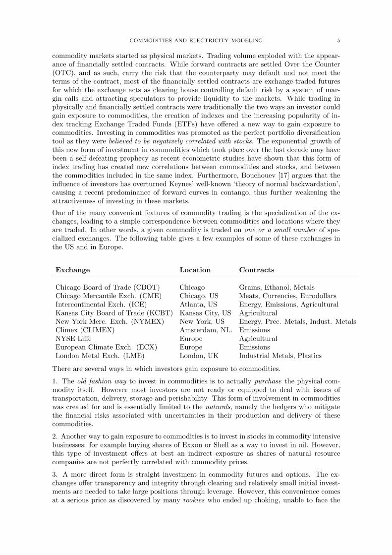
4. The final way to gain exposure to commodity which we discuss is investing directly inCommodity Indexes or in Exchange Traded Funds (ETFs) tracking these commodity indexes.Many ETFs simply invest in the nearest forward contract and automatically ‘roll’ the in-vestment into the next month’s contract near maturity. This form of passive investment(after all there is no need for a Commodity Trading Advisor (CTA) for that), has becomevery popular as a way to diversify an investment portfolio with an exposure to commoditieswithout having to deal with the gory details of all the convoluted idiosyncrasies of the rel-evant markets. Nevertheless, an understanding of forward curve dynamics and the effect ofmonthly rolls is still vital, as a recent investor in the natural gas ETF would undoubtedlyagree: between June 2008 and March 2012 this ETF (called UNG) lost a shocking 96% of itsvalue, with roughly half attributable to the spot price drop and half to the steep contangowitnessed throughout this period.
-0.2
0.00.2
0.40.6
1995 2000 2005 2010
Time Series Plot of BETA.ts
Figure 1. Instantaneous Dependence (β) of GSCI-TR returns upon S&P 500 returns.
According to Barclays’ internal reports, in 2006 - 2007, index fund investment increased from90 billion to 200 billion USD. Simultaneously, commodity prices increased 71% as measuredby the CRB index. However, when prices declined dramatically from June 2008 throughearly 2009, many pointed to the large scale speculative buying by index funds, arguing thatthis created a bubble as futures prices far exceeded fundamental values. Some economists(including Nobel Prize winner P. Krugman, Pirrong, Sanders, Irwin, Hamilton and Kilian)remained skeptic about the “bubble theory” arguing that prices of commodities are set bysupply and demand, and that rapid growth in emerging economies (e.g. China) increaseddemand and caused the 2008 surge in price. This did not stop commodity index investingfrom being under attack. Increased participation in futures markets by non-traditional in-vestors was deemed disruptive and blamed for the 2007-2008 “Food Crisis” that is at theorigin of the famous “Casino of Hunger: How Wall Street Speculators Fueled the GlobalFood Crisis”. A report from the U.S. Senate Permanent Subcommittee on Investigation“... finds that there is significant and persuasive evidence to conclude that these commodityindex traders, in the aggregate, were one of the major causes of unwarranted increases in the
COMMODITIES AND ELECTRICITY MODELING 7
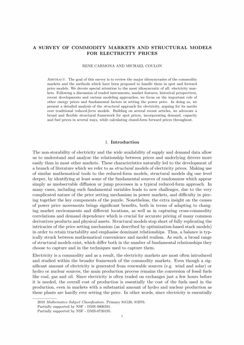
price of wheat futures contracts relative to the price of wheat in the cash market.....” . Toadd insult to injury, a group of 48 agriculture ministers meeting in Berlin said they were “...concerned that excessive price volatility and speculation on international agricultural marketsmight constitute a threat to food security....”, according to a joint statement handed out toreporters on Jan. 22, 2011. It is an empirical fact that return correlations are no longerwhat they used to be and now commonly accepted that commodity index trading tightenedcorrelations between commodities [73]. However, many argue that this is a scale dependentphenomenon and it seems that high frequency traders do not see (and hence ignore) thesecorrelation increases. Broadly speaking, the financialization of commodities should refer tothe increased leverage and the exponential growth of financially settled contracts dwarfingtheir physically settled counterparts. More recently, this term has been used to refer to thesignificant impact of index trading on commodity prices, and even more narrowly speaking,to the increased correlations between the commodities included in the same index and alsobetween equity returns and commodity index returns. This last fact is illustrated in Figure1 which shows the time evolution as given by a Kalman filter, of the time-dependent “beta”of the least squares linear regression of the Goldman Sachs Commodity Index Total Returnagainst the returns of the S&P 500 index.
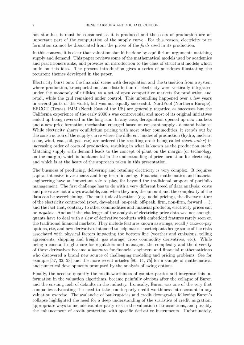
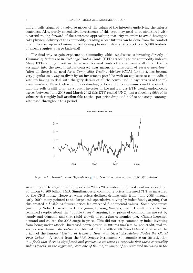
In this paper, our interest in commodities is mostly focused on the commodities used in theproduction of electricity, and in particular to crude oil and natural gas which are heavilyrepresented in most commodity indexes. What we learn from the above discussion is thatrecent changes may affect their correlation and the correlation they have with the broaderfinancial markets. Figure 2 shows weekly average spot (or nearest forward) prices for elec-tricity, natural gas and crude oil, and illustrates the strong correlations between these energycommodities over a ten-year period. While the 2008 ‘bubble’ is most dramatic for crude oil,natural gas and power prices also rose sharply. In our search for electricity pricing models, itis important to bear in mind the diverse and changing factors affecting commodity marketsin general.
!"
#!"
$!"
%!"
&!"
'!!"
'#!"
'$!"
'%!"
()*+!!
"
()*+!'
"
()*+!#
"
()*+!,
"
()*+!$
"
()*+!-
"
()*+!%
"
()*+!.
"
()*+!&
"
()*+!/
"
()*+'!
"
0(1"23456"789":;<=>"?@A"B@C":D'!>"
Figure 2. Weekly average prices for PJM (US electricity), Henry Hub (US naturalgas) and WTI (US crude oil). Natural gas is multiplied by 10 to use the same axis.
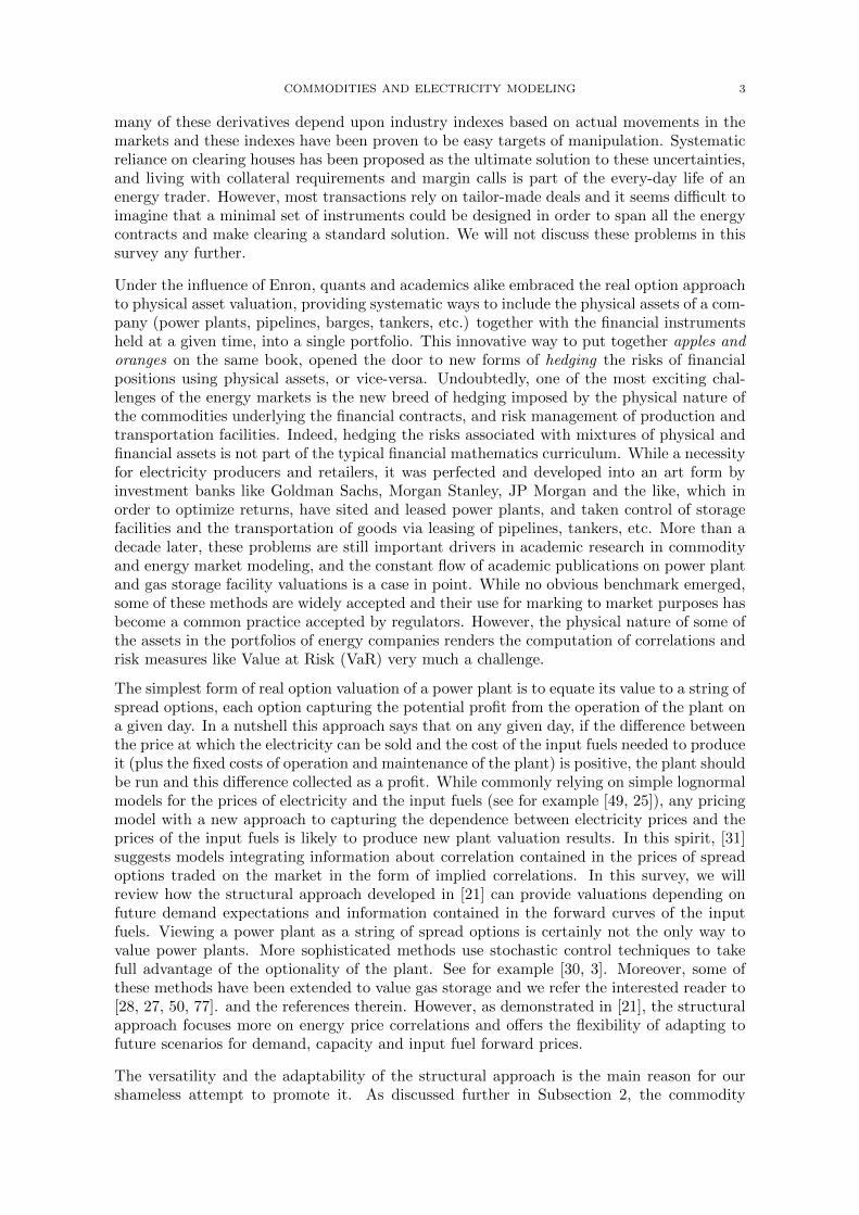
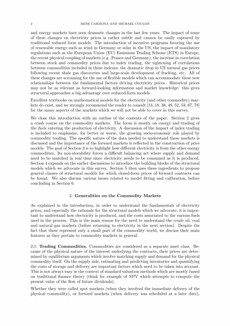
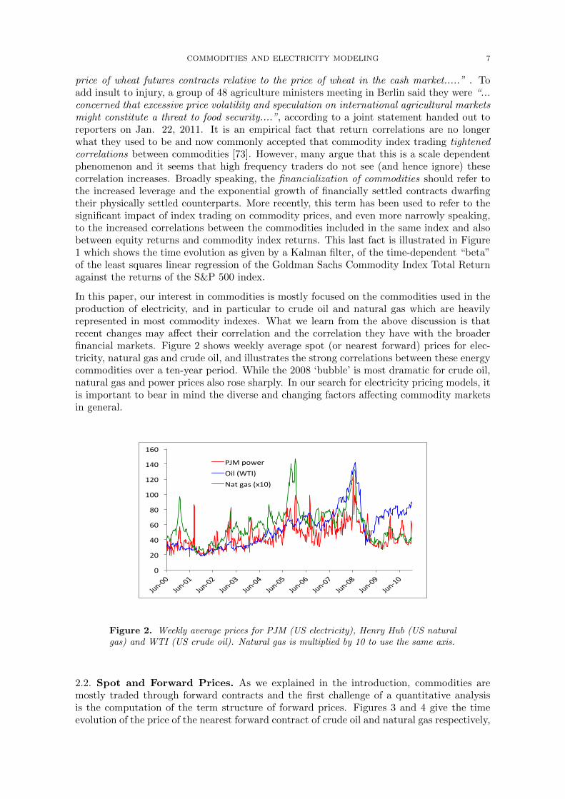
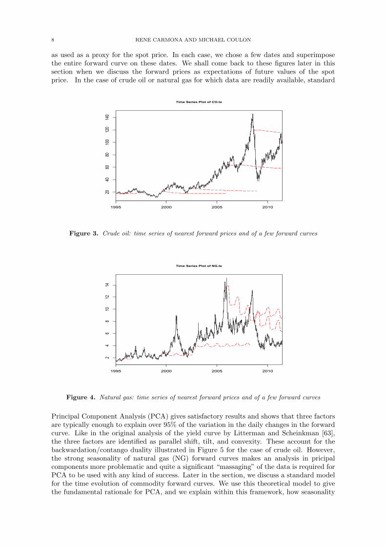
2.2. Spot and Forward Prices. As we explained in the introduction, commodities aremostly traded through forward contracts and the first challenge of a quantitative analysisis the computation of the term structure of forward prices. Figures 3 and 4 give the timeevolution of the price of the nearest forward contract of crude oil and natural gas respectively,
8 RENE CARMONA AND MICHAEL COULON
as used as a proxy for the spot price. In each case, we chose a few dates and superimposethe entire forward curve on these dates. We shall come back to these figures later in thissection when we discuss the forward prices as expectations of future values of the spotprice. In the case of crude oil or natural gas for which data are readily available, standard
2040
6080
100
120
140
1995 2000 2005 2010
Time Series Plot of CO.ts
Figure 3. Crude oil: time series of nearest forward prices and of a few forward curves
24
68
1012
14
1995 2000 2005 2010
Time Series Plot of NG.ts
Figure 4. Natural gas: time series of nearest forward prices and of a few forward curves
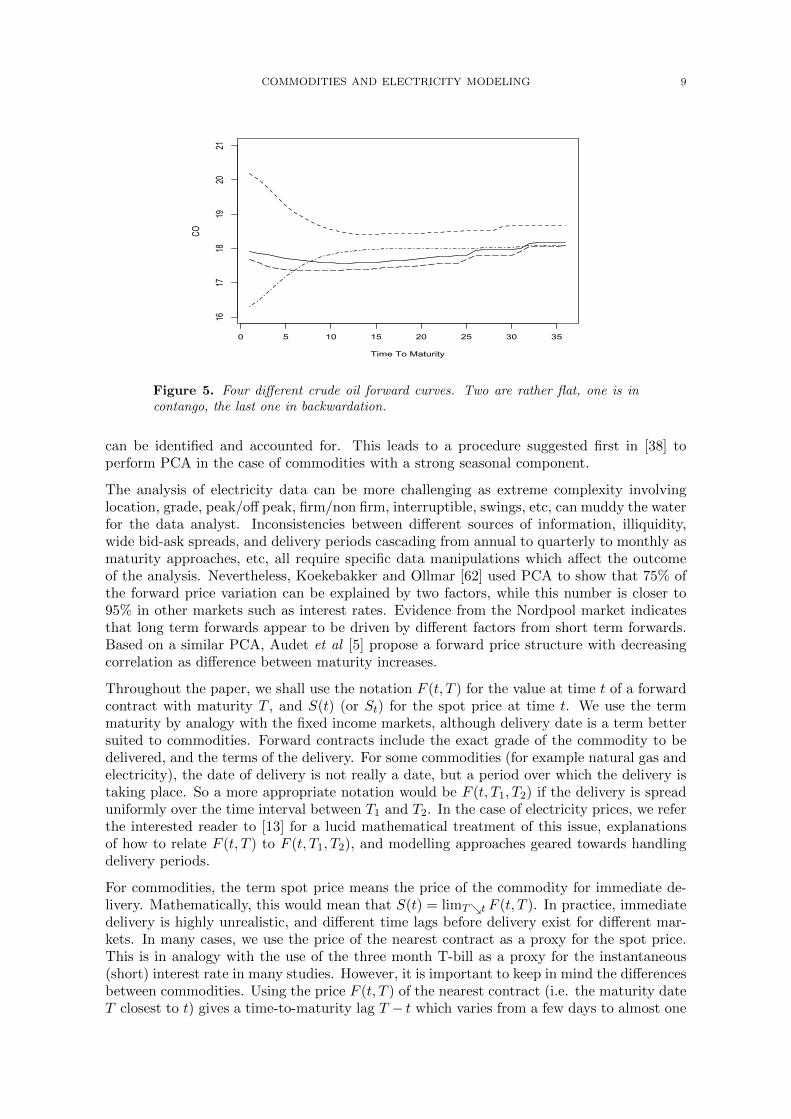
Principal Component Analysis (PCA) gives satisfactory results and shows that three factorsare typically enough to explain over 95% of the variation in the daily changes in the forwardcurve. Like in the original analysis of the yield curve by Litterman and Scheinkman [63],the three factors are identified as parallel shift, tilt, and convexity. These account for thebackwardation/contango duality illustrated in Figure 5 for the case of crude oil. However,the strong seasonality of natural gas (NG) forward curves makes an analysis in pricipalcomponents more problematic and quite a significant “massaging” of the data is required forPCA to be used with any kind of success. Later in the section, we discuss a standard modelfor the time evolution of commodity forward curves. We use this theoretical model to givethe fundamental rationale for PCA, and we explain within this framework, how seasonality
COMMODITIES AND ELECTRICITY MODELING 9
0 5 10 15 20 25 30 35
1617
1819
2021
Time To Maturity
CO
Figure 5. Four different crude oil forward curves. Two are rather flat, one is incontango, the last one in backwardation.
can be identified and accounted for. This leads to a procedure suggested first in [38] toperform PCA in the case of commodities with a strong seasonal component.
The analysis of electricity data can be more challenging as extreme complexity involvinglocation, grade, peak/off peak, firm/non firm, interruptible, swings, etc, can muddy the waterfor the data analyst. Inconsistencies between different sources of information, illiquidity,wide bid-ask spreads, and delivery periods cascading from annual to quarterly to monthly asmaturity approaches, etc, all require specific data manipulations which affect the outcomeof the analysis. Nevertheless, Koekebakker and Ollmar [62] used PCA to show that 75% ofthe forward price variation can be explained by two factors, while this number is closer to95% in other markets such as interest rates. Evidence from the Nordpool market indicatesthat long term forwards appear to be driven by different factors from short term forwards.Based on a similar PCA, Audet et al [5] propose a forward price structure with decreasingcorrelation as difference between maturity increases.
Throughout the paper, we shall use the notation F (t, T ) for the value at time t of a forwardcontract with maturity T , and S(t) (or St) for the spot price at time t. We use the termmaturity by analogy with the fixed income markets, although delivery date is a term bettersuited to commodities. Forward contracts include the exact grade of the commodity to bedelivered, and the terms of the delivery. For some commodities (for example natural gas andelectricity), the date of delivery is not really a date, but a period over which the delivery istaking place. So a more appropriate notation would be F (t, T1, T2) if the delivery is spreaduniformly over the time interval between T1 and T2. In the case of electricity prices, we referthe interested reader to [13] for a lucid mathematical treatment of this issue, explanationsof how to relate F (t, T ) to F (t, T1, T2), and modelling approaches geared towards handlingdelivery periods.
For commodities, the term spot price means the price of the commodity for immediate de-livery. Mathematically, this would mean that S(t) = limT↘t F (t, T ). In practice, immediatedelivery is highly unrealistic, and different time lags before delivery exist for different mar-kets. In many cases, we use the price of the nearest contract as a proxy for the spot price.This is in analogy with the use of the three month T-bill as a proxy for the instantaneous(short) interest rate in many studies. However, it is important to keep in mind the differencesbetween commodities. Using the price F (t, T ) of the nearest contract (i.e. the maturity dateT closest to t) gives a time-to-maturity lag T − t which varies from a few days to almost one
10 RENE CARMONA AND MICHAEL COULON
month as t varies. So when we use such a proxy for the spot price of crude oil or natural gas,the resulting approximation evolves over time as an accordion. However, when treating theprice for next day delivery as the spot price of electricity, this phenomenon is not presentsince T − t remains constant and equal to one day!
One of the most useful concepts for the analysis of instruments traded on a forward basis isthe Spot - Forward relationship which was proven to be a powerful tool in the analysis offinancial markets where one can hold positions at no cost and easily take short positions. Inthat case, a simple arbitrage argument shows that
F (t, T ) = S(t)er(T−t),
where r denotes the short interest rate. Since we are using a deterministic interest rate,forward and futures prices coincide in our mathematical treatment. Furthermore
F (t, T ) = Et[S(T )]
where the above expectation is a risk neutral expectation conditioned by all the informa-tion available at time t. However, when bought with the intent to be sold later, a physicalcommodity needs to be transported and stored, adding to the cost of the financing of thepurchase. On the other hand, holding the physical commodity can be advantageous, particu-larly in times of market stress or during supply shocks. The theory of storage was developedwith the intention of explaining normal backwardation arguing that F (t, T ) is a downwardbiased estimate of S(T ), namely the spot price exceeds the forward prices. (See Figures 3and 4 for examples.) In order to translate this into a reduced-form expression and explain thedifferent relationships between spot and forward prices, the notion of convenience yield wasintroduced. Next we review some of the quirks of this theory, even though we should keepin mind that while it can be applied to crude oil, natural gas, coal (fuels used in electricityproduction), it does not apply to electricity prices since for all practical purposes, electricityis not a storable commodity.
The Case of Storable Commodities. The argument above leads to the formula
F (t, T ) = S(t)e(r−δ)(T−t)
for some quantity δ ≥ 0 which is called the convenience yield. If we decompose this quantityin the form δ = δ1 − c with δ1 modeling the benefit from owning the physical commodityand c the costs of storage, then
F (t, T ) = er(T−t)e−δ1(T−t)e−c(T−t)
where er(T−t) represents the cost of financing the purchase, ec(T−t) the cost of storage, ande−δ1(T−t) the sheer benefit from owning the physical commodity. The advantage of thisrepresentation, as artificial as it may be, is to explain the backwardation / contango dualitywithin the proposed framework. Indeed, backwardation which occurs when the curve T ↪→F (t, T ) = S(t)e(r+c−δ1)(T−t) is decreasing holds when r + c < δ1, namely when benefitsof holding the commodity outweigh interest rates and storage costs. On the other hand,the forward curve is in contango, namely the curve T ↪→ F (t, T ) = S(t)e(r+c−δ1)(T−t) isincreasing, when r + c ≥ δ1. Empirical evidence shows that the convenience yield changesover time, and that it is related to several economic indicators, and in particular, inverselyrelated to inventory levels. So it is natural, as we do next, to include it as a stochastic factorin a pricing model.
2.3. Convenience Yield Models. For quite a long time, the standard model has been theGibson-Schwartz [55] two-factor model with factors given by the commodity spot price Stand the convenience yield δt. It posits risk neutral dynamics of the form
(1)
{dSt = (rt − δt)St dt+ σSt dW
1t ,
dδt = κ(θ − δt)dt+ σδ dW2t .
COMMODITIES AND ELECTRICITY MODELING 11
One of the major attraction of the model is that, being a particular case of the so-calledexponential affine models, explicit formulas are available for many derivatives. In particularthe prices of the forward contracts are given by
F (t, T ) = Ste∫ Tt rsdseB(t,T )δt+A(t,T )
where
B(t, T ) =e−κ(T−t) − 1
κ,
A(t, T ) =κθ + ρσsγ
κ2(1− e−κ(T−t) − κ(T − t)) +
+γ2
κ3(2κ(T − t)− 3 + 4e−κ(T−t) − e−2κ(T−t)).
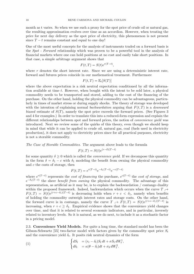
However, as demonstrated in [29], this strength of the model comes at a price. For any givenmaturity T , one can follow the time evolution of the forward price F (t, T ) from market quotes,and from the above formulae, one can infer for each day t, the value of the convenience yield δt.Internal consistency of the model requires that this implied convenience yield is independentof the choice of the particular contract maturity T . However, Figure 6 borrowed from [29]shows that this is not the case. Instabilities and inconsistencies in the implied δt demonstratethat the two factor model ignores significant maturity specific effects.
Figure 6. Crude oil convenience yield implied by a 3 month futures contract (left);Difference in implied convenience yields between 3 and 12 month contracts. (right)
As suggested in [29], one possible way out of this quandary is to model directly the historicaldynamics, for each fixed maturity T0, of the forward price Ft = F (t, T0) instead of the spotSt, assuming that
dFt = (µt − δt)Ft dt+ σFt dW1t ,
dδt = κ(θ − δt)dt+ σδ dW2t
or more generallydδt = b(δt, Ft)dt+ σδ(δt, Ft)dW
2t .
One can still compute the values of the convenience yield implied by the model. Indeed theassumption that Ft is tradable and observable while the forward convenience yield δt is not,sets up a standard filtering problem which can be solved to construct a convenience yield
12 RENE CARMONA AND MICHAEL COULON
for each maturity. See [29] for details. There are other approaches to modeling the termstructure of convenience yield, and the reader may want to consult [15] for a risk neutralapproach a la Heath-Jarrow-Morton (HJM) which bares to the Gibson-Schwartz model (1)the same relationship as the classical HJM models to the standard short rate models.
2.4. Dynamic Model for the Forward Curves. In this subsection, we follow [38] todescribe a standard HJM-like n-factor forward curve model which we use to derive thedynamics of the spot commodity model, and prepare for the explanations given in the nextsubsection on how to calibrate the model to price data using PCA, even when strong seasonaleffects spoil a direct and naive application of the method. We start with a model under thehistorical measure
(2)dF (t, T )
F (t, T )= µ(t, T )dt+
n∑k=1
σk(t, T )dWk(t) t ≤ T
where W = (W1, . . . ,Wn) is a n-dimensional standard Brownian motion, and the drift µ andthe volatilities σk are deterministic functions of t and the time-of-maturity T . Notice thatµ(t, T ) will be set to zero for pricing purposes. In general, µ(t, T ) is calibrated to historicaldata for risk management applications. By the simplicity of this lognormal model, explicitsolutions exist for the forward prices:
F (t, T ) = F (0, T ) exp
[∫ t
0
[µ(s, T )− 1
2
n∑k=1
σk(s, T )2
]ds+
n∑k=1
∫ t
0σk(s, T )dWk(s)
]and the forward prices are log-normal random variables of the form
F (t, T ) = αeβX−β2/2
with X ∼ N(0, 1) and
α = F (0, T ) exp
[∫ t
0µ(s, T )ds
], and β =
√√√√ n∑k=1
∫ t
0σk(s, T )2ds
From these, we can derive an expression for the spot price S(t) = F (t, t) defined as the lefthand point of the forward curve:
S(t) = F (0, t) exp
[∫ t
0[µ(s, t)− 1
2
n∑k=1
σk(s, t)2]ds+
n∑k=1
∫ t
0σk(s, t)dWk(s)
]and differentiating both sides we get an equation for its dynamics:
dS(t) = S(t)
[(1
F (0, t)
∂F (0, t)
∂t+ µ(t, t) +
∫ t
0
∂µ(s, t)
∂tds− 1
2σS(t)2
−n∑k=1
∫ t
0σk(s, t)
∂σk(s, t)
∂tds+
n∑k=1
∫ t
0
∂σk(s, t)
∂tdWk(s)
)dt+
n∑k=1
σk(t, t)dWk(t)
]from which we can identify the spot volatility
(3) σS(t)2 =
n∑k=1
σk(t, t)2.
Hence, if we define the Wiener process Wt by Wt = σS(t)−1∑n
k=1 σk(t, t)dWk(t), then thedynamics of the spot can be rewritten in the form:
dS(t)
S(t)=
[∂ logF (0, t)
∂t+ d(t)
]dt+ σS(t)dWt
COMMODITIES AND ELECTRICITY MODELING 13
provided we define the drift component d(t) by:
d(t) = µ(t, t)− 1
2σS(t)2 +
∫ t
0
∂µ(s, t)
∂tds−
n∑k=1
∫ t
0σk(s, t)
∂σk(s, t)
∂tds
+
n∑k=1
∫ t
0
∂σk(s, t)
∂tdWk(s).
Looking more closely at the expression giving the drift we notice that, in a risk-neutralsetting, the logarithmic derivative of the forward can be interpreted as a discount rate, whiled(t) can be interpreted as a convenience yield. We also notice that the drift is generallynot Markovian. However, in the particular case of a single factor, when µ(t, T ) ≡ 0, and
σS(t) = σ1(t, T ) = σe−λ(T−t) which is consistent with what is known as the Samuelson’seffect, we have
d(t) = λ[logF (0, t)− logS(t)] +σ2
4λ(1− e−2λt),
and the dynamics of the spot become
dS(t)
S(t)= [µ(t)− λ logS(t)]dt+ σdW (t),
which shows that in this case, the spot price is an exponential Ornstein Uhlenbeck process,an instance of the formal equivalence between mean reversion and the exponential decay ofthe forward volatility away from maturity.
2.5. Rationale for PCA. For data analysis and computational purposes, it is convenientto change variable from the time-of-maturity T to the time-to-maturity τ . This changes thedependence upon t in several formulae. To be specific, if we set
t ↪→ F (t, T ) = F (t, t+ τ) = F (t, τ)
for pricing purposes, it is important to keep in mind that for T fixed, {F (t, T )}0≤t≤T is a
martingale while for τ fixed, {F (t, τ)}0≤t is NOT ! The dynamics of the forward prices inthis parameterization (known as Musiela parameterization) become
dF (t, τ) = F (t, τ)
[(µ(t, τ) +
∂
∂τlog F (t, τ)
)dt+
n∑k=1
σk(t, τ)dWk(t)
], τ ≥ 0
if we set:
µ(t, τ) = µ(t, t+ τ), and σk(t, τ) = σk(t, t+ τ).
We use the above model for the evolution of the forward curves to justify PCA, and in sodoing, we explain how to handle seasonal effects (as seen in the case of natural gas). Ourfundamental assumption is that the volatilities appearing in (2) are of the form
σk(t, T ) = σ(t)σk(T − t) = σ(t)σk(τ)
for some function t ↪→ σ(t). Then, the spot volatility σS(t) defined in (3) becomes
σS(t) = σ(0)σ(t)
provided we set
σ(τ) =
√√√√ n∑k=1
σk(τ)2,
and as a consequence, t ↪→ σ(t) is (up to a constant) the instantaneous spot volatility. Thissimple remark provides us with a rationale for a new form of PCA which we now describe.First we fix times-to-maturity τ1, τ2, . . ., τN and we assume that on each day t, quotes forthe forward prices with times-of-maturity T1 = t + τ1, T2 = t + τ2, . . ., TN = t + τN are
14 RENE CARMONA AND MICHAEL COULON
available (some smoothing is required beforehand as these exact maturity dates are typicallynot available). From the model we know that
dF (t, τi)
F (t, τi)=
(µ(t, τi) +
∂
∂τlog F (t, τi)
)dt+ σ(t)
n∑k=1
σk(τi)dWk(t) i = 1, . . . , N.
So if we define the matrix F by F = [σk(τi)]i=1,...,N, k=1,...,n, the instantaneous variance/covariancematrix {M(t); t ≥ 0} defined by
Mi,j(t)dt = d[log F ( · , τi), log F ( · , τj)]t
and satisfies
M(t) = σ(t)2
(n∑k=1
σk(τi)σk(τj)
)= σ(t)2FF∗.
We summarize the successive steps of the procedure in the following way:
• Estimate the instantaneous volatility σ(t) (e.g. in a rolling window);• Estimate FF∗ from historical data as the empirical auto-covariance of ln(F (t, ·))−
ln(F (t− 1, ·)) after normalization by σ(t);• Perform a Singular Value Decomposition (SVD) of the auto-covariance matrix
and extract the eigenvectors τ ↪→ σk(τ);• Choose the order n of the model according to the rate of decay of the correspond-
ing eigenvalues.
2.6. New Commodity Markets. While several new markets were introduced in the recentpast, including for example freight trading, we limit this review to a short discussion of thetwo markets with relevance to electricity.
2.6.1. The Weather Markets. As will be emphasized once more in the next section, temper-ature is typically the dominant variable determining demand for electricity. This is certainlytrue in countries like the US, where air conditioning is the major source of demand in thesummer, and heating is often a significant factor during the winter. In order to mitigatesome of the risks associated with unpredictable fluctuations in demand, electricity producersand merchants have been the major driving force behind the design and the development ofthe weather markets. “Weather is not just an environmental issue; it is a major economicfactor. At least 1 trillion USD of our economy is weather-sensitive.” (William Daley, 1998,US Commerce Secretary). It is estimated that 20% of the world economy is directly affectedby weather, with the energy sector being concerned the most, followed by the entertainmentand tourism industries. While we are not discussing these markets further for fear of dis-tracting the reader from the main thrust of this review article, we refer the interested readerto a sample of papers addressing valuation issues [20, 69], risk transfer mechanism [10], thecomprehensive book [6], and to the web site of the Weather Risk Management Association(WRMA) for more information about these markets. While temperature is the deepest andmost liquid of the weather markets, other meteorological variables such as humidity andprecipitation have also been shown to have significant correlations with electricity demand,while rainfall, cloud cover and wind speed clearly also affect electricity supply from hydro,solar and wind energy. Coupled with the impact of these variables on the revenues of busi-nesses such as amusement parks or road construction, separate instruments were introduced,though not with the appeal and the success of temperature options. See for instance [24] foran example of rainfall option pricing.

COMMODITIES AND ELECTRICITY MODELING 15
2.6.2. The Emissions Markets. As equilibrium pricing of commodities is based on matchingdemand with supply, the latter being directly affected by the costs of production of electricity,any regulation changing these costs will have a significant impact on the price of electricity.Modelled after the successful cap-and-trade schemes used in the US acid rain program tocontrol SOx and NOx emissions, the mandatory Emission Trading Scheme (ETS) createdby the European Union (EU) for the purpose of meeting its CO2 emissions commitmentswithin the framework of the Kyoto protocol, has demonstrated that for pricing purposes, thecost of emissions must be included in the costs of production. So for all practical purposes,CO2 emissions can be considered as an additional fuel and carbon allowance price as anadditional factor driving electricity price. While early incarnations of allowance redemptionfor the purpose of emission offsetting was mostly done on a voluntary basis in the US,RGGI (Regional Green House Gas Initiative) covering 10 states in the North East of thecountry and the recently adopted California legislation have prompted electricity producersand merchants to include, like their European counterparts, the price of CO2 emissions inthe price of electricity. We shall not dwell on this issue in this survey paper, but the readermay wish to consult [26, 56] for more on the link between power markets and equilibriumemissions allowance prices, as well as [22], where the structural approach in this paper isextended to include the cost of CO2 emissions when pricing spreads for the purpose of powerplant valuation.
3. What is so Special About Electricity?
Given the material reviewed earlier, the obvious answer which first comes to mind is the factthat one cannot store the physical commodity (economically, in any meaningful quantity).But there are many other features which distinguish electricity from other commodities andthis section is attempting to review how they impact electricity price formation.
The services provided by power traders include physical delivery of electricity as well asfinancial obligations. The delivery may be firm or non-firm, short or long term, one-time orstretching over time. In order for mathematical models for electricity prices to be tractable,they often ignore the diversity of these conditions and concentrate on easier to capture fea-tures. Like with other commodities, trading is mostly done on a forward basis but the natureof the delivery as well as the spectrum of delivery dates common in the electricity marketsis quite peculiar. Typically what we mean by spot market is in fact a day-ahead market,so what we shall mean by forward market is a market on which contracts with deliveriesbeyond one day are traded. For longer term contracts, the delivery of the power as specifiedin the indenture of the contract has to take place over a period [T1, T2] as opposed to afixed date as assumed by most mathematical models. Delivery periods are often monthly,but restricted to certain times of the day or week (e.g. on-peak or off-peak), and theseshould be treated differently because of significant differences in price levels and volatilities.Here, for the sake of simplicity, we shall only deal with contracts with fixed maturity datesand also avoid differentiating between deliveries at different times of the day or any othercontract variations. While voluminous, electricity forward data are still sparse because ofthe large number of locations and flavors of deliveries, and despite the encouragements of theCommittee of Chief Risk Officers of energy companies and their upbeat white papers, pricesstill lack transparency and poor reporting (or lack thereof) still hinder the development ofhealthy electricity markets.
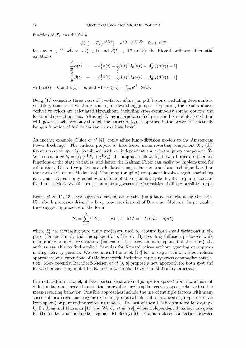
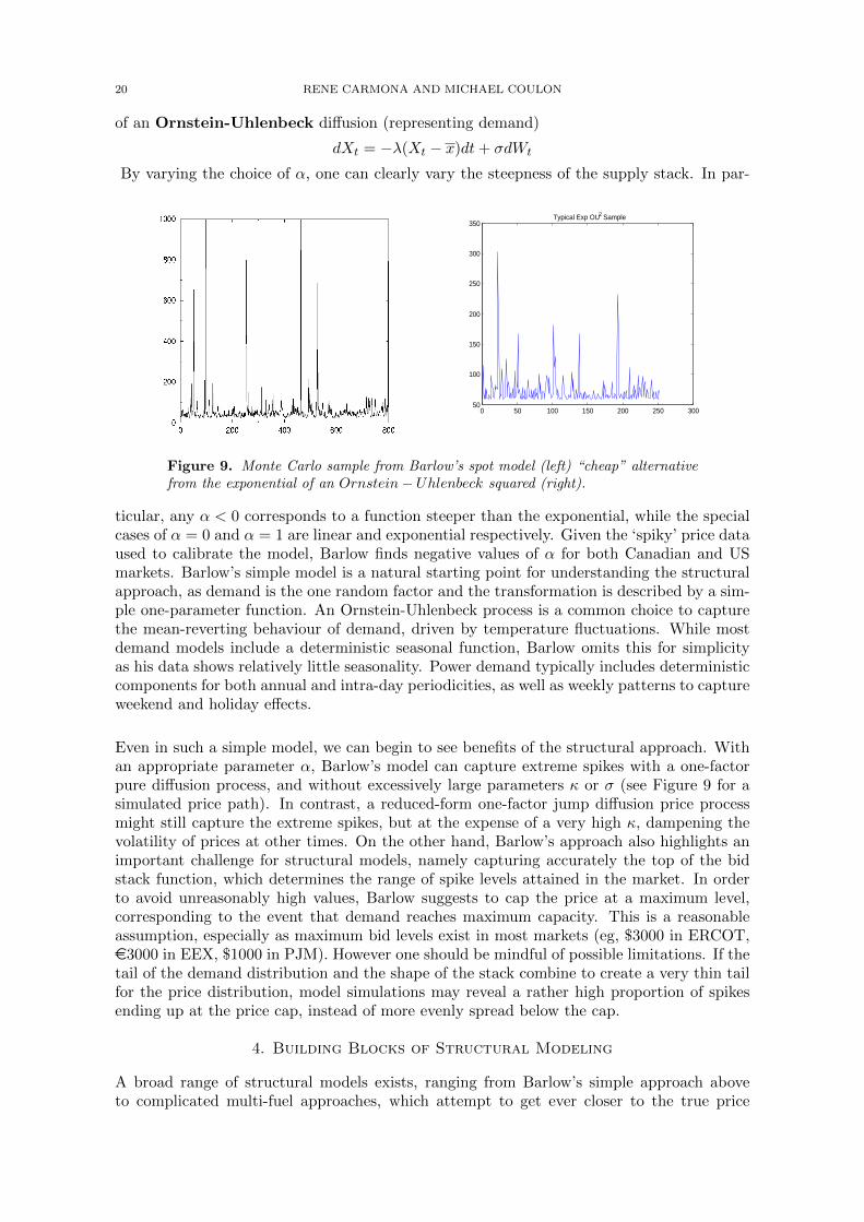
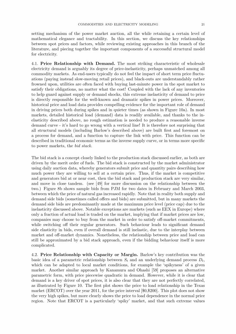
Given the complexities of forward curve data, it is perhaps not surprising that the spotprice often serves as the preferred starting point for modellers. Figure 8a gives a time seriesplot of the daily average spot price of electricity on the PJM exchange between 2000 and2010. What we call the spot price is the market clearing price set for each hour in the day-ahead auction. The system operator needs advanced notice to make sure that the schedule
16 RENE CARMONA AND MICHAEL COULON
is feasible and transmission constraints are met. Hence a ‘day-ahead’ price is determinedvia a large optimization problem, but as rebalancing of supply and demand is required upuntil actual delivery, a ‘real-time’ price also exists (and is sometimes referred to as the spotprice). In any case, the type of time evolution shown in Figure 8a has nothing in commonwith equity prices or even other commodity prices. The most obvious difference is the highfrequency of sudden spikes when the price jumps up very quickly before dropping down tonear its previous level in a very short amount of time. As a result, the volatility of the‘returns’ (a questionable term for a non-storable commodity!) is excessively high, say ina range from 50% up to 200% which is very different from the volatility of other financialproducts.
In line with the structural approach described in the next section, we made a definite choiceto answer the question “Which spot price should one use?”. But mathematical models couldalso be developed for the real-time price, the price on the balancing market, the balance-of-the-week price, the balance-of-the-month price, etc. For all these mathematical models tobe consistent, the diversity of candidates begs the question: can a complete forward curvebe constructed (for all T ) and does the forward price then converge to spot as the timeto maturity goes to zero? If this is indeed the case, it would make sense to define the“mathematical spot price” as
S(t) = limT↓t
F (t, T )
as we did in Subsection 2.4, and expect that its statistical properties will coincide with thoseof the day-ahead price chosen as a proxy.
3.1. More Data Peculiarities. Beyond the issues already mentioned (e.g. integrity, spar-sity, etc), one of the most surprising features of electricity prices is the fact that some ofthem are frequently negative. If we consider for example the case of the PJM (Pensylvania,New Jersey, Maryland) region in the North East of the US, every single day, real-time andday-ahead prices as well as hour by hour load prediction for the following day are publishedfor over 3, 000 nodes in the transmission network, and many negative prices can be found.For example, in 2003 over 100, 000 such hourly instances occurred across the grid. Theycome in geographic clusters, at special times of the year (shoulder months) and times ofthe day (night and early morning). The first suspects are obviously errors in predictions ofthe load, and high temperature volatilities. More sophisticated explanations involve networktransmission and congestion, causing an oversupply in one location and an undersupply inanother. While we do not want to dwell on the issue of negative prices, it is a useful exampleto highlight the fact that electricity pricing cannot be done by mere application of techniquesand results developed for the financial markets, and that the physical nature of the com-modity, its demand patterns and the idiosyncrasies of its production and transmission needto be taken into account.
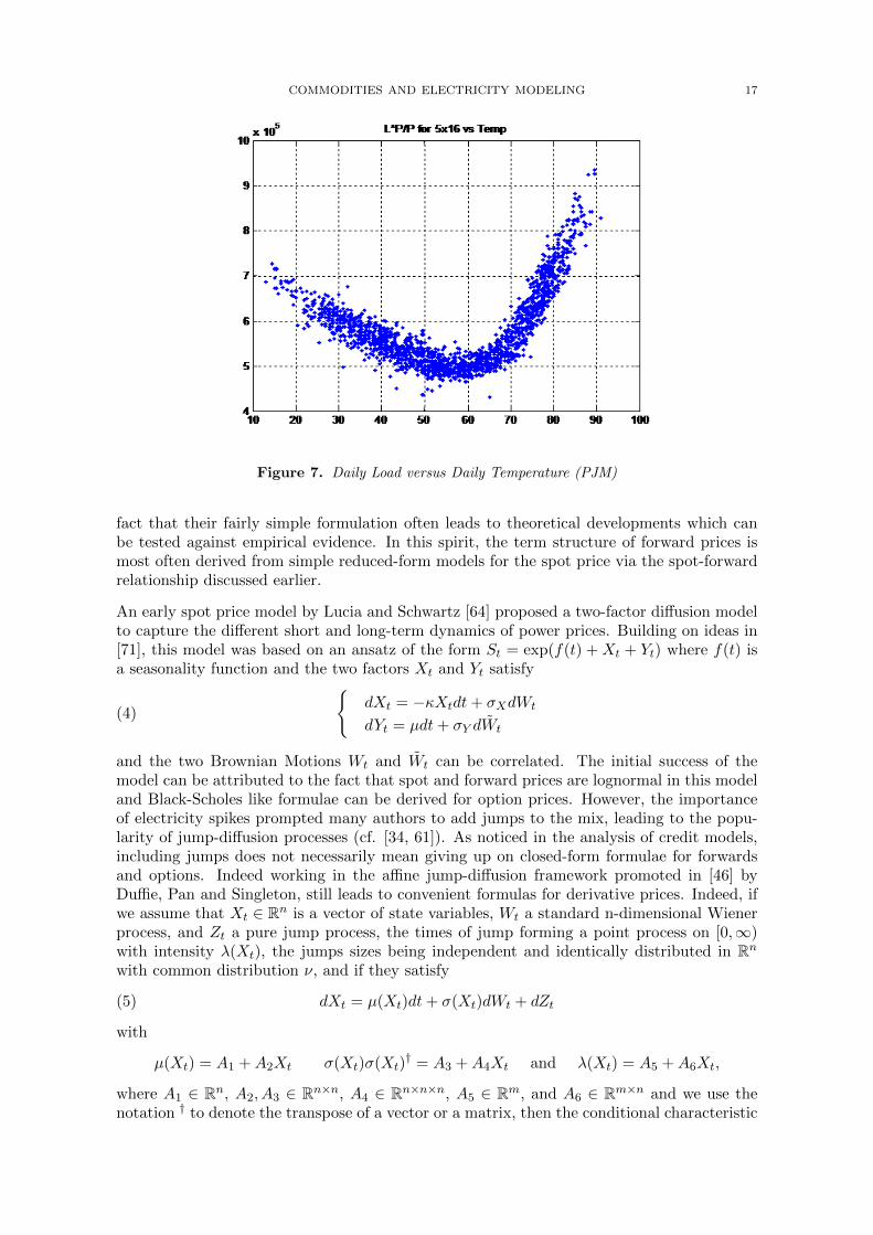
3.2. Modeling the Demand: the Load / Temperature Relationship. As explainedearlier, demand for electricity in the US is in great part driven by weather conditions andespecially temperature. Figure 7 illustrates this fact by showing that a simple regressioncan be used to predict the demand for electricity as a function of the temperature. As aresult, weather dynamics need to be included in pricing and this adds another source ofincompleteness to the mathematical models.
3.3. Reduced-Form Models. By nature, reduced-form models try to identify stylizedproperties of electricity prices, and capture them in simple relationships from which deriva-tive prices can be obtained, preferably through analytic formulae. So instead of modeling thefundamentals of supply and demand and having prices appear as the result of equilibriumconsiderations, reduced-form models strive for tractability, and for this reason, they usuallyinvolve a small number of factors and parameters. The source of their popularity is the
COMMODITIES AND ELECTRICITY MODELING 17
Figure 7. Daily Load versus Daily Temperature (PJM)
fact that their fairly simple formulation often leads to theoretical developments which canbe tested against empirical evidence. In this spirit, the term structure of forward prices ismost often derived from simple reduced-form models for the spot price via the spot-forwardrelationship discussed earlier.
An early spot price model by Lucia and Schwartz [64] proposed a two-factor diffusion modelto capture the different short and long-term dynamics of power prices. Building on ideas in[71], this model was based on an ansatz of the form St = exp(f(t) + Xt + Yt) where f(t) isa seasonality function and the two factors Xt and Yt satisfy
(4)
{dXt = −κXtdt+ σXdWt
dYt = µdt+ σY dWt
and the two Brownian Motions Wt and Wt can be correlated. The initial success of themodel can be attributed to the fact that spot and forward prices are lognormal in this modeland Black-Scholes like formulae can be derived for option prices. However, the importanceof electricity spikes prompted many authors to add jumps to the mix, leading to the popu-larity of jump-diffusion processes (cf. [34, 61]). As noticed in the analysis of credit models,including jumps does not necessarily mean giving up on closed-form formulae for forwardsand options. Indeed working in the affine jump-diffusion framework promoted in [46] byDuffie, Pan and Singleton, still leads to convenient formulas for derivative prices. Indeed, ifwe assume that Xt ∈ Rn is a vector of state variables, Wt a standard n-dimensional Wienerprocess, and Zt a pure jump process, the times of jump forming a point process on [0,∞)with intensity λ(Xt), the jumps sizes being independent and identically distributed in Rnwith common distribution ν, and if they satisfy
(5) dXt = µ(Xt)dt+ σ(Xt)dWt + dZt
with
µ(Xt) = A1 +A2Xt σ(Xt)σ(Xt)† = A3 +A4Xt and λ(Xt) = A5 +A6Xt,
where A1 ∈ Rn, A2, A3 ∈ Rn×n, A4 ∈ Rn×n×n, A5 ∈ Rm, and A6 ∈ Rm×n and we use thenotation † to denote the transpose of a vector or a matrix, then the conditional characteristic
18 RENE CARMONA AND MICHAEL COULON
function of Xt has the form
ψ(u) = Et[eu†XT ] = eα(t)+β(t)†Xt for t ≤ T
for any u ∈ C, where α(t) ∈ R and β(t) ∈ Rn satisfy the Riccati ordinary differentialequations
d
dtα(t) = −A†1β(t)− 1
2β(t)†A3β(t)−A†5[ζ(β(t))− 1]
d
dtβ(t) = −A†2β(t)− 1
2β(t)†A4β(t)−A†6[ζ(β(t))− 1]
with α(t) = 0 and β(t) = u, and where ζ(c) =∫Rn e
c†zdv(z).
Deng [45] considers three cases of two-factor affine jump-diffusions, including deterministicvolatility, stochastic volatility and regime-switching jumps. Exploiting the results above,derivative prices are calculated throughout, including cross-commodity spread options andlocational spread options. Although Deng incorporates fuel prices in his models, correlationwith power is achieved only through the matrix σ(Xt), as opposed to the power price actuallybeing a function of fuel prices (as we shall see later).
As another example, Culot et al [41] apply affine jump-diffusion models to the AmsterdamPower Exchange. The authors propose a three-factor mean-reverting component Xt, (dif-
ferent reversion speeds), combined with an independent three-factor jump component Xt.
With spot price St = exp(γ†Xt + γ†Xt), this approach allows log forward prices to be affinefunctions of the state variables, and hence the Kalman Filter can easily be implemented forcalibration. Derivative prices are calculated using a Fourier transform technique based onthe work of Carr and Madan [33]. The jump (or spike) component involves regime-switching
ideas, as γ†Xt can only equal zero or one of three possible spike levels, so jump sizes arefixed and a Markov chain transition matrix governs the intensities of all the possible jumps.
Benth et al [11, 13] have suggested several alternative jump-based models, using Ornstein-Uhlenbeck processes driven by Levy processes instead of Brownian Motions. In particular,they suggest approaches of the form
St =n∑i=1
wiYit , where dY i
t = −λiY it dt+ σitdL
it
where Lit are increasing pure jump processes, used to capture both small variations in theprice (for certain i), and the spikes (for other i). By avoiding diffusion processes whilemaintaining an additive structure (instead of the more common exponential structure), theauthors are able to find explicit formulas for forward prices without ignoring or approxi-mating delivery periods. We recommend the book [13] for an exposition of various relatedapproaches and extensions of this framework, including capturing cross-commodity correla-tion. More recently, Barndorff-Nielsen et al [9, 8] propose a new approach for both spot andforward prices using ambit fields, and in particular Levy semi-stationary processes.
In a reduced-form model, at least partial separation of jumps (or spikes) from more ‘normal’diffusion factors is needed due to the large difference in spike recovery speed relative to othermean-reverting behavior. Possible approaches include the use of multiple factors with manyspeeds of mean reversion, regime switching jumps (which lead to downwards jumps to recoverfrom spikes) or pure regime switching models. The last of these has been studied for exampleby De Jong and Huisman [43] and Weron et al [79], where independent dynamics are givenfor the ‘spike’ and ‘non-spike’ regime. Kholodnyi [60] retains a closer connection between
COMMODITIES AND ELECTRICITY MODELING 19
the two regimes in his model, instead suggesting that the price jumps from Xt to λXt forsome constant λ when there is a regime switch. Regime switching models benefit from thefact that high prices can last for several time periods (typically just a few hours, so oneshould not interpret the terminology ‘regime’ to mean a lasting paradigm shift), reflectingfor example periods of generator outages. The recovery from an outage can be as suddenas the outage itself, a characteristic difficult to mimic with mean-reverting jump-diffusions.A variation proposed by Geman and Roncoroni [54] is a jump-diffusion model which forcesjumps to be downwards when prices are above a certain threshold.
While many of the models discussed above produce useful results and realistic price dynam-ics, they often face calibration challenges due to the need for multiple unobservable factors,an inability to adapt to changing market conditions, or to the complication of identifyinghistorical spikes (or regimes). In addition, and perhaps more importantly from an industryperspective when managing complex portfolios of assets, they typically fail to capture theimportant correlations between power prices, other energy prices and power demand.
0
100
200
2001 2004 2007 2010Year
Price
($
/MW
h)
(a) Historical daily average prices
0 7
x 104
300
600
Supply (MW)
Price
($
/MW
h)
1st February 20031st March 2003
(b) Sample bid stacks
Figure 8. Historical prices and bids from the PJM market in the North East US
3.4. A First Structural Model for Spot Prices. For electricity as for all other com-modities, the balancing act between supply and demand in the price formation leads tomean reversion of prices towards costs of production. Furthermore, the relationships be-tween underlying supply and demand factors in electricity markets are more observable andbetter understood than in other markets. This has naturally led to the development ofso-called structural models. In this category, the first real proposal for a tractable spot pric-ing model based on a supply/demand argument is due to Martin Barlow [7] and we reviewbriefly the main components of his pricing model. Motivated by observed auction data, Bar-low proposed to use a vertical demand curve (reminiscent of the inelasticity of the demandfor electricity) and a supply curve given by a nonlinear function of a simple diffusion process:
S(t) =
{fα(Xt) 1 + αXt > ε0
ε1/α0 1 + αXt ≤ ε0
for the non-linear function
fα(x) =
{(1 + αx)1/α, α 6= 0
ex α = 0
20 RENE CARMONA AND MICHAEL COULON
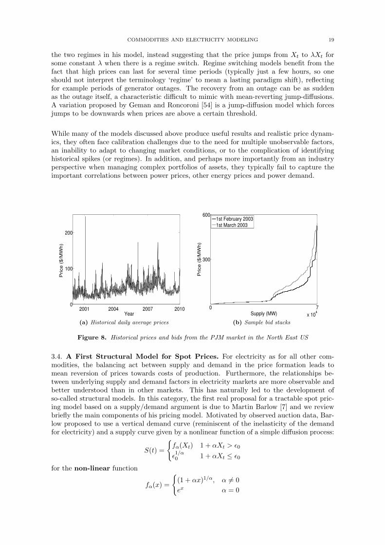
of an Ornstein-Uhlenbeck diffusion (representing demand)
dXt = −λ(Xt − x)dt+ σdWt
By varying the choice of α, one can clearly vary the steepness of the supply stack. In par-
0 50 100 150 200 250 30050
100
150
200
250
300
350Typical Exp OU2 Sample
Figure 9. Monte Carlo sample from Barlow’s spot model (left) “cheap” alternativefrom the exponential of an Ornstein− Uhlenbeck squared (right).
ticular, any α < 0 corresponds to a function steeper than the exponential, while the specialcases of α = 0 and α = 1 are linear and exponential respectively. Given the ‘spiky’ price dataused to calibrate the model, Barlow finds negative values of α for both Canadian and USmarkets. Barlow’s simple model is a natural starting point for understanding the structuralapproach, as demand is the one random factor and the transformation is described by a sim-ple one-parameter function. An Ornstein-Uhlenbeck process is a common choice to capturethe mean-reverting behaviour of demand, driven by temperature fluctuations. While mostdemand models include a deterministic seasonal function, Barlow omits this for simplicityas his data shows relatively little seasonality. Power demand typically includes deterministiccomponents for both annual and intra-day periodicities, as well as weekly patterns to captureweekend and holiday effects.
Even in such a simple model, we can begin to see benefits of the structural approach. Withan appropriate parameter α, Barlow’s model can capture extreme spikes with a one-factorpure diffusion process, and without excessively large parameters κ or σ (see Figure 9 for asimulated price path). In contrast, a reduced-form one-factor jump diffusion price processmight still capture the extreme spikes, but at the expense of a very high κ, dampening thevolatility of prices at other times. On the other hand, Barlow’s approach also highlights animportant challenge for structural models, namely capturing accurately the top of the bidstack function, which determines the range of spike levels attained in the market. In orderto avoid unreasonably high values, Barlow suggests to cap the price at a maximum level,corresponding to the event that demand reaches maximum capacity. This is a reasonableassumption, especially as maximum bid levels exist in most markets (eg, $3000 in ERCOT,e3000 in EEX, $1000 in PJM). However one should be mindful of possible limitations. If thetail of the demand distribution and the shape of the stack combine to create a very thin tailfor the price distribution, model simulations may reveal a rather high proportion of spikesending up at the price cap, instead of more evenly spread below the cap.
4. Building Blocks of Structural Modeling
A broad range of structural models exists, ranging from Barlow’s simple approach aboveto complicated multi-fuel approaches, which attempt to get ever closer to the true price
COMMODITIES AND ELECTRICITY MODELING 21
setting mechanism of the power market auction, all the while retaining a certain level ofmathematical elegance and tractability. In this section, we discuss the key relationshipsbetween spot prices and factors, while reviewing existing approaches in this branch of theliterature, and piecing together the important components of a successful structural modelfor electricity.
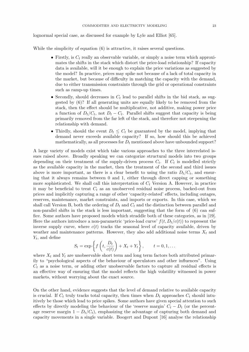
4.1. Price Relationship with Demand. The most striking characteristic of wholesaleelectricity demand is arguably its degree of price-inelasticity, perhaps unmatched among allcommodity markets. As end-users typically do not feel the impact of short term price fluctu-ations (paying instead slow-moving retail prices), and black-outs are understandably ratherfrowned upon, utilities are often faced with buying last-minute power in the spot market tosatisfy their obligations, no matter what the cost! Coupled with the lack of any inventoriesto help guard against supply or demand shocks, this extreme inelasticity of demand to priceis directly responsible for the well-known and dramatic spikes in power prices. Moreover,historical price and load data provides compelling evidence for the important role of demandin driving prices both during spikes and in quieter times (as shown in Figure 10a). In mostmarkets, detailed historical load (demand) data is readily available, and thanks to the in-elasticity described above, no rough estimation is needed to produce a reasonable inversedemand curve - it’s hard to go wrong with a vertical line! It is therefore not surprising thatall structural models (including Barlow’s described above) are built first and foremost ona process for demand, and a function to capture the link with price. This function can bedescribed in traditional economic terms as the inverse supply curve, or in terms more specificto power markets, the bid stack.
The bid stack is a concept closely linked to the production stack discussed earlier, as both aredriven by the merit order of fuels. The bid stack is constructed by the market administratorusing daily auction data, whereby generators submit price and quantity pairs describing howmuch power they are willing to sell at a certain price. Thus, if the market is competitiveand generators bid at or near cost, then the bid stack and production stack are very similar,and move in close tandem. (see [49] for more discussion on the relationship between thetwo.) Figure 8b shows sample bids from PJM for two dates in February and March 2003,between which the price of natural gas increased rapidly. Note that in reality both supply anddemand side bids (sometimes called offers and bids) are submitted, but in many markets thedemand side bids are predominantly made at the maximum price level (price cap) due to theinelasticity discussed above. Notable exceptions are markets (such as EEX in Europe) whereonly a fraction of actual load is traded on the market, implying that if market prices are low,companies may choose to buy from the market in order to satisfy off-market commitments,while switching off their regular generators. Such behaviour leads to significant demandside elasticity in bids, even if overall demand is still inelastic, due to the interplay betweenmarket and off-market dynamics. Nonetheless, the relationship between price and load canstill be approximated by a bid stack approach, even if the bidding behaviour itself is morecomplicated.
4.2. Price Relationship with Capacity or Margin. Barlow’s key contribution was thebasic idea of a parametric relationship between St and an underlying demand process Dt,which can be adapted to local market conditions, for example the ‘spikyness’ of a givenmarket. Another similar approach by Kanamura and Ohashi [59] proposes an alternativeparametric form, with price piecewise quadratic in demand. However, while it is clear thatdemand is a key driver of spot prices, it is also clear that they are not perfectly correlated,as illustrated by Figure 10. The first plot shows the price to load relationship in the Texasmarket (ERCOT) over the year 2011, for the price interval [$0,$200]. This plot does not showthe very high spikes, but more clearly shows the price to load dependence in the normal priceregion. Note that ERCOT is a particularly ‘spiky’ market, and that such extreme values
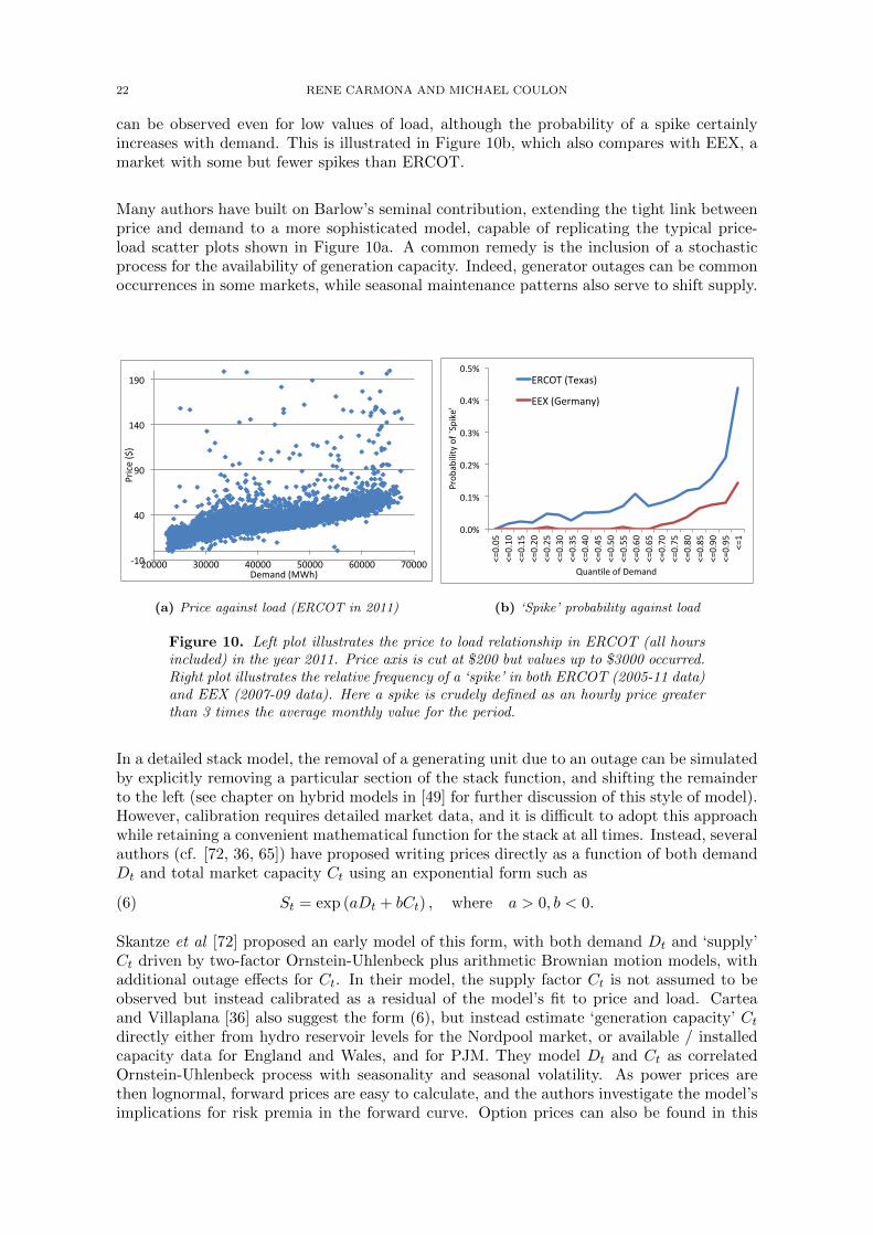
22 RENE CARMONA AND MICHAEL COULON
can be observed even for low values of load, although the probability of a spike certainlyincreases with demand. This is illustrated in Figure 10b, which also compares with EEX, amarket with some but fewer spikes than ERCOT.
Many authors have built on Barlow’s seminal contribution, extending the tight link betweenprice and demand to a more sophisticated model, capable of replicating the typical price-load scatter plots shown in Figure 10a. A common remedy is the inclusion of a stochasticprocess for the availability of generation capacity. Indeed, generator outages can be commonoccurrences in some markets, while seasonal maintenance patterns also serve to shift supply.
!"#$
%#$
&#$
"%#$
"&#$
'####$ (####$ %####$ )####$ *####$ +####$
,-./0$123$
405678$19:;3$
(a) Price against load (ERCOT in 2011)
!"!#$
!"%#$
!"&#$
!"'#$
!"(#$
!")#$
*+!"!)$
*+!"%!$
*+!"%)$
*+!"&!$
*+!"&)$
*+!"'!$
*+!"')$
*+!"(!$
*+!"()$
*+!")!$
*+!"))$
*+!",!$
*+!",)$
*+!"-!$
*+!"-)$
*+!".!$
*+!".)$
*+!"/!$
*+!"/)$
*+%$
0123
4356578$29$:;<5=>?$
@A4BC6>$29$D>E4BF$
GHIJK$LK>M4NO$
GGP$LQ>1E4B8O$
(b) ‘Spike’ probability against load
Figure 10. Left plot illustrates the price to load relationship in ERCOT (all hoursincluded) in the year 2011. Price axis is cut at $200 but values up to $3000 occurred.Right plot illustrates the relative frequency of a ‘spike’ in both ERCOT (2005-11 data)and EEX (2007-09 data). Here a spike is crudely defined as an hourly price greaterthan 3 times the average monthly value for the period.
In a detailed stack model, the removal of a generating unit due to an outage can be simulatedby explicitly removing a particular section of the stack function, and shifting the remainderto the left (see chapter on hybrid models in [49] for further discussion of this style of model).However, calibration requires detailed market data, and it is difficult to adopt this approachwhile retaining a convenient mathematical function for the stack at all times. Instead, severalauthors (cf. [72, 36, 65]) have proposed writing prices directly as a function of both demandDt and total market capacity Ct using an exponential form such as
(6) St = exp (aDt + bCt) , where a > 0, b < 0.
Skantze et al [72] proposed an early model of this form, with both demand Dt and ‘supply’Ct driven by two-factor Ornstein-Uhlenbeck plus arithmetic Brownian motion models, withadditional outage effects for Ct. In their model, the supply factor Ct is not assumed to beobserved but instead calibrated as a residual of the model’s fit to price and load. Carteaand Villaplana [36] also suggest the form (6), but instead estimate ‘generation capacity’ Ctdirectly either from hydro reservoir levels for the Nordpool market, or available / installedcapacity data for England and Wales, and for PJM. They model Dt and Ct as correlatedOrnstein-Uhlenbeck process with seasonality and seasonal volatility. As power prices arethen lognormal, forward prices are easy to calculate, and the authors investigate the model’simplications for risk premia in the forward curve. Option prices can also be found in this
COMMODITIES AND ELECTRICITY MODELING 23
lognormal special case, as discussed for example by Lyle and Elliot [65].
While the simplicity of equation (6) is attractive, it raises several questions.
• Firstly, is Ct really an observable variable, or simply a noise term which approxi-mates the shifts in the stack which distort the price-load relationship? If capacitydata is available, will it be enough to explain the price variations as suggested bythe model? In practice, prices may spike not because of a lack of total capacity inthe market, but because of difficulty in matching the capacity with the demand,due to either transmission constraints through the grid or operational constraintssuch as ramp-up times.
• Secondly, should decreases in Ct lead to parallel shifts in the bid stack, as sug-gested by (6)? If all generating units are equally likely to be removed from thestack, then the effect should be multiplicative, not additive, making power pricea function of Dt/Ct, not Dt − Ct. Parallel shifts suggest that capacity is beingprimarily removed from the far left of the stack, and therefore not steepening therelationship with demand.
• Thirdly, should the event Dt ≤ Ct be guaranteed by the model, implying thatdemand never exceeds available capacity? If so, how should this be achievedmathematically, as all processes forDt mentioned above have unbounded support?
A large variety of models exist which take various approaches to the three interrelated is-sues raised above. Broadly speaking we can categorize structural models into two groupsdepending on their treatment of the supply-driven process Ct. If Ct is modelled strictlyas the available capacity in the market, then the treatment of the second and third issuesabove is more important, as there is a clear benefit to using the ratio Dt/Ct, and ensur-ing that it always remains between 0 and 1, either through direct capping or somethingmore sophisticated. We shall call this interpretation of Ct Version A. However, in practiceit may be beneficial to treat Ct as an unobserved residual noise process, backed-out fromprices and implicitly capturing a range of other ‘capacity-related’ effects, including outages,reserves, maintenance, market constraints, and imports or exports. In this case, which weshall call Version B, both the ordering of Dt and Ct and the distinction between parallel andnon-parallel shifts in the stack is less important, suggesting that the form of (6) can suf-fice. Some authors have proposed models which straddle both of these categories, as in [19].Here the authors introduce a non-parametric ‘price-load curve’ f(t,Dt/c(t)) to represent theinverse supply curve, where c(t) tracks the seasonal level of capacity available, driven byweather and maintenance patterns. However, they also add additional noise terms Xt andYt, and define
St = exp
{f
(t,Dt
c(t)
)+Xt + Yt
}, t = 0, 1, . . .
where Xt and Yt are unobservable short term and long term factors both attributed primar-ily to “psychological aspects of the behaviour of speculators and other influences”. UsingCt as a noise term, or adding other unobservable factors to capture all residual effects isan effective way of ensuring that the model reflects the high volatility witnessed in powermarkets, without worrying about the exact source.
On the other hand, evidence suggests that the level of demand relative to available capacityis crucial. If Ct truly tracks total capacity, then times when Dt approaches Ct should intu-itively be those which lead to price spikes. Some authors have given special attention to sucheffects by directly modeling the behaviour of the ‘reserve margin’ Ct −Dt (or the percent-age reserve margin 1 − Dt/Ct), emphasizing the advantage of capturing both demand andcapacity movements in a single variable. Boogert and Dupont [16] analyse the relationship
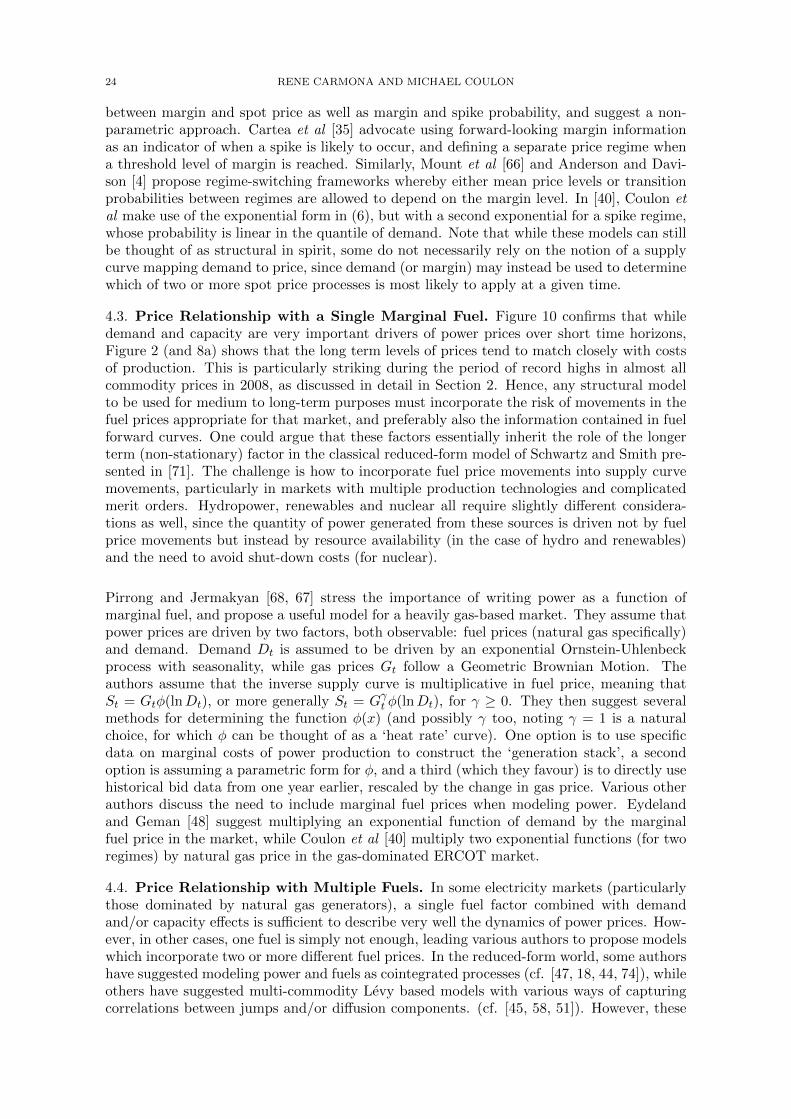
24 RENE CARMONA AND MICHAEL COULON
between margin and spot price as well as margin and spike probability, and suggest a non-parametric approach. Cartea et al [35] advocate using forward-looking margin informationas an indicator of when a spike is likely to occur, and defining a separate price regime whena threshold level of margin is reached. Similarly, Mount et al [66] and Anderson and Davi-son [4] propose regime-switching frameworks whereby either mean price levels or transitionprobabilities between regimes are allowed to depend on the margin level. In [40], Coulon etal make use of the exponential form in (6), but with a second exponential for a spike regime,whose probability is linear in the quantile of demand. Note that while these models can stillbe thought of as structural in spirit, some do not necessarily rely on the notion of a supplycurve mapping demand to price, since demand (or margin) may instead be used to determinewhich of two or more spot price processes is most likely to apply at a given time.
4.3. Price Relationship with a Single Marginal Fuel. Figure 10 confirms that whiledemand and capacity are very important drivers of power prices over short time horizons,Figure 2 (and 8a) shows that the long term levels of prices tend to match closely with costsof production. This is particularly striking during the period of record highs in almost allcommodity prices in 2008, as discussed in detail in Section 2. Hence, any structural modelto be used for medium to long-term purposes must incorporate the risk of movements in thefuel prices appropriate for that market, and preferably also the information contained in fuelforward curves. One could argue that these factors essentially inherit the role of the longerterm (non-stationary) factor in the classical reduced-form model of Schwartz and Smith pre-sented in [71]. The challenge is how to incorporate fuel price movements into supply curvemovements, particularly in markets with multiple production technologies and complicatedmerit orders. Hydropower, renewables and nuclear all require slightly different considera-tions as well, since the quantity of power generated from these sources is driven not by fuelprice movements but instead by resource availability (in the case of hydro and renewables)and the need to avoid shut-down costs (for nuclear).
Pirrong and Jermakyan [68, 67] stress the importance of writing power as a function ofmarginal fuel, and propose a useful model for a heavily gas-based market. They assume thatpower prices are driven by two factors, both observable: fuel prices (natural gas specifically)and demand. Demand Dt is assumed to be driven by an exponential Ornstein-Uhlenbeckprocess with seasonality, while gas prices Gt follow a Geometric Brownian Motion. Theauthors assume that the inverse supply curve is multiplicative in fuel price, meaning thatSt = Gtφ(lnDt), or more generally St = Gγt φ(lnDt), for γ ≥ 0. They then suggest severalmethods for determining the function φ(x) (and possibly γ too, noting γ = 1 is a naturalchoice, for which φ can be thought of as a ‘heat rate’ curve). One option is to use specificdata on marginal costs of power production to construct the ‘generation stack’, a secondoption is assuming a parametric form for φ, and a third (which they favour) is to directly usehistorical bid data from one year earlier, rescaled by the change in gas price. Various otherauthors discuss the need to include marginal fuel prices when modeling power. Eydelandand Geman [48] suggest multiplying an exponential function of demand by the marginalfuel price in the market, while Coulon et al [40] multiply two exponential functions (for tworegimes) by natural gas price in the gas-dominated ERCOT market.
4.4. Price Relationship with Multiple Fuels. In some electricity markets (particularlythose dominated by natural gas generators), a single fuel factor combined with demandand/or capacity effects is sufficient to describe very well the dynamics of power prices. How-ever, in other cases, one fuel is simply not enough, leading various authors to propose modelswhich incorporate two or more different fuel prices. In the reduced-form world, some authorshave suggested modeling power and fuels as cointegrated processes (cf. [47, 18, 44, 74]), whileothers have suggested multi-commodity Levy based models with various ways of capturingcorrelations between jumps and/or diffusion components. (cf. [45, 58, 51]). However, these
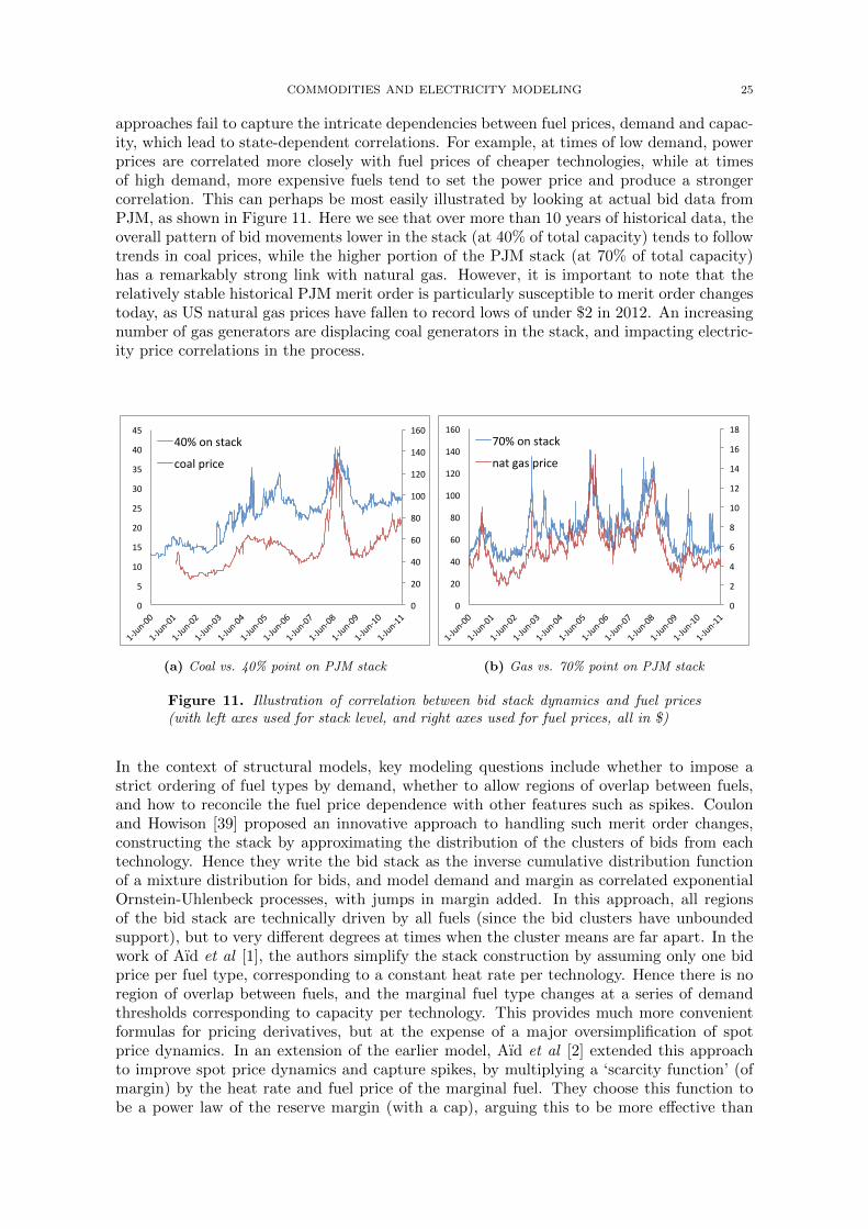
COMMODITIES AND ELECTRICITY MODELING 25
approaches fail to capture the intricate dependencies between fuel prices, demand and capac-ity, which lead to state-dependent correlations. For example, at times of low demand, powerprices are correlated more closely with fuel prices of cheaper technologies, while at timesof high demand, more expensive fuels tend to set the power price and produce a strongercorrelation. This can perhaps be most easily illustrated by looking at actual bid data fromPJM, as shown in Figure 11. Here we see that over more than 10 years of historical data, theoverall pattern of bid movements lower in the stack (at 40% of total capacity) tends to followtrends in coal prices, while the higher portion of the PJM stack (at 70% of total capacity)has a remarkably strong link with natural gas. However, it is important to note that therelatively stable historical PJM merit order is particularly susceptible to merit order changestoday, as US natural gas prices have fallen to record lows of under $2 in 2012. An increasingnumber of gas generators are displacing coal generators in the stack, and impacting electric-ity price correlations in the process.
!"
#!"
$!"
%!"
&!"
'!!"
'#!"
'$!"
'%!"
!"
("
'!"
'("
#!"
#("
)!"
)("
$!"
$("
'*+,-*!!"
'*+,-*!'"
'*+,-*!#"
'*+,-*!)"
'*+,-*!$"
'*+,-*!("
'*+,-*!%"
'*+,-*!."
'*+,-*!&"
'*+,-*!/"
'*+,-*'!"
'*+,-*''"
$!0"1-"23456"
5147"89:5;"
(a) Coal vs. 40% point on PJM stack
!"
#"
$"
%"
&"
'!"
'#"
'$"
'%"
'&"
!"
#!"
$!"
%!"
&!"
'!!"
'#!"
'$!"
'%!"
'()*+(!!"
'()*+(!'"
'()*+(!#"
'()*+(!,"
'()*+(!$"
'()*+(!-"
'()*+(!%"
'()*+(!."
'()*+(!&"
'()*+(!/"
'()*+('!"
'()*+(''"
.!0"1+"23456"
+43"742"89:5;"
(b) Gas vs. 70% point on PJM stack
Figure 11. Illustration of correlation between bid stack dynamics and fuel prices(with left axes used for stack level, and right axes used for fuel prices, all in $)
In the context of structural models, key modeling questions include whether to impose astrict ordering of fuel types by demand, whether to allow regions of overlap between fuels,and how to reconcile the fuel price dependence with other features such as spikes. Coulonand Howison [39] proposed an innovative approach to handling such merit order changes,constructing the stack by approximating the distribution of the clusters of bids from eachtechnology. Hence they write the bid stack as the inverse cumulative distribution functionof a mixture distribution for bids, and model demand and margin as correlated exponentialOrnstein-Uhlenbeck processes, with jumps in margin added. In this approach, all regionsof the bid stack are technically driven by all fuels (since the bid clusters have unboundedsupport), but to very different degrees at times when the cluster means are far apart. In thework of Aıd et al [1], the authors simplify the stack construction by assuming only one bidprice per fuel type, corresponding to a constant heat rate per technology. Hence there is noregion of overlap between fuels, and the marginal fuel type changes at a series of demandthresholds corresponding to capacity per technology. This provides much more convenientformulas for pricing derivatives, but at the expense of a major oversimplification of spotprice dynamics. In an extension of the earlier model, Aıd et al [2] extended this approachto improve spot price dynamics and capture spikes, by multiplying a ‘scarcity function’ (ofmargin) by the heat rate and fuel price of the marginal fuel. They choose this function tobe a power law of the reserve margin (with a cap), arguing this to be more effective than
26 RENE CARMONA AND MICHAEL COULON
the common choice of exponential. While the choice of marginal fuel is still determinedby demand, they sacrifice the possibility of merit order changes, by assuming the orderingof fuels is fixed initially, arguing that this is reasonable over short horizons. Carmona etal [21] propose instead a framework based on different exponential bid curves for each fuel(corresponding intuitively to the range of heat rates per technology), and combine theseprecisely as the merit order dictates to produce a piecewise exponential function for themarket as a whole. Hence demand thresholds exist where marginal fuel type(s) changes,but these are highly dynamic, with overlap regions appearing and disappearing in the stack,and the merit order changing as fuel prices move. The model is particularly convenient forthe two-fuel case as closed-form expressions exist for forwards and spread options. However,it is fair to say that for three or more fuels the calculations become unmanageable. Inthe following section, we will present a broad multi-fuel structural framework which buildsperhaps most closely on the last of these models, but draws on ideas from all existing workdiscussed here. Note that for simplicity we do not include carbon emissions prices into ourstructural framework here, and instead refer the interested reader to [22, 42, 56] for stack-based models which include carbon emissions prices as additional production costs, typicallyin conjunction with multiple fuel types with different emissions rates.
5. Forward Pricing in a Structural Approach
While reduced-form models are often designed specifically to facilitate derivative pricing(including those mentioned in Section 3.3), structural models often face a choice betweenstaying true to the market’s structure and cutting some corners to price forwards or op-tions efficiently. Ideally, a model should capture the structural relationships accurately whileretaining convenient expressions for derivatives, but in some markets this may be very chal-lenging indeed. As forward contracts are by far the most widely and liquidly traded contracts,allowing for rapid calibration to the observed forward curve is typically a top priority for anymodel, while convenient option pricing results are a welcome bonus but secondary concern.In this section, we discuss the challenges of derivative pricing in structural models, and sug-gest general frameworks which allow for the explicit calculation of at least forward prices.(In some special cases, options and other derivatives can be priced, as discussed for powerplant valuation in [21], but we do not investigate this here.)
As several authors have discussed (cf. [21, 1, 39]), one advantage of using structural pricemodels for pricing forwards is to capture the dependence of electricity forwards on fuelforwards in a manner which is consistent with their stack-based relationship in the spot mar-ket. Another advantage is to capture forward-looking information about upcoming marketchanges, such as a changing generation mix (e.g. increased renewables, technological devel-opments, the nuclear moratorium in Germany, etc.), or the introduction of new regulation(e.g. emissions markets, market coupling). Finally, one might wish to include a view on loadgrowth or upcoming maintenance schedules. No matter the motivation, the core goal hereis to choose a flexible and realistic functional relationship between price and its underlyingdrivers, such that expectations of future spot prices can be explicitly calculated, and henceforward prices found.
Let F p(t, T ) denote the forward price of electricity at time t for delivery at time T . Recallthat F p(t, T ) = Et[ST ] where Et[·] denotes the conditional expectation given time t informa-tion with respect to a risk neutral probability measure. (We assume this measure is given,and relegate a discussion of risk premia to Section 5.3.) The same equation holds for fuelprices, so for example we write F g(t, T ) = Et[SgT ] for the forward price of gas.
COMMODITIES AND ELECTRICITY MODELING 27
Our aim is to build a general framework that draws on techniques introduced in a numberof different papers, highlighting the assumptions needed to provide closed-form expressionsfor forward prices. We will make use of the following ingredients:
• Lognormal fuel spot prices - This assumption is a very common and natural choicefor modeling energy (non-power) prices. Geometric Brownian Motion (GBM)with constant convenience yield, the classical exponential Ornstein-Uhlenbeckmodel of Schwartz [70], and its two-factor extensions [71, 55] all satisfy the log-normality assumption, as does the general forward curve model given in (2).
• Power price multiplicative in marginal fuel - This assumption is made by manyauthors (cf. [48, 68, 21, 2] among others), and reflects the fact that fuel costsare the dominant drivers of power bids, and large compared to other operationalcosts. The power price can be thought of as a product of the marginal fuel costand a ‘heat rate function’, describing the heat rate of the marginal generator atthe appropriate demand level. The more possible marginal fuels in a market, thegreater the challenge in building a structural model!
• Gaussian demand (and possibly ‘capacity’) - Power demand is often assumed tobe Gaussian and modelled as an Ornstein-Uhlenbeck process (cf. [7, 36, 65, 59]among others). This is consistent with the (piecewise) linear dependence we high-lighted in the discussion surrounding Figure 7, and the fact that temperature isreasonably well modelled by a Gaussian autoregressive model with strong seasonalcomponents. Depending on the role and treatment of capacity, the process mayneed to be strictly capped at the top and bottom of the stack, or alternatively anadditional Gaussian noise term may be added to represent capacity changes.
• Exponential heat rate functions - The relationship between price and load is typ-ically convex and often modelled with an exponential function, as discussed inSubsection 4.1. Coupled with Gaussian demand, this set-up can provide conve-nient flexibility to produce specialized results.
• Multiple spot price regimes - The assumptions listed above are typically not suf-ficient to capture the heavy-tailed nature of spot prices, with both positive andnegative spikes possible. Various authors have proposed regime-switching mod-els (cf. [43, 79, 66, 4] among others) to handle this primary feature of powerprices. While some of these are pure reduced-form approaches, others mergeregime-switching with a structural framework.
5.1. Single Fuel Markets. We begin with a single fuel model, suitable for markets in whichthe marginal generator is almost always of the same fuel type. Note that generators whichalways bid at very low price levels (or simply at zero) can be incorporated into this frame-work most easily by replacing the demand process Dt by the residual demand process aftersubtracting their capacity. This is particularly relevant for generation types such as nuclearand renewables. Note that this does not mean that these generators are simply ignored, asthe adjustment to model residual demand may require some care, as discussed for wind andsolar power in Germany in [76]. For example the volatility of wind availability may meanthat the residual demand distribution has a significantly higher volatility than the originaldemand distribution. Hence, while it is assumed these units don’t set the power price, theymay well influence the power price. For simplicity, we shall call the unique marginal fuelnatural gas, with spot price denoted Sgt . We now divide our framework into two types ofmodels, which differ in their treatment of capacity Ct. Version A will treat Ct as strictly theavailable generation capacity in the market, while Version B will treat Ct more loosely as astochastic perturbation driven by capacity changes.
28 RENE CARMONA AND MICHAEL COULON
Throughout, we consider one particular maturity of interest, T , and specify the conditionaldistributions (given time t information) of gas price as lognormal, and both demand andcapacity as normal and possibly correlated. We assume the fuel price to be independent ofdemand and capacity. This is a reasonable assumption as power demand is typically drivenpredominantly by temperature, which fluctuates at a faster time scale and depends more onlocal or regional conditions than fuel prices. In summary, the random factors determiningST are
(7)
[DT | Dt
CT | Ct
]∼ N
([µdµc
],
[σ2d ρσdσc
ρσdσc σ2c
]), logSgT | S
gt ∼ N(µg, σ
2g)
Indeed, we stress that we are interested in making minimal assumptions on the behaviour ofthese factors, as different markets may have different characteristics, and different authorsmay favour different Gaussian processes, seasonal patterns and other variations. Our em-phasis is instead primarily on the stack-based mapping to power prices.
Useful Notation and Results:
The calculation of forward prices throughout this section relies on the computation of vari-ous integrals over the multivariate Gaussian density, and thus repeatedly makes use of thefollowing standard result:
(8)
∫ h
−∞ecxΦ
(a+ bx
d
)e−
12x2
√2π
dx = e12c2Φ2
(h− c, a+ bc√
b2 + d2;−b√b2 + d2
)where a, b, c, d, h are constants (with h = ∞ in some cases), and Φ(·) and Φ2(·, ·; ρ) the cu-mulative distribution functions of the univariate and bivariate (correlation ρ) standard (i.e.mean zero and variance one) Gaussian distributions respectively. Note that the constant dis redundant in the expression above, but in practice it is convenient to use this form.
In addition, in some multi-fuel cases, we may require integrating over a bivariate Gaussiandistribution function, in which case the following related result is used:∫ h
−∞ecxΦ2
(a1 + b1x
d1,a2 + b2x
d2;λ
)1√2π
e−12x2dx
= e12c2Φ3
h− c, a1 + b1c√b21 + d2
1
,a2 + b2c√b22 + d2
2
;
1 ρ12 ρ13
ρ12 1 ρ23
ρ13 ρ23 1
(9)
where a1, a2, b1, b2, c, d1, d2, h, λ are constants (with h =∞ in some cases), Φ3(·, ·, ·; Σ) is thestandard trivariate Gaussian cumulative distribution function with correlation matrix Σ, and
ρ12 =−b1√b21 + d2
1
, ρ13 =−b2√b22 + d2
2
, ρ23 =b1b2 + λd1d2√
(b21 + d21)(b22 + d2
2).
Finally, given the frequency of integrating between two finite limits and obtaining a differ-ence between Gaussian cumulative distribution functions, we introduce the following usefulshorthand notation:
Φ2
([x1
x2
], y; ρ
):= Φ2(x1, y; ρ)− Φ2(x2, y; ρ).
5.1.1. Version A:. In a model for which Ct is strictly the maximum capacity in the market, werequire 0 ≤ Dt ≤ Ct, and define a functional form for the bid stack over this range. However,allowing for the possibility of multiple, say N , price regimes (e.g., a normal regime, spikeregime, negative price regime), we define multiple functional forms and attach probabilitiespi (for i = 1, . . . , N) to being in each regime. As evidence suggests that the likelihood of a
COMMODITIES AND ELECTRICITY MODELING 29
spike is load-dependent but spikes do occasionally occur even for low load (see Figure 10),we allow also for load dependent probabilities pi(Dt) as suggested in [40]. Since electricityspot prices are discrete time processes (typically taking 24 values per day, one for each hour,and with relatively weak links between neighboring hours due to non-storability), we donot necessarily need to define a continuous time Markov chain to drive transitions betweenregimes. However, for modeling purposes, one can choose to interpret electricity prices as thediscrete time observation of a hidden continuous time process (see [13] for more discussion)in which case the probabilities here could be the result of a rapidly moving continuous timeMarkov Chain, which approximately reaches its stationary distribution in less than an hour.More generally, we could also allow for pi to depend on the current regime (e.g. for spikeswhich last several hours) but we do not consider this complication here, as capturing thetiming of clusters of spike values is not our priority. In our current model, the spot powerprice St at any t is given by
(10) St = (−1)δi(Sgt )δi exp(αi + βiDt
)with probability pi(Dt)
where Dt = max (0,min(Ct, Dt)) is capped demand. The parameters δi, δi ∈ {0, 1} allow forswitching on and off fuel price dependence and negative prices respectively, and
pi(Dt) = pi + piΦ
(Dt − µdσd
(−1)δi)
for i = 1, . . . , N − 1,(11)
and pN (Dt) = 1−N−1∑i=1
pi(Dt).
For the N -th regime (with is most intuitively thought of as the ‘normal’ regime when noextreme events occur), we can write its probability in the same form as all other regimes:
(12) pN (Dt) = pN + pNΦ
(Dt − µdσd
(−1)δN)
where, defining the sets I = {i : δi = 0} and J = {1, . . . , N − 1} \ I, we have
pN = 1−N−1∑i=1
pi −∑i∈J
pi
pN =∑i∈J
pi −∑i∈I
pi
δN = 0
We require pi(Dt) ∈ (0, 1) for all Dt and all i = 1, . . . , N , which is guaranteed if∑N−1
i=1 (pi +pi) < 1. Note that the probabilities pi(Dt) are chosen to be linear functions of the quantile
of the demand at time t (or of the quantile of −Dt if δi = 1). Intuitively, for a ‘spike’
regime with δi = 0 (and relatively high αi and/or βi), the likelihood of being in such aregime increases gradually with load, from pi up to a maximum of pi + pi. On the other
hand, for a negative price regime with δi = 1, the likelihood decreases steadily with load.The use of the quantile of load is both convenient mathematically and supported by em-pirical evidence (see Figure 10b), although for some markets a piecewise linear function ofthe quantile seems more appropriate (and still leads to closed-form formulas, just a littlemessier!). Finally, note that we expect δi = 1 for the ‘normal’ regime(s) where the priceis most typically set, but may prefer to set δi = 0 for other regimes such as the negativeprice regime since the size of a downwards spike is unlikely to depend on the current gas price.
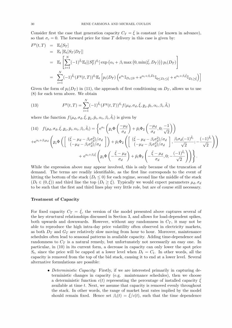
30 RENE CARMONA AND MICHAEL COULON
Consider first the case that generation capacity CT = ξ is constant (or known in advance),so that σc = 0. The forward price for time T delivery in this case is given by:
F p(t, T ) = Et[ST ]
= Et [Et[ST |DT ]]
= Et
[N∑i=1
(−1)δiEt[(SgT )δi ] exp(αi + βi max
(0,min(ξ, DT )
))pi(DT )
]
=N∑i=1
(−1)δi(F g(t, T ))δiEt[pi(DT )
(eαiIDt≤0 + eαi+βiDtI0≤Dt≤ξ + eαi+βiξIDt≥ξ
)]Given the form of pi(DT ) in (11), the approach of first conditioning on DT , allows us to use(8) for each term above. We obtain
(13) F p(t, T ) =N∑i=1
(−1)δi(F g(t, T ))δif(µd, σd, ξ, pi, pi, αi, βi, δi)
where the function f(µd, σd, ξ, pi, pi, αi, βi, δi) is given by
(14) f(µd, σd, ξ, pi, pi, αi, βi, δi) =
{eαi(
piΦ
(−µdσd
)+ piΦ2
(−µdσd
, 0;−1√
2
))+eαi+βiµd
(piΦ
([(ξ − µd − βiσ2
d)/σd(−µd − βiσ2
d)/σd
])+ piΦ2
([(ξ − µd − βiσ2
d)/σd(−µd − βiσ2
d)/σd
],βiσd(−1)δi√
2;−(−1)δi√
2
))
+ eαi+βiξ
(piΦ
(− ξ − µd
σd
)+ piΦ2
(− ξ − µd
σd, 0;−(−1)δi√
2
))}.
While the expression above may appear involved, this is only because of the truncation ofdemand. The terms are readily identifiable, as the first line corresponds to the event ofhitting the bottom of the stack (Dt ≤ 0) for each regime, second line the middle of the stack(Dt ∈ (0, ξ)) and third line the top (Dt ≥ ξ). Typically we would expect parameters µd, σdto be such that the first and third lines play very little role, but are of course still necessary.
Treatment of Capacity
For fixed capacity CT = ξ, the version of the model presented above captures several ofthe key structural relationships discussed in Section 3, and allows for load-dependent spikes,both upwards and downwards. However, without any randomness in CT , it may not beable to reproduce the high intra-day price volatility often observed in electricity markets,as both DT and GT are relatively slow moving from hour to hour. Moreover, maintenanceschedules often lead to seasonal patterns in available capacity. Adding time-dependence andrandomness to CT is a natural remedy, but unfortunately not necessarily an easy one. Inparticular, in (10) in its current form, a decrease in capacity can only lower the spot priceSt, since the price will be capped at a lower level when Dt = Ct. In other words, all thecapacity is removed from the top of the bid stack, causing it to end at a lower level. Severalalternative formulations are possible:
• Deterministic Capacity: Firstly, if we are interested primarily in capturing de-terministic changes in capacity (e.g. maintenance schedules), then we choosea deterministic function c(t) representing the percentage of installed capacity ξavailable at time t. Next, we assume that capacity is removed evenly throughoutthe stack. In other words, the range of market heat rates implied by the modelshould remain fixed. Hence set βi(t) = ξ/c(t), such that the time dependence
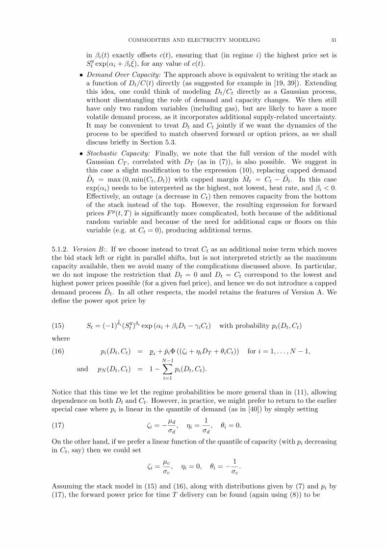
COMMODITIES AND ELECTRICITY MODELING 31
in βi(t) exactly offsets c(t), ensuring that (in regime i) the highest price set isSgt exp(αi + βiξ), for any value of c(t).
• Demand Over Capacity: The approach above is equivalent to writing the stack asa function of Dt/C(t) directly (as suggested for example in [19, 39]). Extendingthis idea, one could think of modeling Dt/Ct directly as a Gaussian process,without disentangling the role of demand and capacity changes. We then stillhave only two random variables (including gas), but are likely to have a morevolatile demand process, as it incorporates additional supply-related uncertainty.It may be convenient to treat Dt and Ct jointly if we want the dynamics of theprocess to be specified to match observed forward or option prices, as we shalldiscuss briefly in Section 5.3.
• Stochastic Capacity: Finally, we note that the full version of the model withGaussian CT , correlated with DT (as in (7)), is also possible. We suggest inthis case a slight modification to the expression (10), replacing capped demand
Dt = max (0,min(Ct, Dt)) with capped margin Mt = Ct − Dt. In this caseexp(αi) needs to be interpreted as the highest, not lowest, heat rate, and βi < 0.Effectively, an outage (a decrease in Ct) then removes capacity from the bottomof the stack instead of the top. However, the resulting expression for forwardprices F p(t, T ) is significantly more complicated, both because of the additionalrandom variable and because of the need for additional caps or floors on thisvariable (e.g. at Ct = 0), producing additional terms.
5.1.2. Version B:. If we choose instead to treat Ct as an additional noise term which movesthe bid stack left or right in parallel shifts, but is not interpreted strictly as the maximumcapacity available, then we avoid many of the complications discussed above. In particular,we do not impose the restriction that Dt = 0 and Dt = Ct correspond to the lowest andhighest power prices possible (for a given fuel price), and hence we do not introduce a capped
demand process Dt. In all other respects, the model retains the features of Version A. Wedefine the power spot price by
(15) St = (−1)δi(Sgt )δi exp (αi + βiDt − γiCt) with probability pi(Dt, Ct)
where
pi(Dt, Ct) = pi + piΦ ((ζi + ηiDT + θiCt)) for i = 1, . . . , N − 1,(16)
and pN (Dt, Ct) = 1−N−1∑i=1
pi(Dt, Ct).
Notice that this time we let the regime probabilities be more general than in (11), allowingdependence on both Dt and Ct. However, in practice, we might prefer to return to the earlierspecial case where pi is linear in the quantile of demand (as in [40]) by simply setting
(17) ζi = −µdσd, ηi =
1
σd, θi = 0.
On the other hand, if we prefer a linear function of the quantile of capacity (with pi decreasingin Ct, say) then we could set
ζi =µcσc, ηi = 0, θi = − 1
σc.
Assuming the stack model in (15) and (16), along with distributions given by (7) and pi by(17), the forward power price for time T delivery can be found (again using (8)) to be
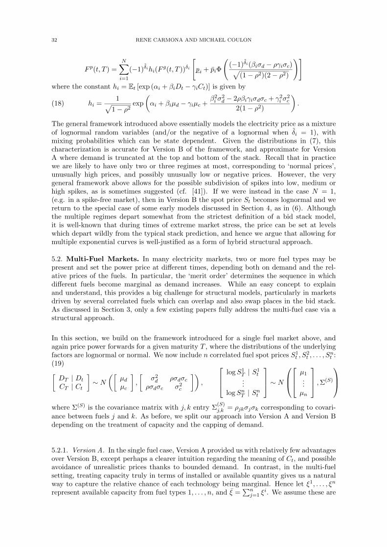
32 RENE CARMONA AND MICHAEL COULON
F p(t, T ) =
N∑i=1
(−1)δihi(Fg(t, T ))δi
[pi + piΦ
((−1)δi(βiσd − ργiσc)√
(1− ρ2)(2− ρ2)
)]where the constant hi = Et [exp (αi + βiDt − γiCt)] is given by
(18) hi =1√
1− ρ2exp
(αi + βiµd − γiµc +
β2i σ
2d − 2ρβiγiσdσc + γ2
i σ2c
2(1− ρ2)
).
The general framework introduced above essentially models the electricity price as a mixtureof lognormal random variables (and/or the negative of a lognormal when δi = 1), withmixing probabilities which can be state dependent. Given the distributions in (7), thischaracterization is accurate for Version B of the framework, and approximate for VersionA where demand is truncated at the top and bottom of the stack. Recall that in practicewe are likely to have only two or three regimes at most, corresponding to ‘normal prices’,unusually high prices, and possibly unusually low or negative prices. However, the verygeneral framework above allows for the possible subdivision of spikes into low, medium orhigh spikes, as is sometimes suggested (cf. [41]). If we were instead in the case N = 1,(e.g. in a spike-free market), then in Version B the spot price St becomes lognormal and wereturn to the special case of some early models discussed in Section 4, as in (6). Althoughthe multiple regimes depart somewhat from the strictest definition of a bid stack model,it is well-known that during times of extreme market stress, the price can be set at levelswhich depart wildly from the typical stack prediction, and hence we argue that allowing formultiple exponential curves is well-justified as a form of hybrid structural approach.
5.2. Multi-Fuel Markets. In many electricity markets, two or more fuel types may bepresent and set the power price at different times, depending both on demand and the rel-ative prices of the fuels. In particular, the ‘merit order’ determines the sequence in whichdifferent fuels become marginal as demand increases. While an easy concept to explainand understand, this provides a big challenge for structural models, particularly in marketsdriven by several correlated fuels which can overlap and also swap places in the bid stack.As discussed in Section 3, only a few existing papers fully address the multi-fuel case via astructural approach.
In this section, we build on the framework introduced for a single fuel market above, andagain price power forwards for a given maturity T , where the distributions of the underlyingfactors are lognormal or normal. We now include n correlated fuel spot prices S1
t , S2t , . . . , S
nt :
(19)[DT | Dt
CT | Ct
]∼ N
([µdµc
],
[σ2d ρσdσc
ρσdσc σ2c
]),
logS1T | S1
t...
logSnT | Snt
∼ N µ1
...µn
,Σ(S)
where Σ(S) is the covariance matrix with j, k entry Σ
(S)j,k = ρjkσjσk corresponding to covari-
ance between fuels j and k. As before, we split our approach into Version A and Version Bdepending on the treatment of capacity and the capping of demand.
5.2.1. Version A. In the single fuel case, Version A provided us with relatively few advantagesover Version B, except perhaps a clearer intuition regarding the meaning of Ct, and possibleavoidance of unrealistic prices thanks to bounded demand. In contrast, in the multi-fuelsetting, treating capacity truly in terms of installed or available quantity gives us a naturalway to capture the relative chance of each technology being marginal. Hence let ξ1, . . . , ξn
represent available capacity from fuel types 1, . . . , n, and ξ =∑n
j=1 ξi. We assume these are
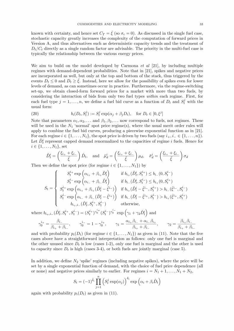
COMMODITIES AND ELECTRICITY MODELING 33
known with certainty, and hence set CT = ξ (so σc = 0). As discussed in the single fuel case,stochastic capacity greatly increases the complexity of the computation of forward prices inVersion A, and thus alternatives such as deterministic capacity trends and the treatment ofDt/Ct directly as a single random factor are advisable. The priority in the multi-fuel case istypically the relationship between the various energy prices.
We aim to build on the model developed by Carmona et al [21], by including multipleregimes with demand-dependent probabilities. Note that in [21], spikes and negative pricesare incorporated as well, but only at the top and bottom of the stack, thus triggered by theevents Dt ≤ 0 and Dt ≥ ξ. Instead, here we allow for the possibility of spikes even for lowerlevels of demand, as can sometimes occur in practice. Furthermore, via the regime-switchingset-up, we obtain closed-form forward prices for a market with more than two fuels, byconsidering the interaction of bids from only two fuel types within each regime. First, for
each fuel type j = 1, . . . , n, we define a fuel bid curve as a function of Dt and Sjt with theusual form:
(20) bi(Dt, Sjt ) := Sjt exp(αj + βjDt), for Dt ∈ [0, ξj ]
Note that parameters α1, α2, . . . and β1, β2, . . . now correspond to fuels, not regimes. Thesewill be used in the N1 ‘normal’ spot price regime(s), where the usual merit order rules willapply to combine the fuel bid curves, producing a piecewise exponential function as in [21].For each regime i ∈ {1, . . . , N1}, the spot price is driven by two fuels (say i+, i− ∈ {1, . . . , n}).Let Di
t represent capped demand renormalized to the capacities of regime i fuels. Hence fori ∈ {1, . . . , N1}, set
Dit =
(ξi+ + ξi−
ξ
)Dt, and µid =
(ξi+ + ξi−
ξ
)µd, σid =
(ξi+ + ξi−
ξ
)σd
Then we define the spot price (for regime i ∈ {1, . . . , N1}) by
St =
Si+t exp
(αi+ + βi+D
it
)if bi+(Di
t, Si+t ) ≤ bi−(0, S
i−t )
Si−t exp
(αi− + βi−D
it
)if bi−(Di
t, Si−t ) ≤ bi+(0, S
i+t )
Si+t exp
(αi+ + βi+(Di
t − ξi−))
if bi+(Dit − ξi− , S
i+t ) > bi−(ξi− , S
i−t )
Si−t exp
(αi− + βi−(Di
t − ξi+))
if bi−(Dit − ξi+ , S
i−t ) > bi+(ξi+ , S
i+t )
bi+,i−(Dit, S
i+t , S
i−t ) otherwise,
where bi+,i−(Dit, S
i+t , S
i−t ) = (S
i+t )γ
i+0 (S
i−t )γ
i−0 exp
(γ1 + γ2D
it
)and
γi+0 =
βi−βi+ + βi−
, γi−0 = 1− γi+0 , γ1 =
αi+βi− + αi−βi+βi+ + βi−
, γ2 =βi+βi−βi+ + βi−
and with probability pi(Dt) (for regime i ∈ {1, . . . , N1}) as given in (11). Note that the fivecases above have a straightforward interpretation as follows: only one fuel is marginal andthe other unused since Dt is low (cases 1-2), only one fuel is marginal and the other is usedto capacity since Dt is high (cases 3-4), or both fuels are jointly marginal (case 5).
In addition, we define N2 ‘spike’ regimes (including negative spikes), where the price will beset by a single exponential function of demand, with the choice of fuel price dependence (allor none) and negative prices similarly to earlier. For regimes i = N1 + 1, . . . , N1 +N2,
St = (−1)δin∏j=1
(Sjt exp(αj)
)δiexp
(αi + βiDt
)again with probability pi(Dt) as given in (11).
34 RENE CARMONA AND MICHAEL COULON
We let Ji = {i+, i−} represent the set of two fuels (with prices SJit = (Si+t , S
i−t )) driving
power prices in ‘normal’ regime i, for i ∈ {1, . . . , N1} and hence use notation bJi(Dt,SJit )
for the case of jointly margin fuels (case 5 above). Without loss of generality, we assign i+and i− such that ξi+ ≥ ξi− . Finally, as all terms have approximately the same form, weintroduce one more piece of useful notation:
Φpi3
([x1
x2
], y, z; ρ
):= piΦ2
([x1
x2
], y; ρ
)+ pi
(Φ3(x1, y, z2; Σ)− Φ3(x2, y, z2; Σ)
)where
Σ =
1 ρ −1/√
2
ρ 1 −ρ/√
2
−1/√
2 −ρ/√
2 1
.
Then (using (9)) the forward power price F pt for time T delivery can be written as followsin terms of the forward fuel prices F 1
t , . . . , Fnt (notation shortened for convenience):
F pt =
N1∑i=1
∑j∈Ji
eβ2j (σ
id)
2
2
bj (µid, F jt )Φpi3
ξj−µidσid− βj σid
−µidσid− βj σid
, Rjk(µid, 0)− β2j (σid)
2
σj,d,βj σ
id√
2;βj σ
id
σj,d
+bj
(µid − ξk, F
jt
)Φpi
3
ξ−µidσid− βj σid
ξk−µidσid− βj σid
, −Rjk(µid − ξk, ξk
)+ β2
j (σid)2
σj,d,βj σ
id√
2;−βj σidσj,d
+∑j∈Ji
δjeηbJi(µ
id,F
Jit )
−Φpi3
ξj−µidσid− γ2σ
id
−µidσid− γ2σ
id
, Rjk(µid, 0) + γk0σ2 − γ2βj(σ
id)
2
δjσj,d,γ2σ
id√
2;βj σ
id
δjσj,d
+ Φpi
3
ξ−µidσid− γ2σ
id
ξk−µidσid− γ2σ
id
, Rjk(µid − ξk, ξk
)+ γk0σ
2 − γ2βj(σid)
2
δjσj,d,γ2σ
id√
2;βj σ
id
δjσj,d
+
[piΦ
(−µidσid
)+ piΦ2
(−µidσid
, 0;−1√
2
)]∑j∈Ji
bj
(0, F jt
)Φ
(Rjk(0, 0)
σJi
)
+
[piΦ
(µid − ξσid
)+ piΦ2
(µid − ξσid
, 0;−1√
2
)]∑i∈I
bj
(ξj , F jt
)Φ
−Rjk(ξj , ξk
)σJi
+
N2∑i=N1+1
(−1)δi
n∏j=1
F jt
δi
exp
δi n∑j=1
(αj −
1
2σ2j +
n∑k=1
Σ(S)j,k
) f(µd, σd, ξ, pi, pi, αi, βi, δi)
where k = Ji \ {j}, δj = (−1)I{j=i+} (for j ∈ Ji, where i ∈ {1, . . . N1}), with f(·) as defined
in (14) and
σ2Ji := σ2
i+ − 2ρi+i−σi+σi− + σ2i− ,
σ2j,d := β2
j (σid)2 + σ2
Ji ,
η :=γ2
2(σid)2 − αcαgσ2
2
Rjk (ξj , ξk) := αk + βkξk − αj − βjξj + log(F kt
)− log
(F jt
)− 1
2σ2Ji .
Although the formula above appears remarkably involved, note that for a two fuel market(e.g. gas and coal) we are likely to only have one ‘normal’ regime (N1 = 1) and one or twoother regimes, reducing the complexity of the formula. If N2 = 0, we return to the resultof [21]. However, the additional generality allows extra flexibility. For example, in a market
COMMODITIES AND ELECTRICITY MODELING 35
with three fuels but very little chance of overlap between the highest and lowest, we mightset N1 = 2, prescribing one regime where the highest fuel mixes with the middle fuel, andone where the middle fuel mixes with the lowest.
5.2.2. Version B. In the second version of the multi-fuel framework, we do not define ca-pacities ξ1, . . . , ξn. Hence it is less clear how to capture changes in the merit order, becausethere is no concept of a threshold capacity level where the marginal fuel type changes whendemand crosses that threshold. Instead, the only way to approximate the subtle interplaybetween demand and marginal fuel type is to use the idea of regimes instead. For example,for an n fuel market, one might define n+1 regimes, one driven by each underlying fuel, andone for spikes. Although this does not incorporate an overlap regime, the simplification toa single marginal fuel is intuitively appealing and similar in spirit to the work of Aıd et al[1, 2]. Instead of their strict capacity-driven thresholds, we then use our demand-dependentregime probabilities to ensure that fuels higher in the merit order are more likely to beused when demand is high. A big obstacle to either approach is that the merit order maychange, particularly over medium to long time horizons. Indeed, in [2], to retain mathemat-ical tractability in the n fuel case, the authors assume that the initial merit order is fixedand enforce this by modeling the spreads between neighbouring fuels as Geometric BrownianMotions, a departure from commonly-used models for fuel prices. In this section, we presentanother variation in order to retain the chance of future merit order changes, following moreclosely the original setup of [1].
Similarly to (20), we define an exponential curve for each fuel type, but now treating Ct asan additional stochastic factor
bi(Dt, Ct, Sit) := Sit exp(αi + βiDt − γiCt), for i = 1, . . . , n.
Regimes 1, . . . , n (the ‘normal’ regimes) will be driven by fuels 1, . . . , n only. Note that it iscertainly possible to incorporate ‘overlap’ regimes in this framework, for example by choosingthe function (S1
t )ε(S2t )1−ε exp(α1,2 + β1,2Dt − γ1,2Ct) for a regime driven jointly by fuels 1
and 2. While explicit forward curves can still be found, this adds unnecessary complicationsfor our illustrative purposes here. Regimes n+ 1, . . . , N (the ‘spike’ regimes) will be drivenby either no fuels or all fuels jointly. Thus,
bi(Dt, Ct, Sit) := (−1)δi
n∏j=1
(Sjt exp(αj)
)δiexp (αi + βiDt − γiCt) for i = n+ 1, . . . , N
Next, before defining the power price St, we define a permutation {πt(1), . . . , πt(n)} over theset {1, . . . , n} of fuels, such that
Sπt(1)t exp(απt(1) + βπt(1)µd) ≥ . . . ≥ S
πt(n)t exp(απt(n) + βπt(n)µd).
This is similar to the approach followed in [1], but without the restriction of a single heatrate per fuel type (i.e. a step function bid stack). We then define the spot price as
(21) St = bπt(i)(Dt, Ct, Sπt(i)t ) with probability pi(Dt, Ct)
where again (in the most general form)
pi(Dt, Ct) = pi + piΦ ((ζi + ηiDt + θiCt)) for i = 1, . . . , N − 1,
and pN (Dt, Ct) = 1−N−1∑i=1
pi(Dt, Ct).
In other words, the idea is that πt approximately captures the ordering of fuel types (themerit order), using the average demand level in the market. Then the regime probabilitiespi (increasing in Dt for lower values of i, decreasing in Dt for higher values of i) can do
36 RENE CARMONA AND MICHAEL COULON
the work of linking the more expensive fuel types to higher demand states, and the cheaperones to lower demand states. Unlike in Version A, determining which fuel price sets thepower prices does not depend on a function of both Dt and S1
t , . . . , Snt jointly, thus easing
the computation of forward prices. While the connection between demand and price is looserthan in a strict stack model, this is not necessarily unrealistic for a market with significantnoise from Ct.
Assuming the model in (21), distributions in (19) and pi given by (17) for simplicity, in thecase of two fuels (n = 2) the forward power price F pt for time T delivery is given by
F pt =
2∑i=1
2∑j=1
hjFjt Φ
((−1)iRjk(µd, µd)√σ2
1 − 2ρ12σ1σ2 + σ22
)[pi + piΦ
((βjσd − ργjσc)√(1− ρ2)(2− ρ2)
)]+
N∑i=3
(−1)δihi
F 1t F
2t exp
2ρ12σ1σ2 +2∑j=1
(αj +1
2σ2j )
δi [pi + piΦ
((−1)δi(βiσd − ργiσc)√
(1− ρ2)(2− ρ2)
)]where k = {1, 2}\j and as before, hi = Et [exp (αi + βiDt − γiCt)] as given (for i = 1, . . . , N)in (18) and Rjk also as defined earlier.
At the expense of a weaker link to the merit order, this result is clearly much simpler thanthe Version A forward price, due to the lack of any indicator functions involving demand.Nonetheless the complexity increases rapidly for more than two fuels. The three fuel case(n = 3) is still realistic to write out on paper (using the trivariate relationship in (9) and somedetermination!), but for n > 3 the increasing dimensionality of the multivariate Gaussianand the increasing number of permutations of fuels renders a closed-form solution nearlyinfeasible, although numerical implementation is still straightforward.
5.3. Parameter Estimation and Forward Curve Calibration. The choice of structuralmodel clearly depends on both the electricity market in question and the goals of the model.The framework above and its many versions were intended to emphasize the variety of toolsavailable for modeling the many features we observe in price dynamics, while retaining acommon core to the model and a reasonable level of mathematical tractability. No matterwhich specific model is ultimately chosen, an important next step is a reliable and robustmethod for parameter estimation and forward curve calibration. These two issues are mostoften tackled in stages, first estimating some parameters from history, and then selectingothers to match forward looking market quotes. In all cases, the explicit formulas above forF p(t, T ) (and their explicit dependence on fuel forwards) provide a valuable computationalbenefit, as an optimal fit to observed forward curves in a high dimensional model quicklybecomes unmanageable if limited to Monte Carlo simulation. In this subsection we discussbriefly the main challenges involved in fitting a structural model to data.
• Observable vs Unobservable Factors: As discussed throughout this paper, manyof the underlying factors (e.g. demand, fuel prices) in electricity markets are eas-ily observable and exogenously modelled, meaning that their parameters can beestimated independently of the power price model itself, by standard techniquessuch as maximum likelihood. However, the sheer complexity of the market typ-ically means that some factors are either truly unobservable or their treatmentin the model approximates several effects, making them effectively unobservablefor modeling purposes. In our framework, ‘capacity’ Ct typically falls in this cat-egory, particularly when treated as a catch-all noise process (i.e. Version B). Insuch cases the model-implied history of the process can be backed out from spotprice histories as a model residual (as suggested in [72, 68, 39] among others),
COMMODITIES AND ELECTRICITY MODELING 37
typically producing a closer fit to historical price dynamics. However this benefitmust be weighed against the risk that structural or regulatory changes can makemarket price histories unreliable, a weakness not suffered by models driven onlyby observed factors.
• Stack Parameters: As discussed by [68] and [49] among others, the estimationof stack parameters (α’s and β’s in our expressions) can be achieved in severalways. In summary, (i) from costs, (ii) from bids, (iii) from prices. The first of theserelies somewhat on the assumption of competitive markets and limited strategybidding (ie, generators bidding their production costs), but has the significantadvantage of avoiding messy estimation and fixing some key parameters to wellunderstood market variables. For example, in the multi-fuel case (Version A),we may be able to easily approximate the range of heat rates (efficiencies) in themarket for each technology j ∈ {1, . . . , n}, which can then be equated to the range[exp(αj), exp(αj+βjξ
j)] for the ‘normal’ regimes. On the other hand, if historicalauction data is available, then parameters α and β can be fitted directly to the bidstack (as in [39]), though this is less suitable if there are multiple ‘normal’ regimes.Finally, the use of only prices to fit the exponential bid curves is disadvantageoussince we only observe one point on the curve each hour. Hence regions of thecurves which only rarely set the price may be harder to accurately estimate thanwhen using the historical stack data. However, as the occurrence of ‘spike’ regimesin history is unobservable, price data may be particularly useful for filtering outthese extreme points, and fitting their parameters separately. In practice, goodjudgement is needed from market to market when deciding how best to tacklestack calibration, and a combination of the above options may be preferable.
• History vs Market Quotes: The choice between using history and using currentmarket quotes revolves around several key questions, including the availability andreliability of data, the treatment of risk premia, and the desired model inputs.Variables such as temperature (which can be mapped to demand, as discussed inSection 3.2) have long and reliable histories, and are hence one of the argumentsin favor of structural models over reduced-form. However, fitting all parametersto history and assuming a constant market price of risk when needed will of coursefail to reproduce the market forward prices, a typical first step in any modelingproblem. Therefore, a balance must be struck between parameters matched tohistory and parameters matched to future risk-neutral dynamics (i.e. to observedprices). The simplest approach in the structural framework described above is tofirst fit everything to history, before allowing the mean level of demand µd (orcapacity µc) to be time-dependent, chosen precisely to reproduce each marketforward price F p(t, T ) (see, [37] for a similar approach in reduced-form). Solvingfor µd numerically is straightforward given the expressions above, giving an exactcalibration to the forward curve. In other cases, we may be interested in allowingmore parameters to be free, in order to match other input prices from the market,such as at-the-money options if they are sufficiently liquid.
• Risk premia: A key advantage of the expressions above is that power forwardsF p(t, T ) are written directly in terms of fuel forwards (say F g(t, T )), which can betreated as observed market prices. Hence, for the fuel component of our model, noassumption regarding risk premia is needed, as the risk-neutral drift is implicitlyspecified by observed forwards. Moreover, no calibration technique is needed forthe fuel forward curves. On the other hand, the dynamics of other factors suchas demand and capacity can only be estimated under the physical measure viahistory (unless the careful use of weather derivatives can provide information fordemand via temperature). Hence, rather arbitrary assumptions about the form
38 RENE CARMONA AND MICHAEL COULON
of the market price(s) of risk may be required. However, as discussed in theprevious paragraph, we typically desire exact calibration to the observed powerforward curve, through which the market price of risk can be absorbed into themean level µd (or µc) needed to match forwards. While this may simply sweepthe issue under the carpet, for many practical applications it should suffice as areasonable assumption and claims of incompleteness can be politely ignored bypointing to a liquid forward curve for all maturities.
• Delivery Periods: As we gently sweep one issue under the carpet, another crops uparound the corner! While it may be true that liquid forward prices exist coveringseveral years from the current time, they certainly do not exist for every specificmaturity T , simply because of delivery periods. As mentioned in Section 2, theconvention in all electricity markets is that forward contracts specify electricitydelivery over a period of time, often one month, but sometimes even a quarteror a year for longer contracts. Hence the price should be written F (t, T1, T2) andcorrespond to an average of the expected spot price for all hours in the month (ordelivery period). While some authors have approximated this in continuous timeas an integral over the delivery period and designed models for which the integralsimplifies (cf. [13, 11]), in reality a sum is arguably more appropriate, since Stis indeed a discrete time process. Adding an outer summation to our expressionsabove is a simple adjustment, but in this case we should note that fuel forwardprices then also require single hour maturities, which is unfortunately not thecase, as these are typically also monthly. Various remedies are possible, includingthe smoothing of observed forward curves to obtain prices for all T (cf. [12, 61]for smoothing electricity forward quotes), the assumption of piecewise constantfuel forwards, or the choice of a representative single date per delivery period(reasonable for longer maturities). Unfortunately, there is no clear answer, andsuch implementation challenges exist no matter what price model we use!
• Hour of Day Considerations: Finally, we note that observed power forward curvesoften exist for delivery over different hours of the day (day vs. night) and days ofthe week (weekday vs. weekend), categorized as peak, off-peak or base-load con-tracts. Hence, the calibration to observed forward quotes may require multiplecalibrations per delivery month. In the simplest case, one might simply adjustthe mean demand µd (or µc) by a different amount for peak and off-peak hours.A well-fitted model for load should first capture the well-known hourly patternsacross the day, as well as seasonal periodicities which may vary significantly fordifferent hours of the day. While some authors have chosen to treat each hourof the day as a separate (but correlated) stochastic process, others treat only thedeterministic component of demand differently by hour. Having 24 separate pro-cesses may introduce too many parameters, particularly as the historical samplesize drops significantly, making it hard for example to stably model the tail of theprice distribution.
In conclusion, the fitting procedure for structural models is typically a fine art, combiningdifferent approaches for different components of the overall framework. As with all modelsfor electricity, approximations must be made. Structural models in particular may have verymany parameters to estimate, but in exchange can have much data available to help.
6. Conclusion
In this survey, we have attempted to give the reader a flavour of many of the interestingand unique characteristics of energy (and commodity) markets, and in particular the mostunusual of all, electricity. While many different price modeling approaches now exist, the
COMMODITIES AND ELECTRICITY MODELING 39
topic still provides many avenues for important new research, both building on current workand addressing new questions as they arise. For example, how will electricity grids managethe rapid growth of renewable energy with large supply variability, and how will prices beaffected? Will the emissions markets grow in importance globally and produce more dramaticchanges in the merit order? Will the smart grid and growth of electric vehicles cause astructural change, with both the demand inelasticity and non-storability assumptions underthreat? Will new storage technology bring electricity price dynamics closer in line with othercommodities? What about the ‘financialization’ of electricity, if power forwards some daybegin to appear in commodity indices? How global can electricity markets become (e.g. withsolar panels in the Sahara powering much of Europe and Africa)? Some of these thoughtsmay be a long way off, but others could be just around the corner! We do not promotethe structural approach discussed in detail here as an answer to such intriguing speculativequestions, but we do recommend thinking beyond the historical price series, especially attimes of fundamental market change. We have presented and discussed structural modelswhich meet this criteria by directly incorporating demand, capacity and fuel prices, andwithout necessarily sacrificing the mathematical benefits traditionally reserved for reduced-form approaches. We hope that the flexible, intuitive and practical framework we advocatecan play a useful role in understanding and tackling the many risks ahead in the fascinatingnext chapter of the global energy markets.
References
[1] R. Aıd, L. Campi, Adrien N. Huu, and N. Touzi. A structural risk-neutral model of electricity prices.International Journal of Theoretical and Applied Finance, 12:925–947, 2009.
[2] R. Aıd, L. Campi, and N. Langrene. A structural risk-neutral model for pricing and hedging powerderivatives. Mathematical Finance. Published on Line Feb. 13, 2012.
[3] R. Aıd, A. Chemla, A. Porchet, and N. Touzi. Hedging and vertical integration in electricity markets.Management Science, 57:1438–1452, 2011.
[4] C.L. Anderson and M. Davison. A hybrid system-econometric model for electricity spot prices: Consid-ering spike sensitivity to forced outage distributions. IEEE Transactions on Power Systems, 23:927–937,2008.
[5] N. Audet, P. Heiskanen, J. Keppo, and I. Vehvilainen. Modeling electricity forward curve dynamics in thenordic market. In D. Bunn, editor, Modelling Prices in Competitive Electricity Markets, pages 251–265.Wiley, 2004.
[6] E. Banks. Weather Risk Management: Markets, Products and Applications. Palgrave, 2002.[7] M. Barlow. A diffusion model for electricity prices. Mathematical Finance, 12(4):287–298, 2002.[8] O.E. Barndorff-Nielsen, F.E. Benth, and A.E.D. Veraart. Modelling electricity forward prices by ambit
fields. Technical report, 2011. Preprint.[9] O.E. Barndorff-Nielsen, F.E. Benth, and A.E.D. Veraart. Modelling energy spot prices by Levy semista-
tionary processes. Technical report, 2011. Preprint.[10] P. Barrieu and N. El Karoui. Pricing, hedging and designing derivatives with risk measures. In R. Car-
mona, editor, Indifference Pricing, pages 77–146. Princeton University Press, Princeton, NJ, 2009.[11] F. E. Benth, J. Kallsen, and T. Meyer-Brandis. A non-gaussian ornstein-uhlenbeck process for electricity
spot price modeling and derivatives pricing. Applied Mathematical Finance, 14:153–169, 2007.[12] F. E. Benth, S. Koekebakker, and F. Ollmar. Extracting and applying smooth forward curves from
average-based commodity contracts with seasonal variation. Journal of Derivatives, Fall 15:52–66, 2007.[13] F.E. Benth, J.S. Benth, and S. Koekebakker. Stochastic Modeling of Electricity and Related Markets.
World Scientific.[14] M. Bernhart, H. Pham, P. Tankov, and X. Warin. Swing options valuation: A bsde with constrained
jumps approach. In R. Carmona et al., editor, Numerical methods in finance, Springer Proceedings inMathematics. Springer Verlag, 2012.
[15] T. Bjork and C. Landen. On the term structure of futures and forward prices. In Eds.), MathematicalFinance-Bachelier Congress 2000, pages 111–149. Springer, 2002.
[16] A. Boogert and D. Dupont. When supply meets demand: the case of hourly spot electricity prices. IEEETransactions on Power Systems, 23(2):389–398, 2008.
[17] I. Bouchouev. The inconvenience yield or the theory of normal contango. Energy Risk Magazine, Sep-tember 2011.
[18] M. Burger, B. Graeber, and G. Schindlmayr. Managing Energy Risk: An Integrated View on Power andOther Energy Markets. Wiley.
40 RENE CARMONA AND MICHAEL COULON
[19] M. Burger, B. Klar, A. Muller, and G. Schindlmayr. A spot market model for pricing derivatives inelectricity markets. Quantitative Finance, 4:109–122, 2004.
[20] R. Carmona. Applications to weather derivatives and energy contracts. In R. Carmona, editor, Indiffer-ence Pricing, pages 241–264. Princeton University Press, Princeton, NJ, 2009.
[21] R. Carmona, M. Coulon, and D. Schwarz. Electricity price modeling and asset valuation: a multi-fuelstructural approach. Technical report, 2012.
[22] R. Carmona, M. Coulon, and D. Schwarz. The valuation of clean spark spread options: Linking electricity,emissions and fuels. Technical report, 2012.
[23] R. Carmona and S. Dayanik. Optimal multiple stopping of linear diffusions. Mathematics of OperationsResearch, 33:446–460, 2008.
[24] R. Carmona and P. Diko. Pricing precipitation based derivatives. International Journal of Theoreticaland Applied Finance, 7:959–988, 2005.
[25] R. Carmona and V. Durrleman. Pricing and hedging spread options. SIAM Rev., 45(4):627–685, 2003.[26] R. Carmona, F. Fehr, J. Hinz, and A. Porchet. Market designs for emissions trading schemes. SIAM
Review, 52:403–452, 2010.[27] R. Carmona and J. Hinz. Least Squares Monte Carlo approach to convex control problems. Technical
report, Princeton University, 2011.[28] R. Carmona and M. Ludkovski. Valuation of energy storage: an optimal switching approach. Quantitative
Finance, pages 359–374.[29] R. Carmona and M. Ludkovski. Spot convenience yield models for the energy markets. In Mathematics
of finance, volume 351 of Contemp. Math., pages 65–79. Amer. Math. Soc., Providence, RI, 2004.[30] R. Carmona and M. Ludkovski. Pricing asset scheduling flexibility using optimal switching. Applied
Mathematical Finance, 15(5):405–447, 2008.[31] R. Carmona and Y. Sun. Implied and local correlations from spread options. Applied Mathematical
Finance, 2012. (to appear).[32] R. Carmona and N. Touzi. Optimal multiple stopping and valuation of swing options, 2008.[33] P. Carr and D. Madan. Option valuation using the fast Fourier transform. Journal of Computational
Finance, 2(5):61 – 73, 1998.[34] A. Cartea and M. Figueroa. Pricing in electricity markets: A mean reverting jump diffusion model with
seasonality. Applied Mathematical Finance, 12(4):313–335.[35] A. Cartea, M. Figueroa, and H. Geman. Modelling electricity prices with forward looking capacity
constraints. Applied Mathematical Finance, 32:2501–2519, 2008.[36] A. Cartea and P. Villaplana. Spot price modeling and the valuation of electricity forward contracts: the
role of demand and capacity. Journal of Banking and Finance, 32:2501–2519, 2008.[37] L. Clewlow and C. Strickland. Valuing energy options in a one factor model fitted to forward prices.
working paper, 1999.[38] L. Clewlow and C. Strickland. Energy Derivatives: Pricing and Risk Management. Lacima Productions,
2000.[39] M. Coulon and S. Howison. Stochastic behaviour of the electricity bid stack: from fundamental drivers
to power prices. Journal of Energy Markets, 2:29–69, 2009.[40] M. Coulon, W. Powell, and R. Sircar. A model for hedging load and price risk in the Texas electricity
market. Technical report, 2012.[41] M. Culot, V. Goffin, S. Lawford, S. de Menten, and Y. Smeers. An affine jump diffusion model for
electricity. working paper, Catholic University of Leuven.[42] G.d.M. D’Aertrycke and Y. Smeers. The valuation of power futures based on optimal dispatch. Journal
of Energy Markets, 3(3):27–50, 2010.[43] C. De Jong and R. Huisman. Option pricing for power prices with spikes. Energy Power Risk Management,
7:12–16, 2003.[44] C. De Jong and S. Schneider. Cointegration between gas and power spot prices. Journal of Energy
Markets, 2(3):27–46, 2009.[45] S. Deng. Stochastic models of energy commodity prices and their applications: Mean-reversion with
jumps and spikes. Technical report, University of California Energy Institute, 1999.[46] D. Duffie, J. Pan, and K. Singleton. Transform analysis and asset pricing for affine jump-diffusions.
Econometrica, 68(6):1343–76, 2000.[47] G. W. Emery and Q. Liu. An analysis of the relationship between electricity and natural-gas futures
prices. The Journal of Futures Markets, 22(2):95–122, 2002.[48] A. Eydeland and H. Geman. Pricing power derivatives. Risk Magazine, 10:71–73, 1998.[49] A. Eydeland and K. Wolyniec. Energy and Power Risk Management: New Developments in Modeling,
Pricing and Hedging. Finance. Wiley, 2003.[50] P. Forsythe. A semi-lagrangian approach for natural gas valuation and optimal operation. SIAM Journal
on Scientific Computing, 30:339–368, 2007.
COMMODITIES AND ELECTRICITY MODELING 41
[51] N. Frikha and V. Lemaire. Joint modelling of gas and electricity spot prices. Applied MathematicalFinance, 2012. to appear.
[52] H. Geman. Commodities and commodity derivatives: Modeling and Pricing of Agriculturals, Metals andEnergy. Finance. Wiley, 2005.
[53] H. Geman. Risk Management in Commodity Markets: From Shipping to Agriculturals and Energy. Fi-nance. Wiley, 2008.
[54] H. Geman and A. Roncoroni. Understanding the fine structure of electricity prices. Journal of Business,79, 2006.
[55] R. Gibson and E. S. Schwartz. Stochastic convenience yield and the pricing of oil contingent claims.Journal of Finance, XLV(3):959–976, 1990.
[56] S. Howison and D. Schwarz. Structural modelling of carbon emission markets. Technical report, 2012.submitted.
[57] P. Jaillet, E. Ronn, and S. Tompaidis. Valuation of commodity-based swing options. Management Science,50:909921, 2004.
[58] S. Jaimungal and V. Surkov. Levy based cross-commodity models and derivative valuation. SIAM Journalof Financial Mathematics, 2:464 –, 2011.
[59] T. Kanamura and K. Ohashi. A structural model for electricity prices with spikes: measurement of spikerisk and optimal policies for hydropower plant operation. Energy Economics, 29(5):1010–1032, 2007.
[60] V. Kholodnyi. A non-markovian process for power prices with spikes and valuation of european contigentclaims on power. Technical report, Erasmus Energy Library, 2001.
[61] T. Kluge. Pricing Swing Options and Other Electricity Derivatives. PhD thesis, 2006. DPhil Thesis,University of Oxford.
[62] S. Koekebakker and F. Ollmar. Forward curve dynamics in the nordic electricity market. ManagerialFinance, 31:74–95, 2005.
[63] R. Litterman and J. Scheinkman. Common factors affecting bond returns. Journal of Fixed Income,1:49–53, 1991.
[64] J. Lucia and E. Schwartz. Electricity prices and power derivatives: Evidence from the nordic powerexchange. Review of Derivatives Research, 2002.
[65] M. Lyle and R. Elliott. A ”simple” hybrid model for power derivatives. Energy Economics, 31:757–767,2009.
[66] T.D. Mount, Y. Ning, and X. Cai. Predicting price spikes in electricity markets using a regime-switchingmodel with time-varying parameters. Energy Economics, 28:62–80, 2006.
[67] C. Pirrong. Commodity Price Dynamics: A Structural Approach. Cambridge University Press, 2012.[68] C. Pirrong and M. Jermakyan. The price of power: The valuation of power and weather derivatives.
Journal of Banking and Finance, 32:2520–2529, 2008.[69] J. Porter. Evolution of the global weather derivatives market. In P. Field, editor, Modern Risk Manage-
ment: a History. Risk Books, 2004.[70] E. Schwartz. The stochastic behaviour of commodity prices: Implications for valuation and hedging. The
Journal of Finance, 3:923–973, 1997.[71] E. Schwartz and J. Smith. Short-term variations and long-term dynamics in commodity prices. Manage-
ment Science, 46:893–911, 2000.[72] P. Skantze, A. Gubina, and M. Ilic. Bid-based stochastic model for electricity prices: the impact of
fundamental drivers on market dynamics. MIT E-lab report, November 2000.[73] K. Tang and W. Xiong. Index investment and financialization of commodities. Technical report, 2010.
NBER Working Paper 16385.[74] S. Thoenes. Understanding the determinants of electricity prices and the impact of the German Nuclear
Moratorium in 2011. Technical report, 2011. EWI Working Paper.[75] F. Turboult and Y. Youlal. Swing option pricing by optimal exercise boundary estimation. In R. Carmona
et al., editor, Numerical methods in finance, Springer Proceedings in Mathematics. Springer Verlag, 2012.[76] A. Wagner. Residual demand modelling and application to electricity pricing. Technical report, Technis-
che Universitaet Kaiserslautern, 2012.[77] X. Warin. Gas storage hedging. In R. Carmona et al., editor, Numerical methods in finance, Springer
Proceedings in Mathematics. Springer Verlag, 2012.[78] R. Weron. Modeling and and Forecasting Electricity Loads and Prices: a statistical approach. Wiley.[79] R. Weron, M. Bierbrauer, and S. Truck. Modeling electricity prices: jump diffusion and regime switching.
Physica A: Statistical Methods and It’s Applications, 336:39–48, 2004.[80] K. Wiebauer. A practical view on valuation of multi-exercise american style options in gas and elec-
tricitymarkets. In R. Carmona et al., editor, Numerical methods in finance, Springer Proceedings inMathematics. Springer Verlag, 2012.

42 RENE CARMONA AND MICHAEL COULON
Bendheim Center for Finance, Dept. ORFE, Princeton University, Princeton NJ 08544, USA
E-mail address: [email protected]
ORFE, University of Princeton, Princeton NJ 08544, USA
E-mail address: [email protected]
Related Documents