A Support Vector Machine-Based Dynamic Network for Visual Speech Recognition Applications

EURASIP Journal on Applied Signal Processing 2002:11, 1248–1259c© 2002 Hindawi Publishing Corporation

A Support Vector Machine-Based Dynamic Networkfor Visual Speech Recognition Applications

Mihaela GordanDepartment of Informatics, Aristotle University of Thessaloniki, Box 451, Thessaloniki 54006, GreeceEmail: [email protected]

Constantine KotropoulosDepartment of Informatics, Aristotle University of Thessaloniki, Box 451, Thessaloniki 54006, GreeceEmail: [email protected]

Ioannis PitasDepartment of Informatics, Aristotle University of Thessaloniki, Box 451, Thessaloniki 54006, GreeceEmail: [email protected]

Received 26 November 2001 and in revised form 26 July 2002

Visual speech recognition is an emerging research field. In this paper, we examine the suitability of support vector machines forvisual speech recognition. Each word is modeled as a temporal sequence of visemes corresponding to the different phones realized.One support vector machine is trained to recognize each viseme and its output is converted to a posterior probability through asigmoidal mapping. To model the temporal character of speech, the support vector machines are integrated as nodes into a Viterbilattice. We test the performance of the proposed approach on a small visual speech recognition task, namely the recognition of thefirst four digits in English. The word recognition rate obtained is at the level of the previous best reported rates.

Keywords and phrases: visual speech recognition, mouth shape recognition, visemes, phonemes, support vector machines, Viterbilattice.

1. INTRODUCTION

Audio-visual speech recognition is an emerging research fieldwhere multimodal signal processing is required. The motiva-tion for using the visual information in performing speechrecognition lays on the fact that the human speech produc-tion is bimodal by its nature. In particular, human speechis produced by the vibration of the vocal cords and dependson the configuration of the articulatory organs, such as thenasal cavity, the tongue, the teeth, the velum, and the lips. Aspeaker produces speech using these articulatory organs to-gether with the muscles that generate facial expressions. Be-cause some of the articulators, such as the tongue, the teeth,and the lips are visible, there is an inherent relationship be-tween the acoustic and visible speech. As a consequence, thespeech can be partially recognized from the information ofthe visible articulators involved in its production and in par-ticular from the image region comprising the mouth [1, 2, 3].

Undoubtedly, the most useful information for speechrecognition is carried by the acoustic signal. When the acous-tic speech is clean, performing visual speech recognition andintegrating the recognition results from both modalities does

not bring too much improvement because the recognitionrate from the acoustic information alone is very high, if notperfect. However, when the acoustic speech is degraded bynoise, adding the visual information to the acoustic one im-proves significantly the recognition rate. Under noisy con-ditions, it has been proved that the use of both modalitiesfor speech recognition is equivalent to a gain of 12 dB in thesignal-to-noise ratio of the acoustic signal [1]. For large vo-cabulary speech recognition tasks, the visual signal can alsoprovide a performance gain when it is integrated with theacoustic signal, even in the case of a clean acoustic speech[4].

Visual speech recognition refers to the task of recogniz-ing the spoken words based only on the visual examinationof the speaker’s face. This task is also referred to as lipreading,since the most important visible part of the face examinedfor information extraction during speech is the mouth area.Different shapes of the mouth (i.e., different mouth open-ings and different position of the teeth and tongue) realizedduring speech cause the production of different sounds. Wecan establish a correspondence between the mouth shape and

A Support Vector Machine-Based Dynamic Network for Visual Speech Recognition Applications 1249

the phone produced, even if this correspondence is not one-to-one, but one-to-many, due to the involvement of invisiblearticulatory organs in the speech production. For small vo-cabulary word recognition tasks, we can perform good qual-ity speech recognition using the visual information conveyedby the mouth shape only.

Several methods have been reported in the literature forvisual speech recognition. The adopted methods vary widelywith respect to: (1) the feature types, (2) the classifier used,and (3) the class definition. For example, Bregler and Omo-hundro [5] used time delayed neural networks (TDNN) forvisual classification and the outer lip contour coordinates asvisual features. Luettin and Thacker [6] used active shapemodels to represent the different mouth shapes and gray leveldistribution profiles (GLDPs) around the outer and/or innerlip contours as feature vectors, and finally built whole-wordhidden Markov model (HMM) classifiers for visual speechrecognition. Movellan [7] employed also HMMs to build thevisual word models, but he used directly the gray levels ofthe mouth images as features after simple preprocessing toexploit the vertical symmetry of the mouth. In recent works,Movellan et al. [8] have reported very good results when par-tially observable stochastic differential equation (SDE) mod-els are integrated in a network as visual speech classifiers in-stead of HMMs, and Gray et al. [9] have presented a compar-ative study of a series of different features based on princi-pal component analysis (PCA) and independent componentanalysis (ICA) in an HMM-based visual speech recognizer.

Despite the variety of existing strategies for visual speechrecognition, there is still ongoing research in this area at-tempting to: (1) find the most suitable features and classifi-cation techniques to discriminate effectively between the dif-ferent mouth shapes, while preserving in the same class themouth shapes produced by different individuals that corre-spond to one phone; (2) require minimal processing of themouth image to allow for a real time implementation of themouth shape classifier; (3) facilitate the easy integration ofaudio and video speech recognition modules [1].

In this paper, we contribute to the first two of the afore-mentioned aspects in visual speech recognition by examin-ing the suitability of support vector machines (SVMs) for vi-sual speech recognition tasks. The idea is based on the factthat SVMs have been proved powerful classifiers in variouspattern recognition applications, such as face detection, faceverification/recognition, and so forth [10, 11, 12, 13, 14, 15].Very good results in audio speech recognition using SVMswere recently reported in [16]. No attempts in applyingSVMs for visual speech recognition have been reported sofar. According to the authors’ knowledge, the use of SVMs asvisual speech classifiers is a novel idea.

One of the reasons that partially explains why SVMs havenot been exploited in automatic speech recognition so far isthat they are inherently static classifiers, while speech is a dy-namic process where the temporal information is essentialfor recognition. A solution to this problem was presented in[16] where a combination of HMMs with SVMs is proposed.In this paper, a similar strategy is adopted. We will use Viterbilattices to create dynamically visual word models.

The approaches for building the word models can be clas-sified into the approaches where whole word models are de-veloped [6, 7, 16] and those where viseme-oriented wordmodels are derived [17, 18, 19]. In this paper, we adopt thelatter approach because it is more suitable for an SVM imple-mentation and offers the advantage of an easy generalizationto large vocabulary word recognition tasks without a signif-icant increase in storage requirements. It maintains also thedictionary of basic visual models needed for word modelinginto a reasonable limit.

The word recognition rate obtained is on the level ofthe best previous reported rates in literature, although wewill not attempt to learn the state transition probabilities.When very simple features (i.e., pixels) are used, our wordrecognition rate is superior to the ones reported in the litera-ture. Accordingly, SVMs are a promising alternative for visualspeech recognition and this observation encourages furtherresearch in that direction. It is well known that the Morton-Massaro law (MML) holds when humans integrate audioand visual speech [20]. Experiments have demonstrated thatMML holds also for audio-visual speech recognition systems.That is, the audio and visual speech signals may be treatedas if they were conditionally independent without significantloss of information about speech categories [20]. This ob-servation supports the independent treatment of audio andvisual speech and yields an easy integration of the visualspeech recognition module and the acoustic speech recog-nition module.

The paper is organized as follows. In Section 2, a shortoverview on SVM classifiers is presented. We review the con-cepts of visemes and phonemes in Section 3. We discuss theproposed SVM-based approach to visual speech recognitionin Section 4. Experimental results obtained when the pro-posed system is applied to a small vocabulary visual speechrecognition task (i.e., the visual recognition of the first fourdigits in English) are described in Section 5 and compared toother results published in the literature. Finally, in Section 6,our conclusions are drawn and future research directions areidentified.

2. OVERVIEW ON SVMS AND THEIR APPLICATIONSIN PATTERN RECOGNITION

SVMs constitute a principled technique to train classifiersthat stems from statistical learning theory [21, 22]. Their rootis the optimal hyperplane algorithm. They minimize a boundon the empirical error and the complexity of the classifier atthe same time. Accordingly, they are capable of learning insparse high-dimensional spaces with relatively few trainingexamples. Let {xi, yi}, i = 1, 2, . . . , N , denote N training ex-amples where xi comprises an M-dimensional pattern andyi is its class label. Without loss of generality, we will con-fine ourselves to the two-class pattern recognition problem.That is, yi ∈ {−1,+1}. We agree that yi = +1 is assigned topositive examples, whereas yi = −1 is assigned to counterex-amples.

The data to be classified by the SVM might or might notbe linearly separable in their original domain. If they are

1250 EURASIP Journal on Applied Signal Processing

separable, then a simple linear SVM can be used for theirclassification. However, the power of SVMs is demonstratedbetter in the nonseparable case when the data cannot be sep-arated by a hyperplane in their original domain. In the lat-ter case, we can project the data into a higher-dimensionalHilbert space and attempt to linearly separate them in thehigher-dimensional space using kernel functions. Let Φ de-note a nonlinear map Φ : RM → � where � is a higher-dimensional Hilbert space. SVMs construct the optimal sep-arating hyperplane in �. Therefore, their decision boundaryis of the form

f (x) = sign

( N∑i=1

αi yiK(

x, xi)

+ b

), (1)

where K(z1, z2) is a kernel function that defines the dot prod-uct between Φ(z1) and Φ(z2) in �, and αi are the nonnega-tive Lagrange multipliers associated with the quadratic op-timization problem that aims to maximize the distance be-tween the two classes measured in � subject to the con-straints

wTΦ(

xi)

+ b ≥ 1 for yi = +1,

wTΦ(

xi)

+ b ≤ 1 for yi = −1,(2)

where w and b are the parameters of the optimal separatinghyperplane in �. That is, w is the normal vector to the hy-perplane, |b|/‖w‖ is the perpendicular distance from the hy-perplane to the origin, and ‖w‖ denotes the Euclidian normof vector w.

The use of kernel functions eliminates the need for anexplicit definition of the nonlinear mapping Φ, because thedata appears in the training algorithm of SVM only as dotproducts of their mappings. Frequently used, kernel func-tions are the polynomial kernel K(xi, x j) = (mxT

i x j + n)q

and the radial basis function (RBF) kernel K(xi, x j) =exp{−γ|xi − x j|2}. In the following, we omit the sign func-tion from the decision boundary (1) that simply makes theoptimal separating hyperplane an indicator function.

To enable the use of SVM classifiers in visual speechrecognition when we model the speech as a temporal se-quence of symbols corresponding to the different phonesproduced, we will employ the SVMs as nodes in a Viterbilattice. But the nodes of such a Viterbi lattice should generatethe posterior probabilities for the corresponding symbols tobe emitted [23] and the standard SVMs do not provide suchprobabilities as output. Several solutions are proposed in theliterature to map the SVM output to probabilities: the cosinedecomposition proposed by Vapnik [21], the probabilisticapproximation by applying the evidence framework to SVMs[24], and the sigmoidal approximation by Platt [25]. Here weadopt the solution proposed by Platt [25] since it is a simplesolution which was already used in a similar application ofSVMs to audio speech recognition [16].

The solution proposed by Platt shows that having atrained SVM, we can convert its output to probability bytraining the parameters a1 and a2 of a sigmoidal mappingfunction, and that this produces a good mapping from SVM

margins to probability. In general, the class-conditional den-sities on either side of the SVM hyperplane are exponential.So, Bayes’ rule [26] on two exponentials suggests the use ofthe following parametric form of a sigmoidal function:

P(y = +1 | f (x)

) = 11 + exp

(a1 f (x) + a2

) , (3)

where

(i) y is the label for x, given by the sign of f (x) (y = +1 ifand only if f (x) > 0),

(ii) f (x) is the function value on the output of an SVMclassifier for the feature vector x to be classified,

(iii) a1 and a2 are the parameters of the sigmoidal mappingto be derived for the currently trained SVM under con-sideration with a1 < 0.

P(y = −1 | f (x)) could be defined similarly. However, sinceeach SVM represents only one data category (i.e., the positiveexamples), we are interested only in the probability given by(3). The latter equation gives directly the posterior probabil-ity to be used in a Viterbi lattice. The parameters a1 and a2

are derived from a training set ( f (xi), yi) using maximumlikelihood estimation. In the adopted approach, we use thetraining set of the SVM, (xi, yi), i = 1, 2, . . . , N , to estimatethe parameters of the sigmoidal function. The estimationstarts with the definition of a new training set, ( f (xi), ti),i = 1, 2, . . . , N , where ti are the target probabilities. The targetprobabilities are defined as follows.

(i) When a positive example (i.e., yi = +1) is observed ata value f (xi), we assume that this example is probably in theclass represented by the SVM, but there is still a small finiteprobability ε+ for getting the opposite label at the same f (xi)for some out-of-sample data. Thus, ti = t+ = 1− ε+.

(ii) When a negative example (i.e., yi = −1) is observedat a value f (xi), we assume that this example is probably notin the class represented by the SVM, but there is still a smallfinite probability ε− for getting the opposite label at the samef (xi) for some out-of-sample data. Thus, ti = t− = ε−.

Denote by N+ the number of positive examples in thetraining set (xi, yi), i = 1, 2, . . . , N . Let N− be the number ofnegative examples in the training set. We set t+ = 1 − ε+ =(N+ + 1)/(N+ + 2) and t− = ε− = 1/(N− + 2).

The parameters a1 and a2 are found by minimizing thenegative log likelihood of the training data which is a cross-entropy error function given by

�(a1, a2

) = − N∑i=1

ti log(pi)

+(1− ti

)log

(1− pi

), (4)

where

ti =t+, for yi = +1,

t−, for yi = −1,(5)

pi = 11 + exp

(a1 f

(xi)

+ a2) . (6)

A Support Vector Machine-Based Dynamic Network for Visual Speech Recognition Applications 1251

In (4) and (6), pi, i = 1, 2, . . . , N , is the value of the sigmoidalmapping for the training example xi, where f (xi) is the real-valued output of the SVM for this example. Due to the neg-ative sign of a1, pi tends to 1 if xi is a positive example (i.e.,f (xi) > 0) and to 0 if xi is a negative example (i.e., f (xi) < 0).

3. VISEMES AND PHONEMES

3.1. Phonetic word description

The basic units of the acoustic speech are the phones. Roughlyspeaking, a phone is an acoustic realization of a phoneme, atheoretical unit for describing how speech conveys linguisticmeaning. The acoustic realization of a phoneme depends onthe speaker’s characteristics, the word context, and so forth.The variations in the pronunciation of the same phonemeare called allophones. In the technical literature, a clear dis-tinction between phones and phonemes is seldom made.

In this paper, we are dealing with speech recognition inEnglish, so we will focus on this particular case. The num-ber of phones in the English language varies in the litera-ture [27, 28]. Usually there are about 10–15 vowels or vowel-like phones and 20–25 consonants. The most commonlyused computer-based phonetic alphabet in American En-glish is ARPABET which consists of 48 phones [2]. To con-vert the orthographic transcription of a word in English toits phonetic transcription, we can use the publicly availableCarnegie Mellon University (CMU) pronunciation dictio-nary [29]. The CMU pronunciation dictionary uses a subsetof the ARPABET consisting of 39 phones. For example, theCMU phonetic transcription of the word “one” is “W-AH-N”.

3.2. The concept of viseme

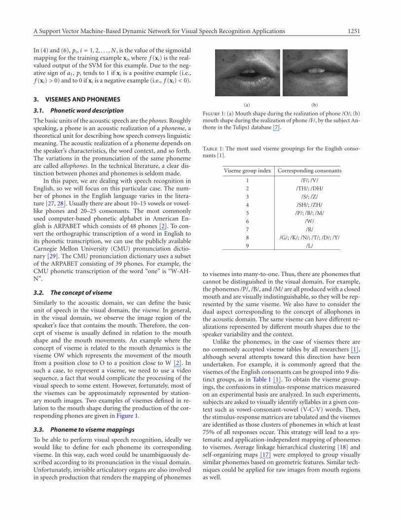
Similarly to the acoustic domain, we can define the basicunit of speech in the visual domain, the viseme. In general,in the visual domain, we observe the image region of thespeaker’s face that contains the mouth. Therefore, the con-cept of viseme is usually defined in relation to the mouthshape and the mouth movements. An example where theconcept of viseme is related to the mouth dynamics is theviseme OW which represents the movement of the mouthfrom a position close to O to a position close to W [2]. Insuch a case, to represent a viseme, we need to use a videosequence, a fact that would complicate the processing of thevisual speech to some extent. However, fortunately, most ofthe visemes can be approximately represented by station-ary mouth images. Two examples of visemes defined in re-lation to the mouth shape during the production of the cor-responding phones are given in Figure 1.

3.3. Phoneme to viseme mappings

To be able to perform visual speech recognition, ideally wewould like to define for each phoneme its correspondingviseme. In this way, each word could be unambiguously de-scribed according to its pronunciation in the visual domain.Unfortunately, invisible articulatory organs are also involvedin speech production that renders the mapping of phonemes

(a) (b)

Figure 1: (a) Mouth shape during the realization of phone /O/; (b)mouth shape during the realization of phone /F/, by the subject An-thony in the Tulips1 database [7].

Table 1: The most used viseme groupings for the English conso-nants [1].

Viseme group index Corresponding consonants

1 /F/; /V/

2 /TH/; /DH/

3 /S/; /Z/

4 /SH/; /ZH/

5 /P/; /B/; /M/

6 /W/

7 /R/

8 /G/; /K/; /N/; /T/; /D/; /Y/

9 /L/

to visemes into many-to-one. Thus, there are phonemes thatcannot be distinguished in the visual domain. For example,the phonemes /P/, /B/, and /M/ are all produced with a closedmouth and are visually indistinguishable, so they will be rep-resented by the same viseme. We also have to consider thedual aspect corresponding to the concept of allophones inthe acoustic domain. The same viseme can have different re-alizations represented by different mouth shapes due to thespeaker variability and the context.

Unlike the phonemes, in the case of visemes there areno commonly accepted viseme tables by all researchers [1],although several attempts toward this direction have beenundertaken. For example, it is commonly agreed that thevisemes of the English consonants can be grouped into 9 dis-tinct groups, as in Table 1 [1]. To obtain the viseme group-ings, the confusions in stimulus-response matrices measuredon an experimental basis are analyzed. In such experiments,subjects are asked to visually identify syllables in a given con-text such as vowel-consonant-vowel (V-C-V) words. Then,the stimulus-response matrices are tabulated and the visemesare identified as those clusters of phonemes in which at least75% of all responses occur. This strategy will lead to a sys-tematic and application-independent mapping of phonemesto visemes. Average linkage hierarchical clustering [18] andself-organizing maps [17] were employed to group visuallysimilar phonemes based on geometric features. Similar tech-niques could be applied for raw images from mouth regionsas well.

1252 EURASIP Journal on Applied Signal Processing

However, in this paper, we do not resort to such strategiesbecause our main goal is the evaluation of the proposed vi-sual speech recognition method. Thus, we define only thosevisemes that are strictly needed to represent the visual real-ization of the small vocabulary used in our application andmanually classify the training images to a number of prede-fined visemes, as explained in Section 5.

4. THE PROPOSED APPROACH TO VISUAL SPEECHRECOGNITION

Depending on the approach used to model the spoken wordsin the visual domain, we can classify the existing visualspeech recognition systems to systems using word-orientedmodels and those using viseme-oriented models [4]. In thispaper, we develop viseme-oriented models. Visemic-basedlipreading was investigated also in [17, 18]. Each visual wordmodel can be represented afterwards as a temporal sequenceof visemes. Thus, the structure of the visual word modelingand recognition system can be regarded as a two-level struc-ture.

(1) At the first level, we build the viseme classes, one classof mouth images for each viseme defined. This implies theformulation of the mouth shape recognition problem as apattern recognition problem. The patterns to be recognizedare the mouth shapes, symbolically represented as visemes.In our approach, the classification of mouth shapes to visemeclasses is formulated as a two-class (binary) pattern recogni-tion problem and there is one SVM dedicated for each visemeclass.

(2) At the second level, we build the abstract visual wordmodels described as temporal sequences of visemes. The vi-sual word models are implemented by means of the Viterbilattices where each node generates the emission probabilityof a certain viseme at one particular time instant.

Notice that the aforementioned two-level approach isvery similar to some techniques employed for acoustic speechrecognition [16], justifying thus our expectation that theproposed method will ensure an easy integration of the visualspeech recognition subsystem with a similar acoustic speechrecognition subsystem.

In this section, we focus on the first level of the proposedalgorithm for visual speech modeling and recognition. Thesecond level involves the development of the visual symbolicsequential word models using the Viterbi lattices. The latterlevel is discussed only in principle.

4.1. Formulation of visual speech recognitionas a pattern recognition problem

The problem of discriminating between different mouthshapes during speech production can be viewed as a patternrecognition problem. In this case, the set of patterns is a setof feature vectors {xi}, i = 1, 2, . . . , P, each of them describ-ing some mouth shape. The feature vector xi is a represen-tation of the mouth image. The feature vector xi can repre-sent the mouth image at low level (i.e., the gray levels froma rectangular image region containing the mouth). It cancomprise geometric parameters (i.e., mouth width, height,

perimeter, etc.) or the coefficients of a linear transformationof the mouth image. All the feature vectors from the set havethe same number of components M.

Denote the pattern classes by � j , j = 1, 2, . . . , Q, whereQ is the total number of classes. Each class � j is a group ofpatterns that represent mouth shapes corresponding to oneviseme.

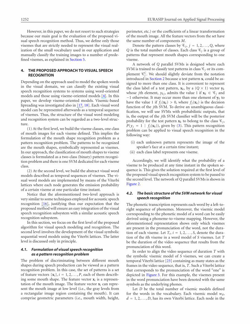
A network of Q parallel SVMs is designed where eachSVM is trained to classify test patterns in class � j or its com-plement �C

j . We should slightly deviate from the notationintroduced in Section 2 because a test pattern xi could be as-signed to more than one class. It is convenient to representthe class label of a test pattern, xk, by a (Q × 1) vector ykwhose jth element, yk j , admits the value 1 if xk ∈ � j and−1 otherwise. It may occur more than one element of yk tohave the value 1 if f j(xk) > 0, where f j(xk) is the decisionfunction of the jth SVM. To derive an unambiguous classi-fication, we will use SVMs with probabilistic outputs, thatis, the output of the jth SVM classifier will be the posteriorprobability for the test pattern xk to belong to the class � j ,P(yj = 1 | f j(xk)), given by (3). This pattern recognitionproblem can be applied to visual speech recognition in thefollowing way:

(i) each unknown pattern represents the image of thespeaker’s face at a certain time instant;

(ii) each class label represents one viseme.

Accordingly, we will identify what the probability of aviseme to be produced at any time instant in the spoken se-quence is. This gives the solution required at the first level ofthe proposed visual speech recognition system to be passed tothe second level. The network of Q parallel SVMs is shown inFigure 2.

4.2. The basic structure of the SVM network for visualspeech recognition

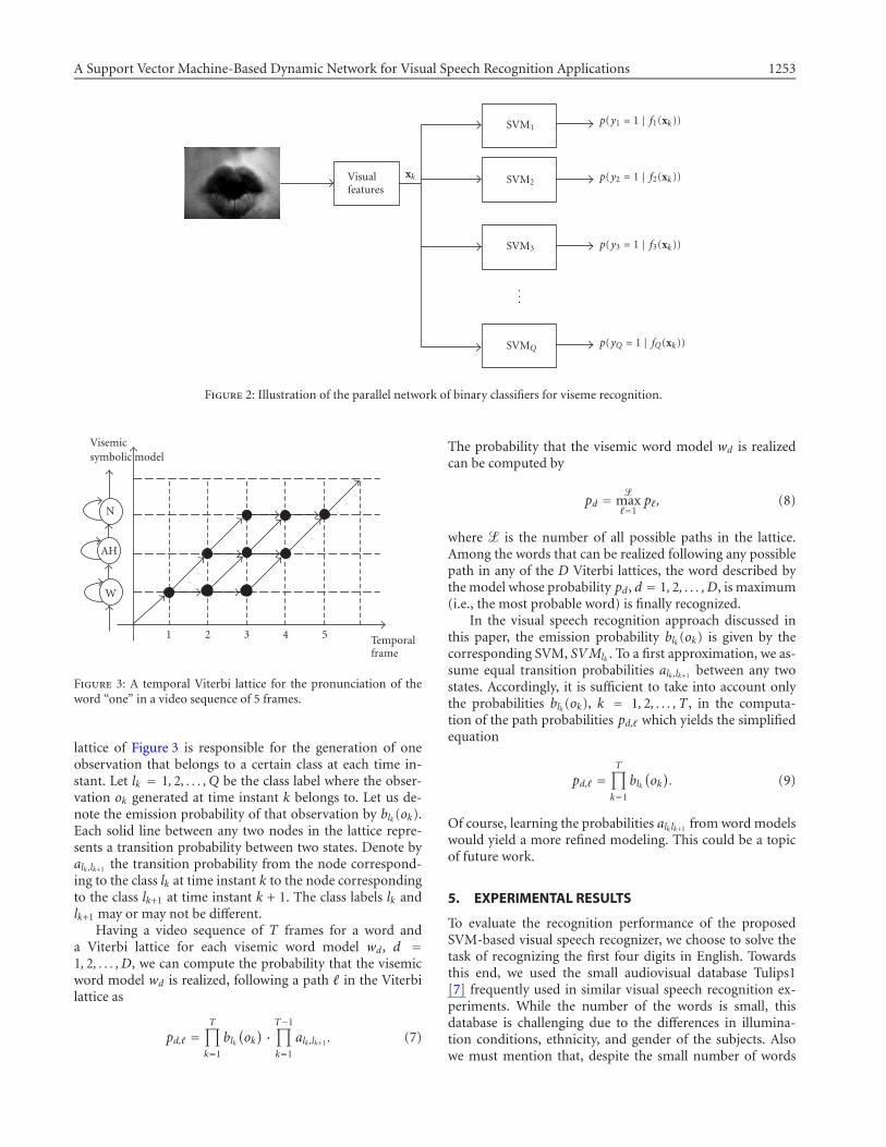
The phonetic transcription represents each word by a left-to-right sequence of phonemes. Moreover, the visemic modelcorresponding to the phonetic model of a word can be easilyderived using a phoneme-to-viseme mapping. However, theaforementioned representation shows only which visemesare present in the pronunciation of the word, not the dura-tion of each viseme. Let Ti, i = 1, 2, . . . , S, denote the dura-tion of the ith viseme in a word model of S visemes. Let Tbe the duration of the video sequence that results from thepronunciation of this word.

In order to align the video sequence of duration T withthe symbolic visemic model of S visemes, we can create atemporal Viterbi lattice [23] containing as many states as theframes in the video sequence, that is, T . Such a Viterbi latticethat corresponds to the pronunciation of the word “one” isdepicted in Figure 3. For this example, the visemes presentin the word pronunciation have been denoted with the samesymbols as the underlying phones.

Let D be the total number of visemic models definedfor the words in the vocabulary. Each visemic model wd,d = 1, 2, . . . , D, has its own Viterbi lattice. Each node in the

A Support Vector Machine-Based Dynamic Network for Visual Speech Recognition Applications 1253

p(yQ = 1 | fQ(xk))

p(y3 = 1 | f3(xk))

p(y2 = 1 | f2(xk))

p(y1 = 1 | f1(xk))

...

SVMQ

SVM3

SVM2

SVM1

xkVisualfeatures

Figure 2: Illustration of the parallel network of binary classifiers for viseme recognition.

Temporalframe

54321

W

AH

N

Visemicsymbolic model

Figure 3: A temporal Viterbi lattice for the pronunciation of theword “one” in a video sequence of 5 frames.

lattice of Figure 3 is responsible for the generation of oneobservation that belongs to a certain class at each time in-stant. Let lk = 1, 2, . . . , Q be the class label where the obser-vation ok generated at time instant k belongs to. Let us de-note the emission probability of that observation by blk (ok).Each solid line between any two nodes in the lattice repre-sents a transition probability between two states. Denote byalk,lk+1 the transition probability from the node correspond-ing to the class lk at time instant k to the node correspondingto the class lk+1 at time instant k + 1. The class labels lk andlk+1 may or may not be different.

Having a video sequence of T frames for a word anda Viterbi lattice for each visemic word model wd, d =1, 2, . . . , D, we can compute the probability that the visemicword model wd is realized, following a path � in the Viterbilattice as

pd,� =T∏

k=1

blk(ok) · T−1∏

k=1

alk,lk+1 . (7)

The probability that the visemic word model wd is realizedcan be computed by

pd = �max�=1

p�, (8)

where � is the number of all possible paths in the lattice.Among the words that can be realized following any possiblepath in any of the D Viterbi lattices, the word described bythe model whose probability pd, d = 1, 2, . . . , D, is maximum(i.e., the most probable word) is finally recognized.

In the visual speech recognition approach discussed inthis paper, the emission probability blk (ok) is given by thecorresponding SVM, SVMlk . To a first approximation, we as-sume equal transition probabilities alk,lk+1 between any twostates. Accordingly, it is sufficient to take into account onlythe probabilities blk (ok), k = 1, 2, . . . , T , in the computa-tion of the path probabilities pd,� which yields the simplifiedequation

pd,� =T∏

k=1

blk(ok). (9)

Of course, learning the probabilities alklk+1 from word modelswould yield a more refined modeling. This could be a topicof future work.

5. EXPERIMENTAL RESULTS

To evaluate the recognition performance of the proposedSVM-based visual speech recognizer, we choose to solve thetask of recognizing the first four digits in English. Towardsthis end, we used the small audiovisual database Tulips1[7] frequently used in similar visual speech recognition ex-periments. While the number of the words is small, thisdatabase is challenging due to the differences in illumina-tion conditions, ethnicity, and gender of the subjects. Alsowe must mention that, despite the small number of words

1254 EURASIP Journal on Applied Signal Processing

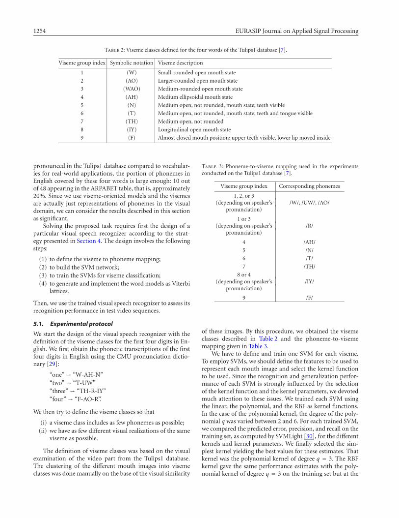
Table 2: Viseme classes defined for the four words of the Tulips1 database [7].

Viseme group index Symbolic notation Viseme description

1 (W) Small-rounded open mouth state

2 (AO) Larger-rounded open mouth state

3 (WAO) Medium-rounded open mouth state

4 (AH) Medium ellipsoidal mouth state

5 (N) Medium open, not rounded, mouth state; teeth visible

6 (T) Medium open, not rounded, mouth state; teeth and tongue visible

7 (TH) Medium open, not rounded

8 (IY) Longitudinal open mouth state

9 (F) Almost closed mouth position; upper teeth visible, lower lip moved inside

pronounced in the Tulips1 database compared to vocabular-ies for real-world applications, the portion of phonemes inEnglish covered by these four words is large enough: 10 outof 48 appearing in the ARPABET table, that is, approximately20%. Since we use viseme-oriented models and the visemesare actually just representations of phonemes in the visualdomain, we can consider the results described in this sectionas significant.

Solving the proposed task requires first the design of aparticular visual speech recognizer according to the strat-egy presented in Section 4. The design involves the followingsteps:

(1) to define the viseme to phoneme mapping;(2) to build the SVM network;(3) to train the SVMs for viseme classification;(4) to generate and implement the word models as Viterbi

lattices.

Then, we use the trained visual speech recognizer to assess itsrecognition performance in test video sequences.

5.1. Experimental protocol

We start the design of the visual speech recognizer with thedefinition of the viseme classes for the first four digits in En-glish. We first obtain the phonetic transcriptions of the firstfour digits in English using the CMU pronunciation dictio-nary [29]:

“one”→ “W-AH-N”“two”→ “T-UW”“three”→ “TH-R-IY”“four”→ “F-AO-R”.

We then try to define the viseme classes so that

(i) a viseme class includes as few phonemes as possible;(ii) we have as few different visual realizations of the same

viseme as possible.

The definition of viseme classes was based on the visualexamination of the video part from the Tulips1 database.The clustering of the different mouth images into visemeclasses was done manually on the base of the visual similarity

Table 3: Phoneme-to-viseme mapping used in the experimentsconducted on the Tulips1 database [7].

Viseme group index Corresponding phonemes

1, 2, or 3(depending on speaker’s /W/, /UW/, /AO/

pronunciation)

1 or 3(depending on speaker’s /R/

pronunciation)

4 /AH/

5 /N/

6 /T/

7 /TH/

8 or 4(depending on speaker’s /IY/

pronunciation)

9 /F/

of these images. By this procedure, we obtained the visemeclasses described in Table 2 and the phoneme-to-visememapping given in Table 3.

We have to define and train one SVM for each viseme.To employ SVMs, we should define the features to be used torepresent each mouth image and select the kernel functionto be used. Since the recognition and generalization perfor-mance of each SVM is strongly influenced by the selectionof the kernel function and the kernel parameters, we devotedmuch attention to these issues. We trained each SVM usingthe linear, the polynomial, and the RBF as kernel functions.In the case of the polynomial kernel, the degree of the poly-nomial q was varied between 2 and 6. For each trained SVM,we compared the predicted error, precision, and recall on thetraining set, as computed by SVMLight [30], for the differentkernels and kernel parameters. We finally selected the sim-plest kernel yielding the best values for these estimates. Thatkernel was the polynomial kernel of degree q = 3. The RBFkernel gave the same performance estimates with the poly-nomial kernel of degree q = 3 on the training set but at the

A Support Vector Machine-Based Dynamic Network for Visual Speech Recognition Applications 1255

cost of a larger number of support vectors. A simple choiceof a feature vector such as the collection of the gray levelsfrom a rectangular region of fixed size containing the mouth,scanned row by row, is proved suitable whenever SVMs havebeen used for visual classification tasks [15]. More specifi-cally, we used two types of features to conduct the visualspeech recognition experiments.

(i) The first type comprised the gray levels of a rectangu-lar region of interest around the mouth, downsampled to thesize 16 × 16. Each mouth image is represented by a featurevector of length 256.

(ii) The second type represented each mouth imageframe at the time Tf by a vector of double size (i.e., 512) thatcomprised the gray levels of the rectangular region of interestaround the mouth downsampled to the size 16 × 16, as pre-viously. The temporal derivatives of the gray levels normal-ized to the range [0, Lmax − 1], where Lmax is the maximumgray level value in mouth image. The temporal derivativesare simply the pixel by pixel gray level differences betweenthe frames Tf and Tf − 1. These differences are the so-calleddelta features.

Some preprocessing of the mouth images was needed be-fore training and testing the visual speech recognition sys-tem. It concerns the normalization of the mouth in scale, ro-tation, and position inside the image. Such a preprocessingis needed due to the fact that the mouth has different scale,position in the image, and orientation toward the horizon-tal axis from utterance to utterance depending on the subjectand on its position in front of the camera. To compensate forthese variations, we applied the normalization procedure ofmouth images with respect to scale, translation, and rotationdescribed in [6].

The visual speech recognizer was tested for speaker-independent recognition using the leave-one-out testingstrategy for the 12 subjects in the Tulips1 database. This im-plies training the visual speech recognizer 12 times, each timeusing only 11 subjects for training and leaving the 12th outfor testing. In each case, we trained first the SVMs, and thenthe sigmoidal mappings for converting the SVMs output toprobabilities. The training set, for each SVM in each systemconfiguration is defined manually. Only the video sequences,from the so-called Set 1 from the Tulips1 database, were usedfor training. The labeling of all the frames from Set 1 (a totalof 48 video sequences) was done manually by visual exami-nation of each frame. We examined the video only to label allthe frames according to Table 3 except the transition framesbetween two visemes denoting differently the same visemeclass for each subject. Finally, we compared the similarity ofthe frames corresponding to the same viseme and differentsubjects and decided if the classes could be merged. The dis-advantage of this approach is the large time needed for la-beling, which would not be needed if HMMs were used forsegmentation. A compromise solution for labeling could bethe use of an automatic solution for phoneme-level segmen-tation of the audio sequence and the use of this segmentationon the aligned video sequence also.

Once the labeling was done, only the unambiguous posi-tive and negative viseme examples were included in the train-

ing sets. The feature vectors used in the training sets of allSVMs were the same. Only their labeling as positive or neg-ative examples differs from one SVM to another. This leadsto an unbalanced training set in the sense that the negativeexamples are frequently more than the positive ones.

The configuration of the Viterbi lattice depends on thelength of the test sequence through the number of framesTtest of the sequence (as illustrated in Figure 3). It was gen-erated automatically at runtime for each test sequence. Thenumber of Viterbi lattices can be determined in advance, be-cause it is equal to the total number of visemic word models.Thus, taking into account the phonetic descriptions for thefour words of the vocabulary and the phoneme-to-visememappings in Table 3, we have 3 visemic word models for theword “one,” 3 models for “two,” 4 models for “three,” and 6models for “four.” The multiple visemic models per word aredue to the variability in speakers’ pronunciation.

In each of the 12 leave-one-out tests, we have as test se-quences, the video sequences corresponding to the pronun-ciation of the four words and there are two pronunciationsavailable for each word and the speaker. This leads to a subto-tal of 8 test sequences per system configuration, and a total of12× 8 = 96 test sequences for the visual speech recognizer.

The complete visual speech recognizer was implementedin C++. We used the publicly available SVMLight toolkitmodules for the training of the SVMs [30]. We implementedin C++, the module for learning the sigmoidal mappings ofthe SVMs output to probabilities and the module for gener-ating the Viterbi lattice models based on SVMs with prob-abilistic outputs. All these modules were integrated into thevisual speech recognition system whose architecture is struc-tured into two modules: the training module and the testmodule.

Two visual speech recognizers were implemented,trained, and tested with the aforementioned strategy. Theydiffer in the type of features used. The first system (with-out delta features) did not include temporal derivatives inthe feature vector, while the second (with delta features) in-cluded also temporal derivatives between two frames in thefeature vector.

5.2. Performance evaluation

In this section, we present the experimental results obtainedwith the proposed system with or without using delta fea-tures. Moreover, we compare these results to others reportedin the literature for the same experiment on the Tulips1database. The word recognition rates (WRR) have been aver-aged over the 96 tests obtained by applying the leave-one-outprinciple. Five figures of merit are provided.

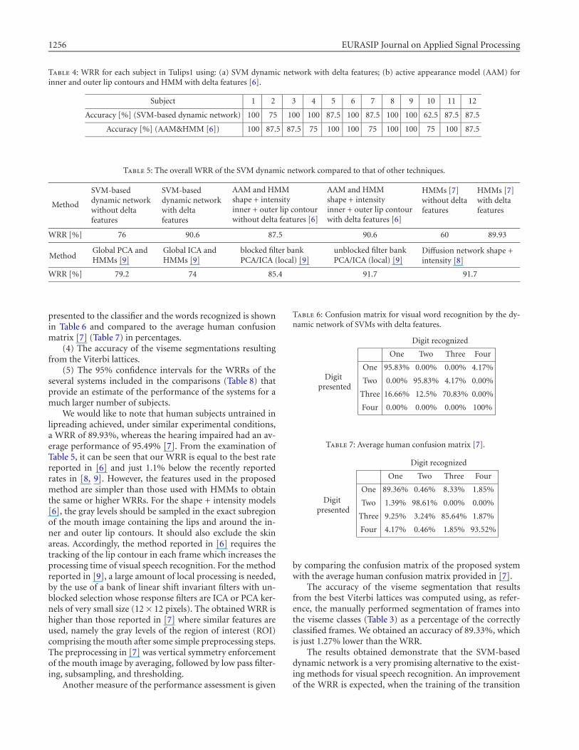
(1) The WRR per subject, obtained by the proposedmethod when delta features are used, is measured and com-pared to that by Luettin and Thacker [6] (Table 4).

(2) The overall WRR for all subjects and pronunciations,with and without delta features, is reported compared to thatobtained by Luettin and Thacker [6], Movellan [7], Gray etal. [9], and Movellan et al. [8] (Table 5).

(3) The confusion matrix between the words actually

1256 EURASIP Journal on Applied Signal Processing

Table 4: WRR for each subject in Tulips1 using: (a) SVM dynamic network with delta features; (b) active appearance model (AAM) forinner and outer lip contours and HMM with delta features [6].

Subject 1 2 3 4 5 6 7 8 9 10 11 12

Accuracy [%] (SVM-based dynamic network) 100 75 100 100 87.5 100 87.5 100 100 62.5 87.5 87.5

Accuracy [%] (AAM&HMM [6]) 100 87.5 87.5 75 100 100 75 100 100 75 100 87.5

Table 5: The overall WRR of the SVM dynamic network compared to that of other techniques.

Method

SVM-baseddynamic networkwithout deltafeatures

SVM-baseddynamic networkwith deltafeatures

AAM and HMMshape + intensityinner + outer lip contourwithout delta features [6]

AAM and HMMshape + intensityinner + outer lip contourwith delta features [6]

HMMs [7]without deltafeatures

HMMs [7]with deltafeatures

WRR [%] 76 90.6 87.5 90.6 60 89.93

MethodGlobal PCA andHMMs [9]

Global ICA andHMMs [9]

blocked filter bankPCA/ICA (local) [9]

unblocked filter bankPCA/ICA (local) [9]

Diffusion network shape +intensity [8]

WRR [%] 79.2 74 85.4 91.7 91.7

presented to the classifier and the words recognized is shownin Table 6 and compared to the average human confusionmatrix [7] (Table 7) in percentages.

(4) The accuracy of the viseme segmentations resultingfrom the Viterbi lattices.

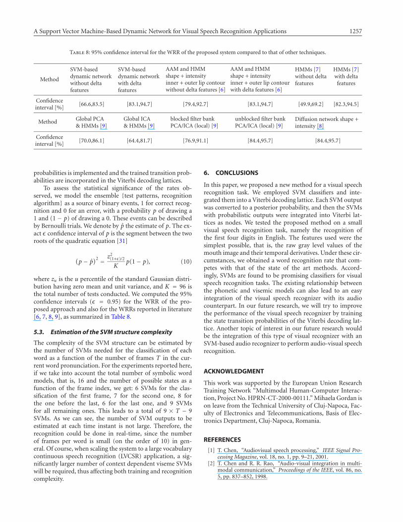
(5) The 95% confidence intervals for the WRRs of theseveral systems included in the comparisons (Table 8) thatprovide an estimate of the performance of the systems for amuch larger number of subjects.

We would like to note that human subjects untrained inlipreading achieved, under similar experimental conditions,a WRR of 89.93%, whereas the hearing impaired had an av-erage performance of 95.49% [7]. From the examination ofTable 5, it can be seen that our WRR is equal to the best ratereported in [6] and just 1.1% below the recently reportedrates in [8, 9]. However, the features used in the proposedmethod are simpler than those used with HMMs to obtainthe same or higher WRRs. For the shape + intensity models[6], the gray levels should be sampled in the exact subregionof the mouth image containing the lips and around the in-ner and outer lip contours. It should also exclude the skinareas. Accordingly, the method reported in [6] requires thetracking of the lip contour in each frame which increases theprocessing time of visual speech recognition. For the methodreported in [9], a large amount of local processing is needed,by the use of a bank of linear shift invariant filters with un-blocked selection whose response filters are ICA or PCA ker-nels of very small size (12× 12 pixels). The obtained WRR ishigher than those reported in [7] where similar features areused, namely the gray levels of the region of interest (ROI)comprising the mouth after some simple preprocessing steps.The preprocessing in [7] was vertical symmetry enforcementof the mouth image by averaging, followed by low pass filter-ing, subsampling, and thresholding.

Another measure of the performance assessment is given

Table 6: Confusion matrix for visual word recognition by the dy-namic network of SVMs with delta features.

Digit recognized

Digitpresented

One Two Three Four

One 95.83% 0.00% 0.00% 4.17%

Two 0.00% 95.83% 4.17% 0.00%

Three 16.66% 12.5% 70.83% 0.00%

Four 0.00% 0.00% 0.00% 100%

Table 7: Average human confusion matrix [7].

Digit recognized

One Two Three Four

One 89.36% 0.46% 8.33% 1.85%Digit

presentedTwo 1.39% 98.61% 0.00% 0.00%

Three 9.25% 3.24% 85.64% 1.87%

Four 4.17% 0.46% 1.85% 93.52%

by comparing the confusion matrix of the proposed systemwith the average human confusion matrix provided in [7].

The accuracy of the viseme segmentation that resultsfrom the best Viterbi lattices was computed using, as refer-ence, the manually performed segmentation of frames intothe viseme classes (Table 3) as a percentage of the correctlyclassified frames. We obtained an accuracy of 89.33%, whichis just 1.27% lower than the WRR.

The results obtained demonstrate that the SVM-baseddynamic network is a very promising alternative to the exist-ing methods for visual speech recognition. An improvementof the WRR is expected, when the training of the transition

A Support Vector Machine-Based Dynamic Network for Visual Speech Recognition Applications 1257

Table 8: 95% confidence interval for the WRR of the proposed system compared to that of other techniques.

Method

SVM-baseddynamic networkwithout deltafeatures

SVM-baseddynamic networkwith deltafeatures

AAM and HMMshape + intensityinner + outer lip contourwithout delta features [6]

AAM and HMMshape + intensityinner + outer lip contourwith delta features [6]

HMMs [7]without deltafeatures

HMMs [7]with deltafeatures

Confidenceinterval [%]

[66.6,83.5] [83.1,94.7] [79.4,92.7] [83.1,94.7] [49.9,69.2] [82.3,94.5]

Method Global PCA& HMMs [9]

Global ICA& HMMs [9]

blocked filter bankPCA/ICA (local) [9]

unblocked filter bankPCA/ICA (local) [9]

Diffusion network shape +intensity [8]

Confidenceinterval [%]

[70.0,86.1] [64.4,81.7] [76.9,91.1] [84.4,95.7] [84.4,95.7]

probabilities is implemented and the trained transition prob-abilities are incorporated in the Viterbi decoding lattices.

To assess the statistical significance of the rates ob-served, we model the ensemble {test patterns, recognitionalgorithm} as a source of binary events, 1 for correct recog-nition and 0 for an error, with a probability p of drawing a1 and (1 − p) of drawing a 0. These events can be describedby Bernoulli trials. We denote by p̂ the estimate of p. The ex-act ε confidence interval of p is the segment between the tworoots of the quadratic equation [31]

(p − p̂

)2 = z2(1+ε)/2

Kp(1− p), (10)

where zu is the u percentile of the standard Gaussian distri-bution having zero mean and unit variance, and K = 96 isthe total number of tests conducted. We computed the 95%confidence intervals (ε = 0.95) for the WRR of the pro-posed approach and also for the WRRs reported in literature[6, 7, 8, 9], as summarized in Table 8.

5.3. Estimation of the SVM structure complexity

The complexity of the SVM structure can be estimated bythe number of SVMs needed for the classification of eachword as a function of the number of frames T in the cur-rent word pronunciation. For the experiments reported here,if we take into account the total number of symbolic wordmodels, that is, 16 and the number of possible states as afunction of the frame index, we get: 6 SVMs for the clas-sification of the first frame, 7 for the second one, 8 forthe one before the last, 6 for the last one, and 9 SVMsfor all remaining ones. This leads to a total of 9 × T − 9SVMs. As we can see, the number of SVM outputs to beestimated at each time instant is not large. Therefore, therecognition could be done in real-time, since the numberof frames per word is small (on the order of 10) in gen-eral. Of course, when scaling the system to a large vocabularycontinuous speech recognition (LVCSR) application, a sig-nificantly larger number of context dependent viseme SVMswill be required, thus affecting both training and recognitioncomplexity.

6. CONCLUSIONS

In this paper, we proposed a new method for a visual speechrecognition task. We employed SVM classifiers and inte-grated them into a Viterbi decoding lattice. Each SVM outputwas converted to a posterior probability, and then the SVMswith probabilistic outputs were integrated into Viterbi lat-tices as nodes. We tested the proposed method on a smallvisual speech recognition task, namely the recognition ofthe first four digits in English. The features used were thesimplest possible, that is, the raw gray level values of themouth image and their temporal derivatives. Under these cir-cumstances, we obtained a word recognition rate that com-petes with that of the state of the art methods. Accord-ingly, SVMs are found to be promising classifiers for visualspeech recognition tasks. The existing relationship betweenthe phonetic and visemic models can also lead to an easyintegration of the visual speech recognizer with its audiocounterpart. In our future research, we will try to improvethe performance of the visual speech recognizer by trainingthe state transition probabilities of the Viterbi decoding lat-tice. Another topic of interest in our future research wouldbe the integration of this type of visual recognizer with anSVM-based audio recognizer to perform audio-visual speechrecognition.

ACKNOWLEDGMENT

This work was supported by the European Union ResearchTraining Network “Multimodal Human-Computer Interac-tion, Project No. HPRN-CT-2000-00111.” Mihaela Gordan ison leave from the Technical University of Cluj-Napoca, Fac-ulty of Electronics and Telecommunications, Basis of Elec-tronics Department, Cluj-Napoca, Romania.

REFERENCES

[1] T. Chen, “Audiovisual speech processing,” IEEE Signal Pro-cessing Magazine, vol. 18, no. 1, pp. 9–21, 2001.

[2] T. Chen and R. R. Rao, “Audio-visual integration in multi-modal communication,” Proceedings of the IEEE, vol. 86, no.5, pp. 837–852, 1998.

1258 EURASIP Journal on Applied Signal Processing

[3] C. Benoı̂t, T. Lallouache, T. Mohamadi, and C. Abry, “A setof French visemes for visual speech synthesis,” in Talking Ma-chines: Theories, Models, and Designs, G. Bailly and C. Benoı̂t,Eds., pp. 485–504, Elsevier-North Holland, Amsterdam, 1992.

[4] C. Neti, G. Potamianos, J. Luettin, I. Matthews, H. Glotin, andD. Vergyri, “Large-vocabulary audio-visual speech recogni-tion: a summary of the Johns Hopkins summer 2000 work-shop,” in Proc. IEEE Workshop Multimedia Signal Processing,pp. 619–624, Cannes, France, 2001.

[5] C. Bregler and S. Omohundro, “Nonlinear manifold learn-ing for visual speech recognition,” in Proc. IEEE InternationalConf. on Computer Vision, pp. 494–499, Cambridge, Mass,USA, 1995.

[6] J. Luettin and N. A. Thacker, “Speechreading using proba-bilistic models,” Computer Vision and Image Understanding,vol. 65, no. 2, pp. 163–178, 1997.

[7] J. R. Movellan, “Visual speech recognition with stochastic net-works,” in Advances in Neural Information Processing Systems,G. Tesauro, D. Toruetzky, and T. Leen, Eds., vol. 7, pp. 851–858, MIT Press, Cambridge, Mass, USA, 1995.

[8] J. R. Movellan, P. Mineiro, and R. J. Williams, “Partially ob-servable SDE models for image sequence recognition tasks,”in Advances in Neural Information Processing Systems, T. Leen,T. G. Dietterich, and V. Tresp, Eds., vol. 13, pp. 880–886, MITPress, Cambridge, Mass, USA, 2001.

[9] M. S. Gray, T. J. Sejnowski, and J. R. Movellan, “A comparisonof image processing techniques for visual speech recognitionapplications,” in Advances in Neural Information ProcessingSystems, T. Leen, T. G. Dietterich, and V. Tresp, Eds., vol. 13,pp. 939–945, MIT Press, Cambridge, Mass, USA, 2001.

[10] Y. Li, S. Gong, and H. Liddell, “Support vector regressionand classification based multi-view face detection and recog-nition,” in Proc. 4th IEEE Int. Conf. Automatic Face and Ges-ture Recognition, pp. 300–305, Grenoble, France, 2000.

[11] T.-J. Terrillon, M. N. Shirazi, M. Sadek, H. Fukamachi, andS. Akamatsu, “Invariant face detection with support vectormachines,” in Proc. 15th Int. Conf. Pattern Recognition, vol. 4,pp. 210–217, Barcelona, Spain, 2000.

[12] A. Tefas, C. Kotropoulos, and I. Pitas, “Using support vectormachines to enhance the performance of elastic graph match-ing for frontal face authentication,” IEEE Trans. on PatternAnalysis and Machine Intelligence, vol. 23, no. 7, pp. 735–746,2001.

[13] C. Kotropoulos, N. Bassiou, T. Kosmidis, and I. Pitas, “Frontalface detection using support vector machines and back-propagation neural networks,” in Proc. 2001 ScandinavianConf. Image Analysis (SCIA ’01), pp. 199–206, Bergen, Nor-way, 2001.

[14] A. Fazekas, C. Kotropoulos, I. Buciu, and I. Pitas, “Supportvector machines on the space of Walsh functions and theirproperties,” in Proc. 2nd IEEE Int. Symp. Image and SignalProcessing and Applications, pp. 43–48, Pula, Croatia, 2001.

[15] I. Buciu, C. Kotropoulos, and I. Pitas, “Combining supportvector machines for accurate face detection,” in Proc. 2001IEEE Int. Conf. Image Processing, vol. 1, pp. 1054–1057, Thes-saloniki, Greece, October 2001.

[16] A. Ganapathiraju, J. Hamaker, and J. Picone, “HybridSVM/HMM architectures for speech recognition,” in Proc.Speech Transcription Workshop, College Park, Md, USA, 2000.

[17] A. Rogozan, “Discriminative learning of visual data for audio-visual speech recognition,” International Journal on ArtificialIntelligence Tools, vol. 8, no. 1, pp. 43–52, 1999.

[18] A. J. Goldschen, Continuous automatic speech recognitionby lipreading, Ph.D. thesis, George Washington University,Washington, DC, USA, 1993.

[19] A. J. Goldschen, O. N. Garcia, and E. D. Petajan, “Ratio-nale for phoneme-viseme mapping and feature selection invisual speech recognition,” in Speechreading by Humans andMachines: Models, Systems, and Applications, D. G. Stork andM. E. Hennecke, Eds., pp. 505–515, Springer-Verlag, Berlin,Germany, 1996.

[20] J. R. Movellan and J. L. McClelland, “The Morton-Massarolaw of information integration: Implications for models ofperception,” Psychological Review, vol. 108, no. 1, pp. 113–148, 2001.

[21] V. N. Vapnik, Statistical Learning Theory, John Wiley, NewYork, NY, USA, 1998.

[22] N. Cristianini and J. Shawe-Taylor, An Introduction to SupportVector Machines, Cambridge University Press, Cambridge,UK, 2000.

[23] S. Young, D. Kershaw, J. Odell, D. Ollason, V. Valtchev, andP. Woodland, The HTK Book, Entropic, Cambridge, UK,1999, HTK version 2.2.

[24] J. T.-Y. Kwok, “Moderating the outputs of support vector ma-chine classifiers,” IEEE Trans. Neural Networks, vol. 10, no. 5,pp. 1018–1031, 1999.

[25] J. Platt, “Probabilistic outputs for support vector machinesand comparisons to regularized likelihood methods,” inAdvances in Large Margin Classifiers, A. Smola, P. Bartlett,B. Scholkopf, and D. Schuurmans, Eds., MIT Press, Cam-bridge, Mass, USA, 2000.

[26] T. Hastie and R. Tibshirani, “Classification by pairwise cou-pling,” The Annals of Statistics, vol. 26, no. 1, pp. 451–471,1998.

[27] J. R. Deller, J. G. Proakis, and J. H. L. Hansen, Discrete-Time Processing of Speech Signals, Prentice-Hall, Upper SaddleRiver, NJ, USA, 1993.

[28] L. Rabiner and B.-H. Juang, Fundamentals of Speech Recogni-tion, Prentice-Hall, Englewood Cliffs, NJ, USA, 1993.

[29] The Carnegie Mellon University Pronouncing Dictionary V.0.6, http://www.speech.cs.cmu.edu/cgi-bin/cmudict.

[30] T. Joachims, “Making large-scale SVM learning practi-cal,” in Advances in Kernel Methods—Support Vector Learn-ing, B. Scoelkopf, C. Burges, and A. Smola, Eds., MIT Press,Cambridge, Mass, USA, 1999.

[31] A. Papoulis, Probability, Random Variables, and Stochastic Pro-cesses, McGraw-Hill, New York, NY, USA, 3rd edition, 1991.

Mihaela Gordan received the Diploma inelectronics engineering in 1995 and theM.S. degree in electronics in 1996, bothfrom the Technical University of Cluj-Napoca, Cluj-Napoca, Romania. Currently,she is working on her Ph.D. degree in elec-tronics and communications at the Basisof Electronics Department of the TechnicalUniversity of Cluj-Napoca where she servesas a Teaching Assistant since 1997. Ms. Gor-dan authored a number of 30 conference and journal papers and1 book in her area of expertise. Her current research interests in-clude applied fuzzy logic in image processing, pattern recognition,human-computer interaction, visual speech recognition, and sup-port vector machines. Ms. Gordan is a student member of IEEE andmember of the Signal Processing Society of IEEE since 1999.

A Support Vector Machine-Based Dynamic Network for Visual Speech Recognition Applications 1259

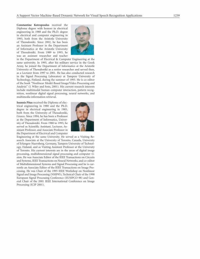
Constantine Kotropoulos received theDiploma degree with honors in electricalengineering in 1988 and the Ph.D. degreein electrical and computer engineering in1993, both from the Aristotle Universityof Thessaloniki. Since 2002, he has beenan Assistant Professor in the Departmentof Informatics at the Aristotle Universityof Thessaloniki. From 1989 to 1993, hewas an assistant researcher and teacherin the Department of Electrical & Computer Engineering at thesame university. In 1995, after his military service in the GreekArmy, he joined the Department of Informatics at the AristotleUniversity of Thessaloniki as a senior researcher and served then,as a Lecturer from 1997 to 2001. He has also conducted researchin the Signal Processing Laboratory at Tampere University ofTechnology, Finland, during the summer of 1993. He is co-editorof the book “Nonlinear Model-Based Image/Video Processing andAnalysis” (J. Wiley and Sons, 2001). His current research interestsinclude multimodal human computer interaction, pattern recog-nition, nonlinear digital signal processing, neural networks, andmultimedia information retrieval.

Ioannis Pitas received the Diploma of elec-trical engineering in 1980 and the Ph.D.degree in electrical engineering in 1985,both from the University of Thessaloniki,Greece. Since 1994, he has been a Professorat the Department of Informatics, Univer-sity of Thessaloniki. From 1980 to 1993, heserved as Scientific Assistant, Lecturer, As-sistant Professor, and Associate Professor inthe Department of Electrical and ComputerEngineering at the same University. He served as a Visiting Re-search Associate at the University of Toronto, Canada, Universityof Erlangen-Nuernberg, Germany, Tampere University of Technol-ogy, Finland, and as Visiting Assistant Professor at the Universityof Toronto. His current interests are in the areas of digital imageprocessing, multidimensional signal processing and computer vi-sion. He was Associate Editor of the IEEE Transactions on Circuitsand Systems, IEEE Transactions on Neural Networks, and co-editorof Multidimensional Systems and Signal Processing and he is cur-rently an Associate Editor of the IEEE Transactions on Image Pro-cessing. He was Chair of the 1995 IEEE Workshop on NonlinearSignal and Image Processing (NSIP95), Technical Chair of the 1998European Signal Processing Conference (EUSIPCO 98) and Gen-eral Chair of the 2001 IEEE International Conference on ImageProcessing (ICIP 2001).

Photograph © Turisme de Barcelona / J. Trullàs

Preliminary call for papers

The 2011 European Signal Processing Conference (EUSIPCO 2011) is thenineteenth in a series of conferences promoted by the European Association forSignal Processing (EURASIP, www.eurasip.org). This year edition will take placein Barcelona, capital city of Catalonia (Spain), and will be jointly organized by theCentre Tecnològic de Telecomunicacions de Catalunya (CTTC) and theUniversitat Politècnica de Catalunya (UPC).EUSIPCO 2011 will focus on key aspects of signal processing theory and

li ti li t d b l A t f b i i ill b b d lit

Organizing Committee

Honorary ChairMiguel A. Lagunas (CTTC)

General ChairAna I. Pérez Neira (UPC)

General Vice ChairCarles Antón Haro (CTTC)

Technical Program ChairXavier Mestre (CTTC)

Technical Program Co Chairsapplications as listed below. Acceptance of submissions will be based on quality,relevance and originality. Accepted papers will be published in the EUSIPCOproceedings and presented during the conference. Paper submissions, proposalsfor tutorials and proposals for special sessions are invited in, but not limited to,the following areas of interest.

Areas of Interest

• Audio and electro acoustics.• Design, implementation, and applications of signal processing systems.

l d l d d

Technical Program Co ChairsJavier Hernando (UPC)Montserrat Pardàs (UPC)

Plenary TalksFerran Marqués (UPC)Yonina Eldar (Technion)

Special SessionsIgnacio Santamaría (Unversidadde Cantabria)Mats Bengtsson (KTH)

FinancesMontserrat Nájar (UPC)• Multimedia signal processing and coding.

• Image and multidimensional signal processing.• Signal detection and estimation.• Sensor array and multi channel signal processing.• Sensor fusion in networked systems.• Signal processing for communications.• Medical imaging and image analysis.• Non stationary, non linear and non Gaussian signal processing.

Submissions

Montserrat Nájar (UPC)

TutorialsDaniel P. Palomar(Hong Kong UST)Beatrice Pesquet Popescu (ENST)

PublicityStephan Pfletschinger (CTTC)Mònica Navarro (CTTC)

PublicationsAntonio Pascual (UPC)Carles Fernández (CTTC)

I d i l Li i & E hibiSubmissions

Procedures to submit a paper and proposals for special sessions and tutorials willbe detailed at www.eusipco2011.org. Submitted papers must be camera ready, nomore than 5 pages long, and conforming to the standard specified on theEUSIPCO 2011 web site. First authors who are registered students can participatein the best student paper competition.

Important Deadlines:

P l f i l i 15 D 2010

Industrial Liaison & ExhibitsAngeliki Alexiou(University of Piraeus)Albert Sitjà (CTTC)

International LiaisonJu Liu (Shandong University China)Jinhong Yuan (UNSW Australia)Tamas Sziranyi (SZTAKI Hungary)Rich Stern (CMU USA)Ricardo L. de Queiroz (UNB Brazil)

Webpage: www.eusipco2011.org

Proposals for special sessions 15 Dec 2010Proposals for tutorials 18 Feb 2011Electronic submission of full papers 21 Feb 2011Notification of acceptance 23 May 2011Submission of camera ready papers 6 Jun 2011