A Superior Hybrid Algorithm Based on Geometric Wavelets for Compression of Digital Images

Pensee Journal Vol 75, No. 11;Nov 2013

304 [email protected]

A Superior Hybrid Algorithm Based on Geometric Wavelets for

Compression of Digital Images

Rehna V J

Department of Electronics & Communication Engineering, Noorul Islam University

Kumarakoil, Thuckalay, Tamil Nadu, India

Tel: 0-963-204-7320 E-mail: [email protected]

Dr. Jeya Kumar M K

Department of Computer Application, Noorul Islam University, Thuckalay, India

Tel: 0-948-685-6115 E-mail: [email protected]

Abstract

A hybrid image compression technique, which combines a recent segmentation based method of image coding with

the classical wavelet based approach, is proposed in this study. The presented algorithm for image compression uses

the tree-structured binary space partition scheme and the geometric wavelets for finding the sparse representation of

the image. Polar co-ordinate form of the straight line is used in the BSP scheme to increase the choice of bisecting

lines available for partitioning. This enhanced the probability of minimizing the cost functional and in turn finding

the optimal cut of the domain. The technique provides remarkable results in terms of rate-distortion compression by

taking advantage of the edge singularities in the image. The improved GW algorithm was simulated using the 2010

version of MATLAB on still images of Lena and Cameraman to validate its performance. The results show a gain of

1.32 dB over the EZW algorithm, 0.48 dB over the SPIHT algorithm and 0.14 dB over the original GW algorithm at

the bit-rate 0.0625 bpp for the Lena test image.

Keywords: Image coding, Geometric wavelets, Rate-distortion compression

1. Introduction

The use of digital images has become an integral part of our daily life. As our reliance on the digital media continues

to grow, finding competent ways of storing and conveying these large amounts of data has become a major concern.

Because the amount of space required to hold unadulterated images can be extremely large in terms of cost, as well

as of the huge bandwidth required to transmit them, researchers are seeking methods for efficient representations of

these digital pictures to simplify their transmission and save disk space. At this juncture, the technique of image

compression has become very essential and highly applicable. To date, substantial advancements in the field of

image compression have been made, ranging from the traditional predictive coding approaches, classical and

popular transform coding techniques and vector quantization to the more latest second generation coding schemes.

Starting at 1 with the first digital picture in the early 1960s, the compression ratio has reached a saturation level of

around 300:1 recently. Even then, the reconstructed image quality still remains as an important issue to be

investigated. As the bit rate (the number of bits used to represent a pixel) decreases, the quality of the resulting

image degrades. So, a tradeoff between the compression ratio and the tolerance in the visual quality degradation

need to be considered during compression.

Lately, the Discrete Cosine Transform (DCT) [1] has been the most popular technique for image compression

because of its optimal performance and ability to be implemented at a reasonable cost. Quite a lot of commercially

successful compression algorithms, including the JPEG standard [2] for still images and the MPEG standard for

moving images are based on DCT. Wavelet-based image coding techniques [3] are the latest development in the

field of image compression offering multiresolution capability resulting in superior energy compaction and high

quality reconstructed images at low bit rates. The discrete wavelet transform has come up as a cutting edge

technology, within the field of digital image compression. The wavelet transforms based coding approaches have

taken over other classical methods particularly the cosine transform, due to its capability to solve the problem of



blocking artefacts which is a common phenomenon in DCT based compression. However, the EZW [4], the SPIHT

[5], the SPECK [6], the EBCOT [7] algorithms and the current JPEG 2000 [8] standard are based on the discrete

wavelet transform (DWT) [9]–[10]. The DWT based techniques also reduces the correlation between the

neighbouring pixels and gives multi scale sparse representation of the image.

Despite providing outstanding results in terms of rate-distortion compression, the transform-based coding methods

do not take an advantage of the geometry of the edge singularities in an image. This led to the design of ‘Second

Generation’ or the segmentation based image coding techniques [11] that make use of the underlying geometry of

edge singularities of an image. To this day, almost all of the proposed ‘Second Generation’ algorithms are not

competitive with state of the art (dyadic) wavelet coding. In this regard, inspired by a recent progress in multivariate

piecewise polynomial approximation [12], we put together the advantages of the classical method of coding using

wavelets and the segmentation based coding schemes to what can be described as a geometric wavelet approach.

This study focuses on a recent development in the field of piecewise polynomial approximation for image coding

using Geometric wavelets [13]. This scheme efficiently captures curve singularities and provides a sparse

representation of the image and thereby achieves better quality reconstructed images with higher compression ratios.

Stress is given on the shared approach of image compression using geometric wavelets and the binary space

partition scheme. The current study is envisaged to enhance the GW image coding [13] method and its improved

version [14]. We use the polar co-ordinate form of the straight line in the binary space partition scheme (BSP). Here

the number of quantized bisecting lines is increased and hence probability of minimizing the cost functional and

finding the optimal cut of the domain is improved.

The paper is structured as follows: Section 2 gives a brief summary of up to date research carried out in relation to

this work, based on the literature survey. Section 3 deals with the basic concepts of binary space partition scheme

and geometric wavelets. Sections 4 and 5 give the details of the geometric wavelet image coding algorithm. Section

6 provides experimental results which are compared with those of recent state-of-the-art wavelet and “sparse

geometric representation” methods and also with GW and improved GW approaches. Summary & conclusion is

presented in section 7.

2. Literature

A number of segmentation algorithms have been proposed for image coding till date, each claiming to be different or

superior in some way. The first segmentation-based coding methods were suggested in the early 1980s [11]. These

algorithms partition the image into complex geometric regions using a contour-texture coding method (1982) [15]

over which it is approximated using low-order polynomials. One of the most popular segmentation based coding

schemes investigated by researchers in the early days were the Quadtree-based image compression (1991) [16],

which recursively divides the image signal into simpler geometric regions. Many variations of the ‘Second

Generation’ coding schemes have since been announced that exploit the geometry of curve singularities of an image

[17], [18], [19]. In one of the outstanding ‘Second Generation’ methods, Froment and Mallat (1992) constructed

multi-scale wavelet-like edge detectors and showed how a function from the responses of a sparse collection of these

detectors can be reconstructed [20]. They reported good coding results at low bit-rates. Cand`es and Donoho (2001)

constructed, a bivariate transform called Curvelets intended to capture local multi-scale directional information [21].

Cohen and Matei (2001) also presented a discrete construction of an edge-adapted transform [22] which is closely

related to nonlinear Lifting (2003) [23]. In a later work (2003), the authors enhance classical wavelet coding by

detecting and coding the strong edges separately and then using wavelets to code a residual image [4]. Do and

Vetterli’s construction of Contourlets (2005) [24], is similar but is a purely discrete construction. Coding algorithms

that are geometric enhancements of existing wavelet transform based methods, where wavelet coefficients are coded

using geometric context modelling also exist [25]. But all of these constructions are redundant, i.e., the output of the

discrete transform implementations produces more coefficients than the original input data. Research on the

possibility of using these new transforms to outperform wavelet based coding is still on-going.

The binary space partition (BSP) scheme, a simple and efficient method for hidden-surface removal and solid

modelling was introduced in 1990 [26]. The BSP technique was applied to the concept of image compression in

1996 [27] and is adopted in the first stage of this study. Later, in 2000, binary partition trees were used as an efficient

representation for image processing, segmentation, and information retrieval [28]. Recently, many second generation

image compression algorithms such as the Bandelets (2005) [29], the Prune tree (2005) [12], the Prune-Join tree

(2005) [12], the GW image coding method (2007) [13] and the like based on the sparse geometric representation

have been introduced. LePennec and Mallat (2005) [29] lately applied their ‘Bandelets’ algorithm to image coding,



where a warped-wavelet transform is computed to align with the geometric flow in the image and the edge

singularities are coded using one-dimensional wavelet type approximations. The concept of combining the binary

space partition scheme and geometric wavelets for compression of digital images were put forward by Dror Alani,

Amir Averbuch, and Shai Dekel in 2007 [13]. Here the bisecting lines of the BSP scheme are quantized using the

normal form of straight line. This method successfully competes with state-of-the-art wavelet methods such as the

EZW, SPIHT, and EBCOT algorithms and also beats the recent segmentation based methods. But the algorithm

turned out to be computationally intensive. An improvement was made to this work in 2011 by Garima Chopra and

A. K. Pal [14]. They used the slope intercept form of a straight line instead of the normal representation. This

improved the possibility of minimizing the cost functional by increasing the choice of bisecting lines available for

partitioning. This technique further increased the complexity of the algorithm.

Our approach deviates from the context of multi-scale geometric processing, even from the more general framework

of harmonic analysis, which is the theoretical basis for transform based methods and also from the popular wavelet

based studies and is based on the GW and binary space partition method introduced in [13]. The main difference

between the GW algorithm and recent work is that we use the polar coordinate representation of straight line for

partitioning the domain thereby further improving the availability of partitioning lines and intern further minimizing

the cost functional at each step of BSP scheme. Other previous works that are found to be relatively close to ours are

the papers by Shukla, Dragotti, Do and Vetterli [12], Dekel and Leviatan [30], and Demaret, Dyn and Iske [31].

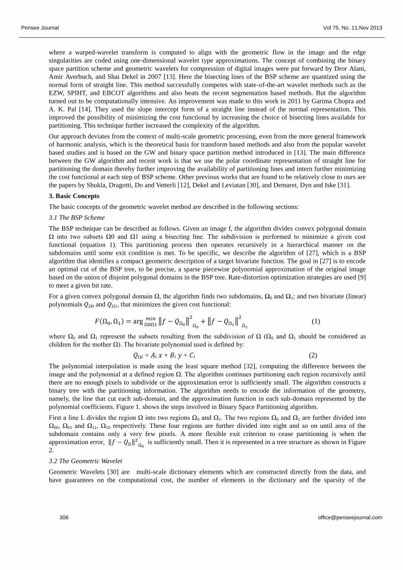
3. Basic Concepts

The basic concepts of the geometric wavelet method are described in the following sections:

3.1 The BSP Scheme

The BSP technique can be described as follows. Given an image f, the algorithm divides convex polygonal domain

Ω into two subsets Ω0 and Ω1 using a bisecting line. The subdivision is performed to minimize a given cost

functional (equation 1). This partitioning process then operates recursively in a hierarchical manner on the

subdomains until some exit condition is met. To be specific, we describe the algorithm of [27], which is a BSP

algorithm that identifies a compact geometric description of a target bivariate function. The goal in [27] is to encode

an optimal cut of the BSP tree, to be precise, a sparse piecewise polynomial approximation of the original image

based on the union of disjoint polygonal domains in the BSP tree. Rate-distortion optimization strategies are used [9]

to meet a given bit rate.

For a given convex polygonal domain Ω, the algorithm finds two subdomains, Ω0 and Ω1; and two bivariate (linear)

polynomials 𝑄Ω0 and 𝑄Ω1, that minimizes the given cost functional:

𝐹(Ω0, Ω1) = arg 𝑚𝑖𝑛Ω0Ω1

‖𝑓 − 𝑄Ω0‖

2

Ω0+ ‖𝑓 − 𝑄Ω1

‖2

Ω1 (1)

where Ω0 and Ω1 represent the subsets resulting from the subdivision of Ω (Ω0 and Ω1 should be considered as

children for the mother Ω). The bivariate polynomial used is defined by:

𝑄Ω𝑖 = 𝐴𝑖 𝑥 + 𝐵𝑖 𝑦 + 𝐶𝑖 (2)

The polynomial interpolation is made using the least square method [32], computing the difference between the

image and the polynomial at a defined region Ω. The algorithm continues partitioning each region recursively until

there are no enough pixels to subdivide or the approximation error is sufficiently small. The algorithm constructs a

binary tree with the partitioning information. The algorithm needs to encode the information of the geometry,

namely, the line that cut each sub-domain, and the approximation function in each sub-domain represented by the

polynomial coefficients. Figure 1. shows the steps involved in Binary Space Partitioning algorithm.

First a line L divides the region Ω into two regions Ω0 and Ω1. The two regions Ω0 and Ω1 are further divided into

Ω00, Ω01 and Ω11, Ω10 respectively. These four regions are further divided into eight and so on until area of the

subdomain contains only a very few pixels. A more flexible exit criterion to cease partitioning is when the

approximation error, ‖𝑓 − 𝑄Ω‖2Ω0

is sufficiently small. Then it is represented in a tree structure as shown in Figure

2.

3.2 The Geometric Wavelet

Geometric Wavelets [30] are multi-scale dictionary elements which are constructed directly from the data, and

have guarantees on the computational cost, the number of elements in the dictionary and the sparsity of the



representation. Geometric wavelets (GW) have been considered in context of image compression in [13]. It is a new

multi-scale data representation technique which is useful for a variety of applications such as data compression,

interpretation and anomaly detection [9]. The GW is defined as:

ΨΩ0 (𝑓) ≜ 1Ω0(QΩ0 − QΩ) (3)

Ω0 here means one of the children of mother, Ω. It is possible to reconstruct the function f using:

𝑓= ΣΩi ΨΩi (𝑓) (4)

Geometric Wavelet , ΨΩ is a “local difference” component that belongs to the detail space between two levels in the

BSP tree, a “low resolution” level associated with Ω and a “high resolution” level associated with Ω0. Geometric

wavelets also satisfy the vanishing moment property like isotropic wavelets [33], i.e., if f is locally a polynomial

over Ω, then minimizing of (1) gives QΩ0 = QΩ = 1, and therefore ΨΩ0 (𝑓) = 0. Unlike classical wavelets, geometric

wavelets do not satisfy the two scale relation and the biorthogonality property.

4. The GW Encoding Algorithm

As in wavelet decomposition, we only encode the differences between the original coarse projections of the data and

the points projected onto the planes at a finer scale, to find a compact representation for the data at the finer scale. In

order to do this, an effective scheme is developed based on the construction of a minimal space spanning this set of

differences. The axes of this difference space are termed “geometric wavelets”, and the projections of the finer-scale

corrections to the data points onto the plane spanned by these axes are called the “wavelet coefficients”. The process

is continued, forming a binary tree of mother and children at finer and finer scales until no further details are needed

to approximate the data up to a pre-specified accuracy. The process is discussed in detail in the following sections.

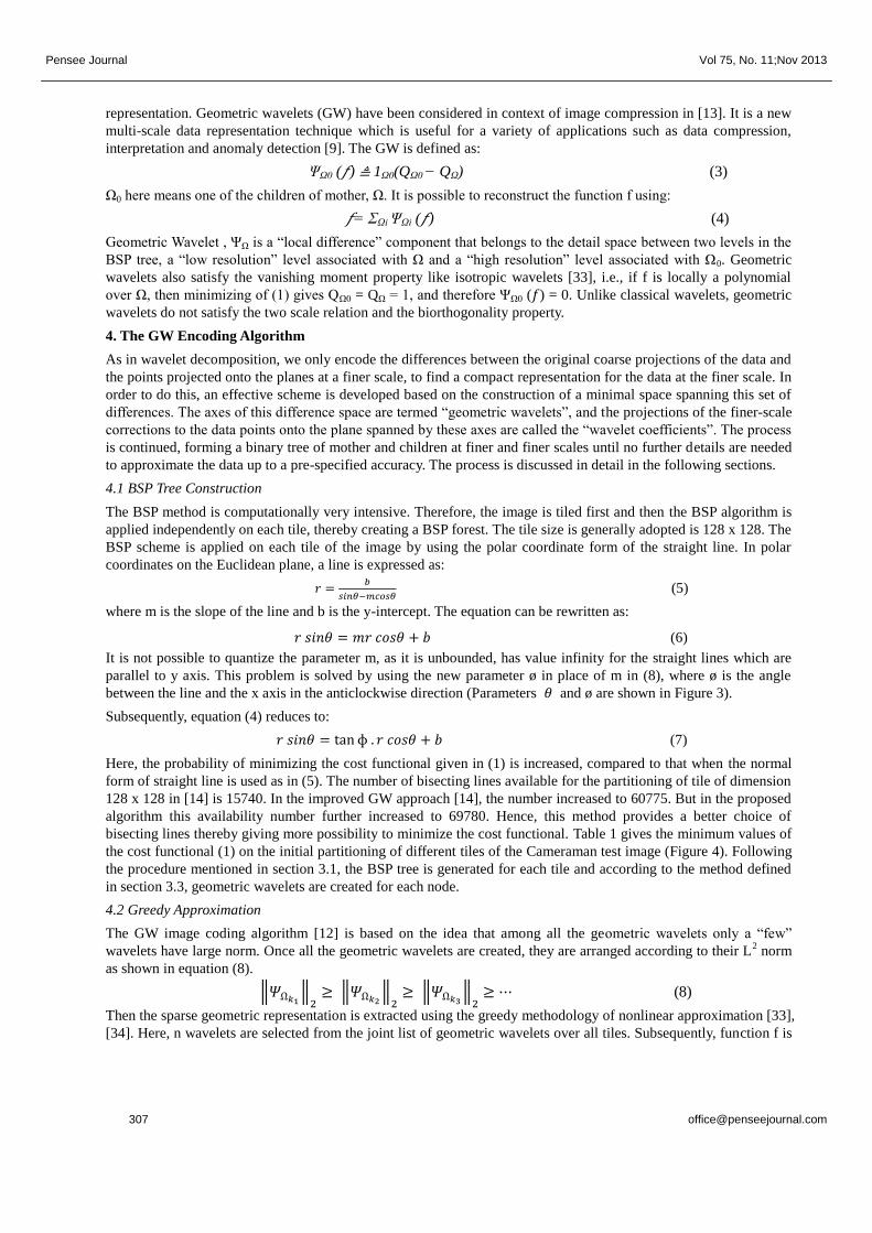
4.1 BSP Tree Construction

The BSP method is computationally very intensive. Therefore, the image is tiled first and then the BSP algorithm is

applied independently on each tile, thereby creating a BSP forest. The tile size is generally adopted is 128 x 128. The

BSP scheme is applied on each tile of the image by using the polar coordinate form of the straight line. In polar

coordinates on the Euclidean plane, a line is expressed as:

𝑟 =𝑏

𝑠𝑖𝑛𝜃−𝑚𝑐𝑜𝑠𝜃 (5)

where m is the slope of the line and b is the y-intercept. The equation can be rewritten as:

𝑟 𝑠𝑖𝑛𝜃 = 𝑚𝑟 𝑐𝑜𝑠𝜃 + 𝑏 (6)

It is not possible to quantize the parameter m, as it is unbounded, has value infinity for the straight lines which are

parallel to y axis. This problem is solved by using the new parameter ø in place of m in (8), where ø is the angle

between the line and the x axis in the anticlockwise direction (Parameters 𝜃 and ø are shown in Figure 3).

Subsequently, equation (4) reduces to:

𝑟 𝑠𝑖𝑛𝜃 = tan ɸ . 𝑟 𝑐𝑜𝑠𝜃 + 𝑏 (7)

Here, the probability of minimizing the cost functional given in (1) is increased, compared to that when the normal

form of straight line is used as in (5). The number of bisecting lines available for the partitioning of tile of dimension

128 x 128 in [14] is 15740. In the improved GW approach [14], the number increased to 60775. But in the proposed

algorithm this availability number further increased to 69780. Hence, this method provides a better choice of

bisecting lines thereby giving more possibility to minimize the cost functional. Table 1 gives the minimum values of

the cost functional (1) on the initial partitioning of different tiles of the Cameraman test image (Figure 4). Following

the procedure mentioned in section 3.1, the BSP tree is generated for each tile and according to the method defined

in section 3.3, geometric wavelets are created for each node.

4.2 Greedy Approximation

The GW image coding algorithm [12] is based on the idea that among all the geometric wavelets only a “few”

wavelets have large norm. Once all the geometric wavelets are created, they are arranged according to their L2 norm

as shown in equation (8).

‖𝛹Ω𝑘1‖

2≥ ‖𝛹Ω𝑘2

‖2

≥ ‖𝛹Ω𝑘3‖

2≥ ⋯ (8)

Then the sparse geometric representation is extracted using the greedy methodology of nonlinear approximation [33],

[34]. Here, n wavelets are selected from the joint list of geometric wavelets over all tiles. Subsequently, function f is



approximated using the n-term geometric wavelet sum given in equation (4), where n is the number of wavelets used

in the sparse representation.

4.3 Encoding

To obtain a reasonable approximation of the image, it is essential that if a child is present in the sparse representation,

then the mother should also be there, i.e, the BSP tree should be connected. Therefore, instead of encoding an n-term

tree approximation, we create an n + k geometric wavelet tree by considering more k nodes. The cost of imposing

the condition of the connected tree structure is not very huge, since there is high probability that if a child is

important all its ancestors are also important [33], [34]. The encoding of the geometry of the extracted connected

tree structure saves bits as only optimal cut is to be encoded.

There are two sorts of data to be encoded, 1) the geometry of the support of the wavelets participating in the sparse

representation and 2) the polynomial coefficients of the wavelet. Before encoding the extracted BSP forest, a small

header is written to the compressed file. Header consists of the minimum and maximum values of the coefficients of

the participating wavelet and the image graylevels. Out of header size of 26 bytes, 24 are used in the storage of the

minimum and the maximum values of the coefficients while 2 bytes are utilized to store the extremal values of the

image. “Root” geometric wavelets [14] contribute most in the approximation, so each root wavelet is encoded. The

encoding process is applied repeatedly for each of the geometric wavelet tree nodes in each tile.

4.3.1 Encoding the Geometry of the Support of the Wavelet

The following information is encoded for each of the participating node Ω:

• Number of children of Ω that participate in the sparse representation;

• In case only one child is participating, then whether it is the left or the right child;

• If Ω is not a leaf node, then the line that bisects Ω is encoded using the slope intercept form.

Left child and right child are defined as the sets of the pixels satisfying the inequality r - tan ø. r sinƟ <= b and r -

tan ø. r sinƟ >= b, respectively. The leaf node is encoded by using the bit “1.” Codes “00” and “01” are used for the

one child symbol and the two children symbol, respectively. If only 1 child of Ω is participating in the sparse

representation, then this event is encoded by using an additional bit. In case Ω is not a leaf node, then the indices of

the parameter ø and c of the bisecting line are encoded using the lossless variable length coding.

4.3.2 Encoding the Wavelet Coefficients

The coefficients of the wavelet polynomial, QΩ are quantized and encoded using an orthonormal representation of

П1(Ω), where П1(Ω) is the set of all bivariate linear polynomials over Ω. A bit allocation scheme for the coefficients

is applied using their distribution function (over all the domains) which is discussed in later sections. The “root”

wavelet of each tile is always encoded.

Quantizing the Wavelet Coefficients: To ensure the stability of the quantization process of the geometric wavelet

polynomial QΩ, we first need to find its representation in appropriate orthonormal basis. The orthonormal basis of

П1(Ω) is found using the standard Graham-Schmidt procedure. Let V1(x,y)=1, V2(x,y)=x, V3(x,y)=y and be the

standard polynomial basis. Then, an orthonormal basis of П1(Ω) is given by

𝑈1 =𝑉1

‖𝑉1‖

𝑈2 =𝑉2 − ⟨𝑉2,𝑈1⟩𝑈1

‖𝑉2 − ⟨𝑉2,𝑈1⟩𝑈1‖

𝑈3 =𝑉3 − ⟨𝑉3,𝑈1⟩𝑈1 − ⟨𝑉3,𝑈2⟩𝑈2

‖𝑉3 − ⟨𝑉3,𝑈1⟩𝑈1 − ⟨𝑉3,𝑈2⟩𝑈2‖ (9)

where inner product and norm are associated with the space L2 (Ω). Let

𝛹 = 𝛼𝑈1 + 𝛽𝑈2 + 𝛾𝑈3 (10)

be the representation of the geometric wavelet Ψ ϵ П1(Ω) in the orthonormal basis.

A bit allocation scheme is applied depending upon the distribution functions of the coefficients α, β and γ of the

wavelets participating in the sparse representation. Figure 5 shows the histogram of the wavelet coefficients of

Cameraman. Four bins are used to model the absolute value of the coefficients; bin limits are computed and passed



to the decoder. In case all the three coefficients of the wavelet are small, i.e., they are present in the bin containing

zero, then this event is encoded using single bit, but if any one of them is not small then the bin number of each

coefficient is encoded. After this quantized bits are written to the compressed file. Figures 6 and 7 show how the bit

budget allocation of Lena at the bit-rate 0.0625 bits per pixel (bpp) and 0.125 bpp is distributed among the GW

algorithm components respectively.

After the encoding step, a rate distortion optimization process [12] is carried out in order to attain the desired bit rate.

Pruning iterations [12] are applied, where at each iteration; the leaf node with minimal R-D slope is pruned until the

desired rate is accomplished.

5. Decoding

In the decoding stage, the compressed bit stream is read to find whether the participating node is a root node, has 1

child or 2 children, or a leaf node. If one child is participating then by using bit stream identification, it is found

whether it is left child or right child. If at least one of the children belongs to the sparse representation, then the

indexes of ø and b are decoded and using these index parameters ø and b of optimal cut are calculated. Thereafter,

using this optimal cut, domain is partitioned into two subdomains; and depending upon the situation vertex set of

only one child or both children is found. This process is repeated until entire bit stream is read.

6. Results and Discussion

The proposed algorithm is tested on the still image of Lena of bit depth 8 and of size 512x512. The implementation

is done using MATLAB. The Peak Signal to Noise Ratio (PSNR) based on Mean Square Error (MSE) is used as a

measure of “quality” [18]. MSE and PSNR are given by the following relations:

𝑀𝑆𝐸 =1

𝑚 x 𝑛∑ ∑ (𝑥𝑖,𝑗 − 𝑦𝑖,𝑗)2𝑛

𝑗=1𝑚𝑖=1 (11)

𝑃𝑆𝑁𝑅 = 10 log10 [(255)2

𝑀𝑆𝐸] (12)

where m x n is the image size, xi,j is the original image and yi,j is the reconstructed image. MSE and PSNR are

inversely proportional to each other and higher value of the PSNR implies better quality reconstructed image.

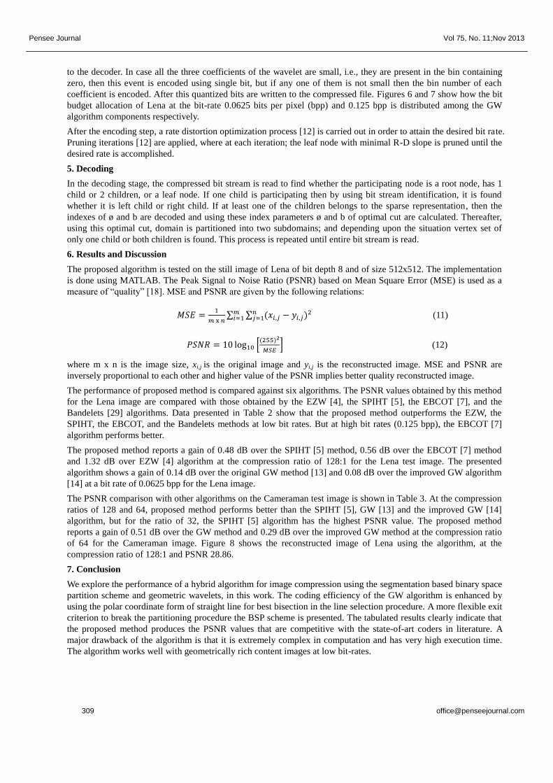
The performance of proposed method is compared against six algorithms. The PSNR values obtained by this method

for the Lena image are compared with those obtained by the EZW [4], the SPIHT [5], the EBCOT [7], and the

Bandelets [29] algorithms. Data presented in Table 2 show that the proposed method outperforms the EZW, the

SPIHT, the EBCOT, and the Bandelets methods at low bit rates. But at high bit rates (0.125 bpp), the EBCOT [7]

algorithm performs better.

The proposed method reports a gain of 0.48 dB over the SPIHT [5] method, 0.56 dB over the EBCOT [7] method

and 1.32 dB over EZW [4] algorithm at the compression ratio of 128:1 for the Lena test image. The presented

algorithm shows a gain of 0.14 dB over the original GW method [13] and 0.08 dB over the improved GW algorithm

[14] at a bit rate of 0.0625 bpp for the Lena image.

The PSNR comparison with other algorithms on the Cameraman test image is shown in Table 3. At the compression

ratios of 128 and 64, proposed method performs better than the SPIHT [5], GW [13] and the improved GW [14]

algorithm, but for the ratio of 32, the SPIHT [5] algorithm has the highest PSNR value. The proposed method

reports a gain of 0.51 dB over the GW method and 0.29 dB over the improved GW method at the compression ratio

of 64 for the Cameraman image. Figure 8 shows the reconstructed image of Lena using the algorithm, at the

compression ratio of 128:1 and PSNR 28.86.

7. Conclusion

We explore the performance of a hybrid algorithm for image compression using the segmentation based binary space

partition scheme and geometric wavelets, in this work. The coding efficiency of the GW algorithm is enhanced by

using the polar coordinate form of straight line for best bisection in the line selection procedure. A more flexible exit

criterion to break the partitioning procedure the BSP scheme is presented. The tabulated results clearly indicate that

the proposed method produces the PSNR values that are competitive with the state-of-art coders in literature. A

major drawback of the algorithm is that it is extremely complex in computation and has very high execution time.

The algorithm works well with geometrically rich content images at low bit-rates.



This research has thrown light into a new field of compression algorithms in terms of hybridization. However, our

results provide some weak evidence that show, hybrid techniques do help in improving the performance of image

coding algorithms. In future, further study of the issue may be done by combining the concepts of soft computing

techniques, especially the artificial neural networks and genetic algorithms with the geometric wavelets which may

help in reducing the time complexity of the algorithm. Probably, the design of new “geometric” context modelling

schemes combined with arithmetic encoding, may help in improving the performance of the algorithm. This study

can be further taken up by researchers in view of reduction in computational complexity and in turn time complexity

of the algorithm without compromising on the PSNR.

References

[1] Rao, K.R., and Yip, P. (1990). Discrete Cosine Transform: Algorithms, Advantages, Applications, New York:

Academic.

[2] Wallace, G. K. (1991). The JPEG Still-Picture Compression Standard, Commun. ACM, 34, 30-44.

[3] Daubechies, I. (1992). Ten Lectures on Wavelets, presented at the CBMS-NSF Reg. Conf. Ser. Applied

Mathematics.

[4] Shapiro, J. M. (1993). Embedded Image Coding Using Zerotrees of Wavelet Coefficients, IEEE Trans. Signal

Process., 41, 3445–3462.

[5] Said, A., and Pearlman, W. A. (1996). A New, Fast and Efficient Image Codec Based on Set Partioning in

Hierarchical Trees, IEEE Trans. Circuits Syst. Video Technol., 6, 243–250.

[6] Islam, A., and Pearlman, W. A. (1999). An Embedded and Efficient Low Complexity Hierarchical Image Coder,

in Proc. SPIE, 3653, 294–305.

[7] Tauban, D. (2000). High Performance Scalable Image Compression with EBCOT, IEEE Trans. Image Process.,

9, 1158–1170, (Jul. 2000).

[8] Skodras, A., Christopoulos, C., and Ebrahimi, T. (2001). The JPEG2000 Still Image Compression Standard,

IEEE Signal Process. Mag., 18, 36–58.

[9] Daubechies, I. (1990). The Wavelet Transform, Time Frequency Localization and Signal Analysis, IEEE Trans.

Inf. Theory, 36, 961–1005.

[10] Antonini, M., Barlaud, M., Mathieu, P., and Daubchies, I. (1992). Image Coding Using Wavelet Transform,

IEEE Trans. Image Process., 1, 205–220.

[11] Kunt, M., Ikonomopoulos, A., and Koche, M. (1985). Second Generation Image Coding Techniques, Proc.

IEEE, 73, 549–574.

[12] Shukla, R., Daragotti, P. L., Do, M. N., and Vetterli, M. (2005). Rate-Distortion Optimized Tree Structured

Compression Algorithms for Piecewise Polynomial Images, IEEE Trans. Image Process., 14, 343–359.

[13] Alani, D., Averbuch, A., and Dekel, S. (2007). Image Coding with Geometric Wavelets, IEEE Transactions on

Image Processing, 16, 69-77.

[14] Garima Chopra, & Pal, A., K. (2011). An Improved Image Compression Algorithm using Binary Space

Partition Scheme and Geometric Wavelets, IEEE Transactions on Image Processing, 20, 270 – 275.

[15] M., Kocher, and M., Kunt. (1982). A Contour-Texture Approach to Image Coding, in Proc. ICASSP, 436–440.

[16] G. J., Sullivan, and R. L., Baker. (1991). Efficient Quadtree Coding of Images and Video, in ICASSP Proc.,

2661-2664.

[17] M., Kunt, M., Benard, and R., Leonardi. (1987). Recent Results in High Compression Image Coding, IEEE

Trans. Circuits Syst., 34, 1306–1336.

[18] R., Leonardi and M., Kunt. (1985). Adaptive Split-and-Merge for Image Analysis and Coding, Proc. SPIE, 594.

[19] A. N., Netravali and B. G., Haskell. (1988). Digital Pictures: Representations and Compressions, New York:

Plenum.

[20] J., Froment and S., Mallat. (1992). Wavelets: A Tutorial in Theory and Applications, C. K. Chui, Ed. Academic

Press, New York, Second Generation Compact Image Coding with Wavelets



[21] E., Candes and D., Donoho. (2001). Curvelets and Curvilinear Integrals, Journal of Approximation Theory, 113,

59–90.

[22] A., Cohen and B., Matei. (2001). Compact Representations of Images by Edge Adapted Multiscale

Transforms, Proceedings of the IEEE ICIP Conference, Thessaloniki.

[23] R. L., Claypoole, G. M., Davis, W., Sweldens, and R. G. (2003). Baraniuk, Nonlinear Wavelet Transforms for

Image Coding via Lifting, IEEE Trans. Image Process., 12, 1449–1459.

[24] M. N., Do and M., Vetterli. (2005). The Contourlet Transform: An Efficient Directional Multiresolution Image

Representation, IEEE Trans. Image Process., 14, 2091–2106.

[25] M. N., Do and Yue Lu. (2006). A New Contourlet Transform with Sharp Frequency Localization, IEEE

International Conference on Image Processing, 1629–1632.

[26] M. S., Paterson and F. F., Yao. (1990). Efficient Binary Space Partitions for Hidden-Surface Removal and Solid

Modeling, Discrete Comput. Geom., 5, 485–503.

[27] H., Radha, M., Vetterli, and R., Leonardi. (1996). “Image Compression Using Binary Space Partitioning Trees”,

IEEE Trans. Image Process., 5, pp. 1610–1624.

[28] P., Salembier and L., Garrido. (2000). Binary Partition Tree as an Efficient Representation for Image

Processing, Segmentation, and Information Retrieval, IEEE Trans. Image Process., 9, 561–576.

[29] E. L., Pennec and S., Mallat. (2005). Sparse Geometric Image Representation with Bandelets, IEEE Trans.

Image Process., 14, 423–438.

[30] Dekel, and Leviatan. (2005). Adaptive Multivariate Approximation Using Binary Space Partitions and

Geometric Wavelets, SIAM journal on Numerical Analysis, 43, 707–732.

[31] L., Demaret, N., Dyn, and Iske, A. (1990). Image Compression by Linear Splines Over Adaptive Triangulations,

[Online]. Available: citeseer.ist.psu.edu/646599.html

[32] H., Radha. (1990). Least-Square Binary Partitioning of LZ Functions with Convex Domains, AT&T Bell Labs.

Tech. Memo, Draft.

[33] R., DeVore. (1998). Nonlinear Approximation, Acta Numer., 7, 51–150.

[34] V. N., Temlyakov. (2003). Nonlinear methods of approximation, Found. Comput. Math., 3, 33–107.

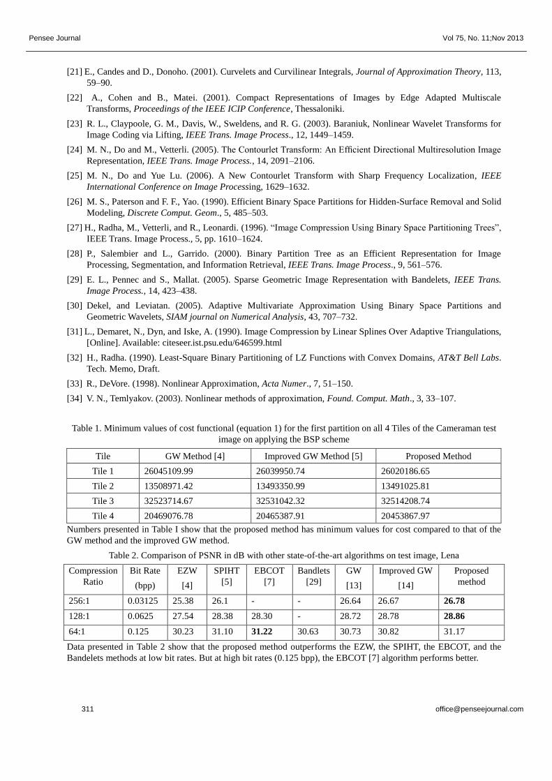
Table 1. Minimum values of cost functional (equation 1) for the first partition on all 4 Tiles of the Cameraman test

image on applying the BSP scheme

Tile GW Method [4] Improved GW Method [5] Proposed Method

Tile 1 26045109.99 26039950.74 26020186.65

Tile 2 13508971.42 13493350.99 13491025.81

Tile 3 32523714.67 32531042.32 32514208.74

Tile 4 20469076.78 20465387.91 20453867.97

Numbers presented in Table I show that the proposed method has minimum values for cost compared to that of the

GW method and the improved GW method.

Table 2. Comparison of PSNR in dB with other state-of-the-art algorithms on test image, Lena

Compression

Ratio

Bit Rate

(bpp)

EZW

[4]

SPIHT

[5]

EBCOT

[7]

Bandlets

[29]

GW

[13]

Improved GW

[14]

Proposed

method

256:1 0.03125 25.38 26.1 - - 26.64 26.67 26.78

128:1 0.0625 27.54 28.38 28.30 - 28.72 28.78 28.86

64:1 0.125 30.23 31.10 31.22 30.63 30.73 30.82 31.17

Data presented in Table 2 show that the proposed method outperforms the EZW, the SPIHT, the EBCOT, and the

Bandelets methods at low bit rates. But at high bit rates (0.125 bpp), the EBCOT [7] algorithm performs better.



Table 3. Comparison of PSNR in dB with other state-of-the-art algorithms on Cameraman test image

Compression

Ratio

Bit Rate

(bpp)

SPIHT

[5]

GW

[13]

Improved GW

[14]

Proposed

method

128:1 0.0625 22.8 22.93 23.04 23.74

64:1 0.125 25 25.07 25.29 25.58

32:1 0.25 28 27.48 27.62 27.82

At the compression ratios of 128 and 64, proposed method performs better than the SPIHT [5], GW [13] and the

improved GW [14] algorithm, but for the ratio of 32, the SPIHT [5] algorithm has the highest PSNR value. The

proposed method reports a gain of 0.51 dB over the GW method and 0.29 dB over the improved GW method at the

compression ratio of 64 for the Cameraman image.

Figure 1. Binary Space Partitioning of the domain Ω (two levels).

Figure 1. shows the steps involved in Binary Space Partitioning algorithm. First a line L divides the region Ω into

two regions Ω0 and Ω1. The two regions Ω0 and Ω1 are further divided into Ω00, Ω01 and Ω11, Ω10 respectively. These

four regions are further divided into eight and so on until area of the subdomain contains only a very few pixels. A

more flexible exit criterion to cease partitioning is when the approximation error, ‖𝑓 − 𝑄Ω‖2Ω0

is sufficiently small.

Then it is represented in a tree structure as shown in Figure 2.

Figure 2. BSP tree representation of the polygon in Figure 1.



Figure 3. Partition of the image domain into two subdomains - Parameters θ and ɸ

Figure 4. Tiling of Cameraman image (Tile size 128x128)

Figure 5. Histogram of wavelet coefficients, α (left), β (middle) and γ (right) of Cameraman image.

We can infer from the graph that there is a very high probability for the coefficients α, β and γ to be small (the graph

resembles a generalized-Gaussian function).

Figure 6. Bit budget allocation for Cameraman at bit-rate, 0.0625 bpp. Output file size is 4 KBytes

3219, 76.78%

618, 14.7%

291, 6.94% 64, 1.5%

Polynomials

Tree Structure

Bisecting Lines

Header



Figure 7. Bit budget allocation for Cameraman at bit-rate, 0.125 bpp. Output file size is 8 KBytes.

The charts show the bit budget allocation of Lena test image at different bit-rates. It can be inferred from the charts

that at higher bit-rates, the bit budget for the polynomial coefficients relatively increases, while the bit allocation for

the bisecting lines decreases.

Figure 8. Top Left: Original Lena. (512 x 512). Top Center: Reconstructed Lena using the GW algorithm, 0.0625

bpp, PSNR=28.72. Top Right: Reconstructed Lena using the proposed method, 0.0625 bpp, PSNR=28.86. Bottom

Left: Original Cameraman. (256 x 256). Bottom Center: Reconstructed Cameraman using the GW algorithm, 0.0625

bpp, PSNR=22.93. Bottom Right: Reconstructed Lena using the proposed method, 0.0625 bpp, PSNR=23.74.

6631, 80.94%

428, 5.2%

1007, 12.5% 114, 1.3%

Polynomials

Tree Structure

Bisecting Lines

Header

A Superior Hybrid Algorithm Based on Geometric Wavelets for Compression of Digital Images

Documents