A Study on Transmit Precoder Designs for Spatial Modulation and Deep Learning-Based Beam Allocation by Yuwen Cao Dissertation Submitted by Yuwen Cao In Partial Fulfillment of the Requirements for the Degree of Ph.D. in Engineering Supervisor: Prof. Tomoaki Ohtsuki, Ph.D. August, 2021 Graduate School of Science and Technology Keio University

Welcome message from author
This document is posted to help you gain knowledge. Please leave a comment to let me know what you think about it! Share it to your friends and learn new things together.
Transcript

A Study on Transmit Precoder Designs for SpatialModulation and Deep Learning-Based Beam Allocation
by
Yuwen Cao
DissertationSubmitted by Yuwen Cao
In Partial Fulfillment of the Requirements for the Degree of
Ph.D. in Engineering
Supervisor: Prof. Tomoaki Ohtsuki, Ph.D.
August, 2021
Graduate School of Science and TechnologyKeio University

Contents
List of Tables . . . . . . . . . . . . . . . . . . . . . . . . . . . . . . . . . . . . . v
List of Figures . . . . . . . . . . . . . . . . . . . . . . . . . . . . . . . . . . . . vi
Abstract . . . . . . . . . . . . . . . . . . . . . . . . . . . . . . . . . . . . . . . . viii
Acknowledgments . . . . . . . . . . . . . . . . . . . . . . . . . . . . . . . . . . x
1 Introduction . . . . . . . . . . . . . . . . . . . . . . . . . . . . . . . . . . . 11.1 Research Background . . . . . . . . . . . . . . . . . . . . . . . . . . . . 2
1.2 Precoding in 5G . . . . . . . . . . . . . . . . . . . . . . . . . . . . . . . 3
1.2.1 Precoder Design and Application . . . . . . . . . . . . . . . . . 3
1.2.2 Deep Learning-Based Precoder Design . . . . . . . . . . . . . . 4
1.3 Scope and Contributions of the Dissertation . . . . . . . . . . . . . . . . 4
1.3.1 Scope of the Dissertation . . . . . . . . . . . . . . . . . . . . . . 4
1.3.2 Summary of the Dissertation . . . . . . . . . . . . . . . . . . . . 6
1.3.3 Contributions of the Dissertation . . . . . . . . . . . . . . . . . . 11
2 Non-Convex Precoding Optimization Problem . . . . . . . . . . . . . . . . 132.1 Introduction . . . . . . . . . . . . . . . . . . . . . . . . . . . . . . . . . 14
2.2 Transmit Precoding Design Problem . . . . . . . . . . . . . . . . . . . . 14
2.2.1 Problem Statement . . . . . . . . . . . . . . . . . . . . . . . . . 14
2.2.2 Problem Analysis . . . . . . . . . . . . . . . . . . . . . . . . . . 15
2.3 Joint Precoding Weight Optimization and Power Allocation Problem . . . 16
2.3.1 Problem Statement . . . . . . . . . . . . . . . . . . . . . . . . . 16
2.3.2 Challenges . . . . . . . . . . . . . . . . . . . . . . . . . . . . . 17
2.3.3 Conventional Approaches . . . . . . . . . . . . . . . . . . . . . 18
2.4 Conclusion of this Chapter . . . . . . . . . . . . . . . . . . . . . . . . . 18
3 GPSM: Orthogonality Structure Design . . . . . . . . . . . . . . . . . . . . 193.1 Introduction . . . . . . . . . . . . . . . . . . . . . . . . . . . . . . . . . 20
3.2 System Model . . . . . . . . . . . . . . . . . . . . . . . . . . . . . . . . 21
ii

3.2.1 Design of GPSM Symbols . . . . . . . . . . . . . . . . . . . . . 213.2.2 Precoding Design . . . . . . . . . . . . . . . . . . . . . . . . . . 223.2.3 Channel Correlation Modeling . . . . . . . . . . . . . . . . . . . 22
3.3 Optimization of The RAS Selection . . . . . . . . . . . . . . . . . . . . 243.3.1 The RAS Selection Criterion . . . . . . . . . . . . . . . . . . . . 24
3.4 Orthogonality Structure Designs for GPSM . . . . . . . . . . . . . . . . 253.4.1 Orthogonality Structure Designs . . . . . . . . . . . . . . . . . . 253.4.2 OSD-Aided Receive Antenna Subset Selection . . . . . . . . . . 27
3.5 Analysis and Discussion of the Results . . . . . . . . . . . . . . . . . . . 283.5.1 Observations . . . . . . . . . . . . . . . . . . . . . . . . . . . . 28
3.6 Conclusion of This Chapter . . . . . . . . . . . . . . . . . . . . . . . . . 30
4 Dual-Ascent Inspired Transmit Precoding: Design & Application . . . . . . 314.1 Introduction . . . . . . . . . . . . . . . . . . . . . . . . . . . . . . . . . 324.2 Motivations . . . . . . . . . . . . . . . . . . . . . . . . . . . . . . . . . 33
4.2.1 Spatial Modulation . . . . . . . . . . . . . . . . . . . . . . . . . 334.2.2 Related Work . . . . . . . . . . . . . . . . . . . . . . . . . . . . 344.2.3 Our Idea . . . . . . . . . . . . . . . . . . . . . . . . . . . . . . 34
4.3 System Model . . . . . . . . . . . . . . . . . . . . . . . . . . . . . . . . 344.3.1 Maximum-Likelihood Detection . . . . . . . . . . . . . . . . . . 364.3.2 Solutions for The Introduced MMD Problem . . . . . . . . . . . 374.3.3 Discussion . . . . . . . . . . . . . . . . . . . . . . . . . . . . . 38
4.4 Problem Statement . . . . . . . . . . . . . . . . . . . . . . . . . . . . . 384.4.1 Discussion . . . . . . . . . . . . . . . . . . . . . . . . . . . . . 384.4.2 Problem Transformation . . . . . . . . . . . . . . . . . . . . . . 39
4.5 Proposed Approach . . . . . . . . . . . . . . . . . . . . . . . . . . . . . 394.5.1 The BFGS-Aided Dual-Ascent Approach . . . . . . . . . . . . . 394.5.2 Discussion . . . . . . . . . . . . . . . . . . . . . . . . . . . . . 434.5.3 Complexity Analysis . . . . . . . . . . . . . . . . . . . . . . . . 45
4.6 Experimental Results . . . . . . . . . . . . . . . . . . . . . . . . . . . . 464.6.1 BER Performance Evaluations . . . . . . . . . . . . . . . . . . . 46
4.7 Conclusion of This Chapter . . . . . . . . . . . . . . . . . . . . . . . . . 47
5 Beam and Power Allocation Using Deep Learning . . . . . . . . . . . . . . 495.1 Introduction . . . . . . . . . . . . . . . . . . . . . . . . . . . . . . . . . 505.2 Data . . . . . . . . . . . . . . . . . . . . . . . . . . . . . . . . . . . . . 51
5.2.1 Realistic Channel Generation . . . . . . . . . . . . . . . . . . . 515.2.2 Simulation Specification . . . . . . . . . . . . . . . . . . . . . . 51
5.3 System Model . . . . . . . . . . . . . . . . . . . . . . . . . . . . . . . . 525.3.1 Channel Model . . . . . . . . . . . . . . . . . . . . . . . . . . . 53
iii

5.3.2 Beamforming Weights . . . . . . . . . . . . . . . . . . . . . . . 535.3.3 Downlink Beam Broadcasting . . . . . . . . . . . . . . . . . . . 54
5.4 Problem Statement . . . . . . . . . . . . . . . . . . . . . . . . . . . . . 555.4.1 Sum-Rate Maximization Problem . . . . . . . . . . . . . . . . . 555.4.2 Problem Transformation . . . . . . . . . . . . . . . . . . . . . . 55
5.5 High-Resolution Beam-Quality Prediction . . . . . . . . . . . . . . . . . 565.5.1 Beam-Quality Prediction Module . . . . . . . . . . . . . . . . . 56
5.6 Proposed Beam and Power Allocation . . . . . . . . . . . . . . . . . . . 585.6.1 Optimal Allocation Solution . . . . . . . . . . . . . . . . . . . . 585.6.2 Deep Learning-Based Allocation Solution . . . . . . . . . . . . . 60
5.7 Experimental Results . . . . . . . . . . . . . . . . . . . . . . . . . . . . 625.7.1 Performance Metrics . . . . . . . . . . . . . . . . . . . . . . . . 625.7.2 Accuracy Analysis . . . . . . . . . . . . . . . . . . . . . . . . . 625.7.3 Sum-Rate Performance . . . . . . . . . . . . . . . . . . . . . . . 635.7.4 Beam Confliction Probability . . . . . . . . . . . . . . . . . . . 64
5.8 Conclusion of This Chapter . . . . . . . . . . . . . . . . . . . . . . . . . 65
6 Conclusions and Future Work . . . . . . . . . . . . . . . . . . . . . . . . . 676.1 Conclusions . . . . . . . . . . . . . . . . . . . . . . . . . . . . . . . . . 686.2 Future Work . . . . . . . . . . . . . . . . . . . . . . . . . . . . . . . . . 69
Appendix A List of Author’s Publications and Awards . . . . . . . . . . . . . . 71A.1 Journals . . . . . . . . . . . . . . . . . . . . . . . . . . . . . . . . . . . 71A.2 Full Articles on International Conferences Proceedings . . . . . . . . . . 72A.3 Articles on Domestic Conference Proceedings . . . . . . . . . . . . . . . 72A.4 Technical Reports . . . . . . . . . . . . . . . . . . . . . . . . . . . . . . 72
References . . . . . . . . . . . . . . . . . . . . . . . . . . . . . . . . . . . . . . 75
iv

List of Tables
3.1List of Commonly Used Functions and Notations. . . . . . . . . . . . . . . . . . 21
3.2The simulation parameter setting. . . . . . . . . . . . . . . . . . . . . . . . . 28
4.1List of Commonly Used Functions and Notations. . . . . . . . . . . . . . . . . . 33
4.2 Complexity Comparisons Among Different Precoding Schemes . . . . . . . . . . . 454.3 Operation Number Comparisons for Different Precoding Schemes in Single-/Multi-User
Scenarios . . . . . . . . . . . . . . . . . . . . . . . . . . . . . . . . . . . 464.4
The simulation parameter setting. . . . . . . . . . . . . . . . . . . . . . . . . 47
5.1List of Commonly Used Functions and Notations. . . . . . . . . . . . . . . . . . 51
5.2The Beam Confliction Probability for mmWave Multiuser System with Typical mmWave
Settings . . . . . . . . . . . . . . . . . . . . . . . . . . . . . . . . . . . . 605.3
The Simulation Parameter Setting. . . . . . . . . . . . . . . . . . . . . . . . . 62
v

List of Figures
1.1 The scope of this dissertation. . . . . . . . . . . . . . . . . . . . . . . . 5
1.2 An overview of this dissertation. . . . . . . . . . . . . . . . . . . . . . . 7
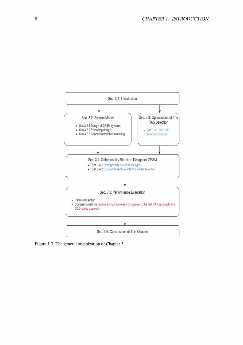
1.3 The general organization of Chapter 3. . . . . . . . . . . . . . . . . . . . 8
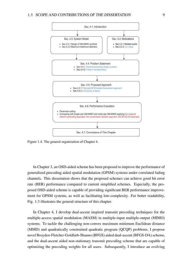
1.4 The general organization of Chapter 4. . . . . . . . . . . . . . . . . . . . 9
1.5 The general organization of Chapter 5. . . . . . . . . . . . . . . . . . . . 10
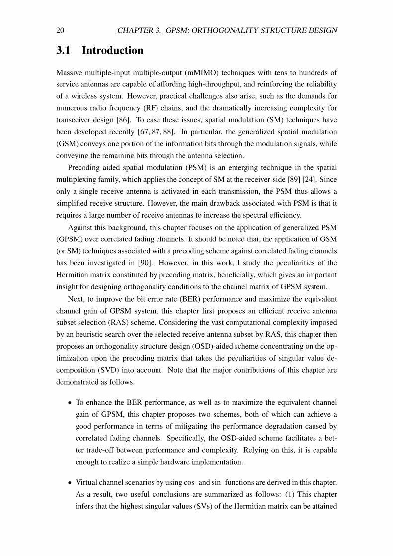
3.1 BER performance comparisons among the conventional PSM systems forthe scenario of various transceiver antenna configurations, ρ = 0, na = 1,4-QAM (M = 4), and 64-QAM (M = 64). . . . . . . . . . . . . . . . . . 23
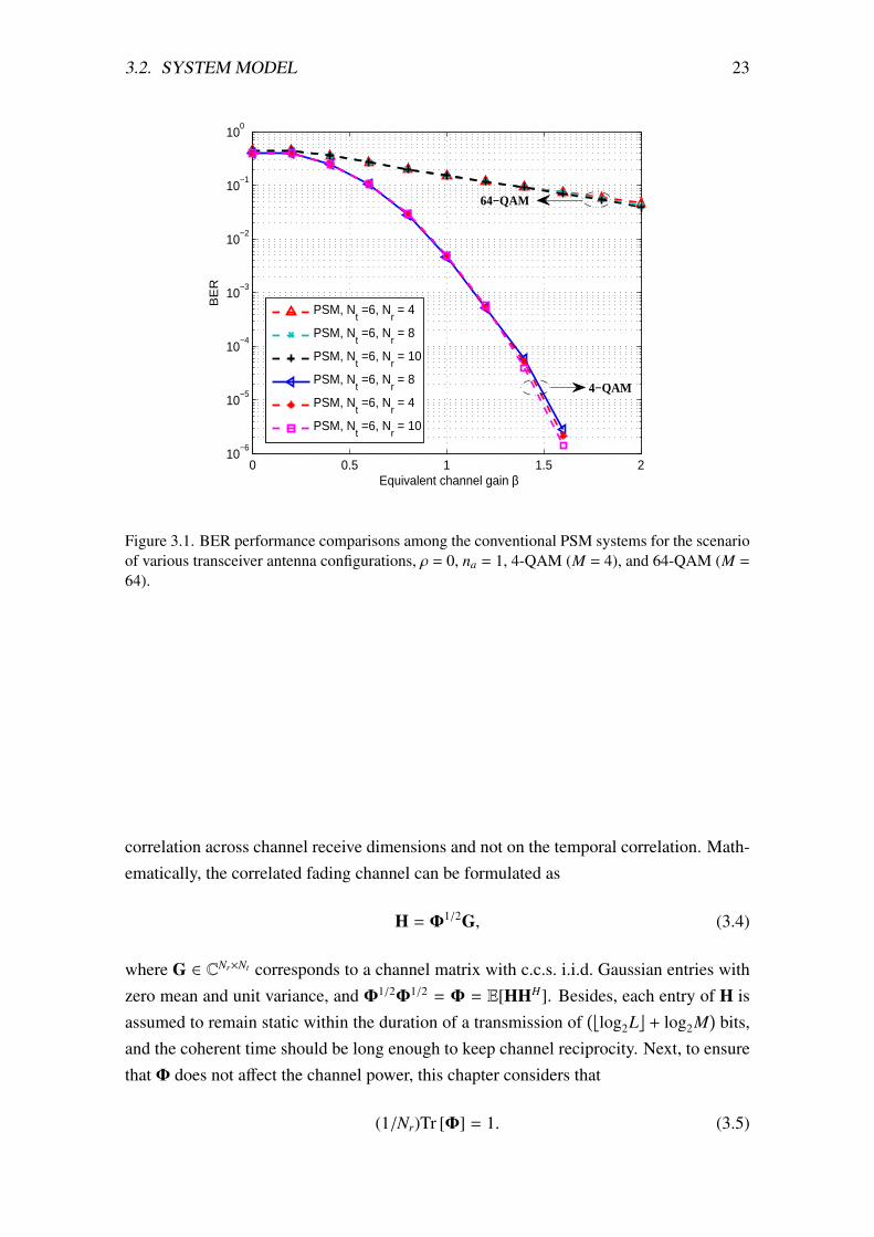
3.2 An overview of the RAS selection. . . . . . . . . . . . . . . . . . . . . . 25
3.3 The BERs of fast RAS, OSD-aided scheme, and optimal scheme for G-PSM and PSM systems with Nt = 3, Nr = 6, exponential correlation pa-rameter |ρ| = 0.5 or 0, na = 2, and 4-QAM. . . . . . . . . . . . . . . . . . 29
3.4 The BERs of fast RAS, OSD-aided scheme, and optimal scheme for G-PSM and PSM with Nt = 3, Nr = 6, exponential correlation parameter |ρ|= 0.5 or 0, na = 2, and 32-QAM. . . . . . . . . . . . . . . . . . . . . . . 29
4.1 Minimum ED dmin versus the quantized phase angle θq and the quantizedpower modulus pq. (a) θq = 0, Nt = Nr = 5, K = 1, and L1 = 8; (b) Nt =
Nr = 5, K = 1, and L2 = 4. . . . . . . . . . . . . . . . . . . . . . . . . . 37
4.2 The BERs of the TAC, the diagonal TPC, the CI, and the proposed BFGS-DA schemes for single-user SM-MIMO and MASM-MIMO systems withNt1 = 8, K = 1, Nr = 2 or 4, and M = 4. . . . . . . . . . . . . . . . . . . 48
4.3 The BERs of the diagonal TPC, the TAC, the CI, and the proposed BFGS-DA schemes for multi-user SM-MIMO and MASM-MIMO, as well asGSM-MIMO with Nt1 = Nt2 = 8, K = 2, Nr = 4, and M = 4. . . . . . . . . 48
5.1 The simulation environment in the ray tracing simulator. . . . . . . . . . 52
5.2 The simulation setting of the wireless insite simulator. . . . . . . . . . . . 52
5.3 The propagation paths for receivers. . . . . . . . . . . . . . . . . . . . . 53
vi
5.4 An overview of the beam-image dataset generation and high resolutionbeam-quality image prediction framework. Note that only a portion ofs beam images are combined into a time-sequential image to reduce thetraining overhead. Besides,
√mtx ×
√mtx
(√Mtx ×
√Mtx
)represents the
dimension of the low (high) resolution beam image; hereby Mtx and mtx
are assumed to be 64 and 16, respectively. . . . . . . . . . . . . . . . . . 575.5 High-resolution beam-quality image prediction module. . . . . . . . . . . 585.6 Prediction accuracy of our beam-quality prediction module employing the
3D Conv-LSTM architecture under various hyperparameter s = {1, 2, 3}. . 635.7 Test accuracy of our beam-quality prediction module employing the 3D
Conv-LSTM architecture under various hyperparameter s = {1, 2, 3}. . . . 635.8 MSE performance of our beam-quality prediction scheme employing the
CNN, 3D Conv-GRU, and 3D Conv-LSTM architectures under varioushyperparameter s = {1, 2, 3}. . . . . . . . . . . . . . . . . . . . . . . . . 64
5.9 Sum-rate performance of the optimal allocation (Alg. 1), the random al-location, and the deep learning-based approach (Alg. 2) with K = {4, 6},m = {6, 10}. . . . . . . . . . . . . . . . . . . . . . . . . . . . . . . . . . 64
5.10 The beam confliction probability of the top-m selection approach withdistinct (m, γ) configurations and K = 16. . . . . . . . . . . . . . . . . . 65
vii

A Study on Transmit Precoder Designs for SpatialModulation and Deep Learning-Based Beam Allocation
Yuwen [email protected].
Keio University, 2021
Supervisor: Prof. Tomoaki Ohtsuki, [email protected]
Abstract
In this dissertation, I investigate the transmit precoder designs for spatial modulation(SM) and deep learning-based high-resolution beam-quality prediction for guaranteeinghigh-quality and low-latency communications. Notably, the system performances de-grade significantly caused by the correlated fading channels. To tackle this challenge,I first introduce an orthogonality structure design (OSD) for the generalized precodingaided spatial modulation (GPSM) to overcome the performance degradation. To facil-itate a better trade-off between performance and computational complexity, I study thepeculiarities of the Hermitian matrix which provides an important insight for conceivingorthogonality conditions to the channel matrix of GPSM system. Next, I observe thatthe system performances degrade distinctly when employing the current existing trans-mit precoding (TPC) approaches into the multiple-access spatial modulation (MASM)in multiple-input multiple-output (MIMO) systems. To address this challenge, I nex-t investigate the dual-ascent inspired TPC algorithms for MASM-MIMO systems. Inaddition, I study the peculiarities of the convex optimization methods that take the dual-ascent method into account to find a global optimum against the non-convex maximumminimum Euclidean distance (MMD) and quadratically constrained quadratic program(QCQP) problems, as well as to enlarge the energy-efficiency. Numerical results showthe benefits of our proposals under different kinds of performance metrics. On the otherhand, due to the challenges in mmWave networks that: (i) existing deep-learning basedapproaches predict the beamforming matrix that in practice can not be well-suited to theunderlying channel distribution as the beamforming dimension at BS is large; (ii) userequipments (UEs) who are geographically co-located together may render the serve beamconflicts, thus deteriorating the system performance. In this context, to make fast beam-forming available at BS, this dissertation focuses on investigating the deep learning-basedbeam and power allocation by exploiting the image super-resolution technology. More
viii

explicitly, this dissertation develops a deep learning-based beam and power resource allo-cation approach which can accurately allocate the desired beam and power for UEs withlow-overhead. Numerical results verify the effectiveness of our approach.
The reminder of this dissertation will be structured as follows:Chapter 1 introduces the concept of transmit precoding, and its applications into the
MASM-MIMO systems. Besides, high resolution beam quality prediction in the downlinkmmWave communication and its challenges are also introduced in this chapter. Severalrelated works in reference to the above two research topics are also introduced.
Chapter 2 introduces non-convex precoding optimization problem as well as the analy-sis of the non-convex problem solver and its challenges. In particular, this dissertation fo-cuses on investigating two non-convex optimization problems, i.e., the transmit-precodingoptimization problem and the joint precoding weight optimization and power allocationproblem.
Chapter 3 develops a low-complexity solution to the non-convex precoding optimiza-tion problem. In addition, this dissertation introduces an OSD for the GPSM to overcomethe performance degradation.
Chapter 4 studies the challenging non-convex MMD problem and the non-convexQCQP problem. To develop an efficient solution to the above problems as well as to keeplow hardware realization cost, this dissertation presents a dual-ascent inspired transmitprecoding approach by exploiting the primal-dual optimality theory.
Chapter 5 introduces a low-overhead beam and power allocation solution as a solver tothe non-convex joint beamforming (precoding) weight optimization and power allocationproblem. By exploiting the deep learning technology and the super resolution technology,high-resolution beam-quality prediction with high accuracy can be realized with a low-overhead.
Finally, Chapter 6 concludes this dissertation by making remark on the key technolo-gies proposed by Chapter 3, Chapter 4, and Chapter 5 as well as stating their technicalcontributions. Besides, Chapter 6 presents possible venues for future research topic ondeveloping low overhead beamforming (precoding) weight prediction and applications.
ix

Acknowledgments
Firstly, I would like to thank my supervisor Prof. Tomoaki Ohtsuki for giving me fir-m and continuous support and encouragement which helps me much during my Ph.D.period. Under the guidance of Prof. Tomoaki Ohtsuki, I learn much about how to doresearch project and how to upgrade and improve oneself, as well as how to be a scientificresearcher. Without Ohtsuki Sensei’s great support and motivation, this Ph.D. degree willnot be achievable. I am very appreciative of Ohtsuki Sensei’s step-by-step guidance forcompleting this dissertation. I addition, I would love to thank Ohtsuki Sensei for carefullyrevising my academic journal and conference papers.
Next, I am also very appreciative of the committee members, Prof. Sasase, Prof.Sanada, and Prof. Gui who raise very helpful comments and suggestions for improvingthe technical and written quality of this dissertation.
I would also like to express my thanks to all the Ohtsuki Lab members, especiallySiyuan Yang, Mondher Bouazizi, Kohei Yamamoto, Junta Tachibana, and Yuva Kumarwho have always been there for me, and gave me tremendous assistance not only in myresearch but also the daily life of studying abroad. In particular, I would like to thankAssistant Professor Mondher Bouazizi who gave me a help on my python code.
I would also like to say a heartfelt thank you to my parents, my grandfather, my youngbrother Shaoji Cao, my young sister Yiyi Cao, who always encourage me and keep meenthusiastic and looking forward to overcome difficulties and complete research projectsduring this period.
Yuwen Cao
x

Chapter 1
Introduction
1
2 CHAPTER 1. INTRODUCTION
This dissertation consists of two research topics. The first topic is to tackle challeng-ing non-convex precoding optimization and application problems in spatial modulation.The second one is how to make use of the deep learning techniques to predict the pre-coding weights and apply the predicted precoder into multiuser mmWave networks. Iwould like to kindly note that both the optimization-based precoding (in first topic) andthe deep learning-based precoding (in second topic) can guarantee system performanceimprovement while enjoying a low-complexity merit. However, the research direction ofthe optimization-based precoding and the deep learning-based precoding is different ingeneral.
1.1 Research Background
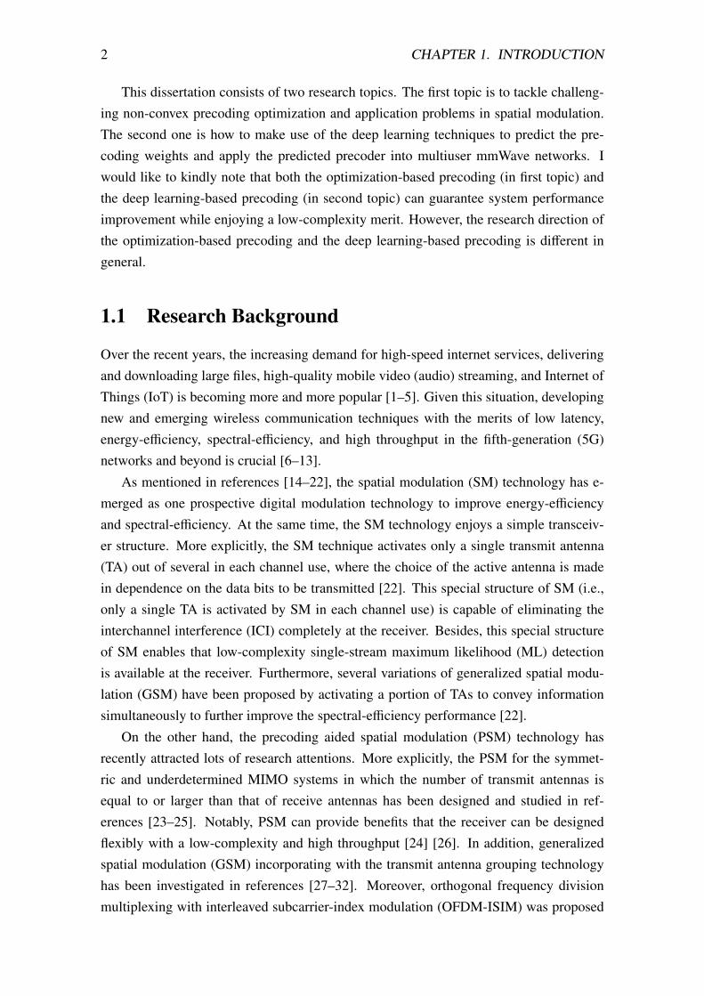
Over the recent years, the increasing demand for high-speed internet services, deliveringand downloading large files, high-quality mobile video (audio) streaming, and Internet ofThings (IoT) is becoming more and more popular [1–5]. Given this situation, developingnew and emerging wireless communication techniques with the merits of low latency,energy-efficiency, spectral-efficiency, and high throughput in the fifth-generation (5G)networks and beyond is crucial [6–13].
As mentioned in references [14–22], the spatial modulation (SM) technology has e-merged as one prospective digital modulation technology to improve energy-efficiencyand spectral-efficiency. At the same time, the SM technology enjoys a simple transceiv-er structure. More explicitly, the SM technique activates only a single transmit antenna(TA) out of several in each channel use, where the choice of the active antenna is madein dependence on the data bits to be transmitted [22]. This special structure of SM (i.e.,only a single TA is activated by SM in each channel use) is capable of eliminating theinterchannel interference (ICI) completely at the receiver. Besides, this special structureof SM enables that low-complexity single-stream maximum likelihood (ML) detectionis available at the receiver. Furthermore, several variations of generalized spatial modu-lation (GSM) have been proposed by activating a portion of TAs to convey informationsimultaneously to further improve the spectral-efficiency performance [22].
On the other hand, the precoding aided spatial modulation (PSM) technology hasrecently attracted lots of research attentions. More explicitly, the PSM for the symmet-ric and underdetermined MIMO systems in which the number of transmit antennas isequal to or larger than that of receive antennas has been designed and studied in ref-erences [23–25]. Notably, PSM can provide benefits that the receiver can be designedflexibly with a low-complexity and high throughput [24] [26]. In addition, generalizedspatial modulation (GSM) incorporating with the transmit antenna grouping technologyhas been investigated in references [27–32]. Moreover, orthogonal frequency divisionmultiplexing with interleaved subcarrier-index modulation (OFDM-ISIM) was proposed

1.2. PRECODING IN 5G 3
in [32]. Note that such OFDM-ISIM is a variant of the traditional structure of orthogonalfrequency division multiplexing with index modulation (OFDM-IM). Furthermore, a sig-nal detection method which is called as the ordered block minimum mean-squared error(OBMMSE) has been developed in [33]. OBMMSE has the merits of low-complexity andhigh detection accuracy.
It is noteworthy that, millimeter-wave (mmWave) communication technology has at-tracted an enormous research attention for mobile networks of the 5G networks and be-yond [34, 35]. The 5G and beyond networks can provide a guarantee of high data-rate,energy-efficiency, spectral-efficiency, low-latency, and high reliability in various smartterminals and emerging new applications, i.e., the real-time and interactive services. Asmentioned in reference [36], mmWave communication operating at high-frequencies al-lows a shorter wavelength than that of the conventional microwave communications. Ac-cordingly, this feature of mmWave communication renders the severe pathloss in high-frequency mmWave communications. To cope with this challenge, beamforming withlarge antenna array gains is expected to be employed [37]. However, due to the high pow-er consumption and the large cost of radio-frequency (RF) chains, it is difficult to employfull-digital beamforming, where each antenna is attached to an RF chain. Instead, analogbeamforming is a more practical solution, where all the antennas share a single RF chainwith constant-amplitude constraint on their beamforming weights.
1.2 Precoding in 5G
1.2.1 Precoder Design and Application
It is noteworthy that 5G networks and beyond has the potential to provide a guaranteeof high data-rate, energy-efficiency, spectral-efficiency, low-latency, and high reliabilityin various smart terminals and emerging new applications, i.e., the real-time and interac-tive services, and thus significantly impacting on the precoding system design. However,with the increases of base station (BS) deployment, the cellular network will becomedense, thus deteriorating both the spectral- and energy-efficiency. To tackle this prob-lem, reference [38] proposes a novel noncooperative precoder approach for maximizingthe signal-to-interference-pulse-leakage-pluse-noise-ratio for multiuser multi-input multi-output (MU-MIMO) systems. However, this approach works under the assumption thatthe local channel information is perfectly known at the transmitter. Besides, the complex-ity incurred by this approach increases along with the number of antennas at the BS andthe number of users. In [39], the authors design an interference-suppressing precoder,followed by applying the interference-suppressing precoder into MU-MIMO systems.This approach can enable a maximal energy-efficiency at high signal-to-noise ratio (S-NR) regimes. However, perfect channel information is assumed at the BS to perform this

4 CHAPTER 1. INTRODUCTION
designed interference-suppressing precoder, which makes this approach hard to realizein hardware. Based on the zero forcing (ZF) and maximum ratio transmission (MRT)precoder design criteria, the reference [40] presents downlink precoding approaches forMU-MIMO systems. This approach can guarantee an enlarged achievable sum-rate in alow signal-to-noise ratio (SNR) regime. However, the performance gain is achieved at thecost of knowing perfect channel information at the BS.
To tackle the challenges as mentioned above, deep learning based approaches has beenextensively investigated and will be introduced in the following section.
1.2.2 Deep Learning-Based Precoder Design
It is well-known that mmWave communications can provide the large antenna array gainsvia equipping with and making use of the antenna array at the BS. In this case, the channelestimation becomes challenging due to the high pilot training overhead and computationalcomplexity. To tackle this challenge, deep learning based approaches were developed andinvestigated extensively [11,41,42]. In [41], Rezaie et al. proposed a deep neural networkbased beam selection approach by leveraging users’ position and orientation. In [11], theauthors proposed a deep learning-based low-overhead analog beam selection scheme byusing the super-resolution networks (SRNs). The reference [42] proposed offline learningbased beamforming approaches which enable fast adaption in new wireless environment.
By using the prior knowledge of channel information, the deep learning based ap-proach called as the auto-precoder has been proposed in [43]. Notably, an optimal sumrate can be achieved by the proposed auto-precoder through optimizing the hybrid beam-forming vectors. By utilizing the uplink-downlink duality and the convolutional neuralnetworks, a deep learning based downlink beamforming approach has been developedin [44]. This approach can guarantee a near-optimal performance relative to the currentexisting signal-to-interference-plus-noise ratio (SINR) balancing and power minimizationproblem solvers [45] [46]. However, this approach performs under the assumption thatperfect CSI is known at the BS.
1.3 Scope and Contributions of the Dissertation
1.3.1 Scope of the Dissertation
It is noteworthy that the transmit precoding (beamforming) weights can be estimated byusing either the optimization-based approaches [47–54], or the deep learning (DL)-basedapproaches [43, 55–58]. In particular, analog beamforming based codebooks that opti-mize the beamforming gain, the outage, and the average data rate are designed in refer-ences [59, 60]. By using the DL technique, the involved high latency and overhead can

1.3. SCOPE AND CONTRIBUTIONS OF THE DISSERTATION 5
Figure 1.1. The scope of this dissertation.

6 CHAPTER 1. INTRODUCTION
be reduced significantly [61–66]. On the other hand, optimization-based beamformingweight estimation recently has attracted lots of research attentions. The optimization-based beamforming weight estimation conducts based on the principle of either maximiz-ing the system throughput or minimizing the system BER. More explicitly, the beamform-ing weight optimization aiming for solving non-convex challenging maximal-minimumEuclidean distance (MMD) problem or quadratically constrained quadratic programming(QCQP) problem has been studied in [67–69].
Chapter 3 targets at solving the equivalent channel gain maximization problem, byusing the proposed the fast receive antenna subset selection (RAS) and the orthogonal-ity structure design (OSD)-aided solution. Chapter 4 focuses on investigating the non-convex challenging MMD problem or QCQP problem, and provide efficient solutions tothose challenging MMD and QCQP problems. In addition, our solutions can be viewedas general non-convex MMD and QCQP problem solvers. In chapter 5, codebook-basedbeamforming is studied. To precisely estimate the beamforming weight for each user e-quipment, I propose high-resolution beam-quality image prediction module by exploitingthe super resolution networks (SRNs) and the convolutional Long Short Term Memory(LSTM) networks. For better readability, Fig. 1.1 illustrates the scope of the dissertation.
1.3.2 Summary of the Dissertation
The objective of this research is to develop advanced transmit precoding approach for spa-tial modulation (SM)-type system and deep learning-based high-resolution beam-qualityprediction approach for guaranteeing high-quality and low-latency millimeter-wave (mmWave)communications. To this end, this dissertation first investigates the non-convex precod-ing optimization problem as well as the non-convex problem solver. Based on this non-convex problem solver, this dissertation next proposes an orthogonality structure design(OSD)-aided scheme concentrating on the optimization upon the precoding matrix, anda dual-ascent inspired transmit precoding design and application. Finally, this disserta-tion proposes a novel deep learning-based downlink beam and power allocation approachfor multiuser mmWave networks for facilitating fast beamforming at the BS. For betterreadability, Fig. 1.2 illustrates an overview of this dissertation.
In Chapter 2, I first provide a definition of the non-convex precoding optimizationproblems as well as how to solve this challenging optimization problem. To be concrete,I formulate the transmit precoding design problem and the joint precoding weight opti-mization and power allocation problem. Next, I analyze the peculiarities of the aboveformulated non-convex optimization problems, followed by introducing some classicalsolutions to the formulated non-convex optimization problems. Besides, the pros andcons of those solutions are discussed in this chapter as well.

1.3. SCOPE AND CONTRIBUTIONS OF THE DISSERTATION 7
Chapter 1: Introduction
Chapter 6: Conclusion and Future Work
Chapter 2: Non-Convex Precoding Optimization Problem
Transmit Precoding Design ProblemJoint Precoding Weight Optimization and Power Allocation Problem
Chapter 3: Generalized Precoding Aided SpatialModulation: Orthogonality Structure Design
OSD-aided GPSMOSD-Aided Receive Antenna SubsetSelection
Chapter 4: Dual-Ascent Inspired TransmitPrecoding: Design & Application
Unconstrained Minimization ProblemTransformationPrimal & Dual Vector Optimization
Chapter 5: Beam and PowerAllocation Using Deep Learning
Data High-Resolution Beam-Quality PredictionProposed Beam and PowerAllocation
Figure 1.2. An overview of this dissertation.
8 CHAPTER 1. INTRODUCTION
Sec. 3.2: System Model
Sec.3.2.1 Design of GPSM symbolsSec.3.2.2 Precoding designSec.3.2.3 Channel correlation modeling
Sec. 3.6: Conclusions of This Chapter
Sec. 3.4: Orthogonality Structure Design for GPSM
Sec.3.4.1 Orthogonality Structure DesignsSec.3.4.2 OSD-aided receive antenna subset selection
Sec. 3.5: Performance Evaulation
Parameter settingComparing with the optimal exhaustive research approach, the fast RAS approach, theOSD−aided approach
Sec. 3.1: Introduction
Sec. 3.3: Optimization of TheRAS Selection
Sec.3.3.1 The RASselection criterion
Figure 1.3. The general organization of Chapter 3.
1.3. SCOPE AND CONTRIBUTIONS OF THE DISSERTATION 9
Sec. 4.3: System Model
Sec.4.3.1 Design of SM-MIMO symbolsSec.4.3.2 Maximum-likelihood detection
Sec. 4.7: Conclusions of This Chapter
Sec. 4.4: Problem StatementSec.4.4.1 Transmit precoding design problemSec.4.4.2 Problem transformation
Sec. 4.6: Performance Evaulation
Parameter settingComparing with single-user SM-MIMO and multi-user SM-MIMO applying the diagonaltransmit precoding approach, the conventional iteration approach, the BFGS-DA approach
Sec. 4.1: Introduction
Sec. 4.2: Motivations
Sec.4.2.1 Related worksSec.4.2.2 Our ideas
Sec. 4.5: Proposed ApproachSec.4.5.1 Proposed BFGS-aided dual-ascent approachSec.4.5.2 Complexity analysis
Figure 1.4. The general organization of Chapter 4.
In Chapter 3, an OSD-aided scheme has been proposed to improve the performance ofgeneralized precoding aided spatial modulation (GPSM) systems under correlated fadingchannels. This dissertation shows that the proposed schemes can achieve good bit errorrate (BER) performance compared to current simplified schemes. Especially, the pro-posed OSD-aided scheme is capable of providing significant BER performance improve-ment for GPSM systems, as well as facilitating low-complexity. For better readability,Fig. 1.3 illustrates the general structure of this chapter.
In Chapter 4, I develop dual-ascent inspired transmit precoding techniques for themultiple-access spatial modulation (MASM) in multiple-input multiple-output (MIMO)systems. To tackle the challenging non-convex maximum minimum Euclidean distance(MMD) and quadratically constrained quadratic program (QCQP) problems, I proposenovel Broyden-Fletcher-Goldfarb-Shanno (BFGS) aided dual-ascent (BFGS-DA) scheme,and the dual-ascent aided non-stationary transmit precoding scheme that are capable ofoptimizing the precoding weights for all users. Subsequently, I introduce an evolving

10 CHAPTER 1. INTRODUCTION
Sec. 5.3: System Model
Sec.5.3.1 Channel modelSec.5.3.2 Beamforming weightsSec.5.3.3 Downlink beam broadcasting
Sec. 5.8: Conclusions of This Chapter
Sec. 5.4: Problem StatementSec.5.4.1 Sum-rate maximization problemSec.5.4.2 Problem transformation
Sec. 5.7: Performance Evaulation
Parameter settingAccuracy analysis, comparing with the convolutional neural network (CNN), the 3D Conv-LSTM, and the 3D convolutional gated recurrent unit (3D Conv-GRU) architecturesSum-rate performance, comparing with the optimal allocation, the random allocation,
the deep learning-based allocation approaches
Sec. 5.1: Introduction
Sec. 5.2: Data Generation
Sec. 5.5: High-Resolution Beam-QualityPrediction
Sec.5.5.1 Beam-quality prediction moduleSec.5.5.2 Complexity analysis
Sec. 5.6: Proposed Beam and Power Allocation
Figure 1.5. The general organization of Chapter 5.
MASM-MIMO system by imposing non-stationary time-varying transmit precoding pa-rameters. Simulation results reveal that the proposed approaches are capable of pro-viding significant BER performance improvement comparing with the existing methodsfor MASM-MIMO. Numerical results demonstrate the importance that the proposed ap-proaches possess an inherent robustness to the large-scale system dimension and quadraticconstraint. For better readability, Fig. 1.4 illustrates the general structure of this chapter.
In Chapter 5, I propose a novel deep learning-based downlink beam and power alloca-tion approach for multiuser mmWave networks for facilitating a fast beamforming at theBS. More explicitly, I first propose a deep learning-based beam-quality prediction modelfor predicting high-resolution beam qualities with low-overhead. Subsequently, I developa deep learning-based allocation approach which can precisely assign the desired beamand power for user equipments without beam conflicts. Simulation results show that theproposed approach enables sub-optimal performance with a low-overhead benefit. Forbetter readability, Fig. 1.5 illustrates the general structure of this chapter.

1.3. SCOPE AND CONTRIBUTIONS OF THE DISSERTATION 11
1.3.3 Contributions of the Dissertation
This dissertation investigates the transmit precoding technology aided spatial modula-tion technology to improve the energy- and spectral-efficiency while maintaining a low-complexity. On the other hand, this dissertation studies the deep learning-based high-resolution beam-quality prediction approach for facilitating high-quality and low latencymillimeter-wave (mmWave) communications. More explicitly, I propose an OSD-aidedscheme concentrating on the optimization upon the precoding matrix, and a dual-ascentinspired transmit precoding design and application. Next, I present a novel beam andpower allocation approach for multiuser mmWave networks by using the deep learningand super resolution technology. Notably, the proposed deep learning-based approach canfacilitate a fast beamforming at the BS.
In Chapter 2, I introduce non-convex precoding optimization problem as well as theanalysis of the non-convex problem solver and its challenges. To be concrete, I formulatetwo non-convex optimization problems, i.e., the transmit-precoding optimization problemand the joint precoding weight optimization and power allocation problem.
In Chapter 3, I propose an OSD-aided scheme which can facilitate a better trade-off
between performance and complexity. Moreover, virtual channel scenarios by using cos-and sin- functions are derived in this chapter.
In Chapter 4, I develop a novel MASM-MIMO system which is proposed for the s-cenario of uplink multiple-access communications. Moreover, to facilitate the systemperformance improvement for MASM-MIMO, I focus on the transmit precoding designsbased on the maximal-minimum Euclidean distance criterion. In addition, I develop dis-tributed approximation algorithms which have the potential to refine the solution of theunconstrained problem at each iteration.
In Chapter 5, I introduce a beam-image dataset generation and high resolution beam-image prediction framework which can work as a general model to predict beam qualitiesusing context information with a low-overhead. Besides, I present a deep learning-baseddownlink beam and power allocation approach which can precisely assign the beam forintended UE and optimize the power allocation, although related information of the un-derlying channel distribution is unknown.

12 CHAPTER 1. INTRODUCTION

Chapter 2
Non-Convex Precoding OptimizationProblem
13

14 CHAPTER 2. NON-CONVEX PRECODING OPTIMIZATION PROBLEM
2.1 Introduction
In general, the most common beam selection scheme is an exhaustive search among allpossible beams [70]. This scheme requires a large overhead and time consumption whenhigh gain and narrow pencil beams are employed [71]. A hierarchical beam search pro-posed in [72] reduces the beam training overhead by two-stage beam training. Also, thecontext information based beam searches are proposed in [73]- [74] to reduce the over-head. In [73], the beam tracking scheme is proposed in mmWave communications. Thisscheme reduces the overhead by confining beam searching area based on the previousmeasurements. However, these methods cannot handle the rapid channel change such asblockage, which is caused by the weak diffraction ability of mmWave links. In [74], adeep learning based beam selection scheme is proposed to reduce the overhead. With afew beam measurements, the machine learning model estimates all the beam qualities.However, the performance is often significantly affected by the beam searching area sincethe beam used for measurements are selected randomly [74]. Also, the spatial correlationbetween beam qualities are not fully utilized.
The remainder of this chapter is organized as follows: Section 2.2 presents the trans-mit precoding design problem, and introduce the problem statement as well as the prob-lem analysis. Section 2.3 presents the joint precoding weight optimization and powerallocation problem. In particular, this chapter clearly clarifies the challenges of this jointoptimization problem and the corresponding techniques to this joint optimization prob-lem. Finally, section 2.4 makes a conclusion of this chapter.
2.2 Transmit Precoding Design Problem
2.2.1 Problem Statement
In general, the square minimum Euclidean distance d2min(H) is given by
d2min(H) = min
i, j‖HUxi −HUx j‖
2, (2.1)
where H denotes the channel matrix between the BS and the user equipments, U rep-resents the transmit precoding matrix, and x stands for the signal vector. By carefulinspection, it can be observed that minimizing the bit error rate performance of the spa-tial modulation (SM) based multiple-input multiple-output (MIMO) system correspondsto maximizing the dmin of the SM-MIMO signal points at the receiver-side. In addi-tion, when adaptively optimizing the transmit precoding matrix U, the power constraint∑K
k=1 ‖uk‖2≤
∑Kk=1 Ntk = Nt shall be satisfied. Herein, K denotes the number of the us-
er equipments, Nt is the number of antennas at the BS, uk corresponds to the precodingweights with respect to the kth user equipment. Mathematically, this chapter formalizes

2.2. TRANSMIT PRECODING DESIGN PROBLEM 15
the max-d2min based transmit precoding optimization problem as
maximizeU
d2min(H). (2.2)
It is found from (2.2) that optimizing the bit error rate performance of SM-MIMO inprinciple is to optimize the above max-d2
min based transmit precoding design, which isreferred to as the original MMD problem [67], [68], [75], [69].
2.2.2 Problem Analysis
To achieve the beamforming gain while retaining the simple design benefits of SM, avirtual SM (VSM) using multi-mode hybrid precoder has been proposed in [76]. No-tably, such VSM technology as well as its variant in [77] hold the potential to enhance thereceived signal-to-noise power ratio (SNR) and the spatial degree of freedom utilizationwith reduced radio frequency (RF) chains. By applying the concept of SM into millimeter-wave multiple-input multiple-output (MIMO), a generalized beamspace modulation usingmultiplexing (GBMM) has been developed in [78], which is a promising candidate for in-creasing the spectral-efficiency while maintaining a low-complexity transceiver structure.A comprehensive review of diverse index modulation (IM) architectures that operate inthe space, time, and frequency domains, as well as their related technologies has beenreported in [79].
It is noteworthy that various transmit precoding (TPC) techniques conceived for han-dling the maximal-minimum Euclidean distance (MMD) problem, or the non-convexquadratically constrained quadratic program (QCQP) problem have been developed in[67] [68, 69, 75]. In particular, in [67], the MMD problem was simplified by carrying outa search only for two specific parameters, i.e., the power moduli ps and pt where ps andpt represent the real parts of the TPC matrix with s , t, which might be too simple toaddress this non-convex problem. In [68], a diagonal TPC solution was derived to ad-dress this challenging MMD problem, however it is applicable only for two TAs. In [75],the authors proposed a low-complexity iterative TPC algorithm for SM, while the BERperformance of the iterative TPC algorithm degrades severely as increasing the numberof TAs. Besides, in [69], the authors converted the original non-convex MMD probleminto an alternative convex problem, followed by proposing an algorithm which iterativelyapproximates the optimal solution of the convex problem. However, the performance gainis achieved at the expense of imposing an excessive computational complexity. Based onthe above observations, I deduce that the investigation on precoder designs for SM orGSM is far from complete, and deserves a further research attention.
To provide an effective solution against this problem, [67] and [75] investigated the di-agonal TPC designs attempting to search for two specific TPC parameters for SM-MIMO.In addition, [68] developed novel TPC techniques based on the principles of the MMD

16 CHAPTER 2. NON-CONVEX PRECODING OPTIMIZATION PROBLEM
and BER upper-bound optimizations. Furthermore, [69] recast this non-convex MMDinto a convex subproblem by introducing an auxiliary variable, and thereby solving thissubproblem by leveraging the existing convex optimization methods [80]. On the otherhand, it is noteworthy that, the complexity order required for solving the challenging non-convex QCQP problem employing the above CI algorithm isO
(KCIN2
t Nr
)+O
(KCIM2N4
t
),
where KCI indicates the total iteration number required for addressing P1. To ease alinear-search, I only consider the spatial-constellation by formulating an Nt-dimensionalprecoding vector u and an Nt × Nt-dimensional positive semidefinite matrix Ri, j. How-ever, the precoder optimization in [69] considers both signal- and spatial-constellations,i.e., [69] involves an MNt-dimensional u and an MNt×MNt-dimensional Ri, j, and therebyincurring an O
(KCIM2N2
t Nr
)+ O
(KCIM4N4
t
)computational complexity.
2.3 Joint Precoding Weight Optimization and Power Al-location Problem
2.3.1 Problem Statement
The objective of our approach is to predict the high-resolution beam qualities for the nextcommunication round, afterwards, properly assign the beam and power resource for K
UEs by BS to guarantee maximum sum-rate while maintaining a fast beamforming. Torealize this objective, this chapter defines R({wk,n}
Kk=1,p) as the sum-rate given by
R({wk,n}
Kk=1,p
)=
∑K
k=1log2
(1 + γk(wk,n, pk)
)(2.3a)
=∑K
k=1log2
1 +pk‖hH
k wk,n‖2∑
i,k pi
∥∥∥hHk wi,n
∥∥∥2+ N0
, (2.3b)
where p = [p1, · · · , pK]T represents the downlink transmit power allocation vector.
Subsequently, this chapter formalizes the downlink joint beam and power allocationoptimization problem (P1) for multiuser mmWave networks. Formally, we have
maximize{wk,n}
Kk=1, p
R({wk,n}
Kk=1,p
)(2.4a)
s.t. wk,n , wk′,n,∀ k, k′ ∈ {1, · · · ,K}, k , k′, (2.4b)∑K
k=1pk ≤ Pmax, (2.4c)
in which the constraint (2.4b) stipulates that distinct UEs shall not share the same beamto avoid the beam conflicts, and Pmax is the power budget. Notably, the solution spaceof the optimization problem (2.4) is exponentially increasing along with Mtx and K, thusincurring prohibitive computational complexity by using conventional solutions [81, 82].

2.3. JOINT PRECODING WEIGHT OPTIMIZATION AND POWER ALLOCATION PROBLEM17
2.3.2 Challenges
In general, finding an optimum({wk,n}
Kk=1,p
)solution to the problem P1 in practice is hard
to realize for the following reasons.
• The solution space of the optimization problem (2.4) is exponentially increasingalong with Mtx and K, thus incurring prohibitive computational complexity by usingconventional solutions [81, 82].
• Deep learning-based solution for predicting the beamforming matrix in practicecannot well-suit the underlying channel distribution as the dimension of beamform-ing matrix at BS is large [42].
• User equipments who are geographically co-located together may render the servebeam conflicts, thus deteriorating the system performance.
As such, developing an efficient solution to problem P1 to enable fast downlink beam-forming with low-overhead is critical.
On the other hand, this chapter observes that finding a hybrid beam and power allo-cation solution to the optimization problem (2.4) is of high importance. This is becausealternatively optimize the beam assignment and the power allocation may prolong thebeamforming adaption time and thus increasing the communication delay especially forthe mmWave network over massive MIMO systems. However, optimizing the beam andpower allocation jointly is hard to realize for the following reasons.
• Since the channel state information (CSI) is unknown at both the BS and the userequipments, optimize the beamforming vector as well as optimize the power allo-cation at the BS are challenging.
• Novel channel estimation methods are proposed to facilitate fast beamforming adap-tion at the BS. However, most of those methods consider that the transmit power-s for different user equipments are equal at the beamforming vector optimizationphase.
• Deep learning based approaches for beamforming prediction are developed recent-ly. However, the overhead incurred for allocating beam for intended user equipmentis huge, and thus is unfavorable for realizing the fast beamforming at the BS.
Based on the above considerations, this chapter arrives at that developing a joint optimiza-tion approach for multiuser mmWave networks is critical.

18 CHAPTER 2. NON-CONVEX PRECODING OPTIMIZATION PROBLEM
2.3.3 Conventional Approaches
Note that the sum-rate (or weighted sum-rate) optimization has recently gained an ex-tensive research attention for properly allocating the finite beam, subcarrier, and powerresources by virtue of the convex optimization methods [81, 83, 84]. However, the com-putational complexity incurred for solving this joint beam and power allocation problemis prohibited, particularly for the scenario that the channel state knowledge is unknown inprior. This implies that the local optimal solution can be achieved for instance by using theiterative WMMSE approach at the cost of imposing prohibit computational complexity.
Note that the sum-rate (or weighted sum-rate) optimization has recently gained anextensive research attention for properly allocating the finite beam, subcarrier, and powerresources by virtue of the convex optimization methods [81, 83–85]. More explicitly,By exploiting the amplify-and-forward protocol, a joint beamforming and power controlapproach has been developed in [83] which incurs O(M4.5
tx log(1ε)) complexity at least,
where ε is the desired solution accuracy. Given that the full channel information is knownin prior, an optimal beam selection approach has been proposed in [85]. However, suchapproach requires LNRF
r +NRFt singular value decomposition (SVD) operation to pick the
best beam pair where NRFr (NRF
t ) indicates the number of transceiver chains at receiver(transmitter).
2.4 Conclusion of this Chapter
This chapter mainly focuses on the non-convex precoding optimization problems as wellas how to solve this challenging optimization problem. To be concrete, this chapter givesdefinition of the transmit precoding design problem and the joint precoding weight opti-mization and power allocation problem. Next, this chapter analyzes the peculiarities ofthe above formulated non-convex optimization problems, followed by introducing someclassical solutions to the formulated non-convex optimization problems. The pros andcons of those solutions are discussed in this chapter as well.

Chapter 3
GPSM: Orthogonality Structure Design
19
20 CHAPTER 3. GPSM: ORTHOGONALITY STRUCTURE DESIGN
3.1 Introduction
Massive multiple-input multiple-output (mMIMO) techniques with tens to hundreds ofservice antennas are capable of affording high-throughput, and reinforcing the reliabilityof a wireless system. However, practical challenges also arise, such as the demands fornumerous radio frequency (RF) chains, and the dramatically increasing complexity fortransceiver design [86]. To ease these issues, spatial modulation (SM) techniques havebeen developed recently [67, 87, 88]. In particular, the generalized spatial modulation(GSM) conveys one portion of the information bits through the modulation signals, whileconveying the remaining bits through the antenna selection.
Precoding aided spatial modulation (PSM) is an emerging technique in the spatialmultiplexing family, which applies the concept of SM at the receiver-side [89] [24]. Sinceonly a single receive antenna is activated in each transmission, the PSM thus allows asimplified receive structure. However, the main drawback associated with PSM is that itrequires a large number of receive antennas to increase the spectral efficiency.
Against this background, this chapter focuses on the application of generalized PSM(GPSM) over correlated fading channels. It should be noted that, the application of GSM(or SM) techniques associated with a precoding scheme against correlated fading channelshas been investigated in [90]. However, in this work, I study the peculiarities of theHermitian matrix constituted by precoding matrix, beneficially, which gives an importantinsight for designing orthogonality conditions to the channel matrix of GPSM system.
Next, to improve the bit error rate (BER) performance and maximize the equivalentchannel gain of GPSM system, this chapter first proposes an efficient receive antennasubset selection (RAS) scheme. Considering the vast computational complexity imposedby an heuristic search over the selected receive antenna subset by RAS, this chapter thenproposes an orthogonality structure design (OSD)-aided scheme concentrating on the op-timization upon the precoding matrix that takes the peculiarities of singular value de-composition (SVD) into account. Note that the major contributions of this chapter aredemonstrated as follows.
• To enhance the BER performance, as well as to maximize the equivalent channelgain of GPSM, this chapter proposes two schemes, both of which can achieve agood performance in terms of mitigating the performance degradation caused bycorrelated fading channels. Specifically, the OSD-aided scheme facilitates a bet-ter trade-off between performance and complexity. Relying on this, it is capableenough to realize a simple hardware implementation.
• Virtual channel scenarios by using cos- and sin- functions are derived in this chapter.As a result, two useful conclusions are summarized as follows: (1) This chapterinfers that the highest singular values (SVs) of the Hermitian matrix can be attained

3.2. SYSTEM MODEL 21
Table 3.1
List of Commonly Used Functions and Notations.
Notation Definition/Explanation
(·)T The transpose operation
(·)−1 The inverse operation
(·)∗ The complex conjugate operation
(·)H The Hermitian operation
Tr [·] The trace of a square matrix operation
‖·‖F The Frobenius norm operation
E[·] The expectation of the argument
b·c The flooring operator
〈·, ·〉 The inner product between two complex vectors(·
·
)The binomial coefficient
when the unitary matrix is an identity matrix. (2) This chapter concludes that theoptimal strategy that minimizes the BER is to make the rows of channel matrixorthogonal.
The remainder of this chapter is structured as follows. In Section 3.2 this chapterpresents the system model including the design of the GPSM symbol, the precoding de-sign, and the channel correlation modeling. In Section 3.3 this chapter describes theoptimization of the RAS selection. In Section 3.4 this chapter presents an orthogonalitystructure design for GPSM. In Section 3.5 this chapter gives an analysis of the simulationresults, as well as make remark on the simulation results. Finally, Section 3.6 concludesthis work. Note that TABLE 3.1 lists the main functions and notations used in this chapter.
3.2 System Model
3.2.1 Design of GPSM Symbols
Consider a GPSM system with Nt transmit antennas and Nr receive antennas. Let na (na ≥ 1)
be the number of active antennas at each time slot. For approaching the optimal receiveantenna selection performance in context of GPSM system, Nt out of Nr receive antennas
are selected, thereby resulting in L =
Nt
na
active antenna combinations used to deter-
mine the active antenna set.

22 CHAPTER 3. GPSM: ORTHOGONALITY STRUCTURE DESIGN
In each time slot, there are blocks of(⌊
log2L⌋
+ log2M)
bits which are arranged intothe source binary streams, where M denotes the modulation order. This chapter then de-scribes the modulation process as follows. Firstly,
⌊log2L
⌋bits are fed to the GPSM mod-
ulator to determine the antenna combination I. Then, log2M bits are used to map the con-stellation symbol vector. Thus, the signal vector x =
[0, s1, 0, · · · , 0, s2, 0, · · · , 0, sna , 0, · · ·
]T
is transmitted at each time slot, where the symbols s1, · · · , sna are selected from M-aryquadrature-amplitude modulation (M-QAM) or M-ary phase shift keying (M-PSK) con-stellation symbol vector s in form of s = [s1, · · · , sna]
T ∈ S, and S denotes the M-QAMor M-PSK constellation symbol set. Besides, there are na non-zero values in x.
3.2.2 Precoding Design
Let H ∈ CNr×Nt be the channel matrix. Assume perfect channel state information (CSI) atthe transmitter. Then, for ease of implementation, this chapter considers zero-forcing (ZF)precoding [24], meaning that the corresponding precoding matrix is P = βHH(HHH)−1.To normalize the mean symbol power during the precoding, it requires that E[‖Px‖2] = 1,thus β can be formulated as With ZF precoding, it is straightforward that the precodingmatrix P ∈ CNt×Nt does not exist when Nr > Nt due to the structure characteristics of [26].Towards this issue, an efficient method is to employ the RAS algorithm introduced inSection III.
β =
√Nt
/Tr[(HHH)−1]. (3.1)
Thus, the signal vector y ∈ CNt×1 is received from the transmitter and then can beformulated as
y = HPx + z = βx + z, (3.2)
where z ∈ CNt×1 is the additive white Gaussian noise (AWGN) vector with covariancematrix σ2INt , and σ2 is the variance of z. At the receiver, the maximum likelihood (ML)(joint) detector of GPSM [91] is given by(
I, s)
= arg minI∈I, s∈S
‖y − βx‖2F, (3.3)
where I = {0, 1, · · · , 2blog2Lc − 1} and s = [s1, s2, · · · , sna]T .
3.2.3 Channel Correlation Modeling
Following the correlation model in [92], this chapter considers the one-sided noise cor-relation model to form channel correlation. In particular, this chapter focuses on the
3.2. SYSTEM MODEL 23
0 0.5 1 1.5 210
−6
10−5
10−4
10−3
10−2
10−1
100
Equivalent channel gain β
BE
R
PSM, Nt =6, N
r = 4
PSM, Nt =6, N
r = 8
PSM, Nt =6, N
r = 10
PSM, Nt =6, N
r = 8
PSM, Nt =6, N
r = 4
PSM, Nt =6, N
r = 10
64−QAM
4−QAM
Figure 3.1. BER performance comparisons among the conventional PSM systems for the scenarioof various transceiver antenna configurations, ρ = 0, na = 1, 4-QAM (M = 4), and 64-QAM (M =
64).
correlation across channel receive dimensions and not on the temporal correlation. Math-ematically, the correlated fading channel can be formulated as
H = Φ1/2G, (3.4)
where G ∈ CNr×Nt corresponds to a channel matrix with c.c.s. i.i.d. Gaussian entries withzero mean and unit variance, and Φ1/2Φ1/2 = Φ = E[HHH]. Besides, each entry of H isassumed to remain static within the duration of a transmission of
(⌊log2L
⌋+ log2M
)bits,
and the coherent time should be long enough to keep channel reciprocity. Next, to ensurethat Φ does not affect the channel power, this chapter considers that
(1/Nr)Tr [Φ] = 1. (3.5)

24 CHAPTER 3. GPSM: ORTHOGONALITY STRUCTURE DESIGN
Consequently, the exponential correlation matrix Φ ∈ CNr×Nr can be formulated as[93]
Φ =
1 ρ · · · ρNr−1
(ρ)∗ 1. . .
.
.
.
. . .. . .
. . .
.
.
.. . .
. . . ρ(ρNr−1
)∗· · · (ρ)∗ 1
, (3.6)
where ρ ∈ C refers to the exponential correlation parameter with the constraint that |ρ| ≤ 1.
3.3 Optimization of The RAS Selection
3.3.1 The RAS Selection Criterion
In this section, this chapter identifies the operating conditions that minimize the BER ofGPSM systems across the correlated fading channels. Fig. 3.1 depicts the BER versusthe precoding factor β in (1), which is also referred to as the equivalent channel gain,using various transceiver configurations for the conventional PSM systems. This chapterobserves that the BER can be enhanced largely along with an increasing β. This charac-teristic provides an important insight for designing precoders [26].
Subsequently, denote the candidate of selected receive antenna subset by w ={w1, · · · ,wNt
},
where w1, · · · ,wNt represent the candidate of selected receive antennas, respectively. De-fine the corresponding channel matrix Hw ∈ C
Nt×Nt as Hw = [hTw1, · · · ,hT
wNt]T , in which
hwl ∈ CNt×1 signifies the wl-th row of H, and the subscript l = 1, · · · ,Nt. Substituting the
channel matrix Hw ∈ CNt×Nt into (1) results in [94]
βI =
√Nt
/Tr[(HwHH
w)−1]. (3.7)
Observe from (3.7) that the term βI varies along with the combination of the selected
receive antennas w j, where j = 1, · · · ,Γ, and Γ =
⌊(Nr
Nt
)⌋. Therefore, we can obtain the
maximum βI by selecting the receive antenna subset w according to [94]
wI = arg maxw∈{w j, j=1,··· , Γ}
β , (3.8)
where w j is the j-th enumeration of the set of all Γ possible receive antenna subsets w.Then, we can obtain the selected receive antenna subset wI to ensure that βI is maximized.Eventually, the BER of GPSM systems can be enhanced. The procedure of the RASselection is provided in Fig. 3.2.
3.4. ORTHOGONALITY STRUCTURE DESIGNS FOR GPSM 25
Figure 3.2. An overview of the RAS selection.
3.4 Orthogonality Structure Designs for GPSM
By means of increasing the term β in (3.3) indeed improves the BER performance ofGPSM by performing the RAS selection introduced in Section III. However, the per-formance is raised at the expense of imposing an excessive computational complexity.Motivated by this consideration, this chapter conceives an OSD-aided scheme for GPSMto further boost its BER performance, as well as to facilitate low-complexity as follows1.
3.4.1 Orthogonality Structure Designs
Theorem 3.4.1. The highest SVs of the Hermitian matrix HwHHw can be attained when
the unitary matrix S is an identity matrix, i.e., S = INt .
Proof: For the purpose of simplification, the lower bound of Tr[(HwHHw)−1] related
with the SVs of the channel matrix Hw is derived for only Nt = Nr = 2 virtual channelsby using cos- and sin- functions 2. By applying the SVD operation to Hw, we can obtainHw = S
∑VH, where S ∈ CNt×Nt and V ∈ CNt×Nt are unitary matrices, and
∑∈ CNt×Nt is
a diagonal matrix with real positive entries in decreasing order. Next, let us consider thegeneral form of the unitary matrix S, which is defined by
S =
eiα1 cosϕ eiα3 sinϕ
−eiα2 sinϕ eiα4 cosϕ
. (3.9)
According to the characteristics of unitary matrix, the angle ϕ in (3.9) should be satisfied0 ≤ ϕ < π/2, to ensure that the expressions after the exponentials, i.e., the terms of cosϕ
1Perfect channel knowledge is required to assure the operations of OSD-aided scheme.2It should be noted that, the derived lower bound is applicable in general systems, in which the number
of Nt and Nr can still be larger than 2.

26 CHAPTER 3. GPSM: ORTHOGONALITY STRUCTURE DESIGN
and sinϕ in (3.9), are positive and correspond to the modules. Besides, the angles α1, α2,α3, and α4 in (3.9) are rotated with the constraint that
(α1 + α4) = (α2 + α3) mod 2π. (3.10)
Subsequently, the diagonal matrix∑
should fulfill the power constraint across alltransmit antennas, i.e., E[‖
∑‖
2F] = 1. Without loss of generality, the diagonal matrix
∑can be formulated as ∑
=
sin φ 0
0 cos φ
, (3.11)
where the angle φ satisfies 0 ≤ φ ≤ π/4 relied on the characteristics of SVD. The SVsof HwHH
w can be chosen from S∑∑HSH since the matrix VH imposes no effect on them.
Consequently, the matrix HwHHw can be simplified as
HwHHw =
eiα1 cosϕ eiα3 sinϕ
−eiα2 sinϕ eiα4 cosϕ
sin φ 0
0 cos φ
sin φ 0
0 cos φ
H
eiα1 cosϕ eiα3 sinϕ
−eiα2 sinϕ eiα4 cosϕ
H
.
(3.12)
It should be noted that the SVs of Hw are real and positive, and that the determinant ofa unitary matrix has a module equal to 1. Then, let UΛVH be the SVD of the S
∑∑HSH,and λk be the diagonal elements of Λ. Thus, I can obtain that
λ1λ2 = |Λ| = |UΛVH | = sin2φcos2φ|S||SH | = sin2φcos2φ, (3.13)
in which I derive the product of λ1λ2 based on the feature of unitary matrix, i.e., SSH = INt .Therefore, I infer that the product of the SVs does not depend on S.
Subsequently, as far as the sum of the square SVs is concerned, I can obtain that
λ21 + λ2
2 = Tr[UΛVHVΛUH] =
∥∥∥∥∥S∑∑H
SH∥∥∥∥∥2
F. (3.14)
Substituting (3.9) and (3.11) into (3.14) results in
λ21 + λ2
2 = sin4φ + cos4φ + 4(1 − cos(α1+
α4 − α2 − α3))sin22ϕsin2φcos2φ
> sin4φ + cos4φ,
(3.15)

3.4. ORTHOGONALITY STRUCTURE DESIGNS FOR GPSM 27
in which the lower bound of λ21 + λ2
2 can be attained if and only if ϕ = 0. This is becausethe term cos(α1 + α4 − α2 − α3) > 0. The proof is completed. �
Theorem 3.4.2. Consider OSD-aided GPSM systems. The optimal strategy that mini-mizes the BER is to make the rows of Hw orthogonal, i.e.,
〈hi, h j〉 = 0, ∀ i , j. (3.16)
Proof: It should be noted that Hw affects only β, thus optimizing Hw results in maxi-mizing β. Moreover, increasing β increases the signal-to-noise power ratio (SNR) at thereceiver, and consequently reduces the BER. Therefore, minimizing the BER results inmaximizing β or, equivalent, minimizing Tr[(HwHH
w)−1]. To be more specific, by apply-ing SVD operation to Hw, I can obtain Hw = S
∑VH. Then, the term Tr[(HwHH
w)−1] in(3.7) can be formulated as
Tr[(HwHHw)−1] = Tr[(S
∑∑HSH)−1] =
∑Nr
i=1λ−2
i . (3.17)
The optimization problem is completely determined by the singular values λi (i = 1, · · · ,Nr)of the channel matrix Hw. Accordingly, I can obtain that
Tr[HwHHw] =
∑Nr
i=1
∑Nt
j=1
∣∣∣hi j
∣∣∣2 =∑Nr
i=1λ2
i . (3.18)
It is evident that minimizing the term Tr[(HwHHw)−1] in (3.18) corresponds to minimiz-
ing the function of {λi} as(λ1, · · · , λNr
)= arg min
(λ2
1 + λ22
)/λ2
1λ22. (3.19)
Following the results in Theorem IV.1, I infer that a lower bound of λ21 +λ2
2 can be obtainedwhen ϕ = 0, meaning that the unitary matrix S is an identity matrix. Obviously, thisimplies that the rows of H is orthogonal. The proof is completed. �
3.4.2 OSD-Aided Receive Antenna Subset Selection
In this subsection, I devise the OSD-aided receive antenna subset selection scheme. Basedon the RAS scheme (3.8) and the derived result (λ1, · · · , λNr ) in (3.19), the selected receiveantenna subset wO can be attained by
wO = arg minλi∈λ(Hw),w∈{w j, j=1,··· ,Γ}
∥∥∥HwHHw
∥∥∥2
F/∏Nt
i=1λ2
i . (3.20)
To be more specific, during each enumeration, a minimum Tr[(HwHw)−1] can be gainedvia estimating the SVs of Hw, and evaluating the lower bound of λ2
1 + · · · + λ2Nt
by (3.19)
28 CHAPTER 3. GPSM: ORTHOGONALITY STRUCTURE DESIGN
Table 3.2
The simulation parameter setting.
Parameter Value
Number of transmit antennas (TAs) Nt 3
Number of receive antennas (RAs) Nr 6
Channel realization H 2 × 10⁵
Channel Correlated Rayleigh fading channels
Modulation order 4-QAM and 32-QAM
Exponential correlation parameter |ρ| 0.0, 0.5
derived in Theorem IV.2. Eventually, the optimal wO (3.20) can be selected with respectto the minimal one choosing from the iteratively generated set {Tr[(Hw jHw j)−1]}, wherethe superscript j = 1, · · · ,Γ. Herein, it should be noted that our proposed OSD-aidedscheme is capable of reducing the computational complexity brought by estimating β in(3.1). This is because the OSD-aided scheme evaluates β by computing (3.19), instead ofusing direct inverse matrix implementations. Below this chapter provides the simulationresults along with the OSD-aided scheme for characterizing the BER performance ofGSM systems.
3.5 Analysis and Discussion of the Results
3.5.1 Observations
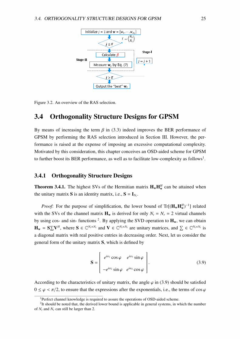
In this section, this chapter presents the simulation results along with the proposed OSD-aided scheme for characterizing the BER performance of GPSM systems, employing var-ious modulation order configurations, i.e., 4-QAM (M = 4) and 32-QAM (M = 32) asthe signal constellation. For comparison, this chapter also considers the BERs of optimalexhaustive search, i.e., the RAS scheme, and fast RAS scheme [26]. Note that TABLE3.2 lists the simulation parameter setup.
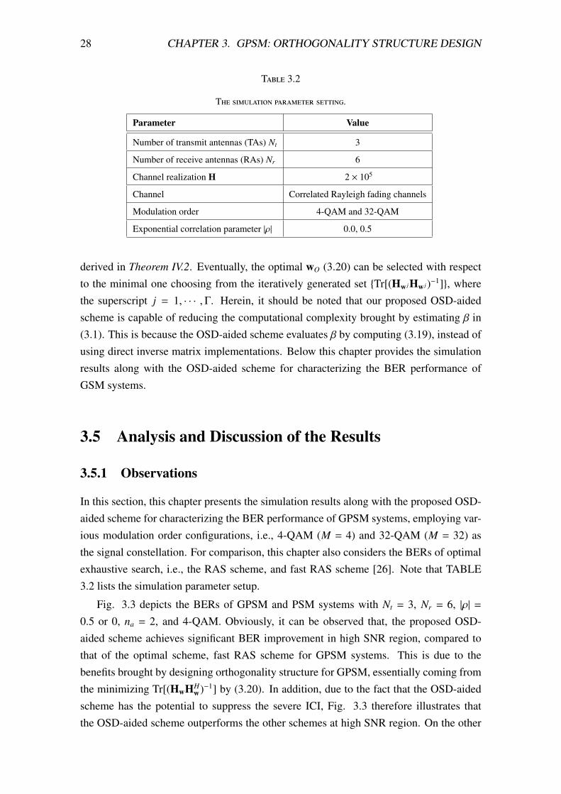
Fig. 3.3 depicts the BERs of GPSM and PSM systems with Nt = 3, Nr = 6, |ρ| =0.5 or 0, na = 2, and 4-QAM. Obviously, it can be observed that, the proposed OSD-aided scheme achieves significant BER improvement in high SNR region, compared tothat of the optimal scheme, fast RAS scheme for GPSM systems. This is due to thebenefits brought by designing orthogonality structure for GPSM, essentially coming fromthe minimizing Tr[(HwHH
w)−1] by (3.20). In addition, due to the fact that the OSD-aidedscheme has the potential to suppress the severe ICI, Fig. 3.3 therefore illustrates thatthe OSD-aided scheme outperforms the other schemes at high SNR region. On the other

3.5. ANALYSIS AND DISCUSSION OF THE RESULTS 29
0 2 4 6 8 10 12 1410
−6
10−5
10−4
10−3
10−2
10−1
100
Eb/No (dB)
BE
R
4−QAM
PSM, |ρ| = 0.5PSM, ρ = 0GPSM, Fast RAS, |ρ| = 0.5GPSM, Fast RAS, ρ = 0GPSM, OSD−aided scheme, |ρ| = 0.5GPSM, Optimal, |ρ| = 0.5GPSM, Optimal, ρ = 0 GPSM, OSD−aided scheme, ρ = 0
Figure 3.3. The BERs of fast RAS, OSD-aided scheme, and optimal scheme for GPSM and PSMsystems with Nt = 3, Nr = 6, exponential correlation parameter |ρ| = 0.5 or 0, na = 2, and 4-QAM.
0 5 10 15 20 2510
−7
10−6
10−5
10−4
10−3
10−2
10−1
100
Eb/No (dB)
BE
R
32−QAM
PSM, |ρ| = 0.5
PSM, ρ = 0
GPSM, Fast RAS, |ρ| = 0.5
GPSM, OSD−aided scheme, ρ = 0
GPSM, Fast RAS, ρ = 0
GPSM, Optimal, |ρ| = 0.5
GPSM, Optimal, ρ = 0
GPSM, OSD−aided scheme, |ρ| = 0.5
Figure 3.4. The BERs of fast RAS, OSD-aided scheme, and optimal scheme for GPSM and PSMwith Nt = 3, Nr = 6, exponential correlation parameter |ρ| = 0.5 or 0, na = 2, and 32-QAM.

30 CHAPTER 3. GPSM: ORTHOGONALITY STRUCTURE DESIGN
hand, the OSD-aided scheme curves of both ρ = 0 and |ρ| = 0.5 exhibit much better BERthan the conventional PSM.
Fig. 3.4 portrays the BERs of GPSM and PSM systems with Nt = 3, Nr = 6, |ρ|= 0.5 or 0, na = 2, and 32-QAM. Fig. 3.4 clearly shows that the OSD-aided schemeperforms good BER performance in high SNR region, compared to that of the optimalscheme, fast RAS scheme for GPSM systems. This means that the OSD-aided schemeposses both of an inherent robustness to ICI effect, and an extraordinary ability in terms ofimproving system performance, even in high-complex demodulation scenario. This is dueto the benefits brought by OSD-aided scheme, essentially coming from the minimizingTr[(HwHH
w)−1] by (3.20).By following Figs. 3.3 and 3.4, it is easy to find that the proposed OSD-aided scheme
provides 1.6 dB performance gain over the receive antenna subset selection scheme, whenBER is given at 10−5 and the modulation order is 4-QAM. On the other hand, when BER isgiven at 10−5 and the modulation order is 32-QAM, it is easy to observe that the proposedOSD-aided scheme provides 2.1 dB performance gain over the receive antenna subsetselection scheme.
3.6 Conclusion of This Chapter
In this chapter, an OSD-aided scheme was proposed to improve the performance of GPSMsystems under correlated fading channels. This chapter shows that the proposed schemescan achieve good BER performance compared to current simplified schemes. Especially,the proposed OSD-aided scheme is capable of providing significant BER performanceimprovement for GPSM systems, as well as facilitating low-complexity.

Chapter 4
Dual-Ascent Inspired TransmitPrecoding: Design & Application
31

32CHAPTER 4. DUAL-ASCENT INSPIRED TRANSMIT PRECODING: DESIGN & APPLICATION
4.1 Introduction
Recently, the increasing demand for high-speed internet services, delivering and down-loading large files, high-quality mobile video (audio) streaming, and Internet of Things(IoT) is becoming more and more popular [19]. In this sense, with the exponential growthof mobile devices and the evolution of escalating demands, it has become obligatory to in-troduce new and emerging wireless communication techniques with the prominent meritsof high data rate, energy-efficiency, spectral-efficiency, and low latency in 5G and beyondnetworks [6–10].
It is noteworthy that spatial modulation (SM) has emerged as one prospective digitalmodulation technology to improve energy-efficiency and spectral-efficiency yet maintaina low-complexity feature. In particular, the SM technique activates only a single transmitantenna (TA) out of several in each channel use, where the choice of the active anten-na is made in dependence on the data bits to be transmitted. Since SM system activatesonly a single TA in each channel use, the special structure of SM is capable of elim-inating the interchannel interference (ICI) completely at the receiver, thereby allowinglow-complexity single-stream maximum likelihood (ML) detection. To further improvethe spectral-efficiency, several variations of generalized spatial modulation (GSM) havebeen proposed by activating a portion of TAs to convey information simultaneously.
This chapter mainly focuses on the dual-ascent inspired transmit precoding designsand applications for multiple-access spatial modulation (MASM)-type MIMO systems.Notably, similar work on the transmit precoding designs and applications for MASM-MIMO has not been given yet, to the best of our knowledge. The main contributionspresent in this chapter are as follows:
• A novel MASM-MIMO system is proposed for the scenario of uplink multiple-access communications. To facilitate the system performance improvement forMASM-MIMO, this chapter focuses on the transmit precoding designs based onthe maximal-minimum Euclidean distance criterion.
• To provide a global optimum TPC solution, this chapter first recasts the above chal-lenging non-convex problems as an unconstrained problem by imposing a penaltyover the quadratic constraints.
• This chapter develops distributed approximation algorithms which have the poten-tial to refine the solution of the unconstrained problem at each iteration.
The remainder of this chapter is structured as follows: In Section 4.2 this chapterpresents the motivations for this work. In section 4.3, this chapter introduces the maximal-minimum Euclidean distance optimization problem and its solutions. In Section 4.5 thischapter describes in details the proposed BFGS-DA algorithm. In Section 4.6 this chap-ter details the experiments and the results obtained. Section 4.7 concludes this chapter

4.2. MOTIVATIONS 33
Table 4.1
List of Commonly Used Functions and Notations.
Notation Definition/Explanation
(·)T The transpose operation for the enclosed matrix/vector
(·)H The Hermitian operation for the enclosed matrix/vector
(·)−1 The inverse operation for the enclosed matrix
E [·] The statistical expectation operation
‖a‖ The l2-norm of a vector a
(a)+ The max(0, a) operation
b·c The flooring operation
⊗ The Kronecker product
� The Hadamard product
diag(x1, · · · , xN) A diagonal matrix with x1, · · · , xN as terms along its diagonal
Re {a}/Im {a} Real/Imaginary part of a complex element a
Im The identity matrix of order m
F (·) The linear search function
H (·) The real quadratic function
L (·) The Lagrange dual function
∇L (·) The gradient of the Lagrange dual function L (·)
and proposes possible directions for future work. Note that TABLE 4.1 lists the mainfunctions and notations used in this chapter.
4.2 Motivations
4.2.1 Spatial Modulation
To achieve the beamforming gain while retaining the simple design benefits of SM, avirtual SM (VSM) using multi-mode hybrid precoder has been proposed in [76]. No-tably, such VSM technology as well as its variant in [77] hold the potential to enhance thereceived signal-to-noise power ratio (SNR) and the spatial degree of freedom utilizationwith reduced radio frequency (RF) chains. By applying the concept of SM into millimeter-wave multiple-input multiple-output (MIMO), a generalized beamspace modulation usingmultiplexing (GBMM) has been developed in [78], which is a promising candidate for in-creasing the spectral-efficiency while maintaining a low-complexity transceiver structure.A comprehensive review of diverse index modulation (IM) architectures that operate inthe space, time, and frequency domains, as well as their related technologies has beenreported in [79].

34CHAPTER 4. DUAL-ASCENT INSPIRED TRANSMIT PRECODING: DESIGN & APPLICATION
4.2.2 Related Work
Various transmit precoding (TPC) techniques conceived for handling the maximal-minimumEuclidean distance (MMD) problem, or the non-convex quadratically constrained quadrat-ic program (QCQP) problem have been developed in [67] [68, 69, 75]. In particular,in [67], the MMD problem was simplified by carrying out a search only for two spe-cific parameters, i.e., the power moduli ps and pt where ps and pt represent the real partsof the TPC matrix with s , t, which might be too simple to address this non-convexproblem. In [75], the authors proposed a low-complexity iterative TPC algorithm for SM,while the BER performance of the iterative TPC algorithm degrades severely as increas-ing the number of TAs. In [68], a diagonal TPC solution was derived to address thischallenging MMD problem, however it is applicable only for two TAs. Besides, in [69],the authors converted the original non-convex MMD problem into an alternative convexproblem, followed by proposing an algorithm which iteratively approximates the optimalsolution of the convex problem. However, the performance gain is achieved at the expenseof imposing an excessive computational complexity. Based on the above observations, Ideduce that the investigation on precoder designs for SM or GSM is far from complete,and deserves a further research attention.
4.2.3 Our Idea
Against this background, this chapter focuses primally on the dual-ascent inspired TPCdesigns for multiple-access spatial modulation (MASM)-type MIMO systems. To the bestof our knowledge, similar work on the TPC designs and applications for MASM-MIMOhas not been given yet. More explicitly, to solve the challenging MMD and QCQP prob-lems, this chapter first studies the peculiarity of the convex optimization methods [80]that take the dual-ascent method into account. This beneficially provides us an insightinto developing a Broyden-Fletcher-Goldfarb-Shanno (BFGS) aided dual-ascent (BFGS-DA) algorithm that is capable of optimizing the precoding weights for all users. Next, thischapter introduces an evolving MASM-MIMO by imposing non-stationary time-varyingTPC parameters, and thereby resulting in dual-ascent aided non-stationary TPC algorith-m.
4.3 System Model
Consider the uplink of a multiple-access communication system comprised of a single BSequipped with Nr receive antennas (RAs) and K users. Each of the K users consists ofNtk (1 ≤ k ≤ K) TAs. For every time slot, there are blocks of (blog2
∏Kk=1 Ntkc + Klog2M)
bits which are arranged into the source binary streams, where M signifies the modulationorder. More explicitly, the modulation process is detailed as below. Firstly, blog2
∏Kk=1 Ntkc

4.3. SYSTEM MODEL 35
bits are fed to the SM-MIMO modulator to determine a unique TA index q for activation,which is mapped to an Ntk dimensional standard basis vector ek
q ∈ E (1 ≤ q ≤ Ntk). Next,Klog2M bits are mapped to a Gray-coded amplitude and phase modulation (APM) symbolsk
m ∈ S (m ∈ {1, · · · ,M}), where the average energy is normalized to a unit power, i.e.,E[|sm|
2] = 1. Thereby, the transmitted signal vector xk ∈ CNtk stemmed from the kth user
can be formulated as
xk = skmek
q = [0, · · · , skm, · · · , 0]T , k = 1, · · · ,K.
↑
qth
(4.1)
Next, let e = [(e1q)T , · · · , (eK
q )T ]T ∈ E be the collection of row vectors (e1q)T , · · · , (eK
q )T
from the K users, s = [s1m, · · · , s
Km]T ∈ S be the APM constellation symbol vector, and
Nt =∑K
k=1 Ntk be the summation of total TA indices of K users. Hence, the K users’ signalvector x ∈ CNt can be formulated as
x = [xT1, · · · , xT
K]T = [s1
m⊗ 11×Nt1
, · · · , sKm⊗ 11×NtK
]T � e
= [s1m, · · · , s1
m,︸ ︷︷ ︸
Nt1 terms
· · · , sKm, · · · , sK
m︸ ︷︷ ︸NtK terms
]T � [(e1q)T , · · · , (eK
q)T︸ ︷︷ ︸
Nt1 + ···+NtK terms
]T
= [s1m(e1
q)T , · · · , sK
m(eK
q)T ]T ,
(4.2)
where each symbol skm repeats Ntk times at the second step of (4.2). In particular, I observe
that x ∈ X = {S � E}, which forms the possible signal- and spatial-constellation space.
After linear diagonal precoder, x is transmitted over a wireless flat-fading MIMOchannel, and affected by an additive white Gaussian noise (AWGN). Therefore, the re-ceived signal y ∈ CNr observed at the BS can be formulated as 1
y =√ρ∑K
k=1HkUkxk + w, (4.3)
where ρ denotes the average SNR at each RA, and Hk ∈ CNr×Ntk is the channel matrix
between the kth user and the BS. w ∈ CNr is the AWGN vector with the covariance matrixσ2
wINr , and σ2w is the variance of w. Besides, Uk = diag(uk) is the diagonal TPC matrix
with the precoding weights uk = [uk,1 , · · · , uk,q , · · · , uk,Ntk]T ∈ CNtk , which is limited by
‖uk‖2≤ Ntk to enforce a transmit power normalization. Herein, uk,q is a complex-valued
precoding weight of the qth TA among user k.
1Note that, this chapter does not consider two important challenges imposed on an SM transceiver [79],i.e., the bandwidth-inefficient (time-orthogonal) shaping filter and single carrier transmissions. Such twochallenges will be discussed and analyzed in our future research.

36CHAPTER 4. DUAL-ASCENT INSPIRED TRANSMIT PRECODING: DESIGN & APPLICATION
To identify the specific influence brought by the precoding weight uk,q for the proposedMASM-MIMO, Uk ∈ C
Ntk×Ntk in (4.3) can be further decomposed as below
Uk = PkΘk = diag(pk,1e
jθk,1 , · · · , pk,qejθk,q , · · · , pk,Ntk
e jθk,Ntk
), (4.4)
where Pk = diag(pk) with pk = [pk,1 , · · · , pk,Ntk]T , and Θk = diag(θk) with θk = [θk,1, · · · , θk,Ntk
]T
are the real and imaginary parts of Uk, respectively. Besides, the introduced pk,q and θk,q
are also referred to as the power modulus and the phase angle of uk,q , respectively.
It should be noted that, when Nt1 = · · · = NtK ,∑K
k=1 Ntk = KNtk can be attained.Implicitly, this means that the proposed MASM-MIMO degenerates into the multi-userSM-MIMO with fixed TA configuration [95] [96]. In this sense, the users transmit distinctsignal blocks whose lengths are always the same at every time slot. In addition, the systemtransmission rate of (blog2
∏Kk=1 Ntkc + Klog2M) bits per channel use, i.e., the achievable
spectral-efficiency of MASM-MIMO, might be limited due to this TA constraint.
4.3.1 Maximum-Likelihood Detection
By assuming perfect channel state information (CSI) at both transmitter- and receiver-sides [97] [98], therefore, it is available for receivers (at the BS) to acquire the equiva-lent channel matrix as H = [H1, · · · ,HK] ∈ CNr×Nt . Define U = diag(u) and u =
[uT1, · · · ,uT
K]T ∈ CNt . Based on (4.3) and (4.4), the ML detector finds the estimate of s
and e jointly by solving the optimization problem of
(s, e) = arg minx∈X
‖y −√ρHUx‖2
= arg mins∈S, e∈E
‖y −√ρ∑K
k=1HkUkxk‖
2
= arg minm∈{1,··· ,M},q∈{1,··· ,Ntk }
‖y −√ρ∑K
k=1hk,quk,qsk
m‖2.
(4.5)
Accordingly, the square minimum ED d2min(H) is given by d2
min(H) = mini, j‖HUxi −HUx j‖
2.
It is straightforward that minimizing the BER performance of MASM-MIMO correspondsto maximizing the minimum ED dmin of the SM-MIMO signal points at the receiver-side via adapting those precoding weights in TPC matrix U under the power constraint∑K
k=1 ‖uk‖2≤
∑Kk=1 Ntk = Nt. Eventually, the max-d2
min based TPC matrix design can beformulated as
Uopt = arg maxU
d2min(H). (4.6)
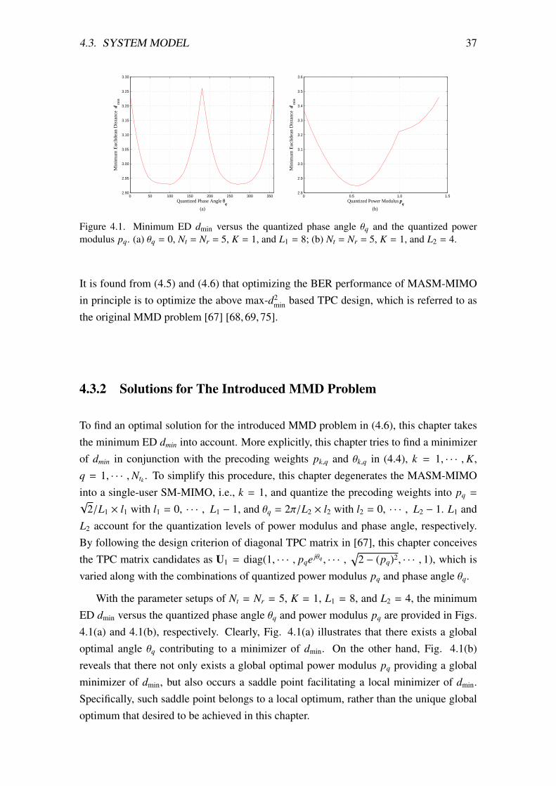
4.3. SYSTEM MODEL 37
0 50 100 150 200 250 300 3502.90
2.95
3.00
3.05
3.10
3.15
3.20
3.25
3.30
Quantized Phase Angle θq
(a)
Min
imum
Euc
lide
an D
ista
nce
d m
in
0 0.5 1.0 1.52.8
2.9
3.0
3.1
3.2
3.3
3.4
3.5
3.6
Quantized Power Modulus pq
(b)
Min
imum
Euc
lide
an D
ista
nce
d m
in
Figure 4.1. Minimum ED dmin versus the quantized phase angle θq and the quantized powermodulus pq. (a) θq = 0, Nt = Nr = 5, K = 1, and L1 = 8; (b) Nt = Nr = 5, K = 1, and L2 = 4.
It is found from (4.5) and (4.6) that optimizing the BER performance of MASM-MIMOin principle is to optimize the above max-d2
min based TPC design, which is referred to asthe original MMD problem [67] [68, 69, 75].
4.3.2 Solutions for The Introduced MMD Problem
To find an optimal solution for the introduced MMD problem in (4.6), this chapter takesthe minimum ED dmin into account. More explicitly, this chapter tries to find a minimizerof dmin in conjunction with the precoding weights pk,q and θk,q in (4.4), k = 1, · · · ,K,q = 1, · · · ,Ntk . To simplify this procedure, this chapter degenerates the MASM-MIMOinto a single-user SM-MIMO, i.e., k = 1, and quantize the precoding weights into pq =√
2/L1 × l1 with l1 = 0, · · · , L1 − 1, and θq = 2π/L2 × l2 with l2 = 0, · · · , L2 − 1. L1 andL2 account for the quantization levels of power modulus and phase angle, respectively.By following the design criterion of diagonal TPC matrix in [67], this chapter conceivesthe TPC matrix candidates as U1 = diag(1, · · · , pqe jθq , · · · ,
√2 − (pq)2, · · · , 1), which is
varied along with the combinations of quantized power modulus pq and phase angle θq.
With the parameter setups of Nt = Nr = 5, K = 1, L1 = 8, and L2 = 4, the minimumED dmin versus the quantized phase angle θq and power modulus pq are provided in Figs.4.1(a) and 4.1(b), respectively. Clearly, Fig. 4.1(a) illustrates that there exists a globaloptimal angle θq contributing to a minimizer of dmin. On the other hand, Fig. 4.1(b)reveals that there not only exists a global optimal power modulus pq providing a globalminimizer of dmin, but also occurs a saddle point facilitating a local minimizer of dmin.Specifically, such saddle point belongs to a local optimum, rather than the unique globaloptimum that desired to be achieved in this chapter.

38CHAPTER 4. DUAL-ASCENT INSPIRED TRANSMIT PRECODING: DESIGN & APPLICATION
Algorithm 1 Conventional Iteration Approach [69] for Problem (10)Input: Initialize the point u0 ← 1Nt×1; the initial iteration counter l ← 0; the predefined
threshold ε ← 10−3.Output: The final optimal point ul+1.
1: Set ul = u0.2: Solve the approximated MMD problem by updating the precoding weight vector as
belowul+1 = F (ul) .
3: Set l← l + 1.4: Until fulfill the convergence criterion ‖ul+1 − ul‖
2≤ ε.
4.3.3 Discussion
It should be noted that an efficient solution for the max-dmin based precoder design in(4.6) remains an open challenge for two reasons. Firstly, the solution depends not onlyon the dimension of H in (4.5), but also on the signal- and spatial-constellation of x in(4.2), and thus the space of solutions is vast. Secondly, finding a global optimum againstthe minimum ED dmin is indeed hard to realize. The main reason is due to the non-convexpeculiarity of MMD problem. Specifically, it is cause of that there exists at least onesaddle point influencing on the optimization in terms of maximizing the dmin. Notably,several strategies concentrating on maximizing the dmin were proposed in [99] and [100].More explicitly, [99] proposed a power allocation (PA)-aided SM under the assumptionof Θ = INt , and [100] developed a phase rotation precoding (PRP)-aided SM by lettingP = INt . Actually, such PA- or PRP-aided SM strategies with a specific TPC design mayattain only a local optimum which is caused by the saddle points. However, earlier workshave omitted this peculiarity.
4.4 Problem Statement
4.4.1 Discussion
It should be noted that, the complexity order required for solving the maximal-minimalEuclidean distance (MMD) problem employing the above CI algorithm is O
(KCIN2
t Nr
)+
O(KCIM2N4
t
), where KCI indicates the total iteration number required for addressing M-
MD problem. For easing the linear-search, the precoder design of the CI solution onlyconsiders the spatial-constellation, i.e., the optimization of the precoding weight of theCI algorithm involves an Nt-dimensional precoding vector u and an Nt × Nt-dimensionalpositive semidefinite matrix Ri, j. In contrast, the precoder optimization in [69] considersboth signal- and spatial-constellations, i.e., [69] involves an MNt-dimensional u and anMNt × MNt-dimensional Ri, j, and thereby incurring an O
(KCIM2N2
t Nr
)+ O
(KCIM4N4
t
)computational complexity.
4.5. PROPOSED APPROACH 39
4.4.2 Problem Transformation
On closer inspection, it is easy to observe that the classical MMD optimization problemis equivalent to the following optimization problem:
minu
‖u‖2
s.t. uHRi, ju ≥ Di, j, ∀ i , j,(4.7)
where Di, j is the lower bound of the ED associated with codeword pairs, and u = [uT1, · · · ,uT
K]T
∈ CNt . The design rationale behind (4.7) is to guarantee the minimum ED among the code-words, while maintaining the minimum power usage as the objective. By inspection, itis easy to find that the optimization problem in (4.7) is a large-scale non-convex QCQPproblem in that such problem imposes huge amounts of quadratic constraints with totalnumbers of NtM(NtM − 1)/2. This implies that the QCQP problem in (4.7) is intractableand solving this problem (or its relaxed problem) using the existing methods [80] willincur prohibitively high computational complexity particularly for large Nt and M.
4.5 Proposed Approach
4.5.1 The BFGS-Aided Dual-Ascent Approach
To realize the above objectives, this chapter commences by transforming the QCQPproblem in (4.7) into a real-valued form, and thereby resulting in a real vector m =
[mT1 · · ·m
TK]T = [pT θT ]T , where mk (1 ≤ k ≤ K) corresponds to the real weighting
vector for user k. Herein, p = [pT1 · · · p
TK]T and θ = [θT
1 · · ·θTK]T . Next, this chapter
converts the positive semidefinite matrix Ri, j in (4.7) into a real matrix [101]
Gi, j =
Re{Ri, j} −Im{Ri, j}
Im{Ri, j} Re{Ri, j}
. (4.8)
Hereinafter,H({m1, · · · ,mK}, Gi, j
)= [mT
1 · · ·mTK] Gi, j [mT
1 · · ·mTK]T is used to denote the
real quadratic function, which is positive definite for any real weighting vector [mT1 · · ·m
TK]T .
Following the QCQP problem in (4.7), it is easy to observe that the solution to theproblem in (4.7) can guarantee the minimum ED among the codewords while maintainingthe minimum power usage. However, when taking the MASM-MIMO into account, it isneeded to find a new solution to approach the minimum ED, at the same time to ensureminimum power usage for each single user. To cope with this quadratic-programmingtype optimization, this chapter therefore designs the below optimization problem (P2).Note that, the proposed design in (4.9) requires full channel information of all users.

40CHAPTER 4. DUAL-ASCENT INSPIRED TRANSMIT PRECODING: DESIGN & APPLICATION
This chapter assumes that the channel statistics are perfectly known and shared amongusers [97] [98], such that full channel information can be estimated accordingly. Notealso that, the estimation of full channel information requires a significant overhead forrealizing it, which continues to be a challenge.
minm1, ··· ,mK
∑K
k=1mT
k mk
s.t. H({m1, · · · ,mK}, Gi, j
)≥ Di, j, ∀ i , j.
(4.9)
Subsequently, to approximately formulate the inequality constrained problem in P2 asan equality constrained problem, this chapter next formulates a Lagrange dual function asbelow
L ({m1, · · · ,mK}, s, y, µ) =
K∑k=1
mTk mk
−
Nt∑i=1
Nt∑j=1, j,i
yi, j
(H
({m1, · · · ,mK},Gi, j
)− si, j − Di, j
)+
Nt∑i=1
Nt∑j=1, j,i
µ(H
({m1, · · · ,mK},Gi, j
)− si, j − Di, j
)2,
(4.10)
where the introduced y = {yi, j} is a Lagrange multiplier inspired dual vector, s = {si, j} is aslack vector satisfying thatH
({m1, · · · ,mK},Gi, j
)= si, j + Di, j and si, j > 0. µ > 0 denotes
the penalty weight, and the quadratic approximation∑Nt
i=1
∑Ntj=1, j,i(H
({m1, · · · ,mK},Gi, j
)−
si, j − Di, j)2 is the penalty item. Note that the value of Nt = MNt influences the numberof the quadratic constraints in P2. Furthermore, the value of Nt indicates the dimensionof the involved Lagrange dual function variables (i.e., the positive semidefinite matrixGi, j, the dual vector y, the slack vector s, and Di, j), and thus can implicitly determine thesolution space of L ({m1, · · · ,mK}, s, y, µ) in (4.10).
Following the updating criterion of primal vectors in the dual-ascent method [80],this chapter next minimizes the Lagrange dual function L ({m1, · · · ,mK}, s, y, µ) in (4.10)with respect to (w.r.t.) m1, · · · ,mK , and s at the kth iteration as follow
minm1, ··· ,mK , s
L ({m1, · · · ,mK}, s, yk, µk)
s.t. s ≥ 0.(4.11)
Subsequently, this chapter calculates the gradient function of L ({m1, · · · ,mK}, s, yk, µk)
w.r.t. the slack variable si, j, which is denoted by ∇sL ({m1, · · · ,mK}, s, yk, µk). To get ridof the influence brought by the slack variables, this chapter minimizesL ({m1, · · · ,mK}, s, yk, µk)
4.5. PROPOSED APPROACH 41
in (4.11) w.r.t. each of the si, j separately. With ∇sL ({m1, · · · ,mK}, s, yk, µk) = 0, it there-fore can attain that
si, j = H({m1, · · · ,mK},Gi, j
)− Di, j −
yi, j,k
2µk. (4.12)
If this unconstrained minimizer is smaller than the lower bound of 0, then since (4.11) isconvex in si, j, the optimal value of si, j will be 0. Hence, the optimal value of si, j is givenby si, j =
(H
({m1, · · · ,mK},Gi, j
)− Di, j −
yi, j,k
2µk
)+. Submitting this optimal value of si, j
back into (4.10) results in a new Lagrange dual function L ({m1, · · · ,mK}, yk, µk), whichis given by (4.13) shown at the top of next page.
L ({m1, · · · ,mK}, yk, µk) =
K∑γ=1
mTγmγ −
Nt∑i=1
Nt∑j=1, j,i
yi, j,k(H
({m1, · · · ,mK},Gi, j
)− Di, j
)+
Nt∑i=1
Nt∑j=1, j,i
µk(H
({m1, · · · ,mK},Gi, j
)− Di, j
)2,H
({m1, · · · ,mK},Gi, j
)− Di, j ≤
yi, j,k
2µk,
K∑γ=1
mTγmγ −
Nt∑i=1
Nt∑j=1, j,i
y2i, j,k
4µk, H
({m1, · · · ,mK},Gi, j
)− Di, j >
yi, j,k
2µk,
(4.13)
Notably, my optimization objective then turns into approximating the minimizer ofL({m1, · · · ,mK}, yk, µk) in (4.13), which is referred to as the unconstrained minimization
problem. By exploiting the dual-ascent framework [80] and leveraging the BFGS algorith-m [101] [102], this chapter next approximates the minimizer of L({m1, · · · ,mK}, yk, µk),so as to tackle this unconstrained minimization problem and find the primal optimal vec-tors of m1, · · · ,mK . To carry out the BFGS algorithm, this chapter next needs to calculatethe gradient function ofL({m1, · · · ,mK}, yk, µk), which is provided by the following Lem-ma IV.1.

42CHAPTER 4. DUAL-ASCENT INSPIRED TRANSMIT PRECODING: DESIGN & APPLICATION
Lemma 4.5.1. In general, the gradient function of L ({m1, · · · ,mK}, yk, µk) w.r.t. the pri-mal vector mγ, 1 ≤ γ ≤ K, is given by
∇mγL ({m1, · · · ,mK}, yk, µk) =
2mγ +
Nt∑i=1
Nt∑j=1, j,i
(4µk
(H({m1, · · · ,mK},Gi, j) − Di, j
)− 2yi, j,k
)
×
(G(i)γ,( j)γmγ +
K∑j′=1, j′,γ
G(i)γ,( j) j′m j′
), H
({m1, · · · ,mK},Gi, j
)− Di, j ≤
yi, j,k
2µk,
2mγ, H({m1, · · · ,mK},Gi, j
)− Di, j >
yi, j,k
2µk.
(4.14)
Proof of Lemma IV.1: By following (4.13) and under the constraint ofH({m1, · · · ,mK},Gi, j)−Di, j ≤
yi, j,k
2µk, it is easy to obtain the associated Lagrange dual functionL ({m1, · · · ,mK}, yk, µk)
at the kth iteration given by
L ({m1, · · · ,mK}, yk, µk) =
K∑γ=1
mTγmγ
−
Nt∑i=1
Nt∑j=1, j,i
yi, j,k(H
({m1, · · · ,mK},Gi, j
)− Di, j
)+
Nt∑i=1
Nt∑j=1, j,i
µk(H
({m1, · · · ,mK},Gi, j
)− Di, j
)2.
(4.15)
For H({m1, · · · ,mK},Gi, j
)− Di, j >
yi, j,k
2µk, the above mentioned Lagrange dual function
L ({m1, · · · ,mK}, yk, µk) at the kth iteration is given by
L({m1, · · · ,mK}, yk, µk) =
K∑γ=1
mTγmγ −
Nt∑i=1
Nt∑j=1, j,i
y2i, j,k
4µk. (4.16)
This chapter next calculates the gradient of L ({m1, · · · ,mK}, yk, µk) in (4.15) and (4.16)w.r.t. the primal vector mγ, 1 ≤ γ ≤ K, respectively. Observing that both primal and dualvariables are defined in real-valued form, this chapter thereby can easily derive the gradi-ent of the Lagrange dual functionL({m1, · · · ,mK}, yk, µk) in (4.16) as∇mγ
L({m1, · · · ,mK}, yk, µk) =
2mγ.
Observing that (4.15) contains a positive definiteH({m1, · · · ,mK},Gi, j
)in its last two
items, it seems intractable to calculate the gradient of L({m1, · · · ,mK}, yk, µk) w.r.t. mγ
directly. In contrast, this chapter substitutes (4.8) into H({m1, · · · ,mK},Gi, j
), and then
4.5. PROPOSED APPROACH 43
can arrive at that
H({m1, · · · ,mK},Gi, j) = [mT1 · · ·m
TK] Gi, j [mT
1 · · ·mTK]T
=
K∑γ=1
mTγG(i)γ,( j)γmγ +
K∑i′=1
K∑j′=1, j′,i′
mTi′G(i)i′ ,( j) j′m j′ ,
(4.17)
where G(i)i′ ,( j) j′ denotes the submatrix of Gi, j and inherits the properties of Ri, j. For in-stance, G(i)γ,( j)γ is given by
G(i)γ,( j)γ =
Re{(Ri, j)γ,γ} −Im{(Ri, j)γ,γ}
Im{(Ri, j)γ,γ} Re{(Ri, j)γ,γ}
, (4.18)
where (Ri, j)γ,γ = HHγ Hγ � ∆XT
i, j and ∆Xi, j = ((xγ)i − (xγ) j)((xγ)i − (xγ) j)H. By substituting(4.17) back into (4.15) and then calculating the gradient of (4.15), it can be arrived at that
∇mγL({m1, · · · ,mK}, yk, µk) = 2mγ +
Nt∑i=1
Nt∑j=1, j,i
(4µk
×
([mT
1 · · ·mTK] Gi, j [mT
1 · · ·mTK]T − Di, j
)− 2yi, j,k
)×
(G(i)γ,( j)γmγ +
K∑j′=1, j′,γ
G(i)γ,( j) j′m j′
).
(4.19)
Combining (4.19) and ∇mγ
(∑Kγ=1 mT
γmγ
)= 2mγ together leads to Lemma IV.1. This
completes the proof of Lemma IV.1. �
4.5.2 Discussion
Theorem 4.5.2. Since [mT1 · · ·m
TK] Gi, j [mT
1 · · ·mTK]T is positive definite, this chapter de-
duces that L ({m1, · · · ,mK}, s, y, µ) > L({mk+1
1 , · · · ,mk+1K }, s, y, µ
). Thereby, this chapter
concludes that {mk+11 , · · · ,mk+1
K } is the unique global minimizer ofL ({m1, · · · ,mK}, s, y, µ)
in (4.10).
Proof of Theorem IV.2: Recall that m = [mT1 · · ·m
TK]T is a real-valued vector. By
using our proposed BFGS-DA algorithm, it can attain mk+1 = [(mk+11 )T · · · (mk+1
K )T ]T
serving as the optimal primal vector. Hereinafter, this chapter use m and mk+1 to replace[mT
1 · · ·mTK]T and [(mk+1
1 )T · · · (mk+1K )T ]T , and useL (m, s, y, µ) to replaceL ({m1, · · · ,mK}, s, y, µ)
in (4.10) for ease of convenient representation.
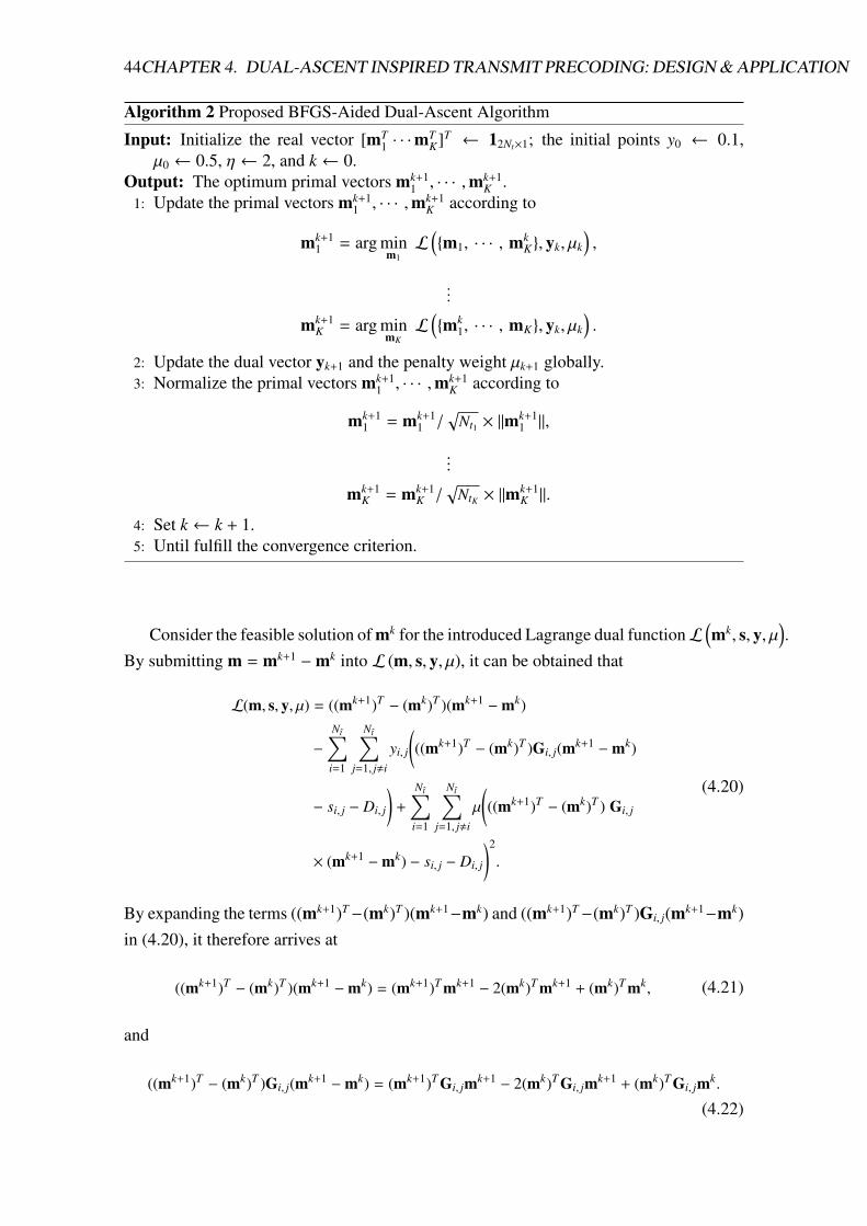
44CHAPTER 4. DUAL-ASCENT INSPIRED TRANSMIT PRECODING: DESIGN & APPLICATION
Algorithm 2 Proposed BFGS-Aided Dual-Ascent Algorithm
Input: Initialize the real vector [mT1 · · ·m
TK]T ← 12Nt×1; the initial points y0 ← 0.1,
µ0 ← 0.5, η ← 2, and k ← 0.Output: The optimum primal vectors mk+1
1 , · · · ,mk+1K .
1: Update the primal vectors mk+11 , · · · ,mk+1
K according to
mk+11 = arg min
m1L
({m1, · · · , mk
K}, yk, µk
),
...
mk+1K = arg min
mKL
({mk
1, · · · , mK}, yk, µk
).
2: Update the dual vector yk+1 and the penalty weight µk+1 globally.3: Normalize the primal vectors mk+1
1 , · · · ,mk+1K according to
mk+11 = mk+1
1 /√
Nt1 × ‖mk+11 ‖,
...
mk+1K = mk+1
K /√
NtK × ‖mk+1K ‖.
4: Set k ← k + 1.5: Until fulfill the convergence criterion.
Consider the feasible solution of mk for the introduced Lagrange dual functionL(mk, s, y, µ
).
By submitting m = mk+1 −mk into L (m, s, y, µ), it can be obtained that
L(m, s, y, µ) = ((mk+1)T − (mk)T )(mk+1 −mk)
−
Nt∑i=1
Nt∑j=1, j,i
yi, j
(((mk+1)T − (mk)T )Gi, j(mk+1 −mk)
− si, j − Di, j
)+
Nt∑i=1
Nt∑j=1, j,i
µ
(((mk+1)T − (mk)T ) Gi, j
× (mk+1 −mk) − si, j − Di, j
)2
.
(4.20)
By expanding the terms ((mk+1)T−(mk)T )(mk+1−mk) and ((mk+1)T−(mk)T )Gi, j(mk+1−mk)in (4.20), it therefore arrives at
((mk+1)T − (mk)T )(mk+1 −mk) = (mk+1)T mk+1 − 2(mk)T mk+1 + (mk)T mk, (4.21)
and
((mk+1)T − (mk)T )Gi, j(mk+1 −mk) = (mk+1)T Gi, jmk+1 − 2(mk)T Gi, jmk+1 + (mk)T Gi, jmk.
(4.22)

4.5. PROPOSED APPROACH 45
Table 4.2Complexity Comparisons Among Different Precoding Schemes
PrecodingScheme
Complexity Order
DiagonalTPC [67]
O(L1L2M2N2
t Nr
)CI [69] O
(KCI M2N2
t Nr
)+ O
(KCI M4N4
t
)BFGS-DA O
(KDAN2
t Nr
)+ O
(KDAKN2
t lBFGS
)+ O
(KDAKN2
t N2t
)
By substituting (4.21) and (4.22) back into (4.20), this chapter therefore can arrive at (43)shown at the top of next page.
In addition, the slack and penalty variables involved in (4.10) satisfy the below con-straints:
mT Gi, jm − si, j − Di, j = 0, ∀ i , j, (44a)
si, j > 0, and µ > 0, ∀ i , j, (44b)
m −Nt∑i=1
Nt∑j=1, j,i
yi, jGi, jm +
Nt∑i=1
Nt∑j=1, j,i
2µ(mT Gi, jm − si, j − Di, j
)Gi, jm = 0. (44c)
Properly, combining (44a) and (44c) together implies m =∑Nt
i=1
∑Ntj=1, j,i yi, jGi, jm. Observ-
ing (mk)T mk+1 =∑Nt
i=1
∑Ntj=1, j,i yi, j(mk)T Gi, jmk+1, (43) therefore can be rewritten by (45)
shown at the top of this page. In (45), let (a) = (mk)T mk −∑Nt
i=1
∑Ntj=1, j,i yi, j
((mk)T Gi, jmk
),
and (b) =∑Nt
i=1
∑Ntj=1, j,i µ
((mk)T Gi, jmk − 2(mk)T Gi, jmk+1
)2. Observing the result that
(mk)T mk =∑Nt
i=1
∑Ntj=1, j,i yi, j(mk)T Gi, jmk, it therefore can arrive at (a) = 0. In addition,
due to the fact that µ > 0 and (mk)T Gi, jmk+1 > (mk)T Gi, jmk, it thus can have (b) > 0.By submitting (a) = 0 and (b) > 0 back into (45), this chapter deduces L(m, s, y, µ) >L(mk+1, s, y, µ), and thereby concluding that mk+1 = [(mk+1
1 )T · · · (mk+1K )T ]T is the unique
global minimizer of L({m1, · · · ,mK}, s, y, µ). This completes the proof of Theorem IV.2.�
4.5.3 Complexity Analysis
In this subsection, this chapter estimates the computational complexity of the BFGS-DAscheme and compare the estimated complexity with that of the diagonal TPC [67] andCI [69] precoding schemes. Notably, the overall complexity of BFGS-DA is incurred bytwo major operations performed in Alg. 2, i.e., the operations required for approximating

46CHAPTER 4. DUAL-ASCENT INSPIRED TRANSMIT PRECODING: DESIGN & APPLICATION
Table 4.3Operation Number Comparisons for Different Precoding Schemes in Single-/Multi-User Scenarios
PrecodingScheme
Single-userCase
Multi-userCase
CI [69] 16793600 268500992
BFGS-DA 1058560 2101888
the global optimal primal vectors mk+11 , · · · ,mk+1
K , as well as for updating the dual vectory. For each iteration, Alg. 2 approximates the global optimal primal vectors by exploitingthe BFGS algorithm [102], and thereby incurring an O(KN2
t lBFGS ) + O(KN2t N2
t ) compu-tational complexity with Nt = MNt. On the other hand, Alg. 2 updates the dual vector yby following the criterion of (21) in [22], which accordingly imposes an O(N2
t Nr) com-plexity at each iteration. The overall complexity of BFGS-DA therefore can be countedas O(KDAKN2
t lBFGS ) + O(KDAKN2t N2
t ) + O(KDAN2t Nr) with KDA being the total iteration
number of BFGS-DA required for reaching the convergence. Accordingly, the complexitycomparisons of the above three schemes are given in TABLE II.
A further comparison of the complexity order of different precoder design for Nt = 16,K = 1, Nr = 4, 4-QAM (single-user scenario) and Nt = 8, K = 2, Nr = 4, 16-QAM (multi-user scenario) is provided in TABLE III. Note that this chapter compares the complexityorder of different precoder design at each single iteration. Note also that the number ofiterations of BFGS in TABLE III is assumed to be lBFGS = 35, given that usually BFGS issuccessful with lBFGS ∈ [2, 35] [102]. By following the results in TABLE III, it is evidentthat for solving the introduced convex problem, the BFGS-DA scheme requires a low andmanageable computational complexity relative to the CI scheme [69] for both the single-and multi-user scenarios. It should be noted that analysis of the convergence behavior ofBFGS-DA is omitted.
4.6 Experimental Results
4.6.1 BER Performance Evaluations
Note that TABLE 4.4 lists the simulation parameter setup. Fig. 4.2 exhibits the BERsof single-user SM-MIMO and MASM-MIMO with the diagonal TPC [67] 2, the CI [69],the TAC [103], and the proposed BFGS-DA schemes for the scenarios of Nt1 = 8, K =
1, Nr = 2 and 4, and M = 4. Note that the MASM-MIMO in Fig. 4.2 degenerates intothe single-user SM-MIMO case. More explicitly, it is easy to observe from Fig. 4.2 that
2Note that the quantization levels of amplitude and phase for the diagonal TPC scheme are assumed tobe L1 = 6 and L2 = 6, respectively.
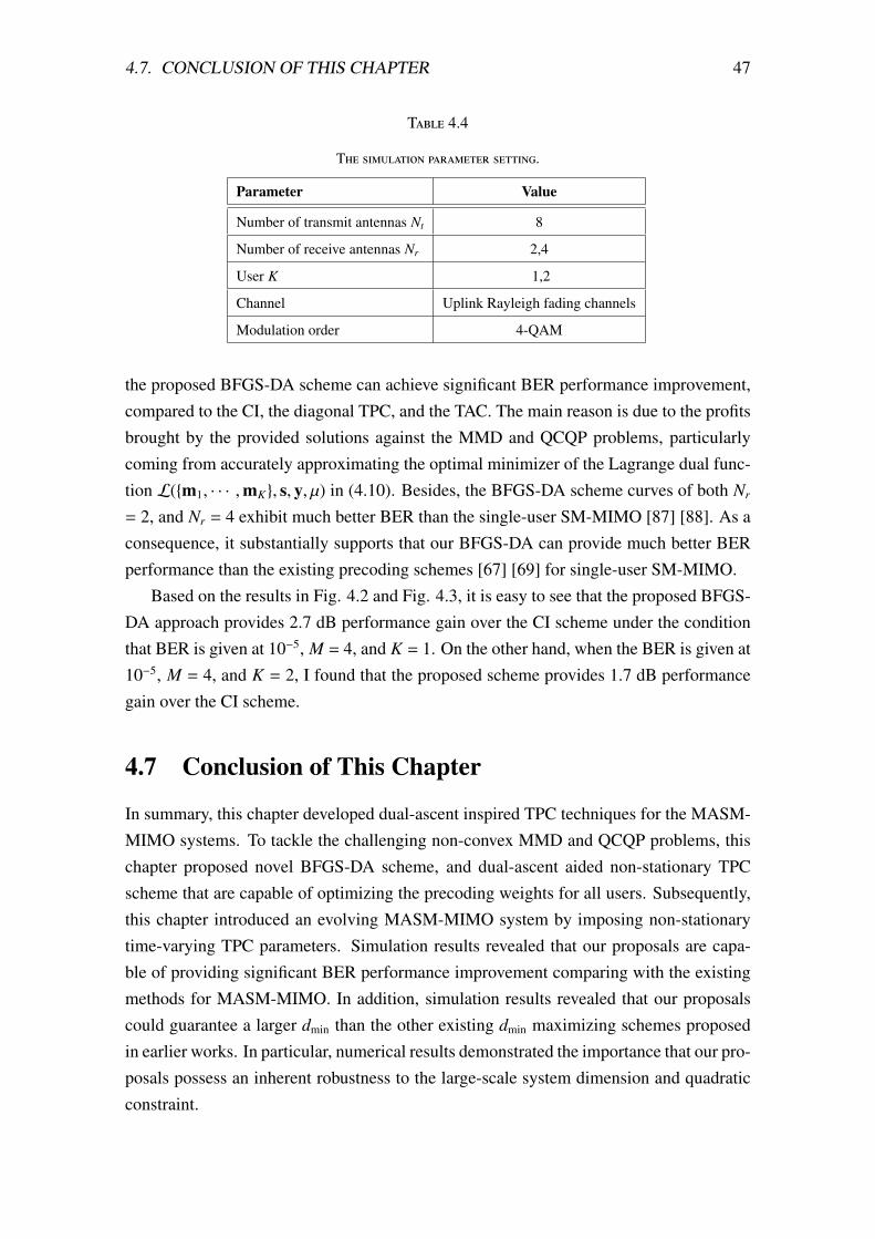
4.7. CONCLUSION OF THIS CHAPTER 47
Table 4.4
The simulation parameter setting.
Parameter Value
Number of transmit antennas Nt 8
Number of receive antennas Nr 2,4
User K 1,2
Channel Uplink Rayleigh fading channels
Modulation order 4-QAM
the proposed BFGS-DA scheme can achieve significant BER performance improvement,compared to the CI, the diagonal TPC, and the TAC. The main reason is due to the profitsbrought by the provided solutions against the MMD and QCQP problems, particularlycoming from accurately approximating the optimal minimizer of the Lagrange dual func-tion L({m1, · · · ,mK}, s, y, µ) in (4.10). Besides, the BFGS-DA scheme curves of both Nr
= 2, and Nr = 4 exhibit much better BER than the single-user SM-MIMO [87] [88]. As aconsequence, it substantially supports that our BFGS-DA can provide much better BERperformance than the existing precoding schemes [67] [69] for single-user SM-MIMO.
Based on the results in Fig. 4.2 and Fig. 4.3, it is easy to see that the proposed BFGS-DA approach provides 2.7 dB performance gain over the CI scheme under the conditionthat BER is given at 10−5, M = 4, and K = 1. On the other hand, when the BER is given at10−5, M = 4, and K = 2, I found that the proposed scheme provides 1.7 dB performancegain over the CI scheme.
4.7 Conclusion of This Chapter
In summary, this chapter developed dual-ascent inspired TPC techniques for the MASM-MIMO systems. To tackle the challenging non-convex MMD and QCQP problems, thischapter proposed novel BFGS-DA scheme, and dual-ascent aided non-stationary TPCscheme that are capable of optimizing the precoding weights for all users. Subsequently,this chapter introduced an evolving MASM-MIMO system by imposing non-stationarytime-varying TPC parameters. Simulation results revealed that our proposals are capa-ble of providing significant BER performance improvement comparing with the existingmethods for MASM-MIMO. In addition, simulation results revealed that our proposalscould guarantee a larger dmin than the other existing dmin maximizing schemes proposedin earlier works. In particular, numerical results demonstrated the importance that our pro-posals possess an inherent robustness to the large-scale system dimension and quadraticconstraint.

48CHAPTER 4. DUAL-ASCENT INSPIRED TRANSMIT PRECODING: DESIGN & APPLICATION
0 5 10 15 20
Eb/No (dB)
10-5
10-4
10-3
10-2
10-1
100
BE
R
K=1 & 4-QAMSingle-user SM-MIMOSingle-user SM-MIMO + TACSingle-user SM-MIMO + Diagonal TPCSingle-user SM-MIMO + CIMASM-MIMO + BFGS-DA
Nr = 4
Nr = 2
Figure 4.2. The BERs of the TAC, the diagonal TPC, the CI, and the proposed BFGS-DA schemesfor single-user SM-MIMO and MASM-MIMO systems with Nt1 = 8, K = 1, Nr = 2 or 4, andM = 4.
0 5 10 15 20
Eb/No (dB)
10-5
10-4
10-3
10-2
10-1
100
BE
R
K=2 & 4-QAM
Multi-user SM-MIMOMulti-user SM-MIMO + Diagonal TPCMulti-user SM-MIMO + TACGSM-MIMO with K active antennasMulti-user SM-MIMO + CIMASM-MIMO + BFGS-DA
Figure 4.3. The BERs of the diagonal TPC, the TAC, the CI, and the proposed BFGS-DA schemesfor multi-user SM-MIMO and MASM-MIMO, as well as GSM-MIMO with Nt1 = Nt2 = 8, K = 2,Nr = 4, and M = 4.

Chapter 5
Beam and Power Allocation Using DeepLearning
49
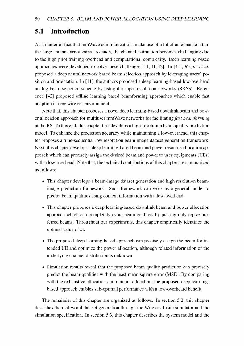
50 CHAPTER 5. BEAM AND POWER ALLOCATION USING DEEP LEARNING
5.1 Introduction
As a matter of fact that mmWave communications make use of a lot of antennas to attainthe large antenna array gains. As such, the channel estimation becomes challenging dueto the high pilot training overhead and computational complexity. Deep learning basedapproaches were developed to solve these challenges [11, 41, 42]. In [41], Rezaie et al.
proposed a deep neural network based beam selection approach by leveraging users’ po-sition and orientation. In [11], the authors proposed a deep learning-based low-overheadanalog beam selection scheme by using the super-resolution networks (SRNs). Refer-ence [42] proposed offline learning based beamforming approaches which enable fastadaption in new wireless environment.
Note that, this chapter proposes a novel deep learning-based downlink beam and pow-er allocation approach for multiuser mmWave networks for facilitating fast beamforming
at the BS. To this end, this chapter first develops a high-resolution beam quality predictionmodel. To enhance the prediction accuracy while maintaining a low-overhead, this chap-ter proposes a time-sequential low resolution beam image dataset generation framework.Next, this chapter develops a deep learning-based beam and power resource allocation ap-proach which can precisely assign the desired beam and power to user equipments (UEs)with a low-overhead. Note that, the technical contributions of this chapter are summarizedas follows:
• This chapter develops a beam-image dataset generation and high resolution beam-image prediction framework. Such framework can work as a general model topredict beam qualities using context information with a low-overhead.
• This chapter proposes a deep learning-based downlink beam and power allocationapproach which can completely avoid beam conflicts by picking only top-m pre-ferred beams. Throughout our experiments, this chapter empirically identifies theoptimal value of m.
• The proposed deep learning-based approach can precisely assign the beam for in-tended UE and optimize the power allocation, although related information of theunderlying channel distribution is unknown.
• Simulation results reveal that the proposed beam-quality prediction can preciselypredict the beam-qualities with the least mean square error (MSE). By comparingwith the exhaustive allocation and random allocation, the proposed deep learning-based approach enables sub-optimal performance with a low-overheard benefit.
The remainder of this chapter are organized as follows. In section 5.2, this chapterdescribes the real-world dataset generation through the Wireless Insite simulator and thesimulation specification. In section 5.3, this chapter describes the system model and the

5.2. DATA 51
Table 5.1
List of Commonly Used Functions and Notations.
Notation Definition/Explanation
(·)T The transpose operation for the enclosed matrix/vector
(·)H The Hermitian operation for the enclosed matrix/vector
|| · || The l2-norm operation
(·)†
The pseudo-inversion of a vector
‖a‖ The l2-norm of a vector a
⊗ The Kronecker product
channel model of this chapter. In section 5.4 this chapter states the problem formulationand the problem transformation of this chapter. In section 5.6, this chapter introduces theoptimal allocation approach and the deep learning based approach for precisely assigningthe beam for intended UE and optimizing the power allocation with low-overhead. In sec-tion 5.7 this chapter shows the simulation results of our proposal in comparison with theoptimal allocation approach and the random allocation approach. Besides, this chapteranalyzes the obtained results, followed by giving related reasons for achieving the perfor-mance benefits of our approach. Finally, section 5.8 makes a conclusion of this chapter.Note that TABLE 5.1 lists the main functions and notations used in this chapter.
5.2 Data
5.2.1 Realistic Channel Generation
Note that this chapter uses the Wireless Insite simulator [104] to generate realistic chan-nel vectors including the angle of arrival (AoA), angle of departure (AoD), path loss, etc.Moreover, the Wireless Insite is a ray-tracing simulator considering the diffraction and thepenetration of each path given communication systems and environment settings [11]. In-tuitively, the simulation environment in the wireless insite simulator is provided in Figure5.1.
5.2.2 Simulation Specification
On the other hand, this chapter describes the simulation specification including the trans-mitter set/receiver set setting as shown in Figure 5.2, the carrier frequency f setting, theeffective bandwidth B setting. In this work, this chapter sets the dimension of transmitter(the BS) to be 64, the dimension of the receiver (user equipment) to be 1, the carrier fre-quency f to be 60GHz, the effective bandwidth B to be 100MHz, the height of BS to be
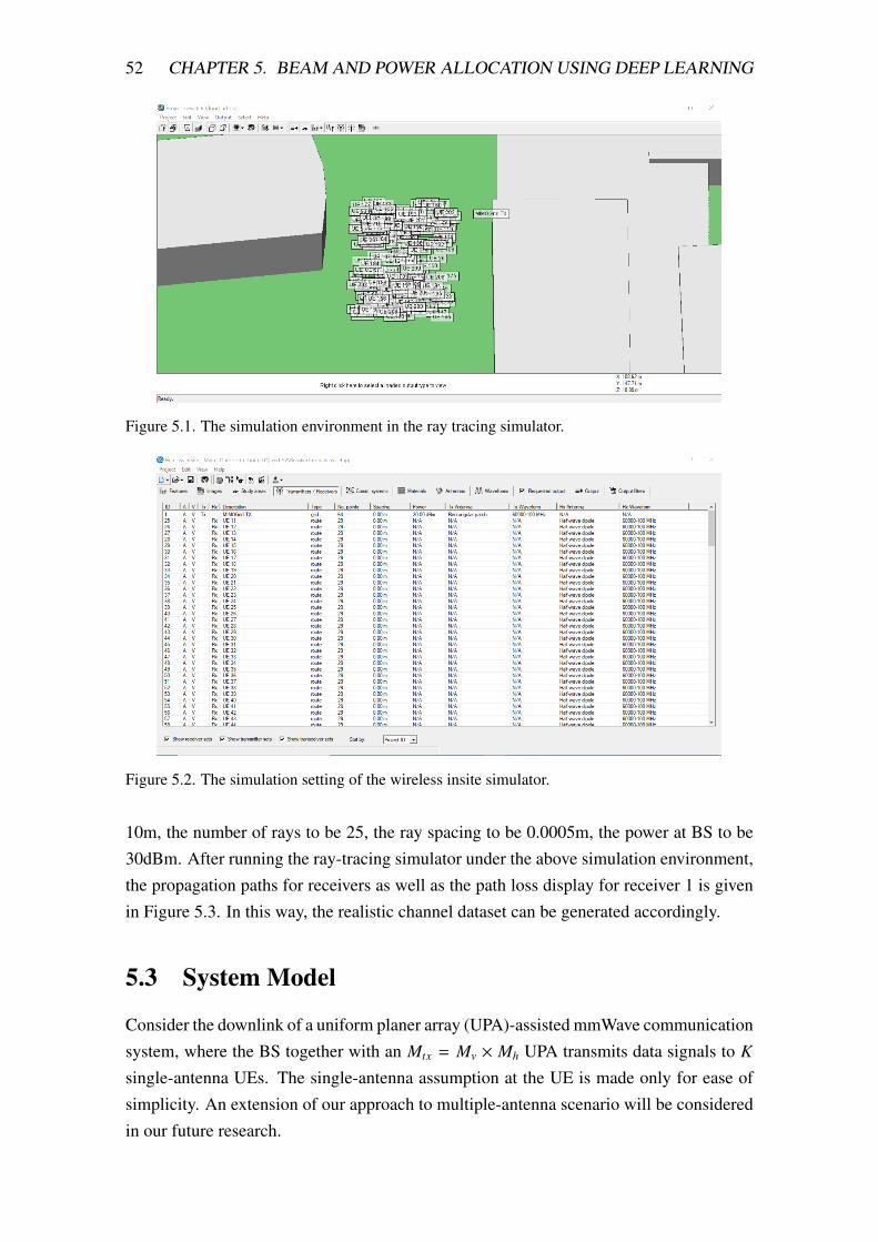
52 CHAPTER 5. BEAM AND POWER ALLOCATION USING DEEP LEARNING
Figure 5.1. The simulation environment in the ray tracing simulator.
Figure 5.2. The simulation setting of the wireless insite simulator.
10m, the number of rays to be 25, the ray spacing to be 0.0005m, the power at BS to be30dBm. After running the ray-tracing simulator under the above simulation environment,the propagation paths for receivers as well as the path loss display for receiver 1 is givenin Figure 5.3. In this way, the realistic channel dataset can be generated accordingly.
5.3 System Model
Consider the downlink of a uniform planer array (UPA)-assisted mmWave communicationsystem, where the BS together with an Mtx = Mv × Mh UPA transmits data signals to K
single-antenna UEs. The single-antenna assumption at the UE is made only for ease ofsimplicity. An extension of our approach to multiple-antenna scenario will be consideredin our future research.

5.3. SYSTEM MODEL 53
Figure 5.3. The propagation paths for receivers.
5.3.1 Channel Model
This chapter considers the mmWave channel model where the BS serves K UEs withcarrier frequency f = 60 GHz. Given that the proposed beamforming approach makesuse of the spatial correlation between the channel and the beamforming directions, it istherefore essential to generate realistic channel vectors including the AoA, AoD, pathloss, etc.
Based on geometry, the phase differences of a training signal between the antennaelements can be represented as a steering vector. In particular, the steering vector of thevertical axis and the horizontal axis are expressed as follows
av(φ) =
[1, e− j2πdv cos(φ)/λ, · · · , e− j2π(Mv−1)dv cos(φ)/λ
]T
, (5.1)
ah(ϕ,φ) =
[1, e− j2πdh sin(φ) sin(ϕ)/λ, · · · , e− j2π(Mh−1)dh sin(φ) sin(ϕ)/λ
]T
, (5.2)
where λ refers to the wavelength. dv and dh represent the distances between vertical andhorizontal antenna elements, respectively. Kronecker product makes it possible to expressthe steering vector of a UPA in the form of a(ϕ,φ) = av(φ) ⊗ ah(ϕ,φ).
5.3.2 Beamforming Weights
The beamforming weight vector associated with UE k ∈ {1, · · · ,K} after applying to aUPA can be expressed as wk,n = wv
k,n ⊗whk,n, where n ∈ {1, · · · ,N}, and N indicates the re-
quired number of broadcasting rounds.1 wvk,n = [wv
1, · · · ,wvMv
]T and whk,n = [wh
1, · · · ,whMh
]T
1Notice that, herein the required broadcasting rounds N in fact is equal to the total number of beamsMtx.

54 CHAPTER 5. BEAM AND POWER ALLOCATION USING DEEP LEARNING
are the weights on antenna elements along the vertical and horizontal directions, respec-tively. In this way, the analog beamforming weight associated with K UEs therefore canbe expressed as
Wn =[wv
1,n ⊗ wh1,n, · · · , wv
K,n ⊗ whK,n
]. (5.3)
As a merit of our approach, total number of only mtx =√
mtx ×√
mtx low-resolutionbeams is required and served as an input to our neural networks to predict the analogbeamforming for each UE, i.e., mtx ≤ Mtx, and thus can greatly reduce the training over-head. On the other hand, this chapter definesW as the standard discrete Fourier transform(DFT)-based codebook for the UPA-based transmitter. In the training phase, the UPA ap-plies the DFT codebook-based analog beamforming architecture to beamform signals.
5.3.3 Downlink Beam Broadcasting
In our considered system, the BS first sweeps the beams by broadcasting beams to UEsin sequential time slots. After applying the analog beamformer wk,n ∈ W, the receivedsignal rk at the UE k therefore can be expressed as
rk =√
pkhHk wk,ns +
∑i,k
√pihH
k wi,ns + nk, (5.4)
where hk ∈ CMtx denotes the channel coefficient between the BS and UE k. pk and s repre-
sent the transmit power budget for UE k ∈ {1, · · · ,K} and the known training signal withnormalized power, respectively. nk corresponds to additive white Gaussian noise (AWGN)with zero mean and variance N0. The noise power N0 at UEs is N0 = kBT BF with kB beingthe Boltzmann constant, T being the absolute temperature, B being the bandwidth, and F
being the noise figure. Based on the received training signals in a beam sweeping, the UEfeedbacks the measured received signals to the BS through the mmWave control channelfor performing the subsequent beam-quality prediction and channel estimation.
For ∀UE k ∈ {1, · · · ,K}, the signal-to-interference-plus-noise ratio (SINR) associatedwith the downlink allocation policy
(wk,n, pk
)is
γk(wk,n, pk) =pk‖hH
k wk,n‖2∑
i,k pi
∥∥∥hHk wi,n
∥∥∥2+ N0
. (5.5)
Notice that for the multiuser mmWave scenario, i.e., K ≥ 2, accurately estimate the beamhaving the largest received power by UEs will become difficult in the sense that UEs whoare geographically co-located together maybe wrongly allocated the same desired beam(i.e., the codeword), thus significantly deteriorating the system performance.

5.4. PROBLEM STATEMENT 55
5.4 Problem Statement
5.4.1 Sum-Rate Maximization Problem
The purpose of our approach is to predict the beam qualities for the next communicationround, followed by properly allocating the beam and power resource for K UEs by BSto guarantee maximum sum-rate while maintaining a fast beamforming. To this end, thischapter first defines R({wk,n}
Kk=1,p) as the sum-rate, which is equal to
R({wk,n}
Kk=1,p
)=
∑K
k=1log2
1 +pk‖hH
k wk,n‖2∑
i,k pi
∥∥∥hHk wi,n
∥∥∥2+ N0
, (5.6)
where p = [p1, · · · , pK]T represents the downlink transmit power allocation vector. Sub-sequently, this chapter formalizes the downlink joint beam and power allocation opti-mization problem (P1) for multiuser mmWave networks. Formally, it is easy to arrive at
maximize{wk,n}
Kk=1, p
R({wk,n}
Kk=1,p
)(5.7a)
s.t. wk,n , wk′,n,∀ k, k′ ∈ {1, · · · ,K}, k , k′, (5.7b)∑K
k=1pk ≤ Pmax, (5.7c)
in which the constraint (5.7b) stipulates that distinct UEs shall not share the same beam toavoid the beam conflicts, and Pmax is the power budget. Notably, the solution space of theoptimization problem P1 is exponentially increasing along with Mtx and K, thus incurringprohibitive computational complexity by using conventional solutions [81, 82].
5.4.2 Problem Transformation
Based on the aforementioned notions, this chapter introduces a binary beam-assignmentstrategy matrix U ∈ {0, 1}K×L×N to denote whether the beam l shall be allocated to UE k ornot at the nth broadcast round. Namely, uk,l,n = 1 means that the beam l shall be assignedto the intended UE k at the broadcast round n and zero otherwise. For ∀l ∈ {1, · · · ,Mtx}
and n ∈ {1, · · · ,N}, it shall satisfy that∑K
k=1 uk,l,n ≤ 1. Hence it can be attained wi =∑Kk=1 uk,l,nwk,n associated with the possible combination i = (k, l), i ∈ {1, · · · , I} and I =Mtx!
(Mtx−K)! , given that the beam l is allocated only for UE k.
Accordingly, the joint beam and power allocation problem P1 can be converted intothe following joint beam-assignment strategy and power allocation optimization problem

56 CHAPTER 5. BEAM AND POWER ALLOCATION USING DEEP LEARNING
(P2):
maximizeU,p
R({wi}
Ii=1, p
)(5.8a)
s.t.∑K
k=1uk,l,n ≤ 1 & uk,l,n ∈ {0, 1}, ∀l ∈ {1, · · · ,Mtx}, n ∈ {1, · · · ,N}, (5.8b)∑K
k=1pk ≤ Pmax. (5.8c)
Notably, P2 is a mix-integer programming problem and is NP-hard in general. Besides, itis easy to observe that finding an optimum (U,p) solution to problem P2 in practice is hardto realize for the following reasons. (i) The optimization variables uk,l,n, wi, and p are un-known and time-variant; (ii) Deep learning-based solution for predicting the beamformingmatrix in practice cannot well-suit the underlying channel distribution as the dimensionof beamforming matrix at BS is large [42]. As such, developing an efficient solution toproblem P2 to enable fast downlink beamforming with low-overhead is critical.
5.5 High-Resolution Beam-Quality Prediction
Note that the received power with uniformly placed wide beams can be viewed as low-resolution beam image, while the received power with uniformly placed narrow beamscan be viewed as high-resolution beam image. As such, this chapter focuses on increas-ing the resolution of beam images by exploiting the SRNs [11, 105].Note that, the SRNshave been applied into a mmWave multiple-input single output (MISO) uplink scenarioin our prior work [11], wherein the BS selects the best narrow beam for UE by esti-mating and predicting the narrow beam qualities. However, this chapter focuses on thehigh-resolution beam-quality image prediction for the downlink of multiuser mmWavescenario. In particular, when considering multiuser scenario, how to properly assign thebeams for multiuser without incurring beam conflicts while maintaining a low-overheadis critical and will be resolved in this chapter.
5.5.1 Beam-Quality Prediction Module
This chapter uses the time-sequential low-resolution set of s consecutive low-resolutionbeam-quality images whose size is
√mtx ×
√mtx as input to predict the high-resolution
beam-quality image of size√
Mtx ×√
Mtx, implying that the beam-quality image predic-tion problem is a multi-output non-linear regression problem.
To reduce the training overhead and enable a fast training per epoch of our beam-quality prediction module, this chapter picks only a portion of s beam images from experi-ence to generate the time-sequential low resolution data X. Notably, s is defined as anotherhyperparameter to optimize. An overview of the s time-sequential low-resolution image
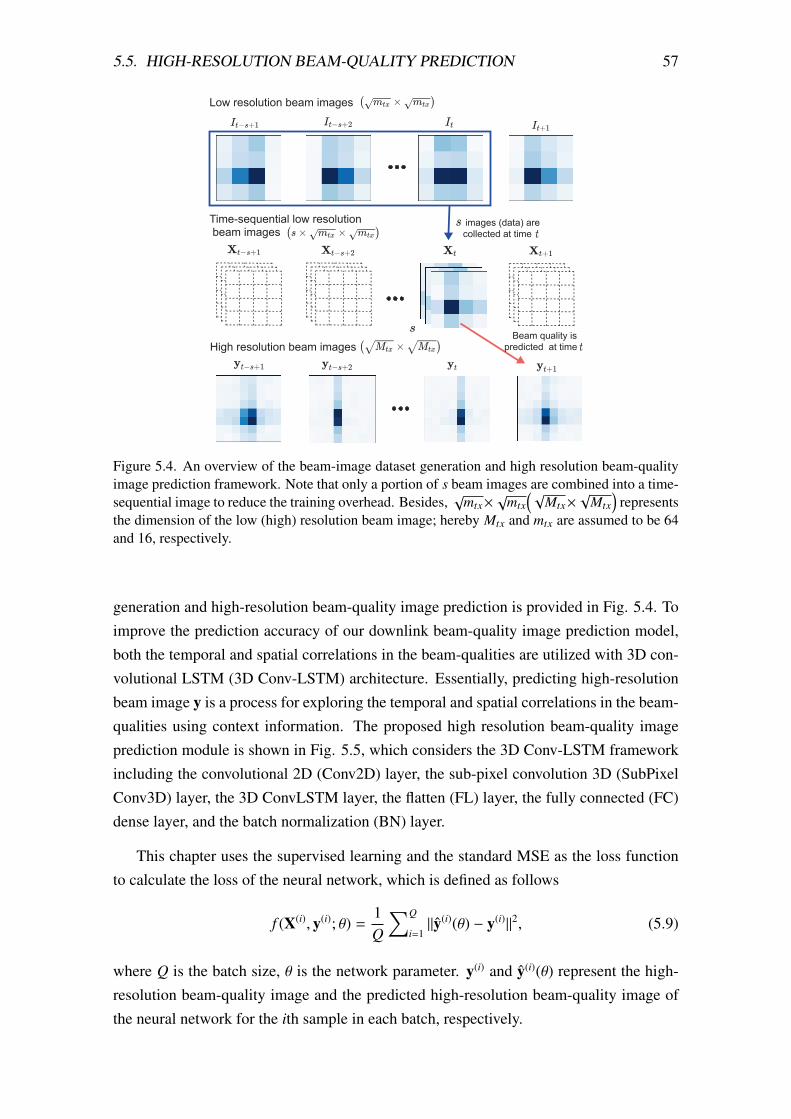
5.5. HIGH-RESOLUTION BEAM-QUALITY PREDICTION 57
Low resolution beam images
Time-sequential low resolution beam images
High resolution beam images
images (data) are
collected at time
collected at time collected at time
Beam quality is
predicted at time predicted at time
Figure 5.4. An overview of the beam-image dataset generation and high resolution beam-qualityimage prediction framework. Note that only a portion of s beam images are combined into a time-sequential image to reduce the training overhead. Besides,
√mtx×
√mtx
(√Mtx×
√Mtx
)represents
the dimension of the low (high) resolution beam image; hereby Mtx and mtx are assumed to be 64and 16, respectively.
generation and high-resolution beam-quality image prediction is provided in Fig. 5.4. Toimprove the prediction accuracy of our downlink beam-quality image prediction model,both the temporal and spatial correlations in the beam-qualities are utilized with 3D con-volutional LSTM (3D Conv-LSTM) architecture. Essentially, predicting high-resolutionbeam image y is a process for exploring the temporal and spatial correlations in the beam-qualities using context information. The proposed high resolution beam-quality imageprediction module is shown in Fig. 5.5, which considers the 3D Conv-LSTM frameworkincluding the convolutional 2D (Conv2D) layer, the sub-pixel convolution 3D (SubPixelConv3D) layer, the 3D ConvLSTM layer, the flatten (FL) layer, the fully connected (FC)dense layer, and the batch normalization (BN) layer.
This chapter uses the supervised learning and the standard MSE as the loss functionto calculate the loss of the neural network, which is defined as follows
f (X(i), y(i); θ) =1Q
∑Q
i=1‖y(i)(θ) − y(i)‖2, (5.9)
where Q is the batch size, θ is the network parameter. y(i) and y(i)(θ) represent the high-resolution beam-quality image and the predicted high-resolution beam-quality image ofthe neural network for the ith sample in each batch, respectively.

58 CHAPTER 5. BEAM AND POWER ALLOCATION USING DEEP LEARNING
Conv2D SubPixel
Conv3D
3DConv
LSTM
FL FCRelu
BN FCRelu
Input image data Output image
Figure 5.5. High-resolution beam-quality image prediction module.
Algorithm 3 Optimal Allocation Policy for Solving P2.
Input: Initialize the beam allocation policy uk,l,n; Initialize the beam combination set that collectsall the pairs {k, l}.
Output: The optimal beam and power allocation policy (U∗, p∗).1: for i = 1, · · · , I do2: Update the beam allocation policy ui
k,l,n and generate the possible beam combination setWi = {wi1 , · · · , wiK
}.
3: Update the power allocation vector pi by maximizing the introduced unconstrained La-grangian function in (5.11).
4: Calculate the sum-rate R(wi1 , · · · , wiK ) associated with the updated uik,l,n in Step 2 and the
updated pi in Step 3.
5: Compare the R(wi1 , · · · , wiK ) with the previous one until finding out the highest sum-rate.6: end for
5.6 Proposed Beam and Power Allocation
5.6.1 Optimal Allocation Solution
Note that the beam allocation is essentially the codeword allocation. The optimal beamallocation strategy is to calculate the sum rate in (5.8) for finding out the K differentcodewords exhaustively from the DFT-based codebookW. As such, the beam achievingthe largest sum rate is selected and then allocated for intended UE. More explicitly, theproposed algorithm is constituted by the following three major stages.
• Beam-allocation update: The total possible permutation of picking K differentbeams from the DFT-based codebook W is I = Mtx!
(Mtx−K)! . For the ith iteration, Iselect one possible beam combinationWi =
{wi1 , · · · , wiK
}, i ∈ {1, · · · , I}, as one
candidate beam set for K UEs, where wik means assigning the ikth beam to UEk ∈ {1, · · · ,K}.
• Power-allocation update: For the ith iteration, I update the downlink power allo-cation vector pi by solving the downlink power allocation problem of
maximizepi
R(wi1 , · · · , wiK ,pi
)s.t.
∑K
k=1pi,k ≤ Pmax. (5.10)
5.6. PROPOSED BEAM AND POWER ALLOCATION 59
Consider the following Lagrangian function
L (pi, µ) = R(wi1 , · · · , wiK ,pi
)− µ
(∑K
k=1pi,k − Pmax
)(5.11)
in which the introduced parameter µ > 0 indicates a Lagrangian multiplier.
Since the channel information is assumed to be unknown, estimating ‖hHk wik‖
2
seems to be rather difficult. Instead, I approximate ‖hHk wik‖
2 by applying the S-RNs and least-square (LS) estimator [106], based on the predicted received dataand known training signal. To this end, this chapter first predicts the received pow-er in real-part RR
k ∈ R√
Mtx×√
Mtx and the received power in imaginary-part RIk ∈
R√
Mtx×√
Mtx by exploiting the SRNs, thus resulting in Rk = RRk + jRI
k and Rk ∈
C√
Mtx×√
Mtx . Subsequently, this chapter estimates hHk wik by using the LS, based on
this predicted Rk. This chapter defines hk as the estimated channel vector betweenBS and UE k. Accordingly, it can be arrived at that vec(Rk) =
√pkhH
k wiks + nk,where pk denotes the transmit power preseted in beam-sweeping stage and pk > 0.By applying the LS estimator [106] and assuming that AoAs are accurately known,it is easy to arrive at
hHk wik =
s† · vec(Rk)√
pk. (5.12)
In such case, this chapter addresses the power allocation optimization problem in(5.10) by applying the Karush-Kuhn Tucker (KKT) conditions. From ∂L(pi, µ)
∂pi,k= 0,
it therefore arrives at
p∗i,k = max
1µ∗−
∑j,k pi, j‖hH
k wi j‖2 + N0
‖hHk wik‖
2, 0
. (5.13)
In addition, µ∗ can be obtained by exploiting the bisection search method under theother KKT condition
∑Kk=1 pi,k ≤ Pmax. In this way, the updated power allocation
vector pi = [p∗i,1, · · · , p∗i,K]T can be attained.
• Joint-allocation policy determination: Based on the above two stages, it is easyto obtain the combination of
(wi1 , · · · , wiK ,pi
)for each iteration of our algorith-
m. Accordingly, we can achieve the optimal beam and power allocation policy bysolving
(U∗,p∗) = arg maxi∈{1, ··· , I}
R(wi1 , · · · , wiK ,pi
). (5.14)
The procedure for solving this joint optimization problem P2 is summarized in Alg.1.Notably, the above approach assigns the best beam and power to UEs exhaustively bygoing through all the I = Mtx!
(Mtx−K)! possible beam combinations.

60 CHAPTER 5. BEAM AND POWER ALLOCATION USING DEEP LEARNING
Algorithm 4 Deep Learning-Based Allocation Policy for Solving P3.
Input: Initialize the beam allocation policy uk′,l′,n; Generate the time-sequential low resolutiondata X.
Output: The sub-optimal allocation policy (U∗1:K−γ,1:m,N , p∗).
1: Run the beam-quality prediction module with the low-resolution data X as input to learn thenetwork parameter θ until convergence.
2: Load the well-trained θ and re-predict the high-resolution beam qualities of a set of K UEs,and output their beam-quality lists. Pick the subset of γ UEs who have distinct strongestbeams, and the subset of K − γ UEs who share the same one or multiple strongest beams.
3: for i′ = 1, · · · , I′ do4: Update the ui′
k′,l′,n and the pi′ (based on the power allocation criteria in (5.13)).
5: Calculate R({wi′}I′i′=1,pi′) associated with the updated ui′
k′,l′,n and pi′ , and compareR({wi′}
I′i′=1,pi′) with the previous one until the highest one is met.
6: end for
Table 5.2
The Beam Confliction Probability for mmWaveMultiuser System with Typical mmWave Settings
Beam Selection ApproachMtx = 64, K = 8 Mtx = 64, K = 16
m = 20, γ = 2 m = 40, γ = 2 m = 20, γ = 4 m = 40, γ = 4
Exhaustive selection approach [82] 36.6 % 36.6 % 87.1 % 87.1 %
Top-m based approach 56.4 % 32.5 % 98.5 % 84.0 %
5.6.2 Deep Learning-Based Allocation Solution
Beam Confliction Probability
Proposition 5.6.1. Notably, the corresponding probability of selecting K different code-words from top-m beams without beam conflicts becomes
P (m, γ) =m!
mK−γ(m − K + γ)!, m ≥ K − γ. (5.15)
The beam confliction probability by using the top-m beam selection mechanism equalsto Pbc = 1 − P (m, γ). For ease of comparisons, TABLE 5.2 lists the Pbc (top-m basedapproach) and Pexh = 1 − Mtx!
MKtx(Mtx−K)! with Mtx � K (exhaustive selection approach)
for multiuser mmWave with a typical mmWave setting. Based on the results in TABLE5.2, this chapter deduces that (i) increasing the number of serving users will increase thebeam confliction probability, thus significantly deteriorating the system performance; (ii)increasing the number of top-m beams will decrease the beam confliction probability; (iii)The choice of m is critical for the deep learning-based solution, which in fact belongs toan accuracy and complexity trade-off.

5.7. EXPERIMENTAL RESULTS 61
Our Solution - The Design Rationale
To further reduce the overhead incurred for allocating the best beam and power in Alg.1,this chapter develops a sub-optimal allocation approach by exploiting the deep learningtechnology. The design rationale of our approach is to help BS make better allocationdecision while maintaining maximum sum-rate performance with low-overhead. Moreexplicitly, this chapter first invokes the beam-quality prediction model to predict the high-resolution beam image, and thus yielding a set of beam-quality lists. Such beam-qualitylist classes the Mtx beams in descending order from the strongest received power to thelowest received power (this chapter assumes that the strongest one is the most desiredbeam for each UE). In this way, this chapter assigns the strongest beam for each UE asthe preferred beam. However, for the multiuser mmWave system, some UEs’ locationmay co-located together, and thereby rendering that some of them may share the samebeam, thus causing severe beam conflicts. As such, this chapter finds out those UEs whohave the unique strongest beams based on their beam-quality lists. For ease of simplicity,this chapter assumes that there have γ UEs whose strongest beams are different, meaningthat K−γUEs share the same one or multiple strongest beams.2 Subsequently, this chaptersolves the beam allocation problem against those K−γ UEs by picking only top-m beamsfrom their beam-quality lists.
Our Solution - The Procedure Statement
Based on the aforementioned considerations, to allocate K different codewords from top-m beams without beam conflicts, this chapter therefore develops the following joint beam-assignment strategy and power allocation optimization problem (P3):
maximizeU, p
R({wi′}
I′i′=1,p
)(5.16a)
s.t.∑K−γ
k′=1uk′,l′,n ≤ 1 & uk′,l′,n ∈ {0, 1}, ∀ n, l′ ∈ {1, · · · ,m}, (5.16b)∑K
k=1pk ≤ Pmax, (5.16c)
where I′ = m!(m−K+γ)! refers to the total possible permutation of picking K − γ different
beams from the top-m beams. Note that the procedure for solving P3 is summarized inAlg.2.
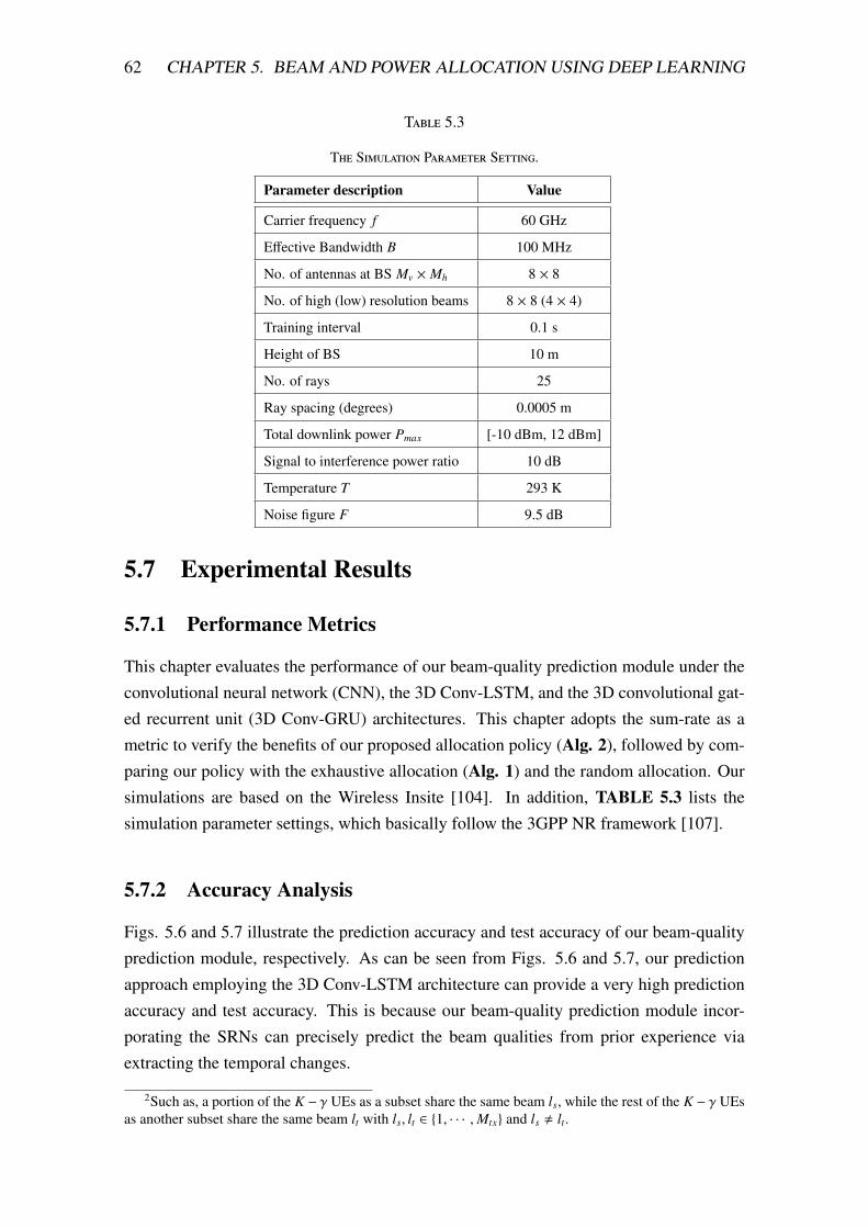
62 CHAPTER 5. BEAM AND POWER ALLOCATION USING DEEP LEARNING
Table 5.3
The Simulation Parameter Setting.
Parameter description Value
Carrier frequency f 60 GHz
Effective Bandwidth B 100 MHz
No. of antennas at BS Mv × Mh 8 × 8
No. of high (low) resolution beams 8 × 8 (4 × 4)
Training interval 0.1 s
Height of BS 10 m
No. of rays 25
Ray spacing (degrees) 0.0005 m
Total downlink power Pmax [-10 dBm, 12 dBm]
Signal to interference power ratio 10 dB
Temperature T 293 K
Noise figure F 9.5 dB
5.7 Experimental Results
5.7.1 Performance Metrics
This chapter evaluates the performance of our beam-quality prediction module under theconvolutional neural network (CNN), the 3D Conv-LSTM, and the 3D convolutional gat-ed recurrent unit (3D Conv-GRU) architectures. This chapter adopts the sum-rate as ametric to verify the benefits of our proposed allocation policy (Alg. 2), followed by com-paring our policy with the exhaustive allocation (Alg. 1) and the random allocation. Oursimulations are based on the Wireless Insite [104]. In addition, TABLE 5.3 lists thesimulation parameter settings, which basically follow the 3GPP NR framework [107].
5.7.2 Accuracy Analysis
Figs. 5.6 and 5.7 illustrate the prediction accuracy and test accuracy of our beam-qualityprediction module, respectively. As can be seen from Figs. 5.6 and 5.7, our predictionapproach employing the 3D Conv-LSTM architecture can provide a very high predictionaccuracy and test accuracy. This is because our beam-quality prediction module incor-porating the SRNs can precisely predict the beam qualities from prior experience viaextracting the temporal changes.
2Such as, a portion of the K − γ UEs as a subset share the same beam ls, while the rest of the K − γ UEsas another subset share the same beam lt with ls, lt ∈ {1, · · · ,Mtx} and ls , lt.

5.7. EXPERIMENTAL RESULTS 63
0 50 100 150 200 250 300epoch
0.65
0.70
0.75
0.80
0.85
0.90
0.95
Pred
ictio
n ac
cura
cy
Proposed scheme (3D Conv-LSTM) with s = 1Proposed scheme (3D Conv-LSTM) with s = 2Proposed scheme (3D Conv-LSTM) with s = 3
Figure 5.6. Prediction accuracy of our beam-quality prediction module employing the 3D Conv-LSTM architecture under various hyperparameter s = {1, 2, 3}.
0 50 100 150 200 250 300epoch
0.5
0.6
0.7
0.8
0.9
Test
acc
urac
y
Proposed scheme (3D Conv-LSTM) with s = 1Proposed scheme (3D Conv-LSTM) with s = 2Proposed scheme (3D Conv-LSTM) with s = 3
Figure 5.7. Test accuracy of our beam-quality prediction module employing the 3D Conv-LSTMarchitecture under various hyperparameter s = {1, 2, 3}.
Fig. 5.8 shows the MSE of the high-resolution beam quality y(i) and the predictedy(i)(θ) using our prediction approach. Fig. 5.8 reveals that the proposed approach employ-ing the CNN can converge faster than the proposed approach using other deep learningalgorithms. The reason behind is that CNN directly predicts the beam-quality based onthe simultaneous received power from UEs, thus facilitating a faster training per epoch.
5.7.3 Sum-Rate Performance
Fig. 5.9 depicts the sum-rate performance of different beam and power allocation ap-proaches with the perfect channel information. It is easy to see that Alg.2 can providealmost the same sum-rate performance as that of Alg.1. This indicates that the accuracyof our deep-learning based approach is reliable enough. On the other hand, comparing
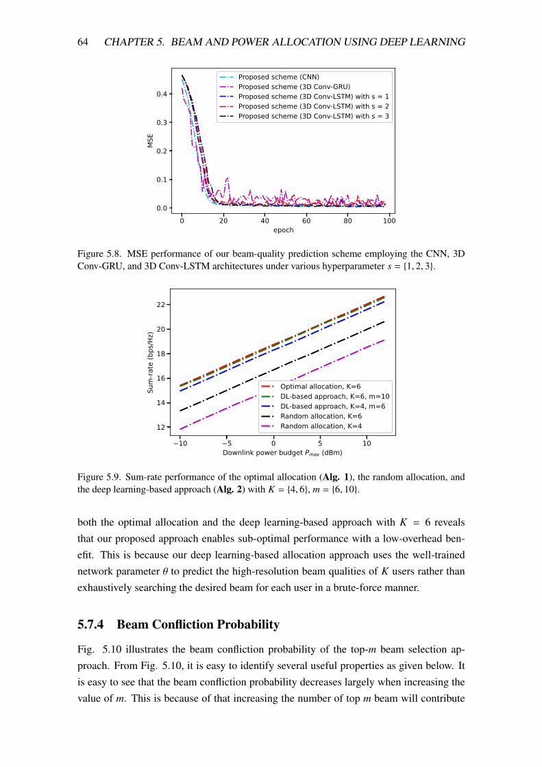
64 CHAPTER 5. BEAM AND POWER ALLOCATION USING DEEP LEARNING
0 20 40 60 80 100epoch
0.0
0.1
0.2
0.3
0.4
MSE
Proposed scheme (CNN)Proposed scheme (3D Conv-GRU)Proposed scheme (3D Conv-LSTM) with s = 1Proposed scheme (3D Conv-LSTM) with s = 2Proposed scheme (3D Conv-LSTM) with s = 3
Figure 5.8. MSE performance of our beam-quality prediction scheme employing the CNN, 3DConv-GRU, and 3D Conv-LSTM architectures under various hyperparameter s = {1, 2, 3}.
−10 −5 0 5 10Downlink power budget Pmax (dBm)
12
14
16
18
20
22
Sum
-rate
(bps
/Hz)
Optimal allocation, K=6DL-based approach, K=6, m=10DL-based approach, K=4, m=6Random allocation, K=6Random allocation, K=4
Figure 5.9. Sum-rate performance of the optimal allocation (Alg. 1), the random allocation, andthe deep learning-based approach (Alg. 2) with K = {4, 6}, m = {6, 10}.
both the optimal allocation and the deep learning-based approach with K = 6 revealsthat our proposed approach enables sub-optimal performance with a low-overhead ben-efit. This is because our deep learning-based allocation approach uses the well-trainednetwork parameter θ to predict the high-resolution beam qualities of K users rather thanexhaustively searching the desired beam for each user in a brute-force manner.
5.7.4 Beam Confliction Probability
Fig. 5.10 illustrates the beam confliction probability of the top-m beam selection ap-proach. From Fig. 5.10, it is easy to identify several useful properties as given below. Itis easy to see that the beam confliction probability decreases largely when increasing thevalue of m. This is because of that increasing the number of top m beam will contribute

5.8. CONCLUSION OF THIS CHAPTER 65
0 10 20 30 40 50 60 70
Top-m
0.7
0.75
0.8
0.85
0.9
0.95
1
Bea
m C
onfli
ctio
n P
roba
bilit
y
= 2 = 3 = 4 = 5 = 6 = 7
Figure 5.10. The beam confliction probability of the top-m selection approach with distinct (m, γ)configurations and K = 16.
to a better allocation performance, and thus decreasing the probability of beam conflicts.Moreover, it can also observe that higher (m, γ) configuration leads to lower beam conflic-tion probability. However, increasing the value of m will aggravate the beam and powerallocation complexity.
5.8 Conclusion of This Chapter
In summary, this chapter proposed a novel deep learning-based downlink beam and powerallocation approach for multiuser mmWave networks for facilitating a fast beamformingat the BS. More explicitly, this chapter first proposed a deep learning-based beam-qualityprediction model for predicting high-resolution beam qualities with low-overhead. Sub-sequently, this chapter developed a deep learning-based allocation approach which canprecisely assign the desired beam and power for UEs without beam conflicts. Simulationresults shown that our approach enables sub-optimal performance with a low-overheadbenefit.

66 CHAPTER 5. BEAM AND POWER ALLOCATION USING DEEP LEARNING

Chapter 6
Conclusions and Future Work
67

68 CHAPTER 6. CONCLUSIONS AND FUTURE WORK
The objective of this research is to develop advanced transmit precoding aided spatialmodulation approach and deep learning-based high-resolution beam-quality predictionapproach for guaranteeing high-quality and low latency mmWave communications. Tothis end, this dissertation first investigates the non-convex precoding optimization prob-lem as well as the non-convex problem solver. Based on this non-convex problem solver,this dissertation next proposes an OSD-aided scheme concentrating on the optimizationupon the precoding matrix, and a dual-ascent inspired transmit precoding design and ap-plication. Finally, this dissertation proposes a novel deep learning-based downlink beamand power allocation approach for multiuser mmWave networks for facilitating fast beam-forming at the BS.
6.1 Conclusions
In Chapter 2, I mainly focus on the non-convex precoding optimization problems as wellas how to solve this challenging optimization problem. To be concrete, this chapter gavedefinition of the transmit precoding design problem and the joint precoding weight opti-mization and power allocation problem. Next, this chapter analyzed the peculiarities ofthe above formulated non-convex optimization problems, followed by introducing someclassical solutions to the formulated non-convex optimization problems. In addition, thepros and cons of those solutions were discussed in this chapter.
In Chapter 4, an OSD-aided scheme was proposed to improve the performance of G-PSM systems under correlated fading channels. This chapter showed that the proposedschemes can achieve good BER performance compared to current simplified schemes.Especially, the proposed OSD-aided scheme is capable of providing significant BER per-formance improvement for GPSM systems, as well as facilitating low-complexity.
In Chapter 3, I developed dual-ascent inspired TPC techniques for the MASM-MIMOsystems. To tackle the challenging non-convex MMD and QCQP problems, this chap-ter proposed novel BFGS-DA scheme, and dual-ascent aided non-stationary TPC schemethat are capable of optimizing the precoding weights for all users. Subsequently, thischapter introduced an evolving MASM-MIMO system by imposing non-stationary time-varying TPC parameters. Simulation results revealed that our proposals are capable ofproviding significant BER performance improvement comparing with the existing meth-ods for MASM-MIMO. In addition, simulation results revealed that our proposals couldguarantee a larger d-min than the other existing d-min maximizing schemes proposed inearlier works. In particular, numerical results demonstrated the importance that our pro-posals possess an inherent robustness to the large-scale system dimension and quadraticconstraint.
In Chapter 5, I proposed a novel deep learning-based downlink beam and power al-location approach for multiuser mmWave networks for facilitating a fast beamforming at

6.2. FUTURE WORK 69
the BS. More explicitly, this chapter first proposed a deep learning-based beam-qualityprediction model for predicting high-resolution beam qualities with low-overhead. Sub-sequently, this chapter developed a deep learning-based allocation approach which canprecisely assign the desired beam and power for UEs without beam conflicts. Simulationresults shown that our approach enables sub-optimal performance with a low-overheadbenefit.
6.2 Future Work
For the future work, I mainly focus on designing superior codebook based beamformingapproach for guaranteeing near-optimal data rate performance while maintaining low-overhead benefit. In addition, I will try to further reduce the feedback-overhead by feed-ing back only top-n received signal reference power (RSRP) indices to BS. Hereby n isdefined as another hyperparameter to optimize.

70 CHAPTER 6. CONCLUSIONS AND FUTURE WORK

Appendix A
List of Author’s Publications andAwards
A.1 Journals
1. Y. Cao, T. Ohtsuki and T. Q. S. Quek, “Dual-Ascent Inspired Transmit Precod-ing for Evolving Multiple-Access Spatial Modulation,” in IEEE Transactions on
Communications, vol. 68, no. 11, pp. 6945-6961, Nov. 2020, doi: 10.1109/T-COMM.2020.3013030.
2. Y. Cao and T. Ohtsuki, “Spatial Degrees of Freedom Exploration and Analog Beam-forming Designs for Signature Spatial Modulation,” in IEICE TRANS. COMMUN.,VOL.E104B, NO.8 AUGUST 2021, doi: 10.1587/transcom.2020EBT0010.
3. H. Echigo, Y. Cao, M. Bouazizi and T. Ohtsuki, “A Deep Learning-Based LowOverhead Beam Selection in mmWave Communications,” in IEEE Transactions on
Vehicular Technology, vol. 70, no. 1, pp. 682-691, Jan. 2021, doi: 10.1109/TVT.2021.3049380.
4. Y. Cao and T. Ohtsuki, “Orthogonality Structure Designs for Generalized Precod-ing Aided Spatial Modulation,” in IEEE Wireless Communications Letters, vol. 8,no. 5, pp. 1406-1409, Oct. 2019, doi: 10.1109/LWC.2019.2919571.
5. Y. Cao, T. Ohtsuki and X. Jiang, “Precoding Aided Generalized Spatial ModulationWith an Iterative Greedy Algorithm,” in IEEE Access, vol. 6, pp. 72449-72457,2018, doi: 10.1109/ACCESS.2018.2880844.
6. Y. Cao, X. Jiang, H. Wang and E. Bai, “MIMO Wiretap Channels Based on Gener-alized Extended Orthogonal STBCs and Feedback,” in IEEE Transactions on Vehic-
ular Technology, vol. 67, no. 3, pp. 2454-2463, March 2018, doi: 10.1109/TVT.2017.2773527.
71

72 APPENDIX A. LIST OF AUTHOR’S PUBLICATIONS AND AWARDS
A.2 Full Articles on International Conferences Proceed-ings
1. Y. Cao, S. Maghsudi, and T. Ohtsuki, “Mobility-Aware Routing and Caching: AFederated Learning Assisted Approach,” in ICC 2021 - 2021 IEEE International
Conference on Communications (ICC), pp. 1-6, 2021.
2. Y. Cao and T. Ohtsuki, “Multi-Configuration Selection Mechanisms and AnalogPrecoding for Signature Spatial Modulation,” in ICC 2020 - 2020 IEEE Interna-
tional Conference on Communications (ICC), pp. 1-6, 2020.
3. Y. Cao and T. Ohtsuki, “Dual-Ascent Inspired Iterative Transmit Precoding Ap-proaches for Multiple Access Spatial Modulation,” in 2019 IEEE Global Commu-
nications Conference (GLOBECOM), pp. 1-6, 2019.
4. Y. Cao and T. Ohtsuki, “Precoding Aided Generalized Spatial Modulation with KTransmit Antenna Groups,” ICC 2019 - 2019 IEEE International Conference on
Communications (ICC), pp. 1-6, 2019.
5. Y. Cao, X. Jiang, M. Wen, E. Bai, Y. Wu and J. Li, “A new advantage distillationscheme over MIMO wiretap channels based on feedback bits,” 2017 14th IEEE
Annual Consumer Communications and Networking Conference (CCNC), pp. 628-629, 2017.
A.3 Articles on Domestic Conference Proceedings
1. Y. Cao and T. Ohtsuki, “Dual-Ascent Inspired Iterative Transmit Precoding Ap-proaches for Spatial Modulation in Multiple Access MIMO Systems,”, IEICE Gen-
eral Conf, Osaka Prefecture University, Jul. 2019.
A.4 Technical Reports
1. Y. Cao and T. Ohtsuki, “Mobility-Aware Routing and Caching in 5G Ultra-DenseNetworks”, IEICE RCS, pp. 1-5, Oct. 2020.
2. Y. Cao and T. Ohtsuki, “Spatial Degree of Freedom Exploration and Analog Beam-forming Designs for Signature Spatial Modulation”, IEICE RCS, pp. 1-5, Mar.2020.
3. Y. Cao and T. Ohtsuki, “BER Performance Optimization for Generalized SpatialModulation over Correlated Fading Channels”, IEICE RCS, pp. 1-5, Mar. 2019.

A.4. TECHNICAL REPORTS 73
4. Y. Cao and T. Ohtsuki, “Efficient Receive Antenna Subset Selection Algorithm forGeneralized Precoding Aided Spatial Modulation”, BCT, Feb. 2019.

74 APPENDIX A. LIST OF AUTHOR’S PUBLICATIONS AND AWARDS

References
[1] K. Poularakis, G. Iosifidis, V. Sourlas, and L. Tassiulas, “Exploiting caching andmulticast for 5G wireless networks,” IEEE Trans. Wireless Commun., vol. 15, no. 4,pp. 2995–3007, Apr. 2016.
[2] Y. Cao, S. Maghsudi, and T. Ohtsuki, “Mobility-aware routing and caching: Afederated learning assisted approach,” arXiv preprint arXiv:2102.10743, 2021.
[3] S. Maghsudi and M. van der Schaar, “A non-stationary bandit-learning approachto energy-efficient femto-caching with rateless-coded transmission,” IEEE Trans.
Wireless Commun., vol. 19, no. 7, pp. 5040–5056, Jul. 2020.
[4] N. Kato, B. Mao, F. Tang, Y. Kawamoto, and J. Liu, “Ten challenges in advanc-ing machine learning technologies toward 6G,” IEEE Wireless Communications,vol. 27, no. 3, pp. 96–103, Jun. 2020.
[5] B. Mao, Y. Kawamoto, and N. Kato, “Ai-based joint optimization of qos and secu-rity for 6g energy harvesting internet of things,” IEEE Internet of Things Journal,vol. 7, no. 8, pp. 7032–7042, Aug. 2020.
[6] S. Buzzi, C. I, T. E. Klein, H. V. Poor, C. Yang, and A. Zappone, “A survey ofenergy-efficient techniques for 5g networks and challenges ahead,” IEEE J. Sel.
Areas Commun., vol. 34, no. 4, pp. 697–709, Apr. 2016.
[7] T. Q. Dinh, J. Tang, Q. D. La, and T. Q. S. Quek, “Offloading in mobile edgecomputing: Task allocation and computational frequency scaling,” IEEE Trans.
Commun., vol. 65, no. 8, pp. 3571–3584, Aug. 2017.
[8] M. Wen, B. Zheng, K. J. Kim, M. Di Renzo, T. A. Tsiftsis, K.-C. Chen, and N. Al-Dhahir, “A survey on spatial modulation in emerging wireless systems: Researchprogresses and applications,” arXiv:1907.02941, Jul. 2019.
[9] M. Di Renzo, M. Debbah, D.-T. Phan-Huy, A. Zappone, M.-S. Alouini, C. Yuen,V. Sciancalepore et al., “Smart radio environments empowered by ai reconfigurablemeta-surfaces: An idea whose time has come,” arXiv:1903.08925, Mar. 2019.
75

76 REFERENCES
[10] P. Yang, Y. Xiao, M. Xiao, and S. Li, “6G wireless communications: Vision andpotential techniques,” IEEE Netw., vol. 33, no. 4, pp. 70–75, Jul. 2019.
[11] H. Echigo, Y. Cao, M. Bouazizi, and T. Ohtsuki, “A deep learning-based low over-head beam selection in mmwave communications,” IEEE Trans. Veh. Technol.,vol. 70, no. 1, pp. 682–691, Jan. 2021.
[12] B. Mao, F. Tang, Z. M. Fadlullah, N. Kato, O. Akashi, T. Inoue, and K. Mizu-tani, “A novel non-supervised deep-learning-based network traffic control methodfor software defined wireless networks,” IEEE Wireless Communications, vol. 25,no. 4, pp. 74–81, Aug. 2018.
[13] B. Mao, Z. M. Fadlullah, F. Tang, N. Kato, O. Akashi, T. Inoue, and K. Mizutani,“Routing or computing? the paradigm shift towards intelligent computer networkpacket transmission based on deep learning,” IEEE Transactions on Computers,vol. 66, no. 11, pp. 1946–1960, Nov. 2017.
[14] Y. Cao and T. Ohtsuki, “Orthogonality structure designs for generalized precodingaided spatial modulation,” IEEE Wireless Commun. Lett., vol. 8, no. 5, pp. 1406–1409, Oct. 2019.
[15] Y. Cao, T. Ohtsuki, and X.-Q. Jiang, “Precoding aided generalized spatial modula-tion with an iterative greedy algorithm,” IEEE Access, vol. 6, pp. 72 449–72 457,Nov. 2018.
[16] J. Jeganathan, A. Ghrayeb, and L. Szczecinski, “Spatial modulation: Optimal de-tection and performance analysis,” IEEE Commun. Lett., vol. 12, no. 8, pp. 545–547, Aug. 2008.
[17] M. D. Renzo, H. Haas, and P. M. Grant, “Spatial modulation for multiple-antennawireless systems: A survey,” IEEE Commun. Mag., vol. 49, no. 12, pp. 182–191,Dec. 2011.
[18] A. Younis, N. Serafimovski, R. Mesleh, and H. Haas, “Generalised spatial mod-ulation,” in 2010 Conference Record of the Forty Fourth Asilomar Conference on
Signals, Systems and Computers, Nov. 2010, pp. 1498–1502.
[19] E. Basar, “Index modulation techniques for 5g wireless networks,” IEEE Commun.
Mag., vol. 54, no. 7, pp. 168–175, Jul. 2016.
[20] E. Basar, U. Aygolu, E. Panayirci, and H. V. Poor, “Space-time block coded spatialmodulation,” IEEE Trans. Commun., vol. 59, no. 3, pp. 823–832, Mar. 2011.
[21] R. Mesleh, S. S. Ikki, and H. M. Aggoune, “Quadrature spatial modulation,” IEEE
Trans. Veh. Technol., vol. 64, no. 6, pp. 2738–2742, Jun. 2014.

REFERENCES 77
[22] Y. Cao, T. Ohtsuki, and T. Q. S. Quek, “Dual-ascent inspired transmit precodingfor evolving multiple-access spatial modulation,” IEEE Trans. Commun., vol. 68,no. 11, pp. 6945–6961, Nov. 2020.
[23] L. L. Yang, “Transmitter preprocessing aided spatial modulation for multiple-inputmultiple-output systems,” in Proc. IEEE Veh. Technol. Conf.-Spring, 2011, pp. 1–5.
[24] R. Zhang, L.-L. Yang, and L. Hanzo, “Generalised pre-coding aided spatial mod-ulation,” IEEE Trans. Wireless Commun., vol. 12, no. 11, pp. 5434 – 5443, Nov.2013.
[25] M. Zhang, M. Wen, X. Cheng, and L. Yang, “Pre-coding aided differential spatialmodulation,” in Proc. IEEE Global Commun. Conf. (GLOBECOM), 2015, pp. 1–6.
[26] J. Zheng, “Fast receive antenna subset selection for pre-coding aided spatial mod-ulation,” IEEE Wireless Commun. Lett., vol. 4, no. 3, pp. 317–320, Jun. 2015.
[27] P. Ju, M. Zhang, X. Cheng, C.-X. Wang, and L. Yang, “Generalized spatial modu-lation with transmit antenna grouping for correlated channels,” in Proc. IEEE ICC,May 2016, pp. 1 – 6.
[28] J. Li, M. Wen, X. Cheng, Y. Yan, S. Song, and M. H. Lee, “Generalized precoding-aided quadrature spatial modulation,” IEEE Trans. Veh. Technol., vol. 66, no. 2, pp.1881–1886, Feb. 2017.
[29] M. Wen, Q. Li, E. Basar, and W. Zhang, “Enhanced orthogonal frequency divi-sion multiplexing with index modulation,” IEEE Trans. Wireless Commun., vol. 16,no. 7, pp. 4786–4801, Jul. 2017.
[30] X.-Q. Jiang, M. Wen, J. Li, and W. Duan, “Distributed generalized spatial modula-tion based on chinese remainder theorem,” IEEE Commun. Lett., vol. 21, no. 7, pp.1501–1504, Jul. 2017.
[31] T. L. Narasimhan, P. Raviteja, and A. Chockalingam, “Generalized spatial mod-ulation in large-scale multiuser mimo systems,” IEEE Trans. Wireless Commun.,vol. 14, no. 7, pp. 3764 – 3779, Jul. 2015.
[32] Y. Xiao, S. Wang, L. Dan, X. Lei, P. Yang, and W. Xiang, “Ofdm with interleavedsubcarrier-index modulation,” IEEE Commun. Lett., vol. 18, no. 8, pp. 1447–1450,Aug. 2014.
[33] Y. Xiao, Z. Yang, L. Dan, P. Yang, L. Yin, and W. Xiang, “Low-complexity signaldetection for generalized spatial modulation,” IEEE Commun. Lett., vol. 18, no. 3,pp. 403–406, Mar. 2014.
78 REFERENCES
[34] S. Rangan, T. S. Rappaport, and E. Erkip, “Millimeter-wave cellular wireless net-works: Potentials and challenges,” Proc. IEEE, vol. 102, no. 3, pp. 366–385, Mar.2014.
[35] T. Nishio, H. Okamoto, K. Nakashima, Y. Koda, K. Yamamoto, M. Morikura,Y. Asai, and R. Miyatake, “Proactive received power prediction using machinelearning and depth images for mmwave networks,” IEEE J. Sel. Areas Commun.,vol. 37, no. 11, pp. 2413–2427, Nov. 2019.
[36] M. Xiao, S. Mumtaz, Y. Huang, L. Dai, Y. Li, M. Matthaiou, G. K. Karagiannidis,E. Bjornson, K. Yang, I. Chih-Lin et al., “Millimeter wave communications forfuture mobile networks,” IEEE J. Sel. Areas Commun., vol. 35, no. 9, pp. 1909–1935, Sep. 2017.
[37] Z. Xiao, T. He, P. Xia, and X.-G. Xia, “Hierarchical codebook design for beam-forming training in millimeter-wave communication,” IEEE Trans. Wirel. Com-
mun., vol. 15, no. 5, pp. 3380–3392, May 2016.
[38] D. Han and N. Lee, “Distributed precoding using local csit for mu-mimo heteroge-neous cellular networks,” IEEE Trans. Commun., Mar. 2021.
[39] E. Bjornson, L. Sanguinetti, J. Hoydis, and M. Debbah, “Designing multi-usermimo for energy efficiency: When is massive mimo the answer?” in 2014 IEEE
Wireless Communications and Networking Conference (WCNC), 2014, pp. 242–247.
[40] Y.-G. Lim, C.-B. Chae, and G. Caire, “Performance analysis of massive mimo forcell-boundary users,” IEEE Trans. Wireless Commun., vol. 14, no. 12, pp. 6827–6842, Dec. 2015.
[41] S. Rezaie, C. N. Manchon, and E. d. Carvalho, “Location- and orientation-aidedmillimeter wave beam selection using deep learning,” in 2020 IEEE International
Conference on Communications (ICC), 2020, pp. 1–6.
[42] Y. Yuan, G. Zheng, K.-K. Wong, B. Ottersten, and Z.-Q. Luo, “Transfer learn-ing and meta learning based fast downlink beamforming adaptation,” IEEE Trans.
Wireless Commun., Nov. 2020.
[43] X. Li and A. Alkhateeb, “Deep learning for direct hybrid precoding in millime-ter wave massive mimo systems,” in 2019 53rd Asilomar Conference on Signals,
Systems, and Computers, 2019, pp. 800–805.
REFERENCES 79
[44] W. Xia, G. Zheng, Y. Zhu, J. Zhang, J. Wang, and A. P. Petropulu, “A deep learningframework for optimization of miso downlink beamforming,” IEEE Trans. Com-
mun., vol. 68, no. 3, pp. 1866–1880, 2019.
[45] M. Joham, W. Utschick, and J. A. Nossek, “Linear transmit processing in mimocommunications systems,” IEEE Trans. Sig. Process., vol. 53, no. 8, pp. 2700–2712, Aug. 2005.
[46] M. Schubert and H. Boche, “Solution of the multiuser downlink beamformingproblem with individual sinr constraints,” IEEE Trans. Veh. Technol., vol. 53, no. 1,pp. 18–28, Jan. 2004.
[47] E. Visotsky and U. Madhow, “Space-time transmit precoding with imperfect feed-back,” IEEE transactions on Information Theory, vol. 47, no. 6, pp. 2632–2639,Sep. 2001.
[48] F. Khalid and J. Speidel, “Robust hybrid precoding for multiuser mimo wirelesscommunication systems,” IEEE transactions on wireless communications, vol. 13,no. 6, pp. 3353–3363, Jun. 2014.
[49] R. Irmer, A. N. Barreto, and G. Fettweis, “Transmitter precoding for spread-spectrum signals in frequency-selective fading channels,” in Proc. 3G Wireless,2001, pp. 939–944.
[50] P. Zetterberg, “Experimental investigation of tdd reciprocity-based zero-forcingtransmit precoding,” EURASIP Journal on Advances in Signal Processing, vol.2011, pp. 1–10, 2011.
[51] C. Windpassinger, R. F. Fischer, T. Vencel, and J. B. Huber, “Precoding in multi-antenna and multiuser communications,” IEEE Transactions on Wireless Commu-
nications, vol. 3, no. 4, pp. 1305–1316, Jul. 2004.
[52] A. Stavridis, S. Sinanovic, M. Di Renzo, and H. Haas, “Transmit precoding forreceive spatial modulation using imperfect channel knowledge,” in 2012 IEEE 75th
Vehicular Technology Conference (VTC Spring), 2012, pp. 1–5.
[53] O. El Ayach, R. W. Heath, S. Abu-Surra, S. Rajagopal, and Z. Pi, “Low complexityprecoding for large millimeter wave mimo systems,” in 2012 IEEE international
conference on communications (ICC), 2012, pp. 3724–3729.
[54] M. Vu and A. Paulraj, “Mimo wireless linear precoding,” IEEE Signal Processing
Magazine, vol. 24, no. 5, pp. 86–105, Sep. 2007.

80 REFERENCES
[55] F. Sohrabi, K. M. Attiah, and W. Yu, “Deep learning for distributed channel feed-back and multiuser precoding in fdd massive mimo,” IEEE Transactions on Wire-
less Communications, Jul. 2021.
[56] A. M. Elbir and A. K. Papazafeiropoulos, “Hybrid precoding for multiuser millime-ter wave massive mimo systems: A deep learning approach,” IEEE Transactions
on Vehicular Technology, vol. 69, no. 1, pp. 552–563, Jan. 2019.
[57] J.-M. Kang, I.-M. Kim, and C.-J. Chun, “Deep learning-based mimo-noma withimperfect sic decoding,” IEEE Systems Journal, vol. 14, no. 3, pp. 3414–3417,2019.
[58] H. Huang, Y. Song, J. Yang, G. Gui, and F. Adachi, “Deep-learning-basedmillimeter-wave massive mimo for hybrid precoding,” IEEE Transactions on Ve-
hicular Technology, vol. 68, no. 3, pp. 3027–3032, 2019.
[59] M. Ganji, H. Cheng, Q. Zhan, and K.-B. Song, “A new codebook design foranalog beamforming in millimeter-wave communication,” arXiv preprint arX-
iv:1902.00838, 2019.
[60] J. Wang, Z. Lan, C.-w. Pyo, T. Baykas, C.-s. Sum, M. A. Rahman, J. Gao, R. Fu-nada, F. Kojima, H. Harada et al., “Beam codebook based beamforming protocolfor multi-gbps millimeter-wave wpan systems,” IEEE Journal on Selected Areas in
Communications, vol. 27, no. 8, pp. 1390–1399, Oct. 2009.
[61] M. Alrabeiah and A. Alkhateeb, “Deep learning for mmwave beam and block-age prediction using sub-6 ghz channels,” IEEE Transactions on Communications,vol. 68, no. 9, pp. 5504–5518, Sep. 2020.
[62] A. Klautau, N. Gonzalez-Prelcic, and R. W. Heath, “Lidar data for deep learning-based mmwave beam-selection,” IEEE Wireless Communications Letters, vol. 8,no. 3, pp. 909–912, Jun. 2019.
[63] K. Satyanarayana, M. El-Hajjar, A. A. Mourad, and L. Hanzo, “Deep learningaided fingerprint-based beam alignment for mmwave vehicular communication,”IEEE Transactions on Vehicular Technology, vol. 68, no. 11, pp. 10 858–10 871,Nov. 2019.
[64] A. Alkhateeb, S. Alex, P. Varkey, Y. Li, Q. Qu, and D. Tujkovic, “Deep learning co-ordinated beamforming for highly-mobile millimeter wave systems,” IEEE Access,vol. 6, pp. 37 328–37 348, Jul. 2018.
[65] Y. Wang, M. Narasimha, and R. W. Heath, “Mmwave beam prediction with situa-tional awareness: A machine learning approach,” in 2018 IEEE 19th International

REFERENCES 81
Workshop on Signal Processing Advances in Wireless Communications (SPAWC),2018, pp. 1–5.
[66] C. Anton-Haro and X. Mestre, “Learning and data-driven beam selection formmwave communications: An angle of arrival-based approach,” IEEE Access,vol. 7, pp. 20 404–20 415, Feb. 2019.
[67] P. Yang, M. D. Renzo, Y. Xiao, S. Li, and L. Hanzo, “Design guidelines for spatialmodulation,” IEEE Commun. Surveys Tuts., vol. 17, no. 1, pp. 6–26, 1st Quart.2015.
[68] P. Yang, Y. L. Guan, Y. Xiao, M. Di Renzo, S. Li, and L. Hanzo, “Transmit precod-ed spatial modulation: Maximizing the minimum euclidean distance versus min-imizing the bit error ratio,” IEEE Trans. Wireless Commun., vol. 15, no. 3, pp.2054–2068, Mar. 2016.
[69] M. Lee, W. Chung, and T. Lee, “Generalized precoder design formulation anditerative algorithm for spatial modulation in mimo systems with csit,” IEEE Trans.
Commun., vol. 63, no. 4, pp. 1230–1244, Apr. 2015.
[70] P. Wang, Y. Li, L. Song, and B. Vucetic, “Multi-gigabit millimeter wave wirelesscommunications for 5G: From fixed access to cellular networks,” IEEE Commun.
Mag., vol. 53, no. 1, pp. 168–178, Jan. 2015.
[71] L. Wei, Q. Li, and G. Wu, “Exhaustive, iterative and hybrid initial access tech-niques in mmwave communications,” in 2017 IEEE Wireless Communications and
Networking Conference (WCNC), 2017, pp. 1–6.
[72] M. Giordani, M. Mezzavilla, C. N. Barati, S. Rangan, and M. Zorzi, “Comparativeanalysis of initial access techniques in 5G mmwave cellular networks,” in In Proc.
of 2016 50th Annu. Conf. Inf. Syst. Sci. CISS 2016, 2016, pp. 268–273.
[73] V. Va, H. Vikalo, and R. W. Heath, “Beam tracking for mobile millimeter wavecommunication systems,” in In Proc. of 2016 IEEE Glob. Conf. Signal Inf. Process.
Glob. 2016 - Proc., 2016, pp. 743–747.
[74] C.-H. Lin, W.-C. Kao, S.-Q. Zhan, and T.-S. Lee, “Bsnet: A deep learning-basedbeam selection method for mmwave communications,” in 2019 IEEE 90th Vehicu-
lar Technology Conference (VTC2019-Fall), 2019, pp. 1–6.
[75] X. Wang, X. Zhu, and Z. Sha, “A low-complexity iterative transmit precoding al-gorithm for spatial modulation systems,” in IEEE 87th Vehicular Technology Con-
ference (VTC Spring), May 2018, pp. 1–5.

82 REFERENCES
[76] M.-C. Lee and W.-H. Chung, “Adaptive multimode hybrid precoding for single-RF virtual space modulation with analog phase shift network in MIMO systems,”IEEE Trans. Wireless Commun., vol. 16, no. 4, pp. 2139–2152, Apr. 2017.
[77] M. Lee and W. Chung, “Transmitter design for analog beamforming aided spatialmodulation in millimeter wave MIMO systems,” in 2016 IEEE 27th Annual In-
ternational Symposium on Personal, Indoor, and Mobile Radio Communications
(PIMRC), Sep. 2016, pp. 1–6.
[78] S. Guo, H. Zhang, P. Zhang, P. Zhao, L. Wang, and M. Alouini, “Generalizedbeamspace modulation using multiplexing: A breakthrough in mmWave MIMO,”IEEE J. Sel. Areas Commun., vol. 37, no. 9, pp. 2014–2028, Sep. 2019.
[79] S. Sugiura, T. Ishihara, and M. Nakao, “State-of-the-art design of index modulationin the space, time, and frequency domains: Benefits and fundamental limitations,”IEEE Access, vol. 5, pp. 21 774–21 790, Oct. 2017.
[80] S. Boyd and L. Vandenberghe, Convex optimization. UK: Cambridge Uni. Press,2004.
[81] S. Timotheou and I. Krikidis, “Fairness for non-orthogonal multiple access in 5Gsystems,” IEEE Signal Process. Lett., vol. 22, no. 10, pp. 1647–1651, Oct. 2015.
[82] C. Jeong, J. Park, and H. Yu, “Random access in millimeter-wave beamformingcellular networks: Issues and approaches,” IEEE Commun. Mag., vol. 53, no. 1,pp. 180–185, Jan. 2015.
[83] G. Zheng, “Joint beamforming optimization and power control for full-duplex MI-MO two-way relay channel,” IEEE Trans. Signal Process., vol. 63, no. 3, pp. 555–566, Dec. 2014.
[84] L. Salaun, C. S. Chen, and M. Coupechoux, “Optimal joint subcarrier and powerallocation in NOMA is strongly NP-hard,” in 2018 IEEE International Conference
on Communications (ICC), 2018, pp. 1–7.
[85] E. Torkildson, U. Madhow, and M. Rodwell, “Indoor millimeter wave MIMO: Fea-sibility and performance,” IEEE Trans. Wireless Commun., vol. 10, no. 12, pp.4150–4160, 2011.
[86] L. Lu, G. Y. Li, A. L. Swindlehurst, A. Ashikhmin et al., “An overview of mas-sive mimo: benefits and challenges,” IEEE Journal of Selected Topics in Signal
Processing, vol. 8, no. 5, pp. 742–758, Oct. 2014.
[87] R. Mesleh, H. Haas, S. Sinanovic, C. W. Ahn, and S. Yun, “Spatial modulation,”IEEE Trans. Veh. Technol., vol. 57, no. 4, pp. 2228–2241, Jul. 2008.
REFERENCES 83
[88] M. D. Renzo, H. Haas, A. Ghrayeb, S. Sugiura, and L. Hanzo, “Spatial modula-tion for generalized mimo: Challenges, opportunities, and implementation,” Proc.
IEEE, vol. 102, no. 1, pp. 56–103, Jan. 2014.
[89] A. Stavridis, D. Basnayaka, S. Sinanovic, M. Di Renzo, and H. Haas, “A virtu-al mimo dual-hop architecture based on hybrid spatial modulation,” IEEE Trans.
Commun., vol. 62, no. 9, pp. 3161–3179, Sep. 2014.
[90] M. Koca and H. Sari, “Precoding for spatial modulation against correlated fadingchannels,” IEEE Trans. Wireless Commun., vol. 17, no. 9, pp. 5857–5870, Sep.2018.
[91] A. Younis, N. Serafimovski, R. Mesleh, and H. Haas, “Generalised spatial modu-lation,” in Proc. IEEE Asilomar Conf. on Signals, Syst. Comput., Nov. 2010, pp.1498–1502.
[92] S. K. Sharma, S. Chatzinotas et al., “Snr estimation for multi-dimensional cognitivereceiver under correlated channel/noise,” IEEE Trans. Wireless Commun., vol. 12,no. 12, pp. 6392–6405, Dec. 2013.
[93] S. Chatzinotas, M. A. Imran, and R. Hoshyar, “On the multicell processing capacityof the cellular mimo uplink channel in correlated rayleigh fading environment,”IEEE Trans. Wireless Commun., vol. 8, no. 7, pp. 3704–3715, Jul. 2009.
[94] Y. Cao and T. Ohtsuki, “Precoding aided generalized spatial modulation with Ktransmit antenna groups,” in Proc. IEEE Conference on Communications (ICC),2019, pp. 1–6, to appear.
[95] R. Rajashekar, K. V. S. Hari, and L. Hanzo, “Transmit antenna subset selection forsingle and multiuser spatial modulation systems operating in frequency selectivechannels,” IEEE Trans. Veh. Technol., vol. 67, no. 7, pp. 6156–6169, Jul. 2018.
[96] C. Downey, S. Narayanan, and M. F. Flanagan, “On generalized spatial modula-tion for multiuser wireless communications,” in 2017 14th IEEE Annual Consumer
Communications Networking Conference (CCNC), Jan. 2017, pp. 968–973.
[97] B. Hassibi and B. M. Hochwald, “How much training is needed in multiple-antennawireless links?” IEEE Trans. Inf. Theory, vol. 49, no. 4, pp. 951–963, Apr. 2003.
[98] Q. Li, D. Gesbert, and N. Gresset, “Cooperative channel estimation for coordinat-ed transmission with limited backhaul,” IEEE Trans. Wireless Commun., vol. 16,no. 6, pp. 3688–3699, Jun. 2017.
84 REFERENCES
[99] P. Yang, Y. Xiao, S. Li, and L. Hanzo, “A low-complexity power allocation algo-rithm for multiple-input multiple-output spatial modulation systems,” IEEE Trans.
Veh. Technol., vol. 65, no. 3, pp. 1819–1825, Mar. 2016.
[100] C. Masouros and L. Hanzo, “Constellation randomization achieves transmit diver-sity for single-rf spatial modulation,” IEEE Trans. Veh. Technol., vol. 65, no. 10,pp. 8101–8111, Oct. 2016.
[101] P. Cheng, Z. Chen, J. A. Zhang, Y. Li, and B. Vucetic, “A unified precoding schemefor generalized spatial modulation,” IEEE Trans. Commun., vol. 66, no. 6, pp.2502–2514, Jun. 2018.
[102] A. Skajaa, Limited memory BFGS for nonsmooth optimization. M.S. thesis, Dept.Comput. Sci. Math., Courant Inst. Math. Sci., New York, NY, USA, 2010.
[103] P. Ju, M. Zhang, X. Cheng, C. Wang, and L. Yang, “Generalized spatial modulationwith transmit antenna grouping for correlated channels,” in 2016 IEEE Internation-
al Conference on Communications (ICC), May 2016, pp. 1–6.
[104] Remcom. wireless insite. accessed: Jun. 27, 2018. [Online]. Available:http://www.remcom.com/wireless-insite
[105] J. Caballero, C. Ledig, A. Aitken, A. Acosta, J. Totz, Z. Wang, and W. Shi, “Real-time video super-resolution with spatio-temporal networks and motion compensa-tion,” in Proc. - 30th IEEE Conf. Comput. Vis. Pattern Recognition, CVPR 2017,2017, pp. 4778–4787.
[106] A. Khlifi and R. Bouallegue, “Performance analysis of LS and LMMSE channel es-timation techniques for LTE downlink systems,” arXiv preprint arXiv:1111.1666,2011.
[107] M. Giordani, M. Polese, A. Roy, D. Castor, and M. Zorzi, “A tutorial on beammanagement for 3GPP NR at mmwave frequencies,” IEEE Commun. Surv. Tut.,vol. 21, no. 1, pp. 173–196, 1st quarter, 2019.
Related Documents