A study on fuzzy clustering for magnetic resonance brain image segmentation using soft computing approaches

Page 1

As

Sa

b

a

ARRAA

KFKGPB

1

igigosmfg

atcIm

(

h1

Applied Soft Computing 24 (2014) 522–533

Contents lists available at ScienceDirect

Applied Soft Computing

j ourna l ho me page: www.elsev ier .com/ locate /asoc

study on fuzzy clustering for magnetic resonance brain imageegmentation using soft computing approaches

anjay Agrawala, Rutuparna Pandaa,∗, Lingraj Dorab

Department of Electronics & Telecommunication Engineering, VSS University of Technology, Burla 768018, IndiaDepartment of Electrical &Electronics Engineering, VSS University of Technology, Burla 768018, India

r t i c l e i n f o

rticle history:eceived 21 February 2013eceived in revised form 2 July 2014ccepted 6 August 2014vailable online 15 August 2014

eywords:uzzy C-means (FCM) clustering-means clusteringenetic algorithm (GA)article swarm optimization (PSO)acteria foraging optimization (BFO)

a b s t r a c t

This paper presents a novel idea of intracranial segmentation of magnetic resonance (MR) brain imageusing pixel intensity values by optimum boundary point detection (OBPD) method. The newly proposed(OBPD) method consists of three steps. Firstly, the brain only portion is extracted from the whole MRbrain image. The brain only portion mainly contains three regions–gray matter (GM), white matter (WM)and cerebrospinal fluid (CSF). We need two boundary points to divide the brain pixels into three regionson the basis of their intensity. Secondly, the optimum boundary points are obtained using the newlyproposed hybrid GA–BFO algorithm to compute final cluster centres of FCM method. For a comparison,other soft computing techniques GA, PSO and BFO are also used. Finally, FCM algorithm is executed onlyonce to obtain the membership matrix. The brain image is then segmented using this final membershipmatrix. The key to our success is that we have proposed a technique where the final cluster centres for FCMare obtained using OBPD method. In addition, reformulated objective function for optimization is used.Initial values of boundary points are constrained to be in a range determined from the brain dataset. The

boundary points violating imposed constraints are repaired. This method is validated by using simulatedT1-weighted MR brain images from IBSR database with manual segmentation results. Further, we haveused MR brain images from the Brainweb database with additional noise levels to validate the robustnessof our proposed method. It is observed that our proposed method significantly improves segmentationresults as compared to other methods.

© 2014 Elsevier B.V. All rights reserved.

. Introduction

Image segmentation has been a very critical and important stage in anymage processing application. It deals with dividing the pixels in an image intoroups or regions having similar features or characteristics for effective objectdentification. The segmentation of magnetic resonance (MR) brain image hasot significant focus in the field of biomedical image processing. Segmentationf MR brain image has got wide application in the field of bio-medical analysis,uch as identification of tumours, classification of tissues and blood cells, multiodal registration [1] etc. There are various segmentation techniques proposed

or MR brain image like thresholding [2], edge based detection [3] and regionrowing [4].

Thresholding techniques are effectively used when the histograms of the objectsnd background are clearly identifiable. But for brain image, these techniques give

he inaccurate segmentation result as distribution of pixels in brain image is veryomplex. Edge based methods rely heavily on detection of boundaries in the image.t is observed in the brain image that gray level distribution of pixels of gray

atter (GM), white matter (WM) and cerebrospinal fluid (CSF) result in incorrect

∗ Corresponding author. Tel.: +91 6632431857; fax: +91 6632430204.E-mail addresses: agrawals [email protected] (S. Agrawal), r [email protected]

R. Panda), [email protected] (L. Dora).

ttp://dx.doi.org/10.1016/j.asoc.2014.08.011568-4946/© 2014 Elsevier B.V. All rights reserved.

detection of boundary. Region growing techniques use the homogeneity and con-nectivity criteria for segmentation. It is not effectively used for brain imagesegmentation as the brain image does not contain well defined regions. The abovemethods are found effective for relatively simple images.

So one of the efficient techniques used for complex brain image segmentationis clustering. It classifies the pixels into larger groups depending on certain criteria.Again, several types of clustering methods have been discussed in literature likeExpectation–maximization [5], hard C-means, K-means and fuzzy clustering tech-niques [6]. Among fuzzy clustering techniques, fuzzy C-means (FCM) is the mostwidely used technique [7,8]. It aims at minimizing an objective function accordingto some criteria. It permits one data point to belong to more than one cluster definedby a membership matrix. But the random selection of centroids makes the techniquefall into local optimum. To overcome this problem, soft computing approaches likegenetic algorithm (GA) [9–11], Particle swarm optimization (PSO) [12], ant colonyoptimization (ACO) [13] etc. have been applied to improve FCM. Castillo et al. [14]presented optimization of the FCM algorithm by using evolutionary methods. Theyused GA and PSO only. They used it to find the optimal number of clusters and theweight exponent for different types of synthetic datasets. They emphasized on clus-ter validation. Hruschka et al. [15] presented a survey of evolutionary algorithms for

clustering. They emphasized on partition algorithms that focused on hard clusteringof data. The survey did not use any particular evolutionary method, but focused onadvanced topics like multi-objective and ensemble based evolutionary clustering.Then a taxonomy that highlights on some very important aspects of evolutionaryclustering was presented at the end.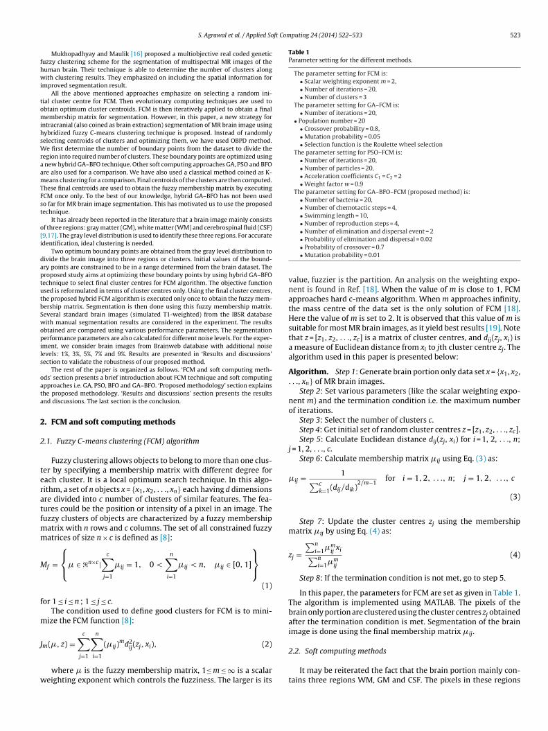

Page 2

ft Computing 24 (2014) 522–533 523

fhwi

tomihsWraamTFst

o[i

daptutbSwopils

oata

2

2

teratfmm

M

f

m

J

w

Table 1Parameter setting for the different methods.

The parameter setting for FCM is:• Scalar weighting exponent m = 2,• Number of iterations = 20,• Number of clusters = 3

The parameter setting for GA–FCM is:• Number of iterations = 20,

• Population number = 20• Crossover probability = 0.8,• Mutation probability = 0.05• Selection function is the Roulette wheel selection

The parameter setting for PSO–FCM is:• Number of iterations = 20,• Number of particles = 20,• Acceleration coefficients C1 = C2 = 2• Weight factor w = 0.9

The parameter setting for GA–BFO–FCM (proposed method) is:• Number of bacteria = 20,• Number of chemotactic steps = 4,• Swimming length = 10,• Number of reproduction steps = 4,• Number of elimination and dispersal event = 2

S. Agrawal et al. / Applied So

Mukhopadhyay and Maulik [16] proposed a multiobjective real coded geneticuzzy clustering scheme for the segmentation of multispectral MR images of theuman brain. Their technique is able to determine the number of clusters alongith clustering results. They emphasized on including the spatial information for

mproved segmentation result.All the above mentioned approaches emphasize on selecting a random ini-

ial cluster centre for FCM. Then evolutionary computing techniques are used tobtain optimum cluster centroids. FCM is then iteratively applied to obtain a finalembership matrix for segmentation. However, in this paper, a new strategy for

ntracranial (also coined as brain extraction) segmentation of MR brain image usingybridized fuzzy C-means clustering technique is proposed. Instead of randomlyelecting centroids of clusters and optimizing them, we have used OBPD method.

e first determine the number of boundary points from the dataset to divide theegion into required number of clusters. These boundary points are optimized using

new hybrid GA–BFO technique. Other soft computing approaches GA, PSO and BFOre also used for a comparison. We have also used a classical method coined as K-eans clustering for a comparison. Final centroids of the clusters are then computed.

hese final centroids are used to obtain the fuzzy membership matrix by executingCM once only. To the best of our knowledge, hybrid GA–BFO has not been usedo far for MR brain image segmentation. This has motivated us to use the proposedechnique.

It has already been reported in the literature that a brain image mainly consistsf three regions: gray matter (GM), white matter (WM) and cerebrospinal fluid (CSF)9,17]. The gray level distribution is used to identify these three regions. For accuratedentification, ideal clustering is needed.

Two optimum boundary points are obtained from the gray level distribution toivide the brain image into three regions or clusters. Initial values of the bound-ry points are constrained to be in a range determined from the brain dataset. Theroposed study aims at optimizing these boundary points by using hybrid GA–BFOechnique to select final cluster centres for FCM algorithm. The objective functionsed is reformulated in terms of cluster centres only. Using the final cluster centres,he proposed hybrid FCM algorithm is executed only once to obtain the fuzzy mem-ership matrix. Segmentation is then done using this fuzzy membership matrix.everal standard brain images (simulated T1-weighted) from the IBSR databaseith manual segmentation results are considered in the experiment. The results

btained are compared using various performance parameters. The segmentationerformance parameters are also calculated for different noise levels. For the exper-

ment, we consider brain images from Brainweb database with additional noiseevels: 1%, 3%, 5%, 7% and 9%. Results are presented in ‘Results and discussions’ection to validate the robustness of our proposed method.

The rest of the paper is organized as follows. ‘FCM and soft computing meth-ds’ section presents a brief introduction about FCM technique and soft computingpproaches i.e. GA, PSO, BFO and GA–BFO. ‘Proposed methodology’ section explainshe proposed methodology. ‘Results and discussions’ section presents the resultsnd discussions. The last section is the conclusion.

. FCM and soft computing methods

.1. Fuzzy C-means clustering (FCM) algorithm

Fuzzy clustering allows objects to belong to more than one clus-er by specifying a membership matrix with different degree forach cluster. It is a local optimum search technique. In this algo-ithm, a set of n objects x = {x1, x2, . . ., xn} each having d dimensionsre divided into c number of clusters of similar features. The fea-ures could be the position or intensity of a pixel in an image. Theuzzy clusters of objects are characterized by a fuzzy membership

atrix with n rows and c columns. The set of all constrained fuzzyatrices of size n × c is defined as [8]:

f =

⎧⎨⎩� ∈ �n×c |

c∑j=1

�ij = 1, 0 <

n∑i=1

�ij < n, �ij ∈ [0, 1]

⎫⎬⎭

(1)

or 1 ≤ i ≤ n ; 1 ≤ j ≤ c.The condition used to define good clusters for FCM is to mini-

ize the FCM function [8]:

(�, z) =c∑ n∑

(� )md2(z , x ), (2)

m

j=1 i=1

ij ij j i

where � is the fuzzy membership matrix, 1≤ m ≤ ∞ is a scalareighting exponent which controls the fuzziness. The larger is its

• Probability of elimination and dispersal = 0.02• Probability of crossover = 0.7• Mutation probability = 0.01

value, fuzzier is the partition. An analysis on the weighting expo-nent is found in Ref. [18]. When the value of m is close to 1, FCMapproaches hard c-means algorithm. When m approaches infinity,the mass centre of the data set is the only solution of FCM [18].Here the value of m is set to 2. It is observed that this value of m issuitable for most MR brain images, as it yield best results [19]. Notethat z = [z1, z2, . . ., zc] is a matrix of cluster centres, and dij(zj, xi) isa measure of Euclidean distance from xi to jth cluster centre zj. Thealgorithm used in this paper is presented below:

Algorithm. Step 1: Generate brain portion only data set x = {x1, x2,. . ., xn} of MR brain images.

Step 2: Set various parameters (like the scalar weighting expo-nent m) and the termination condition i.e. the maximum numberof iterations.

Step 3: Select the number of clusters c.Step 4: Get initial set of random cluster centres z = [z1, z2, . . ., zc].Step 5: Calculate Euclidean distance dij(zj, xi) for i = 1, 2, . . ., n;

j = 1, 2, . . ., c.Step 6: Calculate membership matrix �ij using Eq. (3) as:

�ij = 1∑ck=1(dij/dik)

2/m−1for i = 1, 2, . . ., n; j = 1, 2, . . ., c

(3)

Step 7: Update the cluster centres zj using the membershipmatrix �ij by using Eq. (4) as:

zj =∑n

i=1�mij

xi∑ni=1�m

ij

(4)

Step 8: If the termination condition is not met, go to step 5.

In this paper, the parameters for FCM are set as given in Table 1.The algorithm is implemented using MATLAB. The pixels of thebrain only portion are clustered using the cluster centres zj obtainedafter the termination condition is met. Segmentation of the brainimage is done using the final membership matrix �ij.

2.2. Soft computing methods

It may be reiterated the fact that the brain portion mainly con-tains three regions WM, GM and CSF. The pixels in these regions

Page 3

524 S. Agrawal et al. / Applied Soft Com

hiitptmabcsnWttsaw

sHAi

z

z

wpm

F

wHatt

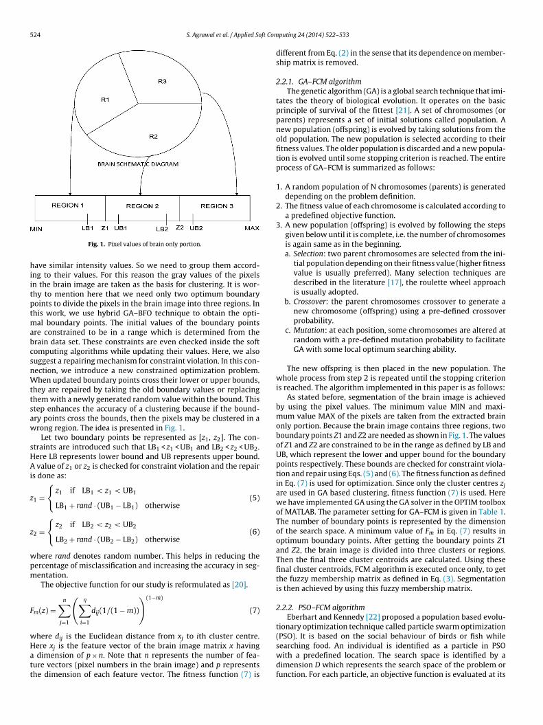
Fig. 1. Pixel values of brain only portion.

ave similar intensity values. So we need to group them accord-ng to their values. For this reason the gray values of the pixelsn the brain image are taken as the basis for clustering. It is wor-hy to mention here that we need only two optimum boundaryoints to divide the pixels in the brain image into three regions. Inhis work, we use hybrid GA–BFO technique to obtain the opti-

al boundary points. The initial values of the boundary pointsre constrained to be in a range which is determined from therain data set. These constraints are even checked inside the softomputing algorithms while updating their values. Here, we alsouggest a repairing mechanism for constraint violation. In this con-ection, we introduce a new constrained optimization problem.hen updated boundary points cross their lower or upper bounds,

hey are repaired by taking the old boundary values or replacinghem with a newly generated random value within the bound. Thistep enhances the accuracy of a clustering because if the bound-ry points cross the bounds, then the pixels may be clustered in arong region. The idea is presented in Fig. 1.

Let two boundary points be represented as [z1, z2]. The con-traints are introduced such that LB1 < z1 < UB1 and LB2 < z2 < UB2.ere LB represents lower bound and UB represents upper bound.

value of z1 or z2 is checked for constraint violation and the repairs done as:

1 ={

z1 if LB1 < z1 < UB1

LB1 + rand · (UB1 − LB1) otherwise(5)

2 ={

z2 if LB2 < z2 < UB2

LB2 + rand · (UB2 − LB2) otherwise(6)

here rand denotes random number. This helps in reducing theercentage of misclassification and increasing the accuracy in seg-entation.The objective function for our study is reformulated as [20].

m(z) =n∑

j=1

(�∑

i=1

dij(1/(1 − m))

)(1−m)

(7)

here dij is the Euclidean distance from xj to ith cluster centre.

ere xj is the feature vector of the brain image matrix x having

dimension of p × n. Note that n represents the number of fea-ure vectors (pixel numbers in the brain image) and p representshe dimension of each feature vector. The fitness function (7) is

puting 24 (2014) 522–533

different from Eq. (2) in the sense that its dependence on member-ship matrix is removed.

2.2.1. GA–FCM algorithmThe genetic algorithm (GA) is a global search technique that imi-

tates the theory of biological evolution. It operates on the basicprinciple of survival of the fittest [21]. A set of chromosomes (orparents) represents a set of initial solutions called population. Anew population (offspring) is evolved by taking solutions from theold population. The new population is selected according to theirfitness values. The older population is discarded and a new popula-tion is evolved until some stopping criterion is reached. The entireprocess of GA–FCM is summarized as follows:

1. A random population of N chromosomes (parents) is generateddepending on the problem definition.

2. The fitness value of each chromosome is calculated according toa predefined objective function.

3. A new population (offspring) is evolved by following the stepsgiven below until it is complete, i.e. the number of chromosomesis again same as in the beginning.a. Selection: two parent chromosomes are selected from the ini-

tial population depending on their fitness value (higher fitnessvalue is usually preferred). Many selection techniques aredescribed in the literature [17], the roulette wheel approachis usually adopted.

b. Crossover: the parent chromosomes crossover to generate anew chromosome (offspring) using a pre-defined crossoverprobability.

c. Mutation: at each position, some chromosomes are altered atrandom with a pre-defined mutation probability to facilitateGA with some local optimum searching ability.

The new offspring is then placed in the new population. Thewhole process from step 2 is repeated until the stopping criterionis reached. The algorithm implemented in this paper is as follows:

As stated before, segmentation of the brain image is achievedby using the pixel values. The minimum value MIN and maxi-mum value MAX of the pixels are taken from the extracted brainonly portion. Because the brain image contains three regions, twoboundary points Z1 and Z2 are needed as shown in Fig. 1. The valuesof Z1 and Z2 are constrained to be in the range as defined by LB andUB, which represent the lower and upper bound for the boundarypoints respectively. These bounds are checked for constraint viola-tion and repair using Eqs. (5) and (6). The fitness function as definedin Eq. (7) is used for optimization. Since only the cluster centres zjare used in GA based clustering, fitness function (7) is used. Herewe have implemented GA using the GA solver in the OPTIM toolboxof MATLAB. The parameter setting for GA–FCM is given in Table 1.The number of boundary points is represented by the dimensionof the search space. A minimum value of Fm in Eq. (7) results inoptimum boundary points. After getting the boundary points Z1and Z2, the brain image is divided into three clusters or regions.Then the final three cluster centroids are calculated. Using thesefinal cluster centroids, FCM algorithm is executed once only, to getthe fuzzy membership matrix as defined in Eq. (3). Segmentationis then achieved by using this fuzzy membership matrix.

2.2.2. PSO–FCM algorithmEberhart and Kennedy [22] proposed a population based evolu-

tionary optimization technique called particle swarm optimization(PSO). It is based on the social behaviour of birds or fish while

searching food. An individual is identified as a particle in PSOwith a predefined location. The search space is identified by adimension D which represents the search space of the problem orfunction. For each particle, an objective function is evaluated at its

Page 4

ft Com

cdipmta

blpt(clefi

v

x

wfi

ppv

p

Aet

of

t

t

Lamb

2

bbumf

b

d

S. Agrawal et al. / Applied So

urrent location. The particle, then moves in the search space with aynamically adjusted velocity according to its own experience and

ts neighbour’s experience thereby moving to a new location. Therocess is continued until all the particles in the population haveoved to their new locations. Finally, all the particles will move

o a location where an optimum value of the objective function ischieved.

Each particle in a population has a current location, a previousest location and a velocity. But the population has an overall best

ocation. The current location is assumed a problem solution. Therevious best location (i.e. location giving the best objective func-ion value) is identified as a variable pbest. The overall best locationi.e. location giving the best objective function value by any parti-le in the population) is identified as a variable gbest. The currentocation is continuously updated and new solutions are obtained byvaluating the objective function. The current locations are modi-ed by adding a dynamically adjusted velocity as given:

t+1 = w × vt + c1 × rand × (pbest − xt) + c2 × rand × (gbest − xt)

(8)

t+1 = xt + vt+1 (9)

here c1 and c2 represent acceleration constant, rand is the randomunction, w is the inertia weight, vt+1 is the updated velocity, xt+1s the updated current location of a particle.

It is compared with pbest and then pbest is updated. From thebest values, gbest value is evaluated. Thus, in PSO at each step, aarticle moves towards its pbest and gbest locations by updating itselocity.

The algorithm of PSO–FCM implemented for fuzzy clustering isresented below:

lgorithm. Step 1: Set the parameters of PSO, scalar weightingxponent m and stopping criteria as maximum number of itera-ions.

Step 2: Generate a swarm with P particles. Initialize the position xf particles which represent the number of boundary points. Checkor constraint violation and repair using Eqs. (5) and (6).

Step 3: Initialize velocity, pbest and gbest for the particles.Step 4: Calculate the fitness value for each particle using Eq. (7).Step 5: Calculate pbest value for each particle and gbest value for

he swarm.Step 6: Update the velocity of each particle using Eq. (8).Step 7: Update the position of each particle using Eq. (9) subject

o the constraints defined in Eqs. (5) and (6).Step 8: If the termination condition is not met, go to step 4.

In this paper, we have implemented the algorithm using MAT-AB. The stopping criterion is the maximum number of iterationsnd is taken as 20. The parameter setting is given in Table 1. Ainimum value of the fitness function in Eq. (7) gives us the final

oundary points.

.2.3. Hybrid GA–BFO–FCM algorithmPassino [23] proposed a nature inspired optimization algorithm

ased on the foraging technique of Escherichia coli bacteria. Theacteria searches for nutrients such that the energy obtained pernit time spent in searching is optimized or maximized. The move-ent of bacteria in this foraging technique has been discussed in

our important steps [24].

a) Chemotaxis: this step explains the movement of bacteria through

swimming and tumbling. A bacterium may swim or tumbledepending on the food concentration and environment condi-tion. If the condition is favourable then it continues to swimfor a pre-defined number of steps, otherwise it tumbles. These

puting 24 (2014) 522–533 525

two movement processes continue for the entire lifetime of thebacterium.

b) Swarming: during the process of foraging and maximizing theenergy obtained per unit time spent, the bacterium which hassearched the optimum path should attract the other bacteria bysending some signal. This will help the bacteria in concentratingthemselves as a swarm and move towards the optimum location.

c) Reproduction: this step shows the survival of the fittest charac-ter. The energy obtained per unit time spent for each bacteriumis sorted and the bacterium having the highest values aredeclared not healthy and hence die. The remaining bacteria areconsidered healthy and fit to reproduce (split into two) andare kept in the same location making the bacteria count same.Here we have used the crossover and mutation operation of GAto improve the result.

d) Elimination and dispersal: this step eliminates some bacteriadue to some disturbances in the environment like increase inheat killing the bacteria. This may also disperse some bacteriato a new location by change in condition like flow of water.

The algorithm for the above technique is presented as follows:

Step 1: Set the parameters of GA–BFO and scalar weighting expo-nent m.Step 2: Initialize the position P of each bacterium which representsthe boundary points. Check for constraint violation and repairusing Eqs. (5) and (6).Step 3: Increment the elimination–dispersal loop l = l + 1.Step 4: Increment the reproduction loop k = k + 1.Step 5: Increment the chemotaxis loop j = j + 1.

a. For each bacterium i a chemotactic step is taken as follows.. Calculate nutrient function J(i, j, k, l) for each bacterium.

c. Save Jlast = J(i, j, k, l) as better value may be obtained in the future.. Tumble: generate a random vector rand with each element in

[− 1, 1].e. Move: Let

P(i, j + 1, k, l) = P(i, j, k, l) + C(i) · rand(i)√randT (i) · rand(i)

This operation results in a step of size C(i) in the direction oftumble for bacterium i.

f. Calculate J(i, j + 1, k, l)g. Swim:

i. Initialize the counter for swim length = 0.ii. While counter less than the swimming length.

• Increment the counter.• If J(i, j + 1, k, l) < Jlast, let Jlast = J(i, j + 1, k, l). Update the position P

using the step size C(i) as

P(i, j + 1, k, l) = P(i, j + 1, k, l) + C(i) · rand(i)√randT (i) · rand(i)

and use this P to calculate the new J(i, j + 1, k, l) as in step (f).• Continue the above steps till counter equal the swimming length.

h. go to the next bacterium (i + 1) i.e. step 5b till all the bacteria areexhausted.

Step 6: If j < number of chemotactic steps, continue the chemotaxisloop and go to step 5.Step 7: Reproduction:

Page 5

526 S. Agrawal et al. / Applied Soft Computing 24 (2014) 522–533

ss for

a

b

d

e

nb

Mvpb

3

tmFii

Fig. 2. Block diagram of proce

. for given k, l and for each bacterium i let

Jihealth =

Nc+1∑j=1

J(i, j, k, l)

be the health of the bacteria i. Then sort the bacteria and thechemotactic parameter in ascending order of Jhealth.

. The bacteria with highest Jhealth values die and remaining bacte-ria with best values are treated as parent bacteria for the nextgeneration. However, in GA–BFO the idea of crossover mecha-nism from GA is used to search nearby locations by positioning50% of the bacteria randomly at different locations. We get somemore missing nutrients through the application of this process.In fact, GA–BFO supplements crossover feature of GA to generatebetter fitness function values.

c. Now two sets of parent bacteria are chosen and they crossoverwith a pre-defined crossover probability to get the offspringbacteria.

. Then the parent bacteria and the newly generated offspringbacteria are appended to form the original number of bacteriafor the next generation.

. A mutation of 1% is carried out to improvise results.

Step 8: If k < number of reproduction loop, continue the reproduc-tion loop and go to step 4.Step 9: Elimination – dispersal:

For a given probability of elimination and dispersal ped, elimi-ate or disperse each bacterium while keeping the population ofacteria constant.

Step 10: If l < elimination–dispersal loop, continue theelimination–dispersal loop and go to step 3. Otherwise endthe process.

In this paper, we have implemented GA–BFO algorithm withATLAB. The parameter setting is given in Table 1. A minimum

alue of the fitness function in Eq. (7) gives the final boundaryoints. The brain image is then segmented using the fuzzy mem-ership matrix as explained above.

. Proposed methodology

This section explains the proposed methodology of optimizinghe fuzzy clustering algorithm for intracranial MR brain image seg-

entation by using optimum boundary point detection (OBPD).uzzy clustering techniques reported earlier fall into local min-ma because of the random selection of centroids and resultsn inaccurate segmentation results. Here, an attempt is made

brain only portion extraction.

to overcome this problem using evolutionary computation (EC)approaches. The boundary points are optimized using various softcomputing approaches. Final centroids are obtained followed byclustering using the fuzzy membership matrix as in the FCM. TheMR brain image is then segmented using the cluster information.T1-weighted MR coronal slice taken from MRI data set of 20 normalsubjects with manual segmentation results (ground truth) availablein IBSR database are considered here to experiment [25].

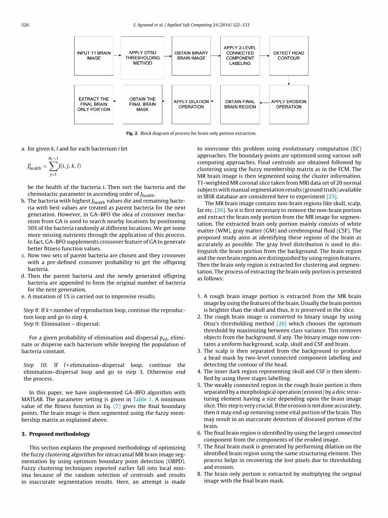
The MR brain image contains non-brain regions like skull, scalp,fat etc. [26]. So it is first necessary to remove the non-brain portionand extract the brain only portion from the MR image for segmen-tation. The extracted brain only portion mainly consists of whitematter (WM), gray matter (GM) and cerebrospinal fluid (CSF). Theproposed study aims at identifying these regions of the brain asaccurately as possible. The gray level distribution is used to dis-tinguish the brain portion from the background. The brain regionand the non brain region are distinguished by using region features.Then the brain only region is extracted for clustering and segmen-tation. The process of extracting the brain only portion is presentedas follows:

1. A rough brain image portion is extracted from the MR brainimage by using the features of the brain. Usually the brain portionis brighter than the skull and thus, it is preserved in the slice.

2. The rough brain image is converted to binary image by usingOtsu’s thresholding method [26] which chooses the optimumthreshold by maximizing between class variance. This removesobjects from the background, if any. The binary image now con-tains a uniform background, scalp, skull and CSF and brain.

3. The scalp is then separated from the background to producea head mask by two-level connected component labelling anddetecting the contour of the head.

4. The inner dark region representing skull and CSF is then identi-fied by using three stages labelling.

5. The weakly connected region in the rough brain portion is thenseparated by a morphological operation (erosion) by a disc struc-turing element having a size depending upon the brain imageslice. This step is very crucial. If the erosion is not done accurately,then it may end up removing some vital portion of the brain. Thismay result in an inaccurate detection of diseased portion of thebrain.

6. The final brain region is identified by using the largest connectedcomponent from the components of the eroded image.

7. The final brain mask is generated by performing dilation on theidentified brain region using the same structuring element. This

process helps in recovering the lost pixels due to thresholdingand erosion.

8. The brain only portion is extracted by multiplying the originalimage with the final brain mask.

Page 6

S. Agrawal et al. / Applied Soft Computing 24 (2014) 522–533 527

tractio

p

fp

t

tpath

stiatcEatvbrt

4

dtiwfl3

J = Igt ∩ Iseg

Igt ∪ Iseg(10)

Fig. 3. Brain only image ex

The block diagram for methodology of extraction of brain onlyortion is presented in Fig. 2.

T1-weighted MR coronal slice (slice no. 15 of Image 5 8) takenrom MRI data set of 20 normal subjects is presented to display therocess of extraction of brain only portion in Fig. 3.

After getting the final brain portion from above steps, segmen-ation is done by using OBPD method.

In this paper, the fitness function (7) does not consider any spa-ial dependence among the brain image matrix and each imageixel is considered as an individual point. The membership matrixs in Eq. (3) is determined by a measure of similarity betweenhe pixel intensity and cluster centroids. The membership value isigher when the intensity values are closer to the cluster centroids.

In our problem, the feature vectors xj represent the pixel inten-ity, its dimension p = 1. Here zi is the ith cluster centre, � representshe number of clusters and m is the scalar weighting constant ands taken as 2. The optimized boundary points computed from Eq. (7)re used to find the final cluster centres in the three regions. Usinghese final cluster centres, GA–BFO–FCM (proposed method) is exe-uted only once to obtain the fuzzy membership matrix of size n × c.ach term of the fuzzy membership matrix represents the extent ofssociation of jth object with ith cluster centre. The objects nearesto the centroids of their cluster are assigned a high membershipalue and objects far from these centroids are assigned low mem-ership value. So the pixels in the brain are segmented into threeegions according to their membership value. The block diagram forhe process of segmentation of brain image is presented in Fig. 4.

The flow chart of the proposed method is presented in Fig. 5.

. Results and discussions

Simulated T1-weighted MR coronal slice taken from MRI brainata sets from 20 normal subjects available in IBSR database withhe manual segmentation result are used to experiment. The MR

mages are acquired by 1.5 T General Electric Signa MR System (Mil-

aukee, WI), with the following parameters: TR = 50 ms, TE = 9 ms,ip angle = 50◦, field of view = 24 cm, slice thickness = contiguous.0 mm, matrix = 256 × 256.

n process from MR image.

The images are segmented using K-Means, FCM, GA–FCM,PSO–FCM, BFO–FCM and our proposed technique. It is important tonote that no readily available data for parameters is used for com-parison; we have implemented all techniques and generated datafor this work. In all the techniques, the fitness function defined inEq. (7) is used. The scalar weighting exponent m for all the methodsused is taken as 2. Results are displayed in the form of tables andfigures.

Results are compared using segmentation evaluation indiceslike Jaccard similarity index, Dice coefficient, false positive rate andfalse negative rate [27,30]. The Jaccard similarity index [28], alsoknown as the Tanimoto coefficient, is used to measure the simi-larity of two clusters. It is defined as the ratio of the number ofcommon pixels between the ground truth and segmented imageto the number of identical pixels of ground truth and segmentedimage:

Fig. 4. Block diagram for the proposed MR brain image segmentation method.

Page 7

528 S. Agrawal et al. / Applied Soft Computing 24 (2014) 522–533

wTho

la

D

Am

tcspi

f

a

f

wsg

may be noted that we deal with a simulated database with groundtruth. Hence, noise filtering is not required before the brain extrac-tion process. Here Table 2 shows the segmentation results with

Fig. 5. Flow chart of the proposed method.

here Igt is the ground truth image and Iseg is the segmented image.he Jaccard index is zero if the two clusters are disjoint, i.e. theyave no common pixels and one if they are identical. A higher valuef this index indicates better segmentation result.

The Dice coefficient [29] is another index like the Jaccard simi-arity index for measuring the similarity of two clusters. It is defineds [29]:

= 2 × Igt ∩ Iseg

Igt + Iseg(11)

higher value of the Dice coefficient indicates more accurate seg-entation.The false positive rate and the false negative rate are also used

o validate the clustering phenomenon. The false positive rate indi-ates the possibility of pixels belonging to a cluster, but is notegmented into that cluster. The false negative rate indicates theossibility of pixels not belonging to a cluster, but is segmented

nto that cluster. They are calculated as:

pr = Nseg − N(Igt + Iseg)Ngt

(12)

nd

nr = Ngt − N(Igt + Iseg)Ngt

(13)

here fpr is false positive rate, Nseg is the number of pixels in theegmented image, N(Igt + Iseg) is the number of pixels common toround truth and segmented image, Ngt is the number of pixels in

Fig. 6. Simulated T1 weighted slice 15 of MR Image 1 24.

the ground truth image and fnr is false negative rate. Lower valuesof these rates indicate better segmentation result.

The 15th slice of the brain only region of the simulated imageand its segmented results using the proposed method is shownin Figs. 6–10. The regions only show GM, WM and CSF. The back-ground pixels are removed during the brain extraction process. It

Fig. 7. Simulated T1 weighted slice 15 of MR Image 4 8.

Page 8

S. Agrawal et al. / Applied Soft Computing 24 (2014) 522–533 529

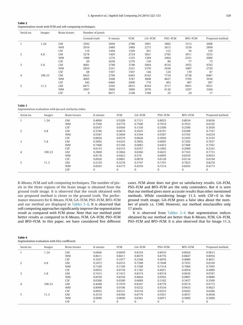
Table 2Segmentation result with FCM and soft computing techniques.

Serial no. Images Brain tissues Number of pixels

Ground truth K-means FCM GA–FCM PSO–FCM BFO–FCM Proposed method

1 1 24 GM 3592 2694 2788 3991 3802 3313 3608WM 2916 2489 2489 2275 2613 3258 2890CSF 119 1444 1350 361 212 56 129

2 4 8 GM 3278 1429 2724 3821 2782 3011 3252WM 1988 1276 1335 1384 2464 2251 2006CSF 69 2630 1276 130 89 77 73

3 5 8 GM 4681 3740 3740 5064 4516 3952 4762WM 2829 2331 2331 2370 2938 3487 2729CSF 68 1507 1507 144 124 139 87

4 100 23 GM 8423 2796 6443 8162 7710 6738 8487WM 4065 3568 3787 3898 4627 5705 3936CSF 342 6466 2600 770 493 407 387

5 11 3 GM 8471 2292 6815 8554 3717 9951 9551WM 3997 3909 3909 2978 9130 3297 3304CSF 0 6671 2148 1340 25 24 17

Table 3Segmentation evaluation with Jaccard similarity index.

Serial no. Images Brain tissues K-means FCM GA–FCM PSO–FCM BFO–FCM Proposed method

1 1 24 GM 0.4999 0.5209 0.7151 0.8025 0.8034 0.9636WM 0.7560 0.6776 0.7500 0.7819 0.7933 0.8102CSF 0.0547 0.0569 0.1330 0.2500 0.2560 0.3030

2 4 8 GM 0.3766 0.4874 0.5625 0.6191 0.6308 0.7167WM 0.5587 0.3604 0.5344 0.5587 0.5765 0.6254CSF 0.0026 0.0379 0.0628 0.3056 0.3293 0.3335

3 5 8 GM 0.5892 0.4325 0.5892 0.6095 0.7202 0.7837WM 0.7468 0.5160 0.6083 0.6453 0.7468 0.7561CSF 0.0153 0.0153 0.0357 0.1892 0.2090 0.2241

4 100 23 GM 0.2860 0.3864 0.6366 0.6625 0.7163 0.7753WM 0.8178 0.4423 0.579 0.6995 0.8359 0.9033CSF 0.0026 0.0061 0.0078 0.0128 0.0134 0.0194

5 11 3 GM 0.2129 0.3278 0.3747 0.7191 0.7823 0.827873

Kegomasrba

TS

WM 0.8263 0.41CSF 0 0

-Means, FCM and soft computing techniques. The number of pix-ls in the three regions of the brain image is obtained from theround truth image. It is observed that the result obtained withur proposed method is closer to the ground truth. The perfor-ance measures for K-Means, FCM, GA–FCM, PSO–FCM, BFO–FCM

nd our method are displayed in Tables 3–6. It is observed thatoft computing approaches significantly improve the segmentation

esult as compared with FCM alone. Note that our method yieldetter results as compared to K-Means, FCM, GA–FCM, PSO–FCMnd BFO–FCM. In this paper, we have considered five different

able 4egmentation evaluation with Dice coefficient.

Serial no. Images Brain tissues K-means FCM

1 1 24 GM 0.6666 0.6850

WM 0.8611 0.8611

CSF 0.1037 0.1077

2 4 8 GM 0.5472 0.6553

WM 0.7169 0.7169

CSF 0.0052 0.0730

3 5 8 GM 0.7415 0.7415

WM 0.8550 0.8550

CSF 0.0300 0.0300

4 100 23 GM 0.4448 0.7970

WM 0.8998 0.9106

CSF 0.0052 0.0121

5 11 3 GM 0.3510 0.8366

WM 0.9049 0.9049

CSF 0 0

0.4359 0.7214 0.8263 0.41730 0 0 0

cases. FCM alone does not give us satisfactory results. GA–FCM,PSO–FCM and BFO–FCM are the only contenders. But it is seenthat our method gives more accurate results than other mentionedmethods. While considering Image 11 3, with CSF = 0 in theground truth image, GA–FCM gives a false idea about the num-ber of pixels i.e. 1340. However, our method misclassifies only17 pixels.

It is observed from Tables 3–6 that segmentation indicesobtained by our method are better than K-Means, FCM, GA–FCM,PSO–FCM and BFO–FCM. It is also observed that for Image 11 3,

GA–FCM PSO–FCM BFO–FCM Proposed method

0.8339 0.8910 0.8924 0.98130.8679 0.8776 0.8847 0.89560.2348 0.4076 0.4080 0.46510.7200 0.7648 0.7935 0.83500.7298 0.7314 0.7966 0.79950.1182 0.4651 0.4954 0.49890.8374 0.8574 0.9039 0.97870.8844 0.9565 0.9807 0.98800.0689 0.3182 0.3457 0.35090.8347 0.8779 0.9574 0.97730.9232 0.9334 0.9433 0.98250.0154 0.0253 0.0265 0.02860.8779 0.5451 0.4937 0.49380.8381 0.6071 0.5889 0.58890 0 0 0

Page 9

530 S. Agrawal et al. / Applied Soft Computing 24 (2014) 522–533

Table 5Segmentation evaluation with false negative rate.

Serial no. Images Brain tissues K-means FCM GA–FCM PSO–FCM BFO–FCM Proposed method

1 1 24 GM 0.2223 0.3917 0.0966 0.0830 0.0589 0.0553WM 0.0651 0.4020 0.3086 0.1529 0.1142 0.1825CSF 0.9446 0.2121 0.1545 0.1457 0.1359 0.1349

2 4 8 GM 0.0987 0.4001 0.2205 0.2103 0.1379 0.1279WM 0.0831 0.4115 0.1378 0.1207 0.0820 0.0754CSF 0.9973 0.1774 0.1535 0.1377 0.1145 0.0973

3 5 8 GM 0.1652 0.3330 0.2284 0.2069 0.1653 0.0402WM 0.0536 0.2202 0.0085 0.0046 0.0025 0.0020CSF 0.9847 0.0417 0.0417 0.0416 0.0412 0.0405

4 100 23 GM 0.1077 0.2967 0.1782 0.1512 0.1043 0.0174WM 0.0376 0.1205 0.0950 0.0850 0.0520 0.0292CSF 0.9974 0.6364 0.6118 0.5318 0.4545 0.3897

5 11 3 GM 0.1758 0.2452 0.1178 0.6078 0.6571 0.1202WM 0.0849 0.1051 0.2687 0.0030 0.0020 0.0008CSF NaN NaN NaN NaN NaN NaN

Table 6Segmentation evaluation with false positive rate.

Serial no. Images Brain tissues K-means FCM GA–FCM PSO–FCM BFO–FCM Proposed method

1 1 24 GM 0.5557 0.1679 0.1634 0.1414 0.1105 0.1125WM 0.2366 0.0556 0.0202 0.0133 0.0116 0.0144CSF 0.0132 1.8485 1.1010 0.6970 0.6566 0.2300

2 4 8 GM 1.3933 0.2309 0.1858 0.0817 0.0589 0.0169WM 0.6411 0.0533 0.0050 0.0049 0.0027 0.0015CSF 0.0209 20.7097 11.8387 10.7419 10.3226 10.3073

3 5 8 GM 0.4168 0.1320 0.1102 0.0060 0.0051 0.0047WM 0.2673 0.0442 0.0095 0.0063 0.0032 0.0023CSF 0.0006 61.8333 25.8750 25.0833 21.7917 21.0432

4 100 23 GM 2.1202 0.0616 0.0472 0.0392 0.0241 0.0237WM 0.1768 0.0522 0.0279 0.0255 0.0203 0.0054CSF 0.0042 58.7273 39.9091 34.3182 32.3864 10.3400

5 11 3 GM 2.8717 0.0497 0.0476 0.0466 0.0463 1.6840WM 0.1074 0.0831 0.0138 1.2872 1.3915 0.5823CSF Inf Inf Inf Inf Inf Inf

Fig. 8. Simulated T1 weighted slice 15 of MR Image 5 8. Fig. 9. Simulated T1 weighted slice 15 of MR Image 11 3.

Page 10

S. Agrawal et al. / Applied Soft Com

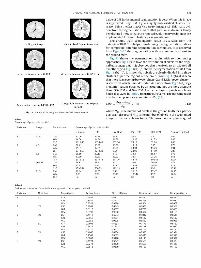
Fig. 10. Simulated T1 weighted slice 15 of MR Image 100 23.

Table 7Percentage of pixels misclassified.

Serial no. Images Brain tissues Percentage of pixels misclassi

K-means FCM

1 1 24 GM 25.00 22.38

WM 14.64 14.64

CSF 1113.45 1034.45

2 4 8 GM 56.41 16.90

WM 35.81 32.85

CSF 3711.59 1749.28

3 5 8 GM 20.10 20.10

WM 17.60 17.60

CSF 2116.18 2116.18

4 100 23 GM 66.81 23.51

WM 12.23 6.84

CSF 1790.64 660.23

5 11 3 GM 72.94 19.55

WM 2.20 2.20

CSF Inf Inf

Table 8Performance measures for noisy brain images with the proposed method.

Serial no. Noise level Brain tissues Jaccard index

1 0% CSF 0.4951

GM 0.8086

WM 0.9387

2 1% CSF 0.4869

GM 0.8110

WM 0.9398

3 3% CSF 0.4918

GM 0.7555

WM 0.9056

4 5% CSF 0.4808

GM 0.7687

WM 0.9126

5 7% CSF 0.4660

GM 0.7563

WM 0.9007

6 9% CSF 0.4521

GM 0.7271

WM 0.8812

puting 24 (2014) 522–533 531

value of CSF in the manual segmentation is zero. When this imageis segmented using FCM, it gives highly misclassified clusters. Thereason being the fact that CSF is zero for Image 11 3. This is also evi-dent from the segmentation indices that give unusual results. It maybe reiterated the fact that our proposed evolutionary techniques areimplemented for three clusters for segmentation.

The ground truth segmentation result is available from thedatasets of IBSR. This helps us in defining the segmentation indicesfor comparing different segmentation techniques. It is observedfrom Figs. 6–10 that segmentation with our method is closest tothe ground truth.

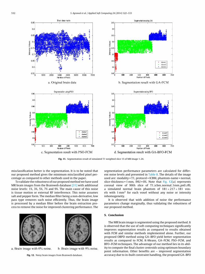
Fig. 11 shows the segmentation results with soft computingapproaches. Fig. 11(a) shows the distribution of pixels for the origi-nal brain image data. It is observed that the pixels are distributed allover the region. Fig. 11(b)–(d) shows the segmentation result. FromFig. 11 (b)–(d), it is seen that pixels are clearly divided into threeclusters as per the regions of the brain. From Fig. 11(b), it is seenthat there is an overlap between cluster 2 and 3. Moreover, cluster 1is stretched, which is not desirable. As evident from Fig. 11(d), seg-mentation results obtained by using our method are more accuratethan PSO–FCM and GA–FCM. The percentage of pixels misclassi-fied is displayed in Table 7 to justify our claims. The percentages ofmisclassified pixels are computed as Eq. (14).

%Mis = |Ngt − Nseg|N

× 100 (14)

fied

GA–FCM PSO–FCM BFO–FCM Proposed method

11.11 5.85 7.77 0.4521.98 10.39 11.73 0.89203.36 78.15 52.94 8.4016.56 15.13 8.15 0.7930.38 23.94 13.23 0.9188.41 28.99 11.59 5.808.18 3.52 15.57 1.7316.22 3.85 23.26 3.53111.76 82.35 104.41 27.943.10 8.46 20.00 0.764.11 13.83 40.34 3.17125.15 44.15 19.01 13.160.98 56.12 17.47 12.7525.49 128.42 17.51 17.34Inf Inf Inf Inf

Dice coefficient False negative rate False positive rate

0.6623 0.1220 0.54820.8941 0.0358 0.16200.9684 0.0504 0.00090.6549 0.1057 0.83680.8957 0.0725 0.14660.9690 0.0477 0.01600.6593 0.1817 0.66410.8607 0.0532 0.25320.9505 0.0887 0.00630.6493 0.1173 0.83600.8693 0.0728 0.20620.9543 0.0751 0.01340.6358 0.2580 0.59210.8613 0.1445 0.13110.9478 0.0149 0.09370.6227 0.2574 0.64230.8420 0.1680 0.14430.9369 0.0160 0.1167

gt

where Ngt is the number of pixels in the ground truth for a partic-ular brain tissue and Nseg is the number of pixels in the segmentedimage of the same brain tissue. The lower is the percentage of

Page 11

532 S. Agrawal et al. / Applied Soft Computing 24 (2014) 522–533

ted T1

moc

Mnispic

Fig. 11. Segmentation result of simula

isclassification better is the segmentation. It is to be noted thatur proposed method gives the minimum misclassified pixel per-entage as compared to other methods used in the paper.

To validate the robustness of our proposed method we have usedR brain images from the Brainweb database [31] with additional

oise levels: 1%, 3%, 5%, 7% and 9%. The main cause of this noises tissue motion or external RF interference. This noise assumes

alt and pepper form. The median filter being a non-derivative, lowass type removes such noise efficiently. Thus, the brain image

s processed by a median filter before the brain extraction pro-ess to remove the noise for improved clustering performance. The

Fig. 12. Noisy brain images from Brainweb database.

weighted slice 15 of MR Image 1 24.

segmentation performance parameters are calculated for differ-ent noise levels and presented in Table 8. The details of the imageused are: modality = T1, protocol = ICBM, phantom-name = normal,slice-thickness = 1 mm, INU = 0%. Note that Fig. 12(a) representscoronal view of 90th slice of T1 icbm normal 1mm pn0 rf0,a simulated normal brain phantom of 181 × 217 × 181 vox-els with 1 mm3 for each voxel without any noise or intensityinhomogeneity.

It is observed that with addition of noise the performanceparameters change marginally, thus validating the robustness ofour proposed method.

5. Conclusion

The MR brain image is segmented using the proposed method. Itis observed that the use of soft computing techniques significantlyimproves segmentation results as compared to results obtainedwith FCM and similar methods implemented alone. Further, ourproposed OBPD method using GA–BFO yield better segmentationresults as compared to FCM, K-Means, GA–FCM, PSO–FCM, and

BFO–FCM techniques. The advantage of our method lies in its abil-ity to compute the final cluster centroids using optimum boundarypoint information. Other benefits are – improved segmentationaccuracy due to in-built constraint handling, the proposed GA–BFO

Page 12

ft Com

aewctnt

stntes

A

tn

R

[

[

[

[

[

[

[

[

[

[

[

[

[

[

[

[[

[

[

[

S. Agrawal et al. / Applied So

lgorithm gets additional nutrition for searching optimum valuestc. It may be noted that the proposed evolutionary techniquesould give inaccurate segmentation results for images having

lusters different from the predefined values (here we have definedhree clusters). From the results, it is observed that with addition ofoise the performance parameters change slightly, thus confirminghe robustness of our method.

The future work in this direction can include optimization ofcalar weighting exponent m using evolutionary computation (EC)echniques. The proposed technique can be extended to find outumber of boundary points required for clustering, when a groundruth image is not available. Our proposed technique can also bextended for noisy MR images (without ground truth) by using auitable filter before brain extraction process.

cknowledgment

The authors would like to thank the anonymous reviewers forheir critical and constructive comments and suggestions for sig-ificant improvement of this paper.

eferences

[1] M. Forouzanfar, N. Forghani, M. Teshnehlab, Parameter optimization ofimproved fuzzy c-means clustering algorithm for brain MR image segmenta-tion, Eng. Appl. Artif. Intell. 23 (2) (2010) 160–168.

[2] H. Suzuki, J. Toriwaki, Automatic segmentation of head MRI images by knowl-edge guided thresholding, Comput. Med. Imaging Graph. 15 (40) (1991)233–240.

[3] J.A. Canny, A computational approach to edge detection, IEEE Trans. PatternAnal. Mach. Intell. 6 (1986) 679–698.

[4] R. Pohle, K.D. Toennies, Segmentation of medical images using adaptive regiongrowing, in: Proceedings of SPIE Medical Imaging, 2001, p. 4322.

[5] W.M. Wells III, W.E.L. Grimson, R. Kikinis, F.A. Jolesz, Adaptive segmentation ofMRI data, IEEE Trans. Med. Imaging 15 (4) (1996) 429–442.

[6] C.L. Li, D.B. Goldgof, L.O. Hall, Knowledge-based classification and tissue label-ing of MR images of human brain, IEEE Trans. Med. Imaging 12 (4) (1993)740–750.

[7] J.C. Dunn, A fuzzy relative of the ISODATA process and its use in detectingcompact well-separated clusters, J. Cybern. 3 (1973) 32–57.

[8] J.C. Bezdek, Pattern Recognition With Fuzzy Objective Function Algorithms,

Kluwer Academic Publishers, New York, 1981.

[9] S. Nie, Y. Zhang, W. Li, Z. Chen, A fast and automatic segmentation method ofMR brain images based on genetic fuzzy clustering algorithm, in: Proceedingsof International Conference on Engineering in Medicine and Biology Society,2007, pp. 5628–5633.

[

[

puting 24 (2014) 522–533 533

10] L.O. Hall, J.C. Bezdek, S. Boggavarapu, A. Bensaid, Genetic fuzzy clustering, in:Fuzzy Information Processing Society Biannual Conference. Industrial FuzzyControl and Intelligent Systems Conference and the NASA Joint TechnologyWorkshop on Neural Networks and Fuzzy Logic, 1994, pp. 411–415.

11] L.O. Hall, I.B. Ozyurt, J.C. Bezdek, Clustering with a genetically optimizedapproach, IEEE Trans. Evol. Comput. 3 (2) (1999) 103–112.

12] L. Li, X. Liu, M. Xu, A novel fuzzy clustering based on particle swarm optimiza-tion, in: First IEEE International Symposium on Information Technologies andApplications in Education, 2007, pp. 88–90.

13] B.J. Zhao, An ant colony clustering algorithm, in: Proceedings of SixthInternational Conference on Machine Learning and Cybernetics, 2007, pp.3933–3938.

14] O. Castillo, E. Rubio, J. Soria, E. Naredo, Optimization of the fuzzy C-meansalgorithm using evolutionary methods, Eng. Lett. 20 (1) (2012).

15] E.R. Hruschka, R.J.G.B. Campello, A.A. Freitas, A.P.L.F. De Carvalho, A survey ofevolutionary algorithms for clustering, IEEE Trans. Syst. Man Cybern. – Part C:Appl. Rev. 39 (2) (2009) 133–155.

16] A. Mukhopadhyay, U. Maulik, A multiobjective approach to MR brain imagesegmentation, Appl. Soft Comput. 11 (2011) 872–880.

17] K.O. Lim, A. Pfefferbaum, Segmentation of MR brain images into cerebrospinalfluid spaces, white and gray matter, J. Comput. Assist. Tomogr. 13 (4) (1989)588–593.

18] J. Yu, Q. Cheng, H. Huang, Analysis of the weighting exponent in the FCM, IEEETrans. Syst. Man Cybern., Part B: Cybern. 34 (1) (2004) 634–639.

19] S. Shen, W. Sandham, M. Granat, A. Sterr, MRI fuzzy segmentation of brain tissueusing neighborhood attraction with neural-network optimization, IEEE Trans.Inf. Technol. Biomed. 9 (2005) 459–467.

20] R.J. Hathaway, J.C. Bezdek, Optimization of clustering criteria by reformulation,IEEE Trans. Fuzzy Syst. 3 (2) (1995) 241–245.

21] D.E. Goldberg, Genetic Algorithms in Search, Optimization and MachineLearning, Addison-Wesley Longman Publishing Co., Inc., Boston, MA, USA,1989.

22] J. Kennedy, R.C. Eberhart, Particle swarm optimization, in: Proceedings of theIEEE International Conference on Neural Networks, 1995, pp. 1942–1948.

23] K.M. Passino, Biomimicry of bacterial foraging for distributed optimization andcontrol, IEEE Control Syst. 22 (3) (2002) 52–67.

24] S. Das, A. Biswas, S. Dasgupta, A. Abraham, Bacterial foraging optimizationalgorithm: theoretical foundations, analysis and applications Found. Comput.Intell., 3, Springer, Berlin, Heidelberg, 2009, pp. 23–55.

25] MR Brain image database: http://www.cma.mgh.harvard.edu/ibsr/26] K. Somasundaram, T. Kalaiselvi, Automatic brain extraction methods for T1

magnetic resonance images using region labeling and morphological opera-tions, Comput. Biol. Med. 41 (8) (2011) 716–725.

27] P.N. Tan, Introduction to Data Mining, Pearson Education, New Delhi, India,2007.

28] P. Jaccard, The distribution of the flora in the alpine zone, New Phytol. 11 (2)(1912) 37–50.

29] L.R. Dice, Measures of the amount of ecologic association between species,Ecology 26 (3) (1945) 297–302.

30] R. Cárdenes, R. de Luis-García, M. Bach-Cuadra, A multidimensional segmen-tation evaluation for medical image data, Comput. Methods Programs Biomed.96 (2) (2009) 108–124.

31] Brainweb: Simulated Brain Database, Available at: http://www.bic.mni.mcgill.ca/brainweb/