A Study of the Swirling Flow Pattern when Using TurboSwirl in ...

i

A Study of the Swirling Flow Pattern when Using TurboSwirl in the Casting Process

Haitong Bai

Doctoral Thesis

Stockholm 2016

Division of Processes

Department of Materials Science and Engineering

School of Industrial Engineering and Management

KTH Royal Institute of Technology

SE-100 44 Stockholm

Sweden

Akademisk avhandling som med tillstånd av Kungliga Tekniska Högskolan i Stockholm,

framlägges för offentlig granskning för avläggande av Teknologie doktorsexamen,

fredagen den 16 december 2016, kl. 10.00 i Sal M311, Brinellvägen 68,

Kungliga Tekniska Högskolan, Stockholm

ISBN 978-91-7729-211-1

ii

Haitong Bai A Study of the Swirling Flow Pattern when Using TurboSwirl in the Casting

Process

Division of Processes

Department of Materials Science and Engineering

School of Industrial Engineering and Management

KTH Royal Institute of Technology

SE-100 44 Stockholm

Sweden

ISBN 978-91-7729-211-1

© Haitong Bai, 2016

iii

To my beloved parents

iv

v

Abstract

The use of a swirling flow can provide a more uniform velocity distribution and a calmer filling condition according to previous studies of both ingot and continuous casting processes of steel. However, the existing swirling flow generation methods developed in last decades all have some limitations. Firstly, the swirl blade inserted in the SEN in the continuous casting process or in the runner in the ingot casting process is difficult to manufacture. Furthermore, it results in a risk of introducing new non-metallic inclusions to the steel during casting if the quality of the swirl blade is not high. Another promising method that has widely been investigated is the electromagnetic stirring that requires a significant amount of energy. Recently, a new swirling flow generator, the TurboSwirl device, was proposed. The asymmetry geometry of the TurboSwirl can make the fluid flowing to form a rotational motion automatically. This device was first studied for ingot casting. It is located in the intersection between the horizontal runner and the vertical runner connected to the ingot mold. The swirling flow generated by the TurboSwirl device can achieve a much calmer filling of the liquid steel compared to the conventional setup and also to the swirling flow generated by the swirl blade method.

Higher wall shear stresses were predicted by computational fluid dynamics (CFD) simulation in the TurboSwirl setup, compared to the conventional setup. In this work, the convergent nozzle was studied with different angles to change the swirling flow pattern. It was found that the maximum wall shear stress can be reduced by changing the convergent angle between 40º and 60º to obtain a higher swirl intensity. Also, a lower maximum axial velocity can be obtained with a smaller convergent angle. Furthermore, the maximum axial velocity and wall shear stress can also be affected by moving the location of the vertical runner and the convergent nozzle. A water model experiment was carried out to verify the simulation results of the effect of the convergent angle on the swirling flow pattern. The intensive swirling flow and the shape of the air-core vortex in the water model experiment could only be accurately simulated by using the Reynolds Stress Model (RSM). The simulation results were also validated by the measured radial velocity in the vertical runner with the help of the ultrasonic velocity profiler (UVP).

The TurboSwirl device was further applied to the design of the submerged entry nozzle (SEN) in the billet continuous casting process. The TurboSwirl was reversed and connected to a traditional SEN to generate the swirling flow for the numerical simulations and the water model experiments. The periodic characteristic of the swirling flow and asymmetry flow pattern were

vi

observed in both the simulated and measured results. The detached eddy simulation (DES) turbulence model was used to catch the time-dependent flow pattern and the predicted results agree well with measured axial and tangential velocities. This new design of the SEN with the reverse TurboSwirl could provide an almost equivalent strength of the swirling flow generated by an electromagnetic swirling flow generator. It can also reduce the downward axial velocities in the center of the SEN outlet and obtain a more calm meniscus and internal flow in the mold. Furthermore, a divergent nozzle was used to replace the bottom straight part of the SEN. This new divergent reverse TurboSwirl nozzle (DRTSN) could result in a more beneficial flow pattern in the mold compared to the straight nozzle. The swirl number is increased by 40% at the SEN outlet with the DRTSN compared to when using the straight nozzle. The enhanced swirling flow help the liquid steel to generate an active flow below the meniscus and to lower the downwards axial velocity with a calmer flow field in the mold. The results also show that the swirl intensity in the SEN is independent of the casting speed. A lower casting speed is more desired due to a lower maximum wall shear stress. An elbow was used to connect the reverse TurboSwirl and the tundish outlet to finalize the implementation of the reverse TurboSwirl in the continuous casting process. A longer horizontal runner could lead to a more symmetrical flow pattern in the SEN and the mold.

Key words: flow pattern; swirling flow; TurboSwirl; CFD; turbulence models; water model.

vii

Sammanfattning

Tidigare studier visar att ett roterande flöde kan ge en mer likformig hastighetsfördelning och en lugnare fyllning i både göt- och stränggjutning av stål. De befintliga metoderna för att generera ett roterande flöde har vissa begränsningar. För det första är det svårt att tillverka swirlbladet och att sätta in det i gjutröret vid stränggjutning. Vid stiggjutning så måste swirlbladet få plats i kanalsystemet och då helst i den vertikala delen innan kokillen. Dessutom finns risk för att introducera nya icke-metalliska inneslutningar i stålet under gjutningen om swirlbladets kvalitet är låg. En annan metod som har undersökts tidigare är elektromagnetisk omrörning. Denna metod kräver en kontinuerlig tillförsel av energi för att fungera. En ny metod för att generera det roterande flödet, en så kallad TurboSwirl, föreslogs nyligen. Denna anordning användes initialt för stiggjutning och sitter då mellan stigplanet och kokillen. Det roterande flöde som genereras av TurboSwirl-anordningen leder till en lugnare fyllnad av kokill både jämfört med den konventionella gjutuppställningen och även jämfört med fall då swirlblad används.

CFD Simulering visar att skjuvspänningen i kanalsystemet är något högre för TurboSwirl jämfört med en konventionell uppställning. I detta arbete undersöktes ett konvergent munstycke med olika vinklar för att se hur detta påverkade det roterande flödet som genererades i anordningen. Resultaten visar att skjuvspänningen i systemet kan reduceras genom att ändra munstyckets vinkel mellan 40º till 60º. En lägre maximal axiell hastighet kan också uppnås med en mindre konvergent vinkel på munstycket. Det är även möjligt att påverka den maximala axiella hastigheten och skjuvspänningen i systemet genom att förflytta den vertikala kanalen i anordningen. Vattenmodellexperiment har utförts för att validera simuleringsresultaten. Det kraftigt roterande flödet kunde endast beskrivas väl av Reynolds Stress Model (RSM). Validering utfördes också genom att mäta den radiella hastigheten i den vertikala kanalen med en Ultrasonic Velocity Profiler (UVP).

TurboSwirl-konceptet applicerades sedan på stränggjutning genom koppling till gjutröret för en Billetprocess. TurboSwirl-anordningen vändes och kopplades till gjutröret för att generera det roterande flödet. Detta studerades både med numeriska modeller och med vattenmodellering. Ett periodiskt asymmetriskt roterande flöde observerades både i numeriska modellerna och i vattenmodellerna. För att modellera detta periodiska flöde så användes detached eddy simulation (DES) modellen. Resultaten då denna modell användes stämmer väl med de experimentella mätningarna. Denna nya design med TurboSwirl kan uppnå liknande styrka på det roterande

viii

flödet som när elektromagnetisk omrörning användes. Det resulterande roterande flödet leder till en lägre axiell hastighet i gjutröret samt en lugnare yta och ett lugnare flöde i kokillen. Vidare så placerades en divergent mynning på gjutrörets nedre del. Denna uppställning resulterade i ännu bättre flödesbild jämfört med det konventionella systemet utan roterande flöde. Specifikt så ökade rotationstalet (”swirl number”) med 40 % vid utloppet av gjutröret. Det förbättrade flödet hjälper till att ha en något mer aktiv zon under ytan, samt att sprida den axiella hastigheten över kokillens tvärsnitt. Resultaten visar också att rotationsintensiteten är oberoende av gjuthastighet. Däremot så är en lägre gjuthastighet bättre om en låg skjuvspänning eftersöks. Slutligen undersöktes hur inloppet till TurboSwirl-anordningen kunde utformas för att passa med befintliga system i industrin. Resultaten visar att ett längre horisontellt inlopp kan leda till ett mer symmetriskt flödesfält i gjutröret och kokillen.

Nyckelord: flödesmönster; roterandeflöde; TurboSwirl; CFD; turbulensmodeller; vattenmodell.

ix

Acknowledgment

I would like to express my sincere appreciation to my supervisor, Assistant Professor Mikael Ersson. I learnt and gained quite much knowledge and valuable experience of the numerical simulation and water model experiment from our discussions. Also, I want to deeply thank my supervisor, Professor Pär Jönsson for his support and kind suggestion for my doctoral study at KTH.

During the study at KTH, I want to appreciate the discussion with Dr. Peiyuan Ni, Dr. Xiaobin Zhou, Dr. Ying Yang, Dr. Chao Chen, Dr. Yonggui Xu and Dr. Hailong Liu, which were great promotion and motivation to my study. The advice and help from Associate Professor Anders Tilliander, Docent Andrey Karasev and Dr. Nils Andersson were also important. Additional thanks to Dr. Xiaobin Zhou for helping me with the water model experiments.

The experience and the contribution from my colleagues who joined the simulation group meeting every Thursday benefited a lot to my research work. Many thanks to them.

Special thanks to Professor Zhe Zhao, Dr. Junfu Bu, Dr. Yajuan Cheng and Dr. Jing Wang for helping me adapting the life during the first year in Stockholm.

Thanks all the people in our division and the MSE department: Yanyan Bi, Haitong Liu and Muhammad Nabeel were great leaders of the Ph.D. students in our division. Dennis Andersson and Jan Bång were always nice to help me. I had a great time with all the innebandy players in our department every week.

The life in Sweden was impressive due to the existence of all my friends, especially Hailong Liu and Xinhai Zhang.

The financial support from China Scholarship Council (CSC) and Axel A Johnson foundation from Jernkontoret are acknowledged for my PhD study at KTH. Thanks to the Olle Eriksson foundation and Jernkontoret scholarship for supporting me to the conferences.

At last, the warmest support from my parents are always in my heart, and I want to share the pleasure with the people I enormously love.

Haitong Bai

Stockholm, 2016

x

Preface

This thesis is a summary of the work during my Ph.D. study from September 2012 to December 2016 at Department of Materials Science and Engineering, KTH Royal Institute of Technology. It is about the swirling flow pattern analysis on the aspect of the applied process metallurgy in the casting process. This work was carried out based on a new swirling flow generator, TurboSwirl, with help the computational fluid dynamics simulation and water model experiments. Some of the research work were published in the journals and conferences:

Supplements:

Supplement I:

Effect of TurboSwirl Structure on an Uphill Teeming Ingot Casting Process. Haitong BAI, Mikael ERSSON and Pär JÖNSSON Metallurgical and Materials Transactions B, 2015, vol. 46, no. 6, pp. 2652-2665;

Supplement II:

An Experimental and Numerical Study of Swirling Flow Generated by TurboSwirl in an Uphill Teeming Ingot Casting Process. Haitong BAI, Mikael ERSSON and Pär JÖNSSON ISIJ International, 2016, vol. 56, no. 8, pp. 1404-1412;

Supplement III:

Experimental Validation and Numerical Analysis of the Swirling Flow in a Submerged Entry Nozzle and Mold by using a Reverse TurboSwirl in a Billet Continuous Casting Process. Haitong BAI, Mikael ERSSON and Pär JÖNSSON accepted for publication in Steel Research International, 2016;

Supplement IV:

Numerical Study of the Application for the Divergent Reverse TurboSwirl Nozzle in the Billet Continuous Casting Process. Haitong BAI, Mikael ERSSON and Pär JÖNSSON in manuscript.

xi

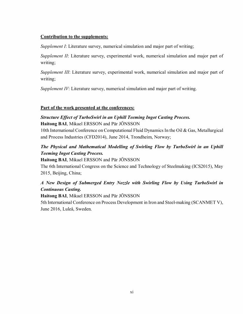
Contribution to the supplements:

Supplement I: Literature survey, numerical simulation and major part of writing;

Supplement II: Literature survey, experimental work, numerical simulation and major part of writing;

Supplement III: Literature survey, experimental work, numerical simulation and major part of writing;

Supplement IV: Literature survey, numerical simulation and major part of writing.

Part of the work presented at the conferences:

Structure Effect of TurboSwirl in an Uphill Teeming Ingot Casting Process. Haitong BAI, Mikael ERSSON and Pär JÖNSSON 10th International Conference on Computational Fluid Dynamics In the Oil & Gas, Metallurgical and Process Industries (CFD2014), June 2014, Trondheim, Norway;

The Physical and Mathematical Modelling of Swirling Flow by TurboSwirl in an Uphill Teeming Ingot Casting Process. Haitong BAI, Mikael ERSSON and Pär JÖNSSON The 6th International Congress on the Science and Technology of Steelmaking (ICS2015), May 2015, Beijing, China;

A New Design of Submerged Entry Nozzle with Swirling Flow by Using TurboSwirl in Continuous Casting. Haitong BAI, Mikael ERSSON and Pär JÖNSSON 5th International Conference on Process Development in Iron and Steel-making (SCANMET V), June 2016, Luleå, Sweden.

xii

Contents

Abstract ................................................................................................................................................ v

Sammanfattning ................................................................................................................................ vii

Acknowledgment ................................................................................................................................. ix

Preface ................................................................................................................................................. x

Chapter 1 Introduction ........................................................................................................................ 1

1.1 Research background ..................................................................................................................1

1.2 Benefits of using swirling flow ....................................................................................................3

1.3 Objectives and content of this thesis ............................................................................................5

Chapter 2 The Numerical Modeling .................................................................................................... 6

2.1 Model domains ...........................................................................................................................6

2.1.1 Domain of the optimization of the TurboSwirl structure (Supplement I) ................................6

2.1.2 Domain of the validation of the TurboSwirl structure (Supplement II) ...................................8

2.1.3 Domain of the new implementation of the reverse TurboSwirl with mold (Supplement III) ...9

2.1.4 Domain of the improvement of the divergent reverse TurboSwirl nozzle with mold (Supplement IV) .......................................................................................................................... 10

2.2 Assumptions ............................................................................................................................. 12

2.3 Turbulence models .................................................................................................................... 12

2.3.1 The standard k-ɛ turbulence model (Supplements I & II) ..................................................... 12

2.3.2 The realizable k-ɛ turbulence model (Supplements II & III) ................................................ 13

2.3.3 The Reynolds stress turbulence model (RSM) (Supplements II & III) .................................. 13

2.3.4 The detached eddy simulation turbulence model (DES) (Supplements III & IV) .................. 14

2.4 The volume of fluid (VOF) model (Supplement II) .................................................................... 15

2.5 Boundary conditions ................................................................................................................. 16

2.6 Simulation methods................................................................................................................... 16

Chapter 3 The Water Model Experiment ........................................................................................... 18

3.1 Water model for uphill teeming ................................................................................................. 18

3.2 Water model for reverse TurboSwirl and mold .......................................................................... 20

3.3 Ultrasonic velocity profiler (UVP)............................................................................................. 20

3.4 Velocity measurement by UVP for water model of uphill teeming ............................................. 21

xiii

3.5 Velocity measurement by UVP for water model of reverse TurboSwirl ..................................... 22

Chapter 4 Results and Discussion ..................................................................................................... 24

4.1 Optimization of the TurboSwirl structure for uphill teeming ..................................................... 24

4.1.1 Validation and mesh sensitivity .......................................................................................... 24

4.1.2 Optimization of the flaring angle ........................................................................................ 29

4.1.3 Optimization of the position of the vertical runner .............................................................. 32

4.2 Validation of predicted TurboSwirl for uphill teeming by water model experiments .................. 35

4.2.1 Comparison of turbulence models for numerical modelling ................................................ 35

4.2.2 Radial velocity measurement by UVP ................................................................................ 38

4.2.3 Vortex shape ...................................................................................................................... 40

4.3 New implementation of the reverse TurboSwirl in continuous casting process .......................... 42

4.3.1 Axial velocity validation .................................................................................................... 42

4.3.2 Tangential velocity validation ............................................................................................ 45

4.3.3. Time per cycle with different inlet velocities ..................................................................... 46

4.3.4. Comparison of swirling flow between the reverse TurboSwirl and the electromagnetic swirl flow generator ............................................................................................................................ 48

4.4 Improvement by the divergent reverse TurboSwirl nozzle (DRTSN) in the continuous casting process ........................................................................................................................................... 51

4.4.1 The comparison of the SRTSN and the DRTSN ................................................................. 51

4.4.2 The effect of the inlet velocity on the flow pattern .............................................................. 56

4.4.3 The effect of the length of the horizontal runner on the flow pattern ................................... 59

Chapter 5 Conclusion........................................................................................................................ 62

Chapter 6 Future Work ..................................................................................................................... 65

References ......................................................................................................................................... 66

xiv

1

Chapter 1 Introduction

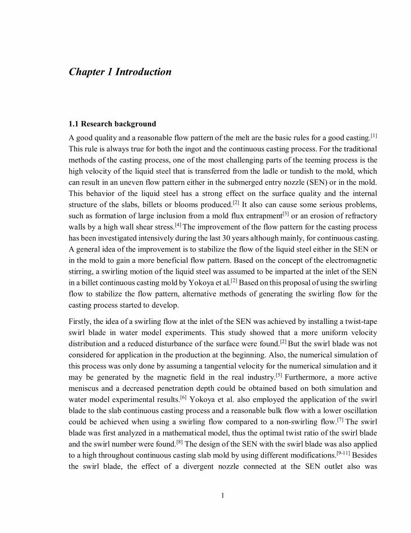
1.1 Research background

A good quality and a reasonable flow pattern of the melt are the basic rules for a good casting.[1] This rule is always true for both the ingot and the continuous casting process. For the traditional methods of the casting process, one of the most challenging parts of the teeming process is the high velocity of the liquid steel that is transferred from the ladle or tundish to the mold, which can result in an uneven flow pattern either in the submerged entry nozzle (SEN) or in the mold. This behavior of the liquid steel has a strong effect on the surface quality and the internal structure of the slabs, billets or blooms produced.[2] It also can cause some serious problems, such as formation of large inclusion from a mold flux entrapment[3] or an erosion of refractory walls by a high wall shear stress.[4] The improvement of the flow pattern for the casting process has been investigated intensively during the last 30 years although mainly, for continuous casting. A general idea of the improvement is to stabilize the flow of the liquid steel either in the SEN or in the mold to gain a more beneficial flow pattern. Based on the concept of the electromagnetic stirring, a swirling motion of the liquid steel was assumed to be imparted at the inlet of the SEN in a billet continuous casting mold by Yokoya et al.[2] Based on this proposal of using the swirling flow to stabilize the flow pattern, alternative methods of generating the swirling flow for the casting process started to develop.

Firstly, the idea of a swirling flow at the inlet of the SEN was achieved by installing a twist-tape swirl blade in water model experiments. This study showed that a more uniform velocity distribution and a reduced disturbance of the surface were found.[2] But the swirl blade was not considered for application in the production at the beginning. Also, the numerical simulation of this process was only done by assuming a tangential velocity for the numerical simulation and it may be generated by the magnetic field in the real industry.[5] Furthermore, a more active meniscus and a decreased penetration depth could be obtained based on both simulation and water model experimental results.[6] Yokoya et al. also employed the application of the swirl blade to the slab continuous casting process and a reasonable bulk flow with a lower oscillation could be achieved when using a swirling flow compared to a non-swirling flow.[7] The swirl blade was first analyzed in a mathematical model, thus the optimal twist ratio of the swirl blade and the swirl number were found.[8] The design of the SEN with the swirl blade was also applied to a high throughout continuous casting slab mold by using different modifications.[9-11] Besides the swirl blade, the effect of a divergent nozzle connected at the SEN outlet also was

2

considered.[2] The angle of the divergent nozzle was optimized based on the velocity and heat distribution in a billet mold.[12] The effect of the swirl blade also was studied by Solorio-Diaz et al.[13-16] for the swirling ladle shroud in the tundish. The results of water model and numerical simulation revealed that that the generated swirling flow can reduce the impact velocity and the turbulence of the entering jet compared with a conventional ladle shroud in the tundish.

However, a swirl blade is difficult to manufacture when it is inserted in the casting system. There is also a risk that the runner or SEN will be clogged with nonmetallic inclusions.[17] This is detrimental to the solidification of the liquid steel. In this case, some researchers have tried to use an additional device or to change the structure without inserting anything into the gating system to generate the swirling flow. One example is to use a centrifugal flow in the tundish.[18] Hou et al. used a swirl chamber inside the tundish to generate a swirling flow and they found that the swirling flow became asymmetric.[19-20] Ni et al. redesigned the tundish with a cylindrical part connected the SEN to generate a swirling flow and to study the maximum wall shear stresses and non-metallic inclusion behaviors.[21-22] The strength of the swirling flow was found to decrease when the liquid steel flowed into the SEN and the mold, so a rotating electromagnetic filed was placed around the immersion nozzle[23-25] or the mold[26] to induce the swirling flow. Also, a strong swirling flow can effectively reduce the downwards axial velocities and homogenize the temperature distribution in the mold.[27]

The swirling flow has also been investigated a lot for the uphill teeming ingot casting process. Although the steel products of the ingot casting process account for much smaller than that produced by the continuous casting process, some special steel, such as forgings and low-alloyed steel can only be produced by the ingot casting process.[28] With respect to the teeming mode, the bottom teeming is more widely used, since it can reduce the turbulence significantly compared to using a top teeming technique during the pouring process.[29] The liquid steel will flow uphill from the runner to the bottom of the mold. For the traditional filling of the mold, the complex inclusion composition in the mold could be found due to the reaction between the mold flux and the liquid steel.[30] The inlet angle of the mold was increased to decrease the disturbance of the free surface, which resulted in less mold flux entrapments.[31] The initial filling height and maximum wall shear stress were then studied by Tan et al. by using both full and reduced geometry models.[32] However, unevennesses of the flow field still can still be found when using an increased inlet angle of the mold. Hallgren et al. studied the swirl blade inserted into the vertical runner below the ingot mold with a divergent nozzle to reduce the unevenness based on both numerical simulations and the water model experiments.[33-34] It was found that the initial filling could form a more stable flow pattern with these improvement of the swirling flow.[35] The vertical position[36] and the orientation[37] of the swirl blade in the runner were also investigated. The plant trials were carried out to further study the availability of utilizing the

3

swirl blade with a calmer filling condition[36] and a more even lubrication by the mold flux[38] in the mold.

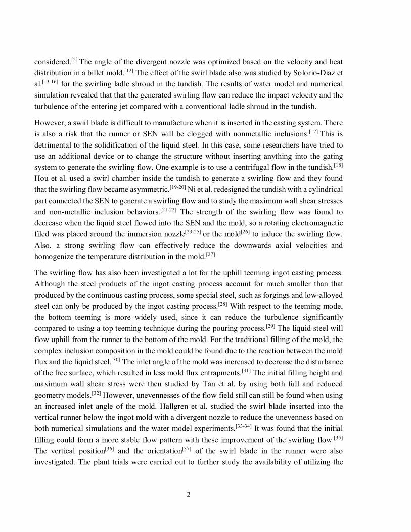
Fig. 1.1. The sketch of the TurboSwirl device.

As discussed above, the swirl blade has some limitations, for example, there is an increased risk that clogging may occur. However, the electromagnetic stirring usually has a high energy consumption. On the basis of the previous studies of the swirling flow pattern, a new swirling flow generator, the TurboSwirl device, was introduced for the ingot casting process of steel.[39]

A typical sketch of the TurboSwirl device is shown in Figure 1.1. The original concept of this geometry setup can be traced back to a patent in 1914.[40] A similar design of changing the geometry was used to generate a swirling flow for filtration[41] and aluminum gravity casting.[42]

The TurboSwirl device is located at the intersection of the horizontal and vertical runners below the mold. The liquid steel enters the large cylinder from the horizontal runner, and creates a swirling flow motion before leaving through the vertical runner. A divergent nozzle can be used after the vertical runner to further improve the setup. This device was first modelled by Tan et al. in the ingot casting process of steel.[39] During the initial filling condition, the flow pattern could be improved a lot by the TurboSwirl implementation. For example, a much calmer filling condition and lower hump height could be found compared to when using the swirl blade and a decreased maximum wall shear stress with fewer fluctuations. In addition, the removal of non-metallic inclusion was also enhanced by the use of the TurboSwirl device.[43]

1.2 Benefits of using swirling flow

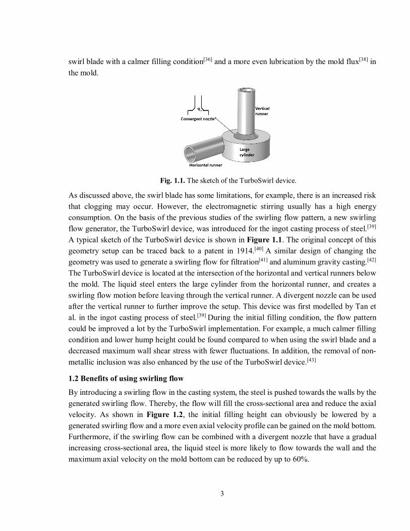
By introducing a swirling flow in the casting system, the steel is pushed towards the walls by the generated swirling flow. Thereby, the flow will fill the cross-sectional area and reduce the axial velocity. As shown in Figure 1.2, the initial filling height can obviously be lowered by a generated swirling flow and a more even axial velocity profile can be gained on the mold bottom. Furthermore, if the swirling flow can be combined with a divergent nozzle that have a gradual increasing cross-sectional area, the liquid steel is more likely to flow towards the wall and the maximum axial velocity on the mold bottom can be reduced by up to 60%.

4

Fig. 1.2. The predicted liquid volume fraction on the central cross-section and the axial velocity profile on the mold bottom of the molten steel for initial uphill filling (a) without a swirling flow, (b) with a

generated swirling flow and (c) with a generated swirling flow and a divergent nozzle.

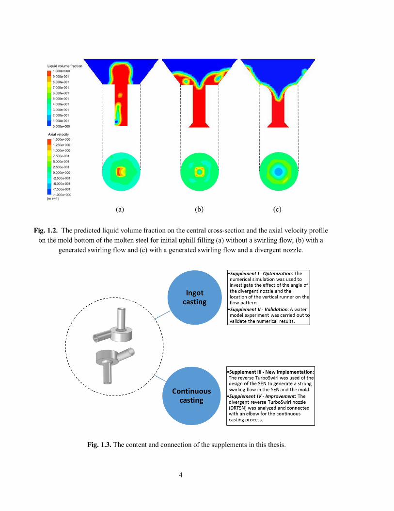
Fig. 1.3. The content and connection of the supplements in this thesis.

5

1.3 Objectives and content of this thesis

In this thesis, the swirling flow pattern generated by the TurboSwirl device in the casting process was further studied by numerical simulations and water model experiments. Four supplement papers are included in this thesis. The content and the connection of these supplements are shown in Figure 1.3. As discussed above, the utilizing of the TurboSwirl in the ingot casting process could result in calmer filling conditions and lower hump heights, but higher wall shear stresses were also found in the region of the convergent nozzle.[39] Therefore, the first objective of this thesis work was to optimize the structure of the TurboSwirl by numerical simulations to achieve a lower maximum wall shear stress and a lower maximum axial velocity while maintaining a strong enough swirling flow in the ingot casting process of steel. This is discussed (Supplement I). Secondly, the mathematical model of the optimized TurboSwirl was validated by water model experiments based on measurement of the ultrasonic velocity profiler (UVP) setup (Supplement II). Furthermore, the idea of generating the swirling flow by the TurboSwirl was implemented to the design of the submerged entry nozzle (SEN) in the continuous casting process of steel based on both mathematical and physical models (Supplement III). At last, the new design was improved by the introduction of the divergent reverse TurboSwirl nozzle (DRTSN), and the method of the connection between the TurboSwirl and ladle was proposed and studied to obtain a more beneficial swirling flow pattern (Supplement IV).

6

Chapter 2 The Numerical Modeling

During the development of the metallurgical processes of the last few decades, the research work have been improved significantly by the use of computational fluid dynamics (CFD).[44-45] The numerical results can help the steel producers to improve and redesign the metallurgical process to raise the productivity and to decrease the costs.[46] The study of the swirling flow has also been intensively investigated by using numerical simulations. Therefore, the work in this thesis also used CFD simulations as the main method to investigate the swirling flow pattern by introducing the TurboSwirl device into casting processes.

2.1 Model domains

2.1.1 Domain of the optimization of the TurboSwirl structure (Supplement I)

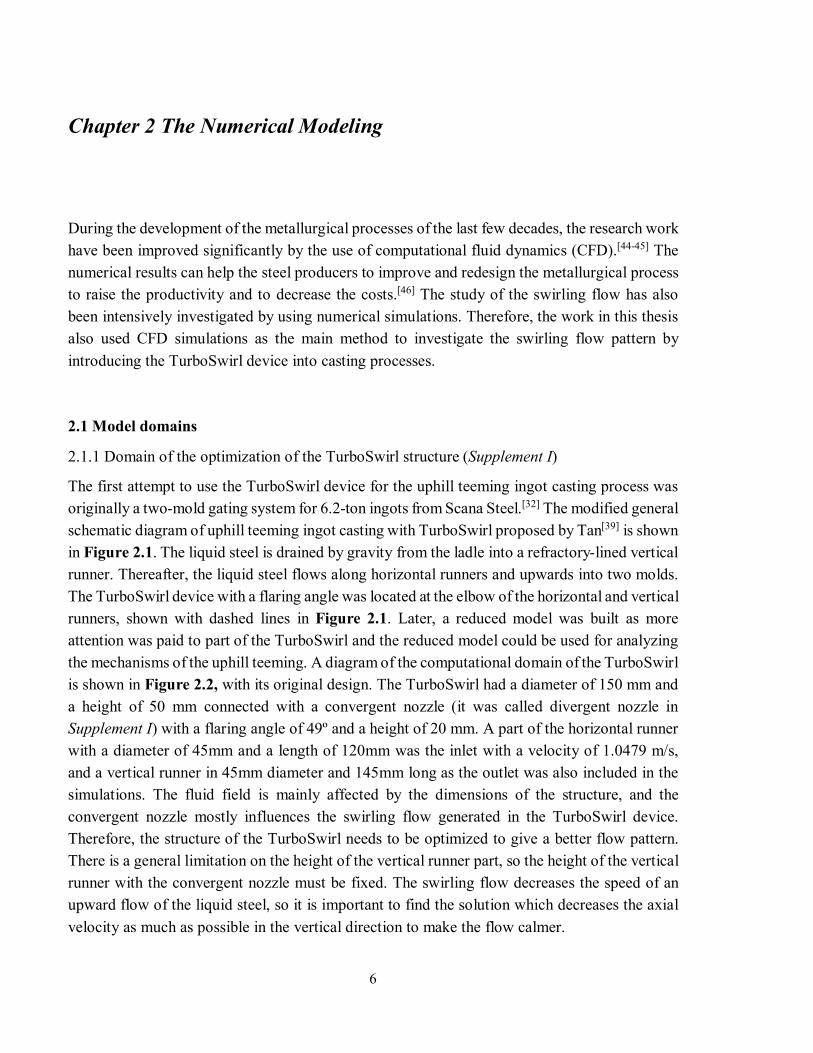
The first attempt to use the TurboSwirl device for the uphill teeming ingot casting process was originally a two-mold gating system for 6.2-ton ingots from Scana Steel.[32] The modified general schematic diagram of uphill teeming ingot casting with TurboSwirl proposed by Tan[39] is shown in Figure 2.1. The liquid steel is drained by gravity from the ladle into a refractory-lined vertical runner. Thereafter, the liquid steel flows along horizontal runners and upwards into two molds. The TurboSwirl device with a flaring angle was located at the elbow of the horizontal and vertical runners, shown with dashed lines in Figure 2.1. Later, a reduced model was built as more attention was paid to part of the TurboSwirl and the reduced model could be used for analyzing the mechanisms of the uphill teeming. A diagram of the computational domain of the TurboSwirl is shown in Figure 2.2, with its original design. The TurboSwirl had a diameter of 150 mm and a height of 50 mm connected with a convergent nozzle (it was called divergent nozzle in Supplement I) with a flaring angle of 49º and a height of 20 mm. A part of the horizontal runner with a diameter of 45mm and a length of 120mm was the inlet with a velocity of 1.0479 m/s, and a vertical runner in 45mm diameter and 145mm long as the outlet was also included in the simulations. The fluid field is mainly affected by the dimensions of the structure, and the convergent nozzle mostly influences the swirling flow generated in the TurboSwirl device. Therefore, the structure of the TurboSwirl needs to be optimized to give a better flow pattern. There is a general limitation on the height of the vertical runner part, so the height of the vertical runner with the convergent nozzle must be fixed. The swirling flow decreases the speed of an upward flow of the liquid steel, so it is important to find the solution which decreases the axial velocity as much as possible in the vertical direction to make the flow calmer.

7

Fig. 2.1. Schematic diagram of ingot casting (unit: mm)[39].

Fig. 2.2. Dimensions of computational domain of the TurboSwirl device (original design, unit: mm).

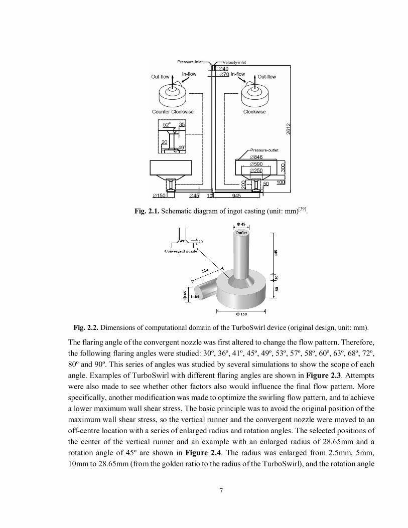
The flaring angle of the convergent nozzle was first altered to change the flow pattern. Therefore, the following flaring angles were studied: 30º, 36º, 41º, 45º, 49º, 53º, 57º, 58º, 60º, 63º, 68º, 72º, 80º and 90º. This series of angles was studied by several simulations to show the scope of each angle. Examples of TurboSwirl with different flaring angles are shown in Figure 2.3. Attempts were also made to see whether other factors also would influence the final flow pattern. More specifically, another modification was made to optimize the swirling flow pattern, and to achieve a lower maximum wall shear stress. The basic principle was to avoid the original position of the maximum wall shear stress, so the vertical runner and the convergent nozzle were moved to an off-centre location with a series of enlarged radius and rotation angles. The selected positions of the center of the vertical runner and an example with an enlarged radius of 28.65mm and a rotation angle of 45º are shown in Figure 2.4. The radius was enlarged from 2.5mm, 5mm, 10mm to 28.65mm (from the golden ratio to the radius of the TurboSwirl), and the rotation angle

8

α was changed from 90º to -90º based on the cross section of the TurboSwirl. Also, Zone I (0º<α<90º) and Zone II (-90º<α<0º) were separated to indicate the approximate area of modification. The flaring angle of the convergent nozzle was kept at 49º for the original design to facilitate a comparison of the results and to determine whether there was any improvements as a result of these modifications.

Fig. 2.3. Examples of different flaring angles: (a): 30º; (b): 60º; (c): 90º.

Fig. 2.4. (a): Selected position (black points indicate the center of vertical runner, 25 points in all, unit: mm) with an enlarged radius (from 2.5mm, 5mm, 10mm to 28.65mm) and different rotation angles

(from 90º, 45º, 0º, -45º to -90º) for off-centre calculation (unit: mm); (b): Computational domain for the center of the vertical runner on black point A with an enlarged radius of 28.65mm and a rotation angle

of 45º.

2.1.2 Domain of the validation of the TurboSwirl structure (Supplement II)

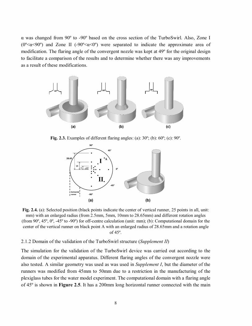
The simulation for the validation of the TurboSwirl device was carried out according to the domain of the experimental apparatus. Different flaring angles of the convergent nozzle were also tested. A similar geometry was used as was used in Supplement I, but the diameter of the runners was modified from 45mm to 50mm due to a restriction in the manufacturing of the plexiglass tubes for the water model experiment. The computational domain with a flaring angle of 45º is shown in Figure 2.5. It has a 200mm long horizontal runner connected with the main

9

part of the TurboSwirl, which is a large cylinder with a diameter of 150mm. The inlet was located on the horizontal runner. A constant velocity of 0.36m/s calculated from the experimental flow rate was applied as a velocity condition at the inlet. A convergent nozzle is placed above the large cylinder with a flaring angle α, which connects the larger cylinder and the vertical runner. Considering the difficulty of manufacturing the experimental devices, five groups of flaring angles were chosen based on the results from the study in Supplement I: 26.5º, 32º, 45º, 59º and 68º.

Fig. 2.5. The computational domain according to the experimental apparatus with flaring angle of 45º (unit: mm).

2.1.3 Domain of the new implementation of the reverse TurboSwirl with mold (Supplement III)

The TurboSwirl device was reversed and applied to the billet continuous casting process. A three-dimensional mathematical model of the reverse TurboSwirl and a round billet mold was built. The dimension of the computational domain is shown in Figure 2.6. The fluid flows into the horizontal runner of the reverse TurboSwirl and flows out from the vertical runner to the mold. The inlet was placed on the horizontal runner and the steel had a constant velocity, which was calculated from the experimental flow rate. Specifically, a value of 0.75 m/s was applied as a velocity condition at the inlet. The submerged depth was 120 mm from the meniscus to the outlet of the SEN. The mold has a diameter of 635 mm and a height of 670 mm. Also, there is a small outlet on the bottom of the mold to simulate the pump used in the water model experiment.

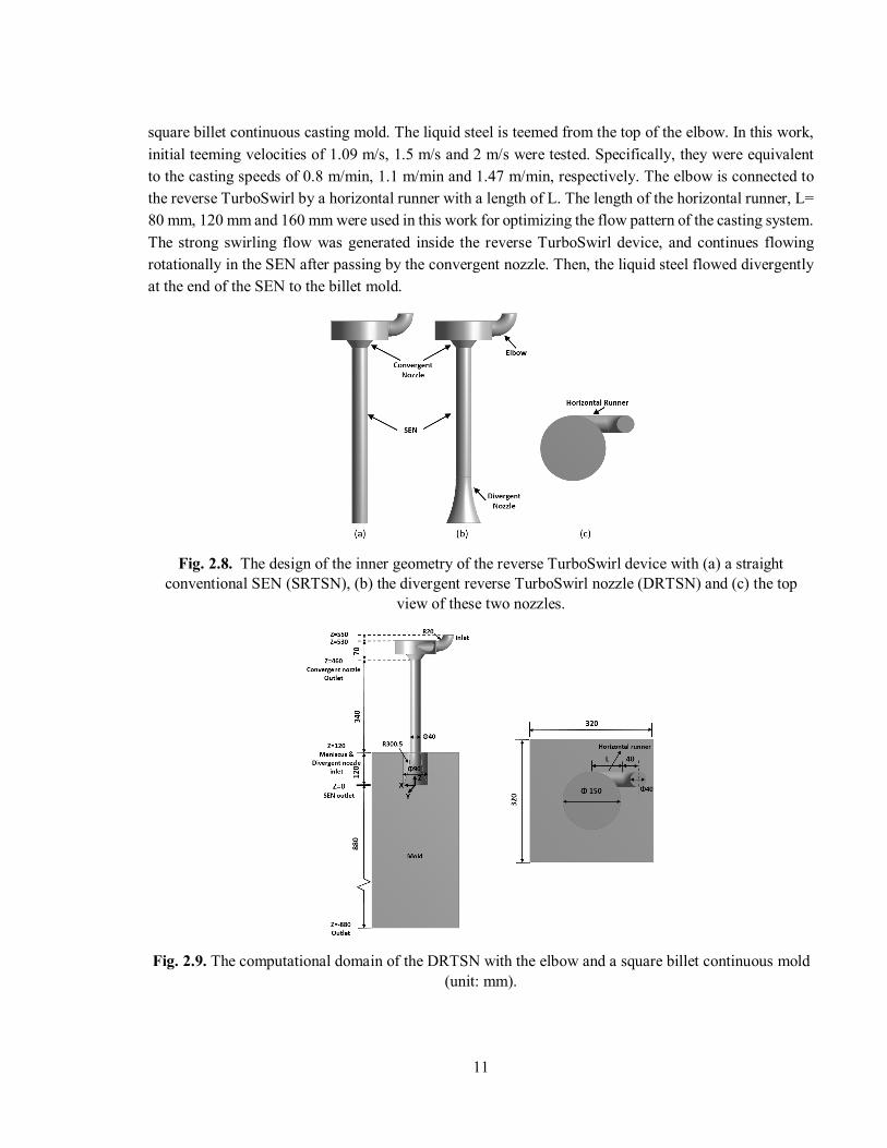
The design of the TurboSwirl for the SEN was further applied to a square billet continuous casting process, which originally used an electromagnetic swirl flow generator (EMSFG) to generate a swirling flow around the center of the SEN.[27] The dimension and sketch of the square billet continuous casting setup, including the square mold and the SEN connected with the reverse TurboSwirl, are shown in Figure 2.7. The reverse TurboSwirl device is placed on the top of the SEN. It has a total height of 70 mm and the straight SEN part is 480 mm, while the total height of the SEN was kept the same as in the original SEN.[27] In order to generate the swirling flow inside the TurboSwirl, the same inlet condition was used. The inlet velocity was

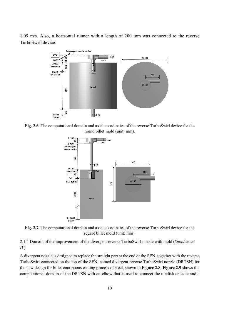
10

1.09 m/s. Also, a horizontal runner with a length of 200 mm was connected to the reverse TurboSwirl device.

Fig. 2.6. The computational domain and axial coordinates of the reverse TurboSwirl device for the round billet mold (unit: mm).

Fig. 2.7. The computational domain and axial coordinates of the reverse TurboSwirl device for the square billet mold (unit: mm).

2.1.4 Domain of the improvement of the divergent reverse TurboSwirl nozzle with mold (Supplement IV)

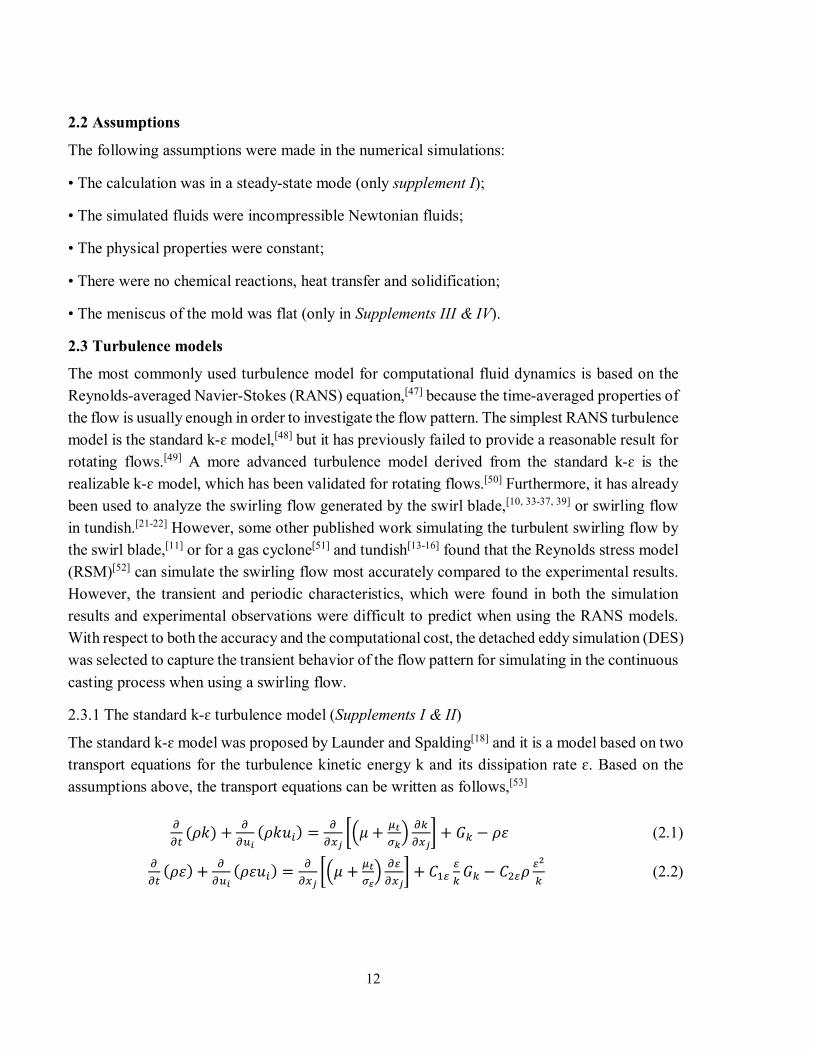
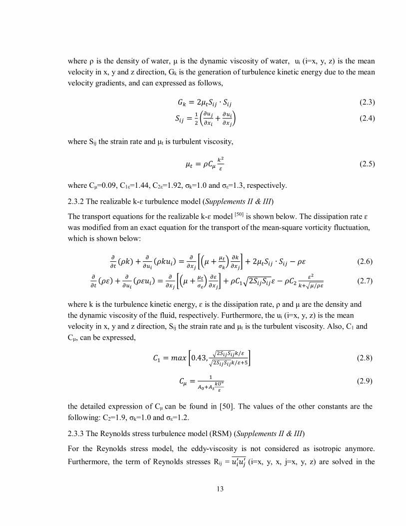
A divergent nozzle is designed to replace the straight part at the end of the SEN, together with the reverse TurboSwirl connected on the top of the SEN, named divergent reverse TurboSwirl nozzle (DRTSN) for the new design for billet continuous casting process of steel, shown in Figure 2.8. Figure 2.9 shows the computational domain of the DRTSN with an elbow that is used to connect the tundish or ladle and a

11

square billet continuous casting mold. The liquid steel is teemed from the top of the elbow. In this work, initial teeming velocities of 1.09 m/s, 1.5 m/s and 2 m/s were tested. Specifically, they were equivalent to the casting speeds of 0.8 m/min, 1.1 m/min and 1.47 m/min, respectively. The elbow is connected to the reverse TurboSwirl by a horizontal runner with a length of L. The length of the horizontal runner, L= 80 mm, 120 mm and 160 mm were used in this work for optimizing the flow pattern of the casting system. The strong swirling flow was generated inside the reverse TurboSwirl device, and continues flowing rotationally in the SEN after passing by the convergent nozzle. Then, the liquid steel flowed divergently at the end of the SEN to the billet mold.

Fig. 2.8. The design of the inner geometry of the reverse TurboSwirl device with (a) a straight conventional SEN (SRTSN), (b) the divergent reverse TurboSwirl nozzle (DRTSN) and (c) the top

view of these two nozzles.

Fig. 2.9. The computational domain of the DRTSN with the elbow and a square billet continuous mold (unit: mm).

12

2.2 Assumptions

The following assumptions were made in the numerical simulations:

• The calculation was in a steady-state mode (only supplement I);

• The simulated fluids were incompressible Newtonian fluids;

• The physical properties were constant;

• There were no chemical reactions, heat transfer and solidification;

• The meniscus of the mold was flat (only in Supplements III & IV).

2.3 Turbulence models

The most commonly used turbulence model for computational fluid dynamics is based on the Reynolds-averaged Navier-Stokes (RANS) equation,[47] because the time-averaged properties of the flow is usually enough in order to investigate the flow pattern. The simplest RANS turbulence model is the standard k-ɛ model,[48] but it has previously failed to provide a reasonable result for rotating flows.[49] A more advanced turbulence model derived from the standard k-ɛ is the realizable k-ɛ model, which has been validated for rotating flows.[50] Furthermore, it has already been used to analyze the swirling flow generated by the swirl blade,[10, 33-37, 39] or swirling flow in tundish.[21-22] However, some other published work simulating the turbulent swirling flow by the swirl blade,[11] or for a gas cyclone[51] and tundish[13-16] found that the Reynolds stress model (RSM)[52] can simulate the swirling flow most accurately compared to the experimental results. However, the transient and periodic characteristics, which were found in both the simulation results and experimental observations were difficult to predict when using the RANS models. With respect to both the accuracy and the computational cost, the detached eddy simulation (DES) was selected to capture the transient behavior of the flow pattern for simulating in the continuous casting process when using a swirling flow.

2.3.1 The standard k-ɛ turbulence model (Supplements I & II)

The standard k-ɛ model was proposed by Launder and Spalding[18] and it is a model based on two transport equations for the turbulence kinetic energy k and its dissipation rate ɛ. Based on the assumptions above, the transport equations can be written as follows,[53]

( ) + ( ) = + + − (2.1)

( ) + ( ) = + + − (2.2)

13

where ρ is the density of water, μ is the dynamic viscosity of water, ui (i=x, y, z) is the mean velocity in x, y and z direction, Gk is the generation of turbulence kinetic energy due to the mean velocity gradients, and can expressed as follows,

= 2 ∙ (2.3)

= + (2.4)

where Sij the strain rate and μt is turbulent viscosity,

= (2.5)

where Cμ=0.09, C1ε=1.44, C2ε=1.92, σk=1.0 and σε=1.3, respectively.

2.3.2 The realizable k-ɛ turbulence model (Supplements II & III)

The transport equations for the realizable k-ɛ model [50] is shown below. The dissipation rate ɛ was modified from an exact equation for the transport of the mean-square vorticity fluctuation, which is shown below:

( ) + ( ) = + + 2 ∙ − (2.6)

( ) + ( ) = + + 2 −/

(2.7)

where k is the turbulence kinetic energy, ɛ is the dissipation rate, ρ and μ are the density and the dynamic viscosity of the fluid, respectively. Furthermore, the ui (i=x, y, z) is the mean velocity in x, y and z direction, Sij the strain rate and μt is the turbulent viscosity. Also, C1 and Cμ, can be expressed,

= 0.43,/

/ (2.8)

= ∗ (2.9)

the detailed expression of Cμ can be found in [50]. The values of the other constants are the following: C2=1.9, σk=1.0 and σε=1.2.

2.3.3 The Reynolds stress turbulence model (RSM) (Supplements II & III)

For the Reynolds stress model, the eddy-viscosity is not considered as isotropic anymore. Furthermore, the term of Reynolds stresses Rij = (i=x, y, x, j=x, y, z) are solved in the

14

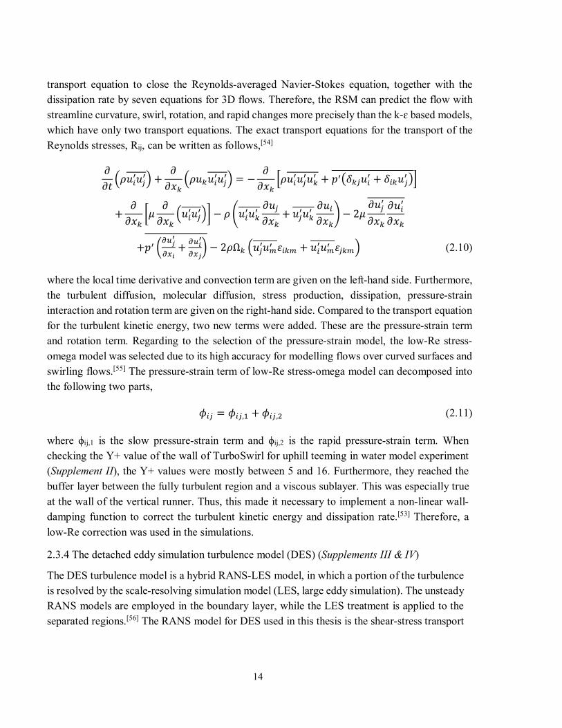
transport equation to close the Reynolds-averaged Navier-Stokes equation, together with the dissipation rate by seven equations for 3D flows. Therefore, the RSM can predict the flow with streamline curvature, swirl, rotation, and rapid changes more precisely than the k-ɛ based models, which have only two transport equations. The exact transport equations for the transport of the Reynolds stresses, Rij, can be written as follows,[54]

+ = − + +

+ − + − 2

+ + − 2 Ω + (2.10)

where the local time derivative and convection term are given on the left-hand side. Furthermore, the turbulent diffusion, molecular diffusion, stress production, dissipation, pressure-strain interaction and rotation term are given on the right-hand side. Compared to the transport equation for the turbulent kinetic energy, two new terms were added. These are the pressure-strain term and rotation term. Regarding to the selection of the pressure-strain model, the low-Re stress-omega model was selected due to its high accuracy for modelling flows over curved surfaces and swirling flows.[55] The pressure-strain term of low-Re stress-omega model can decomposed into the following two parts,

= , + , (2.11)

where ϕij,1 is the slow pressure-strain term and ϕij,2 is the rapid pressure-strain term. When checking the Y+ value of the wall of TurboSwirl for uphill teeming in water model experiment (Supplement II), the Y+ values were mostly between 5 and 16. Furthermore, they reached the buffer layer between the fully turbulent region and a viscous sublayer. This was especially true at the wall of the vertical runner. Thus, this made it necessary to implement a non-linear wall-damping function to correct the turbulent kinetic energy and dissipation rate.[53] Therefore, a low-Re correction was used in the simulations.

2.3.4 The detached eddy simulation turbulence model (DES) (Supplements III & IV)

The DES turbulence model is a hybrid RANS-LES model, in which a portion of the turbulence is resolved by the scale-resolving simulation model (LES, large eddy simulation). The unsteady RANS models are employed in the boundary layer, while the LES treatment is applied to the separated regions.[56] The RANS model for DES used in this thesis is the shear-stress transport

15

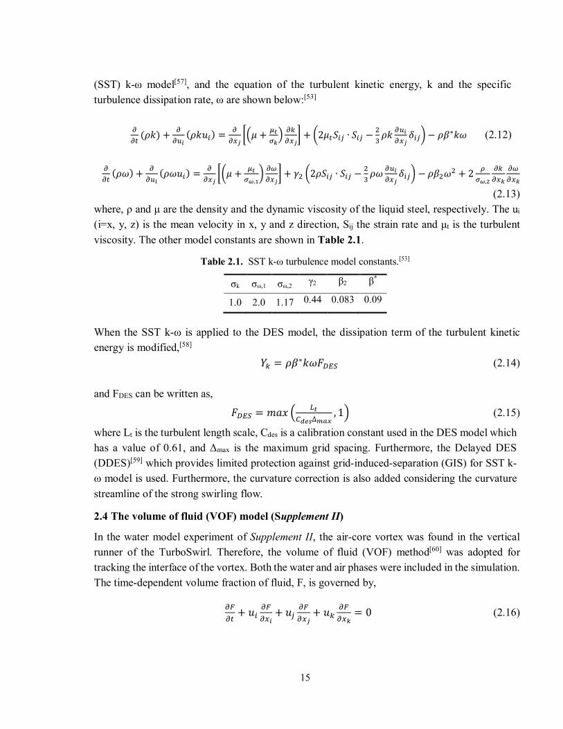
(SST) k-ω model[57], and the equation of the turbulent kinetic energy, k and the specific turbulence dissipation rate, ω are shown below:[53]

( ) + ( ) = + + 2 ∙ − − ∗ (2.12)

( ) + ( ) = +,

+ 2 ∙ − − + 2,

(2.13) where, ρ and μ are the density and the dynamic viscosity of the liquid steel, respectively. The ui (i=x, y, z) is the mean velocity in x, y and z direction, Sij the strain rate and μt is the turbulent viscosity. The other model constants are shown in Table 2.1.

Table 2.1. SST k-ω turbulence model constants.[53]

σk σω,1 σω,2 γ2 β2 β*

1.0 2.0 1.17 0.44 0.083 0.09

When the SST k-ω is applied to the DES model, the dissipation term of the turbulent kinetic energy is modified,[58]

= ∗ (2.14) and FDES can be written as,

=∆

, 1 (2.15)

where Lt is the turbulent length scale, Cdes is a calibration constant used in the DES model which has a value of 0.61, and Δmax is the maximum grid spacing. Furthermore, the Delayed DES (DDES)[59] which provides limited protection against grid-induced-separation (GIS) for SST k-ω model is used. Furthermore, the curvature correction is also added considering the curvature streamline of the strong swirling flow.

2.4 The volume of fluid (VOF) model (Supplement II)

In the water model experiment of Supplement II, the air-core vortex was found in the vertical runner of the TurboSwirl. Therefore, the volume of fluid (VOF) method[60] was adopted for tracking the interface of the vortex. Both the water and air phases were included in the simulation. The time-dependent volume fraction of fluid, F, is governed by,

+ + + = 0 (2.16)

16

2.5 Boundary conditions

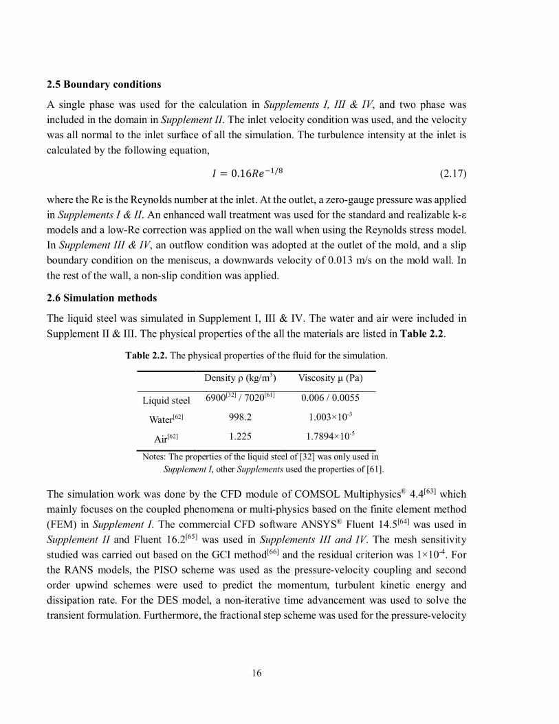
A single phase was used for the calculation in Supplements I, III & IV, and two phase was included in the domain in Supplement II. The inlet velocity condition was used, and the velocity was all normal to the inlet surface of all the simulation. The turbulence intensity at the inlet is calculated by the following equation,

= 0.16 / (2.17)

where the Re is the Reynolds number at the inlet. At the outlet, a zero-gauge pressure was applied in Supplements I & II. An enhanced wall treatment was used for the standard and realizable k-ε models and a low-Re correction was applied on the wall when using the Reynolds stress model. In Supplement III & IV, an outflow condition was adopted at the outlet of the mold, and a slip boundary condition on the meniscus, a downwards velocity of 0.013 m/s on the mold wall. In the rest of the wall, a non-slip condition was applied.

2.6 Simulation methods

The liquid steel was simulated in Supplement I, III & IV. The water and air were included in Supplement II & III. The physical properties of the all the materials are listed in Table 2.2.

Table 2.2. The physical properties of the fluid for the simulation.

Density ρ (kg/m3) Viscosity μ (Pa)

Liquid steel 6900[32] / 7020[61] 0.006 / 0.0055

Water[62] 998.2 1.003×10-3

Air[62] 1.225 1.7894×10-5

Notes: The properties of the liquid steel of [32] was only used in Supplement I, other Supplements used the properties of [61].

The simulation work was done by the CFD module of COMSOL Multiphysics® 4.4[63] which mainly focuses on the coupled phenomena or multi-physics based on the finite element method (FEM) in Supplement I. The commercial CFD software ANSYS® Fluent 14.5[64] was used in Supplement II and Fluent 16.2[65] was used in Supplements III and IV. The mesh sensitivity studied was carried out based on the GCI method[66] and the residual criterion was 1×10-4. For the RANS models, the PISO scheme was used as the pressure-velocity coupling and second order upwind schemes were used to predict the momentum, turbulent kinetic energy and dissipation rate. For the DES model, a non-iterative time advancement was used to solve the transient formulation. Furthermore, the fractional step scheme was used for the pressure-velocity

17

coupling, a bounded central differencing was used for momentum, and second order upwind schemes were used for the turbulent kinetic energy and dissipation rate.

18

Chapter 3 The Water Model Experiment

Due to the similar kinematic viscosity of water in room temperature and liquid steel in 1600 °C, water model experiments always represent a cheap alternative compared to plant trials in order to investigate the flow pattern of liquid steel in the casting process. Besides, the water model experiments are easy to operate, accurate to carry out measurements in and they can be used as a validation of the mathematical model. The investigation of the swirling flow was also widely done with the help the water model experiments.[2, 5-15, 33-34] In this thesis, water models were setup to validate the mathematical model used in the numerical simulations.

3.1 Water model for uphill teeming

In Supplement II, the water model experiment was setup to only include the TurboSwirl device with different flaring angles. In total, five TurboSwirl devices were manufactured. The dimension of the TurboSwirl used in this experiment was taken from Tan,[39] but the diameter of the runners was modified from 45mm to 50mm due to a restriction in the manufacturing of the plexiglass tubes. Also, the convergent nozzle was placed above the large cylinder with a flaring angle α. Considering the difficulty of manufacturing the experimental devices, five groups of flaring angles were chosen according to results from the former study: 26.5º, 32º, 45º, 59º and 68º.

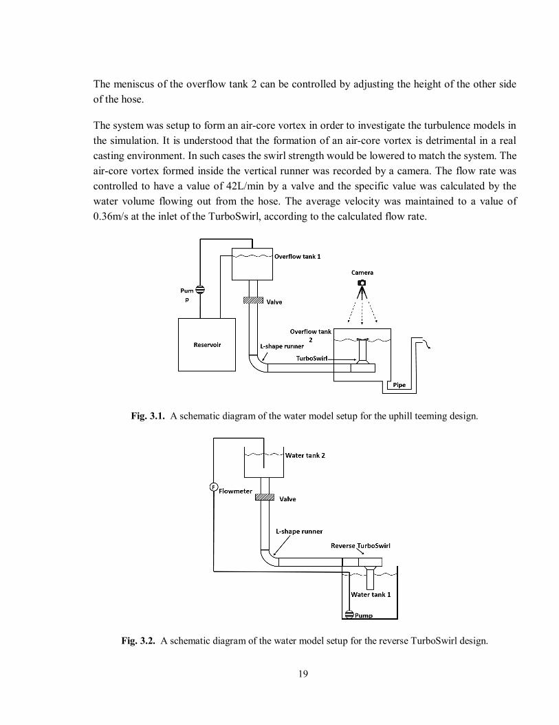
The whole water model experiment sketch is presented in Figure 3.1. The water was pumped from the reservoir to an overflow tank (Overflow tank 1). In addition, there was an outlet on the side of this overflow tank to supply a constant pressure to the whole system, so a constant velocity was obtained in the experiment. The water continued to flow to the long vertical pipe and the flow rate was controlled by a valve. Afterwards, the water flowed through a long horizontal pipe before flowing into the TurboSwirl device to make sure that an even velocity profile was obtained at the inlet of the TurboSwirl. The TurboSwirl was immersed into an overflow tank (Overflow tank 2), which is a transparent square plexiglass container that was used to eliminate the boundary curvature effect when using a camera to record the swirling flow and air-core vortex inside the TurboSwirl device.[67] In order to investigate the swirling flow of the TurboSwirl, a steady-state condition should be gained inside the vertical runner, so the mold, which was supposed to be placed on top of the TurboSwirl, was not included in this water model experiment. Furthermore, if an excessive amount of water submerged the outlet of the TurboSwirl, the pressure and velocity profile were not compatible with the reality, so the pressure gauge of the outlet of the TurboSwirl was kept at a zero value. Also, a long hose was connected to the bottom of the overflow tank 2.

19

The meniscus of the overflow tank 2 can be controlled by adjusting the height of the other side of the hose.

The system was setup to form an air-core vortex in order to investigate the turbulence models in the simulation. It is understood that the formation of an air-core vortex is detrimental in a real casting environment. In such cases the swirl strength would be lowered to match the system. The air-core vortex formed inside the vertical runner was recorded by a camera. The flow rate was controlled to have a value of 42L/min by a valve and the specific value was calculated by the water volume flowing out from the hose. The average velocity was maintained to a value of 0.36m/s at the inlet of the TurboSwirl, according to the calculated flow rate.

Fig. 3.1. A schematic diagram of the water model setup for the uphill teeming design.

Fig. 3.2. A schematic diagram of the water model setup for the reverse TurboSwirl design.

20

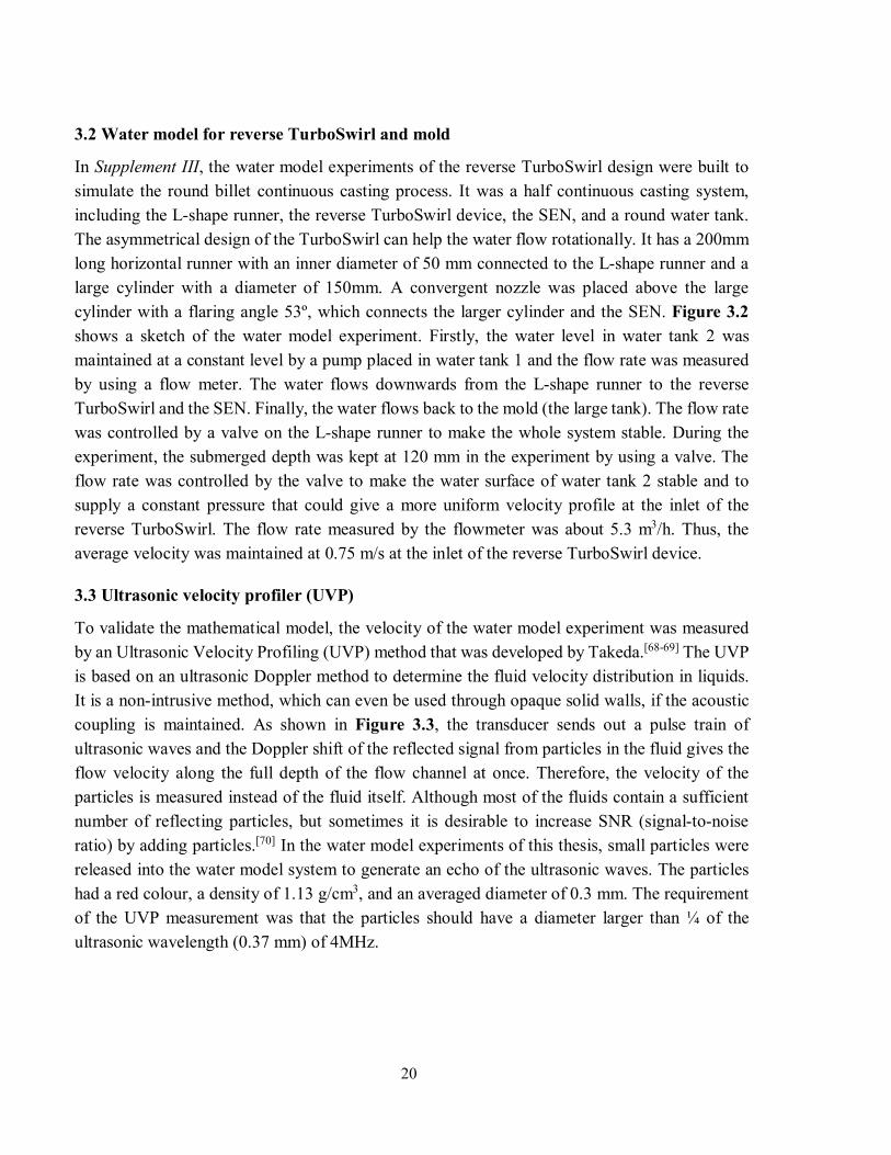
3.2 Water model for reverse TurboSwirl and mold

In Supplement III, the water model experiments of the reverse TurboSwirl design were built to simulate the round billet continuous casting process. It was a half continuous casting system, including the L-shape runner, the reverse TurboSwirl device, the SEN, and a round water tank. The asymmetrical design of the TurboSwirl can help the water flow rotationally. It has a 200mm long horizontal runner with an inner diameter of 50 mm connected to the L-shape runner and a large cylinder with a diameter of 150mm. A convergent nozzle was placed above the large cylinder with a flaring angle 53º, which connects the larger cylinder and the SEN. Figure 3.2 shows a sketch of the water model experiment. Firstly, the water level in water tank 2 was maintained at a constant level by a pump placed in water tank 1 and the flow rate was measured by using a flow meter. The water flows downwards from the L-shape runner to the reverse TurboSwirl and the SEN. Finally, the water flows back to the mold (the large tank). The flow rate was controlled by a valve on the L-shape runner to make the whole system stable. During the experiment, the submerged depth was kept at 120 mm in the experiment by using a valve. The flow rate was controlled by the valve to make the water surface of water tank 2 stable and to supply a constant pressure that could give a more uniform velocity profile at the inlet of the reverse TurboSwirl. The flow rate measured by the flowmeter was about 5.3 m3/h. Thus, the average velocity was maintained at 0.75 m/s at the inlet of the reverse TurboSwirl device.

3.3 Ultrasonic velocity profiler (UVP)

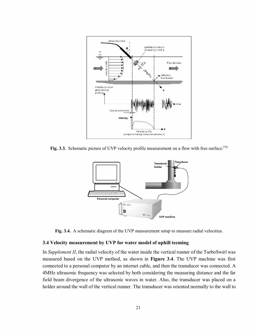
To validate the mathematical model, the velocity of the water model experiment was measured by an Ultrasonic Velocity Profiling (UVP) method that was developed by Takeda.[68-69] The UVP is based on an ultrasonic Doppler method to determine the fluid velocity distribution in liquids. It is a non-intrusive method, which can even be used through opaque solid walls, if the acoustic coupling is maintained. As shown in Figure 3.3, the transducer sends out a pulse train of ultrasonic waves and the Doppler shift of the reflected signal from particles in the fluid gives the flow velocity along the full depth of the flow channel at once. Therefore, the velocity of the particles is measured instead of the fluid itself. Although most of the fluids contain a sufficient number of reflecting particles, but sometimes it is desirable to increase SNR (signal-to-noise ratio) by adding particles.[70] In the water model experiments of this thesis, small particles were released into the water model system to generate an echo of the ultrasonic waves. The particles had a red colour, a density of 1.13 g/cm3, and an averaged diameter of 0.3 mm. The requirement of the UVP measurement was that the particles should have a diameter larger than ¼ of the ultrasonic wavelength (0.37 mm) of 4MHz.

21

Fig. 3.3. Schematic picture of UVP velocity profile measurement on a flow with free surface.[70]

Fig. 3.4. A schematic diagram of the UVP measurement setup to measure radial velocities.

3.4 Velocity measurement by UVP for water model of uphill teeming

In Supplement II, the radial velocity of the water inside the vertical runner of the TurboSwirl was measured based on the UVP method, as shown in Figure 3.4. The UVP machine was first connected to a personal computer by an internet cable, and then the transducer was connected. A 4MHz ultrasonic frequency was selected by both considering the measuring distance and the far field beam divergence of the ultrasonic waves in water. Also, the transducer was placed on a holder around the wall of the vertical runner. The transducer was oriented normally to the wall to

22

eliminate the refraction of the ultrasonic beam. Four positions along the height of the vertical runner were selected to measure the radial velocity. The heights were 99 mm, 119 mm, 139 mm and 159 mm. These were measured from the bottom of the TurboSwirl device to the vertical center of the transducer, where the ultrasonic beam was emitted.

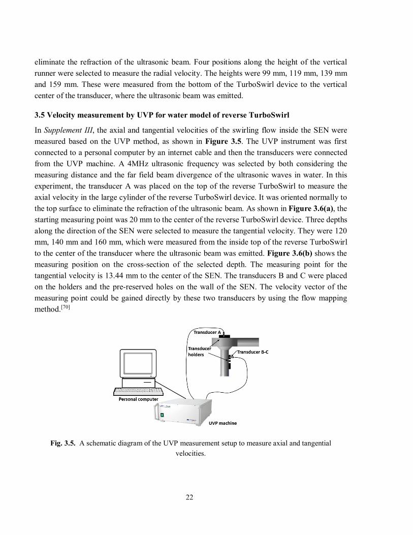
3.5 Velocity measurement by UVP for water model of reverse TurboSwirl

In Supplement III, the axial and tangential velocities of the swirling flow inside the SEN were measured based on the UVP method, as shown in Figure 3.5. The UVP instrument was first connected to a personal computer by an internet cable and then the transducers were connected from the UVP machine. A 4MHz ultrasonic frequency was selected by both considering the measuring distance and the far field beam divergence of the ultrasonic waves in water. In this experiment, the transducer A was placed on the top of the reverse TurboSwirl to measure the axial velocity in the large cylinder of the reverse TurboSwirl device. It was oriented normally to the top surface to eliminate the refraction of the ultrasonic beam. As shown in Figure 3.6(a), the starting measuring point was 20 mm to the center of the reverse TurboSwirl device. Three depths along the direction of the SEN were selected to measure the tangential velocity. They were 120 mm, 140 mm and 160 mm, which were measured from the inside top of the reverse TurboSwirl to the center of the transducer where the ultrasonic beam was emitted. Figure 3.6(b) shows the measuring position on the cross-section of the selected depth. The measuring point for the tangential velocity is 13.44 mm to the center of the SEN. The transducers B and C were placed on the holders and the pre-reserved holes on the wall of the SEN. The velocity vector of the measuring point could be gained directly by these two transducers by using the flow mapping method.[70]

Fig. 3.5. A schematic diagram of the UVP measurement setup to measure axial and tangential velocities.

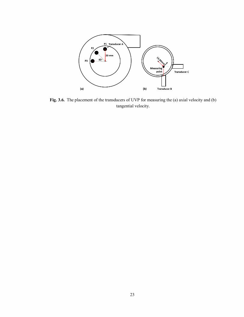
23

Fig. 3.6. The placement of the transducers of UVP for measuring the (a) axial velocity and (b) tangential velocity.

24

Chapter 4 Results and Discussion

4.1 Optimization of the TurboSwirl structure for uphill teeming

4.1.1 Validation and mesh sensitivity

The model was validated and mesh independent calculations were made in order to ensure that the results are accurate and trustworthy. The finite element analysis software, COMSOL Multiphysics®, was chosen for this simulation. The CFD module of COMSOL has only one type of k-ɛ based turbulence model, namely the standard k-ɛ turbulence model. Although some research has reported that the standard k-ɛ turbulence model often shows a poor agreement with experiment data [49], the simulation of the swirling flow by the standard k-ɛ turbulence model has been validated extensively by water model results of swirling flows for the casting process.[5-

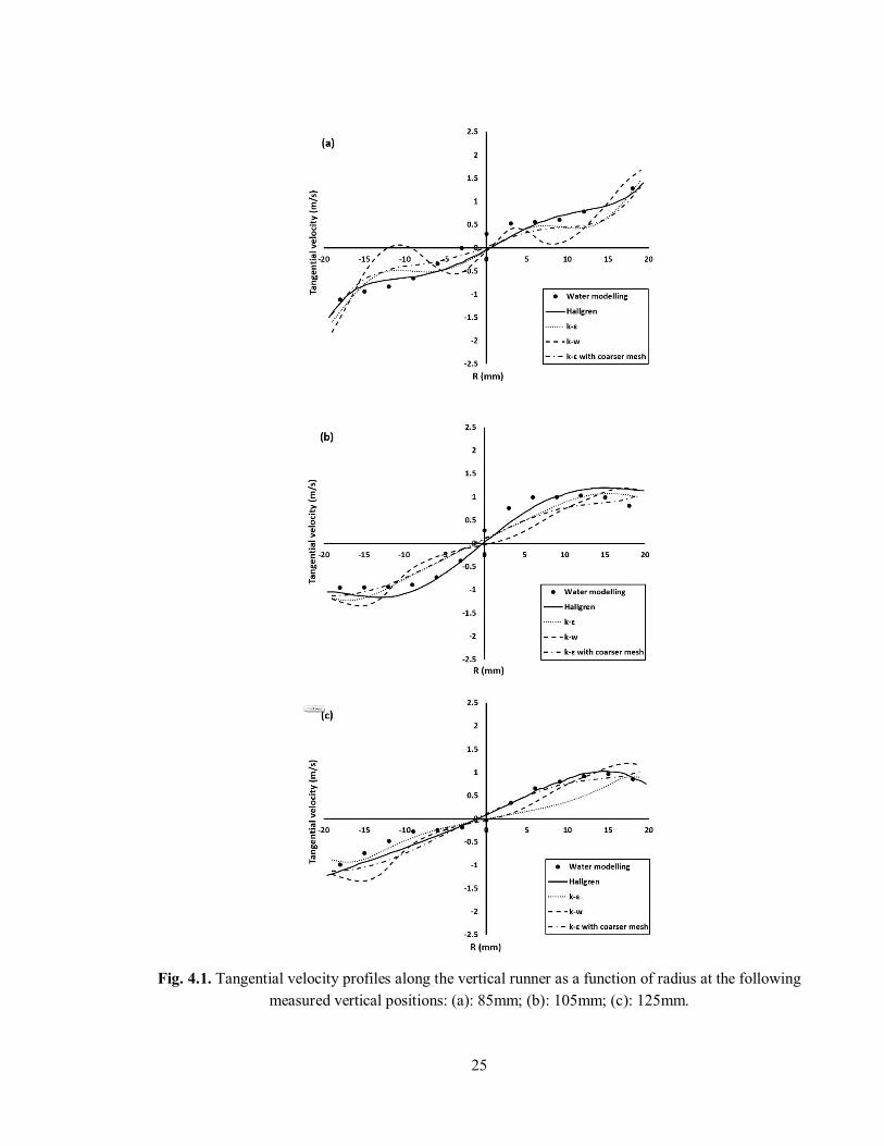
6, 8-9, 12] However, it is still necessary to test the feasibility of the standard k-ɛ turbulence model for simulating the swirling flow for the uphill teeming process. The simulation results obtained with COMSOL when using two turbulence models, k-ɛ and k-ω models with about 1.4 million cells, and with a coarser mesh with a similar number of cells in Hallgren’s simulation were compared with the simulation results and experimental data in Hallgren’s paper.[33] In this comparison, the swirling flow was generated by a swirl blade instead of by using a TurboSwirl device. Figure 4.1 shows the tangential velocity at three measured vertical positions (85mm, 105mm and 125mm) in the vertical runner. The results show that it is clear that the results of the k-ɛ model show an acceptable agreement with Hallgren’s simulation results as well as with the water modelling data, especially at the 85mm position. The k-ω model shows the worst agreement with the experiment data, and there is an obvious fluctuation, the largest difference from Hallgren’s simulation results being 298% greater than the difference of the k-ɛ model from Hallgren’s simulation results. Moreover, the tangential velocity of the coarser mesh of the k-ɛ model is quite close to the finer mesh in the centre part of runner at the 85 mm and 105 mm positions, but there is a 50%-200% greater difference than the finer mesh in the region close to the boundary layer at the 105 mm and 125 mm positions. In all three comparisons, the k-ɛ results are much closer to Hallgren’s results than the other two cases, and the trend is even more consistent in the experimental data. The k-ɛ turbulence model in COMSOL can thus effectively reflect the trend of a swirling flow and predict the flow pattern of a swirling flow.

25

Fig. 4.1. Tangential velocity profiles along the vertical runner as a function of radius at the following measured vertical positions: (a): 85mm; (b): 105mm; (c): 125mm.

26

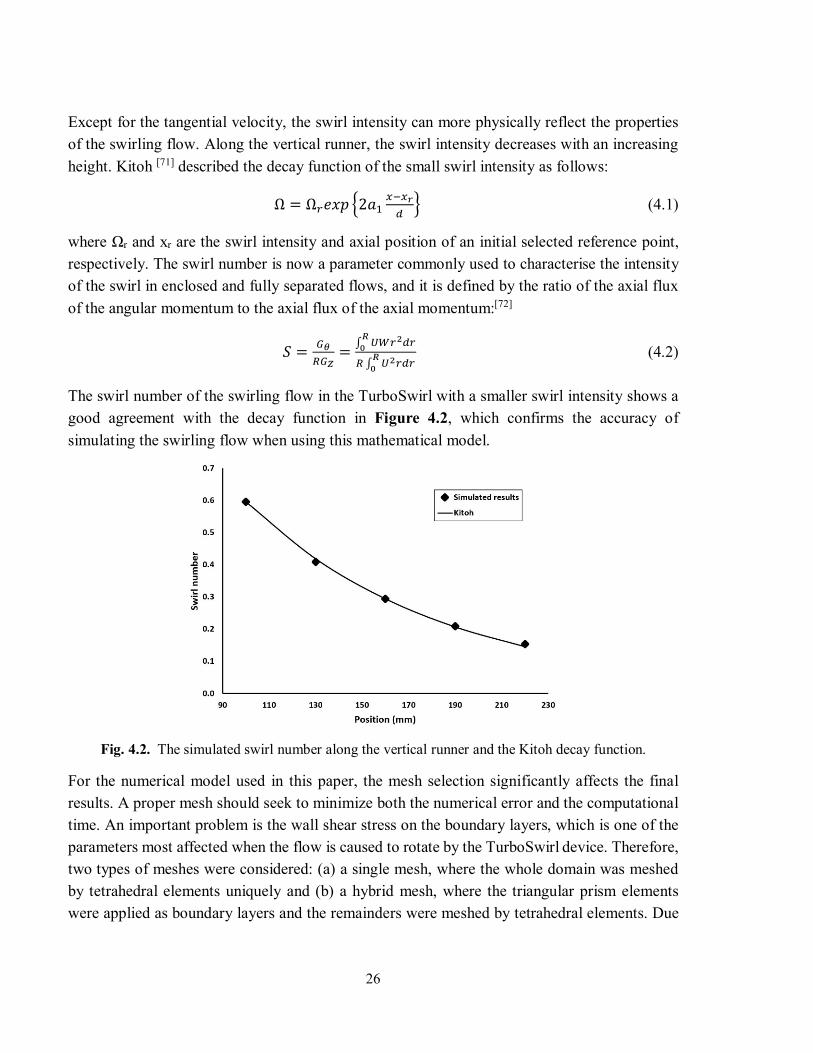
Except for the tangential velocity, the swirl intensity can more physically reflect the properties of the swirling flow. Along the vertical runner, the swirl intensity decreases with an increasing height. Kitoh [71] described the decay function of the small swirl intensity as follows:

Ω = Ω 2 (4.1)

where Ωr and xr are the swirl intensity and axial position of an initial selected reference point, respectively. The swirl number is now a parameter commonly used to characterise the intensity of the swirl in enclosed and fully separated flows, and it is defined by the ratio of the axial flux of the angular momentum to the axial flux of the axial momentum:[72]

= = ∫

∫ (4.2)

The swirl number of the swirling flow in the TurboSwirl with a smaller swirl intensity shows a good agreement with the decay function in Figure 4.2, which confirms the accuracy of simulating the swirling flow when using this mathematical model.

Fig. 4.2. The simulated swirl number along the vertical runner and the Kitoh decay function.

For the numerical model used in this paper, the mesh selection significantly affects the final results. A proper mesh should seek to minimize both the numerical error and the computational time. An important problem is the wall shear stress on the boundary layers, which is one of the parameters most affected when the flow is caused to rotate by the TurboSwirl device. Therefore, two types of meshes were considered: (a) a single mesh, where the whole domain was meshed by tetrahedral elements uniquely and (b) a hybrid mesh, where the triangular prism elements were applied as boundary layers and the remainders were meshed by tetrahedral elements. Due

27

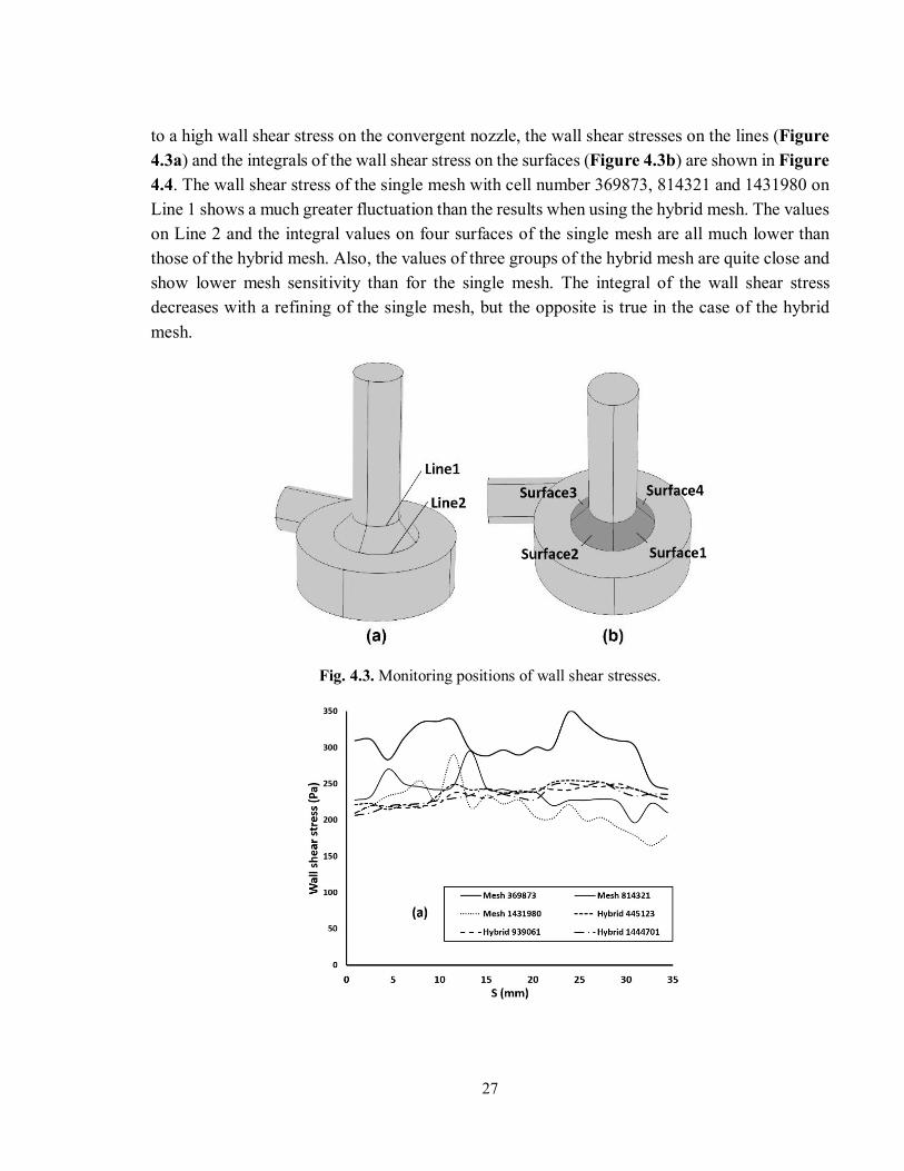
to a high wall shear stress on the convergent nozzle, the wall shear stresses on the lines (Figure 4.3a) and the integrals of the wall shear stress on the surfaces (Figure 4.3b) are shown in Figure 4.4. The wall shear stress of the single mesh with cell number 369873, 814321 and 1431980 on Line 1 shows a much greater fluctuation than the results when using the hybrid mesh. The values on Line 2 and the integral values on four surfaces of the single mesh are all much lower than those of the hybrid mesh. Also, the values of three groups of the hybrid mesh are quite close and show lower mesh sensitivity than for the single mesh. The integral of the wall shear stress decreases with a refining of the single mesh, but the opposite is true in the case of the hybrid mesh.

Fig. 4.3. Monitoring positions of wall shear stresses.

28

Fig. 4.4. (a): Wall shear stress on Line 1; (b): Wall shear stress on Line 2; (c): Integral of wall shear stress on Surfaces 1-4, according to Fig. 4.3.

The hybrid mesh shows a significant difference in the wall shear stress values on Line 2 and in the integral of the wall shear stress on all the surfaces. The numerical uncertainties due to the grid-spacing of the two mesh were calculated by using the GCI method [66] that can estimate the discretization error of a numerical solution. Table 4.1 shows the numerical uncertainties of the finest grid of the two meshes on Line 1-2 and Surface 1-4. The numerical uncertainties of the hybrid mesh are much smaller than those of the single mesh, because the existence of a boundary mesh can more effectively reflect the influence of the wall shear stress on the numerical results. Moreover, the axial velocity of the hybrid mesh is smaller than that of the single mesh with a similar number of cells, but the velocity of the hybrid mesh with 1444071 is much closer to that

29

of the single mesh with a finer grid. Therefore, the hybrid mesh with a cell number of 1444701 was selected for the continued study.

Table 4.1. Numerical uncertainties of the finest grid of two meshes.

Line 1

(Average value)

Line 2 (Average

value) Surface 1

Surface 2

Surface 3

Surface 4

Single mesh

9.59% 1.91% 78.35% 12.26% 41.34% 62.41%

Hybrid mesh

0.09% 1.17% 1.52% 6.27% 6.07% 2.22%

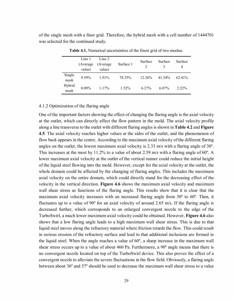
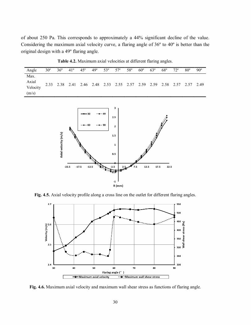
4.1.2 Optimization of the flaring angle

One of the important factors showing the effect of changing the flaring angle is the axial velocity at the outlet, which can directly affect the flow pattern in the mold. The axial velocity profile along a line transverse to the outlet with different flaring angles is shown in Table 4.2 and Figure 4.5. The axial velocity reaches higher values at the sides of the outlet, and the phenomenon of flow back appears in the centre. According to the maximum axial velocity of the different flaring angles on the outlet, the lowest maximum axial velocity is 2.33 m/s with a flaring angle of 30º. This increases at the most by 11.2% to a value of about 2.59 m/s with a flaring angle of 60º. A lower maximum axial velocity at the outlet of the vertical runner could reduce the initial height of the liquid steel flowing into the mold. However, except for the axial velocity at the outlet, the whole domain could be affected by the changing of flaring angles. This includes the maximum axial velocity on the entire domain, which could directly stand for the decreasing effect of the velocity in the vertical direction. Figure 4.6 shows the maximum axial velocity and maximum wall shear stress as functions of the flaring angle. This results show that it is clear that the maximum axial velocity increases with an increased flaring angle from 30º to 60º. Then, it fluctuates up to a value of 90º for an axial velocity of around 2.65 m/s. If the flaring angle is decreased further, which corresponds to an enlarged convergent nozzle to the edge of the TurboSwirl, a much lower maximum axial velocity could be obtained. However, Figure 4.6 also shows that a low flaring angle leads to a high maximum wall shear stress. This is due to that liquid steel moves along the refractory material where friction retards the flow. This could result in serious erosion of the refractory surface and lead to that additional inclusions are formed in the liquid steel. When the angle reaches a value of 60º, a sharp increase in the maximum wall shear stress occurs up to a value of about 460 Pa. Furthermore, a 90º angle means that there is no convergent nozzle located on top of the TurboSwirl device. This also proves the effect of a convergent nozzle to alleviate the severe fluctuations in the flow field. Obviously, a flaring angle between about 36º and 57º should be used to decrease the maximum wall shear stress to a value

30

of about 250 Pa. This corresponds to approximately a 44% significant decline of the value. Considering the maximum axial velocity curve, a flaring angle of 36º to 40º is better than the original design with a 49º flaring angle.

Table 4.2. Maximum axial velocities at different flaring angles.

Angle 30º 36º 41º 45º 49º 53º 57º 58º 60º 63º 68º 72º 80º 90º Max. Axial Velocity (m/s)

2.33 2.38 2.41 2.46 2.48 2.53 2.55 2.57 2.59 2.59 2.58 2.57 2.57 2.49

Fig. 4.5. Axial velocity profile along a cross line on the outlet for different flaring angles.

Fig. 4.6. Maximum axial velocity and maximum wall shear stress as functions of flaring angle.

31

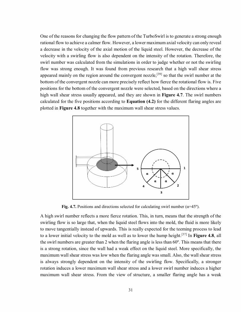
One of the reasons for changing the flow pattern of the TurboSwirl is to generate a strong enough rational flow to achieve a calmer flow. However, a lower maximum axial velocity can only reveal a decrease in the velocity of the axial motion of the liquid steel. However, the decrease of the velocity with a swirling flow is also dependent on the intensity of the rotation. Therefore, the swirl number was calculated from the simulations in order to judge whether or not the swirling flow was strong enough. It was found from previous research that a high wall shear stress appeared mainly on the region around the convergent nozzle,[39] so that the swirl number at the bottom of the convergent nozzle can more precisely reflect how fierce the rotational flow is. Five positions for the bottom of the convergent nozzle were selected, based on the directions where a high wall shear stress usually appeared, and they are shown in Figure 4.7. The swirl numbers calculated for the five positions according to Equation (4.2) for the different flaring angles are plotted in Figure 4.8 together with the maximum wall shear stress values.

Fig. 4.7. Positions and directions selected for calculating swirl number (α=45º).

A high swirl number reflects a more fierce rotation. This, in turn, means that the strength of the swirling flow is so large that, when the liquid steel flows into the mold, the fluid is more likely to move tangentially instead of upwards. This is really expected for the teeming process to lead to a lower initial velocity to the mold as well as to lower the hump height.[37] In Figure 4.8, all the swirl numbers are greater than 2 when the flaring angle is less than 60º. This means that there is a strong rotation, since the wall had a weak effect on the liquid steel. More specifically, the maximum wall shear stress was low when the flaring angle was small. Also, the wall shear stress is always strongly dependent on the intensity of the swirling flow. Specifically, a stronger rotation induces a lower maximum wall shear stress and a lower swirl number induces a higher maximum wall shear stress. From the view of structure, a smaller flaring angle has a weak

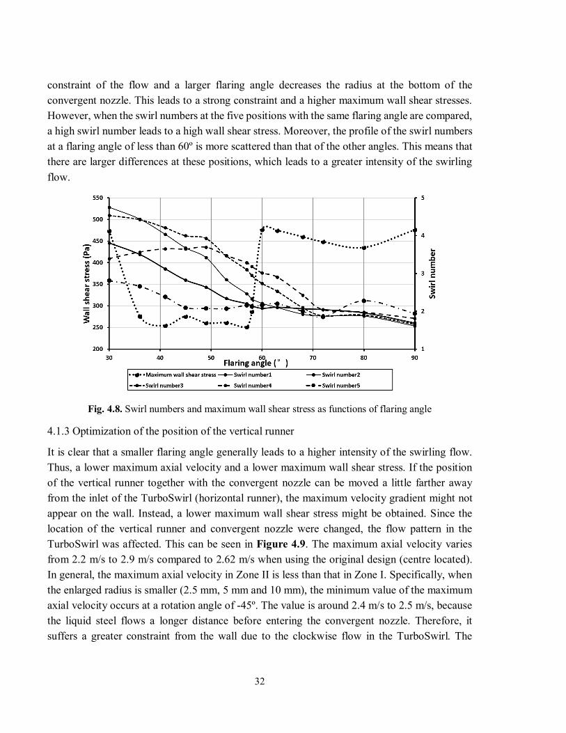
32

constraint of the flow and a larger flaring angle decreases the radius at the bottom of the convergent nozzle. This leads to a strong constraint and a higher maximum wall shear stresses. However, when the swirl numbers at the five positions with the same flaring angle are compared, a high swirl number leads to a high wall shear stress. Moreover, the profile of the swirl numbers at a flaring angle of less than 60º is more scattered than that of the other angles. This means that there are larger differences at these positions, which leads to a greater intensity of the swirling flow.

Fig. 4.8. Swirl numbers and maximum wall shear stress as functions of flaring angle

4.1.3 Optimization of the position of the vertical runner

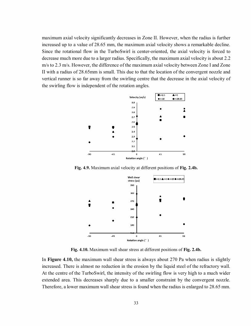
It is clear that a smaller flaring angle generally leads to a higher intensity of the swirling flow. Thus, a lower maximum axial velocity and a lower maximum wall shear stress. If the position of the vertical runner together with the convergent nozzle can be moved a little farther away from the inlet of the TurboSwirl (horizontal runner), the maximum velocity gradient might not appear on the wall. Instead, a lower maximum wall shear stress might be obtained. Since the location of the vertical runner and convergent nozzle were changed, the flow pattern in the TurboSwirl was affected. This can be seen in Figure 4.9. The maximum axial velocity varies from 2.2 m/s to 2.9 m/s compared to 2.62 m/s when using the original design (centre located). In general, the maximum axial velocity in Zone II is less than that in Zone I. Specifically, when the enlarged radius is smaller (2.5 mm, 5 mm and 10 mm), the minimum value of the maximum axial velocity occurs at a rotation angle of -45º. The value is around 2.4 m/s to 2.5 m/s, because the liquid steel flows a longer distance before entering the convergent nozzle. Therefore, it suffers a greater constraint from the wall due to the clockwise flow in the TurboSwirl. The

33

maximum axial velocity significantly decreases in Zone II. However, when the radius is further increased up to a value of 28.65 mm, the maximum axial velocity shows a remarkable decline. Since the rotational flow in the TurboSwirl is center-oriented, the axial velocity is forced to decrease much more due to a larger radius. Specifically, the maximum axial velocity is about 2.2 m/s to 2.3 m/s. However, the difference of the maximum axial velocity between Zone I and Zone II with a radius of 28.65mm is small. This due to that the location of the convergent nozzle and vertical runner is so far away from the swirling centre that the decrease in the axial velocity of the swirling flow is independent of the rotation angles.

Fig. 4.9. Maximum axial velocity at different positions of Fig. 2.4b.

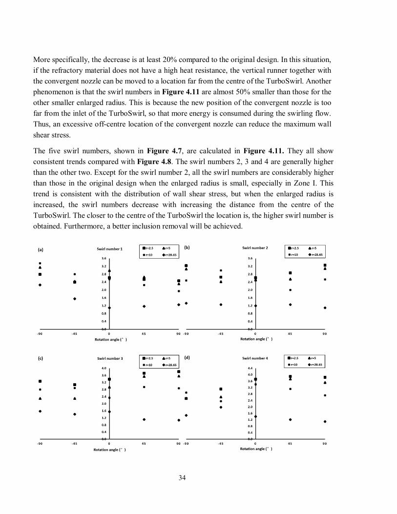
Fig. 4.10. Maximum wall shear stress at different positions of Fig. 2.4b.

In Figure 4.10, the maximum wall shear stress is always about 270 Pa when radius is slightly increased. There is almost no reduction in the erosion by the liquid steel of the refractory wall. At the centre of the TurboSwirl, the intensity of the swirling flow is very high to a much wider extended area. This decreases sharply due to a smaller constraint by the convergent nozzle. Therefore, a lower maximum wall shear stress is found when the radius is enlarged to 28.65 mm.

34

More specifically, the decrease is at least 20% compared to the original design. In this situation, if the refractory material does not have a high heat resistance, the vertical runner together with the convergent nozzle can be moved to a location far from the centre of the TurboSwirl. Another phenomenon is that the swirl numbers in Figure 4.11 are almost 50% smaller than those for the other smaller enlarged radius. This is because the new position of the convergent nozzle is too far from the inlet of the TurboSwirl, so that more energy is consumed during the swirling flow. Thus, an excessive off-centre location of the convergent nozzle can reduce the maximum wall shear stress.

The five swirl numbers, shown in Figure 4.7, are calculated in Figure 4.11. They all show consistent trends compared with Figure 4.8. The swirl numbers 2, 3 and 4 are generally higher than the other two. Except for the swirl number 2, all the swirl numbers are considerably higher than those in the original design when the enlarged radius is small, especially in Zone I. This trend is consistent with the distribution of wall shear stress, but when the enlarged radius is increased, the swirl numbers decrease with increasing the distance from the centre of the TurboSwirl. The closer to the centre of the TurboSwirl the location is, the higher swirl number is obtained. Furthermore, a better inclusion removal will be achieved.

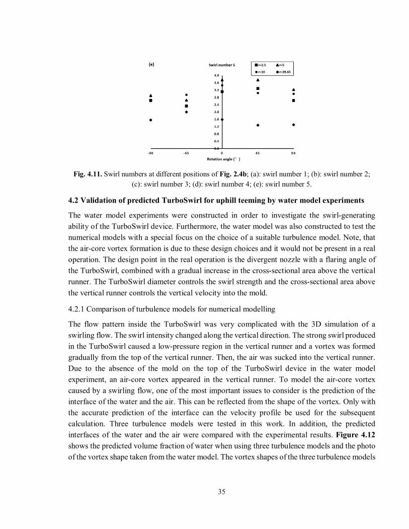
35

Fig. 4.11. Swirl numbers at different positions of Fig. 2.4b; (a): swirl number 1; (b): swirl number 2; (c): swirl number 3; (d): swirl number 4; (e): swirl number 5.

4.2 Validation of predicted TurboSwirl for uphill teeming by water model experiments

The water model experiments were constructed in order to investigate the swirl-generating ability of the TurboSwirl device. Furthermore, the water model was also constructed to test the numerical models with a special focus on the choice of a suitable turbulence model. Note, that the air-core vortex formation is due to these design choices and it would not be present in a real operation. The design point in the real operation is the divergent nozzle with a flaring angle of the TurboSwirl, combined with a gradual increase in the cross-sectional area above the vertical runner. The TurboSwirl diameter controls the swirl strength and the cross-sectional area above the vertical runner controls the vertical velocity into the mold.

4.2.1 Comparison of turbulence models for numerical modelling

The flow pattern inside the TurboSwirl was very complicated with the 3D simulation of a swirling flow. The swirl intensity changed along the vertical direction. The strong swirl produced in the TurboSwirl caused a low-pressure region in the vertical runner and a vortex was formed gradually from the top of the vertical runner. Then, the air was sucked into the vertical runner. Due to the absence of the mold on the top of the TurboSwirl device in the water model experiment, an air-core vortex appeared in the vertical runner. To model the air-core vortex caused by a swirling flow, one of the most important issues to consider is the prediction of the interface of the water and the air. This can be reflected from the shape of the vortex. Only with the accurate prediction of the interface can the velocity profile be used for the subsequent calculation. Three turbulence models were tested in this work. In addition, the predicted interfaces of the water and the air were compared with the experimental results. Figure 4.12 shows the predicted volume fraction of water when using three turbulence models and the photo of the vortex shape taken from the water model. The vortex shapes of the three turbulence models

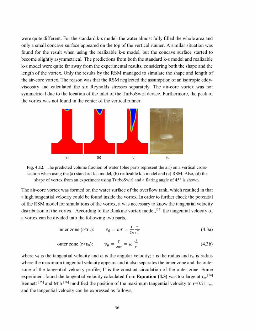
36

were quite different. For the standard k-ε model, the water almost fully filled the whole area and only a small concave surface appeared on the top of the vertical runner. A similar situation was found for the result when using the realizable k-ε model, but the concave surface started to become slightly asymmetrical. The predictions from both the standard k-ε model and realizable k-ε model were quite far away from the experimental results, considering both the shape and the length of the vortex. Only the results by the RSM managed to simulate the shape and length of the air-core vortex. The reason was that the RSM neglected the assumption of an isotropic eddy-viscosity and calculated the six Reynolds stresses separately. The air-core vortex was not symmetrical due to the location of the inlet of the TurboSwirl device. Furthermore, the peak of the vortex was not found in the center of the vertical runner.

Fig. 4.12. The predicted volume fraction of water (blue parts represent the air) on a vertical cross-section when using the (a) standard k-ε model, (b) realizable k-ε model and (c) RSM. Also, (d) the

shape of vortex from an experiment using TurboSwirl and a flaring angle of 45° is shown.

The air-core vortex was formed on the water surface of the overflow tank, which resulted in that a high tangential velocity could be found inside the vortex. In order to further check the potential of the RSM model for simulations of the vortex, it was necessary to know the tangential velocity distribution of the vortex. According to the Rankine vortex model,[73] the tangential velocity of a vortex can be divided into the following two parts,

inner zone (r<rm): = = (4.3a)

outer zone (r>rm): = = (4.3b)

where vθ is the tangential velocity and ω is the angular velocity; r is the radius and rm is radius where the maximum tangential velocity appears and it also separates the inner zone and the outer zone of the tangential velocity profile; Γ is the constant circulation of the outer zone. Some experiment found the tangential velocity calculated from Equation (4.3) was too large at rm.[74] Bennett [75] and Mih [76] modified the position of the maximum tangential velocity to r=0.71 rm, and the tangential velocity can be expressed as follows,

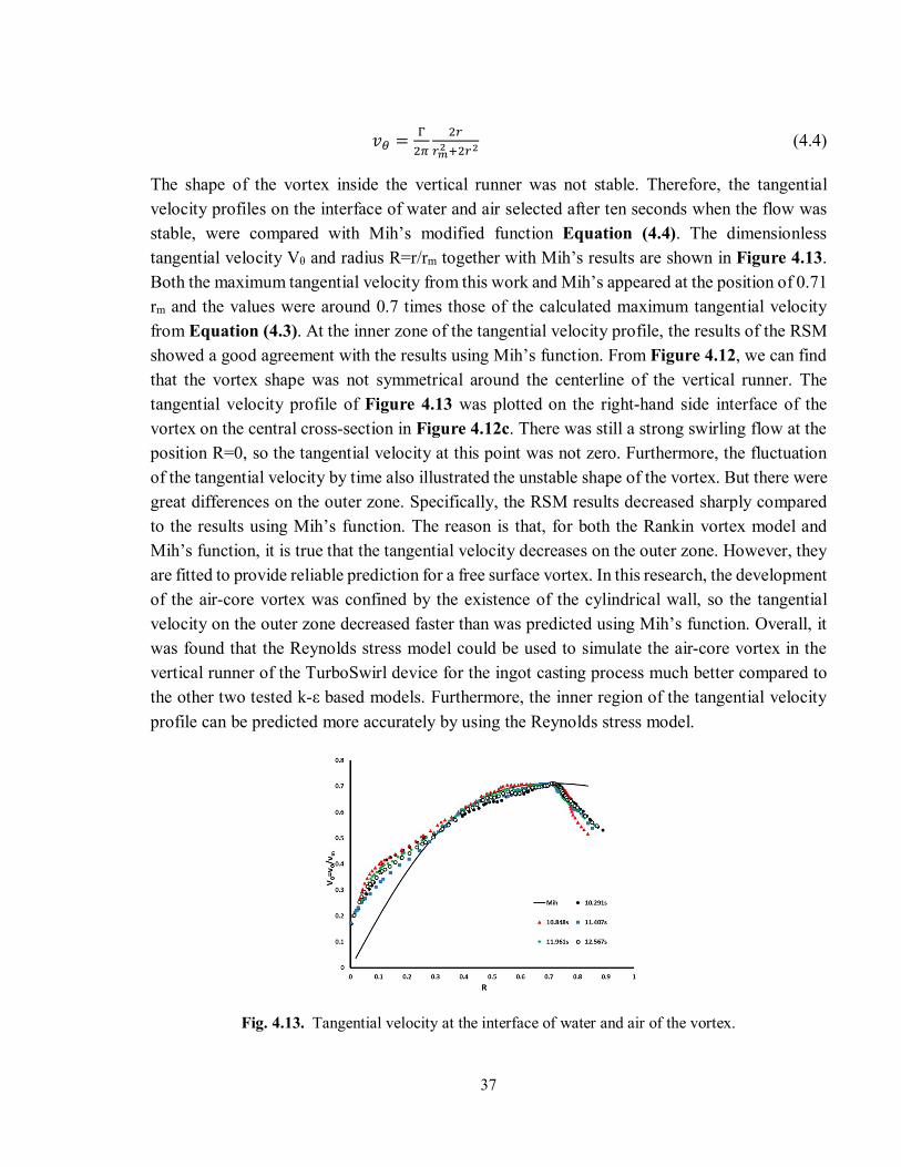
37

= (4.4)

The shape of the vortex inside the vertical runner was not stable. Therefore, the tangential velocity profiles on the interface of water and air selected after ten seconds when the flow was stable, were compared with Mih’s modified function Equation (4.4). The dimensionless tangential velocity Vθ and radius R=r/rm together with Mih’s results are shown in Figure 4.13. Both the maximum tangential velocity from this work and Mih’s appeared at the position of 0.71 rm and the values were around 0.7 times those of the calculated maximum tangential velocity from Equation (4.3). At the inner zone of the tangential velocity profile, the results of the RSM showed a good agreement with the results using Mih’s function. From Figure 4.12, we can find that the vortex shape was not symmetrical around the centerline of the vertical runner. The tangential velocity profile of Figure 4.13 was plotted on the right-hand side interface of the vortex on the central cross-section in Figure 4.12c. There was still a strong swirling flow at the position R=0, so the tangential velocity at this point was not zero. Furthermore, the fluctuation of the tangential velocity by time also illustrated the unstable shape of the vortex. But there were great differences on the outer zone. Specifically, the RSM results decreased sharply compared to the results using Mih’s function. The reason is that, for both the Rankin vortex model and Mih’s function, it is true that the tangential velocity decreases on the outer zone. However, they are fitted to provide reliable prediction for a free surface vortex. In this research, the development of the air-core vortex was confined by the existence of the cylindrical wall, so the tangential velocity on the outer zone decreased faster than was predicted using Mih’s function. Overall, it was found that the Reynolds stress model could be used to simulate the air-core vortex in the vertical runner of the TurboSwirl device for the ingot casting process much better compared to the other two tested k-ε based models. Furthermore, the inner region of the tangential velocity profile can be predicted more accurately by using the Reynolds stress model.

Fig. 4.13. Tangential velocity at the interface of water and air of the vortex.

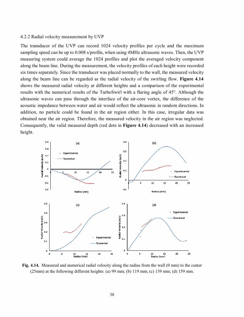
38

4.2.2 Radial velocity measurement by UVP

The transducer of the UVP can record 1024 velocity profiles per cycle and the maximum sampling speed can be up to 0.008 s/profile, when using 4MHz ultrasonic waves. Then, the UVP measuring system could average the 1024 profiles and plot the averaged velocity component along the beam line. During the measurement, the velocity profiles of each height were recorded six times separately. Since the transducer was placed normally to the wall, the measured velocity along the beam line can be regarded as the radial velocity of the swirling flow. Figure 4.14 shows the measured radial velocity at different heights and a comparison of the experimental results with the numerical results of the TurboSwirl with a flaring angle of 45°. Although the ultrasonic waves can pass through the interface of the air-core vortex, the difference of the acoustic impedance between water and air would reflect the ultrasonic in random directions. In addition, no particle could be found in the air region either. In this case, irregular data was obtained near the air region. Therefore, the measured velocity in the air region was neglected. Consequently, the valid measured depth (red dots in Figure 4.14) decreased with an increased height.

Fig. 4.14. Measured and numerical radial velocity along the radius from the wall (0 mm) to the center (25mm) at the following different heights: (a) 99 mm; (b) 119 mm; (c) 139 mm; (d) 159 mm.

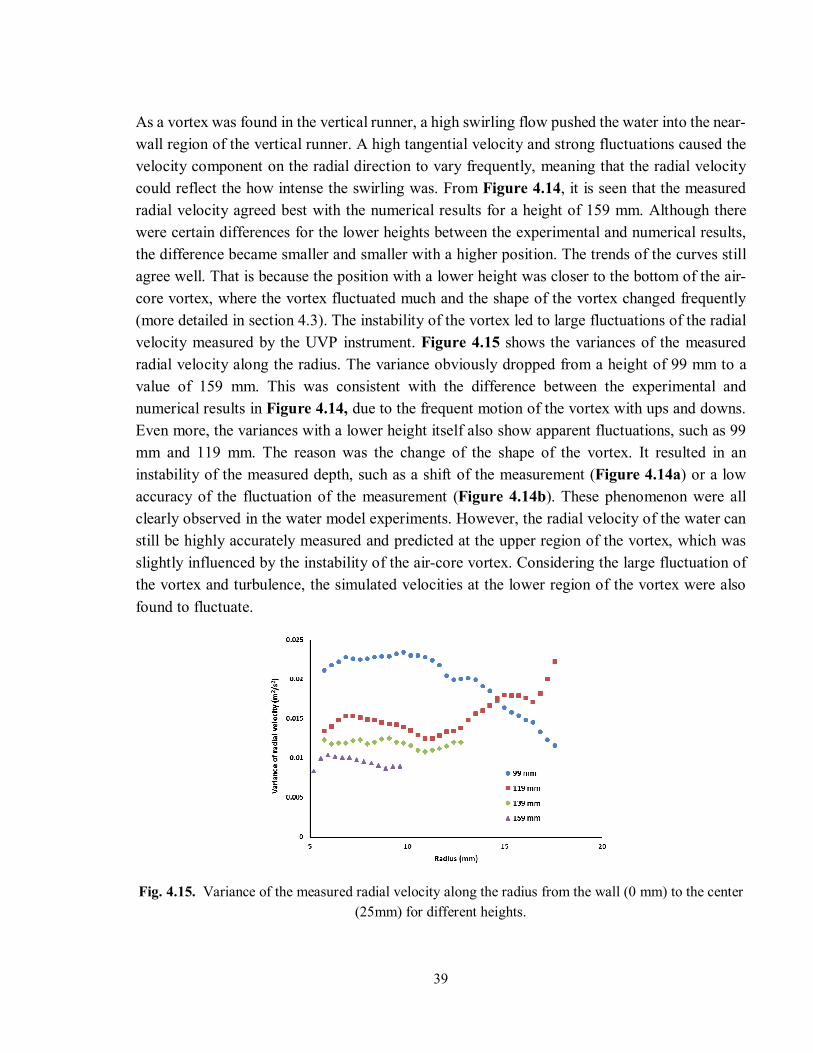
39

As a vortex was found in the vertical runner, a high swirling flow pushed the water into the near-wall region of the vertical runner. A high tangential velocity and strong fluctuations caused the velocity component on the radial direction to vary frequently, meaning that the radial velocity could reflect the how intense the swirling was. From Figure 4.14, it is seen that the measured radial velocity agreed best with the numerical results for a height of 159 mm. Although there were certain differences for the lower heights between the experimental and numerical results, the difference became smaller and smaller with a higher position. The trends of the curves still agree well. That is because the position with a lower height was closer to the bottom of the air-core vortex, where the vortex fluctuated much and the shape of the vortex changed frequently (more detailed in section 4.3). The instability of the vortex led to large fluctuations of the radial velocity measured by the UVP instrument. Figure 4.15 shows the variances of the measured radial velocity along the radius. The variance obviously dropped from a height of 99 mm to a value of 159 mm. This was consistent with the difference between the experimental and numerical results in Figure 4.14, due to the frequent motion of the vortex with ups and downs. Even more, the variances with a lower height itself also show apparent fluctuations, such as 99 mm and 119 mm. The reason was the change of the shape of the vortex. It resulted in an instability of the measured depth, such as a shift of the measurement (Figure 4.14a) or a low accuracy of the fluctuation of the measurement (Figure 4.14b). These phenomenon were all clearly observed in the water model experiments. However, the radial velocity of the water can still be highly accurately measured and predicted at the upper region of the vortex, which was slightly influenced by the instability of the air-core vortex. Considering the large fluctuation of the vortex and turbulence, the simulated velocities at the lower region of the vortex were also found to fluctuate.

Fig. 4.15. Variance of the measured radial velocity along the radius from the wall (0 mm) to the center (25mm) for different heights.

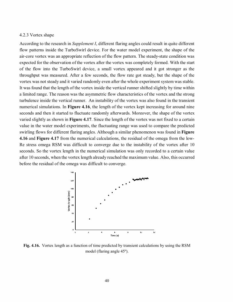
40

4.2.3 Vortex shape

According to the research in Supplement I, different flaring angles could result in quite different flow patterns inside the TurboSwirl device. For the water model experiment, the shape of the air-core vortex was an appropriate reflection of the flow pattern. The steady-state condition was expected for the observation of the vortex after the vortex was completely formed. With the start of the flow into the TurboSwirl device, a small vortex appeared and it got stronger as the throughput was measured. After a few seconds, the flow rate got steady, but the shape of the vortex was not steady and it varied randomly even after the whole experiment system was stable. It was found that the length of the vortex inside the vertical runner shifted slightly by time within a limited range. The reason was the asymmetric flow characteristics of the vortex and the strong turbulence inside the vertical runner. An instability of the vortex was also found in the transient numerical simulations. In Figure 4.16, the length of the vortex kept increasing for around nine seconds and then it started to fluctuate randomly afterwards. Moreover, the shape of the vortex varied slightly as shown in Figure 4.17. Since the length of the vortex was not fixed to a certain value in the water model experiments, the fluctuating range was used to compare the predicted swirling flows for different flaring angles. Although a similar phenomenon was found in Figure 4.16 and Figure 4.17 from the numerical calculations, the residual of the omega from the low-Re stress omega RSM was difficult to converge due to the instability of the vortex after 10 seconds. So the vortex length in the numerical simulation was only recorded to a certain value after 10 seconds, when the vortex length already reached the maximum value. Also, this occurred before the residual of the omega was difficult to converge.

Fig. 4.16. Vortex length as a function of time predicted by transient calculations by using the RSM model (flaring angle 45º).

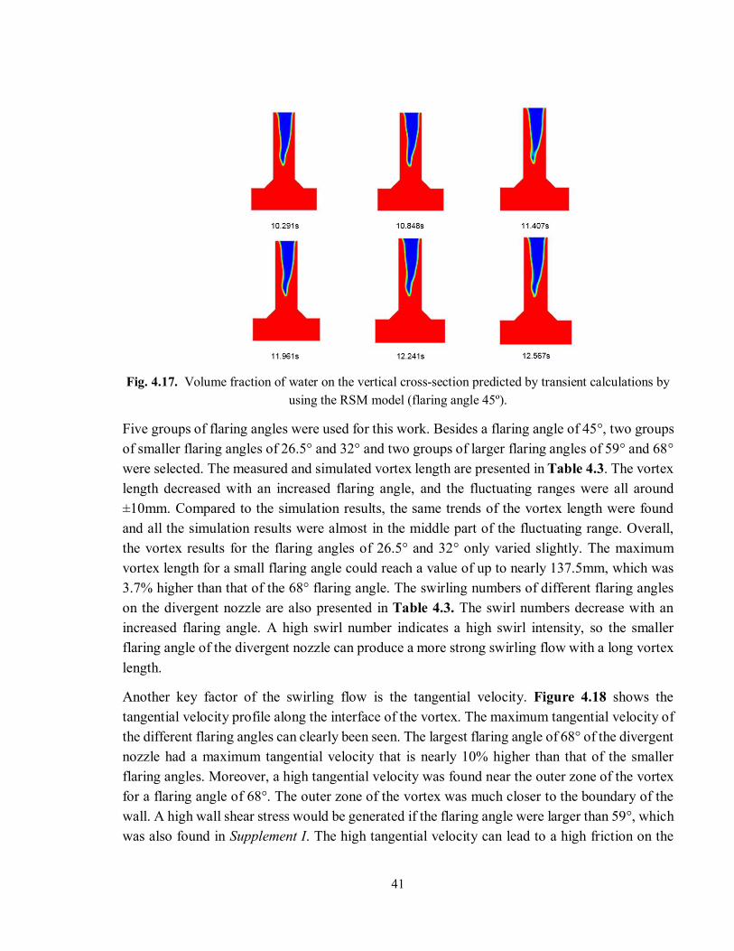
41

Fig. 4.17. Volume fraction of water on the vertical cross-section predicted by transient calculations by using the RSM model (flaring angle 45º).

Five groups of flaring angles were used for this work. Besides a flaring angle of 45°, two groups of smaller flaring angles of 26.5° and 32° and two groups of larger flaring angles of 59° and 68° were selected. The measured and simulated vortex length are presented in Table 4.3. The vortex length decreased with an increased flaring angle, and the fluctuating ranges were all around ±10mm. Compared to the simulation results, the same trends of the vortex length were found and all the simulation results were almost in the middle part of the fluctuating range. Overall, the vortex results for the flaring angles of 26.5° and 32° only varied slightly. The maximum vortex length for a small flaring angle could reach a value of up to nearly 137.5mm, which was 3.7% higher than that of the 68° flaring angle. The swirling numbers of different flaring angles on the divergent nozzle are also presented in Table 4.3. The swirl numbers decrease with an increased flaring angle. A high swirl number indicates a high swirl intensity, so the smaller flaring angle of the divergent nozzle can produce a more strong swirling flow with a long vortex length.

Another key factor of the swirling flow is the tangential velocity. Figure 4.18 shows the tangential velocity profile along the interface of the vortex. The maximum tangential velocity of the different flaring angles can clearly been seen. The largest flaring angle of 68° of the divergent nozzle had a maximum tangential velocity that is nearly 10% higher than that of the smaller flaring angles. Moreover, a high tangential velocity was found near the outer zone of the vortex for a flaring angle of 68°. The outer zone of the vortex was much closer to the boundary of the wall. A high wall shear stress would be generated if the flaring angle were larger than 59°, which was also found in Supplement I. The high tangential velocity can lead to a high friction on the

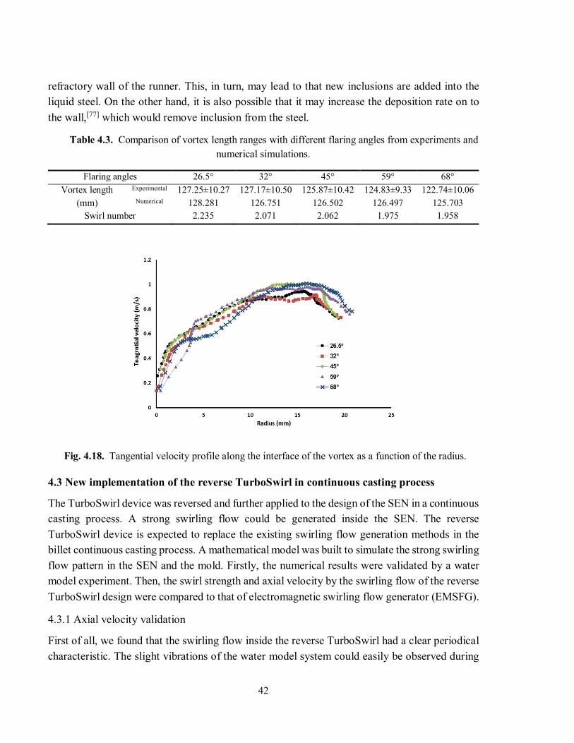
42

refractory wall of the runner. This, in turn, may lead to that new inclusions are added into the liquid steel. On the other hand, it is also possible that it may increase the deposition rate on to the wall,[77] which would remove inclusion from the steel.

Table 4.3. Comparison of vortex length ranges with different flaring angles from experiments and numerical simulations.

Flaring angles 26.5° 32° 45° 59° 68° Vortex length

(mm)

Experimental 127.25±10.27 127.17±10.50 125.87±10.42 124.83±9.33 122.74±10.06 Numerical 128.281 126.751 126.502 126.497 125.703

Swirl number 2.235 2.071 2.062 1.975 1.958

Fig. 4.18. Tangential velocity profile along the interface of the vortex as a function of the radius.

4.3 New implementation of the reverse TurboSwirl in continuous casting process

The TurboSwirl device was reversed and further applied to the design of the SEN in a continuous casting process. A strong swirling flow could be generated inside the SEN. The reverse TurboSwirl device is expected to replace the existing swirling flow generation methods in the billet continuous casting process. A mathematical model was built to simulate the strong swirling flow pattern in the SEN and the mold. Firstly, the numerical results were validated by a water model experiment. Then, the swirl strength and axial velocity by the swirling flow of the reverse TurboSwirl design were compared to that of electromagnetic swirling flow generator (EMSFG).

4.3.1 Axial velocity validation

First of all, we found that the swirling flow inside the reverse TurboSwirl had a clear periodical characteristic. The slight vibrations of the water model system could easily be observed during

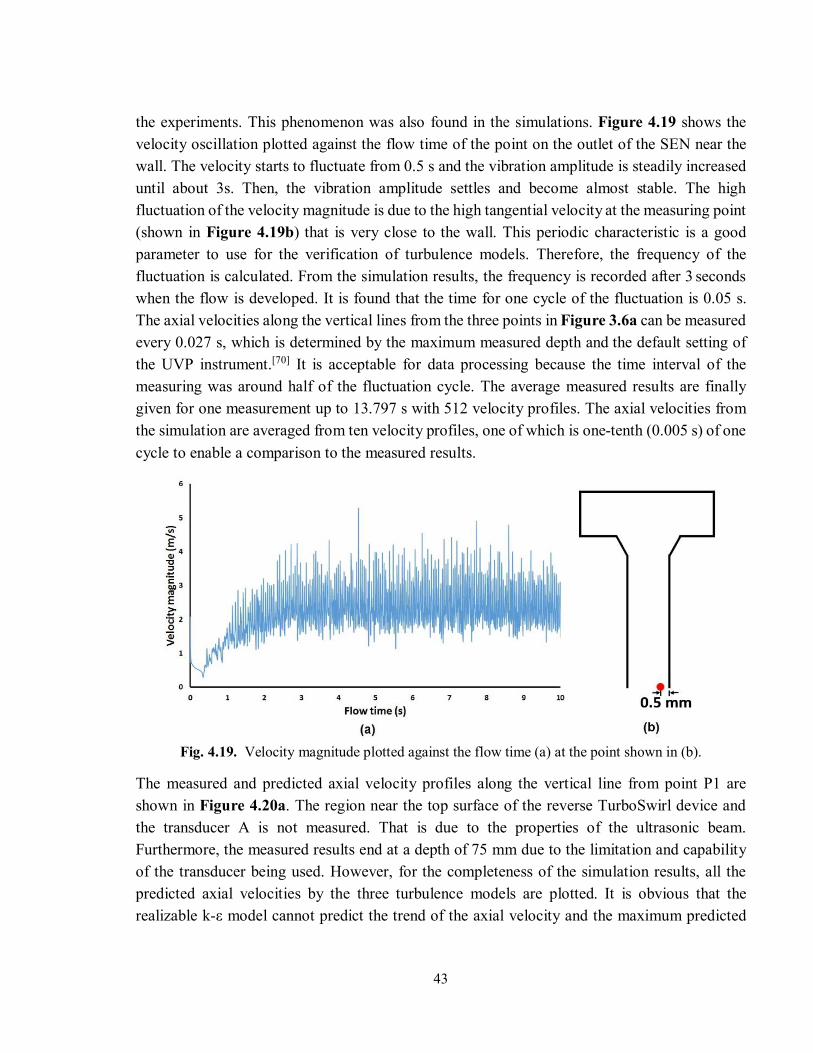
43

the experiments. This phenomenon was also found in the simulations. Figure 4.19 shows the velocity oscillation plotted against the flow time of the point on the outlet of the SEN near the wall. The velocity starts to fluctuate from 0.5 s and the vibration amplitude is steadily increased until about 3s. Then, the vibration amplitude settles and become almost stable. The high fluctuation of the velocity magnitude is due to the high tangential velocity at the measuring point (shown in Figure 4.19b) that is very close to the wall. This periodic characteristic is a good parameter to use for the verification of turbulence models. Therefore, the frequency of the fluctuation is calculated. From the simulation results, the frequency is recorded after 3 seconds when the flow is developed. It is found that the time for one cycle of the fluctuation is 0.05 s. The axial velocities along the vertical lines from the three points in Figure 3.6a can be measured every 0.027 s, which is determined by the maximum measured depth and the default setting of the UVP instrument.[70] It is acceptable for data processing because the time interval of the measuring was around half of the fluctuation cycle. The average measured results are finally given for one measurement up to 13.797 s with 512 velocity profiles. The axial velocities from the simulation are averaged from ten velocity profiles, one of which is one-tenth (0.005 s) of one cycle to enable a comparison to the measured results.

Fig. 4.19. Velocity magnitude plotted against the flow time (a) at the point shown in (b).

The measured and predicted axial velocity profiles along the vertical line from point P1 are shown in Figure 4.20a. The region near the top surface of the reverse TurboSwirl device and the transducer A is not measured. That is due to the properties of the ultrasonic beam. Furthermore, the measured results end at a depth of 75 mm due to the limitation and capability of the transducer being used. However, for the completeness of the simulation results, all the predicted axial velocities by the three turbulence models are plotted. It is obvious that the realizable k-ε model cannot predict the trend of the axial velocity and the maximum predicted

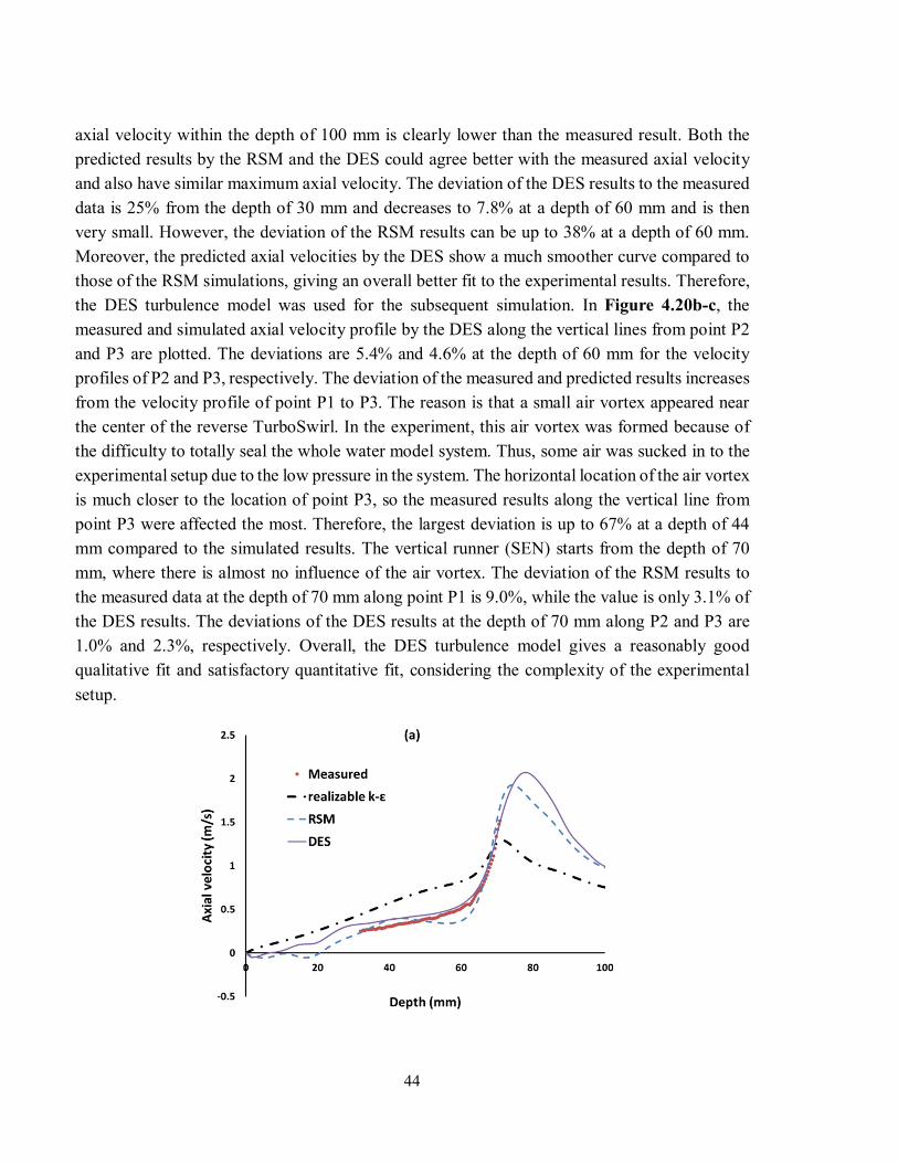
44

axial velocity within the depth of 100 mm is clearly lower than the measured result. Both the predicted results by the RSM and the DES could agree better with the measured axial velocity and also have similar maximum axial velocity. The deviation of the DES results to the measured data is 25% from the depth of 30 mm and decreases to 7.8% at a depth of 60 mm and is then very small. However, the deviation of the RSM results can be up to 38% at a depth of 60 mm. Moreover, the predicted axial velocities by the DES show a much smoother curve compared to those of the RSM simulations, giving an overall better fit to the experimental results. Therefore, the DES turbulence model was used for the subsequent simulation. In Figure 4.20b-c, the measured and simulated axial velocity profile by the DES along the vertical lines from point P2 and P3 are plotted. The deviations are 5.4% and 4.6% at the depth of 60 mm for the velocity profiles of P2 and P3, respectively. The deviation of the measured and predicted results increases from the velocity profile of point P1 to P3. The reason is that a small air vortex appeared near the center of the reverse TurboSwirl. In the experiment, this air vortex was formed because of the difficulty to totally seal the whole water model system. Thus, some air was sucked in to the experimental setup due to the low pressure in the system. The horizontal location of the air vortex is much closer to the location of point P3, so the measured results along the vertical line from point P3 were affected the most. Therefore, the largest deviation is up to 67% at a depth of 44 mm compared to the simulated results. The vertical runner (SEN) starts from the depth of 70 mm, where there is almost no influence of the air vortex. The deviation of the RSM results to the measured data at the depth of 70 mm along point P1 is 9.0%, while the value is only 3.1% of the DES results. The deviations of the DES results at the depth of 70 mm along P2 and P3 are 1.0% and 2.3%, respectively. Overall, the DES turbulence model gives a reasonably good qualitative fit and satisfactory quantitative fit, considering the complexity of the experimental setup.

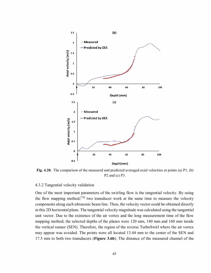
45

Fig. 4.20. The comparison of the measured and predicted averaged axial velocities at points (a) P1, (b)

P2 and (c) P3.

4.3.2 Tangential velocity validation

One of the most important parameters of the swirling flow is the tangential velocity. By using the flow mapping method,[70] two transducer work at the same time to measure the velocity components along each ultrasonic beam line. Then, the velocity vector could be obtained directly in this 2D horizontal plane. The tangential velocity magnitude was calculated using the tangential unit vector. Due to the existence of the air vortex and the long measurement time of the flow mapping method, the selected depths of the planes were 120 mm, 140 mm and 160 mm inside the vertical runner (SEN). Therefore, the region of the reverse TurboSwirl where the air vortex may appear was avoided. The points were all located 13.44 mm to the center of the SEN and 17.5 mm to both two transducers (Figure 3.6b). The distance of the measured channel of the

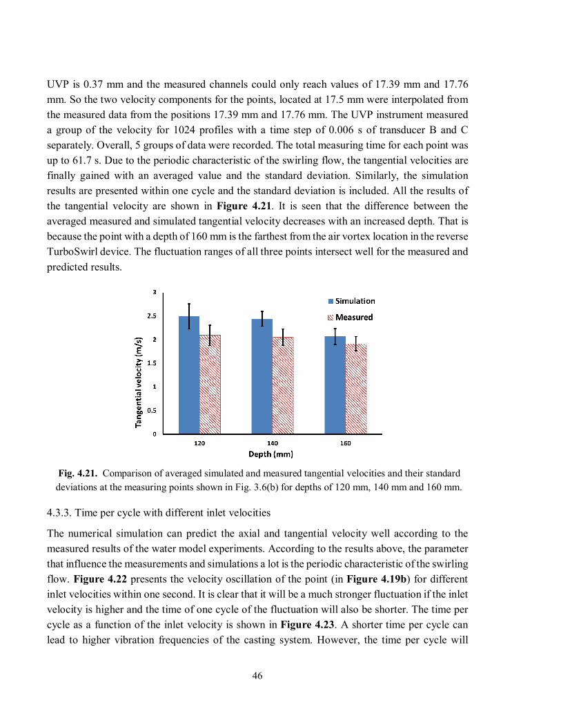
46

UVP is 0.37 mm and the measured channels could only reach values of 17.39 mm and 17.76 mm. So the two velocity components for the points, located at 17.5 mm were interpolated from the measured data from the positions 17.39 mm and 17.76 mm. The UVP instrument measured a group of the velocity for 1024 profiles with a time step of 0.006 s of transducer B and C separately. Overall, 5 groups of data were recorded. The total measuring time for each point was up to 61.7 s. Due to the periodic characteristic of the swirling flow, the tangential velocities are finally gained with an averaged value and the standard deviation. Similarly, the simulation results are presented within one cycle and the standard deviation is included. All the results of the tangential velocity are shown in Figure 4.21. It is seen that the difference between the averaged measured and simulated tangential velocity decreases with an increased depth. That is because the point with a depth of 160 mm is the farthest from the air vortex location in the reverse TurboSwirl device. The fluctuation ranges of all three points intersect well for the measured and predicted results.

Fig. 4.21. Comparison of averaged simulated and measured tangential velocities and their standard deviations at the measuring points shown in Fig. 3.6(b) for depths of 120 mm, 140 mm and 160 mm.

4.3.3. Time per cycle with different inlet velocities

The numerical simulation can predict the axial and tangential velocity well according to the measured results of the water model experiments. According to the results above, the parameter that influence the measurements and simulations a lot is the periodic characteristic of the swirling flow. Figure 4.22 presents the velocity oscillation of the point (in Figure 4.19b) for different inlet velocities within one second. It is clear that it will be a much stronger fluctuation if the inlet velocity is higher and the time of one cycle of the fluctuation will also be shorter. The time per cycle as a function of the inlet velocity is shown in Figure 4.23. A shorter time per cycle can lead to higher vibration frequencies of the casting system. However, the time per cycle will

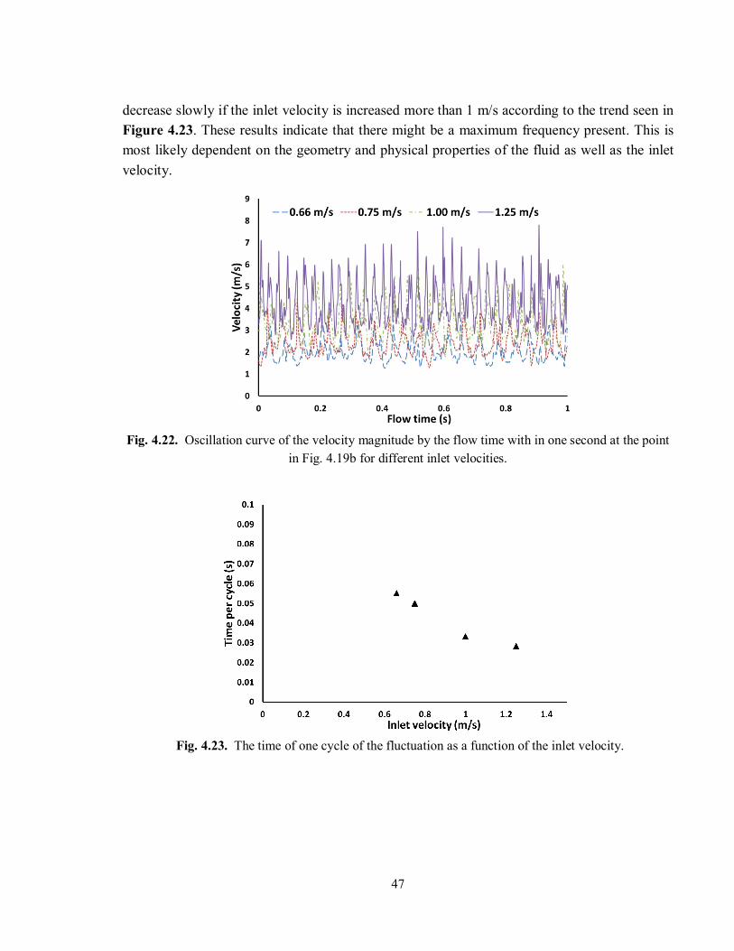
47

decrease slowly if the inlet velocity is increased more than 1 m/s according to the trend seen in Figure 4.23. These results indicate that there might be a maximum frequency present. This is most likely dependent on the geometry and physical properties of the fluid as well as the inlet velocity.

Fig. 4.22. Oscillation curve of the velocity magnitude by the flow time with in one second at the point

in Fig. 4.19b for different inlet velocities.

Fig. 4.23. The time of one cycle of the fluctuation as a function of the inlet velocity.

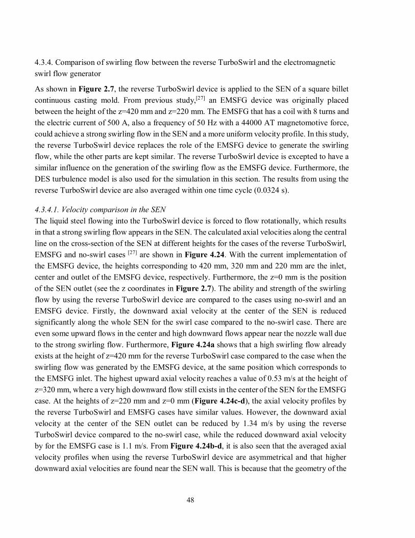
48

4.3.4. Comparison of swirling flow between the reverse TurboSwirl and the electromagnetic swirl flow generator

As shown in Figure 2.7, the reverse TurboSwirl device is applied to the SEN of a square billet continuous casting mold. From previous study,[27] an EMSFG device was originally placed between the height of the z=420 mm and z=220 mm. The EMSFG that has a coil with 8 turns and the electric current of 500 A, also a frequency of 50 Hz with a 44000 AT magnetomotive force, could achieve a strong swirling flow in the SEN and a more uniform velocity profile. In this study, the reverse TurboSwirl device replaces the role of the EMSFG device to generate the swirling flow, while the other parts are kept similar. The reverse TurboSwirl device is excepted to have a similar influence on the generation of the swirling flow as the EMSFG device. Furthermore, the DES turbulence model is also used for the simulation in this section. The results from using the reverse TurboSwirl device are also averaged within one time cycle (0.0324 s).

4.3.4.1. Velocity comparison in the SEN The liquid steel flowing into the TurboSwirl device is forced to flow rotationally, which results in that a strong swirling flow appears in the SEN. The calculated axial velocities along the central line on the cross-section of the SEN at different heights for the cases of the reverse TurboSwirl, EMSFG and no-swirl cases [27] are shown in Figure 4.24. With the current implementation of the EMSFG device, the heights corresponding to 420 mm, 320 mm and 220 mm are the inlet, center and outlet of the EMSFG device, respectively. Furthermore, the z=0 mm is the position of the SEN outlet (see the z coordinates in Figure 2.7). The ability and strength of the swirling flow by using the reverse TurboSwirl device are compared to the cases using no-swirl and an EMSFG device. Firstly, the downward axial velocity at the center of the SEN is reduced significantly along the whole SEN for the swirl case compared to the no-swirl case. There are even some upward flows in the center and high downward flows appear near the nozzle wall due to the strong swirling flow. Furthermore, Figure 4.24a shows that a high swirling flow already exists at the height of z=420 mm for the reverse TurboSwirl case compared to the case when the swirling flow was generated by the EMSFG device, at the same position which corresponds to the EMSFG inlet. The highest upward axial velocity reaches a value of 0.53 m/s at the height of z=320 mm, where a very high downward flow still exists in the center of the SEN for the EMSFG case. At the heights of z=220 mm and z=0 mm (Figure 4.24c-d), the axial velocity profiles by the reverse TurboSwirl and EMSFG cases have similar values. However, the downward axial velocity at the center of the SEN outlet can be reduced by 1.34 m/s by using the reverse TurboSwirl device compared to the no-swirl case, while the reduced downward axial velocity by for the EMSFG case is 1.1 m/s. From Figure 4.24b-d, it is also seen that the averaged axial velocity profiles when using the reverse TurboSwirl device are asymmetrical and that higher downward axial velocities are found near the SEN wall. This is because that the geometry of the

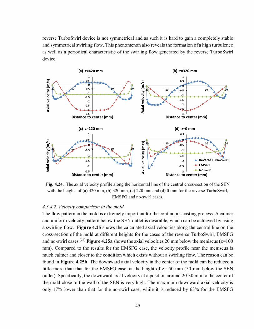
49

reverse TurboSwirl device is not symmetrical and as such it is hard to gain a completely stable and symmetrical swirling flow. This phenomenon also reveals the formation of a high turbulence as well as a periodical characteristic of the swirling flow generated by the reverse TurboSwirl device.

Fig. 4.24. The axial velocity profile along the horizontal line of the central cross-section of the SEN with the heights of (a) 420 mm, (b) 320 mm, (c) 220 mm and (d) 0 mm for the reverse TurboSwirl,

EMSFG and no-swirl cases.

4.3.4.2. Velocity comparison in the mold The flow pattern in the mold is extremely important for the continuous casting process. A calmer and uniform velocity pattern below the SEN outlet is desirable, which can be achieved by using a swirling flow. Figure 4.25 shows the calculated axial velocities along the central line on the cross-section of the mold at different heights for the cases of the reverse TurboSwirl, EMSFG

and no-swirl cases.[27] Figure 4.25a shows the axial velocities 20 mm below the meniscus (z=100 mm). Compared to the results for the EMSFG case, the velocity profile near the meniscus is much calmer and closer to the condition which exists without a swirling flow. The reason can be found in Figure 4.25b. The downward axial velocity in the center of the mold can be reduced a little more than that for the EMSFG case, at the height of z=-50 mm (50 mm below the SEN outlet). Specifically, the downward axial velocity at a position around 20-30 mm to the center of the mold close to the wall of the SEN is very high. The maximum downward axial velocity is only 17% lower than that for the no-swirl case, while it is reduced by 63% for the EMSFG

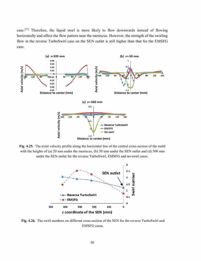
50

case.[27] Therefore, the liquid steel is more likely to flow downwards instead of flowing horizontally and affect the flow pattern near the meniscus. However, the strength of the swirling flow in the reverse TurboSwirl case on the SEN outlet is still higher than that for the EMSFG case.

Fig. 4.25. The axial velocity profile along the horizontal line of the central cross-section of the mold with the heights of (a) 20 mm under the meniscus, (b) 50 mm under the SEN outlet and (d) 500 mm

under the SEN outlet for the reverse TurboSwirl, EMSFG and no-swirl cases.

Fig. 4.26. The swirl numbers on different cross-section of the SEN for the reverse TurboSwirl and

EMSFG cases.

51

Figure 4.26 shows the calculated swirl numbers at the cross-section of the SEN. The swirl number is defined as Sw=2T/3U, where T and U are the average tangential and axial velocity on the specific cross-section of the SEN, respectively.[8] The swirl number at the SEN outlet by the reverse TurboSwirl gradually decreases from 2.09 to 1.24 at the upper part of the SEN. The swirl number for the EMSFG case sharply decreases from 2.54 to 0.77 at the SEN outlet after being accelerating by the EMSFG device. At a lower position of the mold of 500 mm below the SEN outlet in Figure 4.25c, it can be seen that the downward axial velocity profiles for the reverse TurboSwirl and EMSFG cases are both quite uniform compared to the no-swirl case. The asymmetry of the swirling flow by the reverse TurboSwirl can also be observed in Figure 4.25a-b.

4.4 Improvement by the divergent reverse TurboSwirl nozzle (DRTSN) in the continuous casting process

From the results in chapter 4.3 (Supplement III), it was also found that the fluid was more likely to flow downwards instead of flowing horizontally at the outlet of the SEN when using the reverse TurboSwirl design, which only had a slight influence on the removal of the inclusion to the meniscus. Therefore, a divergent nozzle was designed to replace the straight part at the end of the SEN, together with the reverse TurboSwirl connected on the top of the SEN. This nozzle was named a divergent reverse TurboSwirl nozzle (DRTSN). The swirling strength and the velocity fields are compared between the SRTSN and the DRTSN cases. A significant improvement was found when using the DRTSN compared to the SRTSN. The influence of the inlet velocity on the swirl strength was also studied. Furthermore, the distance between the elbow and the reverse TurboSwirl was investigated to obtain a better flow pattern in the mold.

4.4.1 The comparison of the SRTSN and the DRTSN

Compared to the straight nozzle at the end of the SEN, the divergent nozzle can make more liquid steel flow towards the wall of the mold. Furthermore, it can homogenise the flow field and the temperature field as well. The Figure 4.27 shows the streamlines of the liquid steel in the SEN and mold for the SRTSM and DRTSN cases. The liquid steel flowing out from the SRTSN are more intensive compared to the flow pattern by the DRTSN in the mold. More specifically, there are more circulation flows in the mold when using the SRTSN. Furthermore, some of them even appear in the low part of the mold where a strong turbulence could result in an unstable flow pattern. The flow pattern in the mold by the DRTSN device is more smooth and stable. Furthermore, the velocity fluctuation over the flow time are plotted at two points after the flow field has stabilized during the transient simulation.

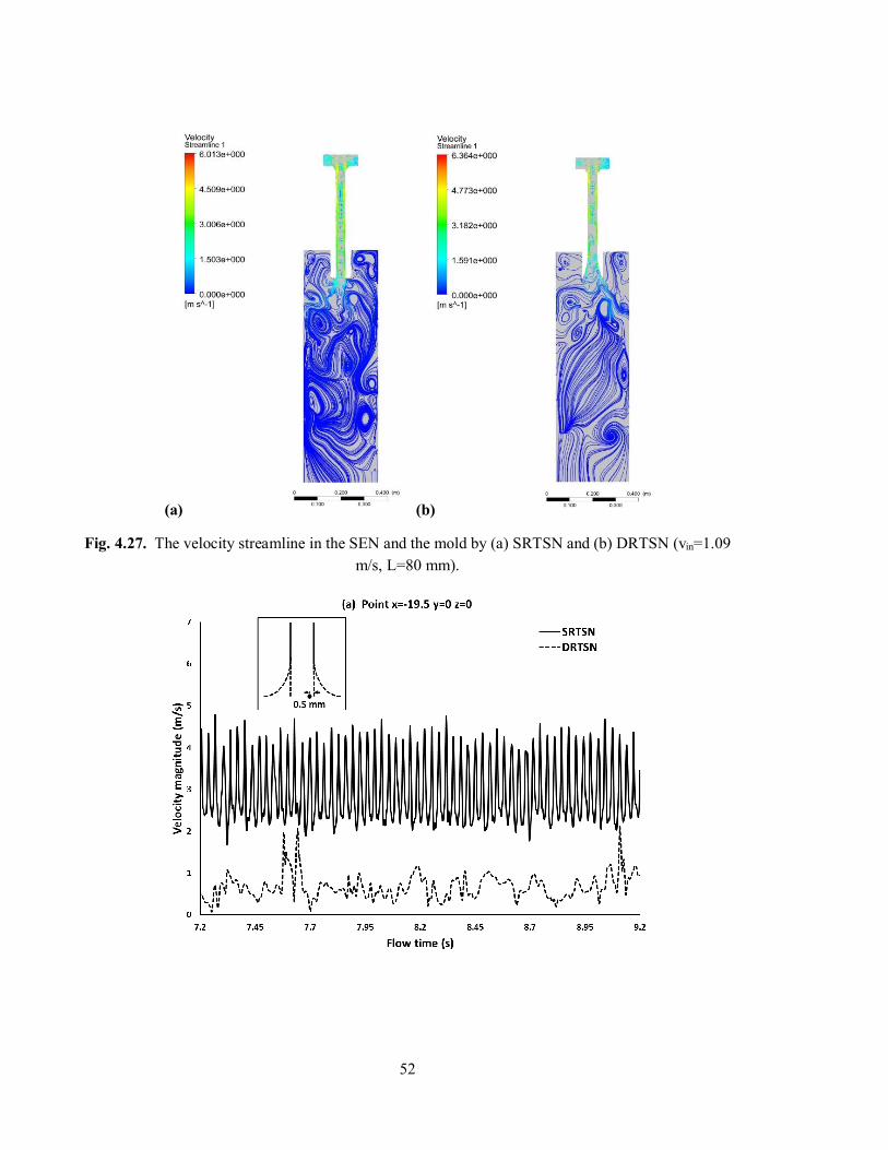
52

(a) (b)

Fig. 4.27. The velocity streamline in the SEN and the mold by (a) SRTSN and (b) DRTSN (vin=1.09 m/s, L=80 mm).

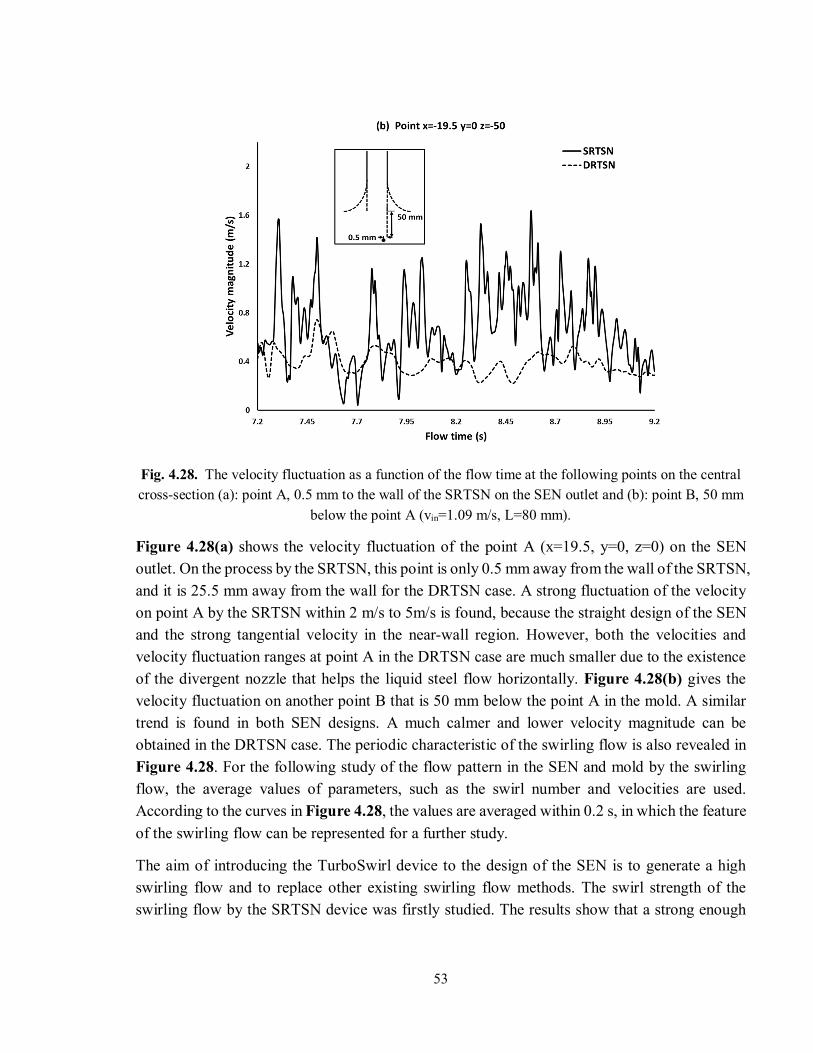
53

Fig. 4.28. The velocity fluctuation as a function of the flow time at the following points on the central cross-section (a): point A, 0.5 mm to the wall of the SRTSN on the SEN outlet and (b): point B, 50 mm

below the point A (vin=1.09 m/s, L=80 mm).

Figure 4.28(a) shows the velocity fluctuation of the point A (x=19.5, y=0, z=0) on the SEN outlet. On the process by the SRTSN, this point is only 0.5 mm away from the wall of the SRTSN, and it is 25.5 mm away from the wall for the DRTSN case. A strong fluctuation of the velocity on point A by the SRTSN within 2 m/s to 5m/s is found, because the straight design of the SEN and the strong tangential velocity in the near-wall region. However, both the velocities and velocity fluctuation ranges at point A in the DRTSN case are much smaller due to the existence of the divergent nozzle that helps the liquid steel flow horizontally. Figure 4.28(b) gives the velocity fluctuation on another point B that is 50 mm below the point A in the mold. A similar trend is found in both SEN designs. A much calmer and lower velocity magnitude can be obtained in the DRTSN case. The periodic characteristic of the swirling flow is also revealed in Figure 4.28. For the following study of the flow pattern in the SEN and mold by the swirling flow, the average values of parameters, such as the swirl number and velocities are used. According to the curves in Figure 4.28, the values are averaged within 0.2 s, in which the feature of the swirling flow can be represented for a further study.

The aim of introducing the TurboSwirl device to the design of the SEN is to generate a high swirling flow and to replace other existing swirling flow methods. The swirl strength of the swirling flow by the SRTSN device was firstly studied. The results show that a strong enough

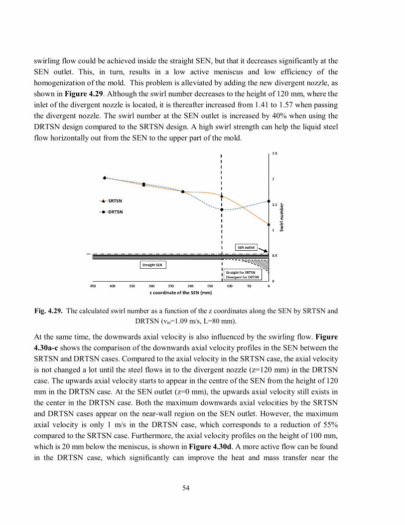
54

swirling flow could be achieved inside the straight SEN, but that it decreases significantly at the SEN outlet. This, in turn, results in a low active meniscus and low efficiency of the homogenization of the mold. This problem is alleviated by adding the new divergent nozzle, as shown in Figure 4.29. Although the swirl number decreases to the height of 120 mm, where the inlet of the divergent nozzle is located, it is thereafter increased from 1.41 to 1.57 when passing the divergent nozzle. The swirl number at the SEN outlet is increased by 40% when using the DRTSN design compared to the SRTSN design. A high swirl strength can help the liquid steel flow horizontally out from the SEN to the upper part of the mold.

Fig. 4.29. The calculated swirl number as a function of the z coordinates along the SEN by SRTSN and DRTSN (vin=1.09 m/s, L=80 mm).

At the same time, the downwards axial velocity is also influenced by the swirling flow. Figure 4.30a-c shows the comparison of the downwards axial velocity profiles in the SEN between the SRTSN and DRTSN cases. Compared to the axial velocity in the SRTSN case, the axial velocity is not changed a lot until the steel flows in to the divergent nozzle (z=120 mm) in the DRTSN case. The upwards axial velocity starts to appear in the centre of the SEN from the height of 120 mm in the DRTSN case. At the SEN outlet (z=0 mm), the upwards axial velocity still exists in the center in the DRTSN case. Both the maximum downwards axial velocities by the SRTSN and DRTSN cases appear on the near-wall region on the SEN outlet. However, the maximum axial velocity is only 1 m/s in the DRTSN case, which corresponds to a reduction of 55% compared to the SRTSN case. Furthermore, the axial velocity profiles on the height of 100 mm, which is 20 mm below the meniscus, is shown in Figure 4.30d. A more active flow can be found in the DRTSN case, which significantly can improve the heat and mass transfer near the

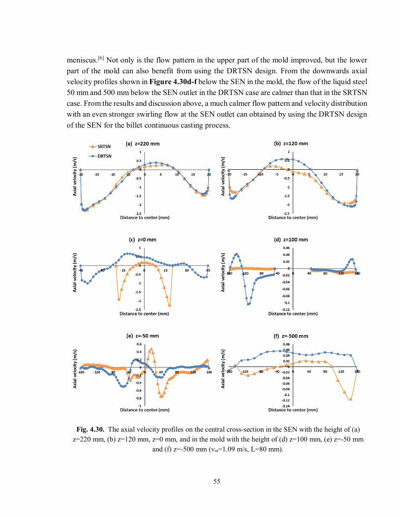
55

meniscus.[6] Not only is the flow pattern in the upper part of the mold improved, but the lower part of the mold can also benefit from using the DRTSN design. From the downwards axial velocity profiles shown in Figure 4.30d-f below the SEN in the mold, the flow of the liquid steel 50 mm and 500 mm below the SEN outlet in the DRTSN case are calmer than that in the SRTSN case. From the results and discussion above, a much calmer flow pattern and velocity distribution with an even stronger swirling flow at the SEN outlet can obtained by using the DRTSN design of the SEN for the billet continuous casting process.

Fig. 4.30. The axial velocity profiles on the central cross-section in the SEN with the height of (a) z=220 mm, (b) z=120 mm, z=0 mm, and in the mold with the height of (d) z=100 mm, (e) z=-50 mm

and (f) z=-500 mm (vin=1.09 m/s, L=80 mm).

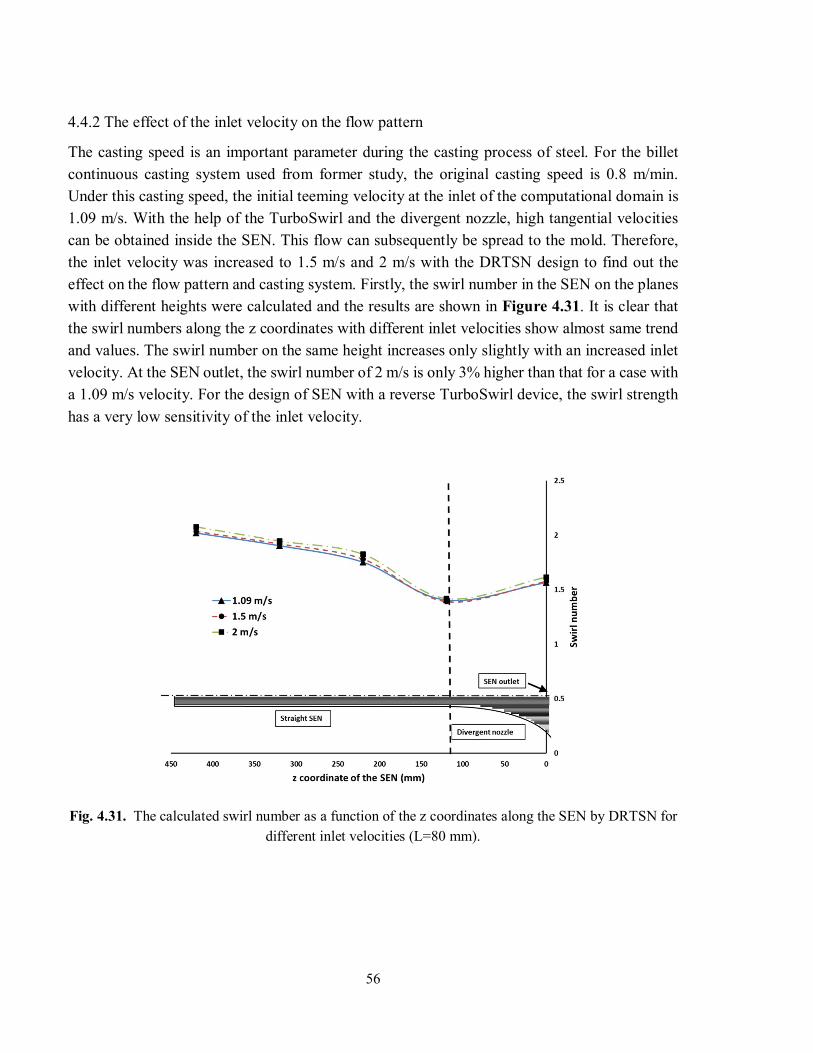
56

4.4.2 The effect of the inlet velocity on the flow pattern

The casting speed is an important parameter during the casting process of steel. For the billet continuous casting system used from former study, the original casting speed is 0.8 m/min. Under this casting speed, the initial teeming velocity at the inlet of the computational domain is 1.09 m/s. With the help of the TurboSwirl and the divergent nozzle, high tangential velocities can be obtained inside the SEN. This flow can subsequently be spread to the mold. Therefore, the inlet velocity was increased to 1.5 m/s and 2 m/s with the DRTSN design to find out the effect on the flow pattern and casting system. Firstly, the swirl number in the SEN on the planes with different heights were calculated and the results are shown in Figure 4.31. It is clear that the swirl numbers along the z coordinates with different inlet velocities show almost same trend and values. The swirl number on the same height increases only slightly with an increased inlet velocity. At the SEN outlet, the swirl number of 2 m/s is only 3% higher than that for a case with a 1.09 m/s velocity. For the design of SEN with a reverse TurboSwirl device, the swirl strength has a very low sensitivity of the inlet velocity.

Fig. 4.31. The calculated swirl number as a function of the z coordinates along the SEN by DRTSN for different inlet velocities (L=80 mm).

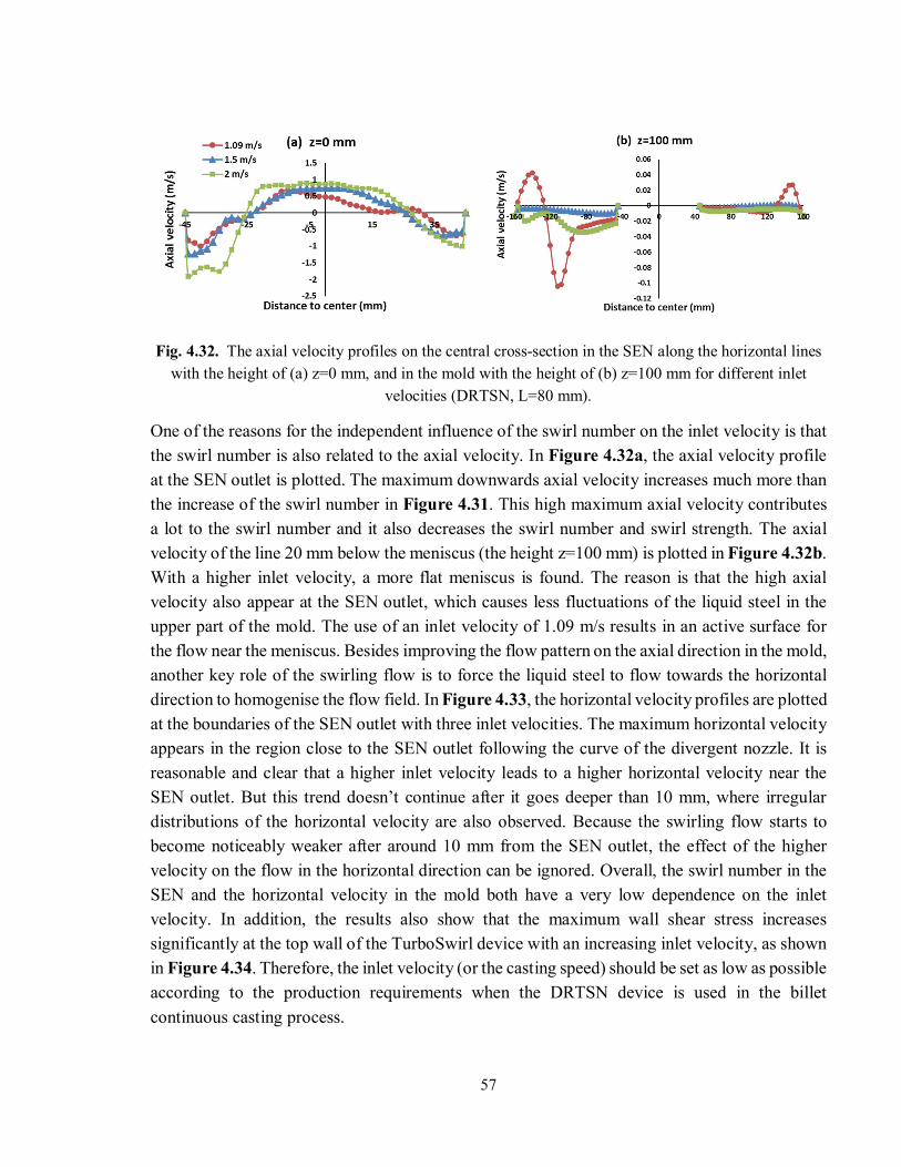
57

Fig. 4.32. The axial velocity profiles on the central cross-section in the SEN along the horizontal lines with the height of (a) z=0 mm, and in the mold with the height of (b) z=100 mm for different inlet

velocities (DRTSN, L=80 mm).

One of the reasons for the independent influence of the swirl number on the inlet velocity is that the swirl number is also related to the axial velocity. In Figure 4.32a, the axial velocity profile at the SEN outlet is plotted. The maximum downwards axial velocity increases much more than the increase of the swirl number in Figure 4.31. This high maximum axial velocity contributes a lot to the swirl number and it also decreases the swirl number and swirl strength. The axial velocity of the line 20 mm below the meniscus (the height z=100 mm) is plotted in Figure 4.32b. With a higher inlet velocity, a more flat meniscus is found. The reason is that the high axial velocity also appear at the SEN outlet, which causes less fluctuations of the liquid steel in the upper part of the mold. The use of an inlet velocity of 1.09 m/s results in an active surface for the flow near the meniscus. Besides improving the flow pattern on the axial direction in the mold, another key role of the swirling flow is to force the liquid steel to flow towards the horizontal direction to homogenise the flow field. In Figure 4.33, the horizontal velocity profiles are plotted at the boundaries of the SEN outlet with three inlet velocities. The maximum horizontal velocity appears in the region close to the SEN outlet following the curve of the divergent nozzle. It is reasonable and clear that a higher inlet velocity leads to a higher horizontal velocity near the SEN outlet. But this trend doesn’t continue after it goes deeper than 10 mm, where irregular distributions of the horizontal velocity are also observed. Because the swirling flow starts to become noticeably weaker after around 10 mm from the SEN outlet, the effect of the higher velocity on the flow in the horizontal direction can be ignored. Overall, the swirl number in the SEN and the horizontal velocity in the mold both have a very low dependence on the inlet velocity. In addition, the results also show that the maximum wall shear stress increases significantly at the top wall of the TurboSwirl device with an increasing inlet velocity, as shown in Figure 4.34. Therefore, the inlet velocity (or the casting speed) should be set as low as possible according to the production requirements when the DRTSN device is used in the billet continuous casting process.

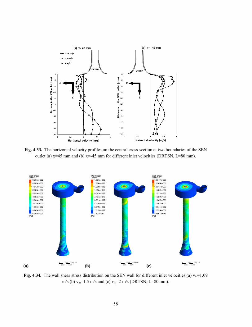
58

Fig. 4.33. The horizontal velocity profiles on the central cross-section at two boundaries of the SEN outlet (a) x=45 mm and (b) x=-45 mm for different inlet velocities (DRTSN, L=80 mm).

(a) (b) (c)

Fig. 4.34. The wall shear stress distribution on the SEN wall for different inlet velocities (a) vin=1.09 m/s (b) vin=1.5 m/s and (c) vin=2 m/s (DRTSN, L=80 mm).

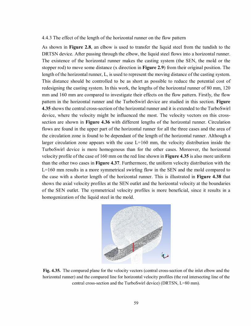
59

4.4.3 The effect of the length of the horizontal runner on the flow pattern

As shown in Figure 2.8, an elbow is used to transfer the liquid steel from the tundish to the DRTSN device. After passing through the elbow, the liquid steel flows into a horizontal runner. The existence of the horizontal runner makes the casting system (the SEN, the mold or the stopper rod) to move some distance (x direction in Figure 2.9) from their original position. The length of the horizontal runner, L, is used to represent the moving distance of the casting system. This distance should be controlled to be as short as possible to reduce the potential cost of redesigning the casting system. In this work, the lengths of the horizontal runner of 80 mm, 120 mm and 160 mm are compared to investigate their effects on the flow pattern. Firstly, the flow pattern in the horizontal runner and the TurboSwirl device are studied in this section. Figure 4.35 shows the central cross-section of the horizontal runner and it is extended to the TurboSwirl device, where the velocity might be influenced the most. The velocity vectors on this cross-section are shown in Figure 4.36 with different lengths of the horizontal runner. Circulation flows are found in the upper part of the horizontal runner for all the three cases and the area of the circulation zone is found to be dependant of the length of the horizontal runner. Although a larger circulation zone appears with the case L=160 mm, the velocity distribution inside the TurboSwirl device is more homogenous than for the other cases. Moreover, the horizontal velocity profile of the case of 160 mm on the red line shown in Figure 4.35 is also more uniform than the other two cases in Figure 4.37. Furthermore, the uniform velocity distribution with the L=160 mm results in a more symmetrical swirling flow in the SEN and the mold compared to the case with a shorter length of the horizontal runner. This is illustrated in Figure 4.38 that shows the axial velocity profiles at the SEN outlet and the horizontal velocity at the boundaries of the SEN outlet. The symmetrical velocity profiles is more beneficial, since it results in a homogenization of the liquid steel in the mold.

Fig. 4.35. The compared plane for the velocity vectors (central cross-section of the inlet elbow and the horizontal runner) and the compared line for horizontal velocity profiles (the red intersecting line of the

central cross-section and the TurboSwirl device) (DRTSN, L=80 mm).

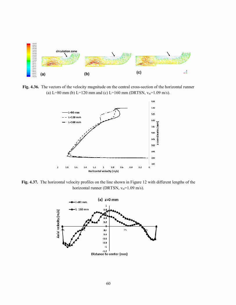
60

Fig. 4.36. The vectors of the velocity magnitude on the central cross-section of the horizontal runner (a) L=80 mm (b) L=120 mm and (c) L=160 mm (DRTSN, vin=1.09 m/s).

Fig. 4.37. The horizontal velocity profiles on the line shown in Figure 12 with different lengths of the horizontal runner (DRTSN, vin=1.09 m/s).

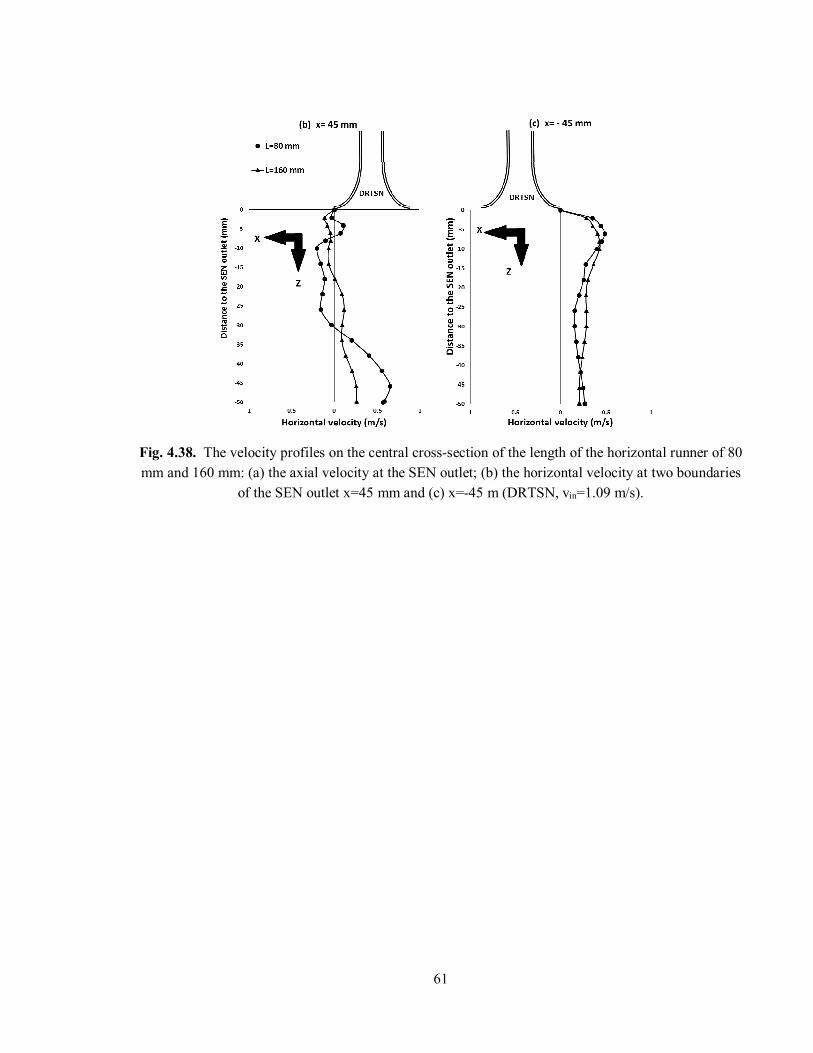
61

Fig. 4.38. The velocity profiles on the central cross-section of the length of the horizontal runner of 80 mm and 160 mm: (a) the axial velocity at the SEN outlet; (b) the horizontal velocity at two boundaries

of the SEN outlet x=45 mm and (c) x=-45 m (DRTSN, vin=1.09 m/s).

62

Chapter 5 Conclusion

The TurboSwirl device represents a simpler and probably a more economical alternative to the existing swirl technologies for generation of strong swirling flows in the casting process. In the thesis, the TurboSwirl device was applied to the casting process to generate a swirling flow that could achieve a beneficial flow pattern for the casting and solidification of the steel. In general, the implementation of the TurboSwirl device has been studied and investigated comprehensively with respect to the swirling flow pattern by the use of numerical simulations and water model experiments. The optimization and improvement have also been carried out with different aims and to obtain better designs. The results of this thesis complete the objectives set forth and represent a further increase of the knowledge due to the main following conclusions:

Optimization (Supplement I): The optimization of the TurboSwirl was done by investigating how structural factors influence the flow pattern of an uphill teeming ingot casting process. The flaring angle of the convergent nozzle and the position of the vertical runner were analysed, and the following main conclusions could were obtained:

(I.1) The flow pattern is remarkably influenced by the design of the divergent nozzle of the TurboSwirl device. A much more stable flow pattern can be achieved if a suitable flaring angle and a position of the convergent nozzle are selected; (I.2) A decrease of the flaring angle of the convergent nozzle can result in a lower maximum axial velocity both at the outlet and the entire domain. A lower or higher flaring angle causes a high maximum wall shear stress. With different flaring angles, the wall shear stress always has a great influence on the intensity of the swirling flow: a stronger rotation of a fluid induces a lower maximum wall shear stress, and a lower swirl number induces a higher maximum wall shear stress; Swirl numbers with flaring angles smaller than 60º result in larger differences that lead to higher intensities of the swirling flow; (I.3) The design of the TurboSwirl device can be adjusted according to the demand. If the need of decreasing the axial velocity is dominant in the teeming process, the convergent nozzle can be moved to zone II to achieve a lower maximum axial velocity, which leads to a calmer flow in the mold; If the vertical runner and the convergent nozzle are moved to a position far away from the centre of the TurboSwirl device, the refractory can be well protected from high wall shear stresses; The swirl number is higher when the vertical runner and the convergent nozzle are placed closer to the centre of the TurboSwirl device in Zone I.

63

Validation (Supplement II): A physical model of the novel TurboSwirl design for uphill teeming was built to validate the mathematical model to analyse the flow pattern inside the TurboSwirl device. The experiment confirms that the TurboSwirl design with a smaller flaring angle can create a strong swirling flow and a better flow pattern in the uphill teeming process. Overall, the following main conclusion were obtained:

(II.1) The swirling flow inside the TurboSwirl device was complex and an air-core vortex was intentionally formed in the vertical runner. The standard and realizable k-ɛ models were unable to simulate the formation of this vortex, but the Reynolds Stress Model could accurately simulate the vortex; (II.2) The radial velocity of the water around the vortex was measured by using the UVP method. A strong swirling flow and an instability of the vortex resulted in a high measured radial velocity fluctuation, so it was hard to obtain a stable radial velocity profile. However, the radial velocity at the upper part of the TurboSwirl generator could be simulated well with differences less than 5% compared to the measured values; (II.3) The shape and length of the vortex changed randomly and fluctuated within a limited range in the water model experiments; the length of air-core vortex could reflect the complex flow pattern inside the TurboSwirl device. Both the experimental and numerical results of the vortex length indicated that the vortex became longer with a smaller flaring angle of the divergent nozzle and if the swirl intensity was high. Also, a larger flaring angle caused a high maximum tangential velocity and a high wall shear stress, especially in the near wall region.

New implementation (Supplement III): A reverse TurboSwirl device was applied to the design of the SEN for the billet continuous casting process. Firstly, the water model experiment was carried out to validate the ability of the numerical simulation for this reverse TurboSwirl design. Afterwards, a SEN used in a square billet continuous casting operation was modified by this design and it was used to investigate the possibility to replace the original swirling flow generator by using the validated mathematical model. The main conclusions may be summarized as follows: (III.1) For the numerical simulation of the swirling flow by using the reverse TurboSwirl device, the DES turbulence model can more precisely predict the velocity distribution and the periodical characteristic compared to other turbulence models according to the measured results by the UVP instrument. The deviations of the DES averaged axial velocity to the measured velocity inside the vertical runner (SEN) were less than 3.1%; (III.2) The flow pattern inside the SEN shows some asymmetry and periodical characteristic due to the geometry of the TurboSwirl device. The periodical characteristic is dependent on the inlet velocity and should be highly considered if this design of a SEN is to be used in the future;

64

(III.3) The ability of generating a swirling flow by using the reverse TurboSwirl device was compared to the electromagnetic swirl flow generator (EMSFG) for a square billet continuous casting process. The results show that the design of the SEN by the reverse TurboSwirl device can provide an almost equivalent strength of the swirling flow generated by the EMSFG device with a 44000 AT magnetomotive force. It can also reduce more downward axial velocity in the center of the SEN outlet compared to that produced by the EMSFG device. Also, a more calm meniscus and internal flow of the mold can be found when using the TurboSwirl device compared to when using the EMSFG device.

Improvement (Supplement IV): The new design of the SEN was applied with the reverse TurboSwirl divergent nozzle (DRTSN) to replace the traditional SEN design and the straight nozzle. Based on a previous study, the computational fluid dynamic simulation was used to study the improvement of the DRTSN to the SRTSN designs. The effect of the inlet velocities on the swirl strength and flow pattern was also studied. Furthermore, the DRTSN device was implemented with an elbow to the tundish, and the length of the horizontal runner between the reverse TurboSwirl device and the elbow was investigated. The following main conclusions were found:

(IV.1) Compared to the straight reverse TurboSwirl nozzle, a divergent nozzle was added to the end of the SEN. The results show that swirl number was increased by 40% at the SEN outlet when using the DRTSN device compared to when using the SRTSN device. The enhanced swirling flow help the liquid steel to generate an active flow below the meniscus. The downwards axial velocity was also reduced by the divergent nozzle to form a calmer flow in the mold; (IV.2) The effect of the casting speed on the DRTSN device was also studied by changing the inlet velocity of the computational domain. The results show that the swirl strength has a very low sensitivity to the inlet velocity. However, the obvious downwards increase of the axial velocity at the nozzle outlet and maximum wall shear stress on the wall of the TurboSwirl device can be found with a higher casting speed; (IV.3) The problem of implementing the DRTSN device to the casting system is solved by implementing an elbow and a horizontal runner. A more uniform velocity distribution can be gained in the horizontal runner and in the reverse TurboSwirl device with a longer horizontal runner. The longer horizontal runner can also make the flow pattern more symmetrical to help to homogenise the liquid steel in the mold.

65

Chapter 6 Future Work

The swirling flow generated by the TurboSwirl device has been investigated with a focus on the flow pattern and velocity fields. According to the current progress, the future work can be continued in the following four directions:

(1) The asymmetry of the swirling flow has been improved to a certain extent, but further improvement needs to be done to gain a more even flow pattern. This includes the development of a symmetrical design of the TurboSwirl device and similar devices;

(2) Multiphase and multiphysics flow need to be investigated to better understand the behaviour of the molten flow in the SEN and the mold. For example, the slag can be added to the model to find out the effect of the swirling flow on the meniscus and the homogenization of the temperature field;

(3) The inclusion behaviour can be further studied with the optimized structure and using the new design of the SEN in the continuous casting process.

(4) Plant trials of the TurboSwirl device can be carried out to find out the availability of this new swirling flow generation device in the steel production.

66

References

[1] J. Campbell: Complete Casting Handbook: Metal Casting Processes, Metallurgy, Techniques and Design. Elsevier Ltd, 2011, 605-606.

[2] S. Yokoya, Y. Asako, S. Hara and J. Szekely: ISIJ Int., 1994, vol. 34, no. 11, pp. 883-888.

[3] L. Zhang, B. Rietow, B. G. Thomas and K. Eakin: ISIJ Int., 2006, vol. 46, no. 5, pp. 670-679.

[4] V. Singh, A. R. PAL, and P. Panigrahi: ISIJ Int., 2008, vol. 48, no. 4, pp. 430-437.

[5] S. Yokoya, R. Westoff, Y. Asako, S. Hara and J. Szekely: ISIJ Int., 1994, vol. 34, no. 11, pp. 889-895.

[6] S. Yokoya, S. Takagi, M. Iguchi, Y. Asako, R. Westoff and S. Hara: ISIJ Int., 1998, vol. 38, no. 8, pp. 827-833.

[7] S. Yokoya, S. Takagi, M. Iguchi, K, Marukawa and S. Hara: ISIJ Int., 2000, vol. 40, no. 6, pp. 578-583.

[8] S. Yokoya, S. Takagi, M. Iguchi, K. Marukawa, W. Yasugaria and S. Hara: ISIJ Int., 2000, vol. 40, no. 6, pp. 584-588.

[9] S. Yokoya, S. Takagi, K. Tada, M. Iguchi, K. Marukawa and S. Hara: ISIJ Int., 2001, vol. 41, no. 10, pp. 1201-1207.

[10] S. Yokoya, S. Takagi, S. Ootani, M. Iguchi, K. Marukawa and S. Hara: ISIJ Int., 2001, vol. 41, no. 10, pp. 1208-1214.

[11] S. Yokoya, S. Takagi, M. Kaneko, M. Iguchi, K. Marukawa and S. Hara: ISIJ Int., 2001, vol. 41, no. 10, pp. 1215-1220.

[12] S. Kholmatov, S. Takagi, L. Jonsson, P. Jönsson and S. Yokoya: ISIJ Int., 2007, vol. 47, no.1, pp. 80-87.

[13] G. Solorio-Diaz, R. D. Morales, J. Palafax-Ramos, L. Garcia-Demedices and A. Ramos-Banderas: ISIJ Int., 2004, vol. 44, no. 6, pp. 1014-1032.

[14] G. Solorio-Diaz, R. D. Morales and A. Ramos-Banderas: Int. J. Heat Mass Tran., 2005, vol. 48, pp. 3574-3590.

67

[15] G. Solorio-Diaz, R. D. Morales, J. Palafax-Ramos and A. Ramos-Banderas: ISIJ Int., 2005, vol. 45, no. 8, pp. 1129-1137.

[16] G. Solorio-Diaz, R. Davlia-Morales, J. Barreto-Sandoval, H. J. Vergara-Hernandez, A. Ramos-Banderas and S. R. Galvan: Steel Res. Int., 2014, vol. 85, no. 5, pp. 863-874.

[17] Y. Tsukaguchi, H. Hayashi, H. Kurimoto, S. Yokoya, K. Marukawa and T. Tanaka: ISIJ Int., 2010, vol. 50, no. 5, pp. 721-729.

[18] Y. Wang, Y. Zhong, B. Wang, Z. Lei, W. Ren and Z. Ren: ISIJ Int., 2009, vol. 49, no. 10, pp. 1542-1550.

[19] Q. Hou and Z. Zou: ISIJ Int., 2005, vol. 45, no. 3, pp. 325-330.

[20] Q. Hou, Q. Yue, H. Wang, Z. Zou and A. Yu: ISIJ Int., 2008, vol. 48, no. 6, pp. 787-792.

[21] P. Ni, L. T. I. Jonsson, M. Ersson and P. G. Jönsson: Steel Res. Int., 2016, vol. 87, no. 10, pp. 1356-1365.

[22] P. Ni, L. T. I. Jonsson, M. Ersson and P. G. Jönsson: Steel Res. Int., 2016, vol. 87, no. 9999, pp. 1-11.

[23] D. Li, Z. Su, L. Sun, K. Marukawa and J. He: Adv. Mat. Res., 2011, vol. 295-297, pp. 1284-1288.

[24] D. Li, Z. Su, J, Chen, Q. Wang, Y. Yang, K. Nakajima, K. Marukawa and J. He: ISIJ Int., 2013, vol. 53, no. 7, pp. 1187-1194.

[25] Y. Yang, P.G. Jönsson, Z. Su, J, He and K. Nakajima: Steel Res. Int., 2015, vol. 86, no. 4, pp. 361-374.

[26] B. Ren, M. Zhu, H. Wang and Y. Chen: Acta Metall. Sin., 2008, vol. 44, no. 4, pp. 507-512.

[27] Y. Yang, P. G. Jönsson, M. Ersson and K. Nakajima: Steel Res. Int., 2015, vol. 86, no. 4, pp. 341-360.

[28] L. Zhang anf B. G. Thomas: Metall. Mater. Trans. B, 2015, vol. 37B, no. 5, pp. 733-761.

[29] D. J. Hurtuk: ASM Int., 2008, vol. 15, pp. 911-917.

[30] R. Eriksson, P. Jönsson and A. Gustafsson: Scand. J. Metall., 2004, vol. 33, pp. 160-171.

[31] R. Eriksson, L. Jonsson, and P.G. Jönsson: ISIJ Int., 2004, vol. 44, no. 8, pp. 1358-1365.

[32] Z. Tan, M. Ersson and P.G. Jönsson: ISIJ Int., 2011, vol. 51, no. 9, pp. 1461-1467.

68

[33] L. Hallgren, S. Takagi, R. Eriksson, S. Yokoya and P.G. Jönsson: ISIJ Int., 2006, vol. 46, no. 11, pp. 1645-1651.

[34] L. Hallgren, S. Takagi, A. Tilliander, S. Yokoya and P.G. Jönsson: Steel Res. Int., 2007, vol. 78, no. 3, pp. 254-259.

[35] Z. Zhang, S. Yokoya, A. Tilliander and P. G. Jönsson: ISIJ Int., 2010, vol. 50, no. 12, pp. 1756-1762.

[36] L. Hallgren, A. Tilliander, S. Yokoya, P.G. Jönsson and S. Hagman: ISIJ Int., 2010, vol. 50, no. 12, pp. 1763-1769.

[37] Z. Tan, M. Ersson and P.G. Jönsson: ISIJ Int., 2012, vol. 52, no. 6, pp. 1066-1071.

[38] Z. Tan, M. Ersson and P.G. Jönsson: Technical Report TO24-183, Jernkontoret, 2012.

[39] Z. Tan, M. Ersson, P. Lidegran and P.G. Jönsson: Steel Res. Int., 2013, vol. 84, no. 9, pp. 837-844.

[40] G. Brüstlein, Eingußstein für das Gießen von Blöcken von unten, Kaiserliches Patentamt Number 285999, 1914.

[41] D. Hrabina, W. Janosik, P. Filp: Fond-FR, 2013, no.3, pp. 19-24.

[42] F. Y. Hsu, M. R. Jolly and J. Campbell: Int. J Cast Metal Res., 2006, vol. 19, no. 1, pp. 38-44.

[43] Z. Tan, M. Ersson and P.G. Jönsson: Math. Probl. Eng., 2015, vol. 2015, pp. 1-10.

[44] L. Nastac, L. Zhang, B. G. Thomas, M. Zhu, A. Ludwig, A. S. Sabau, K. Pericleous and H. Combeau: CFD Modeling and Simulation in Materials Processing. 2016, published by John Wiley & Sons, Inc., Hoboken, New Jersey, US.

[45] P. Gittler, R. Kickinger, S. Pirker, E. Fuhrmann, J. Lehner and J. Steins: Scand. J. Metall., 2000, vol. 29, no. 4, pp. 166-176.

[46] L. J. Mittoni and M. P. Schwarz: 13th Australasian Fluid Mechanics Conference, 1998, pp. 671-674.

[47] O. Reynolds: T. Roy. Soc. A, 1895, vol. 186, pp. 123-164.

[48] B. E. Launder and D. B. Spalding: Comput. Method Appl. M., 1974, vol. 3, pp. 269-289.

[49] D. M. Driver and H. L. Seegmiller: AIAA J., 1985, vol. 23, no. 2, pp. 163-171.

69

[50] T.-H. Shin, W. W. Liou, A. Shabbir, Z. Yang, and J. Zhu: Comput. Fluids, 1995, vol. 24, no. 3, pp. 227-238.

[51] A.J. Hoekstra, J.J. Derksen and H.E.A. Van Den Akker: Chem. Eng. Sci., 1999, vol. 54, pp. 2055-2065.

[52] B. E. Launder, G. J. Reece, and W. Rodi: J. Fluid Mech., 1975, vol. 68, no. 3, pp. 537-566.

[53] H. K. Versteeg and W. Malalasekera: An Introduction to Computational Fluid Dynamics: The Finite Volume Method, 2nd edition, Pearson Education Limited, Essex, 2007, pp. 75-92.

[54] ANSYS® Fluent Academic Research, Release 16.2, Help System, 4.9.2. Reynolds Stress Transport Equations, ANSYS, Inc.

[55] ANSYS® Fluent Academic Research, Release 14.5, Help System, 4.8.4.4. Low-Re Stress-Omega Model, ANSYS, Inc.

[56] ANSYS® Fluent Academic Research, Release 16.2, Help System, 4.11.1. Detached Eddy Simulation Overview, ANSYS, Inc.

[57] F. R. Menter: AIAA J., 1994, vol. 32, no. 8, pp. 1598–1605.

[58] F. R. Menter, M. Kuntz and R. Langtry: Turbulence, Heat and Mass Transfer 4, Eds: K. Hanjalic, Y. Nagano, and M. Tummers, Begell House Inc., 2003, pp. 625-632.

[59] P. R. Spalart, S. Deck, M. L. Shur, K. D. Squires, M. Kh. Strelets and A. Travin: Theor. Comp. Fluid Dyn., 2006, vol. 20, pp. 181-195.

[60] C. W. Hirt and B. D. Nichols: J. Comput. Phys., 1981, vol. 39, pp. 201-225.

[61] X. Huang and B. G. Thomas: Can. Metal. Quart., 1998, vol. 37, no. 3-4, pp.197-212.

[62] ANSYS® Fluent Academic Research, Release 16.2, Help System, 35.5.2. Fluent Database Materials Dialog Box, ANSYS, Inc.

[63] COMSOL Multiphysics® v. 4.4. www.comsol.com. COMSOL AB, Stockholm, Sweden.

[64] ANSYS® Fluent Academic Research, Release 14.5.

[65] ANSYS® Fluent Academic Research, Release 16.2.

[66] I. Celik, U. Ghia, P. J. Roache, C. J. Freitas, H. Coleman and P. E. Raad: J. Fluid Eng.-T. ASME, 2008, vol. 130, no. 7, pp. 078001-1-078011-4.

[67] X.K. Lan, J.M. Khodadadi and F. Shen: Metall. Mater. Trans. B, 1997, vol. 28, no. 2, pp. 321-332.

70

[68] Y. Takeda: Int. J. Heat & Fluid Flow, 1986, vol. 7, no. 4, pp. 313-318.

[69] Y. Takeda: Exp. Therm. Fluid Sci., 1995, vol. 10, no. 4, pp. 444-453.

[70] Ultrasound velocity profiler UVP-DUO user’s guide, Released 5.2, March 2014, Met-Flow SA, Chemin Auguste-Pidou 8, CH-1007 Lausanne, Switzerland.

[71] O. Kitoh: J. Fluid Mech., 1991, vol. 225, pp. 445-479.

[72] H. J. Sheen, W. J. Chen, S. Y. Jeng and T. L. Huang: Exp. Therm. Fluid Sci., 1996, vol. 12, no. 4, pp. 444-451.

[73] W. J. M. Rankine: A Manual of Applied Mechanics, C. Griffen Co., London, England, 1858, pp. 576.

[74] J. E. Hite Jr., W. C. Mih: J. Hydraul. Eng-ASCE, 1994, vol. 120, no. 3, pp. 284-297.

[75] T. J. Bennett: Ph.D. thesis, Washington State University, 1988.

[76] W. C. Mih.: J. Hydraul. Res., 1990, vol. 28, no. 3, pp. 392-396.

[77] P. Ni, L. T. Jonsson, M. Ersson and P.G. Jönsson: Int. J. Multiphas. Flow, 2014, vol. 62, pp. 152-160.