A Study of the Piston Cylinder Interface of Axial Piston Machines

Purdue University Purdue University

Purdue e-Pubs Purdue e-Pubs

Open Access Dissertations Theses and Dissertations

5-2018

A Study of the Piston Cylinder Interface of Axial Piston Machines A Study of the Piston Cylinder Interface of Axial Piston Machines

Daniel Mizell Purdue University

Follow this and additional works at: https://docs.lib.purdue.edu/open_access_dissertations

Recommended Citation Recommended Citation Mizell, Daniel, "A Study of the Piston Cylinder Interface of Axial Piston Machines" (2018). Open Access Dissertations. 1876. https://docs.lib.purdue.edu/open_access_dissertations/1876

This document has been made available through Purdue e-Pubs, a service of the Purdue University Libraries. Please contact [email protected] for additional information.

https://docs.lib.purdue.edu/

https://docs.lib.purdue.edu/open_access_dissertations

https://docs.lib.purdue.edu/etd

https://docs.lib.purdue.edu/open_access_dissertations?utm_source=docs.lib.purdue.edu%2Fopen_access_dissertations%2F1876&utm_medium=PDF&utm_campaign=PDFCoverPages

https://docs.lib.purdue.edu/open_access_dissertations/1876?utm_source=docs.lib.purdue.edu%2Fopen_access_dissertations%2F1876&utm_medium=PDF&utm_campaign=PDFCoverPages

A STUDY OF THE PISTON CYLINDER INTERFACE OF AXIAL PISTON

MACHINES

A Dissertation

Submitted to the Faculty

of

Purdue University

by

Daniel Mizell

In Partial Fulfillment of the

Requirements for the Degree

of

Doctor of Philosophy

May 2018

Purdue University

West Lafayette, Indiana

THE PURDUE UNIVERSITY GRADUATE SCHOOL

STATEMENT OF COMMITTEE APPROVAL

Dr. Monika Ivantysynova, Chair

Department of Agricultural and Biological Engineering

Dr. Andrea Vacca

Department of Agricultural and Biological Engineering

Dr. Farshid Sadeghi

Department of Mechanical Engineering

Dr. Karthik Ramani

Department of Mechanical Engineering

Approved by:

Dr. Jay P. Gore

Head of the Graduate Program

ii

To my wife Ashby and son Troy, my refuge and inspiration.

iii

ACKNOWLEDGMENTS

I would like to first thank Dr. Ivantysynova for offering me the opportunity to be

a part of the Maha Fluid Power Research Center team. Her guidance and example

have been an invaluable influence and inspiration to me and my research. Through

my circuitous journey of discovery her advice and encouragement have been unfailing.

I also need to thank my many coworkers at the Maha lab. Each and every one

has contributed in some way to the wonderful experience I have had. Special thanks

to Matteo Pelosi whose PhD work formed my starting point, and to Andrew Schenk

whose extensive tutoring enables me to use and maintain the Maha computer network.

Thanks also to the pump modeling group, particularly Lizhi Shang, Ashley Busquets

(Wondergem), and Meike Ernst for their help in testing the model, discussion, and

suggestions. Thanks as well to all those who assisted me with the Tribo test rig,

especially Anthony Franklin, Anna Garcia Teruel, and Cory Raizor. Finally, a special

thanks to Susan Gauger and Connie McMindes who do so much to brighten the lives

of the Maha family.

Most of all I must thank my family for their support and encouragement through-

out. Thanks to my wife Ashby for encouraging me to make the most of this oppor-

tunity, and for her constant love and support throughout my studies. Thanks to my

parents and parents-in-law for their support and guidance. You have all made this

possible.

iv

TABLE OF CONTENTS

Page

LIST OF TABLES . . . . . . . . . . . . . . . . . . . . . . . . . . . . . . . . . . vi

LIST OF FIGURES . . . . . . . . . . . . . . . . . . . . . . . . . . . . . . . . . vii

SYMBOLS . . . . . . . . . . . . . . . . . . . . . . . . . . . . . . . . . . . . . . xi

ABSTRACT . . . . . . . . . . . . . . . . . . . . . . . . . . . . . . . . . . . . . xv

1. INTRODUCTION . . . . . . . . . . . . . . . . . . . . . . . . . . . . . . . . 1

2. STATE OF THE ART . . . . . . . . . . . . . . . . . . . . . . . . . . . . . . 32.1 Modeling of the Piston Cylinder Interface . . . . . . . . . . . . . . . . . 3

2.1.1 Piston Dynamics . . . . . . . . . . . . . . . . . . . . . . . . . . 52.1.2 Calculating Fluid Pressure Build Up . . . . . . . . . . . . . . . 72.1.3 Surface Wear Profiles . . . . . . . . . . . . . . . . . . . . . . . . 72.1.4 Force Balance . . . . . . . . . . . . . . . . . . . . . . . . . . . . 8

2.2 Experimental Investigation of the Piston Cylinder Interface . . . . . . . 152.3 Modeling of Tribological Point and Line Contacts . . . . . . . . . . . . 202.4 Research Goals . . . . . . . . . . . . . . . . . . . . . . . . . . . . . . . 21

3. THE NOVEL PISTON CYLINDER INTERFACE MODEL . . . . . . . . . 233.1 Pressure Field Model and Calculation . . . . . . . . . . . . . . . . . . . 243.2 Surface Wear Profiles . . . . . . . . . . . . . . . . . . . . . . . . . . . . 26

3.2.1 The Fluid Grid . . . . . . . . . . . . . . . . . . . . . . . . . . . 303.3 Solid Body Temperature Distribution . . . . . . . . . . . . . . . . . . . 333.4 Solid Body Pressure Deformation . . . . . . . . . . . . . . . . . . . . . 333.5 Preventing Fluid Film Collapse . . . . . . . . . . . . . . . . . . . . . . 36

3.5.1 Linear Method . . . . . . . . . . . . . . . . . . . . . . . . . . . 383.5.2 Iterative Method . . . . . . . . . . . . . . . . . . . . . . . . . . 40

4. SIMULATION RESULTS AND MEASUREMENT COMPARISON . . . . . 424.1 The Tribo Test Rig . . . . . . . . . . . . . . . . . . . . . . . . . . . . . 424.2 Tribo Test Rig Data Processing . . . . . . . . . . . . . . . . . . . . . . 444.3 Measured Operating Conditions . . . . . . . . . . . . . . . . . . . . . . 48

4.3.1 500rpm 80bar . . . . . . . . . . . . . . . . . . . . . . . . . . . . 484.3.2 500rpm 120bar . . . . . . . . . . . . . . . . . . . . . . . . . . . 53

v

Page4.3.3 500rpm 150bar . . . . . . . . . . . . . . . . . . . . . . . . . . . 574.3.4 500rpm 190bar . . . . . . . . . . . . . . . . . . . . . . . . . . . 59

4.4 Evaluating the Models . . . . . . . . . . . . . . . . . . . . . . . . . . . 61

5. THE HIGH DEFINITION LUBRICATION MODEL . . . . . . . . . . . . . 625.1 Modeling Approach . . . . . . . . . . . . . . . . . . . . . . . . . . . . . 63

5.1.1 Generation of Inputs . . . . . . . . . . . . . . . . . . . . . . . . 635.1.2 Surface Pressure Deformation . . . . . . . . . . . . . . . . . . . 685.1.3 Adaptive Grid Refinement . . . . . . . . . . . . . . . . . . . . . 725.1.4 Fluid Properties . . . . . . . . . . . . . . . . . . . . . . . . . . . 725.1.5 Pressure Build Up . . . . . . . . . . . . . . . . . . . . . . . . . 735.1.6 Result Compilation . . . . . . . . . . . . . . . . . . . . . . . . . 74

6. INTEGRATING HD PRESSURE CALCULATIONS WITH THE PISTONCYLINDER MODEL . . . . . . . . . . . . . . . . . . . . . . . . . . . . . . . 776.1 Pressure Buildup Calculations . . . . . . . . . . . . . . . . . . . . . . . 776.2 Adaptive Mesh Refinement . . . . . . . . . . . . . . . . . . . . . . . . . 786.3 A New Force Balance Solver . . . . . . . . . . . . . . . . . . . . . . . . 79

7. HIGH DEFINITION PISTON CYLINDER SIMULATION RESULTS ANDMEASUREMENT COMPARISON . . . . . . . . . . . . . . . . . . . . . . . 807.1 Measurement Data Post-Processing . . . . . . . . . . . . . . . . . . . . 817.2 Simulation Comparison to Measurement . . . . . . . . . . . . . . . . . 83

7.2.1 Cylinder Surface Temperature . . . . . . . . . . . . . . . . . . . 837.2.2 Film Pressure . . . . . . . . . . . . . . . . . . . . . . . . . . . . 85

7.3 Comparison of Standard Piston Cylinder Model to HD Piston CylinderModel . . . . . . . . . . . . . . . . . . . . . . . . . . . . . . . . . . . . 907.3.1 Load Support . . . . . . . . . . . . . . . . . . . . . . . . . . . . 907.3.2 Friction Forces . . . . . . . . . . . . . . . . . . . . . . . . . . . 917.3.3 Energy Dissipation . . . . . . . . . . . . . . . . . . . . . . . . . 927.3.4 Leakage Flow . . . . . . . . . . . . . . . . . . . . . . . . . . . . 937.3.5 Piston Motion . . . . . . . . . . . . . . . . . . . . . . . . . . . . 947.3.6 Film Thickness . . . . . . . . . . . . . . . . . . . . . . . . . . . 95

8. CONTRIBUTIONS . . . . . . . . . . . . . . . . . . . . . . . . . . . . . . . . 98

LIST OF REFERENCES . . . . . . . . . . . . . . . . . . . . . . . . . . . . . 100

VITA . . . . . . . . . . . . . . . . . . . . . . . . . . . . . . . . . . . . . . . . 104

vi

LIST OF TABLES

Table Page

2.1 Tribo test rig operating condition. . . . . . . . . . . . . . . . . . . . . . . . 17

4.1 Operating condition information 500rpm 80bar. . . . . . . . . . . . . . . . 49

4.2 Operating condition information 500rpm 120bar. . . . . . . . . . . . . . . 53



7.1 EHD test rig operating condition. . . . . . . . . . . . . . . . . . . . . . . . 80

7.2 EHD pressure sensor model parameters. . . . . . . . . . . . . . . . . . . . 82

vii

LIST OF FIGURES

Figure Page

1.1 Lubricating interfaces of axial piston machines. . . . . . . . . . . . . . . . 2

2.1 Forces acting on the piston cylinder interface. . . . . . . . . . . . . . . . . 5

2.2 Measured displacement chamber pressure from Tribo test rig, 500rpm. . . 6

2.3 Force balance at the piston cylinder interface in the model developed byPelosi [15]. . . . . . . . . . . . . . . . . . . . . . . . . . . . . . . . . . . . . 11

2.4 Calculation of correction stress for velocity correction method. . . . . . . . 12

2.5 Piston position in the model developed by Pelosi [15]. . . . . . . . . . . . . 13

2.6 Area of collapsed film occurring with no correction forces calculated whenwear profiles are introduced. Correction stress only considered to the rightof green line. . . . . . . . . . . . . . . . . . . . . . . . . . . . . . . . . . . 14

2.7 Cross section view of Tribo test rig. . . . . . . . . . . . . . . . . . . . . . . 18

2.8 Sample Tribo test rig measurement compared to a simulation using themodel developed by Pelosi [15]. . . . . . . . . . . . . . . . . . . . . . . . . 19

2.9 Cross section view of EHD test rig. . . . . . . . . . . . . . . . . . . . . . . 19

3.1 Piston cylinder modeling approach. . . . . . . . . . . . . . . . . . . . . . . 24

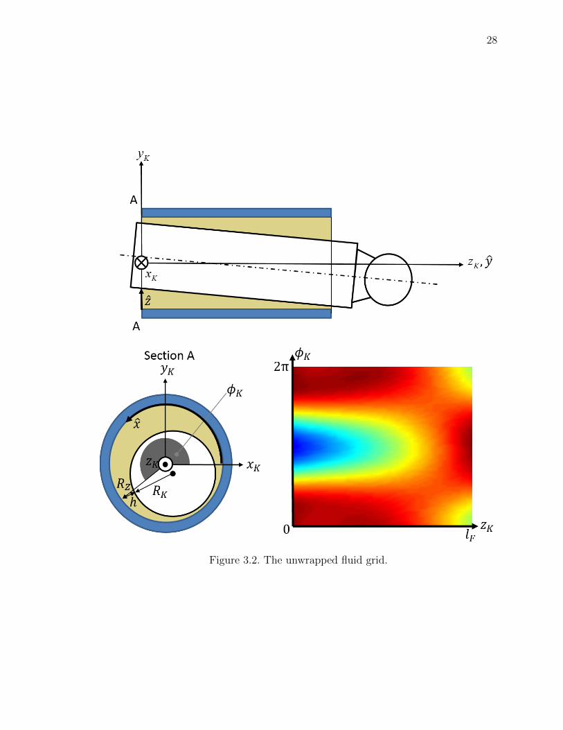
3.2 The unwrapped fluid grid. . . . . . . . . . . . . . . . . . . . . . . . . . . . 28

3.3 Experimental surface profile measurement of a bushing from the Tribo testrig. . . . . . . . . . . . . . . . . . . . . . . . . . . . . . . . . . . . . . . . . 29

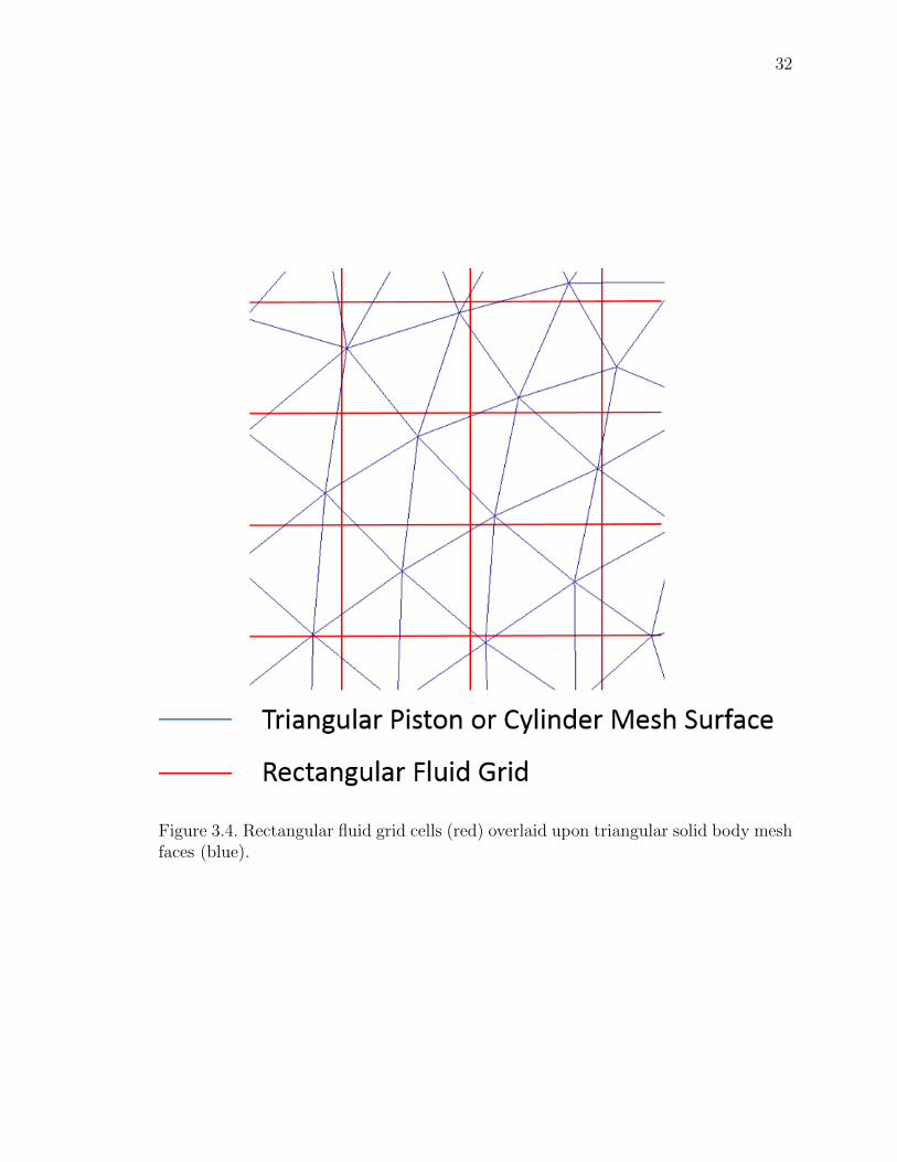
3.4 Rectangular fluid grid cells (red) overlaid upon triangular solid body meshfaces (blue). . . . . . . . . . . . . . . . . . . . . . . . . . . . . . . . . . . . 32

3.5 Cylinder block mesh showing face definitions for pressure loading. . . . . . 35

3.6 Force balance at the piston cylinder interface. . . . . . . . . . . . . . . . . 37

3.7 Calculation of linear force balance correction stress. . . . . . . . . . . . . . 39

3.8 Calculation of iterative force balance correction stress. . . . . . . . . . . . 41

viii

Figure Page

4.1 Hydraulic circuit for Tribo test rig. . . . . . . . . . . . . . . . . . . . . . . 43

4.2 Aligned telemetry signals from Tribo test rig displacement chamber pres-sure sensor. . . . . . . . . . . . . . . . . . . . . . . . . . . . . . . . . . . . 45

4.3 Aligned telemetry signals from Tribo test rig axial friction force sensor. . . 46

4.4 Creation of a histogram from a single shaft angle of multiple revolutions. . 47

4.5 Creation of a time-varying histogram contour from individual histograms. . 47

4.6 Modified wear profile for the bushing used in the presented measurements. 50

4.7 Simulated friction vs. measurement. Tribo test rig, 500rpm 80bar 42C.From top left: full code, without transient squeeze, with incompressibleReynolds, without translational squeeze, iterative force correction, velocitycorrection. . . . . . . . . . . . . . . . . . . . . . . . . . . . . . . . . . . . . 51

4.8 Simulated film thickness for full code (top) and change in film thicknessdue to iterative force correction (bottom). Tribo test rig, 500rpm 80bar 42C.52

4.9 Measured wear for the bushing used in the presented measurements. . . . . 54


4.11 Correction forces normalized to external forces for full model (top) andmodel with incompressible fluid (bottom). . . . . . . . . . . . . . . . . . . 56



5.1 Film thickness (contours), fluid pressure (blue shading), and correctionstress (red shading). . . . . . . . . . . . . . . . . . . . . . . . . . . . . . . 65

5.2 Regions of interest defined based on film thickness. . . . . . . . . . . . . . 66

5.3 Section of linear half space domain showing applied pressure in yellowrectangle centered at point (X1, Y1), and deformation calculated at point(X, Y ). . . . . . . . . . . . . . . . . . . . . . . . . . . . . . . . . . . . . . . 70

ix

Figure Page

5.4 Example of superposition of two rectangular areas of applied pressure onhalf space deformation model. . . . . . . . . . . . . . . . . . . . . . . . . . 70

5.5 Pressures applied to deformation model in refined areas. . . . . . . . . . . 71

5.6 Sample HD analysis output for single analysis region. Color indicatesfluid pressure in bar, contours indicate film thickness in µm. . . . . . . . . 75

5.7 Sample HD analysis cumulative output. Circle size indicates required loadsupport. Tribo Test Rig, 500rpm, 120bar. . . . . . . . . . . . . . . . . . . 76

6.1 Nonuniformity of film thickness Uh in one dimensional grid. . . . . . . . . 78

7.1 Detail view of pressure sensor relationship to lubricating gap. . . . . . . . 82

7.2 Temperature field of EHD cylinder surface measured (top) and simulated(bottom). . . . . . . . . . . . . . . . . . . . . . . . . . . . . . . . . . . . . 84

7.3 Pressure field of EHD fluid film simulated at 45◦ with HD piston cylin-der model (top) and standard definition model (bottom) compared withmeasurement (middle). . . . . . . . . . . . . . . . . . . . . . . . . . . . . . 86




7.7 Simulated correction forces for HD piston cylinder model (top) and stan-dard definition model (bottom). . . . . . . . . . . . . . . . . . . . . . . . . 90

7.8 Simulated axial friction forces for HD piston cylinder model and standarddefinition model. . . . . . . . . . . . . . . . . . . . . . . . . . . . . . . . . 91

7.9 Simulated power losses for HD piston cylinder model and standard defini-tion model. . . . . . . . . . . . . . . . . . . . . . . . . . . . . . . . . . . . 92

7.10 Simulated leakage flow for HD piston cylinder model and standard defini-tion model. . . . . . . . . . . . . . . . . . . . . . . . . . . . . . . . . . . . 93

7.11 Simulated leakage flow for HD piston cylinder model and standard defini-tion model. . . . . . . . . . . . . . . . . . . . . . . . . . . . . . . . . . . . 94

x

Figure Page

7.12 Simulated film thickness at 90◦ for HD piston cylinder model (top) andstandard definition model (bottom). . . . . . . . . . . . . . . . . . . . . . 96

7.13 Absolute difference in simulated film thickness between HD piston cylindermodel and standard definition model. . . . . . . . . . . . . . . . . . . . . . 97

xi

SYMBOLS

a Length of area of applied pressure [m]

b Width of area of applied pressure [m]

B Temperature gradient interpolation matrix [-]

C Proportionality constant [Pam

]

CT Constitutive matrix [-]

CρT Empirical constant [-]

Dc EHD test rig capillary diameter [m]

Do Outer diameter of gap region which impacts EHD

pressure sensor [m]

Ds EHD test rig pressure sensor diameter [m]

dF Piston force imbalance [N ]

dv Search direction unit vector [-]

e Piston position [m]

e Piston shifting velocity [ms

]

etrial Trial piston shifting velocity [ms

]

E ′ Equivalent stiffness of piston cylinder contact [Pa]

EK Young’s modulus of piston [Pa]

EZ Young’s modulus of cylinder [Pa]

FaK Force acting on piston/slipper center of mass due to

axial acceleration [N ]

FcK Sum of correction forces acting on piston [N ]

FDK Resultant force of displacement chamber pressure

xii

acting on piston [N ]

Fe Sum of external forces acting on piston [N ]

Ff Sum of fluid forces acting on piston [N ]

FSK Reaction force between slipper and swashplate [N ]

FSKy Side loading component of reaction force between

slipper and swashplate [N ]

FTG Viscous drag force acting between slipper and

swashplate [N ]

FTK Viscous friction acting on piston within the lubricating

gap area [N ]

FωK Force acting on piston/slipper center of mass due to

centripetal acceleration [N ]

G0 Empirical constant [-]

h Fluid film thickness [m]

hb Fluid film thickness contribution of bottom surface [m]

hK Fluid film thickness contribution that moves with

piston surface [m]

hmax Maximum film thickness [m]

hmin Minimum film thickness [m]

hs EHD test rig sensor volume height [m]

hT Heat transfer coefficient [ Wm2·K ]

i Index [-]

K Fluid bulk modulus [Pa]

Kcd Thermal conduction matrix within body [ CW

]

Kcv Thermal convection matrix at body surface [ CW

]

KT Thermal conduction matrix [ CW

]

lc EHD test rig capillary length [m]

lF Cylinder guide length [m]

mc Mass flow through EHD pressure sensor capillary [kgs

]

xiii

mK Mass of piston slipper assembly [kg]

n Normal vector [-]

N Natural coordinate matrix [-]

ODC Outer dead center [-]

p Fluid pressure [Pa]

P Dimensionless pressure [-]

pDC Displacement chamber pressure [Pa]

pg Pressure in EHD test rig gap surrounding pressure

sensor [Pa]

ps Pressure in EHD test rig sensor volume [Pa]

qb Heat flux from lubricating gap [ Wm2 ]

Qb Heat load from lubricating gap [W ]

Qcv Convective load [W ]

Ri Inner radius of gap region which impacts EHD

pressure sensor [m]

RK Piston radius [m]

Ro Outer radius of gap region which impacts EHD

pressure sensor [m]

RZ Cylinder radius [m]

S Surface [m2]

Sa Empirical constant [-]

t Time [s]

T Temperature [C]

T0 Reference temperature [C]

Ti Nodal temperature [C]

T∞ Ambient temperature [C]

ua Velocity in x direction of top surface [ms

]

ub Velocity in x direction of bottom surface [ms

]

Uh Nonuniformity of film thickness [-]

xiv

uK Piston circumferential surface velocity [ms

]

V Volume [m3]

va Velocity in y direction of top surface [ms

]

vb Velocity in y direction of bottom surface [ms

]

vK Piston axial surface velocity [ms

]

Vs EHD test rig pressure sensor volume [m3]

w Half space surface deformation [m]

wa Normal squeeze velocity of top surface [ms

]

wb Normal squeeze velocity of bottom surface [ms

]

Z0 Empirical constant [-]

∆t Simulation time step [s]

∆v Line search magnitude [ms

]

µ Fluid viscosity [Pa · s]

νK Piston Poisson ratio [-]

νZ Cylinder Poisson ratio [-]

ρ Fluid density [ kgm3 ]

ρ0 Reference density [ kgm3 ]

σ Correction stress [Pa]

φ Shaft angle [rad]

φK Angular position within lubricating gap [rad]

ω Shaft rotational velocity [ rads

]

(x, y, z) Global coordinate system of axial piston machine [m]

(x, y, z) Coordinate system in unwrapped gap [m]

(xK , yK , zK) Piston local Cartesian coordinate system [m]

(X, Y ) Coordinate of calculated pressure [m]

(X1, Y1) Central coordinate of applied pressure [m]

xv

ABSTRACT

Mizell, Daniel PhD, Purdue University, May 2018. A Study of the Piston CylinderInterface of Axial Piston Machines. Major Professor: Monika Ivantysynova, Schoolof Mechanical Engineering.

The piston cylinder interface of axial piston machines of swash plate type is one of

three critical lubricating interfaces that are responsible for proper machine operation.

The interface must simultaneously bear large time changing external loads while

preventing excessive leakage or friction. For long term machine reliability, a full

fluid film must be maintained between the piston and cylinder surfaces. The goal

of this work is to further the understanding of the phenomena contributing to fluid

film behavior. A novel multi-body non-isothermal fluid-structure-thermal-interaction

piston cylinder interface model is introduced that considers compressible fluid flow,

squeeze due to transient deformation, as well as realistic surface profiles based on

profilometer measurements. Piston force balance and correction forces are examined

in instances where the fluid pressure build up numerically calculated on the standard

coarse grid does not fully support the required load. Results of the piston cylinder

model are verified by comparison to measurements made using a special purpose test

pump. Small areas of collapsed film due to insufficient calculated load support are

further investigated through a novel High Definition model that individually refines

the analysis of each area of collapsed film. Dynamic grid refinement and a linear

half space pressure-deformation model are employed to show the potential for full

film load support in these areas. Combining the developed dynamic grid refinement

xvi

method with the full piston cylinder model and comparing to measurements confirms

full film lubrication is occurring.

1

1. INTRODUCTION

The transmission of power through fluid power systems is useful in many applica-

tions. Fluid power systems present a high power density and contain fewer hazardous

materials compared to electrical solutions, and are more flexible in control and config-

uration than purely mechanical powertrains. For these reasons, fluid power systems

are found in widely varying applications ranging from earth moving equipment to

aerospace. Power in such systems must first be converted from mechanical to fluid

power, typically by means of a hydraulic pump. Power is transmitted by the flow of

pressurized fluid through pipes and hoses to a location potentially remote from the

prime mover. Fluid energy can be used immediately by an actuator such as a linear

acting cylinder, rotary actuator, or motor. Some systems are able to store hydraulic

energy for later use by compressing gas or a spring in a hydraulic accumulator.

The axial piston hydraulic machine is found in many applications, where it can

function as a pump and motor. The principle advantage of axial piston machines

is their variable displacement, giving them the ability to vary the volume of fluid

displaced per shaft rotation. Among pump and motor designs which achieve variable

displacement, axial piston machines of swash plate type are a popular choice. This

results from their relative simplicity, high efficiency, and resilience.

Axial piston hydraulic machines rely on hydrodynamic lubrication for satisfac-

tory operation. There are three main lubricating interfaces as shown in Figure 1.1,

where machine parts must remain separated by a thin film of oil despite large and

time-changing loads pressing the parts together. These interfaces exist between the

cylinder block and valveplate, between the slipper and swashplate, and between the

piston and cylinder. In addition to preventing solid contact between the machine

2

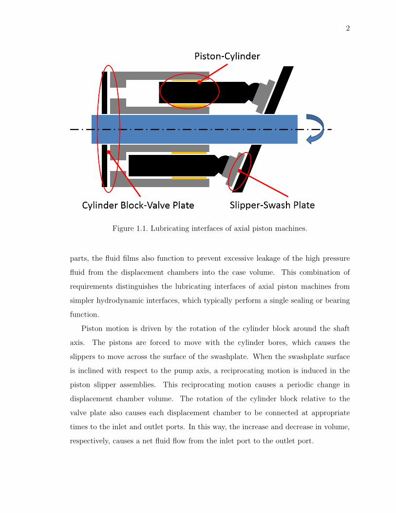
Figure 1.1. Lubricating interfaces of axial piston machines.

parts, the fluid films also function to prevent excessive leakage of the high pressure

fluid from the displacement chambers into the case volume. This combination of

requirements distinguishes the lubricating interfaces of axial piston machines from

simpler hydrodynamic interfaces, which typically perform a single sealing or bearing

function.

Piston motion is driven by the rotation of the cylinder block around the shaft

axis. The pistons are forced to move with the cylinder bores, which causes the

slippers to move across the surface of the swashplate. When the swashplate surface

is inclined with respect to the pump axis, a reciprocating motion is induced in the

piston slipper assemblies. This reciprocating motion causes a periodic change in

displacement chamber volume. The rotation of the cylinder block relative to the

valve plate also causes each displacement chamber to be connected at appropriate

times to the inlet and outlet ports. In this way, the increase and decrease in volume,

respectively, causes a net fluid flow from the inlet port to the outlet port.

3

2. STATE OF THE ART

2.1 Modeling of the Piston Cylinder Interface

Many researchers have worked to understand the operation of the piston cylinder

interface through numerical modeling. Yamaguchi [1] used the Reynolds equation

to perform a stability analysis on pistons of varying shape. The model included the

expansion of the cylinder bore due to high pressure in the displacement chamber, but

did not consider piston micro-motion within the lubricating gap. Analysis presented

in the paper indicate that an axially tapered piston displays improved stability com-

pared to cylindrical designs. Yamaguchi [2] included force equilibrium of the piston

in a later work and concluded that metal to metal contact was almost invariably

present. Sadashivappa et al. [3] developed a simple mathematical model of the piston

cylinder interface to investigate out-of-round and tapered pistons. A comparison to

experiment showed the model under predicted the measured leakage. Gels and Mur-

renhoff [4] developed a FEM based model considering an isothermal, isoviscous piston

cylinder interface. Piston deformation was approximated using beam bending. The

model was used to optimize the lubricating gap length and clearance as well as in-

vestigate tapered shapes for the piston and bushing. Kumar and Bergada [5] showed

piston grooves to be beneficial for small diameter pistons using a rigid body CFD

based model. Agarwal et al. [6] presented a model of the piston cylinder interface in

radial piston pumps considering the Fluid Structure Interaction (FSI) between the

lubricating film and its bounding surfaces. Kuzmin et al. [7] introduced a rigid body

model investigating the relative rotation between piston and cylinder at low speed

conditions.

4

Surface contact and mixed friction are incorporated in some models for conditions

where the imposed load cannot be carried with a full lubricant film. Fang and Shi-

rakashi [8] investigated the incidence of mixed friction between the piston and cylinder

at low operating speeds. The model accounted for axial and rotational motion of the

piston, and assumed a perfectly smooth, cylindrical, rigid piston and cylinder. An

iteration scheme was used to find a piston position in which the external and fluid

pressures balance. In the event of contact between the piston and cylinder a contact

force was implemented to balance the remaining external load. Fatemi et al. [9] pre-

sented a model considering a simplified pressure deformation for the piston cylinder

interface. The model used a modified form of the Reynolds equation to account for

the surface roughness of the piston and cylinder.

Development of the model which forms the basis of the current work began with

Berge [10] (now Ivantysynova) who developed a numerical model to calculate load

support at the piston cylinder interface of axial piston machines. The model consid-

ered a rigid piston and cylinder and both axial and circumferential motion as well as

a non-isothermal temperature field in the lubricating gap. Though load support was

calculated and compared with external loads, the model did not adjust piston motion

to achieve force balance. Wieczorek [11] built on this foundation a model for all three

lubricating interfaces of axial piston machines. His model balanced external forces

with fluid pressure buildup by calculating a piston micro squeeze motion within the

cylinder bore. Ivantysynova and Huang [12] added Elastohydrodynamic deformation

to the model using an influence matrix approach and an external commercial FEM

program. Pelosi and Ivantysynova [13] implemented a thermal model which calculates

the temperature distribution within the piston and cylinder block based on the heat

flux from the lubricating gap. Using this model, Pelosi and Ivantysynova [14] showed

that thermal deformations are critical to the operation of axial piston machines at

high pressures. Pelosi [15] considered as well the effects of thermal stresses on the

deformation of the piston and cylinder block.

5

The model used in this research is adapted from the work of Pelosi [15]. The

primary considerations and shortcomings of Pelosi’s model are discussed below. Later

chapters will describe additions and other improvements which have been made to

the model which is used in the present work.

2.1.1 Piston Dynamics

Figure 2.1 shows the forces acting on the piston during machine operation. The

largest source of external load comes from pressure in the displacement chamber,

pDC . The pressure in each displacement chamber changes with time as the machine

operates as shown in Figure 2.2, as each chamber is connected alternately to the

inlet and outlet ports. This pressure acting on the face of the piston causes an axial

force FDK . This axial force, along with the inertial force due to piston acceleration

FaK and viscous friction from the lubricating gap FTK must be reacted by a normal

force between the slipper and swashplate which is transferred to the piston as FSK .

Because the swashplate may be inclined, FSK may not act along the axis of the piston,

resulting in a side-loading component FSKy. The lubricating interface between piston

and cylinder must carry the radial load on the piston resulting from the sum of

FSKy, the centrifugal acceleration force of the piston FωK , and the viscous drag force

generated by the fluid film between the slipper and swashplate FTG.

Figure 2.1. Forces acting on the piston cylinder interface.

6

Figure 2.2. Measured displacement chamber pressure from Tribo test rig, 500rpm.

7

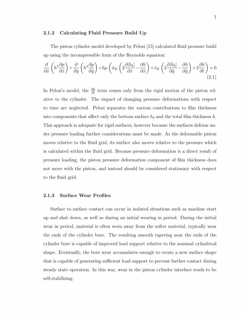
2.1.2 Calculating Fluid Pressure Build Up

The piston cylinder model developed by Pelosi [15] calculated fluid pressure build

up using the incompressible form of the Reynolds equation:

∂

∂x

(h3∂p

∂x

)+∂

∂y

(h3∂p

∂y

)+6µ

(uK

(2∂|hb|∂x− ∂h∂x

)+ vK

(2∂|hb|∂y− ∂h∂y

)+2

∂h

∂t

)= 0

(2.1)

In Pelosi’s model, the ∂h∂t

term comes only from the rigid motion of the piston rel-

ative to the cylinder. The impact of changing pressure deformations with respect

to time are neglected. Pelosi separates the various contributions to film thickness

into components that affect only the bottom surface hb and the total film thickness h.

This approach is adequate for rigid surfaces, however because the surfaces deform un-

der pressure loading further considerations must be made. As the deformable piston

moves relative to the fluid grid, its surface also moves relative to the pressure which

is calculated within the fluid grid. Because pressure deformation is a direct result of

pressure loading, the piston pressure deformation component of film thickness does

not move with the piston, and instead should be considered stationary with respect

to the fluid grid.

2.1.3 Surface Wear Profiles

Surface to surface contact can occur in isolated situations such as machine start

up and shut down, as well as during an initial wearing in period. During the initial

wear in period, material is often worn away from the softer material, typically near

the ends of the cylinder bore. The resulting smooth tapering near the ends of the

cylinder bore is capable of improved load support relative to the nominal cylindrical

shape. Eventually, the bore wear accumulates enough to create a new surface shape

that is capable of generating sufficient load support to prevent further contact during

steady state operation. In this way, wear in the piston cylinder interface tends to be

self-stabilizing.

8

In practice, the piston and cylinder surfaces deviate from their nominal cylindrical

shape by up to tens of microns. This deviation in surface shape is due to both the wear

discussed previously and manufacturing variability. The magnitude of these surface

deviations can easily be larger than the thickness of the fluid film in critical areas

of the lubricating gap and therefore must be considered in the model. In the model

developed by Pelosi [15] only axisymmetric surface profiles are considered. This is

typically adequate only for the piston profile, but the cylinder bore profile is normally

more complex with the wear profile changing in shape and depth at various points

around the circumference of the cylinder bore.

2.1.4 Force Balance

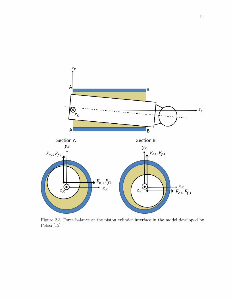
In Pelosi’s model, the force balance calculation includes only fluid forces Ff and

external forces Fe as shown in Figure 2.3. In cases where the fluid forces are not

adequately capable of balancing the external forces, a method of preventing fluid

film collapse is needed. Pelosi implemented a method referred to here as velocity

correction to prevent collapse of the fluid film.

In the velocity correction method correction forces are only calculated after the

force balance loop has converged. This arrangement presents minimal computational

expense but has significant drawbacks. A correction stress σ is first calculated for

each fluid cell whose height is less than the specified minimum. The correction stress

is linearly proportional to the difference between its film thickness and the minimum

specified film thickness as shown in Figure 2.4. Because the surfaces being simulated

are not ideal, the minimum film thickness is defined according to the surface micro-

roughness of the piston and cylinder.

σ (i) =

C (hmin − h (i)) h (i) ≤ hmin

0 otherwise

(2.2)

9

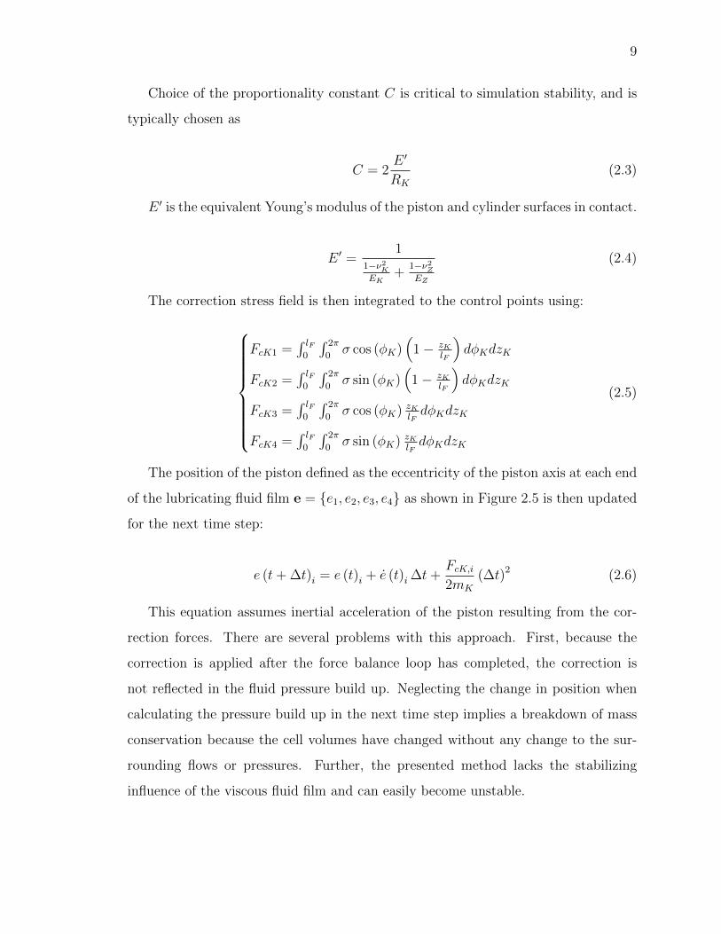
Choice of the proportionality constant C is critical to simulation stability, and is

typically chosen as

C = 2E ′

RK

(2.3)

E ′ is the equivalent Young’s modulus of the piston and cylinder surfaces in contact.

E ′ =1

1−ν2KEK

+1−ν2ZEZ

(2.4)

The correction stress field is then integrated to the control points using:

FcK1 =∫ lF0

∫ 2π

0σ cos (φK)

(1− zK

lF

)dφKdzK

FcK2 =∫ lF0

∫ 2π

0σ sin (φK)

(1− zK

lF

)dφKdzK

FcK3 =∫ lF0

∫ 2π

0σ cos (φK) zK

lFdφKdzK

FcK4 =∫ lF0

∫ 2π

0σ sin (φK) zK

lFdφKdzK

(2.5)

The position of the piston defined as the eccentricity of the piston axis at each end

of the lubricating fluid film e = {e1, e2, e3, e4} as shown in Figure 2.5 is then updated

for the next time step:

e (t+ ∆t)i = e (t)i + e (t)i ∆t+FcK,i2mK

(∆t)2 (2.6)

This equation assumes inertial acceleration of the piston resulting from the cor-

rection forces. There are several problems with this approach. First, because the

correction is applied after the force balance loop has completed, the correction is

not reflected in the fluid pressure build up. Neglecting the change in position when

calculating the pressure build up in the next time step implies a breakdown of mass

conservation because the cell volumes have changed without any change to the sur-

rounding flows or pressures. Further, the presented method lacks the stabilizing

influence of the viscous fluid film and can easily become unstable.

10

One approach to remedying the lack of stability is to limit the areas in which

contact forces can be applied. In practice it is generally acceptable to limit the

calculation of contact forces to the outermost several millimeters of cells on either

end of the lubricating gap. This approach is applicable only to cases of cylindrical

geometry. As the cylinder surface wears, or if a non-cylindrical piston design is

simulated, fluid film breakdown tends to occur further away from the ends of the

fluid film. Because the correction region is limited to small areas near the ends of

the lubricating gap, large areas of collapsed film can occur before any correction force

is calculated. This is demonstrated in Figure 2.6 where there can be a considerable

area of penetration before correction stresses are calculated if only areas to the right

of the green line are considered.

11

Figure 2.3. Force balance at the piston cylinder interface in the model developed byPelosi [15].

12

Figure 2.4. Calculation of correction stress for velocity correction method.

13

Figure 2.5. Piston position in the model developed by Pelosi [15].

14

Figure 2.6. Area of collapsed film occurring with no correction forces calculated whenwear profiles are introduced. Correction stress only considered to the right of greenline.

15

2.2 Experimental Investigation of the Piston Cylinder Interface

The numerical modeling work above is complemented and verified by experimental

work exploring various aspects of piston cylinder operation. Dowd and Barwell [16]

designed a highly simplified test rig to investigate the impact of different material pairs

on the tribological performance of the piston cylinder interface. They were able to

detect contact between the piston and cylinder by monitoring the electrical resistance

between the parts. The test rig was also able to measure friction forces acting on the

cylinder. Construction details of their test rig prevented accurate loading conditions

from being applied to the piston however. Hooke and Kakoullis [17] investigated

the influence of slipper ball socket friction on piston rotation relative to the cylinder

bore by observing piston rotation. The numerical model developed by Fang and

Shirakashi [8] was tested using a specially modified pump. Contact between the piston

and cylinder was again measured by monitoring the electrical resistance between the

parts. Experiment showed that their model over predicted the amount of contact

compared to the experimental data. Manring [18] used a simplified piston cylinder

interface to measure axial friction forces and compared the results to the Stribeck

friction curve. Tanaka et al. [19] investigated run-in wear of various piston profiles

and stiffness values using a simplified two piston pump capable of measuring friction

forces and metal to metal contact. Treuhaft et al. [20] also studied pump run-in wear

behavior using radioactive tracer technology.

A special purpose test rig known as the Tribo was designed and constructed by

Lasaar and Ivantysynova [21] which is capable of measuring the friction forces be-

tween the piston and cylinder. The cross section of the Tribo test pump is shown in

Figure 2.7. A specially designed replaceable bushing is separated from the rotating

cylinder block by a series of hydrostatic bearings. The bushing is held in place only

through a mechanical connection to a force sensor. Any net friction force acting on

the bushing will therefore be measured by the force sensor. Comparing the measured

friction forces to those calculated by the piston cylinder model allows verification of

16

the modeling approach. A pressure sensor is also installed in the same displacement

chamber for the purpose of measuring instantaneous displacement chamber pressure.

Signals from the friction force sensor as well as the pressure sensor are first am-

plified, and then transmitted through a frequency modulated radio telemetry system.

The radio signals are received by an antenna near the pump, and the signal is de-

modulated and recorded using a Data Acquisition (DAQ) system. Due to the design

of the radio telemetry system, only a single sensor channel can be transmitted at one

time. It is therefore necessary to align separately measured data in post-processing

according to a shaft trigger which trips at a specific shaft position once per revolution.

In the test hydraulic circuit implemented by Lasaar and Ivantysynova [21] the

Tribo pump was connected to two other swash plate type machines on a common

shaft. One unit recirculated flow in a test circuit between the Tribo pump and itself,

while the other operated as a secondary controlled motor which provided power to

make up for the losses in the test rig. Friction force measurements made by the test

rig in this configuration contain a high noise level as shown in Figure 2.8. Sources for

the noise can include mechanical vibrations induced in both the rotating group and

also in the test stand itself by the three hydraulic machines. Additionally, because

the majority of the fluid flowing through the Tribo pump was recirculated, control of

the inlet fluid temperature was difficult to maintain. For these reasons a redesign of

the Tribo test rig is desirable. The redesigned test rig described later in section 4.1

is designed to minimize the number of hydraulic machines located on the test stand,

and also simplify the temperature control of the incoming fluid.

Looking again at Figure 2.8, the match between the axial friction profile simulated

by the model of Pelosi [15] and the measured friction leaves much to be desired.

Although the simulated friction line falls within the range of the measured friction

forces, the shape of the simulated friction is poorly reflected in the measurement

data. In the high pressure stroke between 0 − 180◦ the simulated data is rather

noisy, and matches the measurement poorly. In the low pressure stroke between

180− 360◦ the simulated friction profile is nearly flat, while the measurement shows

17

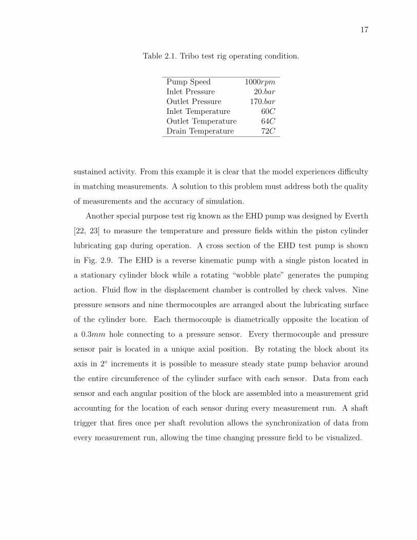
Table 2.1. Tribo test rig operating condition.

Pump Speed 1000rpmInlet Pressure 20.barOutlet Pressure 170.barInlet Temperature 60COutlet Temperature 64CDrain Temperature 72C

sustained activity. From this example it is clear that the model experiences difficulty

in matching measurements. A solution to this problem must address both the quality

of measurements and the accuracy of simulation.

Another special purpose test rig known as the EHD pump was designed by Everth

[22, 23] to measure the temperature and pressure fields within the piston cylinder

lubricating gap during operation. A cross section of the EHD test pump is shown

in Fig. 2.9. The EHD is a reverse kinematic pump with a single piston located in

a stationary cylinder block while a rotating “wobble plate” generates the pumping

action. Fluid flow in the displacement chamber is controlled by check valves. Nine

pressure sensors and nine thermocouples are arranged about the lubricating surface

of the cylinder bore. Each thermocouple is diametrically opposite the location of

a 0.3mm hole connecting to a pressure sensor. Every thermocouple and pressure

sensor pair is located in a unique axial position. By rotating the block about its

axis in 2◦ increments it is possible to measure steady state pump behavior around

the entire circumference of the cylinder surface with each sensor. Data from each

sensor and each angular position of the block are assembled into a measurement grid

accounting for the location of each sensor during every measurement run. A shaft

trigger that fires once per shaft revolution allows the synchronization of data from

every measurement run, allowing the time changing pressure field to be visualized.

18

Figure 2.7. Cross section view of Tribo test rig.

19

Figure 2.8. Sample Tribo test rig measurement compared to a simulation using themodel developed by Pelosi [15].

Figure 2.9. Cross section view of EHD test rig.

20

2.3 Modeling of Tribological Point and Line Contacts

The study of tribological line and point contacts operating in the regime of elas-

tohydrodynamic lubrication (EHL) faces many of the same challenges seen in the

lubricating gaps of axial piston machines. Therefore a review of EHL models and

techniques provides guidance in improving the piston cylinder interface model. Dow-

son and Higginson [24] solved the problem of EHL line contact numerically utilizing

a linear half-space deformation model. An empirical model for fluid density and

viscosity as functions of pressure and temperature was developed by Roelands [25].

Cheng [26] modeled EHL using a two dimensional solution for elliptical contacts, and

compared the developed model to measurement data. Taylor and O’Callaghan [27]

applied a FEM approach to the EHL problem. Brandt [28, 29] presented an adaptive

multi-level approach to solving boundary value problems in which the grid is refined

concurrently with the numerical solution of the problem. Hamrock and Dowson [30]

presented a linear half space model for the calculation of elastic surface deformation

under Hertzian contact stresses. Brewe et al. [31] utilized a grid with variable spac-

ing in the investigation of EHL in point contacts, with additional grid refinement

in the area of maximum pressure. Houpert and Hamrock [32] presented a solution

to the compressible EHL problem using an analytical solution to surface deforma-

tions. Lubrecht et al. [33] applied the multigrid method to the elastohydrodynamic

line contact problem. Kim and Sadeghi [34, 35] investigated the three dimensional

thermal problem in a rolling and sliding point contact. Hu and Zhu [36] presented

a solution for numerically calculating the load support in areas of mixed lubrication

in point contacts by modifying the Reynolds equation in areas of asperity contact.

Goodyer [37] explored transient effects in elastohydrodynamic lubrication. Habchi

[38] achieved perfect agreement between EHL models with loose coupling between

fluid and solid domains and a fully coupled model. For highly loaded contacts, the

loosely coupled models were shown to be more computationally efficient. Each of

21

these resources inspires a closer look at load support in critical areas of the piston

cylinder interface using the novel high definition model described in chapter 5.

2.4 Research Goals

It is believed that during steady state operation there is negligible contact between

the piston and cylinder bore. The goal of this thesis is to achieve a piston cylinder

model which accurately reflects experimentally observed behaviors while demonstrat-

ing full film lubrication. To achieve this the following shortcomings of the existing

model must be addressed:

• Axisymmetric surface profiles are insufficient to realistically describe the shapes

of cylinder bores after pump run-in.

• Pressure buildup calculations within the fluid film neglect key physical effects

relating to squeeze motion of the gap surfaces.

• Handling of conditions of insufficient fluid load support is nonphysical and po-

tentially unstable.

• Grids used for calculation of pressure buildup and surface deformations are too

coarse to capture fine details of fluid film behavior.

It is believed that these shortcomings can be addressed by the following actions:

• Implement realistic surface profiles for all simulations.

• Improve pressure field calculations by including additional physical effects to

the Reynolds equation.

• Improve handling of situations requiring additional load support.

• Implement an adaptive multigrid approach to refine critical areas of the fluid

grid.

22

• Implement a linear half-space deformation model to calculate deformations with

higher resolution than allowed by FEM grid.

The following key points are to be addressed with the Tribo test rig:

• Simplify the hydraulic test circuit to eliminate unnecessary mechanical vibra-

tions.

• Improve control over the inlet oil temperature.

23

3. THE NOVEL PISTON CYLINDER INTERFACE MODEL

This chapter describes the development of a novel piston cylinder model which ad-

dresses the shortcomings detailed in the previous chapter. Model advances which

address the shortcomings detailed previously are:

• Physical effects added to the Reynolds Equation:

– Elastohydrodynamic (EHD) squeeze is added.

– Accurate surface velocities are considered with respect to translational

squeeze.

– Compressible flow is considered.

• Realistic measured surface profiles in one or two dimensions are implemented

for all simulated operating conditions.

• New methods for preventing fluid film collapse are introduced.

• All calculated forces acting on the piston are considered in the force balance.

• Simulation speed and efficiency improved by implementing Finite Element

Method for the thermal analysis.

Figure 3.1 gives an overview of the modeling approach for the piston cylinder

model. A finite volume method is used to calculate pressure build up in the lubricating

gap. This pressure is applied to the surfaces of the solid parts, which results in

deformations of the solid parts calculated using the Finite Elements Method (FEM).

The resulting surface deformations are fed back into the fluid model as updated film

thickness boundary conditions. Viscous dissipation in the lubricating film results

24

Figure 3.1. Piston cylinder modeling approach.

in heat generation which is conducted into the solid parts. This heat conduction

is calculated using a FEM thermal analysis of each part. The calculated surface

temperature distribution is also used to update the boundary conditions for the fluid

model. The calculated temperature distribution within the solid parts is further used

in a FEM analysis accounting for the impact of thermal stresses on the deformation

of the solid parts. The resulting deformations are also fed back to the fluid model

as updated film thickness boundary conditions. The following sections expand on

modeling advances in each section of the model.

3.1 Pressure Field Model and Calculation

To achieve steady state operation, the radial load acting on the piston must be

supported in the lubricating interface entirely through hydrodynamic and hydrostatic

25

pressure buildup. Unlike the other lubricating interfaces, the majority of the piston

cylinder load must be carried by hydrodynamic pressure build up in the fluid film.

Due to the cylindrical shape of the piston cylinder interface any hydrostatic pressure

is distributed approximately equally around the circumference of the piston, providing

little net load support. In some circumstances an imbalance of hydrostatic pressure

can increase the load that must be carried by hydrodynamic build up. The Reynolds

equation used in the present model is adapted from the general form found in Hamrock

et al. [39]:

(3.1)

∂

∂x

(ρh3

12µ

∂p

∂x

)+

∂

∂y

(ρh3

12µ

∂p

∂y

)=

∂

∂x

(ρh (ua + ub)

2

)+

∂

∂y

(ρh (va + vb)

2

)+ ρ (wa − wb)− ρua

∂h

∂x− ρva

∂h

∂y+ h

∂ρ

∂t

To adapt this general equation to the situation of the piston cylinder, two modi-

fications are made. First, the substitution wa − wb = ∂h∂t

is made which includes the

change of film thickness due to both rigid motion and transient pressure deformation.

Second, it is noted that ub = vb = 0 because the cylinder surface is stationary in the

(x, y, z) coordinate system.

The term hK captures those components of the fluid film thickness that move

along with the piston, contributing to the pressure build up in an effect known as

translational squeeze. Specifically, these components are the rigid film thickness, the

thermal deformation of the piston surface, and the wear profile of the piston surface.

Note that pressure deformation of the piston does not contribute to the translational

squeeze effect. This is because the fluid grid is fixed to the bushing. As such, the

calculated pressure and by extension the pressure deformation of the piston are also

non-moving with respect to the bushing. Should the pressure distribution within the

fluid grid change over time, a corresponding change in piston pressure deformation

will be seen. The impact of this effect on pressure build up is properly considered

within the ∂h∂t

squeeze term. The final form of the Reynolds equation used is shown

below.

26

(3.2)

∂

∂x

(ρh3

12µ

∂p

∂x

)+

∂

∂y

(ρh3

12µ

∂p

∂y

)= uK

∂ (ρh)

2∂x+ vK

∂ (ρh)

2∂y+ ρ

∂h

∂t

− ρuK∂hK∂x− ρvK

∂hK∂y

+ h∂ρ

∂t

In some areas the fluid film thickness may drop below a specified minimum allow-

able height. In such cases, pressure build-up is calculated assuming the gap surfaces

are parallel and separated by the minimum allowable height. To implement this

assumption, the Reynolds equation is simplified by substituting zero for any film

thickness gradient terms. The resulting simplified Reynolds equation is then:

(3.3)∂

∂x

(ρh3

12µ

∂p

∂x

)+

∂

∂y

(ρh3

12µ

∂p

∂y

)= uKh

∂ρ

2∂x+ vKh

∂ρ

2∂y+ h

∂ρ

∂t

3.2 Surface Wear Profiles

As described in section 2.1.3, wear profiles are critical to the proper understanding

of the lubricating interfaces. There must therefore be a robust method of simulating

various surface shapes arising from surface wear, manufacturing processes, and various

combinations of these effects. These profiles may be axisymmetric as is usually the

case with pistons or non-axisymmetric which is typical of bushing surfaces.

Because the lubricating fluid film is very thin relative to the diameter of the pis-

ton, the curvature of the interface can be safely neglected. The fluid film can then be

unwrapped as shown in Figure 3.2 where the rectilinear (x, y, z) coordinate system

is introduced. Using this coordinate system, a surface profile is constructed which

defines the deviation from nominal for every (x, y) point for both the piston and cylin-

der. Because the piston translates axially and rotates about its axis during machine

operation, these motions must be accounted for when interpolating the surface shapes

to the fluid geometry.

The surface profile is specified over a user defined grid point by point, so the

model developed in the current work can simulate any measured or theoretical surface

shaping. In the case of a measured profile, a surface profilometer is used to trace the

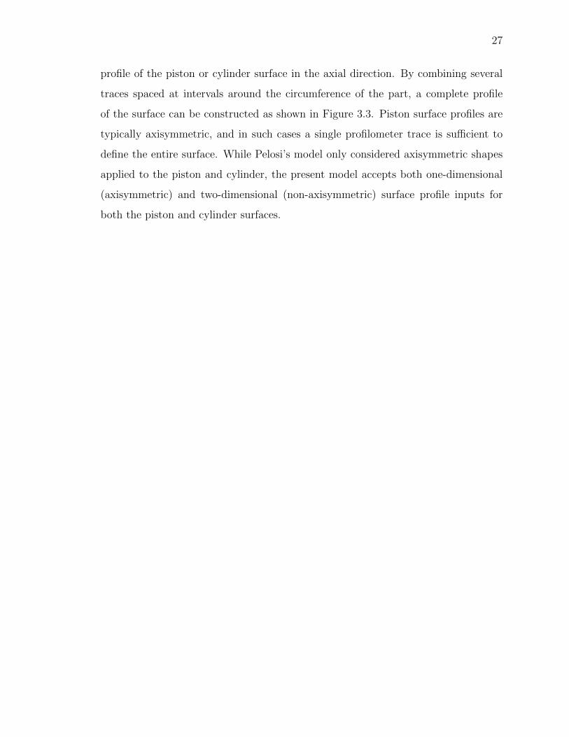
27

profile of the piston or cylinder surface in the axial direction. By combining several

traces spaced at intervals around the circumference of the part, a complete profile

of the surface can be constructed as shown in Figure 3.3. Piston surface profiles are

typically axisymmetric, and in such cases a single profilometer trace is sufficient to

define the entire surface. While Pelosi’s model only considered axisymmetric shapes

applied to the piston and cylinder, the present model accepts both one-dimensional

(axisymmetric) and two-dimensional (non-axisymmetric) surface profile inputs for

both the piston and cylinder surfaces.

28

Figure 3.2. The unwrapped fluid grid.

29

Figure 3.3. Experimental surface profile measurement of a bushing from the Tribotest rig.

30

3.2.1 The Fluid Grid

Figure 3.4 compares the rectangular, structured grid used for the fluid properties

calculations with the triangular, unstructured grid that forms the surface of the solid

bodies of the piston and cylinder. Both of these mesh types are chosen for convenience

and in accordance with the different challenges facing each domain. The solid mesh

must conform to complex and irregular geometry that is present in the piston and

cylinder block solid volumes. For this purpose an unstructured tetrahedral mesh is

well suited. An additional benefit is that such a mesh can be quickly generated by

software using CAD files as input. The generation of solid meshes is accomplished

using an external commercial software. Therein lies the largest disadvantage of the

unstructured tetrahedral mesh. If more detail is desired in a specific region of the

solid body meshes, the entire mesh must be recreated using the external software.

Although this process is relatively fast, it is vastly slower than the generation or

refinement of a structured grid which can be accomplished within the model during

the course of an analysis.

A structured rectangular grid is used for the fluid domain to take advantage of

these strengths. The fluid domain in the piston cylinder interface can be modeled as

an unwrapped rectangular space as described previously, therefore a rectangular grid

serves as a natural subdivision of the domain. The structured grid also maintains

the cell boundaries parallel to the axes used in the discretization of the Reynolds

equation, significantly simplifying the required calculations. Further, because the grid

is defined and constructed within the piston cylinder model at run time, changing the

dimensions or refinement of the grid is minimally expensive.

The finer the solid and fluid grids become, the greater detail is available in the

model. Because the model calculates a fluid structure interaction (FSI), the resolution

of physical effects is limited to the coarsest grid in use. Additional computational re-

sources are consumed by every grid cell, so a mismatch in grid sizes between fluid and

solid meshes results in additional computational resource consumption for minimal

31

additional resolution. The best configuration is approximately shown in Figure 3.4

where the grid sizes are comparable.

Typically the most interesting behavior within the fluid film occurs in the areas

of low film thickness. It would be beneficial to refine the grid in these areas to

a finer resolution so that additional behaviors and phenomena could be explored.

These areas are transient however, and occur in different locations in the fluid film

throughout the operation of the machine. It is therefore impossible to predict where

additional refinement is needed at the time when the solid meshes are being generated.

Chapter 5 details the construction of a model incorporating dynamic grid refinement

to further explore these issues.

32

Figure 3.4. Rectangular fluid grid cells (red) overlaid upon triangular solid body meshfaces (blue).

33

3.3 Solid Body Temperature Distribution

It has been noted that the Finite Volume Method (FVM) temperature field model

implemented by Pelosi [15] required a disproportionately long time to reach conver-

gence when compared with the Finite Element Method (FEM) used to calculate

deformations due to thermal stresses. In an effort to reduce overall simulation times

that in some cases can reach up to a week, a faster method was sought. A new FEM

solver has been implemented inspired by the work of Zecchi [40]. Thermal conduction

within the solid part forms the conduction matrix Kcd. Mixed boundary conditions

are used for areas where convection occurs from the solid part into a fluid volume.

For these boundaries, the terms Kcv and Qcv together define the boundary. Finally,

the heat flux occurring from the lubricating gap is applied using the heat flux vector

Qb. The final result saves a significant amount of simulation time while maintaining

accuracy of the simulation results.

(3.4)KTTi = Qcv +Qb

(3.5)KT = Kcd +Kcv

=

∫V

BTCTBdV + h

∫S

NTNdS

(3.6)Qb =

∫S

NT qbnTdS

(3.7)Qcv = hT

∫S

NTT∞dS

3.4 Solid Body Pressure Deformation

Displacement chamber pressure varies as a function of shaft angle, and acts on

a significant area within the cylinder block. In the model developed by Pelosi [15]

all displacement chambers are subjected to a single uniform pressure equal to that

within the reference bore. However, during machine operation each displacement

34

volume experiences pressures that can at times vary significantly from the pressure

in the neighboring displacement volumes. This effect is most pronounced near the

transitions between the high and low pressure ports when one displacement volume is

connected to high pressure and the other volume is connected to the low pressure port.

During these transitions it is important to consider the pressure deformation caused

by each unique pressure field. The pressure within each displacement volume can

then be considered as a lumped parameter. Due to the uniform pressure field acting

on all surfaces surrounding the displacement volume, a single Influence Matrix (IM)

is defined which corresponds with the application of such a pressure. One such IM is

defined for each separate displacement chamber (DC) volume, as shown in Figure 3.5.

An influence matrix is composed of influence vectors. Each vector describes the effect

or influence over the entire FEM grid surface of a reference pressure applied to a given

portion of the FEM grid. Using the principle of linear superposition, the deformation

of the entire surface given an arbitrary pressure field can be calculated.

Also shown in Figure 3.5 is the Gap surface for which a separate IM is generated

for each triangular face. This discretization allows the non-uniform pressure field

from the lubricating gap to be applied. IMs constitute the main memory requirement

during model execution. Therefore judicious use of IMs is necessary to limit memory

requirements to achievable levels. The model developed by Pelosi [15] neglected the

pressure deformation resulting from neighboring cylinder bores. To approximate the

deformation caused by the pressure fields in neighboring cylinder bores (marked Cyl),

the model developed within this thesis research applies a uniform pressure to these

surfaces which is equal to half the associated displacement chamber pressure. Because

this applied pressure is uniform across the surface, a single IM can be used for each

cylinder bore.

Not shown in Figure 3.5 is the pressure loading on the remaining faces which

experience case fluid pressure. Because the case volume experiences a uniform fluid

pressure, a single IM is used to capture the effect of case pressure over these faces.

35

Figure 3.5. Cylinder block mesh showing face definitions for pressure loading.

36

3.5 Preventing Fluid Film Collapse

In some cases the simulated lubricating fluid film is not capable of supporting a

sufficient amount of the external loads. If nothing is done in these cases to supplement

the simulated load support the piston squeeze motion will continue to move the piston

toward the cylinder surface. If this condition is not resolved, the film will collapse

in the area which lacks support. Eventually, the numerical solution of the fluid film

will diverge, causing the simulation to fail. It is therefore beneficial to implement

some method of preventing extensive fluid film collapse so that the simulation may

converge and produce a complete set of results for analysis. Several methods for

preventing film collapse are presented in this section. All methods presented are

founded upon the correction force vector FcK = {FcK1, FcK2, FcK3, FcK4}. Simulation

stability, performance, and accuracy all depend heavily on how FcK is calculated and

how it affects piston motion.

The proposed solution to the problems described above is to consider the correc-

tion forces FcK directly in the force balance loop as depicted in Figure 3.6. In this

way, the action of the correction forces is appropriately accounted for in the motion of

the piston and the fluid pressure build up at all times. With the correction forces now

included in the force balance loop, the calculation of the correction forces becomes

critically important to the stability and accuracy of the simulation results.

Two methods for calculating FcK are presented in the following sections. Both

methods are implemented and tested in the following chapter and their results com-

pared with measurements.

37

Figure 3.6. Force balance at the piston cylinder interface.

38

3.5.1 Linear Method

The first method considered is inspired by the work of Wieczorek [11]. This

method calculates the correction stress σ according to Equation (2.2) and Figure 3.7.

Correction forces FcK are then calculated according to Equation (2.5). Because the

correction stress is simplified to a linear relationship with respect to surface penetra-

tion, a coefficient must be defined to relate the two quantities. Such a coefficient has

no physical basis, and must be chosen to achieve a combination of desirable perfor-

mance and stability. The value given by Equation (2.3) is found to provide satisfactory

results in most situations. A significantly lower value is required for situations with

unusually thin cylinder walls, to account for the resulting increased compliance of the

surface.

An implicit algorithm is used to calculate the shifting motion of the piston. As

the piston shifting velocity is iterated during the force balance loop, its position is

updated resulting in a change in the amount of surface penetration and therefore

correction forces. Because this method relies on surface penetration to calculate cor-

rection forces, the fluid film thickness is inherently unrealistic within and immediately

surrounding the collapsed area.

39

Figure 3.7. Calculation of linear force balance correction stress.

40

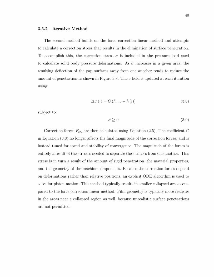
3.5.2 Iterative Method

The second method builds on the force correction linear method and attempts

to calculate a correction stress that results in the elimination of surface penetration.

To accomplish this, the correction stress σ is included in the pressure load used

to calculate solid body pressure deformations. As σ increases in a given area, the

resulting deflection of the gap surfaces away from one another tends to reduce the

amount of penetration as shown in Figure 3.8. The σ field is updated at each iteration

using:

∆σ (i) = C (hmin − h (i)) (3.8)

subject to:

σ ≥ 0 (3.9)

Correction forces FcK are then calculated using Equation (2.5). The coefficient C

in Equation (3.8) no longer affects the final magnitude of the correction forces, and is

instead tuned for speed and stability of convergence. The magnitude of the forces is

entirely a result of the stresses needed to separate the surfaces from one another. This

stress is in turn a result of the amount of rigid penetration, the material properties,

and the geometry of the machine components. Because the correction forces depend

on deformations rather than relative positions, an explicit ODE algorithm is used to

solve for piston motion. This method typically results in smaller collapsed areas com-

pared to the force correction linear method. Film geometry is typically more realistic

in the areas near a collapsed region as well, because unrealistic surface penetrations

are not permitted.

41

Figure 3.8. Calculation of iterative force balance correction stress.

42

4. SIMULATION RESULTS AND MEASUREMENT COMPARISON

The intent of any modeling effort is to predict or to help understand a physical

phenomenon. The piston cylinder model is aimed at both of these goals. For a new

pump or motor design, the model should give a reasonable prediction of performance

and reliability. For an existing design, the model should give insight into the root

cause of problems and predict the effects of design changes. A prerequisite for these

uses is the ability to correctly predict the performance of an existing design. Below,

simulation results are compared with measurements made using a specially built test

rig.

One of the most important outputs of the piston/cylinder model is the energy

dissipated in the lubricating gap. This energy dissipation comes from a combination

of leakage flow and friction forces. A well performing model will predict friction forces

similar in magnitude and shape to experimental values.

4.1 The Tribo Test Rig

To remedy the issues identified with the Tribo test rig in section 2.2 a redesign

of the hydraulic circuit was made. Figure 4.1 shows the updated hydraulic circuit

for the Tribo test rig. The heart of the test rig is the previously described Tribo

pump/motor with its associated sensors and telemetry system. The pump/motor

is now the only hydraulic machine on the test stand and is driven by a three phase

electric induction motor controlled by a regenerative variable frequency drive. A drive

enable circuit fulfills a safety function by disabling the electric motor in the event of

any emergency stop button being pressed or a fault detection by the DAQ system.

43

Figure 4.1. Hydraulic circuit for Tribo test rig.

When the drive is actively controlling the electric motor, voltage is applied to an

enabling valve which allows hydraulic oil from the lab hydraulic supply to reach the

Tribo pump/motor. Fluid pressures at the inlet and outlet of the Tribo pump/motor

are controlled by variable pressure relief valves. In this configuration, oil from the

temperature controlled main power supply passes through the Tribo pump once and

then returns back to the main reservoir for cooling. This arrangement vastly simplifies

the requirement of maintaining the inlet temperature at the desired set point. Fluid

pressures and temperatures are measured at the pump/motor inlet, outlet, and case

drain ports.

44

4.2 Tribo Test Rig Data Processing

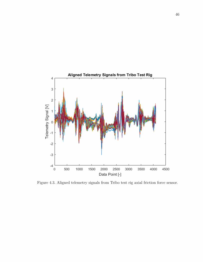
Processing the data from the Tribo test rig presents several challenges. The

telemetry system can only transmit a single channel at a time. Because the three

measurement channels cannot be recorded concurrently, it must be assumed that

measurements are made in steady state operation. This assumption implies that

data captured from every revolution should mirror every other revolution as is the

case for the displacement chamber pressure signal shown in Figure 4.2. In practice

small differences exist in the friction data from each revolution as shown in Figure 4.3.

For this reason, data is collected across many revolutions, and the typical behavior is

compared against simulation.

Once friction measurements for every revolution have been aligned according to

the shaft trigger, a histogram is taken for each angle as shown in Figure 4.4. All of the

individual histograms are then oriented vertically and combined into a time varying

histogram contour plot as shown in Figure 4.5. The color scale of the plot represents

the occurrence frequency of each friction value at a given shaft angle. All occurrence

frequencies are normalized such that they fall on the interval [0, 1]. As a result, shaft

angles with more consistent data will generate higher occurrence frequencies relative

to shaft angles with more measurement noise.

To compare measurements with simulation results, the simulated friction curve is

overlaid upon the contour plot. Because the force sensor used in the Tribo test rig is a

piezoelectric type sensor, it is capable of measuring only dynamic forces. This means

that the recorded data cannot indicate the exact magnitude of the force at a given

instant of time, only the change in force with time. As a result, it is unknowable from

the measured data when the friction curve transitions between positive and negative.

To compensate for this unknown, the measured friction values are shifted vertically to

find a best fit with the simulated curve. This shifting is accomplished automatically

using a MATLAB comparison script.

45

Figure 4.2. Aligned telemetry signals from Tribo test rig displacement chamber pres-sure sensor.

Similarly, because the exact shaft angle which the shaft trigger indicates is un-

known, a shift in the measured shaft angle axis is also permitted. This shift is again

computed automatically using the MATLAB comparison script to ensure fair com-

parison between measurement and various different simulation results.

46

Figure 4.3. Aligned telemetry signals from Tribo test rig axial friction force sensor.

47

Figure 4.4. Creation of a histogram from a single shaft angle of multiple revolutions.

Figure 4.5. Creation of a time-varying histogram contour from individual histograms.

48

4.3 Measured Operating Conditions

Within each following section is presented a table containing information about

the steady-state operating conditions during the measurement. Following the table

is a figure comparing simulated and measured friction forces for several variations of

the piston cylinder model. The various models are as follows:

• Top Left: Full model, including all physical effects discussed in Chapter 3.

Linear force correction method is used.

• Top Right: Full model, except EHD Squeeze as described in Section 3.1 is

neglected.

• Middle Left: Full model, with incompressible oil.

• Middle Right: Full model, with piston pressure deformation included in hK as

described in Section 3.1.

• Bottom Left: Full model, using iterative force correction method as described

in Section 3.5.2.

• Bottom Right: Full model, using velocity correction method as described in

Section 2.1.4.

4.3.1 500rpm 80bar

This operating condition, defined in Table 4.1, was measured using the Tribo test

rig with a previously unused bushing. Because of the initial condition of the bushing,

and the relatively low power operating condition, it is assumed that minimal wear

occurred prior to the measurement. Therefore, for the simulation of this operating

condition the measured wear profile was scaled down as shown in Figure 4.6.

A comparison of the various models in Figure 4.7 shows that the full model,

along with the model lacking EHD squeeze, and the model considering incompressible

49

Table 4.1. Operating condition information 500rpm 80bar.

Pump Speed 503rpmInlet Pressure 19barOutlet Pressure 80.barInlet Temperature 42COutlet Temperature 43CDrain Temperature 44C

flow give similar results that closely match measurements. When piston pressure

deformation is included in the translational squeeze, the simulated friction force begins

to diverge notably from the measured profile. The iterative force balance method

results in a very low friction force compared to measurement. This is consistently seen

throughout all comparisons, and is due to higher film thicknesses in the critical areas

of the film resulting from the iterative method of force correction. This phenomenon

is shown in Figure 4.8 The velocity correction method performs similarly to the full

model.

50

Figure 4.6. Modified wear profile for the bushing used in the presented measurements.

51

Figure 4.7. Simulated friction vs. measurement. Tribo test rig, 500rpm 80bar 42C.From top left: full code, without transient squeeze, with incompressible Reynolds,without translational squeeze, iterative force correction, velocity correction.

52

Figure 4.8. Simulated film thickness for full code (top) and change in film thicknessdue to iterative force correction (bottom). Tribo test rig, 500rpm 80bar 42C.

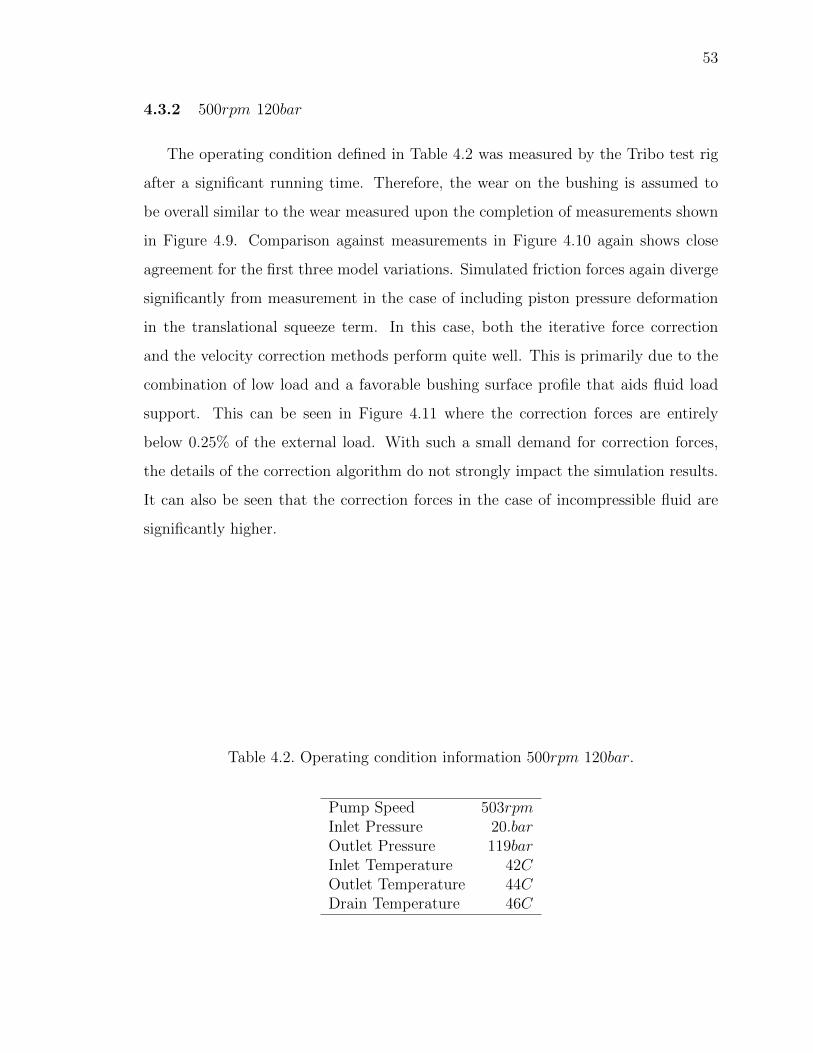
53

4.3.2 500rpm 120bar

The operating condition defined in Table 4.2 was measured by the Tribo test rig

after a significant running time. Therefore, the wear on the bushing is assumed to

be overall similar to the wear measured upon the completion of measurements shown

in Figure 4.9. Comparison against measurements in Figure 4.10 again shows close

agreement for the first three model variations. Simulated friction forces again diverge

significantly from measurement in the case of including piston pressure deformation

in the translational squeeze term. In this case, both the iterative force correction

and the velocity correction methods perform quite well. This is primarily due to the

combination of low load and a favorable bushing surface profile that aids fluid load

support. This can be seen in Figure 4.11 where the correction forces are entirely

below 0.25% of the external load. With such a small demand for correction forces,

the details of the correction algorithm do not strongly impact the simulation results.

It can also be seen that the correction forces in the case of incompressible fluid are

significantly higher.


Pump Speed 503rpmInlet Pressure 20.barOutlet Pressure 119barInlet Temperature 42COutlet Temperature 44CDrain Temperature 46C

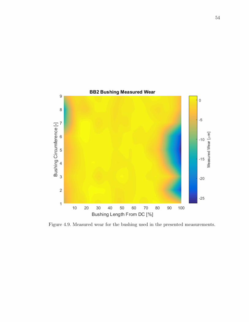
54

Figure 4.9. Measured wear for the bushing used in the presented measurements.

55


56

Figure 4.11. Correction forces normalized to external forces for full model (top) andmodel with incompressible fluid (bottom).

57

4.3.3 500rpm 150bar

As in the previous operating condition, the operating condition defined in Table 4.3

is assumed to have a fully developed wear profile on the bushing surface. Comparing

measurements to simulation results in Figure 4.12 shows that all models reflect quite

closely the measured friction. It can be noted that neglecting either EHD squeeze or

compressible flow leads to numerical instabilities in the predicted friction. All other

model variations for this operating condition show negligible differences relative to

one another.


Pump Speed 503rpmInlet Pressure 21barOutlet Pressure 150.barInlet Temperature 41COutlet Temperature 44CDrain Temperature 47C

58


59

4.3.4 500rpm 190bar

As previously, the operating condition defined in Table 4.4 considers a fully de-

veloped wear profile on the bushing surface. Comparing measurements to simulation

results in Figure 4.13 shows that all models again reflect quite closely the measured

friction. It is again the case that neglecting either EHD squeeze or compressible flow

leads to numerical instabilities in the predicted friction. All other model variations

for this operating condition show negligible differences relative to one another.


Pump Speed 502rpmInlet Pressure 23barOutlet Pressure 194barInlet Temperature 42COutlet Temperature 46CDrain Temperature 50.C

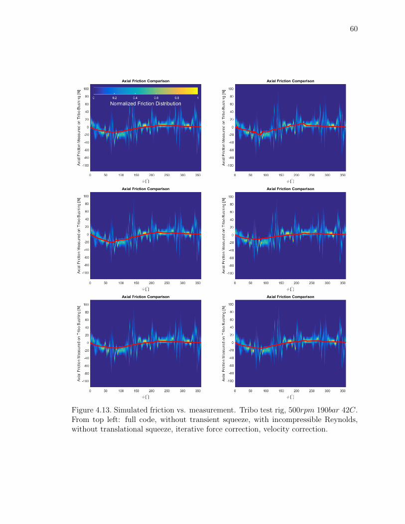
60


61

4.4 Evaluating the Models

The impact of each modification to the model can be identified from the results

presented in the previous section. The iterative force correction method does not

consistently match measured friction values. Although the friction predictions made

by the velocity correction code are satisfactory in the examples presented, the method

violates the conservation of mass and introduces numerical instabilities as discussed

previously. The models neglecting EHD squeeze produces increased numerical insta-

bilities during the high pressure stroke. This problem is exacerbated at higher speeds.

Incorrectly including piston pressure deformation in the translational squeeze term

results in predicted friction forces which do not match measurements as reliably as

the full model. Modeling the fluid as incompressible begins to produce numerical

instabilities as the operating pressures rise, though the overall predicted friction force

agrees well with measurement. Additionally, the incompressible fluid leads to dra-

matically increased correction forces. For these reasons, the full model is chosen for

continued development.

In all the examples presented the full model is able to satisfactorily match the

measured axial friction values while requiring relatively small correction forces. How-

ever the full model continues to predict areas of collapsed fluid film where full film

lubrication is assumed.

62

5. THE HIGH DEFINITION LUBRICATION MODEL

As discussed in Section 3.5, much work has been done to solve an array of problems

centered around collapsed regions of the lubricating film. It has been noted that

swash plate type axial piston machines that operate successfully in practice continue

to show collapsed film regions when simulated. Efforts by Pelosi [15] to include

thermal and pressure deformations, along with the addition of the effects described

in chapter 3 have improved simulation accuracy, but have not resulted in elimination

of such collapsed regions. The most likely causes of the continuing occurrence of these

collapsed regions are:

• Excessive coarseness of the fluid grid.

• Excessive coarseness of the FEM solid body deformation analysis.

Typical fluid grid and FEM element edge dimensions used for this work are ap-

proximately 3% of the piston diameter. This scale is chosen to:

• Reduce simulation time requirements. A typical simulation takes from two to

five days to complete.

• Reduce simulation memory requirements. A typical piston cylinder simulation

requires approximately 2GB of memory.

As grid spacing becomes finer, simulation times increase and fewer simulations

can be run concurrently due to hardware memory limitations. To maintain adequate

computational throughput, a sacrifice in model fidelity must be made in favor of

computational time and resource conservation. This chapter details the construction

63

of a High Definition (HD) model to investigate the assumption that finer scales in

both fluid and solid domains will improve calculated load support. Key improvements

implemented in this model are:

• Adaptive multigrid applied to pressure calculations.

• Linear half-space deformation model to calculate surface deformations in high

definition.

• A fluid properties model extended to high pressures.

5.1 Modeling Approach

Although the best strategy in terms of fidelity, refining the fluid and solid domain

meshes in the piston cylinder analysis is prohibitively expensive in terms of computa-

tional time. The analysis of each time step must complete before the model can move

on to the next time step. This constrains the piston-cylinder simulation to a minimal

amount of parallelization, and a long simulation time. To take advantage of available

parallel computing resources, a non-sequential approach must be adopted. Accord-

ingly, the HD model is intended to revisit the areas of collapsed film from an analysis

of the standard piston cylinder model. Boundary and loading conditions taken from a

single collapsed region form the basis for each HD analysis. Within each HD analysis

both the fluid grid and the pressure deformation calculations are dynamically refined

to a much finer grid where additional detail is required. The result is a much greater

insight into the behavior and load carrying ability of the fluid film in these areas that

collapse in the standard analysis.

5.1.1 Generation of Inputs

MATLAB scripts are used to analyze the outputs of the piston cylinder model.

These scripts search through every time step of the simulation results to find every

area of collapsed film.

64

5.1.1.1 Analysis Region

First, an analysis region must be defined. In this case, regions where contact stress

is calculated by the standard model are clearly of interest. It is desirable however

to have a slightly larger domain over which the model can solve for the pressure

distribution. Therefore all surrounding areas with film thickness less than a critical

value of 3hmin are also included for analysis.

It is likely that multiple areas of contact stress will be computed by the standard

definition piston cylinder model during a single time step. In this circumstance a

means of considering the individual areas in separate analyses is desirable. These

goals can be accomplished by the following method. The results can be seen in

Figure 5.1 and Figure 5.2.

1. Construct a matrix with each entry representing a cell in the rectangular fluid

grid from the piston cylinder model.

2. Scan the entire grid, marking each cell that falls below the predetermined min-

imum film thickness.

3. Scan the marked cells for the first cell that is not assigned to an analysis patch,

and assign a patch number.

• Loop through the newly identified patch, and incorporate all bounding

elements with low film thickness.

• Continue adding bounding elements until the analysis patch no longer

grows.

• Repeat this step until all elements with low film thickness have been as-

signed to an analysis patch.

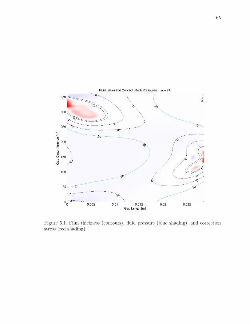
65

Figure 5.1. Film thickness (contours), fluid pressure (blue shading), and correctionstress (red shading).

66

Figure 5.2. Regions of interest defined based on film thickness.

67

5.1.1.2 Boundary Conditions

The following properties are defined for each cell within the analysis patch:

• Location within the gap.

• Total film thickness.

• Translating portion of film thickness.

• Fluid pressure.

• Correction pressure.

• Bounding surface temperature.

• Squeeze motion due to rigid body motion and transient deformation.

• Connectivity to other cells in analysis patch.

The MATLAB script builds an input file for each analysis patch that defines the

above information for each grid point.

Pressure

Pressure boundaries can be set according to the gap pressure field present in the

standard piston cylinder model analysis.

Load

The required load support can be well defined based on standard piston cylinder

model outputs. It consists of the load supported by fluid and contact pressure fields

in the analysis region. These fields can be summed, and the resultant load force

magnitude integrated throughout the area.

Film Thickness

The fluid film thickness and shape are critical in enabling hydrodynamic load

support. As such, a realistic starting estimate of film thickness must be made. This

can also be achieved by interpreting the results of the standard piston cylinder model.

68

The film thickness is taken from the standard piston cylinder model, before it is

saturated to the specified minimum thickness.

If the load support calculated by the HD model is to balance the required load,

there must exist a degree of freedom by which the calculated load support can be

affected. To achieve this degree of freedom, a variable vertical offset is added to the

film thickness. Iterations of the analysis are made, with the initial large offset incre-

mentally decreasing until either the fluid film collapses or the load is fully supported.

In cases where the fluid film ultimately collapses, the highest achieved load support

is recorded.

5.1.2 Surface Pressure Deformation

In addition to the nominal surface shaping given by the boundary conditions, the

surface shape will also depend on the pressure field calculated by the HD model.

A method is needed to calculate the pressure deformation of the bounding surfaces

in widely varying levels of detail. Some areas where the grid is dynamically resized

to a fine spacing require surface deformations to be calculated at a matching level

of detail. Other areas that are not refined can use a similarly coarse calculation

of surface deformation without penalty. The influence method used by Pelosi [15],

although well suited to the standard piston cylinder model, is not suitable for the

HD model because the FEM mesh must be defined prior to the analysis. Because the

level of refinement varies significantly throughout the analysis region, any method

that requires a predefined mesh must provide sufficient resolution everywhere. This

would provide excessive refinement throughout the majority of the grid, leading to

prohibitive computational expense and memory requirements during the analysis.

A linear half-space model developed by Hamrock and Dowson [30] is chosen to

meet these requirements. In this model, the analysis region is broken up into rectan-

gles of constant pressure. The deformation of any point within the region can then

be calculated using the principle of linear superposition. It is important to note here

69

that the surfaces in the analysis region have already been deformed by the pressure

and contact stress fields calculated by the standard piston cylinder model. Therefore

the pressure field used in the half-space calculations should be the difference between

the pressure calculated by the HD model and the pressure and contact stress fields

calculated by the standard piston cylinder model.

Referring to Figure 5.3, deformation of the elastic half space is calculated using:

w =2P

π

∫ a

−a

∫ b

−b

1√(Y − Y1)2 + (X −X1)

2dX1dY1 (5.1)

Here, the dimensionless pressure P is calculated:

P =pfluid,HD + pcontact,HD − pfluid,Standard − pcontact,Standard

E ′(5.2)

E ′ is the equivalent stiffness of the piston and cylinder surfaces as calculated in

Equation (2.4). Figure 5.4 gives an example of the superposition of deformations

resulting from two rectangular areas of pressure applied to the surface.

Pressure deformation calculations begin on the coarsest grid level,shown in red

in Figure 5.5 with a unique pressure applied to the rectangular area of each fluid

cell. As the grid is refined, new cell centroids (shown in blue) are created that fall

midway between existing cell centroids. By introducing smaller cells during the grid

refinement process, the pressure loading of the half space can become more finely

detailed. The deformation resulting from the coarser grids is already applied to the

surface before the finer grid loading is calculated. Therefore it is necessary to only

consider the difference (shown in blue) between the pressure already accounted for

and the newly added pressure (green). By nature of its construction, each new grid

point is placed on the border of two or more cells existing in the coarser grid. So it is

the difference between the finer cell’s calculated pressure and the linearly interpolated

pressure from the coarser grid at the same location that is applied to the finer grid.

This process repeats for each additional grid level.

70

Figure 5.3. Section of linear half space domain showing applied pressure in yellowrectangle centered at point (X1, Y1), and deformation calculated at point (X, Y ).

Figure 5.4. Example of superposition of two rectangular areas of applied pressure onhalf space deformation model.

71

Figure 5.5. Pressures applied to deformation model in refined areas.

72

5.1.3 Adaptive Grid Refinement

A rectangular structured grid is utilized. This allows for significant simplification

of calculations (e.g. a constant spacing between every cell), however a method of

refining parts of the grid must be developed. Mesh refinement is an automated process

within the HD model. This is accomplished using an adaptive multigrid approach

in which the finer mesh levels are only defined within selected portions of the global

mesh. The results from these refined areas are then used to update the coarse mesh

as with a standard geometrical multigrid approach.

The simulation begins with its coarsest grid, as given from the standard piston

cylinder model. The model solves this grid until convergence has been reached. A

specified percentage of the grid with the lowest film thickness is then refined to form

the next finer level. Bilinear interpolation is used to initialize the fluid and surface

parameters for the newly created grid points. The model then solves the multigrid

problem, using the original coarse grid to speed convergence for low frequency effects,

and the higher resolution refined grids to calculate finer details. This refinement

process continues, with the specified percentage of each level forming the grid for

the next level, until the specified number of refinement levels have been created.

When the fully refined system converges, the load support is compared with the

required support to determine whether to repeat the analysis with a lower starting

film thickness or terminate the simulation if sufficient load support is achieved.

5.1.4 Fluid Properties

The oil used in experiments at the Maha Fluid Power Research Center has been

characterized over a range of temperatures from 25C to 120C and pressures from

100kPa to 137.8MPa. Because the HD model may generate pressures well in excess of

these measurements, a more general oil model is required. According to Roelands [25],

the variation of viscosity with respect to pressure and temperature of a lubricating

oil can be described as:

73

log (1000µ) = G0

(1 + p

1.96133·108)Z0(

1 + T135

)Sa− 1.2000 (5.3)

This equation was fitted to the measured data for the oil in use at the Maha Lab.

Fluid density can be modeled as:

ρ = ρ0

(1 +

0.6p

1 + 1.7p

)+ cρT (T − T0) (5.4)

This equation was also fitted to measured data from the oil used in the Maha

Lab. Within the range of measured fluid property data, an empirical fit is used to

more closely approximate the measured data. As the fluid pressure approaches the

boundary of the measured range, the model smoothly transitions to the Roelands

model described. The model developed in this research is capable of calculating fluid

properties up to a pressure of 1GPa.

5.1.5 Pressure Build Up

As with the standard piston cylinder model, pressure build up is computed using

the Reynolds equation. However because the HD model begins with different assump-

tions the derivation is somewhat different. Again, the starting point is the general

form found in Hamrock et al. [39]:

(5.5)

∂

∂x

(ρh3

12µ

∂p

∂x

)+

∂

∂y

(ρh3

12µ

∂p

∂y

)=

∂

∂x

(ρh (ua + ub)

2

)+

∂

∂y

(ρh (va + vb)

2

)+ ρ (wa − wb)− ρua

∂h

∂x− ρva

∂h

∂y+ h

∂ρ

∂t

Because the bottom cylinder surface is considered to be fixed in this analysis, and

surface velocity is constant the equation simplifies to:

(5.6)

∂

∂x

(ρh3

12µ

∂p

∂x

)+

∂

∂y

(ρh3

12µ

∂p

∂y

)= ua

∂

∂x

(ρh

2

)+ va

∂

∂y

(ρh

2

)+ ρwa − ρua

∂h

∂x− ρva

∂h

∂y+ h

∂ρ

∂t

74

Fluid expansion with respect to time is neglected, as it is assumed to provide

only a small contribution to pressure build up in the areas of interest. However,

to capture the motion of the piston surface accurately, the hK term must be used

in the translational squeeze term, as described in section 2.1.2. Also similarly to

the standard piston cylinder model, the squeeze term wa is composed of rigid piston

motion and transient squeeze calculated in the standard model.

(5.7)

∂

∂x

(ρh3

12µ

∂p

∂x

)+

∂

∂y

(ρh3

12µ

∂p

∂y

)= ua

∂

∂x

(ρh

2

)+ va

∂

∂y

(ρh

2

)+ ρ

∂h

∂t− ρua

∂hK∂x− ρva

∂hK∂y

5.1.6 Result Compilation

The results of each patch can be displayed individually as shown in Figure 5.6

which shows fluid film thickness contours along with pressure build-up throughout

the analysis area. In the case shown, the patch is capable of supporting the required

load while maintaining significantly higher fluid film thicknesses compared to the

standard piston cylinder model.

After all the patches have been individually analyzed, the collective results are

compiled by a post-processing MATLAB script. The script loads the outputs from

every analysis and reads both the required and calculated load support. These values

can then be graphically displayed as shown in Figure 5.7. Each circle represents the

analysis of a single patch of collapsed film. Circle size corresponds to the load support

required of each patch. Horizontal position indicates the shaft angle at which each

patch occurred. Vertical position indicates the percentage of required load which is

supported using the HD model.

Figure 5.7 shows that the majority of patches analyzed achieve 100% of the re-

quired load support. However, there remain many patches which are not capable of

supporting any significant load. One possible reason for this is the decoupled na-

ture of the HD code. Load support calculated on the highly refined mesh of the HD

75

Figure 5.6. Sample HD analysis output for single analysis region. Color indicatesfluid pressure in bar, contours indicate film thickness in µm.

model is not communicated to the piston cylinder model’s force balance calculations

or its pressure deformation calculations. Improved results can be expected if the load

support from the refined patches is considered within the piston cylinder model.

76

Figure 5.7. Sample HD analysis cumulative output. Circle size indicates requiredload support. Tribo Test Rig, 500rpm, 120bar.

77

6. INTEGRATING HD PRESSURE CALCULATIONS WITH THE

PISTON CYLINDER MODEL

A first step to remedy the shortcomings of the HD model presented in the previous

chapter is to integrate its adaptive fluid domain calculations directly into the piston

cylinder model presented in Chapter 3. Numerical errors in the solution of Reynolds

equation are likely in the piston cylinder model when the film thickness changes

dramatically in the space of one grid cell. Therefore refining only the piston cylinder

model’s pressure calculations is likely to improve the accuracy of the simulation even

with standard definition surface deformation calculations. An important advance in

this research is the development of a robust physics based force balance solver.

6.1 Pressure Buildup Calculations

A simplified form of the Reynolds equation for the piston cylinder interface intro-

duced by Shang [41] is implemented:

∂

∂x

(ρh3

12µ

∂p

∂x

)+

∂

∂y

(ρh3

12µ

∂p

∂y

)=ut2

∂ (ρh)

∂x+vt2

∂ (ρh)

∂y+ ρ

∂h

∂t total(6.1)

Where all changes in fluid film thickness with respect to time are captured in the

term:

∂htotal∂t

= −hcurrent − hpreviousdt

(6.2)

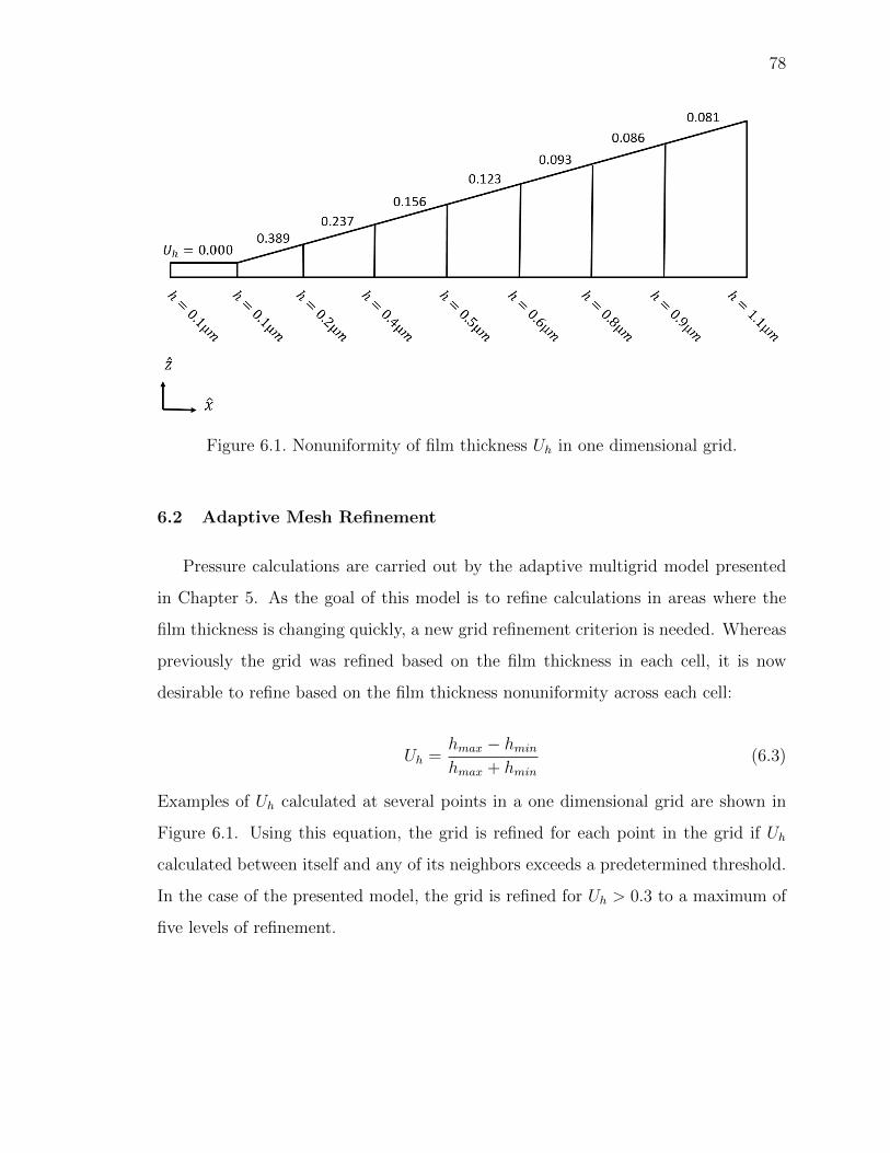
78

Figure 6.1. Nonuniformity of film thickness Uh in one dimensional grid.

6.2 Adaptive Mesh Refinement

Pressure calculations are carried out by the adaptive multigrid model presented

in Chapter 5. As the goal of this model is to refine calculations in areas where the

film thickness is changing quickly, a new grid refinement criterion is needed. Whereas

previously the grid was refined based on the film thickness in each cell, it is now

desirable to refine based on the film thickness nonuniformity across each cell:

Uh =hmax − hminhmax + hmin

(6.3)

Examples of Uh calculated at several points in a one dimensional grid are shown in

Figure 6.1. Using this equation, the grid is refined for each point in the grid if Uh

calculated between itself and any of its neighbors exceeds a predetermined threshold.

In the case of the presented model, the grid is refined for Uh > 0.3 to a maximum of

five levels of refinement.

79

6.3 A New Force Balance Solver

In the work of Pelosi [15] Newton’s root finding method is used to find a shifting

velocity e which balances the forces. Newton’s method assumes the second deriva-

tive of the function is continuous. In this case the function whose roots are to be

found is the force balance of the piston including the correction forces described in

Section 3.5.1. The second derivative of piston force imbalance is discontinuous at the

piston position at which contact forces begin to occur. Therefore Newton’s method is

not guaranteed to achieve a stable solution to the force balance problem and a more

robust method is required.

Because the force balance of the piston is based in physics, knowledge of the

physics involved can be used to formulate a new force balance algorithm. The funda-

mental purpose of the force balance algorithm is to maintain the piston in a state of

force equilibrium by changing its shifting motion e. From Newton’s laws of motion we

know that any object in a state of force imbalance will move in accordance with the

imbalanced forces. Accordingly the following approach is devised. First a unit vector

dv is defined based on the direction of force imbalance dF acting on the piston.

dF = Ff + Fe + FcK (6.4)

dv = − dF

|dF|(6.5)

Then a line search is performed in the direction defined by dv by varying the

change in velocity ∆v until a minimum |dF| is found.

etrial = e + ∆v · dv (6.6)

Once a minimum is found a new search direction is found using Equation (6.4).

This process is iterated until |dF| falls below a predetermined threshold.

80

7. HIGH DEFINITION PISTON CYLINDER SIMULATION

RESULTS AND MEASUREMENT COMPARISON

The EHD test rig introduced in Section 2.2 was used by Pelosi [15] to record the

temperature and pressure distribution in the piston cylinder lubricating gap. The

operating condition is detailed in Table 7.1. These measurements are here compared

to the simulation outputs of the high definition piston cylinder model. Cylinder bore

temperature and lubricating gap pressures are presented as described in Section 3.2.

Table 7.1. EHD test rig operating condition.

Pump Speed 1000rpmInlet Pressure 25barOutlet Pressure 175barInlet Temperature 43COutlet Temperature 45CDrain Temperature 55C

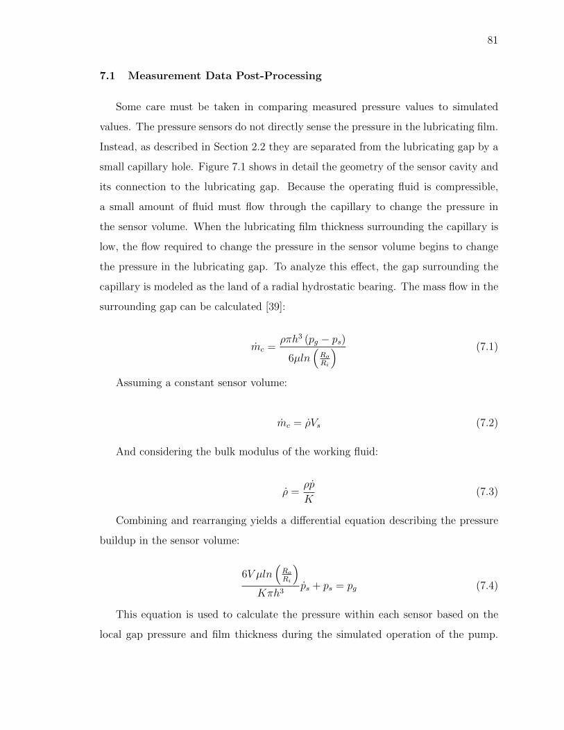
81

7.1 Measurement Data Post-Processing

Some care must be taken in comparing measured pressure values to simulated

values. The pressure sensors do not directly sense the pressure in the lubricating film.

Instead, as described in Section 2.2 they are separated from the lubricating gap by a

small capillary hole. Figure 7.1 shows in detail the geometry of the sensor cavity and

its connection to the lubricating gap. Because the operating fluid is compressible,

a small amount of fluid must flow through the capillary to change the pressure in

the sensor volume. When the lubricating film thickness surrounding the capillary is

low, the flow required to change the pressure in the sensor volume begins to change

the pressure in the lubricating gap. To analyze this effect, the gap surrounding the

capillary is modeled as the land of a radial hydrostatic bearing. The mass flow in the

surrounding gap can be calculated [39]:

mc =ρπh3 (pg − ps)

6µln(Ro

Ri

) (7.1)

Assuming a constant sensor volume:

mc = ρVs (7.2)

And considering the bulk modulus of the working fluid:

ρ =ρp

K(7.3)

Combining and rearranging yields a differential equation describing the pressure

buildup in the sensor volume:

6V µln(Ro

Ri

)Kπh3

ps + ps = pg (7.4)

This equation is used to calculate the pressure within each sensor based on the

local gap pressure and film thickness during the simulated operation of the pump.

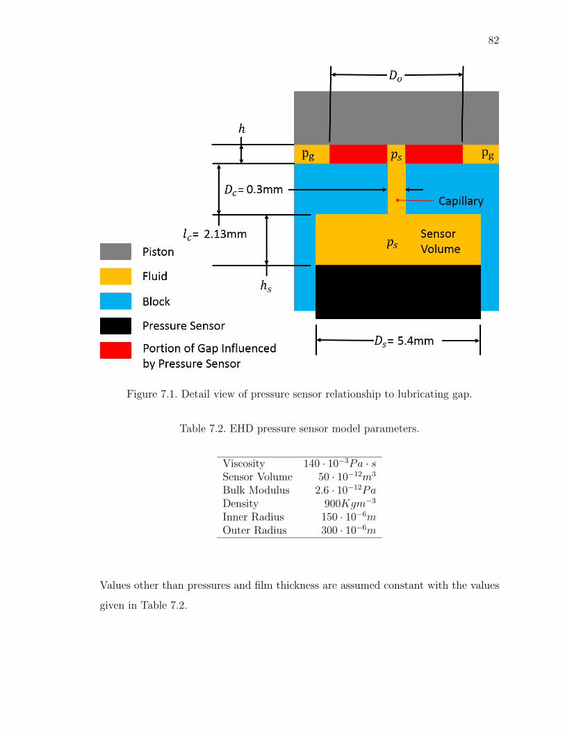
82

Figure 7.1. Detail view of pressure sensor relationship to lubricating gap.

Table 7.2. EHD pressure sensor model parameters.

Viscosity 140 · 10−3Pa · sSensor Volume 50 · 10−12m3

Bulk Modulus 2.6 · 10−12PaDensity 900Kgm−3

Inner Radius 150 · 10−6mOuter Radius 300 · 10−6m

Values other than pressures and film thickness are assumed constant with the values

given in Table 7.2.

83

7.2 Simulation Comparison to Measurement

7.2.1 Cylinder Surface Temperature

Figure 7.2 shows the measured and simulated temperature fields of the cylinder

surface. Good agreement is achieved between the converged simulation and the steady

state measurements both in absolute value and overall pattern.

84

Figure 7.2. Temperature field of EHD cylinder surface measured (top) and simulated(bottom).

85

7.2.2 Film Pressure

Figures 7.3 through 7.6 show simulated sensor pressure data for the HD piston

cylinder model and the standard piston cylinder model compared to measurement.

Good overall agreement is achieved by both models in comparison to the measured

data. However, the HD piston cylinder model generates a pressure profile that more

consistently matches the measurements compared to the standard piston cylinder

model. This is evident primarily in the low pressure area on the left side of the

figures.

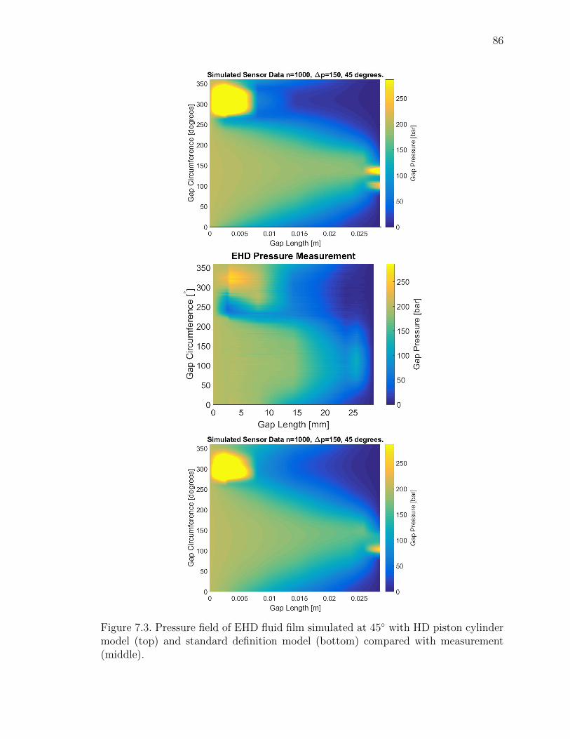
86

Figure 7.3. Pressure field of EHD fluid film simulated at 45◦ with HD piston cylindermodel (top) and standard definition model (bottom) compared with measurement(middle).

87


88


89


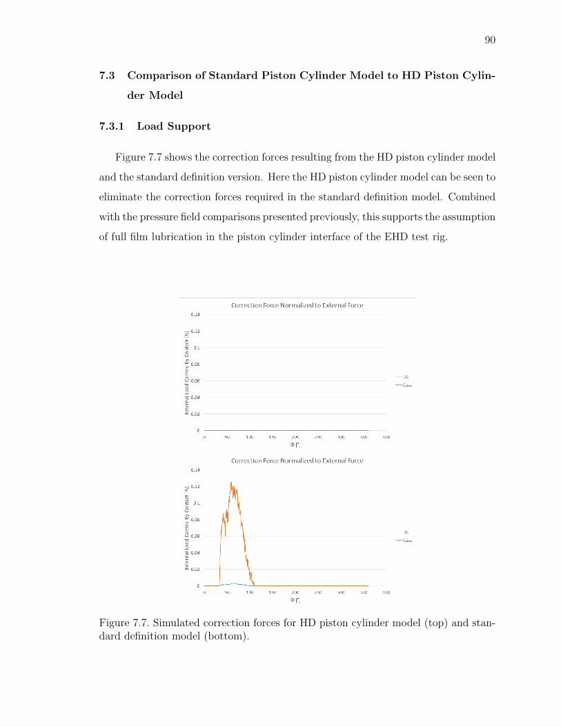
90

7.3 Comparison of Standard Piston Cylinder Model to HD Piston Cylin-

der Model

7.3.1 Load Support

Figure 7.7 shows the correction forces resulting from the HD piston cylinder model

and the standard definition version. Here the HD piston cylinder model can be seen to

eliminate the correction forces required in the standard definition model. Combined

with the pressure field comparisons presented previously, this supports the assumption

of full film lubrication in the piston cylinder interface of the EHD test rig.

Figure 7.7. Simulated correction forces for HD piston cylinder model (top) and stan-dard definition model (bottom).

91

7.3.2 Friction Forces

Predicted axial friction forces for both the HD and standard definition piston

cylinder models are shown in Figure 7.8. The standard definition model predicts

higher Couette friction while correction forces are present due to the reduced film

thickness in the collapsed regions.

Figure 7.8. Simulated axial friction forces for HD piston cylinder model and standarddefinition model.

92

7.3.3 Energy Dissipation

Figure 7.9 compares the power loss predictions of the HD piston cylinder model

and the standard definition model. Overall predicted power loss from the HD piston

cylinder model is reduced by 15% compared to the standard definition model. Two

factors contribute to this difference. First, the lower predicted friction discussed

previously leads to lower mechanical power loss. Second, the volumetric power loss

is reduced over much of the high pressure stroke.

Figure 7.9. Simulated power losses for HD piston cylinder model and standard defi-nition model.

93

7.3.4 Leakage Flow

The decreased volumetric power loss is the result of decreased leakage flow as

shown in Figure 7.10.

Figure 7.10. Simulated leakage flow for HD piston cylinder model and standard defi-nition model.

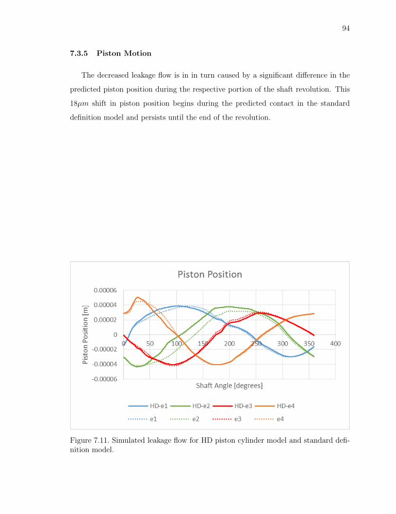
94

7.3.5 Piston Motion

The decreased leakage flow is in in turn caused by a significant difference in the

predicted piston position during the respective portion of the shaft revolution. This

18µm shift in piston position begins during the predicted contact in the standard

definition model and persists until the end of the revolution.

Figure 7.11. Simulated leakage flow for HD piston cylinder model and standard defi-nition model.

95

7.3.6 Film Thickness

Figure 7.12 shows the film thickness predicted by the HD piston cylinder model

and the standard definition model at 90◦ shaft angle. The primary leakage flow

path can be seen following the path of high film thickness from the left side of the

plot to the right. This flow path experiences significantly lower film thicknesses in

the HD piston cylinder model’s prediction, leading to the lower predicted leakages.

Figure 7.13 shows the difference between the film thickness predictions of the HD

piston cylinder model and the standard definition model. The impact of the 18µm

difference in piston position is visible in the different film thicknesses. Note however

that the difference of film thickness in the critical areas of low film thickness are

minimal.

96

Figure 7.12. Simulated film thickness at 90◦ for HD piston cylinder model (top) andstandard definition model (bottom).

97

Figure 7.13. Absolute difference in simulated film thickness between HD piston cylin-der model and standard definition model.

98

8. CONTRIBUTIONS

A novel piston cylinder interface model is introduced that advances the understanding

of the tribological effects in play at the piston cylinder interface. Model advances

resulting from this work are:

• Physical effects have been added to the piston cylinder model Reynolds Equa-

tion:

– Elastohydrodynamic (EHD) squeeze is added.

– Accurate surface velocities are considered with respect to translational

squeeze.

– Compressible flow is considered.

• Two-dimensional surface wear profiles are defined and implemented.

• Measured surface profiles are implemented for all simulated operating condi-

tions.

• Methods for preventing fluid film collapse and ensuring force balance are intro-

duced.

• Finite Element Method (FEM) solver implemented for solid body thermal anal-

ysis.

The improved standard piston cylinder model is compared against measurements

made using an improved Tribo test rig. The reconfigured Tribo test rig exhibits an

improved signal to noise ratio and a more stable and controllable inlet fluid temper-

ature. Comparison between simulation results and measured friction profiles shows

99

good agreement across the limited range of operating conditions available for com-

parison.

A novel high definition lubrication model is introduced and developed. The high

definition model refines areas of collapsed fluid film predicted by the standard piston

cylinder model to investigate the impact of a finer grid spacing on improving load

support. Advances resulting from this work are:

• An adaptive multigrid solver is implemented, with refinement based on film

thickness.

• A linear half-space deformation model is implemented for high-resolution defor-

mation calculations.

• A new fluid model extending to 3000bar is developed for the fluid used in

measurement.

Results of the high definition lubrication model suggest that sufficient load support

can be calculated in order to prevent fluid film collapse, leading to the integration

of the high definition pressure calculations with the standard piston cylinder model.

This high definition piston cylinder model is used to simulate the operating condition

of EHD Test Rig measurements made by Pelosi [15]. Advances resulting from this

work are:

• Development of a physics based method for calculating the motion of the piston

resulting from force balance.

• Improved understanding and modeling of the impact of film thickness on mea-

sured pressure fields in the EHD test rig.

Results comparison with measurement shows a good match with both temperature

and pressure fields, and indicates full film lubrication prevails in the lubricating film

between piston and cylinder throughout steady state operation.

LIST OF REFERENCES

100

LIST OF REFERENCES

[1] A. Yamaguchi. Motion of pistons in piston-type hydraulic machines. Bulletin ofthe JSME, 19(130), 4 1976.

[2] A. Yamaguchi. Motion of the piston in piston pumps and motors: The case ofmetallic contact. JSME International Journal, Series III, 33(4):627 – 633, 1990.

[3] K. Sadashivappa, M. Singaperumal, and K. Narayanasamy. On the efficiency ofthe axial piston motor considering piston form deviations. 6:283–301, 04 1996.

[4] S. Gels and H. Murrenhoff. Simulation of the lubricating film between contouredpiston and cylinder. International Journal of Fluid Power, 11(2):15–24, 2010.

[5] Sushil Kumar and J Bergada. The effect of piston grooves performance in anaxial piston pumps via cfd analysis. 66:168–179, 01 2013.

[6] P. Agarwal, A. Vacca, K. Wang, K. Sun Kim, and T. Kim. An analysis oflubricating gap flow in radial piston machines. 7:524–534, 05 2014.

[7] A. Kuzmin, V. Popov, and S. Stazhkov. Hydrodynamic processes in pistonboreinterface of axial piston swash plate machine. In 28th DAAAM InternationalSymposium on Intelligent Manufacturing and Automation, pages 0621–0626, 012017. ISBN 9783902734112.

[8] Y. Fang and M. Shirakashi. Mixed lubrication characteristics between the pistonand cylinder in hydraulic piston pump-motor. ASME Journal of Tribology, 117:80 – 85, 1 1995.

[9] A. Fatemi, A. Wohlers, and H. Murrenhoff. Simulation of elastohydrodynamiccontact between piston and cylinder in axial piston pumps. In 6th InternationalFluid Power Conference, Dresden, 2008.

[10] M. Berge. An Investigation of Viscous Flow in Lubricating Gaps. PhD thesis,SVST, Bratislava, Czechoslovakia, 1983. In Slovak, now Ivantysynova, M.

[11] U. Wieczorek. Ein Simulationsmodell zur Beschreibung der Spaltstromung inAxialkolbenmaschinen der Schragscheibenbauart. Number 443 in 7. VDI, Dussel-dorf, 2003.

[12] M. Ivantysynova and C. Huang. Investigation of the gap flow in displacementmachines considering elastohydrodynamic effect. In 5th JFPS International Sym-posium on Fluid Power, pages 219 – 229, Nara, Japan, 2002.

101

[13] M. Pelosi and M. Ivantysynova. A novel thermal model for the piston/cylinderinterface of piston machines. In Bath ASME Symposium on Fluid Power andMotion Control (FPMC2009), 2009.

[14] M. Pelosi and M. Ivantysynova. Surface deformation enables high pressure op-eration of axial piston pumps. In ASME/Bath Symposium on Fluid Power andMotion Control, Arlington, VA, USA, 2011.

[15] M. Pelosi. An Investigation on the Fluid-Structure Interaction of Piston/CylinderInterface. PhD thesis, Purdue University, West Lafayette, 5 2012.

[16] J. R. Dowd and F. T. Barwell. Tribological interaction between piston andcylinder of a model high pressure hydraulic pump. A S L E Transactions, 18(1):21 – 30, 1975.

[17] C. J. Hooke and Y. P. Kakoullis. The effects of centrifugal load and ball frictionon the lubrication of slippers in axial piston pumps. In Papers Presented at theSixth International Fluid Power Symposium, pages 179 – 181, St. John’s College,Cambridge, England, 4 1981.

[18] N. D. Manring. Friction forces within the cylinder bores of swash-plate type axial-piston pumps and motors. ASME Journal of Dynamic Systems, Measurement,and Control, 121:531 – 537, 9 1999.

[19] K. Tanaka, K. Kyogoku, and T. Nakahara. Lubrication characteristics on slidingsurfaces between piston and cylinder in a piston pump and motor (effects ofrunning-in, profile of piston top and stiffness). JSME International Journal,Series C, 42(4):1031 – 1040, 1999.

[20] M. B. Treuhaft, S. A. Timmons, and G. R. Eberle. Wear measurement of a largehydraulic fluid power pump using radioactive tracer wear technology. In ASMEInternational Mechanical Engineering Congress and Exposition, pages 55 – 64,Washington, D.C., 11 2003.

[21] R. Lasaar and M. Ivantysynova. A new test rig for measuring friction forcesin swash plate type axial piston pumps. In Proc. 1st Bratislavian Fluid PowerSymposium, pages 59 – 69, Casta-Pila, Slovakia, 1998.

[22] H. Everth. Development of a model pump for measurement of dynamic pressurefields between piston and cylinder to proof ehd simulation model. Master’s thesis,Technical University Hamburg-Harburg, Hamburg, 10 2003.

[23] H. Everth. Development of measurement system for pressure and temperaturefield measurements using a single piston-cylinder test pump. Master’s thesis,Technical University Hamburg-Harburg, Hamburg, 12 2003.

[24] D. Dowson and G. R. Higginson. A numerical solution to the elasto-hydrodynamic problem. Journal of Mechanical Engineering Science, 1(1):6 –15, 1959.

[25] C. J. A. Roelands. Correlational aspects of the viscosity-temperature-pressurerelationship of lubricating oils. PhD thesis, Delft University of Technology, 41966. uuid:1fb56839-9589-4ffb-98aa-4a20968d1f90.

102

[26] H. S. Cheng. A numerical solution of the elastohydrodynamic film thickness inan elliptical contact. Journal of Lubrication Technology, 92(1):155 – 162, 1970.

[27] C. Taylor and J. F. O’Callaghan. A numerical solution of the elastohydrodynamiclubrication problem using finite elements. Journal of Mechanical Science, 14:229– 237, 1972.

[28] A. Brandt. Multi-level adaptive technique (mlat) for fast numerical solution toboundary value problems. In Proc. of the 3rd International Conference on Nu-merical Methods in Fluid Mechanics, Lecture Notes in Physics, volume 18/1973,pages 82 – 89, 1973.

[29] A. Brandt. Multi-level adaptive solutions to boundary-value problems. Mathe-matics of Computation, 31(138):333 – 390, 1977.

[30] B. J. Hamrock and D. Dowson. Numerical evaluation of surface deformation ofelastic solids subjected to hertzian contact stress. Tech Note D-7774, NASA,1974.

[31] D. E. Brewe, B. J. Hamrock, and C. M. Taylor. Effect of geometry on hydrody-namic film thickness. ASME Journal of Lubrication Technology, 101:231 – 237,4 1979.

[32] L. G. Houpert and B. J. Hamrock. Fast approach for calculating film thicknessesand pressures in elastohydrodynamically lubricated contacts at high loads. Jour-nal of Tribology, 108(3):411 – 420, 1986.

[33] A. A. Lubrecht, W. E. Ten Napel, and R. Bosma. Multigrid, and alternativemethod for calculating film thickness and pressure profiles in elastohydrodynam-ically lubricated line contacts. Trans. ASME, Journal of Tribology, 108:551 –556, 1986.

[34] K. Kim and F. Sadeghi. Three-dimensional temperature distribution in ehdlubrication: Part i - circular contact. ASME Journal of Tribology, 114:32–41,1992.

[35] K. Kim and F. Sadeghi. Three-dimensional temperature distribution in ehdlubrication: Part ii - point contact and numerical formulation. ASME Journalof Tribology, 115:36 – 45, 1993.

[36] Y. Z. Hu and D. Zhu. A full numerical solution to the mixed lubrication in pointcontacts. ASME Journal of Tribology, 122:1 – 9, 1 2000.

[37] C. E. Goodyer. Adaptive Numerical Methods for Elastohydrodynamic Lubrica-tion. PhD thesis, University of Leeds, Leeds, UK, 5 2001.

[38] W. W. Habchi. Coupling strategies for finite element modeling of thermal elas-tohydrodynamic lubrication problems. ASME Journal of Tribolology, 139(4),2017.

[39] B. J. Hamrock, S. R. Schmid, and B. O. Jacobson. Fundamentals of Fluid FilmLubrication. Marcel Dekker, Inc., New York, 3 edition, 2004. ISBN 0-8247-5371-2.

103

[40] M. Zecchi. A Novel Fluid Structure Interaction and Thermal Model to Predictthe Cylinder Block/Valve Plate Interface Performance in Swash Plate Type AxialPiston Machines. PhD thesis, Purdue University, West Lafayette, 12 2013.

[41] L. Shang. A Path Toward an Effective Scaling Approach for Axial Piston Ma-chine. PhD thesis, Purdue University, West Lafayette, IN, 2018. Unpublished attime of writing.

VITA

104

VITA

Daniel Mizell was born in 1989 in Southeast Michigan. He earned his B.S. in

Mechanical Engineering in 2011 at Michigan Technological University in Houghton,

MI. In August 2011, Dan came to Purdue to join the team at the Maha Fluid Power

Research Center. There, he earned his M.S. in Mechanical Engineering in 2014 while

working toward his Direct PhD. Dan’s research activities focus on advanced modeling

of the piston cylinder interface of swash plate type axial piston machines.

Dan met his wife Ashby while studying at Michigan Technological University, and

they were married in 2011. Their son Troy was born in 2013.

A Study of the Piston Cylinder Interface of Axial Piston Machines

Documents