A Study of Permutation Groups and Coherent Configurations

A study of permutation groups and coherent configurations

by

John Herbert Batchelor

A Creative Component submitted to the graduate faculty

in partial fulfillment of the requirements for the degree of

MASTER OF SCIENCE

Major: Mathematics

Program of Study Committee:Sung-Yell Song, Major Professor

Irvin HentzelJue Yan

Iowa State University

Ames, Iowa

2009

Copyright c© John Herbert Batchelor, 2009. All rights reserved.

ii

TABLE OF CONTENTS

ABSTRACT . . . . . . . . . . . . . . . . . . . . . . . . . . . . . . . . . . . . . . . iii

CHAPTER 1. HISTORICAL BACKGROUND . . . . . . . . . . . . . . . . . 1

1.1 Early Historical Background . . . . . . . . . . . . . . . . . . . . . . . . . . . . . 1

1.2 Resolvent Polynomials . . . . . . . . . . . . . . . . . . . . . . . . . . . . . . . . 2

1.3 More Recent Developments . . . . . . . . . . . . . . . . . . . . . . . . . . . . . 3

1.3.1 Galois Groups . . . . . . . . . . . . . . . . . . . . . . . . . . . . . . . . 3

1.3.2 Additional Facts . . . . . . . . . . . . . . . . . . . . . . . . . . . . . . . 4

CHAPTER 2. SHARPLY 2-TRANSITIVE GROUPS . . . . . . . . . . . . . 6

2.1 Notation and Basic Definitions . . . . . . . . . . . . . . . . . . . . . . . . . . . 6

2.2 Coset Spaces . . . . . . . . . . . . . . . . . . . . . . . . . . . . . . . . . . . . . 11

2.3 Characterization of Sharply 2-Transitive Permutation Groups . . . . . . . . . . 12

CHAPTER 3. COHERENT CONFIGURATIONS . . . . . . . . . . . . . . . 18

3.1 Coherent Configurations and Basis Algebras . . . . . . . . . . . . . . . . . . . . 18

3.2 Association Schemes . . . . . . . . . . . . . . . . . . . . . . . . . . . . . . . . . 19

3.3 Schur Rings . . . . . . . . . . . . . . . . . . . . . . . . . . . . . . . . . . . . . . 22

3.4 Construction of Non-Symmetric Commutative Association Schemes Using Schur

Rings . . . . . . . . . . . . . . . . . . . . . . . . . . . . . . . . . . . . . . . . . 24

3.5 Permutation Representations and Centralizer Algebras . . . . . . . . . . . . . . 30

3.6 Character Theory . . . . . . . . . . . . . . . . . . . . . . . . . . . . . . . . . . . 30

BIBLIOGRAPHY . . . . . . . . . . . . . . . . . . . . . . . . . . . . . . . . . . . 33

ACKNOWLEDGEMENTS . . . . . . . . . . . . . . . . . . . . . . . . . . . . . . 34

iii

ABSTRACT

Permutation groups have fascinated mathematicians for hundreds of years; they are a

central topic in abstract algebra. In this creative component, we will discuss permutation

groups and their actions. We will begin by covering the historical background of the study

of permutation groups, from Lagrange’s results to more recent developments such as Galois

groups. Next, we will discuss basic concepts and state definitions relevant to permutation group

theory. This paper will also include some more advanced topics such as coherent configurations

and association schemes. We will discuss Schur rings and permutation representations and

conclude with a brief introduction to character theory.

1

CHAPTER 1. HISTORICAL BACKGROUND

In this chapter, we will discuss the historical background relevant to the study of permuta-

tion groups, as well as some of the questions that have motivated the study of this topic. The

purpose of this chapter is to provide a brief survey of the history of permutation group theory,

with emphasis given to topics that will be covered later in this paper. Note that this chapter

includes some references to terminology that will be defined in Chapter 2 and Chapter 3.

1.1 Early Historical Background

Permutation groups were one of the first topics that mathematicians studied in group

theory [5]. In 1770, Lagrange discussed permutations when he was studying algebraic solutions

to polynomial equations. This problem involves determining the roots of a given polynomial in

terms of an algebraic formula involving the polynomial’s coefficients. Mathematicians wanted

to derive formulas to construct roots using only addition, subtraction, multiplication, division,

and extraction of kth roots (k ∈ N). This technique is called solution by radicals.

Example 1.1.1. The most familiar example of solution by radicals is the quadratic formula.

Given a polynomial equation of the form ax2 + bx+ c = 0, the roots are given by

x =−b±

√b2 − 4ac

2a.

Similar formulas exist for the solution of cubic and quartic (degree 4) equations. However, no

such formula exists for quintic (degree 5) polynomials.

Lagrange explained that these algorithms depended on finding resolvent polynomials, which

are discussed in the next section. The roots of the resolvent polynomials are used to determine

the roots of the original polynomials.

2

1.2 Resolvent Polynomials

Consider a set A = X1, X2, · · · , Xn containing n variables. The symmetric group Sn acts

on A by permuting the subscripts of the variables. This action of Sn on A can be extended to

an action on the set of all polynomials in the variables X1, X2, · · · , Xn.

Example 1.2.1. Let z =(1 2)(

3 4)∈ S4, and define Φ = X1X3 − X2X4. Then Φz =

X2X4 −X1X3 = −Φ. The orbit of Φ under S4 is given by

O = X1X3−X2X4, X2X4−X1X3, X1X2−X3X4, X3X4−X1X2, X1X4−X2X3, X2X3−X1X4.

Lagrange called these six polynomials the values of Φ. By the orbit-stabilizer property (The-

orem 2.1.1), the stabilizer of Φ in S4 has order 4!6 = 24

6 = 4.

Definition 1.2.2. Let Φ be a polynomial inX1, X2, · · · , Xn with k values Φ = Φ(1),Φ(2), · · · ,Φ(k).

The resolvent h is a polynomial in X1, X2, · · · , Xn, Z defined as follows.

h(Z) =k∏i=1

(Z − Φ(i)

)=

k∑j=0

hj(X1, X2, · · · , Xn

)Zj .

Note that the values Φ(1),Φ(2), · · · ,Φ(k) form an orbit under Sn, and so the polynomial h

is invariant under arbitrary permutations of X1, X2, · · · , Xn. Therefore, each polynomial

hj(X1, X2, · · · , Xn) is symmetric in X1, X2, · · · , Xn, and we can express them as polynomials

in the elementary symmetric functions of X1, X2, · · · , Xn.

Example 1.2.3. Let f(x) be a polynomial of degree n with roots r1, r2, · · · , rn. Substitute

r1, r2, · · · , rn for X1, X2, · · · , Xn in the expression for h(Z) to obtain the following polynomial

in Z:

p(Z) =k∑j=0

hj(r1, r2, · · · , rn)Zj .

We can determine the coefficients of p(Z) from the coefficients of f(x). By choosing Φ carefully,

we may be able to solve the polynomial h(Z) and determine the roots r1, r2, · · · , rn from the

roots Φ(1)(r1, r2, · · · , rn),Φ(2)(r1, r2, · · · , rn), · · · ,Φ(k)(r1, r2, · · · , rn) of h(Z).

Paolo Ruffini and Niels Abel used the method of resolvents to prove that solution by radicals

cannot be used to solve the general equation of degree 5 or greater.

3

1.3 More Recent Developments

We close this chapter with a summary of some more recent results in permutation group

theory.

1.3.1 Galois Groups

Galois considered the question of whether a given polynomial could be solved using radicals.

In 1830, he made a major discovery. For each polynomial f(x) with distinct roots r1, r2, · · · , rn,

there exists an associated permutation group on the set of roots. Mathematicians call this

group the Galois group of f(x) [8]. The structure of the Galois group determines whether f(x)

can be solved by radicals. Note that the following definition from [5] uses modern field theory

terminology.

Definition 1.3.1. Consider a field K that contains the coefficients of f(x). Adjoin the roots to

obtain a splitting field L. The field automorphisms of L that fix every element of K constitute

a finite group G. This group acts on the set of roots. The Galois group of f(x) is the set of

permutations of r1, r2, · · · , rn induced by the elements of G.

Next, we will discuss the relationship between Galois groups and Lagrange resolvents. Let Φ

be a polynomial over K in n variables such that each of the roots r1, r2, · · · , rn of f(x) can be

expressed as a polynomial over K in t, where t = Φ(r1, r2, · · · , rn). That is, K(r1, r2, · · · , rn) =

K(t). For each x ∈ Sn, let tx = Φ(r1′ , r2′ , · · · , rn′), where i′ = ix for all i ∈ 1, 2, · · · , n. Now

define the resolvent g(Z) as follows:

g(Z) =∏x∈Sn

(Z − tx).

Note that g is a polynomial of degree n! over K. Factor g(Z) over K to obtain an irreducible

factor, say g1(Z), that has t as a root. Now let G denote the Galois group for f(x). Then

g1(Z) has degree |G|, and the set of roots of g1(Z) is given by tx : x ∈ G.

4

1.3.2 Additional Facts

Several other mathematicians have made major contributions to the development of per-

mutation group theory. By the middle of the 1800s, mathematicians had developed a solid

theory of permutation groups. In 1870, Camille Jordan published Traite des Substitutions

et des Equations Algebriques. This book was based on papers written by Galois in 1832. It

was the first text on the topic of permutation groups, and it was reprinted in 1957. William

Burnside published important research on 2-transitive permutation groups. In 1897, he pub-

lished his book, Theory of Groups of Finite Order. It was the first text on finite group theory

written in English [4]. Burnside studied the problem of finding invariants of finite groups. He

was particularly interested in the icosahedral group in four variables. He proved the following

theorem on transitive permutation groups.

Theorem 1.3.2. Let G be a transitive permutation group on p symbols, where p is prime.

Then G is either solvable or 2-transitive.

Ferdinand Frobenius also contributed to the advancing study of permutation groups. In 1900,

he published research on the use of permutation characters to compute the characters of the

symmetric group Sn. He served as Issai Schur’s advisor, and he proved the following important

result.

Theorem 1.3.3. Suppose that G is a transitive permutation group that acts on a set X con-

taining n elements. Assume that no non-identity element of G fixes more than one element of

X. Then there are exactly n − 1 elements of G that have no fixed points in X. These n − 1

elements, along with the identity, constitute a normal subgroup of G.

Frobenius introduced the concept of Frobenius groups, a special kind of transitive group. A

Frobenius group is defined as a transitive permutation group that is not regular (cf. Definition

2.1.9) but has the property that only the identity has two or more fixed points [5]. Frobenius,

Zassenhaus, and J.G. Thompson proved important results about the structure of finite Frobe-

nius groups. A 2-transitive Frobenius group is often called a sharply 2-transitive group (cf.

Section 2.3). Examples of Frobenius groups include the dihedral groups of order 2q, where q

5

is odd [4]. In 1902, Frobenius proved that in a Frobenius group G of degree n, the identity

together with the elements of degree n constitute a regular group which is a characteristic

subgroup of G.

Issai Schur specialized in representation theory of finite groups. He served as a mentor to

Helmut Wielandt, who proved numerous results in permutation group theory [4]. In 1908, he

published a new proof of Theorem 1.3.2. Schur referred to this theorem as “one of the most

important new results in finite group theory.” Schur expanded on some of Frobenius’ results

concerning characters and representations of finite groups. His fundamental idea was to regard

group elements as “points,” instead of using arbitrary objects or the integers 1, 2, · · · , n [10].

Wielandt, Bercov, and Kochendorffer also proved important results concerning Schur rings.

Coherent configurations, which are discussed in detail in Chapter 3, were introduced by Donald

Higman in his 1967 paper, “Intersection matrices for finite permutation groups.” Higman

defined the concept of structure numbers, denoted phij , which are described in Section 3.2.

R.C. Bose and K.R. Nair discussed association schemes in their paper, “Partially balanced

incomplete block design.” The study of association schemes grew from the fields of statistics

and experimental design. Bose defined an association scheme as a coherent configuration

(Ω,R) such that all relations in R are symmetric. Bose and D.M. Mesner described the basis

algebra of an association scheme in 1959; this algebra is now called the Bose-Mesner algebra

[3]. In 1973, Philippe Delsarte published his paper, “An algebraic approach to the association

schemes of coding theory,” in which he proved several results concerning association schemes.

Delsarte also developed the theory of duality for association schemes that admit a regular

abelian automorphism group. Association schemes are discussed in detail in Section 3.2.

6

CHAPTER 2. SHARPLY 2-TRANSITIVE GROUPS

In this chapter, we will discuss the basic concepts and definitions relevant to permutation

groups. We shall conform to the standard notation used in Wielandt’s book [10] and Cameron’s

book [3].

2.1 Notation and Basic Definitions

In this chapter we will study permutations on a finite set Ω. Let Ω be a finite set of

arbitrary elements called points and denoted by lower case Greek letters such as α, β, γ, etc.

Upper case Greek letters such as Γ,∆ are used to denote subsets of Ω. For a subset ∆ ⊆ Ω, let

|∆| denote the number of points in ∆, or the cardinality of ∆. We will generally use positive

integers to denote the points of Ω, as follows: Ω = 1, 2, · · · , n. A permutation on Ω is a

one-to-one mapping of Ω onto Ω. The image of a point α ∈ Ω under a permutation g is denoted

αg. Using this notation for the image, we express a permutation g as follows:

g =

1 2 · · · n

1g 2g · · · ng

=

α

αg

The product of two permutations g and h on Ω, denoted gh, is defined as follows:

α(gh) = (αg)h

The identity permutation, denoted 1, leaves all points of Ω fixed. The permutation inverse to

g, written g−1, is characterized by the following property: If g maps α to β, then g−1 maps β

to α. Given a set Ω, the symmetric group SΩ is the set of all permutations on Ω. The group

operation for SΩ is composition, denoted gh and defined by (α)gh = (αg)h, for all α ∈ Ω

7

and all g, h ∈ SΩ. When |Ω| = n, we often write Sn to denote the symmetric group [7]. A

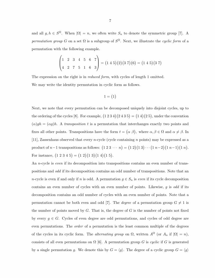
permutation group G on a set Ω is a subgroup of SΩ. Next, we illustrate the cyclic form of a

permutation with the following example.1 2 3 4 5 6 7

4 2 7 5 1 6 3

=(1 4 5

)(2)(

3 7)(

6)

=(1 4 5

)(3 7)

The expression on the right is in reduced form, with cycles of length 1 omitted.

We may write the identity permutation in cyclic form as follows.

1 =(1)

Next, we note that every permutation can be decomposed uniquely into disjoint cycles, up to

the ordering of the cycles [8]. For example,(1 2 3 4

)(2 4 3 5

)=(1 4)(

2 5), under the convention

(α)gh = (αg)h. A transposition t is a permutation that interchanges exactly two points and

fixes all other points. Transpositions have the form t =(α β

), where α, β ∈ Ω and α 6= β. In

[11], Zassenhaus observed that every n-cycle (cycle containing n points) may be expressed as a

product of n−1 transpositions as follows:(1 2 3 · · · n

)=(1 2)(

1 3)· · ·(1 n−2

)(1 n−1

)(1 n).

For instance,(1 2 3 4 5

)=(1 2)(

1 3)(

1 4)(

1 5).

An n-cycle is even if its decomposition into transpositions contains an even number of trans-

positions and odd if its decomposition contains an odd number of transpositions. Note that an

n-cycle is even if and only if n is odd. A permutation g ∈ Sn is even if its cycle decomposition

contains an even number of cycles with an even number of points. Likewise, g is odd if its

decomposition contains an odd number of cycles with an even number of points. Note that a

permutation cannot be both even and odd [7]. The degree of a permutation group G 6= 1 is

the number of points moved by G. That is, the degree of G is the number of points not fixed

by every g ∈ G. Cycles of even degree are odd permutations, and cycles of odd degree are

even permutations. The order of a permutation is the least common multiple of the degrees

of the cycles in its cyclic form. The alternating group on Ω, written AΩ (or An if |Ω| = n),

consists of all even permutations on Ω [6]. A permutation group G is cyclic if G is generated

by a single permutation g. We denote this by G = 〈g〉. The degree of a cyclic group G = 〈g〉

8

is the degree of the permutation g. Let G be a group acting on a set Ω, and let α ∈ Ω. The

set αG = αg : g ∈ G is called the orbit of G containing α. The stabilizer of α in G is the

set Gα = g ∈ G : αg = α. If G ≤ SΩ and ∆ ⊆ Ω, the stabilizer of ∆ in G is the set

G∆ = g ∈ G : αg = α, for all α ∈ ∆. If ∆ = α, then G∆ = Gα. A permutation group G

is transitive if for all α, β ∈ Ω, there exists g ∈ G such that αg = β. So the action of G on Ω is

transitive if there is only one orbit. The following result is called the orbit-stabilizer property.

Theorem 2.1.1. Let G be a finite permutation group on Ω. Then |G| = |Gα| · |αG| for all

α ∈ Ω.

Proof. Let αG = β1, β2, · · · , βr. Then there exist g1, g2, · · · , gr ∈ G such that αgi = βi for

i = 1, 2, · · · , r. Let P = g1, g2, · · · , gr. Then |P | = |αG|. It is sufficient to show that for

any g ∈ G, g can be expressed in exactly one way as the product of a permutation in P and

a permutation in Gα, so that |G| = |P | · |Gα| which will complete the proof. Given g ∈ G,

αg = βk for some k ∈ 1, 2, · · · , r. This means that αg = αgk, so gg−1k leaves α fixed. That is,

gg−1k ∈ Gα. But (gg−1

k ) · gk = g, so g is the product of a permutation in Gα and a permutation

in P . Now suppose that g can be written in two ways as such a product: g = hgk = fgl for

h, f ∈ Gα. Then αhgk = βk and αfgl = βl. This forces βk = βl, and so k = l. Therefore,

g = h · gk = f · gk and h = f .

The following orbit-counting lemma is often called “Burnside’s Lemma,” but Burnside was not

the first to prove it. It was known to earlier mathematicians including Frobenius. Let ψ(g)

denote the number of points of Ω that are fixed by the element g ∈ G. That is, ψ(1) = |Ω|.

Lemma 2.1.2. Let G be a permutation group on a finite set Ω. Then the number of orbits of

G on Ω is equal to the average number of fixed points of an element of G. That is, the number

of orbits of G is1|G|

∑g∈G

ψ(g).

Proof. Note that ∑g∈G

ψ(g) =∑α∈Ω

|Gα| = |(g, α) : αg = α|.

9

By the orbit-stabilizer property,

1|G|

∑g∈G

ψ(g) =1|G|

∑α∈Ω

|Gα| =∑α∈Ω

|Gα||G|

=∑α∈Ω

1|αG|

.

The proof follows from the fact that the sum on the right-hand side indicates the number of

orbits.

Lemma 2.1.3. Let G be a transitive permutation group on the finite set Ω with |Ω| > 1.

Then there exists g ∈ G such that αg 6= α, for all α ∈ Ω. (Such an element g is called

fixed-point-free.)

Proof. Note that this result follows from Burnside’s Lemma, which states that the number of

orbits of G on Ω equals the average number of fixed points of an element of G. The average

number of fixed points is 1, and the identity fixes more than one point. So there exists some

element g ∈ G that fixes no point. An alternate proof involving maximal subgroups is given

below.

We are given that G is a transitive permutation group on a finite set Ω, where |Ω| ≥ 2. We

must show that there exists some g ∈ G such that αg 6= α, for all α ∈ Ω. First, we claim that

if g ∈ G,α ∈ Ω, and αg = β, then g−1Gαg ⊆ Gβ. To see this, suppose that g′ ∈ g−1Gαg.

Then g′ = g−1hg, for some h ∈ Gα. Note that αh = α (since h ∈ Gα). So

βg′ = (αg)(g−1hg) = α(gg−1)hg = (αh)g = αg = β.

That is, βg′ = β. Hence, g′ ∈ Gβ. Therefore, g−1Gαg ⊆ Gβ.

Our second claim is that ⋃g∈G

gGαg−1

for α ∈ Ω is a proper subset of G. To show this, let M be a maximal subgroup containing Gα

in G. Consider the conjugation action of G on the set P(G) of all subgroups of G. We observe

that the point stabilizer GM = M since GM = g ∈ G : gMg−1 = M = NG(M) and M is a

maximal subgroup of G. This means that the size of the orbit containing M is |G||M | by Theorem

2.1.1 (the orbit-stabilizer property). Since each element of the orbit MG is a subgroup of G of

10

the form gMg−1 for some g ∈ G \M , |gMg−1| = |M |. As all subgroups contain the identity

element of G, we have∣∣∣∣⋃g∈G

gGαg−1

∣∣∣∣ ≤ ∣∣∣∣⋃g∈G

gMg−1

∣∣∣∣ ≤ (|M | − 1) |G||M |

< |G|,

as desired.

We now prove the conclusion by way of contradiction. Suppose that for all g ∈ G, there is an

element α ∈ Ω such that αg = α. Let |Ω| = n (n ≥ 2, finite), and denote the elements of Ω by

α1, α2, · · · , αn. By transitivity, for all αi, αj ∈ Ω, there exists gij ∈ G such that αigij = αj . By

our assumption, for each gij ∈ G, there is some element αk ∈ Ω such that αkgij = αk. Hence,

gij ∈ G(αk). So G = G(α1) ∪G(α2) ∪ · · · ∪G(αn). By the first claim above,

G(α1) ∪G(α2) ∪ · · · ∪G(αn) =⋃g∈G

gG(α1)g−1;

so

G =⋃g∈G

gG(α1)g−1.

This is a contradiction to the second claim, since G(α1) is a proper subgroup of G. This

completes the proof.

Definition 2.1.4. Let k ∈ N be such that k < |Ω|. A permutation group G is k-transitive on

Ω if G acts transitively on the set of k-tuples of distinct elements, where the componentwise

action is defined by (α1, α2, · · · , αk)g = (α1g, α2g, · · · , αkg). In other words, G is k-transitive

if for every two ordered k-tuples (α1, α2, · · · , αk) and (β1, β2, · · · , βk) consisting of distinct

points of Ω, there exists g ∈ G such that αig = βi for all i ∈ 1, 2, · · · , k. We say that G is

sharply k-transitive if there exists exactly one such g ∈ G for every two such k-tuples. Note

that if k ≥ 2, then G is k-transitive on Ω if and only if both of the following conditions hold:

1. G is transitive on Ω.

2. Gα is (k − 1)-transitive on Ω \ α.

In some texts such as [10], this concept is called k-fold transitivity.

11

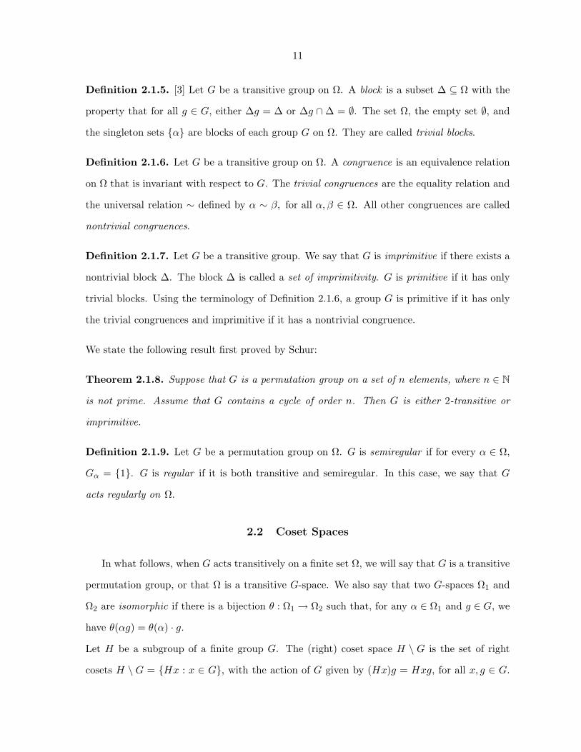
Definition 2.1.5. [3] Let G be a transitive group on Ω. A block is a subset ∆ ⊆ Ω with the

property that for all g ∈ G, either ∆g = ∆ or ∆g ∩∆ = ∅. The set Ω, the empty set ∅, and

the singleton sets α are blocks of each group G on Ω. They are called trivial blocks.

Definition 2.1.6. Let G be a transitive group on Ω. A congruence is an equivalence relation

on Ω that is invariant with respect to G. The trivial congruences are the equality relation and

the universal relation ∼ defined by α ∼ β, for all α, β ∈ Ω. All other congruences are called

nontrivial congruences.

Definition 2.1.7. Let G be a transitive group. We say that G is imprimitive if there exists a

nontrivial block ∆. The block ∆ is called a set of imprimitivity. G is primitive if it has only

trivial blocks. Using the terminology of Definition 2.1.6, a group G is primitive if it has only

the trivial congruences and imprimitive if it has a nontrivial congruence.

We state the following result first proved by Schur:

Theorem 2.1.8. Suppose that G is a permutation group on a set of n elements, where n ∈ N

is not prime. Assume that G contains a cycle of order n. Then G is either 2-transitive or

imprimitive.

Definition 2.1.9. Let G be a permutation group on Ω. G is semiregular if for every α ∈ Ω,

Gα = 1. G is regular if it is both transitive and semiregular. In this case, we say that G

acts regularly on Ω.

2.2 Coset Spaces

In what follows, when G acts transitively on a finite set Ω, we will say that G is a transitive

permutation group, or that Ω is a transitive G-space. We also say that two G-spaces Ω1 and

Ω2 are isomorphic if there is a bijection θ : Ω1 → Ω2 such that, for any α ∈ Ω1 and g ∈ G, we

have θ(αg) = θ(α) · g.

Let H be a subgroup of a finite group G. The (right) coset space H \ G is the set of right

cosets H \ G = Hx : x ∈ G, with the action of G given by (Hx)g = Hxg, for all x, g ∈ G.

12

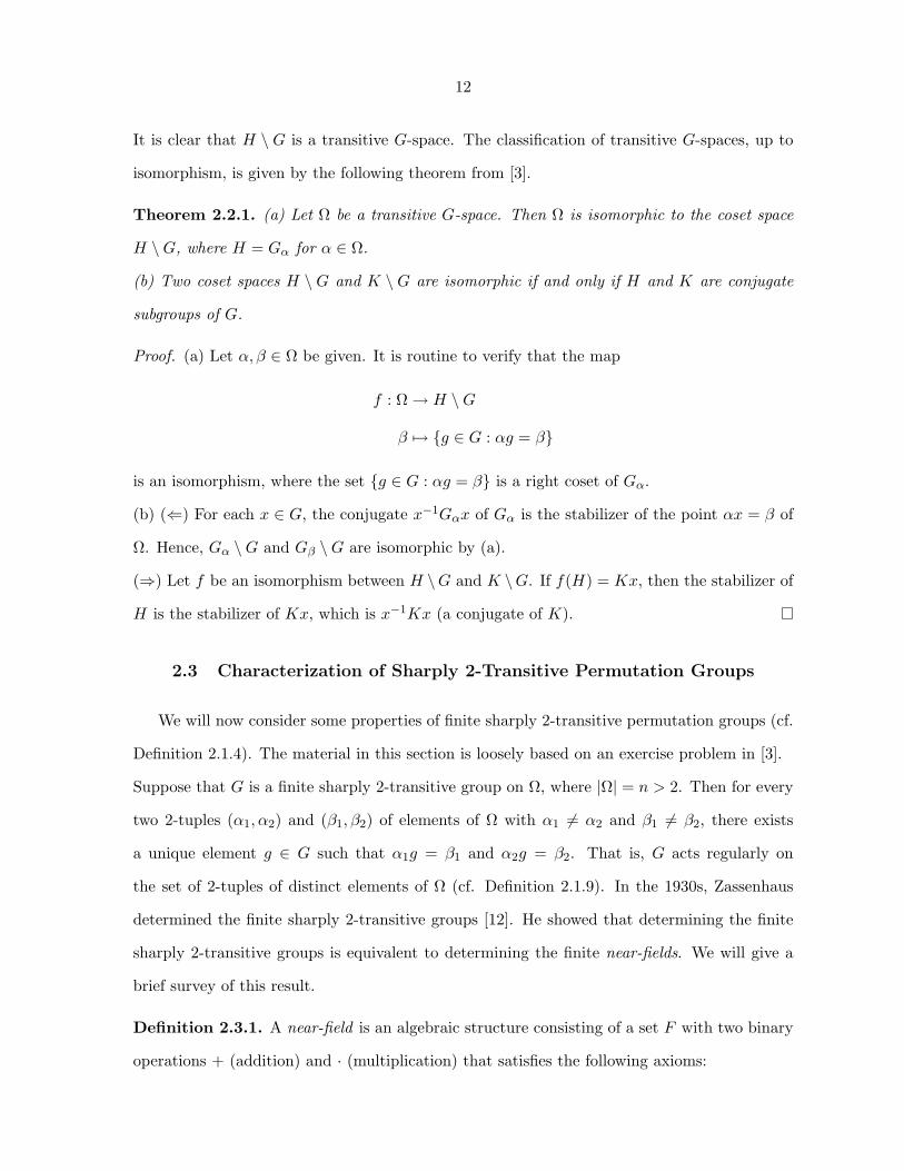
It is clear that H \ G is a transitive G-space. The classification of transitive G-spaces, up to

isomorphism, is given by the following theorem from [3].

Theorem 2.2.1. (a) Let Ω be a transitive G-space. Then Ω is isomorphic to the coset space

H \G, where H = Gα for α ∈ Ω.

(b) Two coset spaces H \ G and K \ G are isomorphic if and only if H and K are conjugate

subgroups of G.

Proof. (a) Let α, β ∈ Ω be given. It is routine to verify that the map

f : Ω→ H \G

β 7→ g ∈ G : αg = β

is an isomorphism, where the set g ∈ G : αg = β is a right coset of Gα.

(b) (⇐) For each x ∈ G, the conjugate x−1Gαx of Gα is the stabilizer of the point αx = β of

Ω. Hence, Gα \G and Gβ \G are isomorphic by (a).

(⇒) Let f be an isomorphism between H \G and K \G. If f(H) = Kx, then the stabilizer of

H is the stabilizer of Kx, which is x−1Kx (a conjugate of K).

2.3 Characterization of Sharply 2-Transitive Permutation Groups

We will now consider some properties of finite sharply 2-transitive permutation groups (cf.

Definition 2.1.4). The material in this section is loosely based on an exercise problem in [3].

Suppose that G is a finite sharply 2-transitive group on Ω, where |Ω| = n > 2. Then for every

two 2-tuples (α1, α2) and (β1, β2) of elements of Ω with α1 6= α2 and β1 6= β2, there exists

a unique element g ∈ G such that α1g = β1 and α2g = β2. That is, G acts regularly on

the set of 2-tuples of distinct elements of Ω (cf. Definition 2.1.9). In the 1930s, Zassenhaus

determined the finite sharply 2-transitive groups [12]. He showed that determining the finite

sharply 2-transitive groups is equivalent to determining the finite near-fields. We will give a

brief survey of this result.

Definition 2.3.1. A near-field is an algebraic structure consisting of a set F with two binary

operations + (addition) and · (multiplication) that satisfies the following axioms:

13

(i) (F,+) is an abelian group.

(ii) For all x, y, z ∈ F , (x · y) · z = x · (y · z) (associative law for multiplication).

(iii) For all x, y, z ∈ F , (x+ y) · z = x · z + y · z (right distributive law).

(iv) There exists an element 1 ∈ F such that for all x ∈ F , 1 · x = x · 1 = x (multiplicative

identity).

(v) For each nonzero element x ∈ F , there exists x−1 ∈ F such that x · x−1 = 1 = x−1 · x

(multiplicative inverses).

Note that every field is a near-field. Zassenhaus classified the finite near-fields that are not

fields [3]. Most such near-fields are Dickson near-fields. They are obtained from fields by using

field automorphisms to “twist” the multiplication. There are also seven exceptional near-fields

with orders 52, 72, 112, 112, 232, 292, and 592, respectively.

Definition 2.3.2. Let F be a near-field with |F | = n, and let F ∗ = F \ 0. Define

A = τa,b : (a, b) ∈ F ∗ × F, and τa,b(x) = xa+ b for all x ∈ F.

We call A the group of affine transformations of the near-field F . Note that |A| = |F ∗| · |F | =

(n− 1)n.

Proposition 2.3.3. Given a near-field F , the group A of affine transformations is a sharply

2-transitive group on F .

Proof. It is routine to verify that A is a transitive permutation group on F . We claim that A

acts sharply 2-transitively on F . To see this, let (x1, y1), (x2, y2) ∈ F×F with x1 6= y1 and x2 6=

y2. Then the system of two equations τa,b(x1) = x1a+ b = x2 and τa,b(y1) = y1a+ b = y2 has

a unique solution a = (x1 − y1)−1(x2 − y2) and b = x2 − x1a = x2 − x1(x1 − y1)−1(x2 − y2).

That is, there exists a unique transformation τa,b = g ∈ A such that x1g = x2 and y1g = y2.

Therefore, A is a sharply 2-transitive group on F .

14

Example 2.3.4. Let F = Z5 = 0, 1, 2, 3, 4. So n = |F | = 5. Then

A = τ1,0, τ1,1, τ1,2, τ1,3, τ1,4,

τ2,0, τ2,1, τ2,2, τ2,3, τ2,4,

τ3,0, τ3,1, τ3,2, τ3,3, τ3,4,

τ4,0, τ4,1, τ4,2, τ4,3, τ4,4.

Note that τ1,0 = 1 (identity) since for all x ∈ F , τ1,0(x) = 1 · x + 0 = x. The transfor-

mations τ1,1, τ1,2, τ1,3, τ1,4 are the translates x 7→ x + 1, x 7→ x + 2, x 7→ x + 3, x 7→ x + 4,

respectively, and have no fixed points. The point stabilizers are A0 = τ1,0, τ2,0, τ3,0, τ4,0,

A1 = τ1,0, τ2,4, τ3,3, τ4,2, A2 = τ1,0, τ2,3, τ3,1, τ4,4, A3 = τ1,0, τ2,2, τ3,4, τ4,1, and A4 =

τ1,0, τ2,1, τ3,2, τ4,3. We note that each of the 15 elements in Ai\τ1,0 for i ∈ 0, 1, 2, 3, 4 fixes

exactly one point, while 4 translates τ1,1, τ1,2, τ1,3, τ1,4 fix no points and the unique element

1 = τ1,0 fixes all points of F = Z5. The set H consisting of the identity and the elements that

fix no points is a subgroup of A. The group table for H = τ1,0, τ1,1, τ1,2, τ1,3, τ1,4 is given

below.

τ1,0 τ1,1 τ1,2 τ1,3 τ1,4

τ1,0 τ1,0 τ1,1 τ1,2 τ1,3 τ1,4

τ1,1 τ1,1 τ1,2 τ1,3 τ1,4 τ1,0

τ1,2 τ1,2 τ1,3 τ1,4 τ1,0 τ1,1

τ1,3 τ1,3 τ1,4 τ1,0 τ1,1 τ1,2

τ1,4 τ1,4 τ1,0 τ1,1 τ1,2 τ1,3

We observe that τ1,α τ1,β = τ1,(α+β)(mod 5), for all α, β ∈ Z5. Therefore, the group (H, ) is

isomorphic to an additive group of order 5. The point stabilizer A1 = τ1,0, τ2,4, τ3,3, τ4,2 for

the element 1 ∈ F is also a subgroup of A. The group table for A1 is given below.

15

τ1,0 τ2,4 τ3,3 τ4,2

τ1,0 τ1,0 τ2,4 τ3,3 τ4,2

τ2,4 τ2,4 τ4,2 τ1,0 τ3,3

τ3,3 τ3,3 τ1,0 τ4,2 τ2,4

τ4,2 τ4,2 τ3,3 τ2,4 τ1,0

Proposition 2.3.5. Every finite sharply 2-transitive group G on Ω is realized as the affine

transformation group A of a near-field F such that G ∼= A and |Ω| = |F |.

Proof. First, we will show that every sharply 2-transitive group G has an abelian regular

normal subgroup. We observe that G contains no element except the identity that fixes more

than one point of Ω = ø1, ø2, · · · , øn. To see this, suppose that an element g ∈ G fixes

two distinct points øi, øj ∈ Ω. Then øig = øi and øjg = øj . Therefore, (øi, øj)g = (øi, øj).

By sharp 2-transitivity, it follows that g = 1, the identity of G. Next, we will prove that G

contains n(n− 2) elements that fix exactly one point. Given two 2-tuples (ø1, ø2) and (ø1, øi)

with i ∈ 3, 4, · · · , n, there exists a unique element gi ∈ G such that (ø1, ø2)gi = (ø1, øi).

The group elements gi, gj must be different for i, j ∈ 3, 4, · · · , n whenever i 6= j. So the

stabilizer Gø1 of ø1 contains exactly n − 2 non-identity elements. Clearly, this number is

the same for all øi ∈ Ω. We have that Gøi ∩ Gøj = 1 whenever i 6= j. Since the sets

Gø1 \ 1, Gø2 \ 1, · · · , Gøn \ 1 are disjoint, there exist exactly n(n− 2) elements of G that

fix exactly one point. By the above remark, the length of each orbit øGi is n. That is, |øGi | = n,

for all i ∈ 1, 2, · · · , n. By the orbit-stabilizer formula, |G| = |Gøi | · |øGi | = (n−1) ·n. That is,

|G| = n(n− 1). Only the identity fixes more than one point. We have that n(n− 2) elements

fix exactly one point, and one element (the identity) fixes all points. Therefore,

Number of elements with no fixed point = n(n− 1)− n(n− 2)− 1 = n− 1.

So there exist n−1 elements of G that fix no point. Now let A denote the set consisting of the

n− 1 fixed-point-free elements and the identity of G. Note that |A| = (n− 1) + 1 = n = |Ω|.

We will prove that the set A is a regular normal subgroup of G. Note that for all x, y ∈ A,

the element xy is fixed-point-free. Therefore, A is a subgroup of G. To see that A is a regular

16

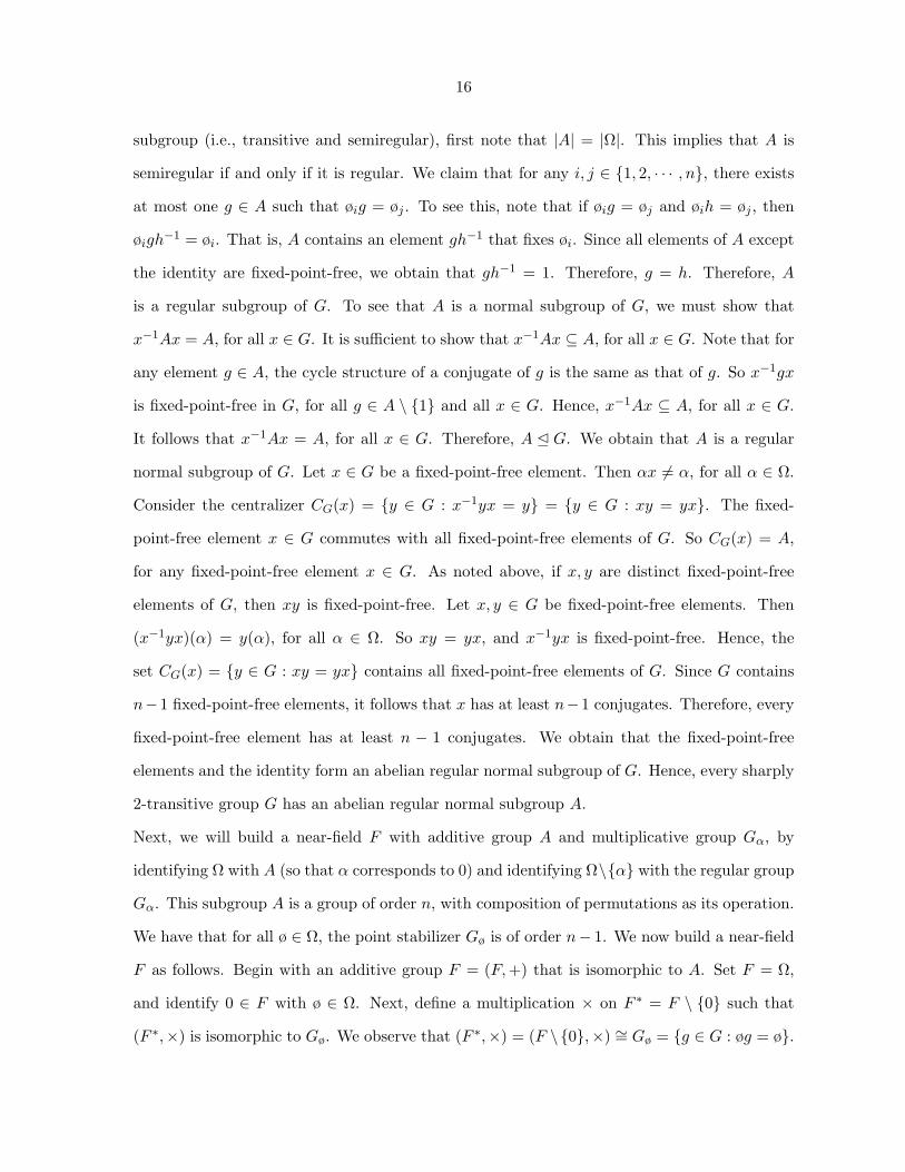
subgroup (i.e., transitive and semiregular), first note that |A| = |Ω|. This implies that A is

semiregular if and only if it is regular. We claim that for any i, j ∈ 1, 2, · · · , n, there exists

at most one g ∈ A such that øig = øj . To see this, note that if øig = øj and øih = øj , then

øigh−1 = øi. That is, A contains an element gh−1 that fixes øi. Since all elements of A except

the identity are fixed-point-free, we obtain that gh−1 = 1. Therefore, g = h. Therefore, A

is a regular subgroup of G. To see that A is a normal subgroup of G, we must show that

x−1Ax = A, for all x ∈ G. It is sufficient to show that x−1Ax ⊆ A, for all x ∈ G. Note that for

any element g ∈ A, the cycle structure of a conjugate of g is the same as that of g. So x−1gx

is fixed-point-free in G, for all g ∈ A \ 1 and all x ∈ G. Hence, x−1Ax ⊆ A, for all x ∈ G.

It follows that x−1Ax = A, for all x ∈ G. Therefore, A E G. We obtain that A is a regular

normal subgroup of G. Let x ∈ G be a fixed-point-free element. Then αx 6= α, for all α ∈ Ω.

Consider the centralizer CG(x) = y ∈ G : x−1yx = y = y ∈ G : xy = yx. The fixed-

point-free element x ∈ G commutes with all fixed-point-free elements of G. So CG(x) = A,

for any fixed-point-free element x ∈ G. As noted above, if x, y are distinct fixed-point-free

elements of G, then xy is fixed-point-free. Let x, y ∈ G be fixed-point-free elements. Then

(x−1yx)(α) = y(α), for all α ∈ Ω. So xy = yx, and x−1yx is fixed-point-free. Hence, the

set CG(x) = y ∈ G : xy = yx contains all fixed-point-free elements of G. Since G contains

n−1 fixed-point-free elements, it follows that x has at least n−1 conjugates. Therefore, every

fixed-point-free element has at least n − 1 conjugates. We obtain that the fixed-point-free

elements and the identity form an abelian regular normal subgroup of G. Hence, every sharply

2-transitive group G has an abelian regular normal subgroup A.

Next, we will build a near-field F with additive group A and multiplicative group Gα, by

identifying Ω with A (so that α corresponds to 0) and identifying Ω\α with the regular group

Gα. This subgroup A is a group of order n, with composition of permutations as its operation.

We have that for all ø ∈ Ω, the point stabilizer Gø is of order n− 1. We now build a near-field

F as follows. Begin with an additive group F = (F,+) that is isomorphic to A. Set F = Ω,

and identify 0 ∈ F with ø ∈ Ω. Next, define a multiplication × on F ∗ = F \ 0 such that

(F ∗,×) is isomorphic to Gø. We observe that (F ∗,×) = (F \0,×) ∼= Gø = g ∈ G : øg = ø.

17

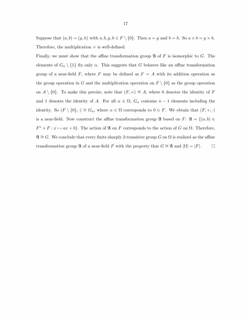
Suppose that (a, b) = (g, h) with a, b, g, h ∈ F \ 0. Then a = g and b = h. So a× b = g × h.

Therefore, the multiplication × is well-defined.

Finally, we must show that the affine transformation group A of F is isomorphic to G. The

elements of Gα \ 1 fix only α. This suggests that G behaves like an affine transformation

group of a near-field F , where F may be defined as F = A with its addition operation as

the group operation in G and the multiplication operation on F \ 0 as the group operation

on A \ 0. To make this precise, note that (F,+) ∼= A, where 0 denotes the identity of F

and 1 denotes the identity of A. For all α ∈ Ω, Gα contains n − 1 elements including the

identity. So (F \ 0, ·) ∼= Gα, where α ∈ Ω corresponds to 0 ∈ F . We obtain that (F,+, ·)

is a near-field. Now construct the affine transformation group A based on F : A = (a, b) ∈

F ∗ × F : x 7→ ax+ b. The action of A on F corresponds to the action of G on Ω. Therefore,

A ∼= G. We conclude that every finite sharply 2-transitive group G on Ω is realized as the affine

transformation group A of a near-field F with the property that G ∼= A and |Ω| = |F |.

18

CHAPTER 3. COHERENT CONFIGURATIONS

In this chapter, we will discuss some additional topics relevant to the study of permutation

groups.

3.1 Coherent Configurations and Basis Algebras

Next, we will discuss the concept of a coherent configuration and the associated basis

algebra. Let G be a permutation group acting on a set Ω. Consider the mapping from

G × (Ω × Ω) to Ω × Ω given by(g, (α, β)

)7→ (αg, βg), for all g ∈ G and all α, β ∈ Ω. The

orbits of this action are called 2-orbits (or orbitals) of G on Ω. We have that

(α, α)G = (αg, αg) : g ∈ G ⊆ (α, α) : α ∈ Ω.

Depending on G, the set (α, α)G may be a proper subset of (α, α) : α ∈ Ω. For i, j ∈

1, 2, · · · , n, define (αi, αj)G = (αig, αjg) : g ∈ G.

Case 1 (homogeneous case): If G acts on Ω transitively, then (αi, αi)G = (α, α) : α ∈ G for

all i ∈ 1, 2, · · · , n.

Case 2 (non-homogeneous case): If G acts non-transitively on Ω, then the diagonal relation is

partitioned into multiple 2-orbits.

Definition 3.1.1. Let R1, R2, · · · , Rt be the 2-orbits of G on Ω, with the following properties:

1. Ω × Ω = R1 ∪ R2 ∪ · · · ∪ Rt (disjoint union). That is, R1, R2, · · · , Rt is a partition of

Ω× Ω.

2. For all i ∈ 1, 2, · · · , t, there exists i′ ∈ 1, 2, · · · , t such that RTi = (β, α) : (α, β) ∈

Ri = Ri′ .

19

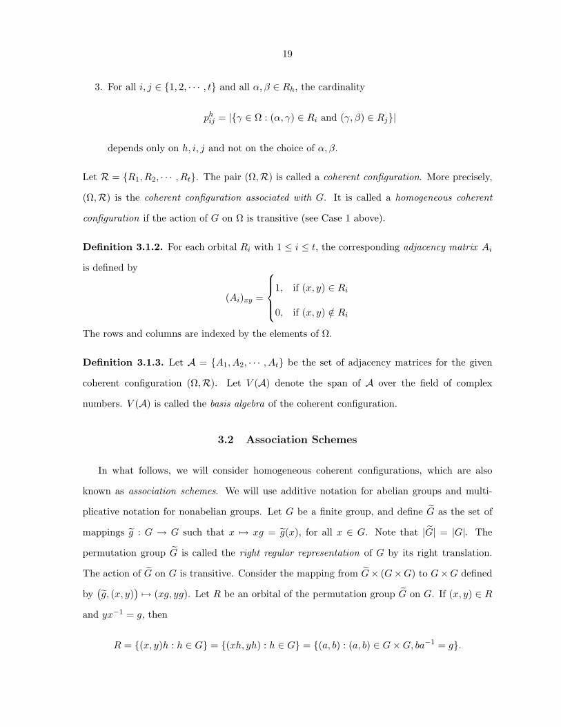
3. For all i, j ∈ 1, 2, · · · , t and all α, β ∈ Rh, the cardinality

phij = |γ ∈ Ω : (α, γ) ∈ Ri and (γ, β) ∈ Rj|

depends only on h, i, j and not on the choice of α, β.

Let R = R1, R2, · · · , Rt. The pair (Ω,R) is called a coherent configuration. More precisely,

(Ω,R) is the coherent configuration associated with G. It is called a homogeneous coherent

configuration if the action of G on Ω is transitive (see Case 1 above).

Definition 3.1.2. For each orbital Ri with 1 ≤ i ≤ t, the corresponding adjacency matrix Ai

is defined by

(Ai)xy =

1, if (x, y) ∈ Ri

0, if (x, y) /∈ Ri

The rows and columns are indexed by the elements of Ω.

Definition 3.1.3. Let A = A1, A2, · · · , At be the set of adjacency matrices for the given

coherent configuration (Ω,R). Let V (A) denote the span of A over the field of complex

numbers. V (A) is called the basis algebra of the coherent configuration.

3.2 Association Schemes

In what follows, we will consider homogeneous coherent configurations, which are also

known as association schemes. We will use additive notation for abelian groups and multi-

plicative notation for nonabelian groups. Let G be a finite group, and define G as the set of

mappings g : G → G such that x 7→ xg = g(x), for all x ∈ G. Note that |G| = |G|. The

permutation group G is called the right regular representation of G by its right translation.

The action of G on G is transitive. Consider the mapping from G× (G×G) to G×G defined

by(g, (x, y)

)7→ (xg, yg). Let R be an orbital of the permutation group G on G. If (x, y) ∈ R

and yx−1 = g, then

R = (x, y)h : h ∈ G = (xh, yh) : h ∈ G = (a, b) : (a, b) ∈ G×G, ba−1 = g.

20

Note that if (x, y)h = (xh, yh) = (a, b), then ba−1 = (yh)(h−1x−1) = yx−1 = g. Conversely,

suppose that (a, b) ∈ G×G with ba−1 = g. So b = ga. Let h = x−1a. Since a, x ∈ G, it follows

that h ∈ G. Then

(xh, yh) = (xx−1a, yx−1a) = (a, gxx−1a) = (a, ga) = (a, b).

Therefore, there exists h ∈ G such that (xh, yh) = (a, b). The orbital containing (x, y) where

yx−1 = g contains all pairs (a, b) with ba−1 = g. This means that there is a bijection between

the set of orbitals and G. Denote the orbital R = (a, b) : ba−1 = g by Rg. It is shown that

X(G) =(G, Rgg∈G

)is an association scheme. For a given group G, X(G) =

(G, Rgg∈G

)has the following properties, as discussed in [2].

1. The diagonal relation is given by R1 = (a, a) : a ∈ G ⊆ G×G, where 1 is the identity

of G. Also, ⋃g∈G

Rg = G×G

and Rg ∩Rh = ∅ whenever g 6= h. So the orbitals Rg form a partition of G×G.

2. For all g ∈ G, RTg = (y, x) : (x, y) ∈ Rg = Rg−1 . Note that if yx−1 = g, then

(yx−1)−1 = xy−1 = g−1, and so (y, x) ∈ Rg−1 . So the symmetric conjugate of every

relation in Rgg∈G also belongs to Rgg∈G.

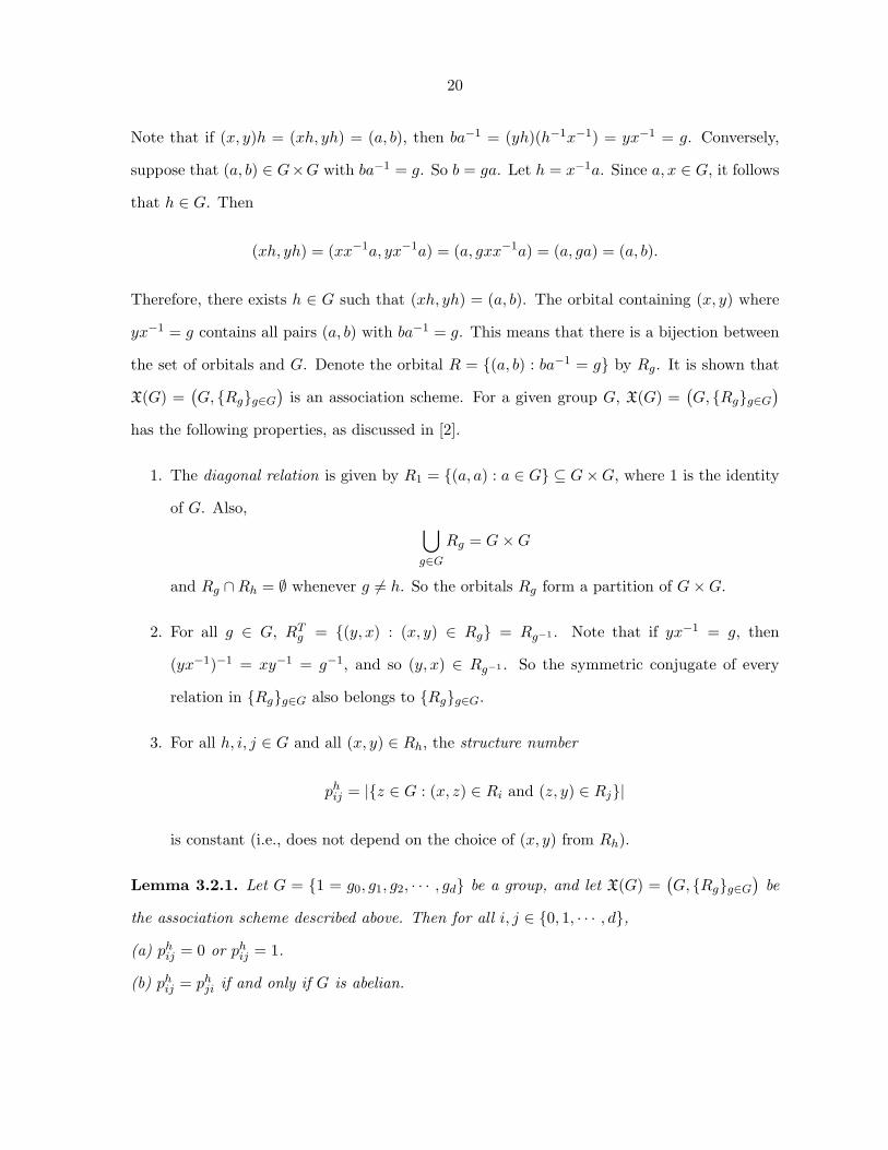
3. For all h, i, j ∈ G and all (x, y) ∈ Rh, the structure number

phij = |z ∈ G : (x, z) ∈ Ri and (z, y) ∈ Rj|

is constant (i.e., does not depend on the choice of (x, y) from Rh).

Lemma 3.2.1. Let G = 1 = g0, g1, g2, · · · , gd be a group, and let X(G) =(G, Rgg∈G

)be

the association scheme described above. Then for all i, j ∈ 0, 1, · · · , d,

(a) phij = 0 or phij = 1.

(b) phij = phji if and only if G is abelian.

21

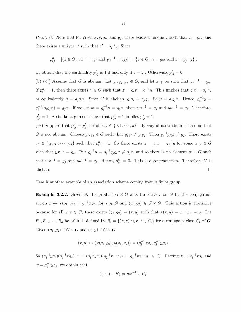
Proof. (a) Note that for given x, y, gi, and gj , there exists a unique z such that z = gix and

there exists a unique z′ such that z′ = g−1j y. Since

phij = |z ∈ G : zx−1 = gi and yz−1 = gj| = |z ∈ G : z = gix and z = g−1j y|,

we obtain that the cardinality phij is 1 if and only if z = z′. Otherwise, phij = 0.

(b) (⇐) Assume that G is abelian. Let gi, gj , gh ∈ G, and let x, y be such that yx−1 = gh.

If phij = 1, then there exists z ∈ G such that z = gix = g−1j y. This implies that gix = g−1

j y

or equivalently y = gjgix. Since G is abelian, gigj = gjgi. So y = gigjx. Hence, g−1i y =

g−1i (gigjx) = gjx. If we set w = g−1

i y = gjx, then wx−1 = gj and yw−1 = gi. Therefore,

phji = 1. A similar argument shows that phji = 1 implies phij = 1.

(⇒) Suppose that phij = phji for all i, j ∈ 0, 1, · · · , d. By way of contradiction, assume that

G is not abelian. Choose gi, gj ∈ G such that gjgi 6= gigj . Then g−1i gjgi 6= gj . There exists

gh ∈ g0, g1, · · · , gd such that phij = 1. So there exists z = gix = g−1j y for some x, y ∈ G

such that yx−1 = gh. But g−1i y = g−1

i gjgix 6= gjx, and so there is no element w ∈ G such

that wx−1 = gj and yw−1 = gi. Hence, phij = 0. This is a contradiction. Therefore, G is

abelian.

Here is another example of an association scheme coming from a finite group.

Example 3.2.2. Given G, the product G × G acts transitively on G by the conjugation

action x 7→ x(g1, g2) = g−11 xg2, for x ∈ G and (g1, g2) ∈ G × G. This action is transitive

because for all x, y ∈ G, there exists (g1, g2) = (x, y) such that x(x, y) = x−1xy = y. Let

R0, R1, · · · , Rd be orbitals defined by Ri = (x, y) : yx−1 ∈ Ci for a conjugacy class Ci of G.

Given (g1, g2) ∈ G×G and (x, y) ∈ G×G,

(x, y) 7→(x(g1, g2), y(g1, g2)

)= (g−1

1 xg2, g−11 yg2).

So (g−11 yg2)(g−1

1 xg2)−1 = (g−11 yg2)(g−1

2 x−1g1) = g−11 yx−1g1 ∈ Ci. Letting z = g−1

1 xg2 and

w = g−11 yg2, we obtain that

(z, w) ∈ Ri ⇔ wz−1 ∈ Ci.

22

Hence, we conclude that the association scheme obtained above by the action x 7→ g−11 xg2 for

all x ∈ G and all (g1, g2) ∈ G×G is isomorphic to the scheme defined by letting Ri = (x, y) :

yx−1 ∈ Ci, where e = C0, C1, C2, · · · , Cd are conjugacy classes of G.

We are now prepared to discuss some properties of association schemes. Let X =(X, Ri0≤i≤d

)be an association scheme of class d. We state the following axioms of an association scheme:

1. A0 +A1 + · · ·+Ad = J , the “all-ones” matrix.

2. For all i ∈ 0, 1, · · · , d, there exists i′ ∈ 0, 1, · · · , d such that ATi = Ai′ .

3. For all i, j ∈ 0, 1, · · · , d,

AiAj =d∑

h=0

phijAh = p0ijA0 + p1

ijA1 + · · ·+ pdijAd.

The span

〈A0, A1, · · · , Ad〉 = d∑i=0

aiAi : ai ∈ C

is a (d + 1)-dimensional subspace of M|X|(C). This subspace is closed under multiplication

and forms a ring.

Definition 3.2.3. The matrix algebra A = 〈I = A0, A1, A2, · · · , Ad〉 is called the Bose-Mesner

algebra of X.

3.3 Schur Rings

In this section, we will discuss a concept attributed to Issai Schur (1875-1941), whose work

in group theory and representation theory is chronicled in [4]. Some of the material in this

section is adapted from Chapter 4 of [10]. To see another presentation of X(G), consider the

group algebra C(G) =

∑g∈G

cgg : cg ∈ C

formed by the formal series

∑g∈G

cgg, cg ∈ C, with

formal basis element g ∈ G. The subring Z(G) =

∑g∈G

agg : ag ∈ Z

is called a group ring

over G. Later we will define the concept of a Schur ring, which is a particular subring of Z(G).

Definition 3.3.1. Let G be a group, and let e denote the identity element of G. In the group

ring Z(G), the element T =∑g∈T

g for any subset T ⊆ G is called a simple quantity.

23

Definition 3.3.2. A subring S of the group ring Z(G) is called a Schur ring (S-ring) over

G if S is a Z-module having a basis T0, T1, · · · , Td of simple quantities with the following

properties:

(S1) e = T0, T1, · · · , Td form a partition of G, and

(S2) For each i ∈ 0, 1, 2, · · · , d, T−1i = g−1 : g ∈ Ti = Ti′ for some i′ ∈ 0, 1, 2, · · · , d.

A set of simple quantities T0, T1, · · · , Td that gives rise to the Schur ring S = 〈T0, T1, · · · , Td〉

is called the standard basis for S. In this case, the integers phij such that

Ti · Tj =d∑

h=0

phijTh for i, j ∈ 0, 1, · · · , d

are called the structure numbers of S. Lemma 3.2.1 implies that for all i, j ∈ 0, 1, · · · , d,

Ti · Tj =d∑

h=0

phijTh =d∑

h=0

phjiTh = Tj · Ti.

That is, Ti · Tj = Tj · Ti for all i, j ∈ 0, 1, · · · , d. Here (g, h) ∈ Ri if and only if hg−1 ∈ Ti.

This implies that the scheme X(G) =(G, Ri0≤i≤d

)is commutative if and only if the group

G is abelian.

Note that in the examples below, (g, h) ∈ Ri ⇔ h− g ∈ Ti (since the groups are additive).

Example 3.3.3. Consider the cyclic group Z4 = 0, 1, 2, 3 and the group ring Z(Z4) =

a0 · 0 + a1 · 1 + a2 · 2 + a3 · 3 : ai ∈ Z = 〈0, 1, 2, 3〉. Define the Z-module S1 = 〈0, 1, 3, 2〉.

So T0 = 0, T1 = 1, 3, and T2 = 2. The following calculation in Z(Z4) (using simple

quantity notation) shows that S1 is an S-ring over Z4.

1, 3 · 1, 3 = 2 0 + 2 2

1, 3 · 2 = 1, 3

2 · 2 = 0.

The S-ring S1 is called the symmetrization of Z(Z4).

Example 3.3.4. Let G = Z6 = 0, 1, 2, 3, 4, 5. Consider the following three Z-modules:

S2,1 = 〈0, 1, 3, 2, 4, 5〉

S2,2 = 〈0, 2, 3, 4, 1, 5〉

S2 = 〈0, 1, 4, 2, 5, 3〉.

24

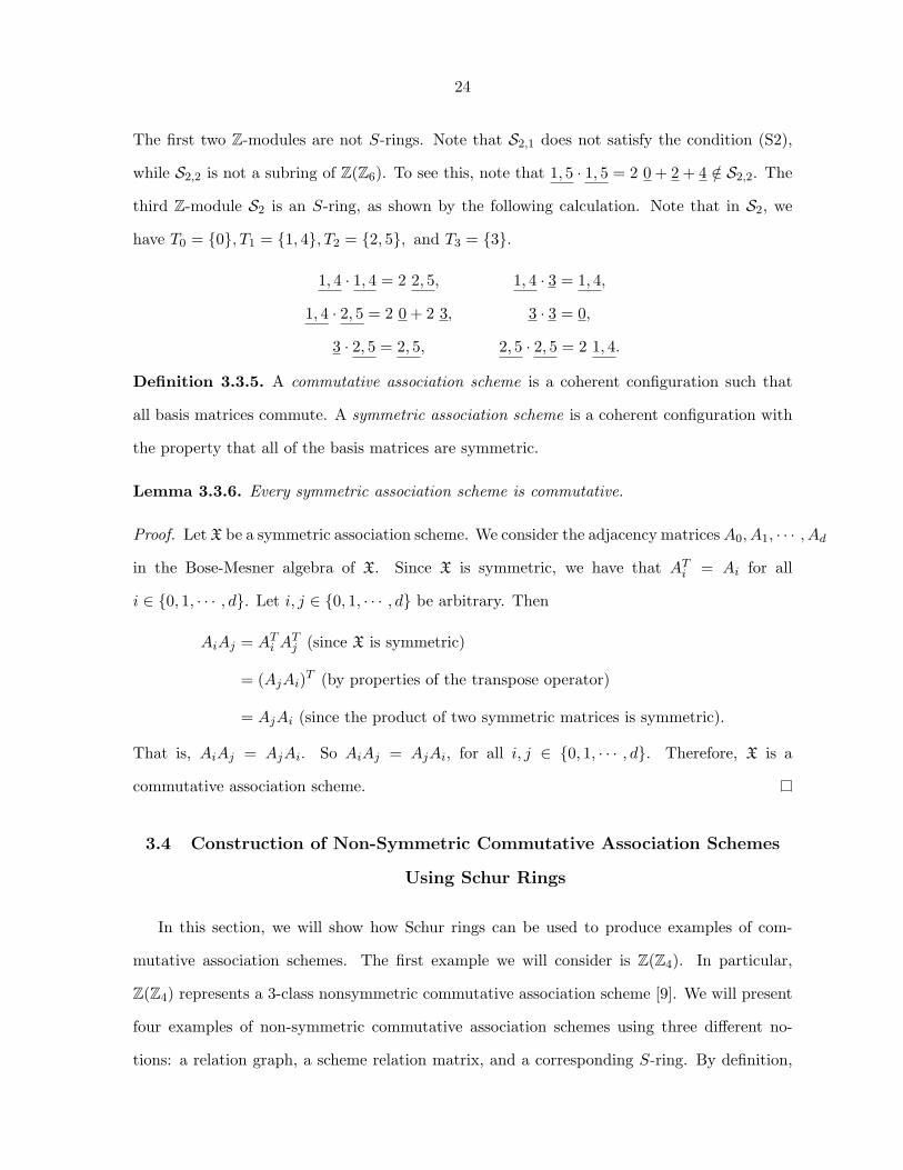
The first two Z-modules are not S-rings. Note that S2,1 does not satisfy the condition (S2),

while S2,2 is not a subring of Z(Z6). To see this, note that 1, 5 · 1, 5 = 2 0 + 2 + 4 /∈ S2,2. The

third Z-module S2 is an S-ring, as shown by the following calculation. Note that in S2, we

have T0 = 0, T1 = 1, 4, T2 = 2, 5, and T3 = 3.

1, 4 · 1, 4 = 2 2, 5, 1, 4 · 3 = 1, 4,

1, 4 · 2, 5 = 2 0 + 2 3, 3 · 3 = 0,

3 · 2, 5 = 2, 5, 2, 5 · 2, 5 = 2 1, 4.

Definition 3.3.5. A commutative association scheme is a coherent configuration such that

all basis matrices commute. A symmetric association scheme is a coherent configuration with

the property that all of the basis matrices are symmetric.

Lemma 3.3.6. Every symmetric association scheme is commutative.

Proof. Let X be a symmetric association scheme. We consider the adjacency matricesA0, A1, · · · , Ad

in the Bose-Mesner algebra of X. Since X is symmetric, we have that ATi = Ai for all

i ∈ 0, 1, · · · , d. Let i, j ∈ 0, 1, · · · , d be arbitrary. Then

AiAj = ATi ATj (since X is symmetric)

= (AjAi)T (by properties of the transpose operator)

= AjAi (since the product of two symmetric matrices is symmetric).

That is, AiAj = AjAi. So AiAj = AjAi, for all i, j ∈ 0, 1, · · · , d. Therefore, X is a

commutative association scheme.

3.4 Construction of Non-Symmetric Commutative Association Schemes

Using Schur Rings

In this section, we will show how Schur rings can be used to produce examples of com-

mutative association schemes. The first example we will consider is Z(Z4). In particular,

Z(Z4) represents a 3-class nonsymmetric commutative association scheme [9]. We will present

four examples of non-symmetric commutative association schemes using three different no-

tions: a relation graph, a scheme relation matrix, and a corresponding S-ring. By definition,

25

the scheme relation matrix A is given by Axy = i if and only if (x, y) ∈ Ri, for the scheme

X =(X, Ri0≤i≤d

). That is, A = A1+2A2+· · ·+dAd, where Ai denotes the adjacency matrix

of (X,Ri). The directed vertex-edge graphs corresponding to the scheme relation matrices are

also shown in the following examples.

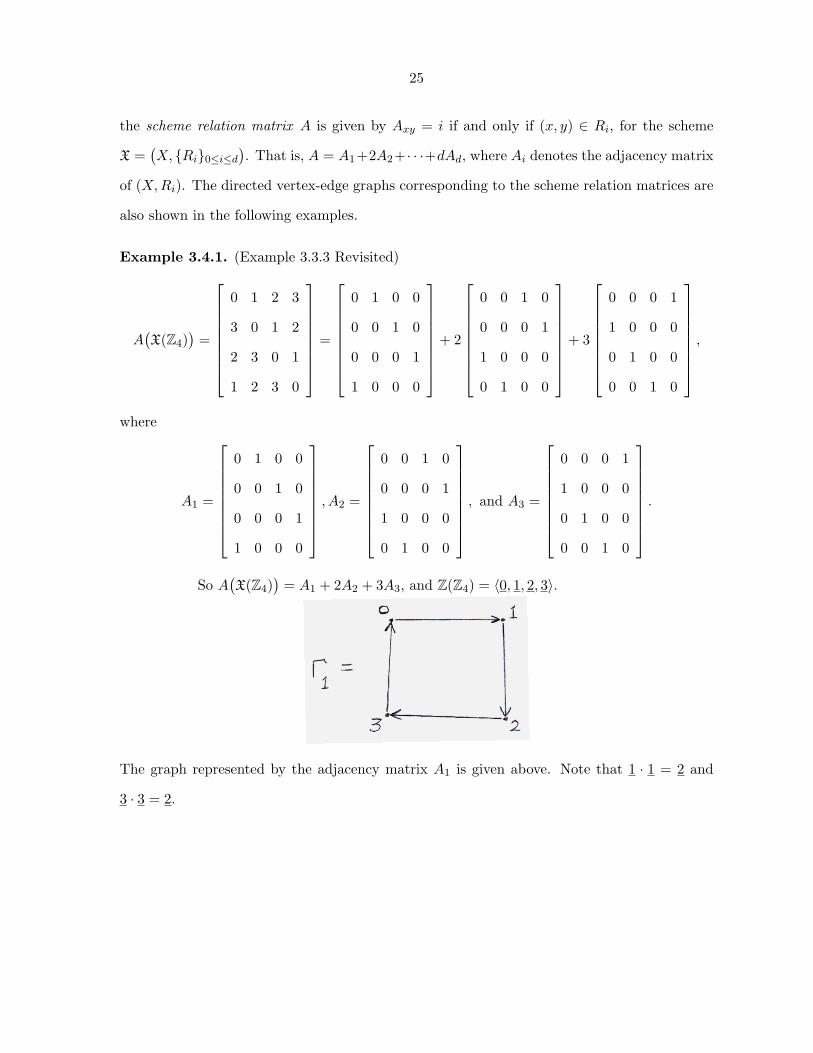
Example 3.4.1. (Example 3.3.3 Revisited)

A(X(Z4)

)=

0 1 2 3

3 0 1 2

2 3 0 1

1 2 3 0

=

0 1 0 0

0 0 1 0

0 0 0 1

1 0 0 0

+ 2

0 0 1 0

0 0 0 1

1 0 0 0

0 1 0 0

+ 3

0 0 0 1

1 0 0 0

0 1 0 0

0 0 1 0

,

where

A1 =

0 1 0 0

0 0 1 0

0 0 0 1

1 0 0 0

, A2 =

0 0 1 0

0 0 0 1

1 0 0 0

0 1 0 0

, and A3 =

0 0 0 1

1 0 0 0

0 1 0 0

0 0 1 0

.

So A(X(Z4)

)= A1 + 2A2 + 3A3, and Z(Z4) = 〈0, 1, 2, 3〉.

The graph represented by the adjacency matrix A1 is given above. Note that 1 · 1 = 2 and

3 · 3 = 2.

26

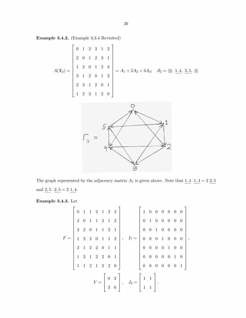
Example 3.4.2. (Example 3.3.4 Revisited)

A(X2) =

0 1 2 3 1 2

2 0 1 2 3 1

1 2 0 1 2 3

3 1 2 0 1 2

2 3 1 2 0 1

1 2 3 1 2 0

= A1 + 2A2 + 3A3; S2 = 〈0, 1, 4, 2, 5, 3〉

The graph represented by the adjacency matrix A1 is given above. Note that 1, 4 · 1, 4 = 2 2, 5

and 2, 5 · 2, 5 = 2 1, 4.

Example 3.4.3. Let

F =

0 1 1 2 1 2 2

2 0 1 1 2 1 2

2 2 0 1 1 2 1

1 2 2 0 1 1 2

2 1 2 2 0 1 1

1 2 1 2 2 0 1

1 1 2 1 2 2 0

, I7 =

1 0 0 0 0 0 0

0 1 0 0 0 0 0

0 0 1 0 0 0 0

0 0 0 1 0 0 0

0 0 0 0 1 0 0

0 0 0 0 0 1 0

0 0 0 0 0 0 1

,

Y =

0 3

3 0

, J2 =

1 1

1 1

.

27

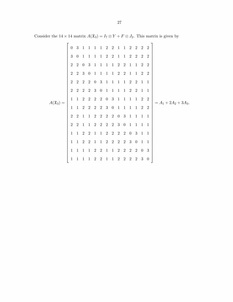
Consider the 14× 14 matrix A(X3) = I7 ⊗ Y + F ⊗ J2. This matrix is given by

A(X3) =

0 3 1 1 1 1 2 2 1 1 2 2 2 2

3 0 1 1 1 1 2 2 1 1 2 2 2 2

2 2 0 3 1 1 1 1 2 2 1 1 2 2

2 2 3 0 1 1 1 1 2 2 1 1 2 2

2 2 2 2 0 3 1 1 1 1 2 2 1 1

2 2 2 2 3 0 1 1 1 1 2 2 1 1

1 1 2 2 2 2 0 3 1 1 1 1 2 2

1 1 2 2 2 2 3 0 1 1 1 1 2 2

2 2 1 1 2 2 2 2 0 3 1 1 1 1

2 2 1 1 2 2 2 2 3 0 1 1 1 1

1 1 2 2 1 1 2 2 2 2 0 3 1 1

1 1 2 2 1 1 2 2 2 2 3 0 1 1

1 1 1 1 2 2 1 1 2 2 2 2 0 3

1 1 1 1 2 2 1 1 2 2 2 2 3 0

= A1 + 2A2 + 3A3.

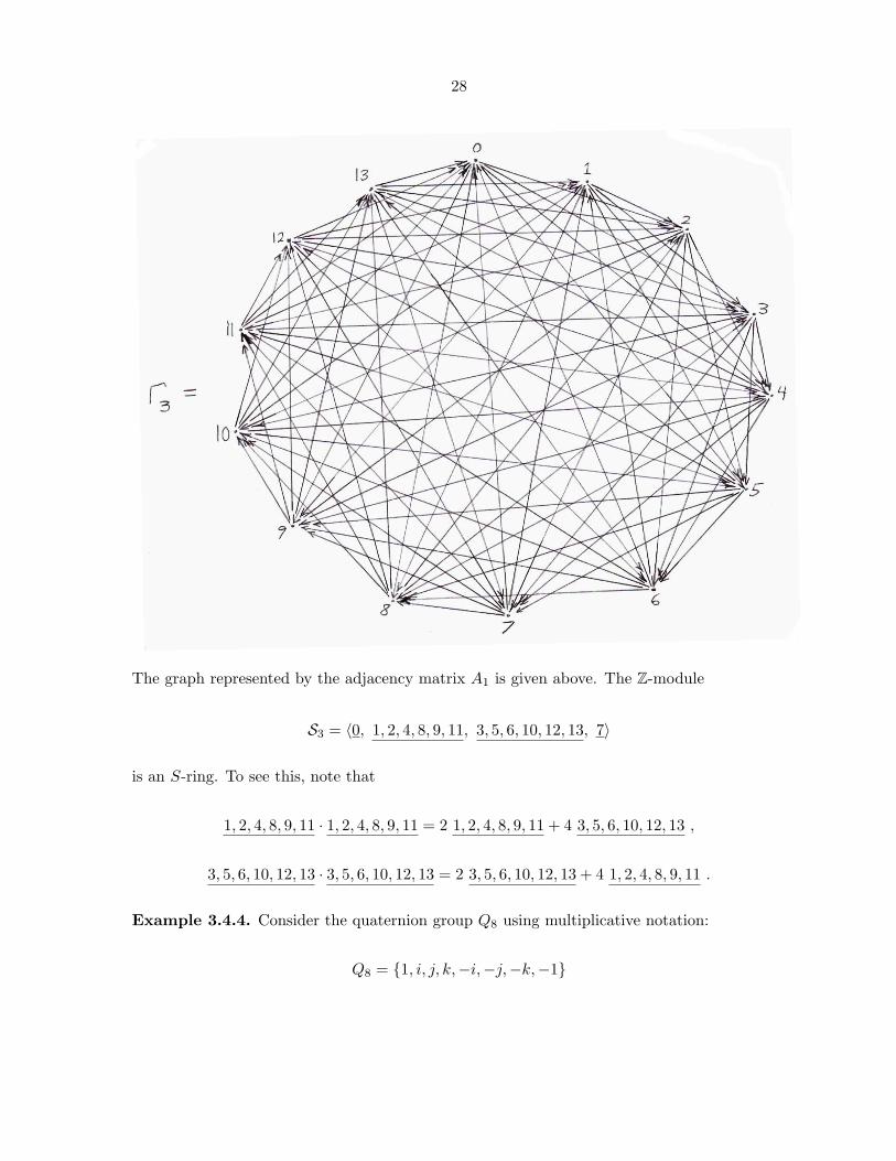
28

The graph represented by the adjacency matrix A1 is given above. The Z-module

S3 = 〈0, 1, 2, 4, 8, 9, 11, 3, 5, 6, 10, 12, 13, 7〉

is an S-ring. To see this, note that

1, 2, 4, 8, 9, 11 · 1, 2, 4, 8, 9, 11 = 2 1, 2, 4, 8, 9, 11 + 4 3, 5, 6, 10, 12, 13 ,

3, 5, 6, 10, 12, 13 · 3, 5, 6, 10, 12, 13 = 2 3, 5, 6, 10, 12, 13 + 4 1, 2, 4, 8, 9, 11 .

Example 3.4.4. Consider the quaternion group Q8 using multiplicative notation:

Q8 = 1, i, j, k,−i,−j,−k,−1

29

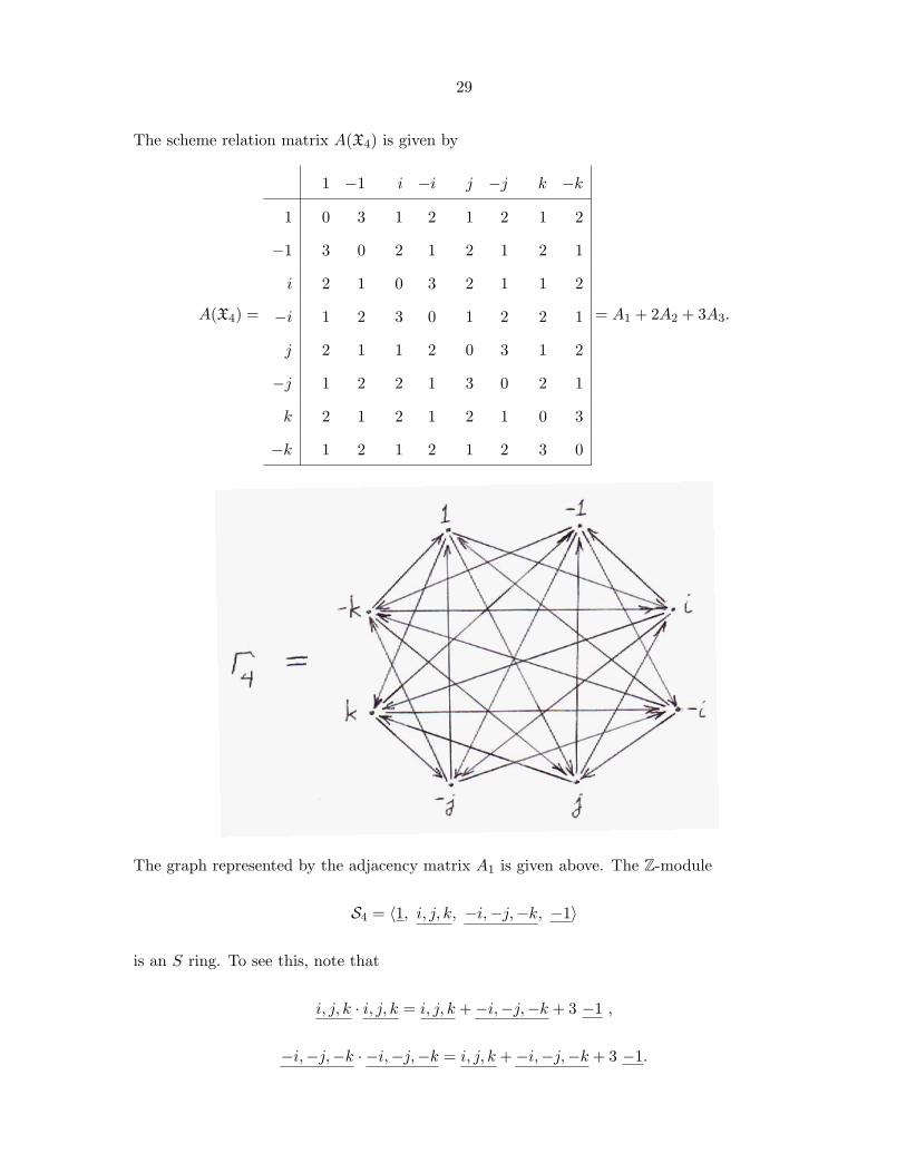
The scheme relation matrix A(X4) is given by

A(X4) =

1 −1 i −i j −j k −k

1 0 3 1 2 1 2 1 2

−1 3 0 2 1 2 1 2 1

i 2 1 0 3 2 1 1 2

−i 1 2 3 0 1 2 2 1

j 2 1 1 2 0 3 1 2

−j 1 2 2 1 3 0 2 1

k 2 1 2 1 2 1 0 3

−k 1 2 1 2 1 2 3 0

= A1 + 2A2 + 3A3.

The graph represented by the adjacency matrix A1 is given above. The Z-module

S4 = 〈1, i, j, k, −i,−j,−k, −1〉

is an S ring. To see this, note that

i, j, k · i, j, k = i, j, k +−i,−j,−k + 3 −1 ,

−i,−j,−k · −i,−j,−k = i, j, k +−i,−j,−k + 3 −1.

30

3.5 Permutation Representations and Centralizer Algebras

The relationship between groups and their representations is covered in many books in-

cluding [1]. We will now recall the important concepts of permutation representations and

centralizer algebras. Let G be a permutation group on Ω = ω1, ω2, · · · , ωn. Then each ele-

ment g ∈ G can be represented by a permutation matrix P (g), an n × n matrix of zeros and

ones, having (i, j)-entry

P (g)i,j =

1, if ωig = ωj

0, otherwise.

The map P : g 7→ P (g) is a group homomorphism from G to the general linear group GL(n,C),

the group of n× n nonsingular matrices over the field of complex numbers. The matrix P (g)

is called the permutation matrix corresponding to g.

The permutation g =

ω1 ω2 · · · ωn

ω1g ω2g · · · ωng

∈ SΩ induces the linear transformation

[ω1, ω2, · · · , ωn]P (g)T = [ω1g, ω2g, · · · , ωng].

The homomorphic image P (G) consisting of all matrices P (g) for g ∈ G is called the permu-

tation representation of G.

Definition 3.5.1. [2] The centralizer algebra of G is the set of n× n matrices that commute

with all of the permutation matrices P (g) for g ∈ G.

3.6 Character Theory

Suppose that G is a finite group. We define a matrix representation of G of degree n to be

a homomorphism M : G→ GL(n,C). So M(gh) = M(g)M(h), for all g, h ∈ G.

Definition 3.6.1. Let M,N be two matrix representations. We say that M and N are

equivalent if N(g) = X−1M(g)X for all g ∈ G, where X denotes an invertible matrix. In other

words, M and N are equivalent if they are related by a change of basis.

31

A representation M is said to be reducible if it is equivalent to a representation of the formM1(g) 0

∗ M2(g)

.We say that M is irreducible if it is not equivalent to such a representation. The matrix

representation M is decomposable if it is equivalent to a representationM1(g) 0

0 M2(g)

.If M is not equivalent to such a representation, we say that it is indecomposable.

Definition 3.6.2. The character of a representation M is the function χ : G→ C defined by

χ(g) = Trace M(g), for all g ∈ G.

The following theorem describes the relationship between matrix representations and charac-

ters.

Theorem 3.6.3. (a) Every character is constant on the conjugacy classes of G.

(b) Two matrix representations are equivalent if and only if they have the same character.

A character χ is said to be irreducible if it is the character of an irreducible representation [2].

The degree of a character χ is equal to the degree of the corresponding representation. We

can express any character as a sum of irreducible characters. The degree of any character χ is

equal to χ(1). The principal character of a group is the character of degree 1 that maps all

group elements to the number 1 ∈ C. For each element g ∈ G, the permutation character π is

given by

π(g) = ψ(g) (number of points fixed by g)

= number of ones on the diagonal of G

= trace of permutation matrix P (g).

Let Irr(G) denote the set of irreducible characters of G. We can decompose the permutation

character π into irreducible characters as follows:

π =∑

χ∈Irr(G)

mχ · χ.

32

The number mχ is called the multiplicity of χ. We say that π is multiplicity-free if every

constituent of π has multiplicity 1. That is, π is multiplicity-free if every irreducible character

appears at most once in the permutation character.

Definition 3.6.4. The Frobenius-Schur index of a character χ, denoted εχ, is the type of the

real irreducible representation that contains χ. It is given by

εχ =1|G|

∑g∈G

χ(g2).

Finally, we state the following theorem from [3].

Theorem 3.6.5. Suppose that G is a permutation group on Ω with permutation character π.

(a) The coherent configuration of G is a commutative association scheme if and only if π is

multiplicity-free.

(b) The coherent configuration of G is a symmetric association scheme if and only if π is

multiplicity-free and each of its irreducible constituents has Frobenius-Schur index +1.

33

BIBLIOGRAPHY

[1] J. L. Alperin and Rowen B. Bell (1995). Groups and Representations. Graduate Texts in

Mathematics 162. Springer-Verlag, 1995.

[2] E. Bannai and T. Ito (1984). Algebraic Combinatorics I. Benjamin/Cummings, 1984.

[3] P. J. Cameron (1999). Permutation Groups. London Mathematical Society Student Texts

45. Cambridge University Press, 1999.

[4] C. W. Curtis (1999). Pioneers of Representation Theory: Frobenius, Burnside, Schur, and

Brauer. History of Mathematics 15. American Mathematical Society, 1999.

[5] J. D. Dixon and B. Mortimer (1996). Permutation Groups. Graduate Texts in Mathematics

163. Springer-Verlag, 1996.

[6] D. S. Dummit and R. M. Foote (2004). Abstract Algebra. Third Edition. John Wiley and

Sons, 2004.

[7] G. Smith and O. Tabachnikova (2000). Topics in Group Theory. Springer-Verlag, 2000.

[8] V. P. Snaith (1998). Groups, Rings, and Galois Theory. World Scientific, 1998.

[9] S. Y. Song (1994). Class 3 association schemes whose symmetrizations have two classes,

J. Combin. Th. (A) 68 (1994).

[10] H. Wielandt (1964). Finite Permutation Groups. Academic Press, 1964.

[11] H. J. Zassenhaus (1958). The Theory of Groups. Chelsea Publishing Company, 1958.

[12] H. J. Zassenhaus (1936). Uber endliche Fastkorper, abh. Math. Sem. Hamburg 11 (1936),

187-220.

34

ACKNOWLEDGEMENTS

I wish to thank everyone who has helped me with my research. In particular, I would

like to thank my advisor, Dr. Sung-Yell Song. He is the best advisor in the world. Despite

his busy teaching schedule, he has spent many hours helping me to understand the important

concepts covered in this paper. He has also given me excellent guidance in writing the paper

and preparing for the final oral examination. I also want to thank Dr. Irvin Hentzel and Dr.

Jue Yan, my other two committee members. Dr. Hentzel’s encouragement and unique sense of

humor have helped me to persevere despite the challenges that I have encountered. Dr. Yan

has also offered many helpful suggestions and helped me to stay optimistic about my studies.

In addition, I thank Drs. Clifford Bergman, Elgin Johnston, Paul Sacks, Scott Hansen, and

Roger Maddux for everything that they have taught me in my mathematics courses here at

Iowa State University. I am also grateful for the encouragement of my mathematics professors

at Minnesota State University, Mankato, including Drs. Francis Hannick, Bruce Mericle, and

Namyong Lee. Finally, I thank my family for all of the support and encouragement that they

have provided throughout my years as a student of mathematics.