A Study about Kalman Filters Applied to Embedded Sensors

HAL Id: hal-01694026https://hal.archives-ouvertes.fr/hal-01694026

Submitted on 25 Jun 2019

HAL is a multi-disciplinary open accessarchive for the deposit and dissemination of sci-entific research documents, whether they are pub-lished or not. The documents may come fromteaching and research institutions in France orabroad, or from public or private research centers.

L’archive ouverte pluridisciplinaire HAL, estdestinée au dépôt et à la diffusion de documentsscientifiques de niveau recherche, publiés ou non,émanant des établissements d’enseignement et derecherche français ou étrangers, des laboratoirespublics ou privés.

A Study about Kalman Filters Applied to EmbeddedSensors

Aurelien Valade, Pascal Acco, Pierre Grabolosa, Jean-yves Fourniols

To cite this version:Aurelien Valade, Pascal Acco, Pierre Grabolosa, Jean-yves Fourniols. A Study about Kalman FiltersApplied to Embedded Sensors. Sensors, MDPI, 2017, 17 (12), pp.2810. �10.3390/s17122810�. �hal-01694026�

Article

A Study about Kalman Filters Applied toEmbedded Sensors

Aurélien Valade 1,2,*, Pascal Acco 1, Pierre Grabolosa 2 and Jean-Yves Fourniols 1

1 LAAS-CNRS, Université de Toulouse, CNRS, INSA, 31031 Toulouse, France; [email protected] (P.A.);[email protected] (J.-Y.F.)

2 Institut Méditerranéen d’Enseignement et de Recherche en Informatique et Robotique,66004 Perpignan, France; [email protected]

* Correspondence: [email protected]

Received: 27 October 2017; Accepted: 28 November 2017; Published: 5 December 2017

Abstract: Over the last decade, smart sensors have grown in complexity and can now handlemultiple measurement sources. This work establishes a methodology to achieve better estimates ofphysical values by processing raw measurements within a sensor using multi-physical models andKalman filters for data fusion. A driving constraint being production cost and power consumption,this methodology focuses on algorithmic complexity while meeting real-time constraints andimproving both precision and reliability despite low power processors limitations. Consequently,processing time available for other tasks is maximized. The known problem of estimating a 2Dorientation using an inertial measurement unit with automatic gyroscope bias compensation willbe used to illustrate the proposed methodology applied to a low power STM32L053 microcontroller.This application shows promising results with a processing time of 1.18 ms at 32 MHz with a 3.8%CPU usage due to the computation at a 26 Hz measurement and estimation rate.

Keywords: smart sensors; Kalman filters; algorithm complexity; IMU; compensation

1. Introduction

Since the “Smart Dust” project [1] from Berkeley in 1999, Smart Sensors technologies and theInternet of Things (IoT) have been growing fields of research, focussing on data collection andinterpretation [2]. The currently most used paradigm is to measure raw data from the sensor andsend the data to the cloud, or a computer, in order to be processed by complex algorithms [3,4].Another school behind those devices is to process sensor data within the sensor and provide the userwith a readily usable, filtered and normalized measurement. The resulting lower data throughput andlower latency allow for lower consumption in wireless applications and easier measurement usage.The ultimate goal would be compensating all sensor dispersion and deviation, independently ofenvironmental conditions, resulting in smart self correcting sensors.

The current and developing processing capabilities of sensors and the growing demand for SmartSensors, in a wide array of fields from hobbies to industrial automation, call for new embedded, in-line,real-time data processing applications. One of these applications is automatic and continuous sensorcalibration [5] with correction over time. Such a sensor does accelerate the manufacturing processesand provides more precise measurements over time, without costly human intervention or sensorreplacement due to age related deviation.

State of the art lab sensors, such as pH-meters or spectrometers, use systematic manualrecalibration procedures before each measurement to ensure good environmental conditions,dispersion, and deviation compensation. This method is, by definition, not applicable to embeddedsensors providing continuous and autonomous measurement without any external intervention.

Sensors 2017, 17, 2810; doi:10.3390/s17122810 www.mdpi.com/journal/sensors

Sensors 2017, 17, 2810 2 of 18

As most sensing elements are sensitive to multiple physical parameters, it is theoretically possibleto automatically enhance measurement precision by merging complementary sensors data usingmulti-physical parameters estimation. One such common method was initially presented by Kalman in1960 [6] and is known as the Kalman filter. This filter is a specialization of Bayesian filters [7] restrictedto discrete time, linear systems with Gaussian noise, and a state space model of the system. Such afilter allows estimating the internal state of a system based on its measurements and model.

For the last 50 years, Kalman filters and its extensions for non-linear systems, Extended KalmanFilter (EKF) and Unscented Kalman Filter (UKF) [8], have been wildly used in various applicationssuch as satellites, spacecrafts or planes to help automatic control of the systems. Due to its computingcomplexity, it has however not been wildly used in embedded systems until recent improvementsto microcontrollers technologies and processing power. Such applications includes smartphones ordrones for pose estimation.

This paper discusses a multi-sensor and multi-physical model coupled with a Kalman filter toachieve precise continuous estimation of a physical value without environmental bias while constrainedto low processing power of embedded systems. Additionally, an automatic system re-calibrationprocedure in known conditions is derived.

The remainder of this paper is organized as follows: Section 2 summarizes the technicalbackground used for this work; Section 3 exposes the proposed methodology; Section 4 applies themethodology to a 2D orientation estimation problem based on inertial measurement units; Section 5exposes and discusses the results obtained with the application; Section 6 references the used materialsand methods; and Section 7 describes the conclusions and the future of this work.

2. Technical Background

A multi-physical system model is a multiple input/multiple outputs (MIMO) system withphysical values for some of its inputs, calibration values for some of its parameters andmulti-parametric equations relying on these values for its measurement outputs. Such a systemcan be described using the state space representation using two equations: an evolution equation andan output/measurement equation.

2.1. Modeling the System

The state space representation [9] is a common MIMO system modeling toolkit. It relies onthree vectors and two equations to describe the relation between the system commands, its state,and its outputs:

• an input vector U, containing all the system known inputs;• a state vector X, containing the system internal state, which will evolve depending on the inputs;• an output vector Y, containing the system outputs/measurement;• an evolution Equation (1), describing the evolution of the internal state of the system, depending on

the previous state and the command input vector; and• a measurement Equation (2), describing the measurements at the output of the system depending

on its state and its command input.

Xk+1 = f (Xk, Uk) (1)

Yk = h(Xk, Uk) (2)

Linear Equations (1) and (2) can be written as matrix operations, as illustrated in Equations (3)and (4).

Xk+1 = [A] · Xk + [B] ·Uk (3)

Yk = [C] · Xk + [D] ·Uk (4)

From this point, the system model can be classified into three categories:

Sensors 2017, 17, 2810 3 of 18

• linear systems, using linear evolution (Equation (3)) and linear measurement functions(Equation (4));

• non-linear systems, using non-linear evolution (Equation (1)) and measurement functions(Equation (2)); and

• mixed systems using, for instance, a linear evolution function (Equation (3)) and a non-linearmeasurement function (Equation (2)) (or Equations (1) and (4)).

This representation can be applied to large systems composed of multiple subsystems,whether those are coupled, uncoupled, or unidirectionally coupled-respectively dependent,independent, or semi-dependent. Unless coupled, the larger system can be decomposed into thesum of its uncoupled subsystems, enabling major optimizations for computational complexity [10].

2.2. Kalman Filters

As exposed earlier, Kalman filters rely on the state representation of a system. They are specializedBayesian estimators for linear systems with discrete time and Gaussian noises. To do the estimation,the Kalman filter updates Equations (3) and (4) to Equations (5) and (6), where Vk and Wk are stateand measurement noise vectors.

Xk+1 = [A] · Xk + [B] ·Uk + Vk (5)

Yk = [C] · Xk + [D] ·Uk + Wk (6)

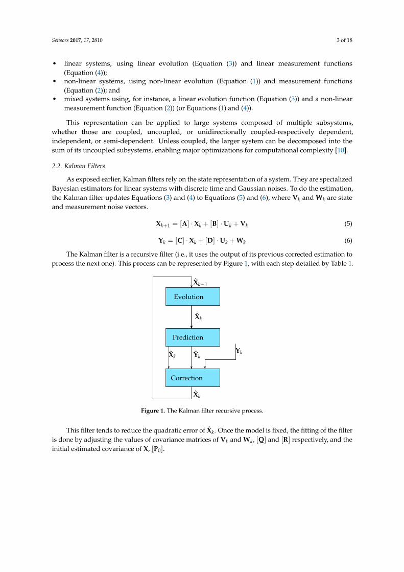
The Kalman filter is a recursive filter (i.e., it uses the output of its previous corrected estimation toprocess the next one). This process can be represented by Figure 1, with each step detailed by Table 1.

Evolution

Prediction

Correction

Xk

Xk YkYk

Xk

Xk−1

Figure 1. The Kalman filter recursive process.

This filter tends to reduce the quadratic error of Xk. Once the model is fixed, the fitting of the filteris done by adjusting the values of covariance matrices of Vk and Wk, [Q] and [R] respectively, and theinitial estimated covariance of X, [P0].

Sensors 2017, 17, 2810 4 of 18

Table 1. Kalman filter processing steps.

Step Kalman Filter Real System

Evolution Xk+1 = [A]Xk + [B]Uk Xk+1 = [A]Xk + [B]Uk + Vk[Pk+1] = [A][Pk][A]T + [Q]

Prediction/measurement Yk = [C]Xk + [D]Uk Yk = [C]Xk + [D]Uk + Wk

Correction

Ek = Yk − Yk[Kk] = [Pk][C]T([C][Pk][C]T + [R])−1

Xk = Xk + [Kk]Ek[Pk] = (I− [Kk][C])[Pk]

This filter has excellent estimation performances on well known linear system. For non-linearsystem, extensions have been developed, the best known being the Extended Kalman Filter (EKF) andthe Unscented Kalman Filter (UKF).

2.2.1. The Extended Kalman Filter

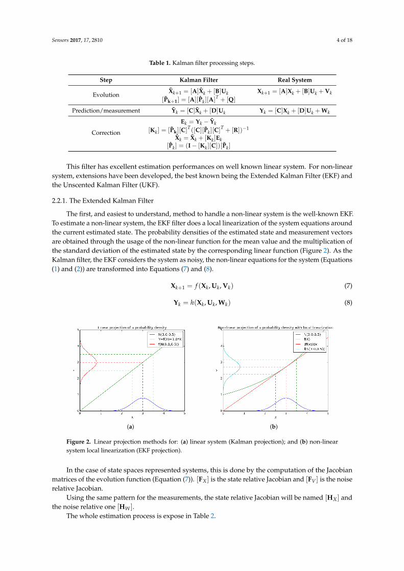
The first, and easiest to understand, method to handle a non-linear system is the well-known EKF.To estimate a non-linear system, the EKF filter does a local linearization of the system equations aroundthe current estimated state. The probability densities of the estimated state and measurement vectorsare obtained through the usage of the non-linear function for the mean value and the multiplication ofthe standard deviation of the estimated state by the corresponding linear function (Figure 2). As theKalman filter, the EKF considers the system as noisy, the non-linear equations for the system (Equations(1) and (2)) are transformed into Equations (7) and (8).

Xk+1 = f (Xk, Uk, Vk) (7)

Yk = h(Xk, Uk, Wk) (8)

(a) (b)

Figure 2. Linear projection methods for: (a) linear system (Kalman projection); and (b) non-linearsystem local linearization (EKF projection).

In the case of state spaces represented systems, this is done by the computation of the Jacobianmatrices of the evolution function (Equation (7)). [FX ] is the state relative Jacobian and [FV ] is the noiserelative Jacobian.

Using the same pattern for the measurements, the state relative Jacobian will be named [HX ] andthe noise relative one [HW ].

The whole estimation process is expose in Table 2.

Sensors 2017, 17, 2810 5 of 18

Table 2. EKF estimation steps.

Step EKF Real System

EvolutionXk+1 = f (Xk, Uk, 0) Xk+1 = f (Xk, Uk, Vk)

[Pk+1] = [FX,k+1][Pk][FX,k+1]T

+[FV,k+1][Q][FV,k+1]T

Prediction/measurement Yk = h(Xk, Uk, 0) Yk = h(Xk, Uk, Wk)

Correction

Ek = Yk − Yk[Kk] = [Pk][HX,k]

T([HX,k][Pk][HX,k]T + [R])−1

Xk = Xk + [Kk]Ek[Pk] = (I− [Kk][HX,k])[Pk]

This method’s main asset is its simplicity, as the operations are identical to the standard Kalmanfilter. The only addition is the computation of Jacobian matrices and the usage of non-linear functionsfor evolution and measurement predictions.

A known limitation is the slower convergence and instability of EKF compared to UKF whenapplied to systems with high non-linearities [11].

2.2.2. The Unscented Kalman Filter

To avoid large non-linearity estimation problems due to the local linearization used by the EKF,the UKF [12] was developed based on a mix between the Particle filter [13] and the Kalman filter.The method is based on the Unscented Transform to propagate the probability density directly throughthe non-linear function.

The Unscented Transform

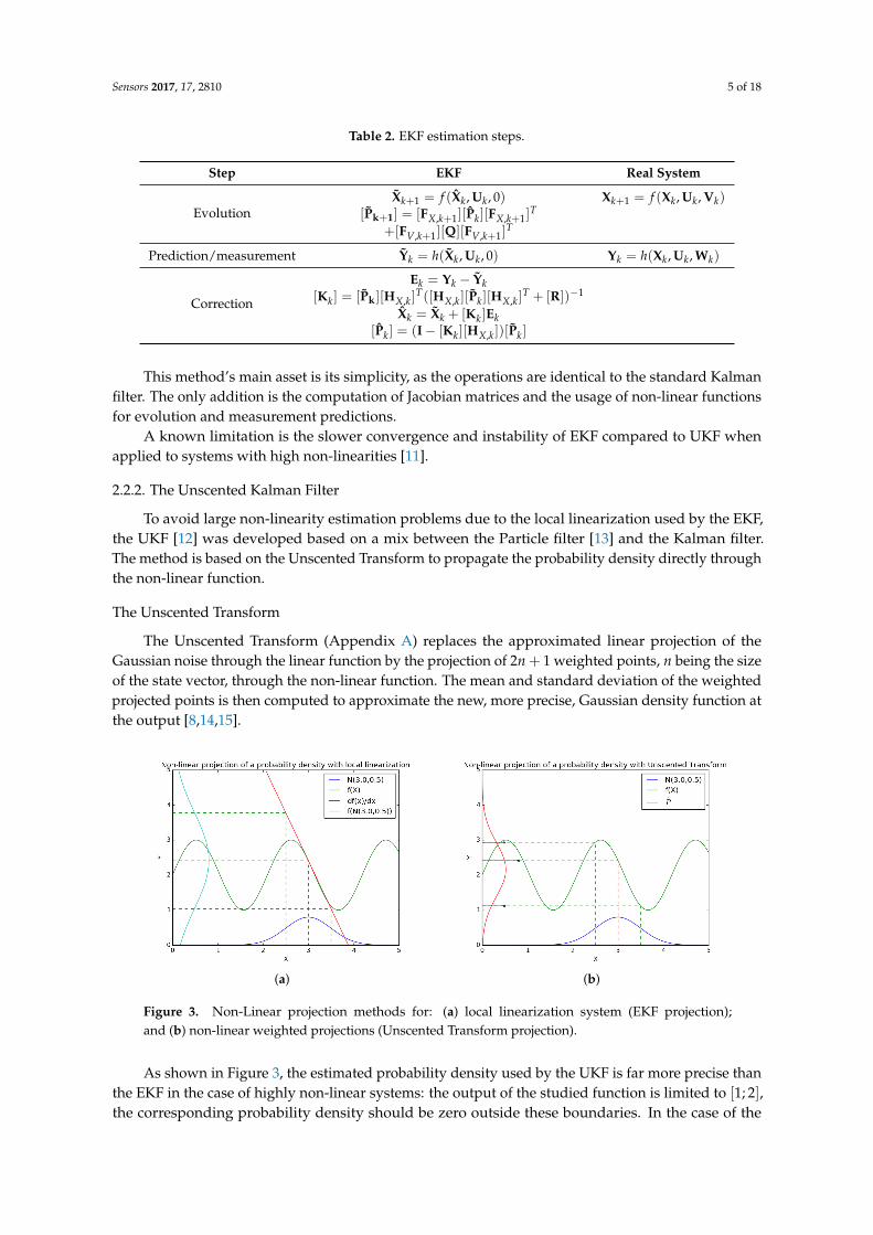
The Unscented Transform (Appendix A) replaces the approximated linear projection of theGaussian noise through the linear function by the projection of 2n + 1 weighted points, n being the sizeof the state vector, through the non-linear function. The mean and standard deviation of the weightedprojected points is then computed to approximate the new, more precise, Gaussian density function atthe output [8,14,15].

(a) (b)

Figure 3. Non-Linear projection methods for: (a) local linearization system (EKF projection);and (b) non-linear weighted projections (Unscented Transform projection).

As shown in Figure 3, the estimated probability density used by the UKF is far more precise thanthe EKF in the case of highly non-linear systems: the output of the studied function is limited to [1; 2],the corresponding probability density should be zero outside these boundaries. In the case of the

Sensors 2017, 17, 2810 6 of 18

local-linearization method with the selected input probability density, the probability of a value higherthan 2 is still important. On the other hand, with the Unscented Transform projection, the estimatedprobability density is far more coherent with the theoretical one.

Using this method, the computation for the UKF is decomposed into three steps: system evolution,measurements projection and correction.

System Evolution

• Generate a weighted point set for the following state estimation.

Xk =

[Xk, Xk +

√(n + λ)[Pk], Xk −

√(n + λ)[Pk]

](9)

With Xk a [n, 2n + 1] matrix representing the 2n + 1 states to propagate, weighted with ωc and ωµ

previously computed according to Appendix A. The spread of those states around the mean value isadjusted using the λ parameter. The square root of a matrix is defines as [B] =

√[A] ⇔ [B] · [B] =

[A], as explained in [16], and implies [A] is a square matrix.• Propagate the state through the evolution function

X (i)k+1 = f (X (i)

k , Uk, 0), i ∈ [0, 2n] (10)

• Compute the projection statistics using the Unscented method

Xk+1 =2n

∑i=0

ωµi X

(i)k+1 (11a)

[Pk+1] =2n

∑i=0

ωci (X

(i)k+1 − Xk+1)(X

(i)k+1 − Xk+1)

T + [Q] (11b)

Measurements Projection

• Generate a weighted point set from the estimated state

Xk+1 =

[Xk+1, Xk+1 +

√(n + λ)[Pk+1], Xk+1 −

√(n + λ)[Pk+1]

](12)

• Propagate the points through the measurement function

Y (i)k+1 = h(X (i)

k+1, Uk+1, 0), i ∈ [0, 2n] (13)

• Estimate the mean and covariance of the measurement

Yk+1 =2n

∑i=0

ωµi Y

(i)k+1 (14a)

[Pyy,k+1] =2n

∑i=0

ωci (Y

(i)k+1 − Yk+1)(Y

(i)k+1 − Yk+1)

T + [R] (14b)

• Estimate the crossed covariance between the state and measurement

[Pxy,k+1] =2n

∑i=0

ωci (X

(i)k+1 − Xk+1)(Y

(i)k+1 − Yk+1)

T (15)

Correction

• Compute the Kalman Gain[Kk+1] = [Pxy,k+1][Pyy,k+1]

−1 (16)

Sensors 2017, 17, 2810 7 of 18

• Correct the state

Xk+1 = Xk+1 + [Kk+1](Yk+1 − Yk+1) (17a)

[Pk+1] = [Pk+1]− [Kk+1][Pyy,k+1][Kk+1]T (17b)

With its precise projection, the UKF is much faster to converge and gives more precise resultson highly non-linear systems. This precision is possible at the expense of a far more computationalestimation process.

2.3. Algorithm Complexity and Computing Power

As the goal of this work is to provide a real-time estimation of the physical values on embeddedlow-power hardware, the processing time of the used algorithms has to be taken into account duringthe design. In this section, the algorithmic complexity of the different kinds of Kalman filters will bediscussed, and compared, taking into account the processing capabilities of common microcontrollers.

To compare the algorithm complexities, it is mandatory to choose a complexity indicator.The commonly used indicators are:

• the processed lines counts to do an operation;• the number of Multiplication and Accumulation (MAC) operations; and• the number of Floating point Operations (FLOP) ( i.e., the number of operation on “Real numbers”

in the algorithm).

In the case of operations on microcontrollers and matrix related operations, the FLOP is themost representative indicator for the algorithms complexity. Using this indicator, the mathematicaloperations relative to Kalman filtering will be discussed in the next part.

2.3.1. Algorithms Complexity

Kalman filtering is all about matrices and vectors operations, from the simple addition of twovectors to the inversion of a matrix. In those kinds of operations, algorithmic complexity can beexpressed in relation with the vectors and or matrices dimensions.

As an example, the steps required for the computation of the average of the components of avector of size n are:

• one affectation for the initialization of the sum variable;• one addition and affectation per element (n addictions and affectations);• one division; and• one affectation for the result.

Let’s define the following complexity indicators:

• T( f (n)), the number of operations to be executed to solve the problem; and• O( fO(n)) = limn→+∞ T( f (n)).

Then, the algorithmic complexity of the averaging operation is T(3 + 2n) with a complexity orderof O(2n). However, as the affectations can be considered as simple operations, the results can besimplified as T(1 + n), with an order of O(n).

Following the same method, we can get the complexities of every matrix operation as exposedin Table 3.

Sensors 2017, 17, 2810 8 of 18

Table 3. Matrix operations complexity sum-up.

Operation T(.) O(.)

Matrix multiplication 2× n×m× p 2× n×m× pAdding two vectors of size n n n

Adding two matrices of size (n, m) n×m n×mTranspose a matrix 0 0

Invert a matrix 4× n3 + 2× n2 4× n3

Mean vector of a matrix n× (m + 1) n×mMean value of a vector n + 1 n

Covariance de deux matrices 2× n×m× p 2× n×m× p

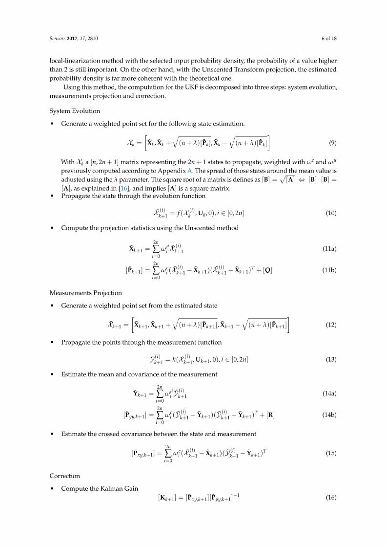
In the case of Kalman filters, the matrix inversions can be simplified by a factor of 2 as the matrix toinvert is Hermitian. The Cholesky inversion can be used in this case, giving a T(2n3 + n2) complexity,with an order of O(2n3) [17].

From this point, the Kalman filters complexity are shown in Table 4, using n as the state vectorsize, m as the measurement vector size and p as the command vector size.

Table 4. Kalman filtering complexity depending on n, m and p.

Algo Opération O(.)

(E)KF

Xk+1 = [A]Xk + [B]Uk 2n2

[Pk+1] = [A][Pk][A]T + [Q] 4n3

Yk = [C]Xk + [D]Uk 2m(n + p)Ek = Yk − Yk m

[Kk+1] = [Pk][C]T([C][Pk][C]T + [R])−1 4n2m/4m2nXk = Xk + [Kk]Ek 2mn

[Pk] = (I− [Kk][C])[Pk] ∼2n3/2m2n

UKF

Xk =

[Xk, Xk ±

√(n + λ)[Pk]

]n3

X (i)k+1 = f (X (i)

k ) 2nO( f (.))

Xk+1 = ∑2ni=0 ω

µi X

(i)k+1 4n2

[Pk+1] = ∑2ni=0 ωc

i (X(i)k+1 − Xk+1)(X

(i)k+1 − Xk+1)

T + [Q] 6n3

Y (i)k+1 = g(X (i)

k+1, Uk+1, 0) (2n + 1)O(g(.))

Yk+1 = ∑2ni=0 ω

µi Y

(i)k+1 4m2n

[Pyy,k+1] = ∑2ni=0 ωc

i (Y(i)k+1 − Yk+1)(Y

(i)k+1 − Yk+1)

T + [R] 6m2n

[Pxy,k+1] = ∑2ni=0 ωc

i (X(i)k+1 − Xk+1)(Y

(i)k+1 − Yk+1)

T 4n2mXk = Xk + [Kk]Ek 2mn

[Pk] = (I− [Kk][C])[Pk] ∼2n3/2m2n

As a result, the Kalman filters computing complexities are summed-up in the Table 5.

Table 5. Kalman filters complexity.

Algorithm T(.) O(.)

(E)KF 4n3 + 4m3 + 6m2n + 4n2m + 3n2 + · · · 4n3

UKF 10n3 + 4n2m + 14m2n + 23n2 + 6m2 + · · · 10n3

Using this analysis, the UKF algorithm demands about twice the computing time of an equivalentEKF algorithm, which can be decisive in small applications. Moreover, the computational complexityof these filters grows extremely fast with the size of the system model, limiting their real-time usage tobounded complexity system model, with reasonable state, command, and measurement vectors size.

Sensors 2017, 17, 2810 9 of 18

It also has to be noted that the previous study does not take into account the processing time of thenon-linear functions called by the EKF and UKF algorithms.

2.3.2. A Computing Power Overview

Embedded systems, and thus Smart Sensors, are mainly targeting low power consumption, sincemost of them are battery powered, and aim for low manufacturing costs. Consequently, such systemsare often designed around single core microcontroller architectures with low operating frequencies.Moreover, only high-end microcontrollers implement hardware Floating Point Unit (FPU) to acceleratethe computation of “real numbers”, due to their manufacturing cost and power consumption. Recenttechnological advances tend to improve this part [18].

Using this knowledge, the processing power of the used controller has to be acknowledged toensure the complexity of the filter is not too important to ensure real-time operations. As an example,the comparison can be done between three largely used microcontrollers:

• the ATMega328, a 8 bits microcontroller, the most commonly used in hobbyists designs as corecontroller of the Arduino Uno board;

• the STM32L053, a ultra low-consumption 32 bits microcontroller, used in the 2D orientationestimation demonstration; and

• the STM32F4xx, a high-end 32 bits microcontrollers family, embedding a FPU to acceleratecomputation of floating points numbers.

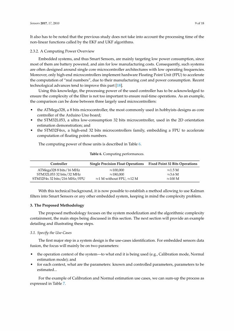
The computing power of those units is described in Table 6.

Table 6. Computing performances.

Controller Single Precision Float Operations Fixed Point 32 Bits Operations

ATMega328 8 bits/16 MHz ≈100,000 ≈1.5 MSTM32L053 32 bits/32 MHz ≈180,000 ≈3.6 M

STM32F4x 32 bits/216 MHz/FPU ≈1 M without FPU, ≈12 M ≈100 M

With this technical background, it is now possible to establish a method allowing to use Kalmanfilters into Smart Sensors or any other embedded system, keeping in mind the complexity problem.

3. The Proposed Methodology

The proposed methodology focuses on the system modelization and the algorithmic complexitycontainment, the main steps being discussed in this section. The next section will provide an exampledetailing and illustrating these steps.

3.1. Specify the Use-Cases

The first major step in a system design is the use-cases identification. For embedded sensors datafusion, the focus will mainly be on two parameters:

• the operation context of the system—to what end it is being used (e.g., Calibration mode, Normalestimation mode); and

• for each context, what are the parameters: known and controlled parameters, parameters to beestimated...

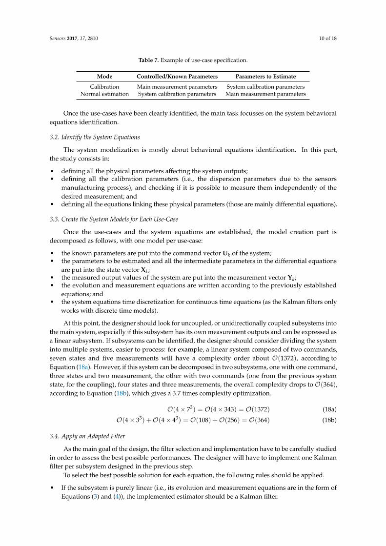
For the example of Calibration and Normal estimation use cases, we can sum-up the process asexpressed in Table 7.

Sensors 2017, 17, 2810 10 of 18

Table 7. Example of use-case specification.

Mode Controlled/Known Parameters Parameters to Estimate

Calibration Main measurement parameters System calibration parametersNormal estimation System calibration parameters Main measurement parameters

Once the use-cases have been clearly identified, the main task focusses on the system behavioralequations identification.

3.2. Identify the System Equations

The system modelization is mostly about behavioral equations identification. In this part,the study consists in:

• defining all the physical parameters affecting the system outputs;• defining all the calibration parameters (i.e., the dispersion parameters due to the sensors

manufacturing process), and checking if it is possible to measure them independently of thedesired measurement; and

• defining all the equations linking these physical parameters (those are mainly differential equations).

3.3. Create the System Models for Each Use-Case

Once the use-cases and the system equations are established, the model creation part isdecomposed as follows, with one model per use-case:

• the known parameters are put into the command vector Uk of the system;• the parameters to be estimated and all the intermediate parameters in the differential equations

are put into the state vector Xk;• the measured output values of the system are put into the measurement vector Yk;• the evolution and measurement equations are written according to the previously established

equations; and• the system equations time discretization for continuous time equations (as the Kalman filters only

works with discrete time models).

At this point, the designer should look for uncoupled, or unidirectionally coupled subsystems intothe main system, especially if this subsystem has its own measurement outputs and can be expressed asa linear subsystem. If subsystems can be identified, the designer should consider dividing the systeminto multiple systems, easier to process: for example, a linear system composed of two commands,seven states and five measurements will have a complexity order about O(1372), according toEquation (18a). However, if this system can be decomposed in two subsystems, one with one command,three states and two measurement, the other with two commands (one from the previous systemstate, for the coupling), four states and three measurements, the overall complexity drops to O(364),according to Equation (18b), which gives a 3.7 times complexity optimization.

O(4× 73) = O(4× 343) = O(1372) (18a)

O(4× 33) +O(4× 43) = O(108) +O(256) = O(364) (18b)

3.4. Apply an Adapted Filter

As the main goal of the design, the filter selection and implementation have to be carefully studiedin order to assess the best possible performances. The designer will have to implement one Kalmanfilter per subsystem designed in the previous step.

To select the best possible solution for each equation, the following rules should be applied.

• If the subsystem is purely linear (i.e., its evolution and measurement equations are in the form ofEquations (3) and (4)), the implemented estimator should be a Kalman filter.

Sensors 2017, 17, 2810 11 of 18

• If the subsystem is purely non-linear (i.e., its evolution and measurement equation are in the formof Equations (1) and (2)), the implemented estimator should be an EKF or UKF, depending on thenon-linearity, the state vector length and the available processing power.

• If the subsystem is mixed (i.e., its evolution equation is linear and its measurement equationis non-linear), the evolution part should be handled by Kalman filter implementation and themeasurement part should be implemented using EKF or UKF method, in order to optimize theprocessing load.

Finally, to optimize the processing time, some basic equations should be rewritten to their bareminimum: for example, a linear evolution equation in the form of Equation (19a) can be simplified to acouple of operations (Equations (19b) and (19c)) (Xk[n] being the nth element of the vector Xk).

Xk+1 =

[1 00 1

]· Xk +

[0 10 0

]·Uk (19a)

Xk+1[0] = Xk[0] + Uk[1] (19b)

Xk+1[1] = Xk[1] (19c)

In this example, the unoptimized version is composed of:

• two matrix multiplications by a vector, of complexity T(2× 2× 2× 1) = T(8) each; and• an addition of two vectors of two elements, of a complexity of T(2)

The optimized version is composed of one addition of two elements and two affectations (withvirtually no computational cost), which gives a complexity optimization of T(10) to T(1).

4. Application to a 2D Orientation Estimation Problem

The 2D orientation estimation is a common problem in robotics [19]. For instance, in a self-balancingrobot, the orientation of the robot has to be accurately measured at high speed in order to control thesystem using a feedback loop.

4.1. The Sensing Elements

To estimate the orientation of the robot in the XZ plane (Figure 4), the chosen approach relies ona three-axis accelerometer and three-axis gyroscope integrated circuit, the LSM6DSL sensor from STMicroelectronics. This circuit is used as a part of the development sensor board X-NUCLEO-IKS01A2 [20],which can be directly plugged on the microcontroller development board.

This sensor has the following features:

• raw measurements for the Accelerations and Rotational speed on X, Y and Z axis;• internal processing for free-fall detection, movement detection, 6D/4D orientation, click and

double-click detection, pedometer, step detector and counter;• an independent automatic sampling with data storage in FIFO;• I2C or SPI serial interface; and• two configurable interrupt output lines.

A corresponding driver library is also provided with the development kit for STM32development boards.

Sensors 2017, 17, 2810 12 of 18

Figure 4. Self-balancing robot orientation frame.

As for all sensors, the measurements on the accelerometer and gyroscope can be biased. In thefollowing study, only the gyroscope bias will be considered to have a significant impact on themeasurement and thus will be compensated.

4.2. The Processing Unit

As a processing unit, the ultra-low power STM32L053R8 has been selected, using thecorresponding Nucleo development kit. This microcontroller features:

• a low-power 32 MHz, 32 bits ARM Cortex-M0 processor, without FPU;• 64 KB of Flash and 8 KB of RAM;• a processing power of about 180 kFLOPs/s at 32 MHz; and• ultra low power consumption, with 88 µA/MHz running power consumption, and down to

270 nA Stand-by mode.

This microcontroller targets battery powered application, which is the main scope of thecurrent study.

4.3. Applying the Methodology

The first step to design the sensor requires in the use-cases listing establishment. The proposedsolution has two use-cases.

• Calibration mode: The sensor is still, on a table. Using this measurement, the gyroscopemeasurements should be zero, and the sensor bias is estimated by the filter.

• Orientation estimation mode: The sensor bias is known and used as a control input, and the sensororientation is estimated by the filter.

With the use-cases established, the system equations have to be written.

4.3.1. System Equations

To measure the 2D orientation of the system, the process relies on the measurement of the gravityacceleration by the accelerometers. This information is, however, sensitive to noise and parasiteaccelerations (e.g., chaos relative to the movement of the robot). The measurement stability is enhancedby the inclusion of gyroscope measurement, which assess the rotational speed.

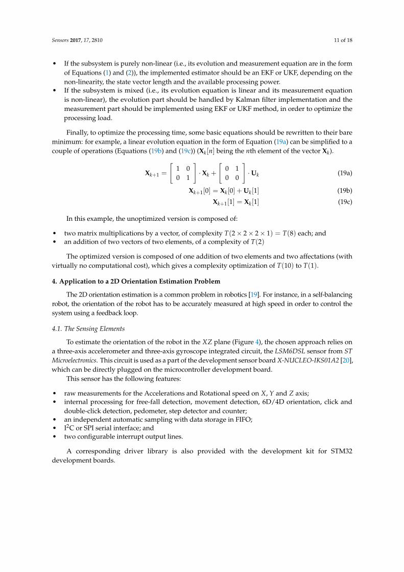
The equations express the projection of the gravity vector in the XZ 2D plane of the robot and themeasurement of its angle and norm (Figure 5).

Sensors 2017, 17, 2810 13 of 18

Figure 5. Gravity vector projection into the XZ plane.

Given this hypothesis, the three main parameters to the system are:

• the gravity vector projection norm |gravXZ|;• the gravity vector projection angle θY, which is the desired measurement translating the system

orientation in the 2D plane; and• the gyroscope measurement bias bgyro.

The system noises are:

• the acceleration noise on X and Z axes: Rax and Raz.

From these parameters, the sensor measurements are expressed as Equation (20a) for thegyroscope and Equations (20b) and (20c) for the accelerometers.

gY =δθY(t)

δt+ bgyro (20a)

ax = |gravXZ| ∗ sin(θY) + Rax (20b)

az = |gravXZ| ∗ cos(θY) + Raz (20c)

The system evolution can also be expressed by Equations (21a) and (21b).

δθY(t)δt

= gY − bgyro (21a)

δ|gravXZ|(t)δt

= 0 (21b)

At this point, the system equations have to be established for each use-case.

Calibration Mode Equations

In calibration mode, the system known input is the rotational velocity: the system being still,Equation (22) is valid.

δθY(t)δt

= 0 = gY − bgyro (22)

As the global system orientation is not relevant at this point, θ and |gXZ| will not be estimated inthis mode, and thus ax and az will not be monitored.

The state space equations for the calibration mode can be written as Equations (23a) and (23b).

Xcal,k+1 =(

bgyro,k+1

)= Xcal,k + Ucal,k =

(bgyro,k

)+ 0 (23a)

Ycal,k = (gY) = Xcal,k =(

bgyro,k

)(23b)

Sensors 2017, 17, 2810 14 of 18

When the system is stil, the gyroscope bias observation is trivial using this description.

Estimation Mode Equations

In estimation mode, the known input vector of the system is composed of the gyroscope bias.If the gyroscope noise is considered to be neglectable, the gyroscope Y axis measurement can also beadded to the command vector.

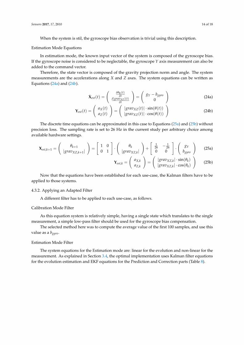
Therefore, the state vector is composed of the gravity projection norm and angle. The systemmeasurements are the accelerations along X and Z axes. The system equations can be written asEquations (24a) and (24b).

Xest(t) =

(δθY(t)

δtδ|gravXZ |(t)

δt

)=

(gY − bgyro

0

)(24a)

Yest(t) =

(aX(t)aZ(t)

)=

(|gravXZ(t)| · sin(θ(t))|gravXZ(t)| · cos(θ(t))

)(24b)

The discrete time equations can be approximated in this case to Equations (25a) and (25b) withoutprecision loss. The sampling rate is set to 26 Hz in the current study per arbitrary choice amongavailable hardware settings.

Xest,k+1 =

(θk+1

|gravXZ,k+1|

)=

[1 00 1

]·(

θk|gravXZ,k|

)+

[1

26 − 126

0 0

]·(

gYbgyro

)(25a)

Yest,k =

(aX,kaZ,k

)=

(|gravXZ,k| · sin(θk)

|gravXZ,k| · cos(θk)

)(25b)

Now that the equations have been established for each use-case, the Kalman filters have to beapplied to those systems.

4.3.2. Applying an Adapted Filter

A different filter has to be applied to each use-case, as follows.

Calibration Mode Filter

As this equation system is relatively simple, having a single state which translates to the singlemeasurement, a simple low-pass filter should be used for the gyroscope bias compensation.

The selected method here was to compute the average value of the first 100 samples, and use thisvalue as a bgyro.

Estimation Mode Filter

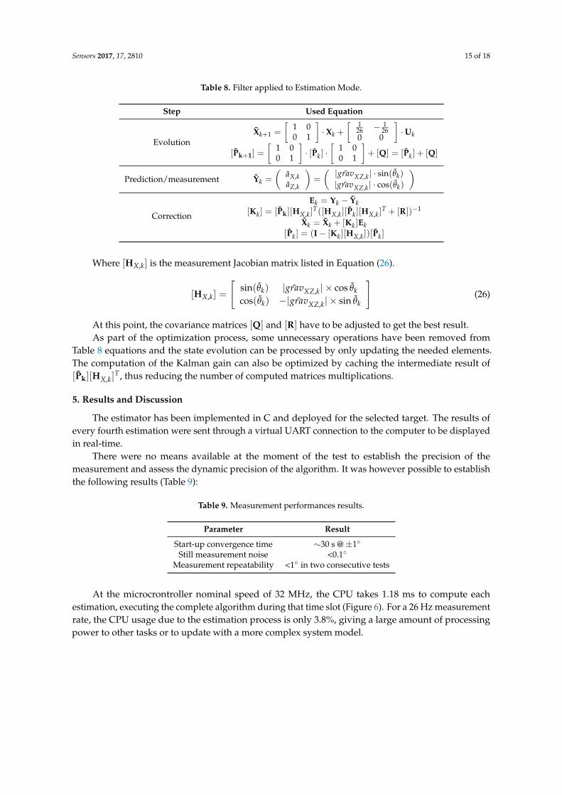
The system equations for the Estimation mode are: linear for the evolution and non-linear for themeasurement. As explained in Section 3.4, the optimal implementation uses Kalman filter equationsfor the evolution estimation and EKF equations for the Prediction and Correction parts (Table 8).

Sensors 2017, 17, 2810 15 of 18

Table 8. Filter applied to Estimation Mode.

Step Used Equation

EvolutionXk+1 =

[1 00 1

]· Xk +

[ 126 − 1

260 0

]·Uk

[Pk+1] =

[1 00 1

]· [Pk] ·

[1 00 1

]+ [Q] = [Pk] + [Q]

Prediction/measurement Yk =

(aX,kaZ,k

)=

(| ˜gravXZ,k| · sin(θk)

| ˜gravXZ,k| · cos(θk)

)

Correction

Ek = Yk − Yk[Kk] = [Pk][HX,k]

T([HX,k][Pk][HX,k]T + [R])−1

Xk = Xk + [Kk]Ek[Pk] = (I− [Kk][HX,k])[Pk]

Where [HX,k] is the measurement Jacobian matrix listed in Equation (26).

[HX,k] =

[sin(θk) | ˜gravXZ,k| × cos θkcos(θk) −| ˜gravXZ,k| × sin θk

](26)

At this point, the covariance matrices [Q] and [R] have to be adjusted to get the best result.As part of the optimization process, some unnecessary operations have been removed from

Table 8 equations and the state evolution can be processed by only updating the needed elements.The computation of the Kalman gain can also be optimized by caching the intermediate result of[Pk][HX,k]

T , thus reducing the number of computed matrices multiplications.

5. Results and Discussion

The estimator has been implemented in C and deployed for the selected target. The results ofevery fourth estimation were sent through a virtual UART connection to the computer to be displayedin real-time.

There were no means available at the moment of the test to establish the precision of themeasurement and assess the dynamic precision of the algorithm. It was however possible to establishthe following results (Table 9):

Table 9. Measurement performances results.

Parameter Result

Start-up convergence time ∼30 s @ ±1◦

Still measurement noise <0.1◦

Measurement repeatability <1◦ in two consecutive tests

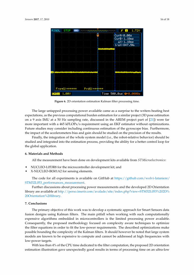
At the microcrontroller nominal speed of 32 MHz, the CPU takes 1.18 ms to compute eachestimation, executing the complete algorithm during that time slot (Figure 6). For a 26 Hz measurementrate, the CPU usage due to the estimation process is only 3.8%, giving a large amount of processingpower to other tasks or to update with a more complex system model.

Sensors 2017, 17, 2810 16 of 18

Figure 6. 2D orientation estimation Kalman filter processing time.

The large untapped processing power available came as a surprise to the writers beating bestexpectations, as the previous computational burden estimation for a similar project (3D pose estimationon a 9 axis IMU at a 50 Hz sampling rate, discussed in the AREM project part of [21]) were farmore important with a 465 kFLOPs/s requirement using an EKF estimator without optimizations.Future studies may consider including continuous estimation of the gyroscope bias. Furthermore,the impact of the accelerometers bias and gain should be studied on the precision of the results.

Finally, the integration of the whole system model (i.e., the robot-relative behavior) should bestudied and integrated into the estimation process, providing the ability for a better control loop forthe global application.

6. Materials and Methods

All the measurement have been done on development kits available from STMicroelectronics:

• NUCLEO-L053R8 for the microcontroller development kit; and• X-NUCLEO-IKS01A2 for sensing elements.

The code for all experiments is available on GitHub at https://github.com/wolvi-lataniere/STM32L053_performances_measurement.

Further discussions about processing power measurements and the developed 2D Orientationlibrary are available at http://perso.imerir.com/avalade/site/index.php?view=STM32L053%202D%20Orientation%20library.

7. Conclusions

The primary objective of this work was to develop a systematic approach for Smart Sensors datafusion designs using Kalman filters. The main pitfall when working with such computationallyexpensive algorithms embedded in microcontrollers is the limited processing power available.Consequently, the proposed methodology focused on complexity aware techniques to optimizethe filter equations in order to fit the low-power requirements. The described optimizations makepossible bounding the complexity of the Kalman filters. It should however be noted that large systemmodels are known to be expensive to compute and cannot be addressed at high frequencies withlow-power targets.

With less than 4% of the CPU time dedicated to the filter computation, the proposed 2D orientationestimation illustration gave unexpectedly good results in terms of processing time on an ultra-low

Sensors 2017, 17, 2810 17 of 18

power target. As a result, the writers attend to explore the capabilities of these optimized filters ona more complex application-specific model for the self-balancing robot in the near future.

The goal for the writers is to continue applying the methodology to a wider range of Smart Sensorsprojects, targeting new sensing elements, lower-end microcontrollers, and more complex models [21].

Acknowledgments: This research was done at Laboratoire d’Analyse et d’Architecture des Systèmes (LAAS-CNRS)and supported by TE Connectivity. This article redaction was supported by Institut Méditeranéen d’Enseignement etde Recherche en Informatique et Robotique (IMERIR).

Author Contributions: Aurélien Valade conceived this manuscript and wrote it, Pierre Grabolosa, Jean-Yves Fourniols,and Pascal Acco participated as technical and scientific advisors.

Conflicts of Interest: The authors declare no conflict of interest.

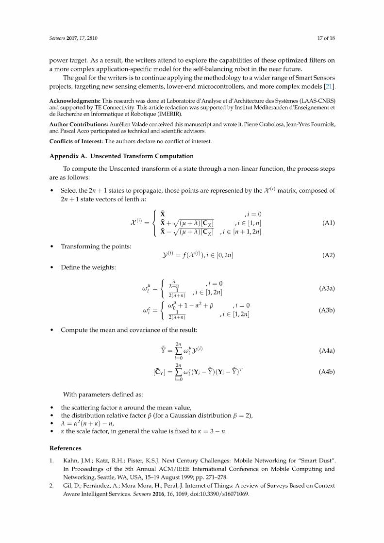
Appendix A. Unscented Transform Computation

To compute the Unscented transform of a state through a non-linear function, the process stepsare as follows:

• Select the 2n + 1 states to propagate, those points are represented by the X (i) matrix, composed of2n + 1 state vectors of lenth n:

X (i) =

X , i = 0X +

√(µ + λ)[CX ] , i ∈ [1, n]

X−√(µ + λ)[CX ] , i ∈ [n + 1, 2n]

(A1)

• Transforming the points:Y (i) = f (X (i)), i ∈ [0, 2n] (A2)

• Define the weights:

ωµi =

{λ

λ+n , i = 01

2(λ+n) , i ∈ [1, 2n] (A3a)

ωci =

{ω

µ0 + 1− α2 + β , i = 0

12(λ+n) , i ∈ [1, 2n] (A3b)

• Compute the mean and covariance of the result:

Y =2n

∑i=0

ωµi Y

(i) (A4a)

[CY] =2n

∑i=0

ωci (Yi − Y)(Yi − Y)T (A4b)

With parameters defined as:

• the scattering factor α around the mean value,• the distribution relative factor β (for a Gaussian distribution β = 2),• λ = α2(n + κ)− n,• κ the scale factor, in general the value is fixed to κ = 3− n.

References

1. Kahn, J.M.; Katz, R.H.; Pister, K.S.J. Next Century Challenges: Mobile Networking for “Smart Dust”.In Proceedings of the 5th Annual ACM/IEEE International Conference on Mobile Computing andNetworking, Seattle, WA, USA, 15–19 August 1999; pp. 271–278.

2. Gil, D.; Ferrández, A.; Mora-Mora, H.; Peral, J. Internet of Things: A review of Surveys Based on ContextAware Intelligent Services. Sensors 2016, 16, 1069, doi:10.3390/s16071069.

Sensors 2017, 17, 2810 18 of 18

3. Khattak, A.M.; Truc, P.T.H.; Hung, L.X.; Vinh, L.T.; Dang, V.-H.; Guan, D.; Pervez, Z.; Han, M.;Lee, S.; Lee, Y.-K. Towards Smart Homes Using Low Level Sensory Data. Sensors 2011, 11, 11581–11604,doi:10.3390/s111211581.

4. Zhu, H.; Gao, L.; Li, H. Secure and Privacy-Preserving Body Sensor Data Collection and Query Scheme.Sensors 2015, 16, 179, doi:10.3390/s16020179.

5. Facchinetti, A. Continuous Glucose Monitoring Sensors: Past, Present and Future Algorithmic Challenges.Sensors 2016, 16, 2093, doi:10.3390/s16122093

6. Kalman, R.E. A New Approach to linear Filtering and Prediction Problems. Trans. ASME J. Basic Eng.1960, 82, 35–45, doi:10.1115/1.3662552

7. Sierra, M.; Maria, J. Kalman Filter, Particle Filter and Other Bayesian Filters. In Digital Signal Processing withMatlab Examples; Springer: Singapore, 2016; pp. 3–148, ISBN 978-981-10-2533-4.

8. Brown, R.G.; Hwang, P.Y.C. Introduction to Random Signal and Applied Kalman Filtering, 4th ed.; Wiley:Hoboken, NJ, USA, 2012; ISBN 978-0-470-60969-9.

9. Stoica, P.; Jansson, M. MIMO system identification: State-space and subspace approximations versus transferfunction and instrumental variables. IEEE Trans. Signal Process. 2000, 48, 3087–3099, doi:10.1109/78.875466.

10. Al-Matouq, A.; Vincent, T.; Tenorio, L. Reduced complexity dynamic programming solution for Kalmanfiltering of linear discrete time descriptor systems. Am. Control Conf. 2013, doi:10.1109/ACC.2013.6579860.

11. Konatowski, S.; Kaniewski, P.; Matuszewski, J. Comparison of Estimation Accuracy of EKF, UKF and PFFilters. Annu. Navig. 2016, 23, doi:10.1515/aon-2016-0005.

12. Julier, S.J.; Uhlmann, J.K. A new extension of the kalman filter to nonlinear systems. Signal Process. Sens.Fusion Target Recognit. 1997, 3068, doi:10.1117/12.280797.

13. Del Moral, P.; Doucet, A. Particle methods: An introduction with applications. ESAIM Proc. Surv.2014, 44, 1–46.

14. Orderud, F. Comparison of Kalman Filter Estimation Approaches for State Space Models with NonlinearMeasurements. 2005. Available online: http://citeseerx.ist.psu.edu/viewdoc/summary?doi=10.1.1.135.9250(accessed on 25 October 2017).

15. Wan, E.A.; van der Merwe, R. The Unscented Kalman Filter for nonlinear estimation. In Proceedings ofthe Adaptive Systems for Signal Processing, Communications, and Control Symposium, Lake Louise, AB,Canada, 2000; pp. 153–158.

16. Higham, N. Functions of Matrices: Theory and Computation. SIAM 2008, doi:10.1137/1.9780898717778.17. Golub, G.H.; van Loan, C.F. Matrix Computations, 3rd ed.; Johns Hopkins University Press: Baltimore, MD,

USA, 1996; ISBN 978-0801854149.18. Galal, S.; Horowitz, M. Energy-efficient floating-point unit design. IEEE Trans. Comput. 2010, 60, 913–922,

doi:10.1109/TC.2010.12119. Dang, A.T.; Nguyen, V.H. DCM-based orientation estimation using cascade of two adaptive extended

Kalman filters. ICCAIS 2013, doi:10.1109/ICCAIS.2013.6720546.20. ST Microelectronics. Available online: http://www.st.com (accessed on 20 October 2017).21. Valade, A. Capteurs intelligents: Quelles méthodologies pour la fusion de données embarquée?

2017, doi:10.13140/RG.2.2.18710.24643.

© 2017 by the authors. Licensee MDPI, Basel, Switzerland. This article is an open accessarticle distributed under the terms and conditions of the Creative Commons Attribution(CC BY) license (http://creativecommons.org/licenses/by/4.0/).