A Structured Prediction Approach for Label Ranking - NIPS ...

A Structured Prediction Approach for Label Ranking

Anna Korba, Alexandre Garcia, Florence d’Alché-BucLTCI, Télécom ParisTechUniversité Paris-Saclay

Paris, [email protected]

Abstract

We propose to solve a label ranking problem as a structured output regression task.In this view, we adopt a least square surrogate loss approach that solves a supervisedlearning problem in two steps: a regression step in a well-chosen feature spaceand a pre-image (or decoding) step. We use specific feature maps/embeddings forranking data, which convert any ranking/permutation into a vector representation.These embeddings are all well-tailored for our approach, either by resulting inconsistent estimators, or by solving trivially the pre-image problem which is oftenthe bottleneck in structured prediction. Their extension to the case of incomplete orpartial rankings is also discussed. Finally, we provide empirical results on syntheticand real-world datasets showing the relevance of our method.

1 Introduction

Label ranking is a prediction task which aims at mapping input instances to a (total) order over agiven set of labels indexed by 1, . . . ,K. This problem is motivated by applications where theoutput reflects some preferences, or order of relevance, among a set of objects. Hence there is anincreasing number of practical applications of this problem in the machine learning litterature. Inpattern recognition for instance (Geng and Luo, 2014), label ranking can be used to predict thedifferent objects which are the more likely to appear in an image among a predefined set. Similarly, insentiment analysis, (Wang et al., 2011) where the prediction of the emotions expressed in a documentis cast as a label ranking problem over a set of possible affective expressions. In ad targeting, theprediction of preferences of a web user over ad categories (Djuric et al., 2014) can be also formalizedas a label ranking problem, and the prediction as a ranking guarantees that each user is qualified intoseveral categories, eliminating overexposure. Another application is metalearning, where the goalis to rank a set of algorithms according to their suitability based on the characteristics of a targetdataset and learning problem (see Brazdil et al. (2003); Aiguzhinov et al. (2010)). Interestingly,the label ranking problem can also be seen as an extension of several supervised tasks, such asmulticlass classification or multi-label ranking (see Dekel et al. (2004); Fürnkranz and Hüllermeier(2003)). Indeed for these tasks, a prediction can be obtained by postprocessing the output of a labelranking model in a suitable way. However, label ranking differs from other ranking problems, such asin information retrieval or recommender systems, where the goal is (generally) to predict a targetvariable under the form of a rating or a relevance score (Cao et al., 2007).

More formally, the goal of label ranking is to map a vector x lying in some feature space X to aranking y lying in the space of rankings Y . A ranking is an ordered list of items of the set 1, . . . ,K.These relations linking the components of the y objects induce a structure on the output spaceY . The label ranking task thus naturally enters the framework of structured output prediction forwhich an abundant litterature is available (Nowozin and Lampert, 2011). In this paper, we adoptthe Surrogate Least Square Loss approach introduced in the context of output kernels (Cortes et al.,2005; Kadri et al., 2013; Brouard et al., 2016) and recently theoretically studied by Ciliberto et al.

32nd Conference on Neural Information Processing Systems (NeurIPS 2018), Montréal, Canada.

(2016) and Osokin et al. (2017) using Calibration theory (Steinwart and Christmann, 2008). Thisapproach divides the learning task in two steps: the first one is a vector regression step in a Hilbertspace where the outputs objects are represented through an embedding, and the second one solves apre-image problem to retrieve an output object in the Y space. In this framework, the algorithmiccomplexity of the learning and prediction tasks as well as the generalization properties of the resultingpredictor crucially rely on some properties of the embedding. In this work we study and discuss someembeddings dedicated to ranking data.

Our contribution is three folds: (1) we cast the label ranking problem into the structured predictionframework and propose embeddings dedicated to ranking representation, (2) for each embedding wepropose a solution to the pre-image problem and study its algorithmic complexity and (3) we providetheoretical and empirical evidence for the relevance of our method.

The paper is organized as follows. In section 2, definitions and notations of objects considered throughthe paper are introduced, and section 3 is devoted to the statistical setting of the learning problem.section 4 describes at length the embeddings we propose and section 5 details the theoretical andcomputational advantages of our approach. Finally section 6 contains empirical results on benchmarkdatasets.

2 Preliminaries

2.1 Mathematical background and notations

Consider a set of items indexed by 1, . . . ,K, that we will denote JKK. Rankings, i.e. ordered listsof items of JKK, can be complete (i.e, involving all the items) or incomplete and for both cases, theycan be without-ties (total order) or with-ties (weak order). A full ranking is a complete, and without-ties ranking of the items in JKK. It can be seen as a permutation, i.e a bijection σ : JKK → JKK,mapping each item i to its rank σ(i). The rank of item i is thus σ(i) and the item ranked at positionj is σ−1(j). We say that i is preferred over j (denoted by i j) according to σ if and only if i isranked lower than j: σ(i) < σ(j). The set of all permutations over K items is the symmetric groupwhich we denote by SK . A partial ranking is a complete ranking including ties, and is also referredas a weak order or bucket order in the litterature (see Kenkre et al. (2011)). This includes in particularthe top-k rankings, that is to say partial rankings dividing items in two groups, the first one being thek ≤ K most relevant items and the second one including all the rest. These top-k rankings are givena lot of attention because of their relevance for modern applications, especially search engines orrecommendation systems (see Ailon (2010)). An incomplete ranking is a strict order involving only asmall subset of items, and includes as a particular case pairwise comparisons, another kind of rankingwhich is very relevant in large-scale settings when the number of items to be ranked is very large.We now introduce the main notations used through the paper. For any function f , Im(f) denotesthe image of f , and f−1 its inverse. The indicator function of any event E is denoted by IE. Wewill denote by sign the function such that for any x ∈ R, sign(x) = Ix > 0 − Ix < 0. Thenotations ‖.‖ and |.| denote respectively the usual l2 and l1 norm in an Euclidean space. Finally, forany integers a ≤ b, Ja, bK denotes the set a, a+ 1, . . . , b, and for any finite set C, #C denotes itscardinality.

2.2 Related work

An overview of label ranking algorithms can be found in Vembu and Gärtner (2010), Zhou et al.(2014)), but we recall here the main contributions. One of the first proposed approaches, calledpairwise classification (see Fürnkranz and Hüllermeier (2003)) transforms the label ranking probleminto K(K − 1)/2 binary classification problems. For each possible pair of labels 1 ≤ i < j ≤ K,the authors learn a model mij that decides for any given example whether i j or j i holds. Themodel is trained with all examples for which either i j or j i is known (all examples for whichnothing is known about this pair are ignored). At prediction time, an example is submitted to allK(K − 1)/2 classifiers, and each prediction is interpreted as a vote for a label: if the classifier mij

predicts i j, this counts as a vote for label i. The labels are then ranked according to the numberof votes. Another approach (see Dekel et al. (2004)) consists in learning for each label a linearutility function from which the ranking is deduced. Then, a large part of the dedicated literature wasdevoted to adapting classical partitioning methods such as k-nearest neighbors (see Zhang and Zhou(2007), Chiang et al. (2012)) or tree-based methods, in a parametric (Cheng et al. (2010), Cheng et al.

2

(2009), Aledo et al. (2017)) or a non-parametric way (see Cheng and Hüllermeier (2013), Yu et al.(2010), Zhou and Qiu (2016), Clémençon et al. (2017), Sá et al. (2017)). Finally, some approachesare rule-based (see Gurrieri et al. (2012), de Sá et al. (2018)). We will compare our numerical resultswith the best performances attained by these methods on a set of benchmark datasets of the labelranking problem in section 6.

3 Structured prediction for label ranking

3.1 Learning problem

Our goal is to learn a function s : X → Y between a feature space X and a structured output space Y ,that we set to be SK the space of full rankings over the set of items JKK. The quality of a predictions(x) is measured using a loss function ∆ : SK ×SK → R, where ∆(s(x), σ) is the cost sufferedby predicting s(x) for the true output σ. We suppose that the input/output pairs (x, σ) come fromsome fixed distribution P on X ×SK . The label ranking problem is then defined as:

minimizes:X→SKE(s), with E(s) =

∫X×SK

∆(s(x), σ)dP (x, σ). (1)

In this paper, we propose to study how to solve this problem and its empirical counterpart for afamily of loss functions based on some ranking embedding φ : SK → F that maps the permutationsσ ∈ SK into a Hilbert space F :

∆(σ, σ′) = ‖φ(σ)− φ(σ′)‖2F . (2)

This loss presents two main advantages: first, there exists popular losses for ranking data that cantake this form within a finite dimensional Hilbert Space F , second, this choice benefits from thetheoretical results on Surrogate Least Square problems for structured prediction using CalibrationTheory of Ciliberto et al. (2016) and of works of Brouard et al. (2016) on Structured Output Predictionwithin vector-valued Reproducing Kernel Hilbert Spaces. These works approach Structured OutputPrediction along a common angle by introducing a surrogate problem involving a function g : X → F(with values in F) and a surrogate loss L(g(x), σ) to be minimized instead of Eq. 1. The surrogateloss is said to be calibrated if a minimizer for the surrogate loss is always optimal for the true loss(Calauzenes et al., 2012). In the context of true risk minimization, the surrogate problem for our casewrites as:

minimize g:X→FR(g), with R(g) =

∫X×SK

L(g(x), φ(σ))dP (x, σ). (3)

with the following surrogate loss:

L(g(x), φ(σ)) = ‖g(x)− φ(σ)‖2F . (4)

Problem of Eq. (3) is in general easier to optimize since g has values in F instead of the set ofstructured objects Y , here SK . The solution of (3), denoted as g∗, can be written for any x ∈ X :g∗(x) = E[φ(σ)|x]. Eventually, a candidate s(x) pre-image for g∗(x) can then be obtained bysolving:

s(x) = argminσ∈SK

L(g∗(x), φ(σ)). (5)

In the context of Empirical Risk Minimization, a training sample S = (xi, σi), i = 1, . . . , N, withN i.i.d. copies of the random variable (x, σ) is available. The Surrogate Least Square approach forLabel Ranking Prediction decomposes into two steps:

• Step 1: minimize a regularized empirical risk to provide an estimator of the minimizer ofthe regression problem in Eq. (3):

minimize g∈H RS(g), with RS(g) =1

N

N∑i=1

L(g(xi), φ(σi)) + Ω(g). (6)

with an appropriate choice of hypothesis spaceH and complexity term Ω(g). We denote byg a solution of (6).

3

• Step 2: solve, for any x in X , the pre-image problem that provides a prediction in theoriginal space SK :

s(x) = argminσ∈SK

‖φ(σ)− g(x)‖2F . (7)

The pre-image operation can be written as s(x) = d g(x) with d the decoding function:

d(h) = argminσ∈SK

‖φ(σ)− h‖2F for all h ∈ F , (8)

applied on g for any x ∈ X .

This paper studies how to leverage the choice of the embedding φ to obtain a good compromisebetween computational complexity and theoretical guarantees. Typically, the pre-image problemon the discrete set SK (of cardinality K!) can be eased for appropriate choices of φ as we show insection 4, leading to efficient solutions. In the same time, one would like to benefit from theoreticalguarantees and control the excess risk of the proposed predictor s.

In the following subsection we exhibit popular losses for ranking data that we will use for the labelranking problem.

3.2 Losses for ranking

We now present losses ∆ on SK that we will consider for the label ranking task. A natural lossfor full rankings, i.e. permutations in SK , is a distance between permutations. Several distanceson SK are widely used in the literature (Deza and Deza, 2009), one of the most popular being theKendall’s τ distance, which counts the number of pairwise disagreements between two permutationsσ, σ′ ∈ SK :

∆τ (σ, σ′) =∑i<j

I[(σ(i)− σ(j))(σ′(i)− σ′(j)) < 0]. (9)

The maximal Kendall’s τ distance is thusK(K−1)/2, the total number of pairs. Another well-spreaddistance between permutations is the Hamming distance, which counts the number of entries onwhich two permutations σ, σ′ ∈ SK disagree:

∆H(σ, σ′) =

K∑i=1

I[σ(i) 6= σ′(i)]. (10)

The maximal Hamming distance is thus K, the number of labels or items.

The Kendall’s τ distance is a natural discrepancy measure when permutations are interpreted asrankings and is thus the most widely used in the preference learning literature. In contrast, theHamming distance is particularly used when permutations represent matching of bipartite graphs andis thus also very popular (see Fathony et al. (2018)). In the next section we show how these distancescan be written as Eq. (2) for a well chosen embedding φ.

4 Output embeddings for rankings

In what follows, we study three embeddings tailored to represent full rankings/permutations in SK

and discuss their properties in terms of link with the ranking distances ∆τ and ∆H , and in terms ofalgorithmic complexity for the pre-image problem (5) induced.

4.1 The Kemeny embedding

Motivated by the minimization of the Kendall’s τ distance ∆τ , we study the Kemeny embedding,previously introduced for the ranking aggregation problem (see Jiao et al. (2016)):

φτ : SK → RK(K−1)/2

σ 7→ (sign(σ(j)− σ(i)))1≤i<j≤K .

which maps any permutation σ ∈ SK into Im(φτ ) ( −1, 1K(K−1)/2 (that we have embeddedinto the Hilbert space (RK(K−1)/2, 〈., .〉)). One can show that the square of the euclidean distance

4

between the mappings of two permutations σ, σ′ ∈ SK recovers their Kendall’s τ distance (provingat the same time that φτ is injective) up to a constant: ‖φτ (σ) − φτ (σ′)‖2 = 4∆τ (σ, σ′). TheKemeny embedding then naturally appears to be a good candidate to build a surrogate loss relatedto ∆τ . By noticing that φτ has a constant norm (∀σ ∈ SK , ‖φτ (σ)‖ =

√K(K − 1)/2), we can

rewrite the pre-image problem (7) under the form:

s(x) = argminσ∈SK

−〈φτ (σ), g(x)〉. (11)

To compute (11), one can first solve an Integer Linear Program (ILP) to find φσ =

argminφσ∈Im(φτ )−〈φσ, g(x)〉, and then find the output object σ = φ−1τ (φσ). The latter step,

i.e. inverting φτ , can be performed in O(K2) by means of the Copeland method (see Merlin andSaari (1997)), which ranks the items by their number of pairwise victories1. In contrast, the ILP prob-lem is harder to solve since it involves a minimization over Im(φτ ), a set of structured vectors sincetheir coordinates are strongly correlated by the transitivity property of rankings. Indeed, considera vector v ∈ Im(φτ ), so ∃σ ∈ SK such that v = φτ (σ). Then, for any 1 ≤ i < j < k ≤ K, if itscoordinates corresponding to the pairs (i, j) and (j, k) are equal to one (meaning that σ(i) < σ(j)and σ(j) < σ(k)), then the coordinate corresponding to the pair (i, k) cannot contradict the othersand must be set to one as well. Since φσ = (φσ)i,j ∈ Im(φτ ) is only defined for 1 ≤ i < j ≤ K,one cannot directly encode the transitivity constraints that take into account the components (φσ)i,jwith j > i. Thus to encode the transitivity constraint we introduce φ′σ = (φ′σ)i,j ∈ RK(K−1) definedby (φ′σ)i,j = (φσ)i,j if 1 ≤ i < j ≤ K and (φ′σ)i,j = −(φσ)i,j else, and write the ILP problem asfollows:

φσ = argminφ′σ

∑1≤i,j≤K

g(x)i,j(φ′σ)i,j ,

s.c.

(φ′σ)i,j ∈ −1, 1 ∀ i, j(φ′σ)i,j + (φ′σ)j,i = 0 ∀ i, j−1 ≤ (φ′σ)i,j + (φ′σ)j,k + (φ′σ)k,i ≤ 1 ∀ i, j, k s.t. i 6= j 6= k.

(12)

Such a problem is NP-Hard. In previous works (see Calauzenes et al. (2012); Ramaswamy et al.(2013)), the complexity of designing calibrated surrogate losses for the Kendall’s τ distance hadalready been investigated. In particular, Calauzenes et al. (2012) proved that there exists no convexK-dimensional calibrated surrogate loss for Kendall’s τ distance. As a consequence, optimizing thistype of loss has an inherent computational cost. However, in practice, branch and bound based ILPsolvers find the solution of (12) in a reasonable time for a reduced number of labels K. We discussthe computational implications of choosing the Kemeny embedding section 5.2. We now turn to thestudy of an embedding devoted to build a surrogate loss for the Hamming distance.

4.2 The Hamming embedding

Another well-spread embedding for permutations, that we will call the Hamming embedding, consistsin mapping σ to its permutation matrix φH(σ):

φH : SK → RK×K

σ 7→ (Iσ(i) = j)1≤i,j≤K ,

where we have embedded the set of permutation matrices Im(φH) ( 0, 1K×K into the Hilbertspace (RK×K , 〈., .〉) with 〈., .〉 the Froebenius inner product. This embedding shares similarproperties with the Kemeny embedding: first, it is also of constant (Froebenius) norm, since∀σ ∈ SK , ‖φH(σ)‖ =

√K. Then, the squared euclidean distance between the mappings of

two permutations σ, σ′ ∈ SK recovers their Hamming distance (proving that φH is also injective):‖φH(σ)− φH(σ′)‖2 = ∆H(σ, σ′). Once again, the pre-image problem consists in solving the linearprogram:

s(x) = argminσ∈SK

−〈φH(σ), g(x)〉, (13)

1Copeland method firstly affects a score si for item i as: si =∑j 6=i Iσ(i) < σ(j) and then ranks the

items by decreasing score.

5

which is, as for the Kemeny embedding previously, divided in a minimization step, i.e. find φσ =

argminφσ∈Im(φH)−〈φσ, g(x)〉, and an inversion step, i.e. compute σ = φ−1H (φσ). The inversion

step is of complexityO(K2) since it involves scrolling through all the rows (items i) of the matrix φσand all the columns (to find their positions σ(i)). The minimization step itself writes as the followingproblem:

φσ = argmaxφσ

∑1≤i,j≤K

g(x)i,j(φσ)i,j ,

s.c

(φσ)i,j ∈ 0, 1 ∀ i, j∑i(φσ)i,j =

∑j(φσ)i,j = 1 ∀ i, j ,

(14)

which can be solved with the Hungarian algorithm (see Kuhn (1955)) in O(K3) time. Now we turnto the study of an embedding which presents efficient algorithmic properties.

4.3 Lehmer code

A permutation σ = (σ(1), . . . , σ(K)) ∈ SK may be uniquely represented via its Lehmer code (alsocalled the inversion vector), i.e. a word of the form cσ ∈ CK =∆ 0×J0, 1K×J0, 2K×· · ·×J0,K−1K,where for j = 1, . . . ,K:

cσ(j) = #i ∈ JKK : i < j, σ(i) > σ(j). (15)

The coordinate cσ(j) is thus the number of elements i with index smaller than j that are rankedhigher than j in the permutation σ. By default, cσ(1) = 0 and is typically omitted. For instance, wehave:

e 1 2 3 4 5 6 7 8 9σ 2 1 4 5 7 3 6 9 8cσ 0 1 0 0 0 3 1 0 1

It is well known that the Lehmer code is bijective, and that the encoding and decoding algorithmshave linear complexity O(K) (see Mareš and Straka (2007), Myrvold and Ruskey (2001)). Thisembedding has been recently used for ranking aggregation of full or partial rankings (see Li et al.(2017)). Our idea is thus to consider the following Lehmer mapping for label ranking;

φL : SK → RK

σ 7→ (cσ(i)))i=1,...,K ,

which maps any permutation σ ∈ SK into the space CK (that we have embedded into the Hilbertspace (RK , 〈., .〉)). The loss function in the case of the Lehmer embedding is thus the following:

∆L(σ, σ′) = ‖φL(σ)− φL(σ′)‖2, (16)

which does not correspond to a known distance over permutations (Deza and Deza, 2009). Notice that|φL(σ)| = dτ (σ, e) where e is the identity permutation, a quantity which is also called the number ofinversions of σ. Therefore, in contrast to the previous mappings, the norm ‖φL(σ)‖ is not constant forany σ ∈ SK . Hence it is not possible to write the loss ∆L(σ, σ′) as −〈φL(σ), φL(σ′)〉2.Moreover,this mapping is not distance preserving and it can be proven that 1

K−1∆τ (σ, σ′) ≤ |φL(σ) −φL(σ′)| ≤ ∆τ (σ, σ′) (see Wang et al. (2015)). However, the Lehmer embedding still enjoys greatadvantages. Firstly, its coordinates are decoupled, which will enable a trivial solving of the inverseimage step (7). Indeed we can write explicitly its solution as:

s(x) = φ−1L dL︸ ︷︷ ︸

d

g(x) withdL : RK → CK

(hi)i=1,...,K 7→ ( argminj∈J0,i−1K

(hi − j))i=1,...,K , (17)

where d is the decoding function defined in (8). Then, there may be repetitions in the coordinates ofthe Lehmer embedding, allowing for a compact representation of the vectors.

2The scalar product of two embeddings of two permutations φL(σ), φL(σ′) is not maximized for σ = σ′.

6

4.4 Extension to partial and incomplete rankings

In many real-world applications, one does not observe full rankings but only partial or incompleterankings (see the definitions section 2.1). We now discuss to what extent the embeddings we proposefor permutations can be adapted to this kind of rankings as input data. Firstly, the Kemeny embeddingcan be naturally extended to partial and incomplete rankings since it encodes relative informationabout the positions of the items. Indeed, we propose to map any partial ranking σ to the vector:

φ(σ) = (sign(σ(i)− σ(j))1≤i<j≤K , (18)

where each coordinate can now take its value in −1, 0, 1 (instead of −1, 1 for full rankings).For any incomplete ranking σ, we also propose to fill the missing entries (missing comparisons) inthe embedding with zeros. This can be interpreted as setting the probability that i j to 1/2 fora missing comparison between (i, j). In contrast, the Hamming embedding, since it encodes theabsolute positions of the items, is tricky to extend to map partial or incomplete rankings where thisinformation is missing. Finally, the Lehmer embedding falls between the two latter embeddings. Italso relies on an encoding of relative rankings and thus may be adapted to take into account the partialranking information. Indeed, in Li et al. (2017), the authors propose a generalization of the Lehmercode for partial rankings. We recall that a tie in a ranking happens when #i 6= j, σ(i) = σ(j) > 0.The generalized representation c′ takes into account ties, so that for any partial ranking σ:

c′σ(j) = #i ∈ JKK : i < j, σ(i) ≥ σ(j). (19)

Clearly, c′σ(j) ≥ cσ(j) for all j ∈ JKK. Given a partial ranking σ, it is possible to break its ties toconvert it in a permutation σ as follows: for i, j ∈ JKK2, if σ(i) = σ(j) then σ(i) = σ(j) iff i < j.The entries j = 1, . . . ,K of the Lehmer codes of σ (see (20)) and σ (see (15)) then verify:

c′σ(j) = cσ(j) + INj − 1 , cσ(j) = cσ(j), (20)

where INj = #i ≤ j, σ(i) = σ(j). An example illustrating the extension of the Lehmer code topartial rankings is given in the Supplementary. However, computing each coordinate of the Lehmercode cσ(j) for any j ∈ JKK requires to sum over the JKK items. As an incomplete ranking do notinvolve the whole set of items, it is also tricky to extend the Lehmer code to map incomplete rankings.

Taking as input partial or incomplete rankings only modifies Step 1 of our method since it correspondsto the mapping step of the training data, and in Step 2 we still predict a full ranking. Extending ourmethod to the task of predicting as output a partial or incomplete ranking raises several mathematicalquestions that we did not develop at length here because of space limitations. For instance, to predictpartial rankings, a naive approach would consist in predicting a full ranking and then converting itto a partial ranking according to some threshold (i.e, keep the top-k items of the full ranking). Amore formal extension of our method to make it able to predict directly partial rankings as outputswould require to optimize a metric tailored for this data and which could be written as in Eq. (2). Apossibility for future work could be to consider the extension of the Kendall’s τ distance with penaltyparameter p for partial rankings proposed in Fagin et al. (2004).

5 Computational and theoretical analysis

5.1 Theoretical guarantees

In this section, we give some statistical guarantees for the estimators obtained by following the stepsdescribed in section 3. To this end, we build upon recent results in the framework of Surrogate LeastSquare by Ciliberto et al. (2016). Consider one of the embeddings φ on permutations presented in theprevious section, which defines a loss ∆ as in Eq. (2). Let cφ = maxσ∈SK ‖φ(σ)‖. We will denoteby s∗ a minimizer of the true risk (1), g∗ a minimizer of the surrogate risk (3), and d a decodingfunction as (8)3. Given an estimator g of g∗ from Step 1, i.e. a minimizer of the empirical surrogaterisk (6) we can then consider in Step 2 an estimator s = d g. The following theorem reveals howthe performance of the estimator s we propose can be related to a solution s∗ of (1) for the consideredembeddings.

3Note that d = φ−1L dL for φL and is obtained as the composition of two steps for φτ and φH : solving an

optimization problem and compute the inverse of the embedding.

7

Embedding Step 1 (a) Step 2 (b)φτ O(K2N) NP-hardφH O(KN) O(K3N)φL O(KN) O(KN)

Regressor Step 1 (b) Step 2 (a)kNN O(1) O(Nm)Ridge O(N3) O(Nm)

Table 1: Embeddings and regressors complexities.

Theorem 1 The excess risks of the proposed predictors are linked to the excess surrogate risks as:

(i) For the loss (2) defined by the Kemeny and Hamming embedding φτ and φH respectively:

E(d g)− E(s∗) ≤ cφ√R(g)−R(g∗)

with cφτ =√

K(K−1)2 and cφH =

√K.

(ii) For the loss (2) defined by the Lehmer embedding φL:

E(d g)− E(s∗) ≤√K(K − 1)

2

√R(g)−R(g∗) + E(d g∗)− E(s∗) +O(K

√K)

The full proof is given in the Supplementary. Assertion (i) is a direct application of Theorem 2 inCiliberto et al. (2016). In particular, it comes from a preliminary consistency result which shows thatE(d g∗) = E(s∗) for both embeddings. Concerning the Lehmer embedding, it is not possible toapply their consistency results immediately; however a large part of the arguments of their proof isused to bound the estimation error for the surrogate risk, and we remain with an approximation errorE(d g∗)− E(s∗) +O(K

√K) resulting in Assertion (ii). In Remark 2 in the Supplementary, we

give several insights about this approximation error. Firstly we show that it can be upper boundedby 2√

2√K(K − 1)E(s∗) +O(K

√K). Then, we explain how this term results from using φL in

the learning procedure. The Lehmer embedding thus have weaker statistical guarantees, but has theadvantage of being more computationnally efficient, as we explain in the next subsection.

Notice that for Step 1, one can choose a consistent regressor with vector values g, i.e such thatR(g)→ R(g∗) when the number of training points tends to infinity. Examples of such methods thatwe use in our experiments to learn g, are the k-nearest neighbors (kNN) or kernel ridge regression(Micchelli and Pontil, 2005) methods whose consistency have been proved (see Chapter 5 in Devroyeet al. (2013) and Caponnetto and De Vito (2007)). In this case the control of the excess of thesurrogate riskR(g)−R(g∗) implies the control of E(s)− E(s∗) where s = d g by Theorem 1.

Remark 1 We clarify that the consistency results of Theorem 1 are established for the task ofpredicting full rankings which is adressed in this paper. In the case of predicting partial or incompleterankings, these results are not guaranteed to hold. Providing theoretical guarantees for this task isleft for future work.

5.2 Algorithmic complexity

We now discuss the algorithmic complexity of our approach. We recall that K is the number ofitems/labels whereas N is the number of samples in the dataset. For a given embedding φ, thetotal complexity of our approach for learning decomposes as follows. Step 1 in Section 3 can bedecomposed in two steps: a preprocessing step (Step 1 (a)) consisting in mapping the training sample(xi, σi), i = 1, . . . , N to (xi, φ(σi)), i = 1, . . . , N, and a second step (Step 1 (b)) that consistsin computing the estimator g of the Least squares surrogate empirical minimization (6). Then, atprediction time, Step 2 Section 3 can also be decomposed in two steps: a first one consisting inmapping new inputs to a Hilbert space using g (Step 2 (a)), and then solving the preimage problem (7)(Step 2 (b)). The complexity of a predictor corresponds to the worst complexity across all steps. Thecomplexities resulting from the choice of an embedding and a regressor are summarized Table 1,where we denoted by m the dimension of the ranking embedded representations. The Lehmerembedding with kNN regressor thus provides the fastest theoretical complexity of O(KN) at thecost of weaker theoretical guarantees. The fastest methods previously proposed in the litteraturetypically involved a sorting procedure at prediction Cheng et al. (2010) leading to a O(NKlog(K))complexity. In the experimental section we compare our approach with the former (denoted as Cheng

8

PL), but also with the label wise decomposition approach in Cheng and Hüllermeier (2013) (ChengLWD) involving a kNN regression followed by a projection on SK computed in O(K3N), and themore recent Random Forest Label Ranking (Zhou RF) Zhou and Qiu (2016). In their analysis, if dXis the size of input features and Dmax the maximum depth of a tree, then RF have a complexity inO(DmaxdXK

2N2).

6 Numerical Experiments

Finally we evaluate the performance of our approach on standard benchmarks. We present the resultsobtained with two regressors : Kernel Ridge regression (Ridge) and k-Nearest Neighbors (kNN).Both regressors were trained with the three embeddings presented in Section 4. We adopt the samesetting as Cheng et al. (2010) and report the results of our predictors in terms of mean Kendall’s τ :

kτ =C −D

K(K − 1)/2

C : number of concordant pairs between 2 rankingsD : number of discordant pairs between 2 rankings

, (21)

from five repetitions of a ten-fold cross-validation (c.v.). Note that kτ is an affine transformation of theKendall’s tau distance ∆τ mapping on the [−1, 1] interval. We also report the standard deviation ofthe resulting scores as in Cheng and Hüllermeier (2013). The parameters of our regressors were tunedin a five folds inner c.v. for each training set. We report our parameter grids in the supplementarymaterials.

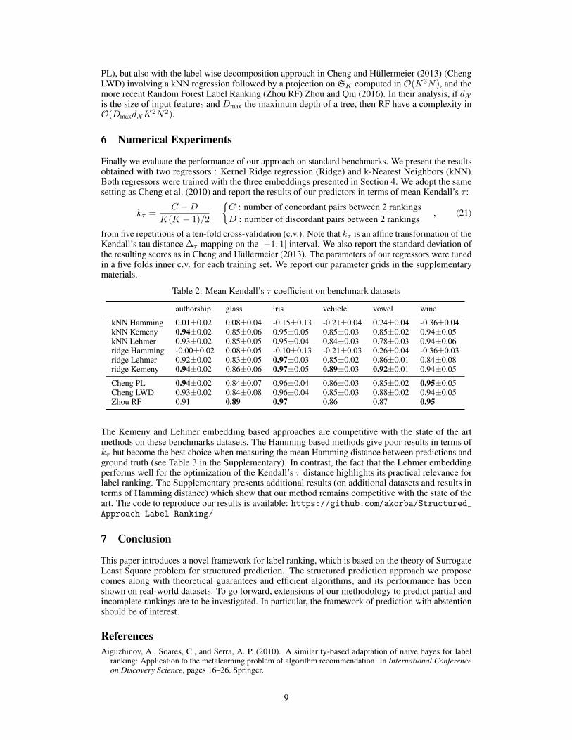
Table 2: Mean Kendall’s τ coefficient on benchmark datasets

authorship glass iris vehicle vowel wine

kNN Hamming 0.01±0.02 0.08±0.04 -0.15±0.13 -0.21±0.04 0.24±0.04 -0.36±0.04kNN Kemeny 0.94±0.02 0.85±0.06 0.95±0.05 0.85±0.03 0.85±0.02 0.94±0.05kNN Lehmer 0.93±0.02 0.85±0.05 0.95±0.04 0.84±0.03 0.78±0.03 0.94±0.06ridge Hamming -0.00±0.02 0.08±0.05 -0.10±0.13 -0.21±0.03 0.26±0.04 -0.36±0.03ridge Lehmer 0.92±0.02 0.83±0.05 0.97±0.03 0.85±0.02 0.86±0.01 0.84±0.08ridge Kemeny 0.94±0.02 0.86±0.06 0.97±0.05 0.89±0.03 0.92±0.01 0.94±0.05

Cheng PL 0.94±0.02 0.84±0.07 0.96±0.04 0.86±0.03 0.85±0.02 0.95±0.05Cheng LWD 0.93±0.02 0.84±0.08 0.96±0.04 0.85±0.03 0.88±0.02 0.94±0.05Zhou RF 0.91 0.89 0.97 0.86 0.87 0.95

The Kemeny and Lehmer embedding based approaches are competitive with the state of the artmethods on these benchmarks datasets. The Hamming based methods give poor results in terms ofkτ but become the best choice when measuring the mean Hamming distance between predictions andground truth (see Table 3 in the Supplementary). In contrast, the fact that the Lehmer embeddingperforms well for the optimization of the Kendall’s τ distance highlights its practical relevance forlabel ranking. The Supplementary presents additional results (on additional datasets and results interms of Hamming distance) which show that our method remains competitive with the state of theart. The code to reproduce our results is available: https://github.com/akorba/Structured_Approach_Label_Ranking/

7 Conclusion

This paper introduces a novel framework for label ranking, which is based on the theory of SurrogateLeast Square problem for structured prediction. The structured prediction approach we proposecomes along with theoretical guarantees and efficient algorithms, and its performance has beenshown on real-world datasets. To go forward, extensions of our methodology to predict partial andincomplete rankings are to be investigated. In particular, the framework of prediction with abstentionshould be of interest.

ReferencesAiguzhinov, A., Soares, C., and Serra, A. P. (2010). A similarity-based adaptation of naive bayes for label

ranking: Application to the metalearning problem of algorithm recommendation. In International Conferenceon Discovery Science, pages 16–26. Springer.

9

Ailon, N. (2010). Aggregation of partial rankings, p-ratings and top-m lists. Algorithmica, 57(2):284–300.

Aledo, J. A., Gámez, J. A., and Molina, D. (2017). Tackling the supervised label ranking problem by baggingweak learners. Information Fusion, 35:38–50.

Brazdil, P. B., Soares, C., and Da Costa, J. P. (2003). Ranking learning algorithms: Using ibl and meta-learningon accuracy and time results. Machine Learning, 50(3):251–277.

Brouard, C., Szafranski, M., and d?Alché Buc, F. (2016). Input output kernel regression: supervised andsemi-supervised structured output prediction with operator-valued kernels. Journal of Machine LearningResearch, 17(176):1–48.

Calauzenes, C., Usunier, N., and Gallinari, P. (2012). On the (non-) existence of convex, calibrated surrogatelosses for ranking. In Advances in Neural Information Processing Systems, pages 197–205.

Cao, Z., Qin, T., Liu, T.-Y., Tsai, M.-F., and Li, H. (2007). Learning to rank: from pairwise approach to listwiseapproach. In Proceedings of the 24th Annual International Conference on Machine learning (ICML-07),pages 129–136. ACM.

Caponnetto, A. and De Vito, E. (2007). Optimal rates for the regularized least-squares algorithm. Foundationsof Computational Mathematics, 7(3):331–368.

Cheng, W., Hühn, J., and Hüllermeier, E. (2009). Decision tree and instance-based learning for label ranking. InProceedings of the 26th Annual International Conference on Machine Learning (ICML-09), pages 161–168.ACM.

Cheng, W. and Hüllermeier, E. (2013). A nearest neighbor approach to label ranking based on generalizedlabelwise loss minimization.

Cheng, W., Hüllermeier, E., and Dembczynski, K. J. (2010). Label ranking methods based on the plackett-lucemodel. In Proceedings of the 27th Annual International Conference on Machine Learning (ICML-10), pages215–222.

Chiang, T.-H., Lo, H.-Y., and Lin, S.-D. (2012). A ranking-based knn approach for multi-label classification. InAsian Conference on Machine Learning, pages 81–96.

Ciliberto, C., Rosasco, L., and Rudi, A. (2016). A consistent regularization approach for structured prediction.In Advances in Neural Information Processing Systems, pages 4412–4420.

Clémençon, S., Korba, A., and Sibony, E. (2017). Ranking median regression: Learning to order through localconsensus. arXiv preprint arXiv:1711.00070.

Cortes, C., Mohri, M., and Weston, J. (2005). A general regression technique for learning transductions. InProceedings of the 22nd Annual International Conference on Machine learning (ICML-05), pages 153–160.

de Sá, C. R., Azevedo, P., Soares, C., Jorge, A. M., and Knobbe, A. (2018). Preference rules for label ranking:Mining patterns in multi-target relations. Information Fusion, 40:112–125.

Dekel, O., Singer, Y., and Manning, C. D. (2004). Log-linear models for label ranking. In Advances in neuralinformation processing systems, pages 497–504.

Devroye, L., Györfi, L., and Lugosi, G. (2013). A probabilistic theory of pattern recognition, volume 31.Springer Science & Business Media.

Deza, M. and Deza, E. (2009). Encyclopedia of Distances. Springer.

Djuric, N., Grbovic, M., Radosavljevic, V., Bhamidipati, N., and Vucetic, S. (2014). Non-linear label ranking forlarge-scale prediction of long-term user interests. In AAAI, pages 1788–1794.

Fagin, R., Kumar, R., Mahdian, M., Sivakumar, D., and Vee, E. (2004). Comparing and aggregating rankingswith ties. In Proceedings of the twenty-third ACM SIGMOD-SIGACT-SIGART symposium on Principles ofdatabase systems, pages 47–58. ACM.

Fathony, R., Behpour, S., Zhang, X., and Ziebart, B. (2018). Efficient and consistent adversarial bipartitematching. In International Conference on Machine Learning, pages 1456–1465.

Fürnkranz, J. and Hüllermeier, E. (2003). Pairwise preference learning and ranking. In European conference onmachine learning, pages 145–156. Springer.

10

Geng, X. and Luo, L. (2014). Multilabel ranking with inconsistent rankers. In Computer Vision and PatternRecognition (CVPR), 2014 IEEE Conference on, pages 3742–3747. IEEE.

Gurrieri, M., Siebert, X., Fortemps, P., Greco, S., and Słowinski, R. (2012). Label ranking: A new rule-basedlabel ranking method. In International Conference on Information Processing and Management of Uncertaintyin Knowledge-Based Systems, pages 613–623. Springer.

Jiao, Y., Korba, A., and Sibony, E. (2016). Controlling the distance to a kemeny consensus without computingit. In Proceedings of the 33rd Annual International Conference on Machine learning (ICML-16), pages2971–2980.

Kadri, H., Ghavamzadeh, M., and Preux, P. (2013). A generalized kernel approach to structured output learning.In Proceedings of the 30th Annual International Conference on Machine learning (ICML-13), pages 471–479.

Kamishima, T., Kazawa, H., and Akaho, S. (2010). A survey and empirical comparison of object rankingmethods. In Preference learning, pages 181–201. Springer.

Kenkre, S., Khan, A., and Pandit, V. (2011). On discovering bucket orders from preference data. In Proceedingsof the 2011 SIAM International Conference on Data Mining, pages 872–883. SIAM.

Kuhn, H. W. (1955). The hungarian method for the assignment problem. Naval Research Logistics (NRL),2(1-2):83–97.

Li, P., Mazumdar, A., and Milenkovic, O. (2017). Efficient rank aggregation via lehmer codes. arXiv preprintarXiv:1701.09083.

Mareš, M. and Straka, M. (2007). Linear-time ranking of permutations. In European Symposium on Algorithms,pages 187–193. Springer.

Merlin, V. R. and Saari, D. G. (1997). Copeland method ii: Manipulation, monotonicity, and paradoxes. Journalof Economic Theory, 72(1):148–172.

Micchelli, C. A. and Pontil, M. (2005). Learning the kernel function via regularization. Journal of machinelearning research, 6(Jul):1099–1125.

Myrvold, W. and Ruskey, F. (2001). Ranking and unranking permutations in linear time. Information ProcessingLetters, 79(6):281–284.

Nowozin, S. and Lampert, C. H. (2011). Structured learning and prediction in computer vision. Found. Trends.Comput. Graph. Vis., 6(3:8211;4):185–365.

Osokin, A., Bach, F. R., and Lacoste-Julien, S. (2017). On structured prediction theory with calibrated convexsurrogate losses. In Advances in Neural Information Processing Systems (NIPS) 2017, pages 301–312.

Ramaswamy, H. G., Agarwal, S., and Tewari, A. (2013). Convex calibrated surrogates for low-rank loss matriceswith applications to subset ranking losses. In Advances in Neural Information Processing Systems, pages1475–1483.

Sá, C. R., Soares, C. M., Knobbe, A., and Cortez, P. (2017). Label ranking forests.

Steinwart, I. and Christmann, A. (2008). Support Vector Machines. Springer.

Vembu, S. and Gärtner, T. (2010). Label ranking algorithms: A survey. In Preference learning, pages 45–64.Springer.

Wang, D., Mazumdar, A., and Wornell, G. W. (2015). Compression in the space of permutations. IEEETransactions on Information Theory, 61(12):6417–6431.

Wang, Q., Wu, O., Hu, W., Yang, J., and Li, W. (2011). Ranking social emotions by learning listwise preference.In Pattern Recognition (ACPR), 2011 First Asian Conference on, pages 164–168. IEEE.

Yu, P. L. H., Wan, W. M., and Lee, P. H. (2010). Preference Learning, chapter Decision tree modelling forranking data, pages 83–106. Springer, New York.

Zhang, M.-L. and Zhou, Z.-H. (2007). Ml-knn: A lazy learning approach to multi-label learning. Patternrecognition, 40(7):2038–2048.

Zhou, Y., Liu, Y., Yang, J., He, X., and Liu, L. (2014). A taxonomy of label ranking algorithms. JCP,9(3):557–565.

Zhou, Y. and Qiu, G. (2016). Random forest for label ranking. arXiv preprint arXiv:1608.07710.

11