A stochastic mimo radio channel model with …grouper.ieee.org/groups/802/20/DropBox/Kermoal_JSAC_2002... · A Stochastic MIMO Radio Channel Model With Experimental Validation ...

IEEE JOURNAL ON SELECTED AREAS IN COMMUNICATIONS, VOL. 20, NO. 6, AUGUST 2002 1211

A Stochastic MIMO Radio Channel ModelWith Experimental Validation

Jean Philippe Kermoal, Laurent Schumacher, Member, IEEE, Klaus Ingemann Pedersen, Member, IEEE,Preben Elgaard Mogensen, Member, IEEE, and Frank Frederiksen

Abstract—Theoretical and experimental studies of mul-tiple-input/multiple-output (MIMO) radio channels are presentedin this paper. A simple stochastic MIMO model channel has beendeveloped. This model uses the correlation matrices at the mobilestation (MS) and base station (BS) so that results of the numeroussingle-input/multiple-output studies that have been published inthe literature can be used as input parameters. In this paper, themodel is simplified to the narrowband channels. The validationof the model is based upon data collected in both picocell andmicrocell environments. The stochastic model has also been usedto investigate the capacity of MIMO radio channels, consideringtwo different power allocation strategies, water filling and uniformand two different antenna topologies, 4 4 and 2 4. Spacediversity used at both ends of the MIMO radio link is shownto be an efficient technique in picocell environments, achievingcapacities within 14 b/s/Hz and 16 b/s/Hz in 80% of the cases for a4 4 antenna configuration implementing water filling at a SNRof 20 dB.

Index Terms—Eigenanalysis, multiple-input/multiple-outputmeasurement, spectral efficiency, stochastic multiple-input/mul-tiple-output radio channel model.

I. INTRODUCTION

T HE REMARKABLE Shannon capacity available from de-ploying multiple antennas at both the transmitter (Tx) and

the receiver (Rx) of a wireless system, has generated consider-able interest in recent years [1], [2]. Large capacity is obtainedvia the potential decorrelation between the channel coefficientof the multiple-input/multiple-output (MIMO) radio channel,which can be exploited to create several parallel subchannels.However, the potential capacity gain is highly dependent on themultipath richness, since a fully correlated MIMO radio channelonly offers one subchannel, while a completely decorrelatedradio channel potentially offers multiple subchannels dependingon the antenna configuration.

Following Telatar’s seminal paper [3], most MIMO theoret-ical and simulation studies have assumed either fully correlatedor fully decorrelated radio channels [1], [4], while a partially

Manuscript received March 15, 2001; revised February 22, 2002. This workwas supported in part by the European Union IST Research Project METRA(Multi Element Transmit and Receive Antennas).

J. P. Kermoal and L. Schumacher are with the Center for PersonKom-munikation, Niels Jernes Vej 12, DK-9220 Aalborg East, Denmark (e-mail:[email protected]; [email protected]).

K. I. Pedersen and F. Frederiksen are with Nokia Networks, Niels JernesVej 10, DK-9220 Aalborg East, Denmark (e-mail: [email protected];[email protected]).

P. E. Mogensen is with the Center for PersonKommunikation, Niels Jernes Vej12 DK-9220 Aalborg East, Denmark and also with the Nokia Networks, NielsJernes Vej 10, DK-9220 Aalborg East, Denmark (e-mail: [email protected]).

Publisher Item Identifier 10.1109/JSAC.2002.801223.

correlated radio channel should be expected in practice. The ob-jective of this study is, therefore, to derive and to empiricallyvalidate a simple MIMO radio channel model, which is appli-cable for link level simulations. Some authors, as in [5], haveapproached the problem from a geometrically-based perspec-tive. In [5, p. 19], spatial fading correlation is introduced byextending the one-ring model of scatterers first used by Clarke[6, p. 60] to MIMO setups. A mathematical framework for asimple stochastic wideband MIMO radio channel model waspresented in [7]. In this paper, we simplify the model by refor-mulating it for narrowband (NB) channels.

One of the main strengths of the proposed MIMO stochasticmodel is that it relies on a small set of parameters to fully char-acterize the communication scenario, namely the power gain ofthe MIMO channel matrix, two correlation matrices describingthe correlation properties at both ends of the transmission links,and the associated Doppler spectrum of the channel paths.These parameters can be extracted from measurement results,but they can also be derived from single-input/multiple-output(SIMO) results already published in the open literature. Indeed,during the last decade, many studies have focused on SIMOradio channel models for the evaluation of adaptive antennasat the base station (BS) [8]–[12]. These models have mainlybeen derived from geometric scattering distributions [9], [10]or extensive analysis of measurement data [11], [12].

The validation of the model is supported by measurement re-sults. Using two measurement setups exhibiting several transmitand receive elements, 107 paths, i.e., the radio link between thearray at the mobile station (MS) and BS, have been investigatedin seven different picocell and microcell environments. Param-eters of the MIMO model are extracted from the measurementdata and fed to the model such as to compare simulation resultswith the measurement results.

The paper is organized as follows. Section II introduces thestochastic MIMO radio channel model. In Section III, extensiveMIMO measurement campaigns are presented, followed by theexperimental validation of the stochastic model in Section IV.Finally, Section V presents capacity results in a single-user sce-nario based on simulated data generated by the proposed MIMOradio channel.

II. STOCHASTIC MIMO CHANNEL MODEL

A. General Description

Consider the MIMO setup pictured in Fig. 1 withantennas at the BS and antennas at the MS. Thesignals at the BS antenna array are denoted by the vector

0733-8716/02$17.00 © 2002 IEEE

1212 IEEE JOURNAL ON SELECTED AREAS IN COMMUNICATIONS, VOL. 20, NO. 6, AUGUST 2002

Fig. 1. Two antenna arrays in a scattering environment.

, where is the signal atthe th antenna port and denotes transposition. Similarly,the signals at the MS are .

A functional sketch of the MIMO radio channel is given inFig. 3. The NB MIMO radio channel which de-scribes the connection between the MS and the BS can be ex-pressed as

......

......

(1)

where is the complex transmission coefficient from an-tenna at the MS to antenna at the BS. For simplicity, it is as-sumed that is complex Gaussian distributed with identicalaverage power. However, this latest assumption can be easily re-laxed as shown in the Appendix. Thus, the relation between thevectors and can be expressed as

(2)

B. Assumptions

It is assumed that all antenna elements in the two arrays havethe same polarization and the same radiation pattern. The spatialcomplex correlation coefficient at the BS between antennaand is given by

(3)

where computes the correlation coefficient betweenand. From (3), it is assumed that the spatial correlation coefficient

at the BS is independent of, since the elements at the MS,illuminate the same surrounding scatterers and, therefore, alsogenerate the same power azimuth spectrum (PAS) at the BS. Re-call that the spatial correlation function is the Fourier transformof the PAS as discussed in [13]. Expressions of the spatial cor-relation function have been derived in the literature assumingthat the PAS follows a cosine raised to an even integer [14], aGaussian function [15], a uniform function [16], and a Laplacianfunction [17].

The spatial complex correlation coefficient observed at theMS is similarly defined as

(4)

and assumed to be independent of. An approximate expres-sion of the spatial correlation function averaged over all possibleazimuth orientations of the MS array is derived in [19]. It ap-pears as a function of the azimuth dispersionwith ,where 0 corresponds to a scenario where the power iscoming from one distinct direction only, while 1 whenthe PAS is uniformly distributed over the azimuthal range [0;360 ][18]. As the MS is typically nonstationary, the results pre-sented in [19] are considered to be very useful since they areaveraged over all orientations of the MS array.

Given (3) and (4), one can define the following symmetricalcomplex correlation matrices

......

......

and

......

......

(5)

for later use.Finally, the correlation coefficient between two arbitrary

transmission coefficients connecting two different sets ofantennas is expressed as

(6)

which is shown in the Appendix to be equivalent to

(7)

provided that (3) and (4) are independent ofand , respec-tively. In other words, this means that the spatial correlation ma-trix of the MIMO radio channel is the Kronecker product of thespatial correlation matrix at the MS and the BS and is given by

(8)

where represents the Kronecker product. This has also beenconfirmed in [20].

C. Generation of Simulated Correlated Channel Coefficients

Correlated channel coefficients are generated fromzero-mean complex independent identically distributed (i.i.d.)random variables shaped by the desired Doppler spectrumsuch that

(9)

where andwhere the symmetrical map-

ping matrix results from the standard Cholesky factorizationof the matrix provided that is nonsin-gular [28]. Subsequently, the generation of the simulated MIMOchannel matrix can be deduced from the vector. Note thatthe correlation matrices and the Doppler spectrum cannot bechosen independently, as they are connected through the PASat the MS [21].

KERMOAL et al.: A STOCHASTIC MIMO RADIO CHANNEL MODEL WITH EXPERIMENTAL VALIDATION 1213

Fig. 2. Illustration of the two measurement setups.

D. Restriction to the Model

The pin hole [4] or keyhole [22] effect has been raised inprevious work. This effect would occur when scattering regionssurrounding both transmit and receive ends are separated by ascreen with a small hole in the middle. In this case, the receivedsignal between the antenna elements at both ends of the MIMOradio link are uncorrelated, but still would have low rank.Although data were collected in variety of environments, thepin hole or keyhole effect was not observed. Neither can themodel reproduce this effect. This is explained by the fact thatin [22] the transfer channel matrix is described as a dyad withone degree of freedom, where each channel coefficient writes asthe product of two independent zero-mean complex Gaussianrandom variables. It is, therefore, not possible to claim that alinear generation process as described in (9) can account for theproduct of random variables.

III. M EASUREMENTCAMPAIGNS

The objectives of the measurement campaigns described inthis section are to collect the data required to 1) validate theMIMO radio channel model and 2) estimate the model parame-ters that characterize different environments.

A. Measurement Setups

Two measurement setups are considered. They differ in themotion of the Tx and the antenna array topology of the Tx, as il-lustrated in Fig. 2 and described in [23] and [24]. In both setups,the Tx is at the MS and the stationary Rx is located at the BS.These two setups provide measurement results with differentcorrelation properties of the MIMO channel for small antennaspacings of the order of 0.5or 1.5 . The BS consists of fourparallel Rx channels. The sounding signal is a MSK-modulatedlinear shift register sequence of a length of 127 chips, clockedat a chip rate of 4.096 Mcps. At the Rx, the channel soundingis performed within a window of 14.6s, with a sampling res-olution of 122 ns (1/2 chip period) to obtain an estimate of the

Fig. 3. Functional sketch of the MIMO model.d stands for distancebetween MS and BS,h for the height of BS above ground floor, and AS forazimuth spread.

Fig. 4. Second measurement setup. The MS appears on the foreground withthe “satellite” and its shield while the BS stands in the background.

complex impulse response (IR). The NB information is subse-quently extracted by averaging the complex delayed signal com-ponents. A more thorough description of the stand-alone testbed(i.e., Rx and Tx) is documented in [25].

1) First Measurement Setup:A standard vertically polar-ized dipole antenna (Fig. 3) is mounted on a rotating bar anddescribes a circumferential distance of 20where is thewavelength. The operating frequency is 1.71 GHz. A syn-thesized antenna array with a separation of 0.5between theantenna elements is considered in the post-processing analysis.A uniform linear antenna array with four elements polarized at

45 spaced by 0.45 is used at the BS.2) Second Measurement Setup:An interleaved antenna

array with four vertically polarized sleeve dipoles elementsmounted at the MS is moved along a linear slide over a distanceof 11.8 as shown in Fig. 4. Such an antenna arrangement isdescribed in detail in [24] and is used to reduce the mutual


TABLE ISUMMARY AND DESCRIPTION OF THEDIFFERENTMEASUREDENVIRONMENTS

coupling between the elements, thus, preserving the omnidi-rectionality of the radiation pattern of the antenna elements.After post processing, a linear array is derived from it with aspacing of 0.4. The Tx uses a 1-to-4 switch with a switchinterval of 50 s between each element of the antenna array,implementing a pseudo parallel transmission within 200s.Note, the operating frequency is 2.05 GHz (UMTS band)for this setup. At the BS, a uniform linear array with fourvertically polarized sleeve dipoles elements with a spacing of1.5 is employed. The MS consists of two trolleys where onetrolley contains all the electronic hardware of the Tx and theother, later referred to as the “satellite,” is equipped with thelinear slide carrying the Tx antenna array. The two trolleys areconnected by 10-m coaxial and signal cables. The purpose ofusing two trolleys is to reduce the effect of reflections frommetallic surfaces. The satellite trolley is made of wood andthe metallic part of the linear slide is shielded by microwaveabsorbers as shown in Fig. 4.

B. Environment

Channel data were collected in two types of environments:picocell and microcell. Here the term picocell and microcellrefer to indoor-to-indoor and indoor-to-outdoor environment,respectively. The measurement campaigns are undertaken inseveral buildings at two main locations: the campus of AalborgUniversity and the Aalborg International Airport. Table Isummarizes the environments.

For each environment (A–G), several MS locations are se-lected to provide a set of measurements where both line-of-sight(LOS) and non-LOS (NLOS) scenarios are present. Moreover,several BS locations are selected within the same environmentin addition to the MS locations, as illustrated in Fig. 5, in orderto increase the reachness of the data set. A total of 107 paths areinvestigated within these seven environments.

The first measurement setup is used to investigate 15 pathsin a microcell environment, i.e., environment A in Table I. TheMS is positioned in different locations inside a building whilethe BS is mounted on a crane and elevated above roof top level(i.e., 9 m) to provide direct LOS to the building. The antenna is

Fig. 5. Example of picocell environment C. The arrows represent thedisplacement of the MS (1 to 7). The three shaded areas represent the differentpositions of the BS, with the circles illustrating each antenna element of thearray. In total, 21 paths are investigated for this environment.

located 300 m away from the building. The second setup is usedto investigate 92 paths for both microcell and picocell environ-ments, i.e., environment B and C to G, respectively, as shown inTable I. The distance between the BS and the MS is 31 to 36 mfor microcell B, with the BS located outside.

The stochastic model relies on the wide sense stationary(WSS) condition, meaning that as a rule of thumb the scatterersshould be 10 times the distance travelled by the MS awayfrom it, which is equivalent to about 20 m in the present case.This condition can be questionable when considering practicalmeasurements. Indeed, when measurements were undertakenin small rooms, the travelled distance of the MS was verysimilar to the distance of the MS to the wall, hence possiblynot fulfilling the WSS condition. These restrictions need tobe considered when discussing the validity of the simulatedresults.

IV. M ODEL VALIDATION

The purpose of this section is four-fold: 1) to validate that theassumptions stated in the presented model apply to the measureddata; 2) to introduce the input parameters used to validate themodel; 3) to present the eigenanalysis used as benchmark inthis validation process and, finally, 4) to illustrate the validationprocedure and its outcome.


Fig. 6. Example of the cdf ofstd � (left graph) andstd � (rightgraph). The cdf is performed over all the measured environments and for all theseven correlation coefficients.

A. Validation of the Stochastic MIMO Channel ModelAssumptions

The validity of the underlying assumptions has been verifiedfor a 4 4 MIMO configuration. These assumptions are that1) the spatial correlation at the BS (3) and the MS (4) is inde-pendent of and , respectively, and 2) the spatial correlationmatrix of the MIMO radio channel is the Kronecker product ofthe spatial correlation matrices at the BS and the MS (8).

Assumption 1):The standard deviation (std) of each mea-sured spatial correlation coefficient and iscomputed over the and reference antennas, respectively,for each environment. The std at the BS is expressed as

and at the MS such that

Fig. 6 presents the empirical cumulative distribution function(cdf) of (left graph) and (right graph) com-puted over the 92 paths considered with the second measure-ment setup for the six different correlation coefficients, i.e., theupper triangular coefficient of the correlation matrix, when a4 4 MIMO configuration is used. To validate the statisticalsignificance of the empirical results, the empirical cdf is com-pared with a cdf obtained from simulations performed undersimilar conditions. The matching of the two cdfs demonstratesthat Assumption 1) is fulfilled, as explained here after.

For each of the 92 6 different measured correlation coef-ficients, two correlated, Rayleigh-distributed signals of length1000 are generated. These 1000-long vectors are truncatedinto 11.8 -long runs over which the correlation coefficient iscomputed once again. Hence, a wider new set of correlationvalues is collected, exhibiting a standard deviation std. Thisoperation is repeated 926 times. A simulated cdf of stdis then obtained under similar conditions than the measured cdf.

However, these two cdfs could differ in two ways. Since thesimulated cdf has been computed from a larger set of statisticsthan the measured cdf, it could exhibit a steeper slope. On theother hand, should Assumption 1) not be fulfilled, the medianpoint of the cdfs would not coincide.

The simulated cdf is shown in Fig. 6. The slope difference ofthese cdfs indicates the impact of the lack of measured statisticswith respect to the simulations described here above. But thefairly good match between the measured and the simulated cdfssupports assumption (3) and (4).

Assumption 2):This assumption is validated by comparingresults generated from the proposed MIMO radio channel modelwith measured data. This is presented in Section IV-D.

B. Input Parameters to the Validation of the MIMO Model

The input parameters used in the validation stage are illus-trated by the shaded area of Fig. 3. They are 1) the average spa-tial complex correlation matrices and and 2) the as-sociated average Doppler spectrum.

The measured spatial complex correlation matrices are theresults of an average over the reference antennasand withrespect to which the matrices are computed.

The averaged measured Doppler spectrum is obtained by av-eraging over all the channel coefficients. It is defined atthe MS, since the BS is fixed. This limitation is due to the mea-surement setup implementation, but is not inherent to the model.If both MS and BS were moving, the Doppler spectrum of thechannels would have been defined as the convolution of sepa-rate Doppler spectra defined either at the MS or at the BS, con-sidering, respectively, the BS and the MS as fixed.1 The cor-responding complex coefficients of the vector(9) have theiramplitudes shaped by the average measured Doppler spectrumand assigned a random phase uniformly distributed over [0, 2]such that independent and identically distributed variablesare generated.

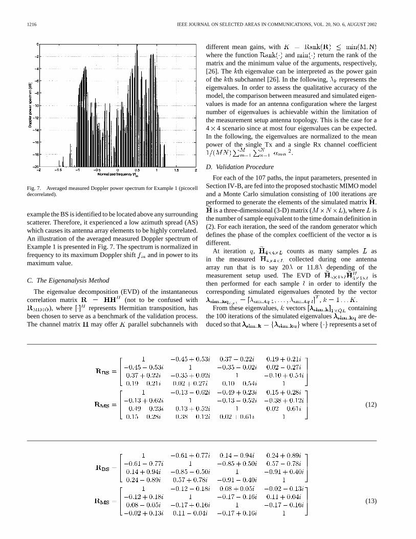
Two examples of typical paths have been selected from theset of paths described in Section III. Their differences in termsof propagation properties motivated this choice. Example 1 isone of the paths in the picocell environment C where the prop-agation scenario offers a decorrelated case. On the other hand,example 2 presents the opposite situation where the propagationscenario is correlated. This appears in one of the paths in the mi-crocell environment A.

Example 1: Picocell Decorrelated.See (12) at the bottom of the next page.Example 2: Microcell Correlated.See (13) at the bottom of the next page.Both in Example 1 and 2, is decorrelated. This is ex-

pected since the MS is surrounded by scatterers. On the otherhand, presents two different behaviors. In Example 1,the spatial correlation coefficients remain low as expected in thecase of an indoor termination. On the other hand, the spatial cor-relation coefficients at the BS are highly correlated in Example 2with a mean absolute value of the coefficient of 0.96. The highcorrelation is explained by the fact that regarding this specific

1The phase shifts due to both movements add, causing the respective phasersto multiply each other, which is equivalent to the convolution of their Dopplerspectra.


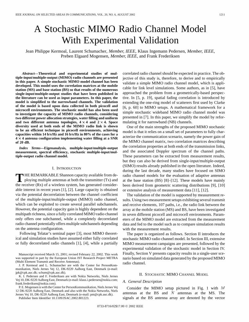
Fig. 7. Averaged measured Doppler power spectrum for Example 1 (picocelldecorrelated).

example the BS is identified to be located above any surroundingscatterer. Therefore, it experienced a low azimuth spread (AS)which causes its antenna array elements to be highly correlated.An illustration of the averaged measured Doppler spectrum ofExample 1 is presented in Fig. 7. The spectrum is normalized infrequency to its maximum Doppler shift and in power to itsmaximum value.

C. The Eigenanalysis Method

The eigenvalue decomposition (EVD) of the instantaneouscorrelation matrix (not to be confused with

), where represents Hermitian transposition, hasbeen chosen to serve as a benchmark of the validation process.The channel matrix may offer parallel subchannels with

different mean gains, withwhere the function and return the rank of thematrix and the minimum value of the arguments, respectively,[26]. The th eigenvalue can be interpreted as the power gainof the th subchannel [26]. In the following, represents theeigenvalues. In order to assess the qualitative accuracy of themodel, the comparison between measured and simulated eigen-values is made for an antenna configuration where the largestnumber of eigenvalues is achievable within the limitation ofthe measurement setup antenna topology. This is the case for a4 4 scenario since at most four eigenvalues can be expected.In the following, the eigenvalues are normalized to the meanpower of the single Tx and a single Rx channel coefficient

.

D. Validation Procedure

For each of the 107 paths, the input parameters, presented inSection IV-B, are fed into the proposed stochastic MIMO modeland a Monte Carlo simulation consisting of 100 iterations areperformed to generate the elements of the simulated matrix.

is a three-dimensional (3-D) matrix ( ), where isthe number of sample equivalent to the time domain definition in(2). For each iteration, the seed of the random generator whichdefines the phase of the complex coefficient of the vectorisdifferent.

At iteration , counts as many samples asin the measured collected during one antennaarray run that is to say 20 or 11.8 depending of themeasurement setup used. The EVD of isthen performed for each samplein order to identify thecorresponding simulated eigenvalues denoted by the vector

, .From these eigenvalues,vectors containing

the 100 iterations of the simulated eigenvalues are de-duced so that where represents a set of

(12)

(13)


Fig. 8. Local validation. Cdf of� and� from Example 1 (picocelldecorrelated).

Fig. 9. Local validation. Cdf of� and � from Example 2(microcell correlated).

variables. For the measured data, the eigenvalues were deducedso that .

1) Local Validation: The local validation consists of thematching comparison between the cdf of andfor each of the 107 paths. Figs. 8 and 9 present the eigenanalysisperformed on the two propagation environments, Example1 and 2, respectively. The cdfs of the measured eigenvalues

for a full run of the Tx antenna array are displayedwith a solid line. On the same graph the cdfs of the simulatedeigenvalues are illustrated by a dashed line. Their cdfshave been performed over the variables of the vector

.Inspection of Figs. 8 and 9 reveals that the cdfs of the eigen-

values generated by the stochastic model closely match thoseestimated using measured data.

2) Global Validation: A global analysis encompassing allthe 107 paths has been performed in order to measure the differ-ence between the measured and the simulated results. The com-

Fig. 10. Global validation. Cdf ofj� j over the 107 paths.

parison is based on the difference between andat 50% ( .5 0.3) outage level for each paths and foreach eigenvalue such that .For more clarity in the graph, the absolute value isconsidered since is symmetrical around zero. Despitethe expected discrepancies between empirical and simulated re-sults, one can see from Fig. 10 that the error generated by theproposed model is bounded by0.6 dB for the strongest simu-lated eigenvalue , by 1.6 dB for , by 2.2 dB for

and by 2.7 dB for the weakest one, for 90% of the paths.These values are considered to be small error boundaries andit can be concluded that the proposed stochastic MIMO radiochannel model has been validated.

V. SPECTRAL EFFICIENCY—SINGLE-USERSCENARIO

This section investigates the spectral efficiency of MIMOchannels. This study is limited to single-user scenarios. Twopower allocation strategies are compared in the following, si-multaneously with two antenna array topologies.

A. Definition of the Power Allocation Schemes

In the situation where the channel is known at both Tx andRx and is used to compute the optimum weight, the power gainin the th subchannel is given by theth eigenvalue, i.e., thesignal-to-noise ratio (SNR) for theth subchannel equals

(14)

where is the power assigned to theth subchannel, is theth eigenvalue and is the noise power. For simplicity, it is

assumed that 1. According to Shannon, the maximumcapacity2 of parallel subchannels equals [26]

(15)

2The capacity expressions given throughout the paper are normalized withrespect to the bandwidth, i.e., they are given in terms of b/s/Hz (spectral effi-ciency).


Fig. 11. Cdf of the capacity per subchannelC and its total results C forExample 1 (picocell decorrelated). A 4� 4 antenna topology is presented here.

(16)

where the mean SNR is defined as

(17)

Given the set of eigenvalues , the power allocatedto each subchannel is determined to maximize the capacityby using Gallager’s water filling theorem [26] such that eachsubchannel is filled up to a common level, i.e.,

(18)

with a constraint on the total Tx power such that

(19)

where is the total transmitted power. This means that thesubchannel with the highest gain is allocated with the largestamount of power. In the case where then 0.

When the uniform power allocation scheme is employed, thepower is adjusted according to

(20)

Thus, in the situation where the channel is unknown, the uniformdistribution of the power is applicable over the antennas [26]so that the power should be equally distributed between theelements of the array at the Tx, i.e.,

(21)

B. Impact of the Orthogonal Subchannels on SpectralEfficiency

Fig. 11 illustrates the impact of each subchannel upon thetotal capacity available for a 4 4 antenna configuration inthe context of Example 1 at 20 dB. Here, is thecapacity of the th subchannel of Fig. 8. When looking at the

Fig. 12. Capacity (10% level) versus SNR for Example 1 (picocelldecorrelated) and Example 2 (microcell-correlated).

10% outage of Fig. 11, one can conclude that the total capacityis 17 b/s/Hz. This remarkable spectral efficiency is due

to the contribution of the significant , , and depictedin Fig. 8. From Fig. 11, one can also see that the differencebetween the two power allocation strategies is very small whenthe elements of the antenna array are sufficiently decorrelated[5, p. 64]. However, it must be emphasized that the water fillingscheme provides a higher capacity than the uniform powerdistribution.

C. Antenna Setup and SNR Impacts

Fig. 12 illustrates the total capacity from Fig. 11 at the 10%level for different SNRs when the water filling power alloca-tion scheme is used. Two antenna setups, a 44 and a 2 4,are compared. On the same figure, the decorrelated and the cor-related propagation scenarios are presented: Example 1 and 2.Three conclusions can be drawn from these examples.

1) One can see that the decorrelated situation provides morecapacity than the correlated one at the same SNR andgenerally the total capacity increases with the SNR.

2) In the decorrelated scenario (Example 1), the 44 an-tenna configuration takes full advantage of its additionalsubchannel compared with the 24.

3) The influence on the number of subchannels on the totalcapacity is illustrated for various SNRs. The capacityincreases in a linear manner as a function of the SNR ona log scale while the slope increase proportionally withthe number of subchannels in (15). At a low SNR, thecontribution of the strongest subchannel is predominant.For a higher SNR, all the subchannels contribute to thetotal capacity. As a consequence, one can see that for ahighSNR the slope of the 4 4 antenna array setup is twice theslope of the 2 4 one when comparing the two antennaarray configurations, since only two parallel subchannelsare achieved in the second antenna setup compared withthe four parallel subchannels achievable by the 44 one.This is an important observation, since it implies that 1) at


Fig. 13. Cdf over all the 79 (picocell) paths of the total capacity deduced fromFig. 12 atSNR = 20 dB for 4� 4 and 2� 4 antenna configuration.

low SNRs, the MIMO concept only provides a combinedTx and Rx diversity and 2) at high SNRs the MIMO systemoffers parallel channeling.

D. Spectral Efficiency Performance Per Cell Type

The capacity resulting from Fig. 12 and taken at a fixed SNRof 20 dB is extracted for all the 79 paths in picocell scenarioand its cdf is presented in Fig. 13. It is seen that the offeredcapacity is fairly constant for the picocell environments, sincethe capacity results equal 14 b/s/Hz and 16 b/s/Hz at the 10%and 90% outage levels, respectively. This is explained by thefact that the elements of the antenna arrays at both the BS andthe MS are sufficiently decorrelated in picocell (indoor to in-door) environments. In the context of a MIMO scenario this isinteresting since multiple parallel subchannels are available. Itcan, therefore, be concluded that, even in situations where LOSis present, a MIMO topology using space diversity with smallspacing is applicable for picocell environments.

Similarly to Fig. 13, Fig. 14 presents the cdf of the capacityderived from the 28 paths in the microcell scenario. One can seethat contrary to the scenario in Fig. 13, the estimated capacityexhibits a much larger variation. This is explained by the use oftwo different antenna spacings to estimate the input parameters.The capacity varying from 12 b/s/Hz to 16 b/s/Hz is attributedto the setup using 1.5while the low capacity contribution from9 to 12 b/s/Hz is obtained when applying only 0.5.

E. Consideration on the Spatial Domain in a MIMOPerspective

It is mentioned in [23] that when using 0.5separation atthe BS, the correlation between the elements of the antennaarray could vary from a correlated to a decorrelated situationwhich is explained by the fact that the BS experiences a lowAS, especially when positioned above surrounding scatterers,which cause its antenna elements to be highly correlated(Section IV-B, Example 2). On the other hand, when the ASbecomes larger, i.e., when the influence of the surroundingscatterers becomes more significant, the correlation betweenthe antenna array elements decreases.

Fig. 14. Cdf over all the 28 (microcell) paths of the total capacity deducedfrom Fig. 12 atSNR = 20 dB for 4� 4 and 2� 4 antenna configuration.

This highlights the fact that in microcell environments,the correlation is strongly influenced by the change in thesurrounding scatterers and also by the separation used in theantenna array. Therefore, the use of space diversity technique,on its own, is not recommended for a MIMO topology whenusing 0.5 antenna spacing at the BS. However, when 1.5isemployed, microcell capacity results indicate similar results asfor the picocell environment.

VI. CONCLUDING REMARKS

In this paper, a stochastic MIMO radio channel model hasbeen introduced and successfully validated in the NB condi-tion by comparing measured and simulated results. It has beenshown that the eigenvalues distribution of the model matches themeasurements. The advantage of the proposed model is that itsconfiguration, as far as time variation and spatial correlation areconcerned, can rely on SIMO results previously published in theopen literature. As such, it can be used for link-level simulationstudies, as illustrated by the derivation of theoretical capacitylimits. It is shown that space diversity used at both ends of theMIMO radio link is an efficient technique in picocell environ-ments, achieving capacities between 14 b/s/Hz and 16 b/s/Hzin 80% of the cases for a 44 antenna configuration imple-menting water-filling at a SNR of 20 dB.

APPENDIX

PROOF OF(7)

Consider the 2 2 correlated setup pictured in Fig. 15. Thecomplex correlation coefficients and are defined such as

(22)

(23)

(24)

(25)

where is the conjugate of .


Fig. 15. 2� 2 correlated setup.

On the other hand, the power correlation coefficient betweenantennas at the Tx is equal to . Similarly, the power correla-tion coefficient between the two receiving antenna elements isset to . In terms of channel transfer functions, this is givenby

(26)

(27)

(28)

(29)

Note that all these definitions assume that the correlation be-tween two given antenna elements at one end does not dependon the antenna used as a reference at the other end. This assump-tion is fulfilled if all antenna elements of a given end exhibit thesame radiation pattern.

Taking into account the fact that correlation matrices areHermitian [27, p. 101], the complex correlation matrices aredefined as follows:

(30)

(31)

Note that and can be replaced by andin up-link or and in down-link, respectively. Thepurpose of this Appendix is to demonstrate that correlatedchannel transfer functions can be generated from the Kroneckerproduct of the two complex correlation matrices. More partic-ularly, it aims at demonstrating that the complex correlationbetween channel coefficients and or, identically,between and , is the product of the antenna complexcorrelation coefficients and .

The Kronecker product of matrices (30) and (31) is given by

(32)

(33)

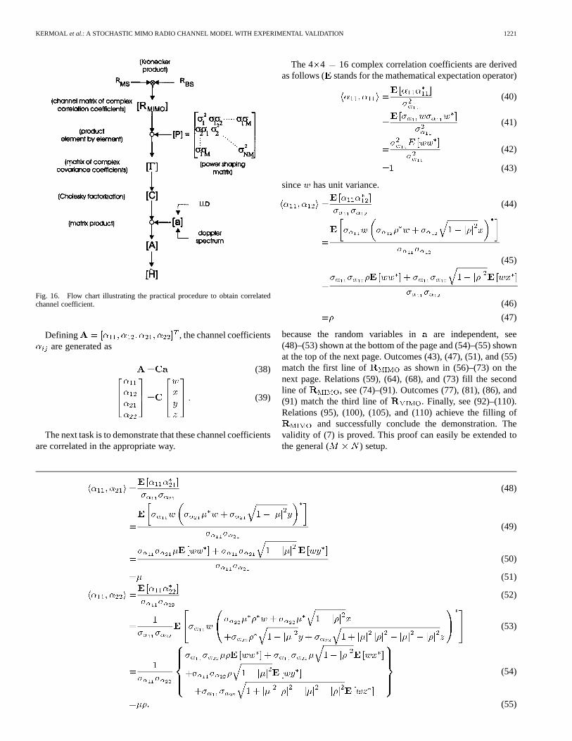
Let be a vector of four complex zero-mean,unit variance independent random variables. As described inSection II, correlated channel coefficients are generatedfrom the variable of the vector using the Cholesky decompo-sition of the matrix as illustrated in Fig. 16. results fromthe product of by a power-shaping matrix when anyimbalance in BPR (Branch Power Ratio) between antenna ele-ments occurs. The elements ofare the product of the standarddeviations of the channel coefficients . is given bythe following element-by-element product. See (34)–(36) at thebottom of the page.

Applying the Gaxpy algorithm [28, p. 143], the lower-trian-gular matrix , result of the Cholesky decomposition of, isgiven by (37) shown at the bottom of the page.

(34)

(35)

(36)

(37)


Fig. 16. Flow chart illustrating the practical procedure to obtain correlatedchannel coefficient.

Defining , the channel coefficientsare generated as

(38)

(39)

The next task is to demonstrate that these channel coefficientsare correlated in the appropriate way.

The 4 4 16 complex correlation coefficients are derivedas follows ( stands for the mathematical expectation operator)

(40)

(41)

(42)

(43)

since has unit variance.

(44)

(45)

(46)

(47)

because the random variables in are independent, see(48)–(53) shown at the bottom of the page and (54)–(55) shownat the top of the next page. Outcomes (43), (47), (51), and (55)match the first line of as shown in (56)–(73) on thenext page. Relations (59), (64), (68), and (73) fill the secondline of , see (74)–(91). Outcomes (77), (81), (86), and(91) match the third line of . Finally, see (92)–(110).Relations (95), (100), (105), and (110) achieve the filling of

and successfully conclude the demonstration. Thevalidity of (7) is proved. This proof can easily be extended tothe general ( ) setup.

(48)

(49)

(50)

(51)

(52)

(53)

(54)

(55)


(56)

(57)

(58)

(59)

(60)

(61)

(62)

(63)

(64)

(65)

(66)

(67)

(68)

(69)

(70)

(71)

(72)

(73)


(74)

(75)

(76)

(77)

(78)

(79)

(80)

(81)

(82)

(83)

(84)

(85)

(86)

(87)

(88)

(89)

(90)

(91)


(92)

(93)

(94)

(95)

(96)

(97)

(98)

(99)

(100)

(101)

(102)

(103)

(104)

(105)


(106)

(107)

(108)

(109)

(110)

ACKNOWLEDGMENT

The authors appreciate the useful comments from the anony-mous reviewers.

REFERENCES

[1] G. J. Foschini, “Layered space-time architecture for wireless communi-cation in fading environment when using multi-element antennas,”BellLabs Tech. J., pp. 41–59, Autumn 1996.

[2] G. G. Raleigh and J. M. Cioffi, “Spatio-temporal coding for wirelesscommunication,”IEEE Trans. Commun., vol. 46, pp. 357–366, Mar.1998.

[3] I. E. Telatar. (1995) Capacity of Multi-Antenna Gaussian Chan-nels. AT&T Bell Labs. [Online]. Available: http://mars.bell-labs.com/cm/ms/what/mars/papers/proof

[4] D. Gesbert, H. Boleskei, D. Gore, and A. Paulraj, “MIMO wireless chan-nels: Capacity and performance prediction,” inProc. GLOBECOM’00,vol. 2, San Francisco, USA, Nov. 2000, pp. 1083–1088.

[5] D. S. Shiu, Wireless Communication Using Dual AntennaArray. Norwell, MA: Kluwer, 2000.

[6] W. C. Jakes,Microwave Mobile Communications. New York: Wiley,1974.

[7] K. I. Pedersen, J. B. Andersen, J. P. Kermoal, and P. E. Mogensen, “Astochastic multiple-input multiple-output radio channel model for eval-uation of space-time coding algorithms,” inProc. Vehicular TechnologyConf., Boston, MA, Sept. 2000, pp. 893–897.

[8] R. B. Ertel, P. Cardieri, K. W. Sowerby, T. S. Rappaport, and J. H. Reed,“Overview of spatial channel models for antenna array communicationsystems,”IEEE Pers. Commun., pp. 10–21, Feb. 1998.

[9] J. Liberti and T. Rappaport, “A geometrically based model for line-of-sight multipath radio channels,” inProc. Vehicular Technology Conf.,Atlanta, Georgia, Apr. 1996, pp. 844–848.

[10] O. Nørklit and J. B. Andersen, “Diffuse channel model and experimentalresults for antenna arrays in mobile environments,”IEEE Trans. An-tennas Propagat., vol. 46, pp. 834–840, June 1998.

[11] P. Eggers, “Angular dispersive mobile radio environments sensed byhighly directive base station antennas,” inProc. PIMRC’95, Toronto,Canada, Sept. 1995, pp. 522–526.

[12] K. I. Pedersen and P. E. Mogensen, “Simulation of dual-polarized prop-agation environments for adaptive antennas,” inProc. Vehicular Tech-nology Conf., Amsterdam, Netherlands, Sept. 1999, pp. 62–66.

[13] B. H. Fleury, “First- and second-order characterization of direction dis-persion and space selectivity in the radio channel,”IEEE Trans. Inform.Theory, vol. 46, pp. 2027–2044, Sept. 2000.

[14] W. C. Y. Lee, “Effects on correlation between two mobile radio base-station antennas,”IEEE Trans. Commun., vol. 21, pp. 1214–1224, Nov.1973.

[15] F. Adachi, M. Feeny, A. Williamson, and J. Parsons, “Crosscorrelationbetween the envelopes of 900 MHz signals received at a mobile radiobase station site,”Proc. Inst. Elect. Eng., pt. F, vol. 133, pp. 506–512,Oct. 1986.

[16] J. Salz and J. Winters, “Effect of fading correlation on adaptive arrays indigital mobile radio,”IEEE Trans. Veh. Technol., vol. 43, pp. 1049–1057,Nov. 1994.

[17] K. I. Pedersen, P. E. Mogensen, and B. H. Fleury, “Spatial channelcharacteristics in outdoor environments and their impact on BS antennasystem performance,” inProc. Vehicular Technology Conf., Ottawa,Canada, May 1998, pp. 719–724.

[18] G. Durgin and T. S. Rappaport, “Basic relationship between multipathangular spread and narrowband fading in wireless channels,”Electron.Lett., vol. 34, pp. 2431–2432, Dec. 1998.


[19] , “Effects of multipath angular spread on the spatial cross-correla-tion of received voltage envelopes,” inProc. Vehicular Technolgy Conf.,Houston, TX, May 1999, pp. 996–1000.

[20] K. Yu, M. Bengtsson, B. Ottersten, D. McNamara, P. Karlsson, and M.Beach, “Second order statistics of NLOS indoor MIMO channels basedon 5.2 GHz measurements,” inProc. GLOBECOM’01, San Antonio,Texas, USA, Nov. 2001, pp. 156–160.

[21] P. Petrus, J. H. Reed, and T. S. Rappaport, “Effects of directional an-tennas at the base station on the Doppler spectrum,”IEEE Commun.Lett., vol. 1, pp. 40–42, Mar. 1997.

[22] D. Chizhik, G. J. Foschini, and R. A. Valenzuela, “Capacities of multi-el-ement transmit and receive antennas: Correlations and Keyholes,”Elec-tron. Lett., vol. 36, pp. 1099–1100, June 2000.

[23] J. P. Kermoal, P. E. Mogensen, S. H. Jensen, J. B. Andersen, F. Fred-eriksen, T. B. Sørensen, and K. I. Pedersen, “Experimental investigationof multipath richness for multi-element transmit and receive antenna ar-rays,” in Proc. Vehicular Technology Conf., Tokyo, Japan, May 2000,pp. 2004–2008.

[24] J. P. Kermoal, L. Schumacher, P. E. Mogensen, and K. I. Pedersen, “Ex-perimental investigation of correlation properties of MIMO radio chan-nels for indoor picocell scenarios,” inProc. Vehicular Technol.ogy Conf.,Boston, MA, Sept. 2000, pp. 14–21.

[25] F. Frederiksen, P. Mogensen, K. I. Pedersen, and P. Leth-Espensen, “A“Software” testbed for performance evaluation of adaptive antennas inFH GSM and wideband-CDMA,” inConf. Proc. 3rd ACTS Mobile Com-munication Summit, vol. 2, Rhodes, Greece, June 1998, pp. 430–435.

[26] J. B. Andersen, “Array gain and capacity for known random channelswith multiple element arrays at both ends,”IEEE J. Select. AreasCommun., vol. 18, pp. 2172–2178, Nov. 2000.

[27] S. Haykin,Adaptive Filter Theory. Upper Saddle River, NJ: Prentice-Hall, 1991.

[28] G. H. Golub and C. F. Van Loan,Matrix Computations, 3rded. Baltimore, MD: The Johns Hopkins Univ. Press, 1996.

Jean Philippe Kermoalwas born in Paris, France, in1972. He received the M.Phil. degree from the Uni-versity of Glamorgan, U.K., in 1998. He is currentlyworking towards the Ph.D. degree in multi-elementtransmit and receive antenna arrays for wireless com-munication systems at Aalborg University, Aalborg,Denmark.

His research interests include MIMO radio channelcharacterization, adaptive antenna array, and indoorand outdoor mobile communication propagation atmicrowave and millimeter-wave band.

Laurent Schumacher (M’96) was born in Mons,Belgium, in 1971. He received the M.Sc. E.E. degreefrom the Faculté Polytechnique de Mons, Belgium,in 1993 and the Ph.D. degree from the Universitécatholique de Louvain, Belgium, in 1999.

He then joined the Center for PersonKommunika-tion (CPK), Aalborg University, Aalborg, Denmark,where he has been appointed as Associate ResearchProfessor. His current research interests are the de-sign of MIMO radio channel models and the investi-gation of advanced algorithms and techniques for the

delivery of high bit-rate services in cellular systems (UMTS and beyond).

Klaus Ingemann Pedersen(S’97–M’00) receivedthe M.Sc. E.E. and Ph.D. degrees, in 1996 and 2000,respectively, from Aalborg University, Aalborg,Denmark.

He is currently with Nokia Networks, Aalborg,Denmark. His current research interests includeradio resource managements for WCDMA sys-tems, adaptive antenna array systems, and radiopropagation.

Preben Elgaard Mogensen(S’88–M’00) receivedthe M.Sc. E.E. and Ph.D. degrees, in 1988 and 1996,respectively, from Aalborg University, Aalborg,Denmark.

Since 1988, he has been with Aalborg University.He is currently holding a part time position asResearch Professor and heading the cellular SystemsResearch Group (CSYS) at the Center for Person-kommunikation (CPK). Since 1995, he has beenworking part time with Nokia Networks, Aalborg,Denmark, and is now Manager of the 3G Radio

Systems Research team at NET/Aalborg.

Frank Frederiksen received the M.Sc.E.E. degree intelecommunications from Aalborg University, Aal-borg, Denmark, in 1994.

From 1994 to 2000, he has been working at theCenter for Personkommunikation, Aalborg Univer-sity as a Research Engineer developing measurementsystems for DECT/GSM/W-CDMA. Since 2000, hehas been working for Nokia Networks, Aalborg, Den-mark, on evaluation of high speed data services forW-CDMA.

A stochastic mimo radio channel model with …grouper.ieee.org/groups/802/20/DropBox/Kermoal_JSAC_2002... · A Stochastic MIMO Radio Channel Model With Experimental Validation ...

Documents