A Stochastic Collocation Approach to Bayesian Inference in Inverse Problems

COMMUNICATIONS IN COMPUTATIONAL PHYSICSVol. 6, No. 4, pp. 826-847

Commun. Comput. Phys.October 2009

A Stochastic Collocation Approach to Bayesian

Inference in Inverse Problems

Youssef Marzouk1,∗ and Dongbin Xiu2

1 Department of Aeronautics & Astronautics, Massachusetts Institute of Technology,Cambridge, MA 02139, USA.2 Department of Mathematics, Purdue University, West Lafayette, IN 47907, USA.

Received 27 August 2008; Accepted (in revised version) 18 February 2009

Communicated by Jan S. Hesthaven

Available online 12 March 2009

Abstract. We present an efficient numerical strategy for the Bayesian solution of in-verse problems. Stochastic collocation methods, based on generalized polynomialchaos (gPC), are used to construct a polynomial approximation of the forward solu-tion over the support of the prior distribution. This approximation then defines a sur-rogate posterior probability density that can be evaluated repeatedly at minimal com-putational cost. The ability to simulate a large number of samples from the posteriordistribution results in very accurate estimates of the inverse solution and its associ-ated uncertainty. Combined with high accuracy of the gPC-based forward solver, thenew algorithm can provide great efficiency in practical applications. A rigorous erroranalysis of the algorithm is conducted, where we establish convergence of the approx-imate posterior to the true posterior and obtain an estimate of the convergence rate. Itis proved that fast (exponential) convergence of the gPC forward solution yields sim-ilarly fast (exponential) convergence of the posterior. The numerical strategy and thepredicted convergence rates are then demonstrated on nonlinear inverse problems ofvarying smoothness and dimension.

AMS subject classifications: 41A10, 60H35, 65C30, 65C50

Key words: Inverse problems, Bayesian inference, stochastic collocation, generalized polynomialchaos, uncertainty quantification.

1 Introduction

The indirect estimation of model parameters or inputs from observations constitutes aninverse problem. Such problems arise frequently in science and engineering, with applica-

∗Corresponding author. Email addresses: [email protected] (Y. Marzouk), [email protected] (D. Xiu)

http://www.global-sci.com/ 826 c©2009 Global-Science Press

Y. Marzouk and D. Xiu / Commun. Comput. Phys., 6 (2009), pp. 826-847 827

tions ranging from subsurface and atmospheric transport to chemical kinetics. In prac-tical settings, observations are inevitably noisy and may be limited in number or resolu-tion. Quantifying the resulting uncertainty in inputs or parameters is then essential forpredictive modeling and simulation-based decision-making.

The Bayesian approach to inverse problems [6,13,18,22,23] provides a foundation forinference from noisy and incomplete data, a natural mechanism for incorporating physi-cal constraints and heterogeneous sources of information, and a quantitative assessmentof uncertainty in the inverse solution. Indeed, the Bayesian setting casts the inverse solu-tion as a posterior probability distribution over the model parameters or inputs. Thoughconceptually straightforward, this setting presents challenges in practice; the posteriorprobability distribution is typically not of analytical form and, especially in high dimen-sions, cannot be easily interrogated. Many numerical approaches have been developedin response, mostly seeking to approximate the posterior distribution or posterior ex-pectations via samples [9]. These approaches require repeated solutions of the forwardmodel; when the model is computationally intensive, e.g., specified by partial differentialequations (PDEs), the Bayesian approach then becomes prohibitive.

Several efforts at accelerating Bayesian inference in inverse problems have appearedin recent literature; these have relied largely on reductions or surrogates for the forwardmodel [3, 14, 17, 24], or instead have sought more efficient sampling from the poste-rior [4,5,11]. Recent work [17] used (generalized) polynomial chaos (gPC)-based stochas-tic Galerkin methods [8, 29] to propagate prior uncertainty through the forward model,thus yielding a polynomial approximation of the forward solution over the support ofthe prior. This approximation then entered the likelihood function, resulting in a poste-rior density that was inexpensive to evaluate. This scheme was used to infer parametersappearing nonlinearly in a transient diffusion equation, demonstrating exponential con-vergence to the true posterior and multiple order-of-magnitude speedup in posterior ex-ploration via Markov chain Monte Carlo (MCMC). The gPC stochastic Galerkin approachhas also been extended to Bayesian inference of spatially-distributed quantities, such asinhomogeneous material properties appearing as coefficients in a PDE [16].

An alternative to the stochastic Galerkin approach to uncertainty propagation isstochastic collocation [25,27]. A key advantage of stochastic collocation is that it requiresonly a finite number of uncoupled deterministic simulations, with no reformulation ofthe governing equations of the forward model. Also, stochastic collocation can dealwith highly nonlinear problems that are challenging, if not impossible, to handle withstochastic Galerkin methods. A spectral representation may also be applied to arbitraryfunctionals of the forward solution; moreover, many methods exist for addressing highinput dimensionality via efficient low-degree integration formulae or sparse grids. Foran extensive discussion of gPC-based algorithms, see [26].

This paper extends the work of [17] by using gPC stochastic collocation to constructposterior surrogates for efficient Bayesian inference in inverse problems. We also con-duct a rigorous error analysis of the gPC Bayesian inverse scheme. Convergence of theapproximate posterior distribution to the true posterior distribution is established and

828 Y. Marzouk and D. Xiu / Commun. Comput. Phys., 6 (2009), pp. 826-847

its asymptotic convergence rate obtained. Numerical examples are provided for a vari-ety of nonlinear inverse problems to verify the theoretical findings and demonstrate theefficiency of the new algorithms.

2 Formulation

Let D⊂Rℓ, ℓ=1,2,3, be a physical domain with coordinates x=(x1,··· ,xℓ) and let T>0 be

a real number. We consider the following general stochastic partial differential equation

ut(x,t,Z)=L(u), D×(0,T]×Rnz ,

B(u)=0, ∂D×[0,T]×Rnz ,

u=u0, D×{t=0}×Rnz ,

(2.1)

where L is a (nonlinear) differential operator, B is the boundary condition operator, u0 isthe initial condition, and Z =(Z1,··· ,Znz)∈R

nz ,nz ≥ 1, are a set of independent randomvariables characterizing the random inputs to the governing equation. The solution istherefore a stochastic quantity,

u(x,t,Z) : D×[0,T]×Rnz →R

nu . (2.2)

We assume that each random variable Zi has a prior distribution

Fi(zi)= P(Zi ≤ zi)∈ [0,1],

where P denotes probability. In this paper we will focus on continuous random variables.Subsequently each Zi has a probability density function πi(zi) = dFi(zi)/dzi. The jointprior density function for Z is

πZ(z)=nz

∏i=1

πi(zi). (2.3)

Throughout this paper, we will neglect the subscript of each probability density and useπ(z) to denote the probability density function of the random variable Z, πZ(z), unlessconfusion arises otherwise. Note that it is possible to loosen the independence assump-tion on the input random variables Z by assuming some dependence structure; see, forexample, discussions in [1, 21]. As the focus of this paper is not on methods for thestochastic problem (2.1), we follow the usual approach by assuming prior independenceon Z.

Letdt = g(u)∈R

nd (2.4)

be a set of variables that one observes, where g : Rnu → R

nd is a function relating thesolution u to the true observable dt. We then define a “forward model” G : R

nz →Rnd to

describe the relation between the random parameters Z and observable dt:

dt =G(Z),g◦u(Z). (2.5)


In practice, measurement error is inevitable and the observed data d may not match thetrue value of dt. Assuming additive observational errors, we have

d=dt +e=G(Z)+e, (2.6)

where e∈Rnd are mutually independent random variables with probability density func-

tions π(e) = ∏ndi=1π(ei). We make the usual assumption that e are also independent of

Z.The present Bayesian inference problem is concerned with estimating the parameters

Z given a set of observations d. To this end, Bayes’ rule takes the form

π(z|d)=π(d|z)π(z)∫π(d|z)π(z)dz

, (2.7)

where π(z) is the prior probability density of Z; π(d|z) is the likelihood function; andπ(z|d), the density of Z conditioned on the data d, is the posterior probability density of Z.For notational convenience, we will use πd(z) to denote the posterior density π(z|d) andL(z) to denote the likelihood function π(d|z). That is, (2.7) can be written as

πd(z)=L(z)π(z)∫L(z)π(z)dz

. (2.8)

Following the independence assumption on the measurement noise e, the likelihoodfunction is

L(z),π(d|z)=nd

∏i=1

πei(di−Gi(z)). (2.9)

3 Algorithm

In this section we describe a stochastic collocation scheme, based on generalized polyno-mial chaos (gPC) expansions, for the Bayesian solution of the inverse problem (2.7).

3.1 Generalized polynomial chaos

The generalized polynomial chaos (gPC) is an orthogonal polynomial approximation torandom functions. Without loss of generality, in this subsection we describe the gPCapproximation to the forward problem (2.5) for nd =1. When nd >1 the procedure will beapplied to each component of G and is straightforward.

Let i = (i1,··· ,inz)∈ Nnz0 be a multi-index with |i|= i1+···+inz , and let N ≥ 0 be an

integer. The Nth-degree gPC expansion of G(Z) is defined as

GN(Z)=N

∑|i|=0

aiΦi(Z), (3.1)


where

ai =E[G(Z)Φi(Z)]=∫

G(z)Φi(z)π(z)dz, (3.2)

are the expansion coefficients, E is the expectation operator, and Φi(Z) are the basis func-tions defined as

Φi(Z)=φi1(Z1)···φinz(Znz), 0≤|i|≤N. (3.3)

Here φm(Zk) is the mth-degree one-dimensional orthogonal polynomial in the Zk direc-tion satisfying, for all k=1,··· ,nz,

Ek [φm(Zk)φn(Zk)]=∫

φm(zk)φn(zk)π(zk)dzk =δm,n, 0≤m,n≤N, (3.4)

where the expectation Ek is taken in terms of Zk only and the basis polynomials have beennormalized. Consequently {Φi(Z)} are nz-variate orthonormal polynomials of degree upto N satisfying

E[Φi(Z)Φj(Z)

]=

∫Φi(z)Φj(z)π(z)dz=δi,j , 0≤|i|,|j|≤N, (3.5)

where δi,j = ∏nz

k=1 δik,jk . From (3.4), the distribution of Zk will determine the polynomialtype. For example, Hermite polynomials are associated with the Gaussian distribution,Jacobi polynomials with the beta distribution, Laguerre polynomials with the gammadistribution, etc. For a detailed discussion of these correspondences and their resultingcomputational efficiency, see [28].

Following classical approximation theory, the gPC expansion (3.1) converges whenG(Z) is square integrable with respect to π(z), that is,

‖G(Z)−GN(Z)‖2L2

πZ,

∫(G(z)−GN(z))2π(z)dz→0, N→∞. (3.6)

Furthermore, the rate of convergence depends on the regularity of G such that

‖G(Z)−GN(Z)‖L2πZ≤CN−α, (3.7)

where C is a constant independent of N, and α > 0 depends on the smoothness of G.When G is relatively smooth, the convergence rate can be large. This implies that a rela-tively low-degree expansion can achieve high accuracy and is advantageous in practicalstochastic simulations. Many studies have been devoted to the convergence properties ofgPC, numerically or analytically, and the computational efficiency of gPC methods. See,for example, [2, 8, 15, 28, 29].

3.2 Stochastic collocation

In the pseudo-spectral stochastic collocation method [25], an approximate gPC expansionis sought, similar to (3.1), in the following form,

GN(Z)=N

∑|i|=0

aiΦi(Z), (3.8)


where the expansion coefficients are obtained by

ai =Q

∑m=1

G(Z(m))Φi(Z(m))w(m), (3.9)

where Z(m) =(Z(m)1 ,··· ,Z(m)

nz) are a set of nodes and w(m) are the corresponding weights

for m=1,··· ,Q, of an integration rule (cubature) on Rnz such that

ai ≈∫

G(z)Φi(z)π(z)dz= ai . (3.10)

The expansion of (3.8) thus becomes an approximation to the exact expansion (3.1); thatis,

GN(Z)≈GN(Z).

The difference between the two expansions is the so-called “aliasing error” [25] and isinduced by the error of using the integration rule in (3.9). If a convergent integration ruleis employed such that

limQ→∞

ai = ai, ∀i,

then

limQ→∞

GN(Z)=GN(Z), ∀Z, (3.11)

and convergence of GN to the exact forward model G follows naturally,

∥∥∥G(Z)−GN(Z)∥∥∥

2

L2πZ

→0, N→∞, Q→∞. (3.12)

A prominent feature of the pseudo-spectral collocation method is that it only requiressimulations of the forward model G(Z) at fixed nodes Z(m),m=1,··· ,Q, which are uncou-pled deterministic problems with different parameter settings. This significantly facili-tates its application in practical simulations, as long as the aliasing error is under control.For detailed presentation and analysis, see [25].

3.3 gPC-based Bayesian algorithm

In the gPC-based Bayesian method, we use the approximate gPC solution (3.8) to replacethe exact (but unknown) forward problem solution (3.1) in Bayes’ rule (2.8) and definethe following approximate posterior probability,

πdN(z)=

LN(z)π(z)∫LN(z)π(z)dz

, (3.13)


where π(z) is again the prior density of Z and LN is the approximate likelihood functiondefined as

LN(z), πN(d|z)=nd

∏i=1

πei(di−GN,i(z)), (3.14)

where GN,i is the i-th component of GN.

The advantage of this algorithm is that, upon obtaining an accurate gPC solution GN,dependence on the random parameters Z is known analytically (in polynomial form).Subsequently, the approximate posterior density πd

N of (3.13) can be evaluated at arbi-trary values of z and for an arbitrarily large number of samples, without resorting toadditional simulations of the forward problem. Very high accuracy in sampling the pos-terior distribution can thus be achieved at negligible computational cost. Combined withan efficient forward problem solver employing gPC collocation, this scheme provides afast and accurate method for Bayesian inference.

4 Convergence study

To establish convergence of the gPC-based Bayesian algorithm, we quantify the differ-ence between the approximate posterior πd

N and the exact posterior πd via Kullback-Leibler divergence. The Kullback-Leibler divergence (KLD) measures the difference be-tween probability distributions and is defined, for probability density functions π1(z)and π2(z), as

D(π1‖π2),∫

π1(z)logπ1(z)

π2(z)dz. (4.1)

It is always non-negative, and D(π1‖π2)=0 when π1 =π2.Similar to (3.13), we define πd

N as a posterior density obtained in terms of the exactNth-degree gPC expansion (3.1). That is,

πdN(z)=

LN(z)π(z)∫LN(z)π(z)dz

, (4.2)

where LN is the likelihood function obtained by using the exact Nth-degree gPC expan-sion (3.1),

LN(z),πN(d|Z)=nd

∏i=1

πei(di−GN,i(z)), (4.3)

where GN,i is the i-th component of GN . By the definitions of πdN and πd

N , we immediately

have the following lemma by following the pointwise convergence of GN to GN in (3.11).

Lemma 4.1. If GN converges to GN in the form of (3.11), i.e.,

limQ→∞

GN,i(Z)=GN,i(Z), 1≤ i≤nd, ∀Z, (4.4)


then

limQ→∞

πdN(z)=πd

N(z), ∀z, (4.5)

and

limQ→∞

D(

πdN‖πd

N

)=0. (4.6)

Hereafter we employ the common assumption that the observational error in (2.6) isi.i.d. Gaussian, and without loss of generality, assume

e∼N(0,σ2I), (4.7)

where σ>0 is the standard deviation and I is the identity matrix of size nd×nd.

Lemma 4.2. Assume that the observational error in (2.6) has an i.i.d. Gaussian distribution (4.7).If the gPC expansion GN (3.1) of the forward model converges to G in the form of (3.6), i.e.,

‖Gi(Z)−GN,i(Z)‖L2πZ

→0, 1≤ i≤nd, N→∞, (4.8)

then the posterior probability πdN (4.2) converges to the true posterior probability (2.8) in the sense

that the Kullback-Leibler divergence (4.1) converges to zero, i.e,

D(πdN‖πd)→0, N→∞. (4.9)

Proof. Let

γ=∫

L(z)π(z)dz, γN =∫

LN(z)π(z)dz. (4.10)

Obviously, γ > 0 and γN > 0. By following the definitions of the likelihood functionsL(z) (2.9) and LN(z) (4.3) and utilizing the fact that function e−x is (uniformly) Lipschitzcontinuous for x≥0, i.e., |e−x−e−y|≤Λ|x−y| for all x,y≥0, where Λ is a positive constant,we have

|γN−γ|=∣∣∣∣∫

(LN(z)−L(z))π(z)dz

∣∣∣∣

≤nd

∏i=1

∫1√

2πσ2

∣∣∣∣∣e− (di−GN,i (z))2

2σ2 −e− (di−Gi(z))2

2σ2

∣∣∣∣∣π(z)dz

≤nd

∏i=1

∫Λ

2σ2√

2πσ2

∣∣(di−GN,i(z))2−(di−Gi(z))2∣∣π(z)dz

≤nd

∏i=1

Λ

2σ2√

2πσ2‖GN,i−Gi‖L2

πZ‖2di−GN,i−Gi‖L2

πZ

≤C1

nd

∏i=1

‖Gi−GN,i‖L2πZ

, (4.11)


where Holder’s inequality has been used. Note the positive constant C1 is independentof N. Therefore, by the L2

πZconvergence of (4.8), we have

γN →γ, N→∞. (4.12)

Also,

πdN

πd=

LN

L

γ

γN=

γ

γN

nd

∏i=1

πei(di−GN,i)

πei(di−Gi)

=γ

γN

nd

∏i=1

exp

(− (di−GN,i)

2−(di−Gi)2)

2σ2

).

Therefore,

logπd

N

πd=− 1

2σ2

nd

∑i=1

[(di−GN,i)

2−(di−Gi)2]+log

(γ

γN

),

and

D(πdN‖πd)=

1

2σ2γN

nd

∑i=1

∫LN(z)

[(di−Gi)

2−(di−GN,i)2]π(z)dz

+1

γN

∫LN(z)log

(γ

γN

)π(z)dz

=1

2σ2γN

nd

∑i=1

∫LN(z)

[(di−Gi)

2−(di−GN,i)2]π(z)dz+log

γ

γN. (4.13)

Since both γ >0 and γN >0 are constants and LN(z) is bounded, i.e., 0< LN(z)≤C2, weobtain immediately

D(πdN‖πd)≤ C2

2σ2γN

nd

∑i=1

∫ ∣∣(di−GN,i)2−(di−Gi)

2∣∣π(z)dz+

∣∣∣∣logγ

γN

∣∣∣∣

≤ C3

2σ2γN

nd

∑i=1

‖Gi−GN,i‖L2πZ

+

∣∣∣∣logγ

γN

∣∣∣∣. (4.14)

Again, the Holder inequality has been used. The first term converges by following (4.8).Along with (4.12), the convergence (4.9) is established.

Lemma 4.3. Assume the convergence of GN,i takes the form of (3.7), i.e.,

‖Gi(Z)−GN,i(Z)‖L2πZ≤CN−α, 1≤ i≤nd, α>0, (4.15)

where the constant C is independent of N, and let γ and γN be defined as in (4.10). Then, forsufficiently large N,

∣∣∣∣γ

γN−1

∣∣∣∣≤CγN−α·nd

1−CγN−α·nd∼N−α·nd ,

∣∣∣∣logγ

γN

∣∣∣∣≤∣∣log

(1−CγN−α·nd

)∣∣∼N−α·nd . (4.16)


Proof. By using (4.11) and (4.15), we immediately have

|γN−γ|≤C4N−α·nd , (4.17)

where the constant C4 >0 is independent of N. To prove the inequality (4.16), we dividethe above inequality by γ and require N to be sufficiently large such that

0<1−CγN−α·nd ≤ γN

γ≤1+CγN−α·nd ,

where Cγ =C4/γ is independent of N. The inequality (4.16) is then straightforward.

Theorem 4.1. Assume that the observational error in (2.6) has an i.i.d. Gaussian distribution(4.7) and the gPC expansion GN (3.1) of the forward model converges to G in the form of (4.15),then for sufficiently large N

D(πdN‖πd). N−α. (4.18)

Proof. The proof of (4.18) starts from (4.14). By slightly rewriting (4.14), we have

D(πdN‖πd)≤ C3

2σ2γ

γ

γN

nd

∑i=1

‖GN,i−Gi‖L2πZ

+

∣∣∣∣logγ

γN

∣∣∣∣

≤ C3

2σ2γ

(1+

∣∣∣∣γ

γN−1

∣∣∣∣) nd

∑i=1

‖GN,i−Gi‖L2πZ

+

∣∣∣∣logγ

γN

∣∣∣∣. (4.19)

We then establish (4.18) by following (4.15) and (4.16).

The result indicates that the asymptotic convergence rate of the posterior distribu-tion πd

N to πd, measured by Kullback-Leibler divergence, is at least the same as the L2πZ

convergence rate of the forward model GN(Z) to G(Z). This result is based on the as-sumptions of Gaussian measurement noise and mean-square integrability of G and GN

but not continuity. Therefore while the convergence rate of the forward model can be asharp estimate, the rate (4.18) may not be, and in practice one may see convergence fasterthan (4.18). Nevertheless, we immediately have

Corollary 4.1. If ‖GN−G‖L2πZ

converges to zero exponentially fast for sufficiently large

N, then D(πdN‖πd) converges to zero exponentially fast for sufficiently large N.

Finally we have the convergence of πdN to πd.

Theorem 4.2. If the convergence of GN is in the form of (4.8) and that of GN is in the form of(4.4), then the posterior density πd

N converges to the true posterior density πd in the sense thatthe KLD converges, i.e.,

D(

πdN‖πd

)→0, N→∞, Q→∞. (4.20)


Proof.

D(

πdN‖πd

)=

∫πd

N(z)logπd

N(z)

πd(z)dz

=∫

πdN(z)log

πdN(z)

πdN(z)

dz+∫

πdN(z)log

πdN(z)

πd(z)dz

= D(

πdN‖πd

N

)+

∫πd

N(z)logπd

N(z)

πd(z)dz+

∫(πd

N(z)−πdN(z))log

πdN(z)

πd(z)dz

= D(

πdN‖πd

N

)+D

(πd

N‖πd)+

∫(πd

N(z)−πdN(z))log

πdN(z)

πd(z)dz. (4.21)

All three terms converge to zero when N → ∞ and Q → ∞, following Lemma 4.1 andLemma 4.2.

5 Numerical examples

In this section we provide numerical examples to verify our theoretical findings anddemonstrate the efficacy of the stochastic collocation approach to Bayesian inference.

5.1 Burgers’ equation

We consider the viscous Burgers’ equation which, under proper conditions, exhibits su-persensitivity to a random boundary condition [30]:

ut+uux =νuxx, x∈ [−1,1]

u(−1)=1+δ(Z), u(1)=−1.

Here δ(Z) > 0 is a small perturbation to the left boundary condition and ν > 0 is theviscosity. At steady state, this system has an exact solution,

u(x,Z)= tanh

[A

2ν(x−zex)

], (5.1)

where zex is the location of the “transition layer,” defined as the zero of the solution profileu(x= zex)=0, and A is given by the slope at zex:

−A=∂u

∂x

∣∣∣∣x=zex

.

With boundary conditions specified in (5.1), A and zex may be obtained by solving anonlinear system of equations. Details are provided in [30].

We now pose a simple one-parameter inverse problem: given noisy observation(s)of the steady-state transition layer location zex, what is the initial perturbation δ? In the


Bayesian setting, we seek the posterior density of δ conditioned on observations di =zex+ei,i = 1···nd. The measurement noise is assumed to be Gaussian, ei ∼ N(0,σ2) withσ = 0.05. The prior distribution on δ is chosen to be uniform between 0 and an upperbound δmax =0.1. For convenience, we transform the problem to

Z=2δ/δmax−1,

such that the prior distribution on Z is U(−1,1). The forward model G then maps Z tozex. (Note that because the definition of zex does not have an explicit closed formula, agPC Galerkin approximation is impossible to obtain.)

Using a gPC expansion consisting of Legendre polynomials in Z, the pseudo-spectralstochastic collocation procedure yields an approximation GN(Z) to the forward model.This approximation then defines a posterior probability density πd

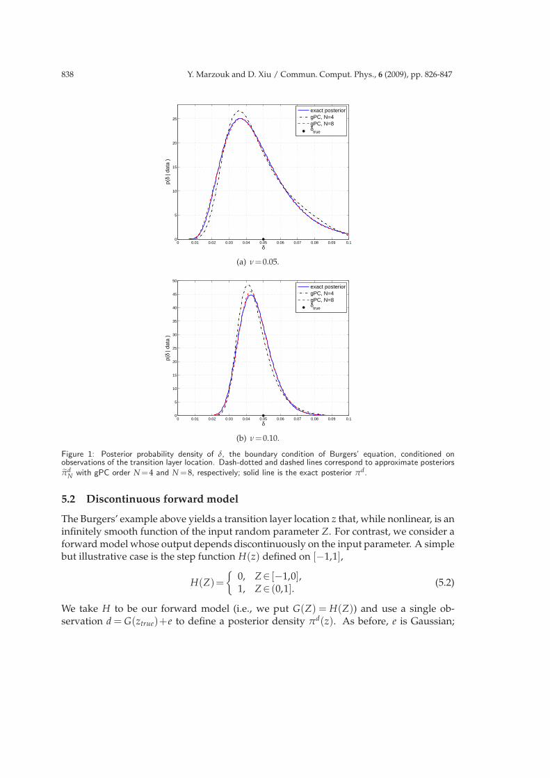
N(z), as described inSection 3.3. For comparison, we also compute the exact posterior density πd(z) using theexact forward model G. Fig. 1 shows the resulting densities at two values of the viscosityν. In both cases, nd = 5 observations were used to estimate δ; these observations areindependent random perturbations to the zex resulting from a “true” value of δ=0.5.

Posterior probability densities in Fig. 1(a)-(b) are non-Gaussian, reflecting the non-linearity of the forward model. A lower value of the viscosity, ν = 0.05, results in abroader posterior density than the larger value ν = 0.10. This phenomenon is a resultof the steady-state solution profile steepening as viscosity decreases. Given a fixed rangeon δ, the resulting distribution of transition layer locations tightens with smaller ν [30];conversely, given a fixed observational error in zex, a wider range of δ values correspondto transitions that fall near the center of the observational distribution—thus spreadingthe posterior probability density over a wider range of δ. In both cases, however, theapproximate posterior densities πd

N(z) approach the exact density with increasing gPCorder N.

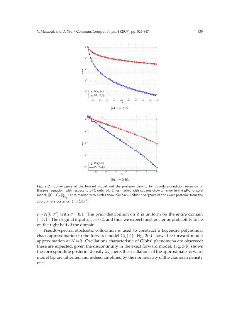
Convergence of the posterior with respect to polynomial order is analyzed morequantitatively in Fig. 2. Again, results are shown for ν = 0.05 and ν = 0.10. We plotthe L2 error in the forward model,

‖G−GN‖2L2

πZ

,

and the Kullback-Leibler divergence of the exact posterior from the approximate poste-rior, D(πd

N‖πd). A large number of collocation points (Q = 800) are employed so thataliasing errors are well-controlled, particularly since results are computed at high order.Since the forward model is smooth, we find the expected exponential convergence of GN

to G at large N. We also observe exponential convergence of the Kullback-Leibler di-vergence at large N. (Dashed lines show log-linear fits at large N.) Moreover, we findthat the posterior Kullback-Leibler divergence converges somewhat faster than the L2 er-ror in the forward model, thus exceeding the (minimal) convergence rate guaranteed byTheorem 4.1.


0 0.01 0.02 0.03 0.04 0.05 0.06 0.07 0.08 0.09 0.10

5

10

15

20

25

δ

p(δ

| dat

a )

exact posteriorgPC, N=4gPC, N=8δ

true

(a) ν=0.05.

0 0.01 0.02 0.03 0.04 0.05 0.06 0.07 0.08 0.09 0.10

5

10

15

20

25

30

35

40

45

50

δ

p(δ

| dat

a )

exact posteriorgPC, N=4gPC, N=8δ

true

(b) ν=0.10.

Figure 1: Posterior probability density of δ, the boundary condition of Burgers’ equation, conditioned onobservations of the transition layer location. Dash-dotted and dashed lines correspond to approximate posteriorsπd

N with gPC order N =4 and N =8, respectively; solid line is the exact posterior πd.

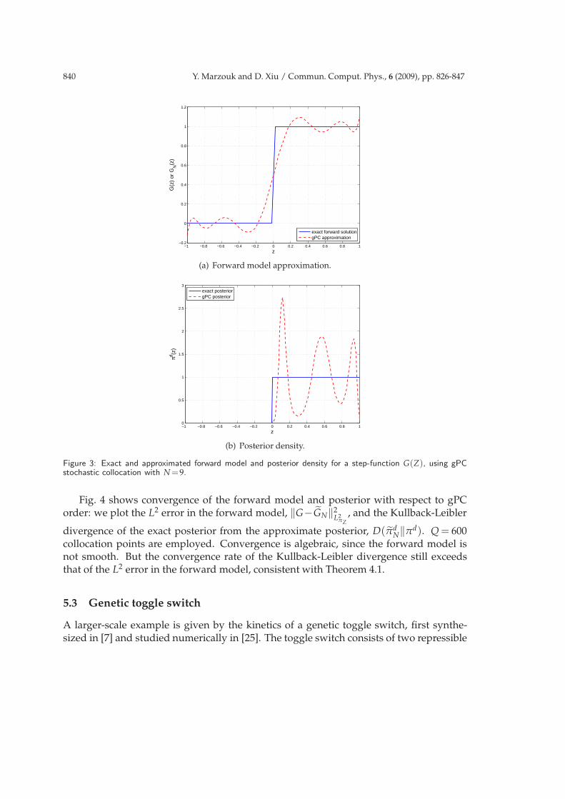
5.2 Discontinuous forward model

The Burgers’ example above yields a transition layer location z that, while nonlinear, is aninfinitely smooth function of the input random parameter Z. For contrast, we consider aforward model whose output depends discontinuously on the input parameter. A simplebut illustrative case is the step function H(z) defined on [−1,1],

H(Z)=

{0, Z∈ [−1,0],1, Z∈ (0,1].

(5.2)

We take H to be our forward model (i.e., we put G(Z) = H(Z)) and use a single ob-servation d = G(ztrue)+e to define a posterior density πd(z). As before, e is Gaussian;


20 40 60 80 100 120 140 160 180 200

10−6

10−5

10−4

10−3

10−2

N

erro

r

D(πN

|| π )

||G − GN

||L

2

(a) ν=0.05.

10 15 20 25 30 35 40

10−6

10−5

10−4

10−3

10−2

N

erro

r

D(πN

|| π )

||G − GN

||L

2

(b) ν=0.10.

Figure 2: Convergence of the forward model and the posterior density for boundary-condition inversion ofBurgers’ equation, with respect to gPC order N. Lines marked with squares show L2 error in the gPC forward

model, ‖G−GN‖2L2

πZ

; lines marked with circles show Kullback-Leibler divergence of the exact posterior from the

approximate posterior, D(πdN‖πd).

e ∼ N(0,σ2) with σ = 0.1. The prior distribution on Z is uniform on the entire domain[−1,1]. The original input ztrue =0.2, and thus we expect most posterior probability to lieon the right half of the domain.

Pseudo-spectral stochastic collocation is used to construct a Legendre polynomialchaos approximation to the forward model GN(Z). Fig. 3(a) shows the forward modelapproximation at N = 9. Oscillations characteristic of Gibbs’ phenomena are observed;these are expected, given the discontinuity in the exact forward model. Fig. 3(b) showsthe corresponding posterior density πd

N ; here, the oscillations of the approximate forward

model GN are inherited and indeed amplified by the nonlinearity of the Gaussian densityof e.


−1 −0.8 −0.6 −0.4 −0.2 0 0.2 0.4 0.6 0.8 1−0.2

0

0.2

0.4

0.6

0.8

1

1.2

z

G(z

) or

GN

(z)

exact forward solutiongPC approximation

(a) Forward model approximation.

−1 −0.8 −0.6 −0.4 −0.2 0 0.2 0.4 0.6 0.8 10

0.5

1

1.5

2

2.5

3

z

πd (z)

exact posteriorgPC posterior

(b) Posterior density.

Figure 3: Exact and approximated forward model and posterior density for a step-function G(Z), using gPCstochastic collocation with N =9.

Fig. 4 shows convergence of the forward model and posterior with respect to gPCorder: we plot the L2 error in the forward model, ‖G−GN‖2

L2πZ

, and the Kullback-Leibler

divergence of the exact posterior from the approximate posterior, D(πdN‖πd). Q = 600

collocation points are employed. Convergence is algebraic, since the forward model isnot smooth. But the convergence rate of the Kullback-Leibler divergence still exceedsthat of the L2 error in the forward model, consistent with Theorem 4.1.

5.3 Genetic toggle switch

A larger-scale example is given by the kinetics of a genetic toggle switch, first synthe-sized in [7] and studied numerically in [25]. The toggle switch consists of two repressible


101

102

10−1

100

N

erro

r

D(π

N || π )

||G − GN

||L

2

Figure 4: Errors in the forward model and posterior density approximations for a step-function G(Z), as afunction of gPC order N.

promotors arranged in a mutually inhibitory network: promoter 1 transcribes a repressorfor promoter 2, while promoter 2 transcribes a repressor for promoter 1. Either repres-sor may be induced by an external chemical or thermal signal. Genetic circuits of thisform have been implemented on E. coli plasmids, and the following differential-algebraic(DAE) model has been proposed [7]:

du

dt=

α1

1+vβ−u,

dv

dt=

α2

1+wγ−v,

w=u

(1+[IPTG]/K)η . (5.3)

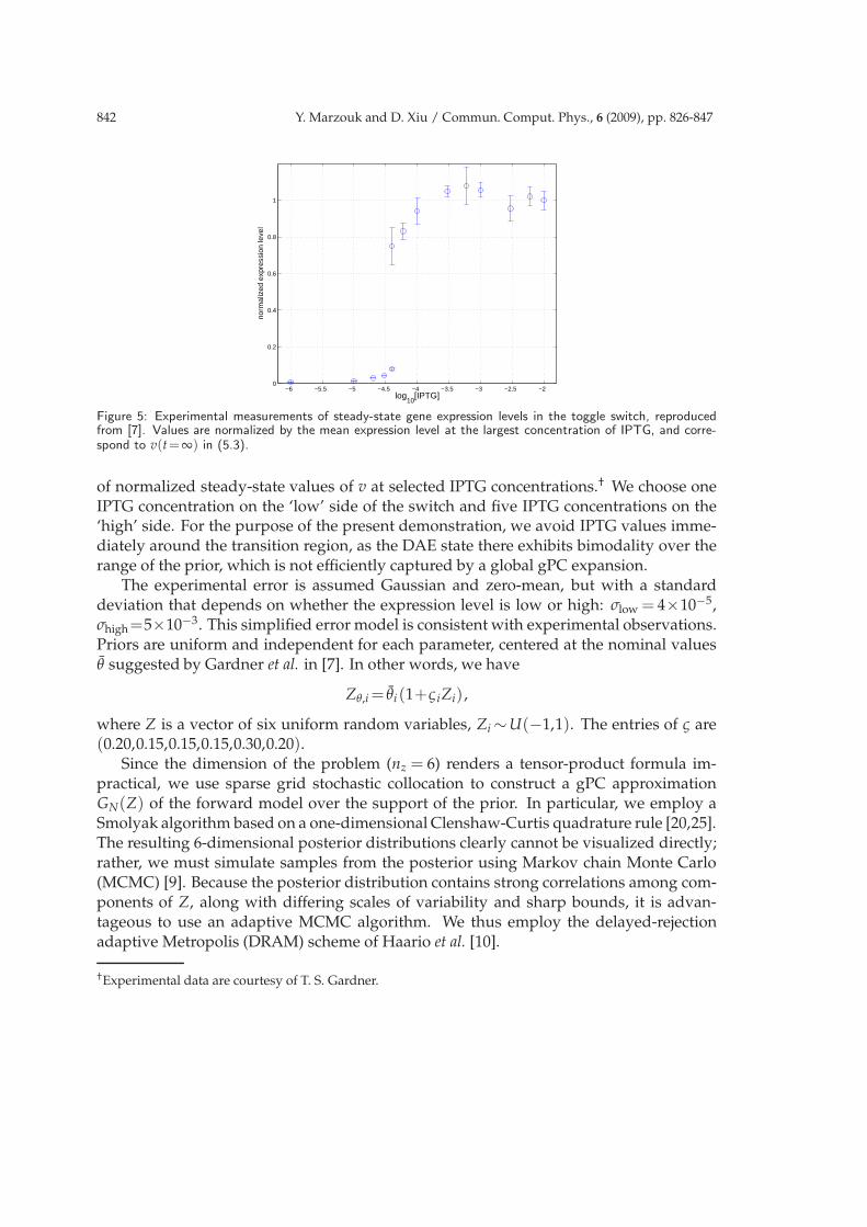
Here u is the concentration of the first repressor and v is the concentration of the secondrepressor; α1 and α2 are the effective rates of synthesis of the repressors; γ and β representcooperativity of repression of promotors 1 and 2, respectively; and [IPTG] is the concen-tration of IPTG, the chemical compound that induces the switch. Parameters K and ηdescribe binding of IPTG with the first repressor. At low values of [IPTG], the switch isin the ‘low’ state, reflected in low values of v; conversely, high values of [IPTG] lead tostrong expression of v. Experimental measurements [7] of steady-state expression levelsv(t=∞) are reproduced in Fig. 5. Observations over a wide range of IPTG concentrationsclearly reveal the two-state behavior of the switch.

Values of the six parameters Zθ =(α1,α2,β,γ,η,K)∈R6 are highly uncertain. Nominal

values were estimated in [7], but here we compute the joint posterior probability densityof these parameters from experimental data. This density will reflect not only nominalvalues (e.g., mean or maximum a posteriori estimates), but variances, correlations, andany other desired measure of uncertainty in the parameter vector Z. Our data consist


−6 −5.5 −5 −4.5 −4 −3.5 −3 −2.5 −20

0.2

0.4

0.6

0.8

1

log10

[IPTG]

norm

aliz

ed e

xpre

ssio

n le

vel

Figure 5: Experimental measurements of steady-state gene expression levels in the toggle switch, reproducedfrom [7]. Values are normalized by the mean expression level at the largest concentration of IPTG, and corre-spond to v(t=∞) in (5.3).

of normalized steady-state values of v at selected IPTG concentrations.† We choose oneIPTG concentration on the ‘low’ side of the switch and five IPTG concentrations on the‘high’ side. For the purpose of the present demonstration, we avoid IPTG values imme-diately around the transition region, as the DAE state there exhibits bimodality over therange of the prior, which is not efficiently captured by a global gPC expansion.

The experimental error is assumed Gaussian and zero-mean, but with a standarddeviation that depends on whether the expression level is low or high: σlow = 4×10−5,σhigh=5×10−3. This simplified error model is consistent with experimental observations.Priors are uniform and independent for each parameter, centered at the nominal valuesθ suggested by Gardner et al. in [7]. In other words, we have

Zθ,i = θi (1+ςiZi) ,

where Z is a vector of six uniform random variables, Zi ∼U(−1,1). The entries of ς are(0.20,0.15,0.15,0.15,0.30,0.20).

Since the dimension of the problem (nz = 6) renders a tensor-product formula im-practical, we use sparse grid stochastic collocation to construct a gPC approximationGN(Z) of the forward model over the support of the prior. In particular, we employ aSmolyak algorithm based on a one-dimensional Clenshaw-Curtis quadrature rule [20,25].The resulting 6-dimensional posterior distributions clearly cannot be visualized directly;rather, we must simulate samples from the posterior using Markov chain Monte Carlo(MCMC) [9]. Because the posterior distribution contains strong correlations among com-ponents of Z, along with differing scales of variability and sharp bounds, it is advan-tageous to use an adaptive MCMC algorithm. We thus employ the delayed-rejectionadaptive Metropolis (DRAM) scheme of Haario et al. [10].

†Experimental data are courtesy of T. S. Gardner.


α1 140 160 1800.005

0.01

0.015

0.02

α2 140 160 180

15.8

15.9

16

15.8 15.9 160

2

4

6

8

10

β 140 160 180

2.2

2.4

2.6

2.8

15.8 15.9 16

2.2

2.4

2.6

2.8

2.2 2.4 2.6 2.80

0.5

1

1.5

2

γ 140 160 1800.85

0.9

0.95

1

1.05

1.1

15.8 15.9 160.85

0.9

0.95

1

1.05

1.1

2.2 2.4 2.6 2.80.85

0.9

0.95

1

1.05

1.1

0.9 1 1.10

5

10

15

η 140 160 180

1.6

1.8

2

2.2

2.4

2.6

15.8 15.9 16

1.6

1.8

2

2.2

2.4

2.6

2.2 2.4 2.6 2.8

1.6

1.8

2

2.2

2.4

2.6

0.9 1 1.1

1.6

1.8

2

2.2

2.4

2.6

1.5 2 2.50

0.5

1

1.5

2

K 140 160 1802.4

2.6

2.8

3

3.2

3.4

x 10−5

15.8 15.9 162.4

2.6

2.8

3

3.2

3.4

x 10−5

2.2 2.4 2.6 2.82.4

2.6

2.8

3

3.2

3.4

x 10−5

0.9 1 1.12.4

2.6

2.8

3

3.2

3.4

x 10−5

1.5 2 2.52.4

2.6

2.8

3

3.2

3.4

x 10−5

2.5 3 3.5x 10

−5

2

4

6

8

10x 104

α1 α2 β γ η K

Figure 6: 1-D and 2-D posterior marginals of parameters in the differential-algebraic model of a genetic toggleswitch, conditioned on experimental data using the full forward model (i.e., with no gPC approximation).

α1 140 160 1800.005

0.01

0.015

0.02

α2 140 160 180

15.8

15.9

16

15.8 15.9 160

2

4

6

8

10

β 140 160 180

2.2

2.4

2.6

2.8

15.8 15.9 16

2.2

2.4

2.6

2.8

2.2 2.4 2.6 2.80

0.5

1

1.5

2

γ 140 160 1800.85

0.9

0.95

1

1.05

1.1

15.8 15.9 160.85

0.9

0.95

1

1.05

1.1

2.2 2.4 2.6 2.80.85

0.9

0.95

1

1.05

1.1

0.9 1 1.10

5

10

15

η 140 160 180

1.6

1.8

2

2.2

2.4

2.6

15.8 15.9 16

1.6

1.8

2

2.2

2.4

2.6

2.2 2.4 2.6 2.8

1.6

1.8

2

2.2

2.4

2.6

0.9 1 1.1

1.6

1.8

2

2.2

2.4

2.6

1.5 2 2.50

0.5

1

1.5

2

K 140 160 1802.4

2.6

2.8

3

3.2

3.4

x 10−5

15.8 15.9 162.4

2.6

2.8

3

3.2

3.4

x 10−5

2.2 2.4 2.6 2.82.4

2.6

2.8

3

3.2

3.4

x 10−5

0.9 1 1.12.4

2.6

2.8

3

3.2

3.4

x 10−5

1.5 2 2.52.4

2.6

2.8

3

3.2

3.4

x 10−5

2.5 3 3.5x 10

−5

2

4

6

8

10x 104

α1 α2 β γ η K

Figure 7: 1-D and 2-D posterior marginals of parameters in the differential-algebraic model of a genetic toggleswitch, conditioned on experimental data using the stochastic collocation Bayesian approach with N =3.


α1 140 160 1800.005

0.01

0.015

0.02

α2 140 160 180

15.8

15.9

16

15.8 15.9 160

2

4

6

8

10

β 140 160 180

2.2

2.4

2.6

2.8

15.8 15.9 16

2.2

2.4

2.6

2.8

2.2 2.4 2.6 2.80

0.5

1

1.5

2

γ 140 160 1800.85

0.9

0.95

1

1.05

1.1

15.8 15.9 160.85

0.9

0.95

1

1.05

1.1

2.2 2.4 2.6 2.80.85

0.9

0.95

1

1.05

1.1

0.9 1 1.10

5

10

15

η 140 160 180

1.6

1.8

2

2.2

2.4

2.6

15.8 15.9 16

1.6

1.8

2

2.2

2.4

2.6

2.2 2.4 2.6 2.8

1.6

1.8

2

2.2

2.4

2.6

0.9 1 1.1

1.6

1.8

2

2.2

2.4

2.6

1.5 2 2.50

0.5

1

1.5

2

K 140 160 1802.4

2.6

2.8

3

3.2

3.4

x 10−5

15.8 15.9 162.4

2.6

2.8

3

3.2

3.4

x 10−5

2.2 2.4 2.6 2.82.4

2.6

2.8

3

3.2

3.4

x 10−5

0.9 1 1.12.4

2.6

2.8

3

3.2

3.4

x 10−5

1.5 2 2.52.4

2.6

2.8

3

3.2

3.4

x 10−5

2.5 3 3.5x 10

−5

2

4

6

8

10x 104

α1 α2 β γ η K

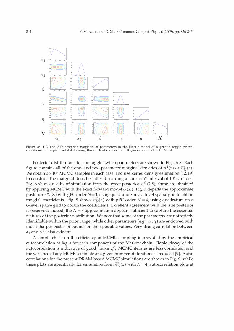
Figure 8: 1-D and 2-D posterior marginals of parameters in the kinetic model of a genetic toggle switch,conditioned on experimental data using the stochastic collocation Bayesian approach with N =4.

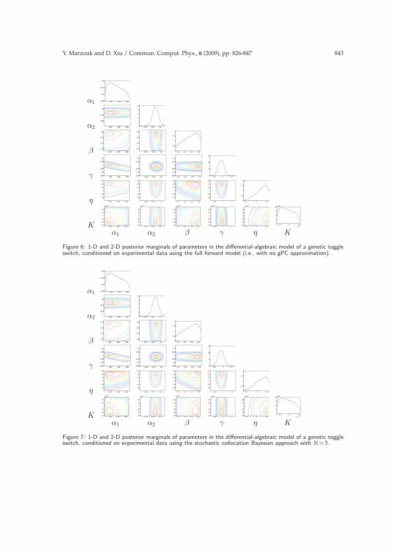
Posterior distributions for the toggle-switch parameters are shown in Figs. 6-8. Eachfigure contains all of the one- and two-parameter marginal densities of πd(z) or πd

N(z).We obtain 3×105 MCMC samples in each case, and use kernel density estimation [12,19]to construct the marginal densities after discarding a “burn-in” interval of 104 samples.Fig. 6 shows results of simulation from the exact posterior πd (2.8); these are obtainedby applying MCMC with the exact forward model G(Z). Fig. 7 depicts the approximateposterior πd

N(Z) with gPC order N=3, using quadrature on a 5-level sparse grid to obtainthe gPC coefficients. Fig. 8 shows πd

N(z) with gPC order N = 4, using quadrature on a6-level sparse grid to obtain the coefficients. Excellent agreement with the true posterioris observed; indeed, the N = 3 approximation appears sufficient to capture the essentialfeatures of the posterior distribution. We note that some of the parameters are not strictlyidentifiable within the prior range, while other parameters (e.g., α2, γ) are endowed withmuch sharper posterior bounds on their possible values. Very strong correlation betweenα1 and γ is also evident.

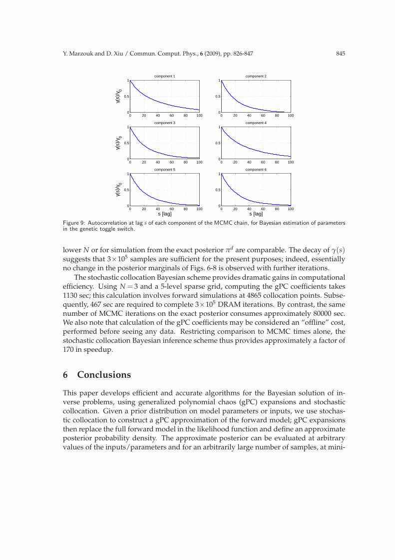
A simple check on the efficiency of MCMC sampling is provided by the empiricalautocorrelation at lag s for each component of the Markov chain. Rapid decay of theautocorrelation is indicative of good “mixing”: MCMC iterates are less correlated, andthe variance of any MCMC estimate at a given number of iterations is reduced [9]. Auto-correlations for the present DRAM-based MCMC simulations are shown in Fig. 9; whilethese plots are specifically for simulation from πd

N(z) with N =4, autocorrelation plots at


0 20 40 60 80 1000

0.5

1component 1

γ(s)

/γ0

0 20 40 60 80 1000

0.5

1component 2

0 20 40 60 80 1000

0.5

1component 3

γ(s)

/γ0

0 20 40 60 80 1000

0.5

1component 4

0 20 40 60 80 1000

0.5

1component 5

s [lag]

γ(s)

/γ0

0 20 40 60 80 1000

0.5

1component 6

s [lag]

Figure 9: Autocorrelation at lag s of each component of the MCMC chain, for Bayesian estimation of parametersin the genetic toggle switch.

lower N or for simulation from the exact posterior πd are comparable. The decay of γ(s)suggests that 3×105 samples are sufficient for the present purposes; indeed, essentiallyno change in the posterior marginals of Figs. 6-8 is observed with further iterations.

The stochastic collocation Bayesian scheme provides dramatic gains in computationalefficiency. Using N = 3 and a 5-level sparse grid, computing the gPC coefficients takes1130 sec; this calculation involves forward simulations at 4865 collocation points. Subse-quently, 467 sec are required to complete 3×105 DRAM iterations. By contrast, the samenumber of MCMC iterations on the exact posterior consumes approximately 80000 sec.We also note that calculation of the gPC coefficients may be considered an “offline” cost,performed before seeing any data. Restricting comparison to MCMC times alone, thestochastic collocation Bayesian inference scheme thus provides approximately a factor of170 in speedup.

6 Conclusions

This paper develops efficient and accurate algorithms for the Bayesian solution of in-verse problems, using generalized polynomial chaos (gPC) expansions and stochasticcollocation. Given a prior distribution on model parameters or inputs, we use stochas-tic collocation to construct a gPC approximation of the forward model; gPC expansionsthen replace the full forward model in the likelihood function and define an approximateposterior probability density. The approximate posterior can be evaluated at arbitraryvalues of the inputs/parameters and for an arbitrarily large number of samples, at mini-


mal computational cost.

We prove the convergence of the approximate posterior to the true posterior, in termsof the Kullback-Leibler divergence (KLD), with increasing gPC order, and obtain an esti-mate of the rate of convergence. In particular, we show that the asymptotic convergencerate of the posterior density is at least the same as the L2 convergence rate of the gPC ex-pansion for the forward solution, and therefore if the gPC representation of the forwardsolution converges exponentially fast, so does the posterior density.

Convergence properties of our algorithm are then demonstrated numerically: firston an infinitely smooth problem involving parameter estimation in the viscous Burgers’equation, and second with a forward model exhibiting discontinuous dependence on itsinput. In both cases, consistency with the predicted convergence rates is obtained. Wethen present an example of kinetic parameter estimation from real experimental data, us-ing stochastic collocation on sparse grids. The latter example shows the utility of sparsegrid constructions for the solution of inverse problems in higher dimensions, and demon-strates that large computational speedups can be obtained with the present stochasticcollocation Bayesian inference scheme.

Acknowledgments

The work of Y. Marzouk is supported in part by the DOE Office of Advanced ScientificComputing Research (ASCR) and by Sandia Corporation (a wholly owned subsidiaryof Lockheed Martin Corporation) as operator of Sandia National Laboratories under USDepartment of Energy contract number DE-AC04-94AL85000. The work of D. Xiu issupported in part by AFOSR FA9550-08-1-0353, NSF CAREER Award DMS-0645035, andthe DOE/NNSA PSAAP center at Purdue (PRISM) under contract number DE-FC52-08NA28617.

References

[1] I. Babuska, F. Nobile, and R. Tempone. A stochastic collocation method for elliptic partialdifferential equations with random input data. SIAM J. Numer. Anal., 45(3):1005–1034, 2007.

[2] I. Babuska, R. Tempone, and G.E. Zouraris. Galerkin finite element approximations ofstochastic elliptic differential equations. SIAM J. Numer. Anal., 42:800–825, 2004.

[3] S. Balakrishnan, A. Roy, M. G. Ierapetritou, G. P. Flach, and P. G. Georgopoulos. Uncertaintyreduction and characterization for complex environmental fate and transport models: anempirical Bayesian framework incorporating the stochastic response surface method. WaterResources Res., 39(12):1350, 2003.

[4] J. A. Christen and C. Fox. MCMC using an approximation. J. Comput. Graph. Stat.,14(4):795–810, 2005.

[5] Y. Efendiev, T. Y. Hou, and W. Luo. Preconditioning Markov chain Monte Carlo simulationsusing coarse-scale models. SIAM J. Sci. Comput., 28:776–803, 2006.

[6] S. N. Evans and P. B. Stark. Inverse problems as statistics. Inverse Problems, 18:R55–R97,2002.


[7] T.S. Gardner, C.R. Cantor, and J.J. Collins. Construction of a genetic toggle switch inEscherichia coli. Nature, 403:339–342, 2000.

[8] R.G. Ghanem and P. Spanos. Stochastic Finite Elements: a Spectral Approach. Springer-Verlag, 1991.

[9] W. R. Gilks, S. Richardson, and D. J. Spiegelhalter. Markov Chain Monte Carlo in Practice.Chapman and Hall, 1996.

[10] H. Haario, M. Laine, A. Mira, and E. Saksman. DRAM: efficient adaptive MCMC. Statisticsand Computing, 16:339–354, 2006.

[11] D. Higdon, H. Lee, and C. Holloman. Markov chain Monte Carlo-based approaches for in-ference in computationally intensive inverse problems. Bayesian Statistics, 7:181–197, 2003.

[12] A. T. Ihler. Kernel density estimation toolbox for MATLAB.http://www.ics.uci.edu/∼ihler/code/kde.html.

[13] J. Kaipio and E. Somersalo. Statistical and Computational Inverse Problems. Springer, 2005.[14] M. C. Kennedy and A. O’Hagan. Bayesian calibration of computer models. J. Royal Statist.

Soc. Series B, 63(3):425–464, 2001.[15] O. Le Maitre, O. Knio, H. Najm, and R. Ghanem. Uncertainty propagation using Wiener-

Haar expansions. J. Comput. Phys., 197:28–57, 2004.[16] Y. M. Marzouk and H. N. Najm. Dimensionality reduction and polynomial chaos accelera-

tion of Bayesian inference in inverse problems. J. Comput. Phys., 228(6):1862–1902, 2009.[17] Y. M. Marzouk, H. N. Najm, and L. A. Rahn. Stochastic spectral methods for efficient

Bayesian solution of inverse problems. J. Comput. Phys., 224(2):560–586, 2007.[18] A. Mohammad-Djafari. Bayesian inference for inverse problems. In Bayesian inference and

Maximum Entropy Methods in Science and Engineering, 21:477–496, 2002.[19] B. W. Silverman. Density Estimation for Statistics and Data Analysis. Chapman & Hall,

1986.[20] S. Smolyak. Quadrature and interpolation formulas for tensor products of certain classes of

functions. Soviet Math. Dokl., 4:240–243, 1963.[21] Ch. Soize and R. Ghanem. Physical systems with random uncertainties: chaos representa-

tions with arbitrary probability measure. SIAM. J. Sci. Comput., 26(2):395–410, 2004.[22] A. Tarantola. Inverse Problem Theory and Methods for Model Parameter Estimation. SIAM,

Philadelphia, 2005.[23] J. Wang and N. Zabaras. Hierarchical Bayesian models for inverse problems in heat conduc-

tion. Inverse Problems, 21:183–206, 2005.[24] J. Wang and N. Zabaras. Using Bayesian statistics in the estimation of heat source in radia-

tion. Int. J. Heat Mass Trans., 48:15–29, 2005.[25] D. Xiu. Efficient collocational approach for parametric uncertainty analysis. Comm. Com-

put. Phys., 2(2):293–309, 2007.[26] D. Xiu. Fast numerical methods for stochastic computations: a review. Comm. Comput.

Phys., 5:242–272, 2009.[27] D. Xiu and J. S. Hesthaven. High-order collocation methods for differential equations with

random inputs. SIAM J. Sci. Comput., 27(3):1118–1139, 2005.[28] D. Xiu and G.E. Karniadakis. The Wiener-Askey polynomial chaos for stochastic differential

equations. SIAM J. Sci. Comput., 24(2):619–644, 2002.[29] D. Xiu and G.E. Karniadakis. Modeling uncertainty in flow simulations via generalized

polynomial chaos. J. Comput. Phys., 187:137–167, 2003.[30] D. Xiu and G.E. Karniadakis. Supersensitivity due to uncertain boundary conditions. Int. J.

Numer. Meth. Engng., 61(12):2114–2138, 2004.

A Stochastic Collocation Approach to Bayesian Inference in Inverse Problems

Documents