Journal of Computational Physics 168, 286–315 (2001) doi:10.1006/jcph.2001.6691, available online at http://www.idealibrary.com on A Staggered Fourth-Order Accurate Explicit Finite Difference Scheme for the Time-Domain Maxwell’s Equations 1 Amir Yefet and Peter G. Petropoulos Department of Mathematical Sciences,New Jersey Institute of Technology, University Heights, Newark, New Jersey 07102 E-mail: [email protected], [email protected] Received November 16, 1999; revised December 18, 2000 We consider a model explicit fourth-order staggered finite-difference method for the hyperbolic Maxwell’s equations. Appropriate fourth-order accurate extrapolation and one-sided difference operators are derived in order to complete the scheme near metal boundaries and dielectric interfaces. An eigenvalue analysis of the overall scheme provides a necessary, but not sufficient, stability condition and indicates long- time stability. Numerical results verify both the stability analysis, and the scheme’s fourth-order convergence rate over complex domains that include dielectric interfaces and perfectly conducting surfaces. For a fixed error level, we find the fourth-order scheme is computationally cheaper in comparison to the Yee scheme by more than an order of magnitude. Some open problems encountered in the application of such high-order schemes are also discussed. c 2001 Academic Press Key Words: Maxwell’s equations, staggered finite-difference schemes, fourth- order schemes, FD-TD scheme. 1. INTRODUCTION Many modern technology applications involve the propagation and scattering of transient electromagnetic signals, e.g., electronic on-chip interconnects, nondestructive testing of concrete structures, and aircraft radar signature analysis. The design and optimization of new systems demands fast and accurate solvers of the time-domain Maxwell equations over complex closed/open domains filled with heterogeneous dielectrics in which metals 1 Supported by AFOSR Grant F49620-99-1-0072 and AFOSR MURI Grant F49620-96-1-0039. 286 0021-9991/01 $35.00 Copyright c 2001 by Academic Press All rights of reproduction in any form reserved.

Welcome message from author
This document is posted to help you gain knowledge. Please leave a comment to let me know what you think about it! Share it to your friends and learn new things together.
Transcript
Journal of Computational Physics168,286–315 (2001)
doi:10.1006/jcph.2001.6691, available online at http://www.idealibrary.com on
A Staggered Fourth-Order Accurate ExplicitFinite Difference Scheme for the Time-Domain
Maxwell’s Equations1
Amir Yefet and Peter G. Petropoulos
Department of Mathematical Sciences, New Jersey Institute of Technology,University Heights, Newark, New Jersey 07102E-mail: [email protected], [email protected]
Received November 16, 1999; revised December 18, 2000
We consider a model explicit fourth-order staggered finite-difference method forthe hyperbolic Maxwell’s equations. Appropriate fourth-order accurate extrapolationand one-sided difference operators are derived in order to complete the scheme nearmetal boundaries and dielectric interfaces. An eigenvalue analysis of the overallscheme provides a necessary, but not sufficient, stability condition and indicates long-time stability. Numerical results verify both the stability analysis, and the scheme’sfourth-order convergence rate over complex domains that include dielectric interfacesand perfectly conducting surfaces. For a fixed error level, we find the fourth-orderscheme is computationally cheaper in comparison to the Yee scheme by more thanan order of magnitude. Some open problems encountered in the application of suchhigh-order schemes are also discussed.c© 2001 Academic Press
Key Words:Maxwell’s equations, staggered finite-difference schemes, fourth-order schemes, FD-TD scheme.
1. INTRODUCTION
Many modern technology applications involve the propagation and scattering of transientelectromagnetic signals, e.g., electronic on-chip interconnects, nondestructive testing ofconcrete structures, and aircraft radar signature analysis. The design and optimization ofnew systems demands fast and accurate solvers of the time-domain Maxwell equationsover complex closed/open domains filled with heterogeneous dielectrics in which metals
1 Supported by AFOSR Grant F49620-99-1-0072 and AFOSR MURI Grant F49620-96-1-0039.
286
0021-9991/01 $35.00Copyright c© 2001 by Academic PressAll rights of reproduction in any form reserved.
FOURTH-ORDER FINITE-DIFFERENCE METHOD 287
are embedded. This is a challenge for numerical modelers as the relevant mathematicalproblem to be solved generally exhibits disparate spatial (e.g., inhomogeneities with bothsmall- and large-scale features) and time (e.g., dispersive media) scales. A mini-review ofthe computational electromagnetics (CEM) state of the art can be found in [1].
Thus far, Yee’s [2–3] finite-difference time-domain (FD-TD) algorithm has provided thebest [4] second-order accurate nondissipative direct solution of the time-domain Maxwellequations on a staggered grid. The numerical error is controlled solely by the mesh size, andthe scheme is particularly easy to implement in the presence of heterogeneous dielectrics andperfectly conducting (PEC) boundaries; it is second-order convergent for planar geometries,where boundaries/interfaces occur on grid points. As all finite difference schemes, the Yeescheme is dispersive and anisotropic, and for large-scale problems, or for problems requiringlong-time integration of Maxwell’s equations, errors from dispersion and anisotropy quicklyaccumulate and become significant unless a fine discretization is used [6]. This leads toprohibitive memory requirements and high computational cost when addressing real-worldproblems.
For some time now, workers in CEM have realized the promise of high-order finite-difference schemes [5–12]. The question of staggered versus unstaggered high-orderschemes has been studied in [13] which showed that, for a given order of accuracy, astaggered scheme is more accurate and efficient than an unstaggered scheme. However, theextended spatial stencil of staggered high-order methods has inhibited their wide accep-tance as it does not allow the easy application of boundary conditions (far-field, impedance,or metal) and the accurate modeling of dielectric interfaces. In this paper we revisit theexplicit(2, 4) scheme of [5], and we use it as a model to address some of the remaining ob-jections to using high-order stencils on a staggered grid. Although it is possible to considera fourth-order time integrator with Fang’s spatial differencing, e.g. [18], we concentrateon the particular (2, 4) scheme herein in order to introduce and study appropriate spatialdifferencing techniques for bounded domains.
We adopt a domain-decomposition point of view and treat dielectric interfaces as bound-ary points between subdomains in which the spatial derivatives are computed to fourth-orderaccuracy; boundary data is imposed as in the Yee scheme. For the model fourth-order spa-tial stencil, we propose a series of numerical boundary conditions, involving one-sideddifferentiation and extrapolation/interpolation, to implement metal boundaries and dielec-tric interfaces when these occur on electric field grid points. Where appropriate, we indicatehow to modify our scheme for the cases where the boundaries, or the dielectric interfaces,occur on magnetic field grid points. Our approach is motivated by [15, 16], which con-sidered the accurate treatment of dielectric interfaces for the second-order Yee scheme (asimilar approach for second-order schemes is developed in [17]). The treatment of metalboundaries herein is different from that used in [6], where the method of images was ap-plicable because of the infinite extent of those boundaries in the numerical tests performedthere. Also, the treatment of dielectric interfaces herein is different from that in [7], wherea simple pointwise specification of dielectric properties was used; we show that such anapproach severely degrades the convergence rate of the scheme. A stability analysis, whichincludes the effects of metal boundaries and dielectric interfaces, is given. We find the nec-essary CFL stability condition derived in [5] also holds when metal boundaries are present,while problems with dielectric interfaces require a slightly smaller CFL number which wedetermine for a given mesh size and dielectric contrast. For the model scheme herein this isnot overly restrictive as one typically chooses a CFL number proportional to the mesh size
288 YEFET AND PETROPOULOS
in order to compute fourth-order accurate results. Numerical experiments show that thesenew numerical boundary conditions preserve the fourth-order accuracy of the scheme whenboundaries/interfaces occur on grid points. We also examine the effect of stair-stepping aboundary not aligned with the grid, and of the presence of geometric singularities.
2. PRELIMINARIES
The Maxwell equations in an isotropic, homogeneous, nondispersive medium are
∂B∂t+∇ × E = 0 (Faraday’s Law),
∂D∂t−∇ × H = 0 (Ampere’s Law),
(1)B = µH,
D = εE.
In the absence of impressed electric charge, the magnetic induction and electric displacementfields satisfy the constraints (Gauss’s law):
∇ · B = 0,(2)
∇ · D = 0.
Scattering obstacles will be modeled by a spatial variation ofε andµ. In free space,ε andµ are constant, equal to their minimum valuesε0, µ0. The speed of light in free space isc = 1√
ε0µ0.
To simplify the notation we will mainly consider two-dimensional problems. In twodimensions, (1) decouples into two independent sets of equations, each representing adistinct polarization. We shall use as our model system of equations those of the transversemagnetic (TM) polarization, where the electric field is a scalar while the magnetic field isa plane vector,
∂Ez
∂t= 1
ε
(∂Hy
∂x− ∂Hx
∂y
),
∂Hx
∂t= − 1
µ
∂Ez
∂y, (3)
∂Hy
∂t= 1
µ
∂Ez
∂x.
Because the fields have noz-dependence, Gauss’ Law is trivially satisfied byD= (0, 0,εEz)
T , while the magnetic fields are constrained to satisfy∇ · (µHx, µHy, 0)T = 0 for alltime. Wave excitation is achieved by imposing appropriate initial and/or boundary con-ditions. We will present numerical examples for dielectrics with (a) piecewise-constantε (µ = µ0), and (b) piecewise-constantµ (ε= ε0). Case (b) can be thought (duality) to rep-resent the transverse electric (TE) polarization problem for a dielectric of piecewise-constantε and fixedµ = µ0. The extension of the work herein to the more general three-dimensionalproblem (1) is straightforward.
FOURTH-ORDER FINITE-DIFFERENCE METHOD 289
3. THE SCHEME IN A HOMOGENEOUS BOUNDED DIELECTRIC
The discretization of (3) with the staggered Yee scheme(O(1t2)-accurate leapfrog timeintegration) is
En+1z,i, j = En
z,i, j +1t
ε1xδx Hn+1/2
y,i, j −1t
ε1yδy Hn+1/2
x,i, j ,
Hn+1/2x,i, j−1/2 = Hn−1/2
x,i, j−1/2−1t
µ1yδyEn
z,i, j−1/2, (4)
Hn+1/2y,i−1/2, j = Hn−1/2
y,i−1/2, j +1t
µ1xδx En
z,i−1/2, j ,
where
δxUi, j = Ui+1/2, j −Ui−1/2, j ,(5)
δyUi, j = Ui, j+1/2−Ui, j+1/2.
Hereafter we shall refer to (4) and (5) as the Yee scheme.In the fourth-order scheme [5] the spatial difference operators (5) are replaced by fourth-
order accurate stencils. For example, to compute a fourth-order accurate approximation ofthe quantity1y ∂U
∂y |(i, j+1/2) we use
δyUi, j = 1
24(Ui, j−1− 27Ui, j + 27Ui, j+1−Ui, j+2). (6)
The Yee scheme can be applied at all nodes in a bounded domain except at the firstand last where boundary conditions are to be imposed. However, the fourth-order stencilrequires numerical boundary conditions at the nodes next to an electric field boundary node.To complete this scheme at the two interior grid points (one electric and one magnetic)immediately next to the first and last electric field grid points of a bounded domain, we usefourth- and third-order accurate one-sided approximations in order to globally approximatethe derivative. No physical boundary conditions are included at this stage. These one-sidedapproximations are
∂U
∂yi,1/2= 1
241y(−22Ui,0+ 17Ui,1+ 9Ui,2− 5Ui,3+Ui,4),
∂U
∂yi,1= 1
241y
(−23Ui,1/2+ 21Ui,3/2+ 3Ui,5/2−Ui,7/2),
(7)∂U
∂yi,N−1= 1
241y
(23Ui,N−1/2− 21Ui,N−3/2− 3Ui,N−5/2+Ui,N−7/2
),
∂U
∂yi,N−1/2= 1
241y(22Ui,N − 17Ui,N−1− 9Ui,N−2+ 5Ui,N−3−Ui,N−4),
for the derivative in they-direction with truncation errors711y4
1920∂5U∂y5 and1y3
24∂4U∂y4 , and simi-
larly for the derivative in thex-direction. Consequently, electric field boundary conditionscan be imposed as in the Yee scheme. Labeling the scheme, which employs (6) in theinterior and (7) near the boundary, a 4− 3− 4− 3− 4 scheme (see [14] for similar nota-tion), we have also tested alternative boundary treatments that result in 4− 4− 4− 4− 4,
290 YEFET AND PETROPOULOS
3− 4− 4− 4− 3, or 3− 3− 4− 3− 3 schemes; such schemes were rejected throughnumerical experimentation as less accurate.
We next define
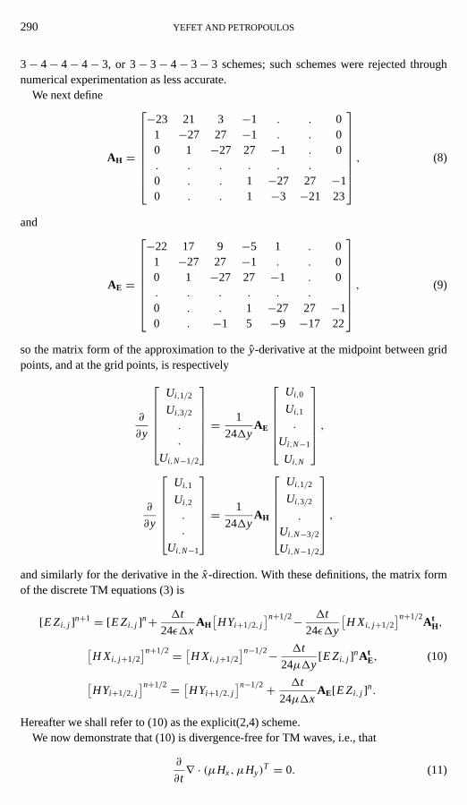
AH =
−23 21 3 −1 . . 01 −27 27 −1 . . 00 1 −27 27 −1 . 0. . . . . .
0 . . 1 −27 27 −10 . . 1 −3 −21 23
, (8)
and
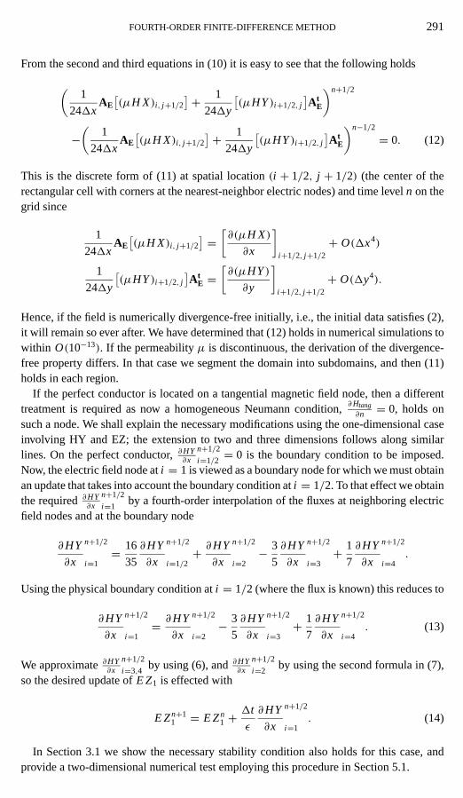
AE =
−22 17 9 −5 1 . 01 −27 27 −1 . . 00 1 −27 27 −1 . 0. . . . . .
0 . . 1 −27 27 −10 . −1 5 −9 −17 22
, (9)
so the matrix form of the approximation to they-derivative at the midpoint between gridpoints, and at the grid points, is respectively
∂
∂y
Ui,1/2
Ui,3/2
.
.
Ui,N−1/2
=1
241yAE
Ui,0
Ui,1
.
Ui,N−1
Ui,N
,
∂
∂y
Ui,1
Ui,2
.
.
Ui,N−1
=1
241yAH
Ui,1/2
Ui,3/2
.
Ui,N−3/2
Ui,N−1/2
,
and similarly for the derivative in thex-direction. With these definitions, the matrix formof the discrete TM equations (3) is
[E Zi, j ]n+1 = [E Zi, j ]
n+ 1t
24ε1xAH[HYi+1/2, j
]n+1/2− 1t
24ε1y
[H Xi, j+1/2
]n+1/2At
H,[H Xi, j+1/2
]n+1/2 = [H Xi, j+1/2]n−1/2− 1t
24µ1y[E Zi, j ]
nAtE, (10)
[HYi+1/2, j
]n+1/2 = [HYi+1/2, j]n−1/2+ 1t
24µ1xAE[E Zi, j ]
n.
Hereafter we shall refer to (10) as the explicit(2,4) scheme.We now demonstrate that (10) is divergence-free for TM waves, i.e., that
∂
∂t∇ · (µHx, µHy)
T = 0. (11)
FOURTH-ORDER FINITE-DIFFERENCE METHOD 291
From the second and third equations in (10) it is easy to see that the following holds
(1
241xAE[(µH X)i, j+1/2
]+ 1
241y
[(µHY)i+1/2, j
]At
E
)n+1/2
−(
1
241xAE[(µH X)i, j+1/2
]+ 1
241y
[(µHY)i+1/2, j
]At
E
)n−1/2
= 0. (12)
This is the discrete form of (11) at spatial location(i + 1/2, j + 1/2) (the center of therectangular cell with corners at the nearest-neighbor electric nodes) and time leveln on thegrid since
1
241xAE[(µH X)i, j+1/2
] = [∂(µH X)
∂x
]i+1/2, j+1/2
+ O(1x4)
1
241y
[(µHY)i+1/2, j
]At
E =[∂(µHY)
∂y
]i+1/2, j+1/2
+ O(1y4).
Hence, if the field is numerically divergence-free initially, i.e., the initial data satisfies (2),it will remain so ever after. We have determined that (12) holds in numerical simulations towithin O(10−13). If the permeabilityµ is discontinuous, the derivation of the divergence-free property differs. In that case we segment the domain into subdomains, and then (11)holds in each region.
If the perfect conductor is located on a tangential magnetic field node, then a differenttreatment is required as now a homogeneous Neumann condition,∂Htang
∂n = 0, holds onsuch a node. We shall explain the necessary modifications using the one-dimensional caseinvolving HY and EZ; the extension to two and three dimensions follows along similarlines. On the perfect conductor,∂HY
∂xn+1/2
i=1/2= 0 is the boundary condition to be imposed.
Now, the electric field node ati = 1 is viewed as a boundary node for which we must obtainan update that takes into account the boundary condition ati = 1/2. To that effect we obtainthe required∂HY
∂xn+1/2
i=1by a fourth-order interpolation of the fluxes at neighboring electric
field nodes and at the boundary node
∂HY
∂x
n+1/2
i=1= 16
35
∂HY
∂x
n+1/2
i=1/2+ ∂HY
∂x
n+1/2
i=2− 3
5
∂HY
∂x
n+1/2
i=3+ 1
7
∂HY
∂x
n+1/2
i=4.
Using the physical boundary condition ati = 1/2 (where the flux is known) this reduces to
∂HY
∂x
n+1/2
i=1= ∂HY
∂x
n+1/2
i=2− 3
5
∂HY
∂x
n+1/2
i=3+ 1
7
∂HY
∂x
n+1/2
i=4. (13)
We approximate∂HY∂x
n+1/2
i=3,4by using (6), and∂HY
∂xn+1/2
i=2by using the second formula in (7),
so the desired update ofE Z1 is effected with
E Zn+11 = E Zn
1 +1t
ε
∂HY
∂x
n+1/2
i=1. (14)
In Section 3.1 we show the necessary stability condition also holds for this case, andprovide a two-dimensional numerical test employing this procedure in Section 5.1.
292 YEFET AND PETROPOULOS
3.1. Stability
A standard Von Neumann analysis of (4) and (5) on an unbounded uniform Cartesiangrid with mesh sizeh results in the well-known CFL stability condition
1t√min{ε · µ} ≤
h√d,
whered is the number of spatial dimensions [3]. The application of boundary conditions onelectric field grid points does not alter the stability condition. When dielectrics are present,one first determines the maximumh for accuracy by using the max{ε · µ} over the domainof interest and the maximum frequency to be resolved with a preset number of pointsper wavelength; the stability condition then sets the maximum allowed time step for thatparticularh.
A similar analysis for (4) and (6) on an unbounded uniform Cartesian grid with meshsizeh results in the CFL condition
1t√min{ε · µ} ≤ 2
h
ρ∞[5],
whereρ∞ is the spectral radius of the matrices used to compute spatial derivatives; forthe differentiation matrix scaled byh, it is ρ∞ = 7
3
√d. In this paper we consider (10) for
d = 1, 2, 3, and the following eigenvalue analysis verifies that the same necessary conditionholds for stability over bounded domains; we do not prove herein that this condition is alsosufficient for stability.
First, we analyze the stability of thed = 1 semi-discrete versions of (10)(1t → 0 for afixed h 6= 0) on a bounded domain in order to determine whether the inclusion of the one-sided differencing operators and the imposition of boundary conditions result in a stablescheme. We will do so by neglecting the [H X] grid function, settingh = 1x, ε = µ = 1,and considering the system
dudt= 1
hM · u. (15)
The vectoru = {E Z0, E Z1, . . . , E ZN−1, E ZN, HY1/2, HY3/2, . . . , HYN−3/2, HYN−1/2}is the solution on the grid, andM is the matrix composed of the difference operatorsrepresented by (8) and (9). We will consider the case in whichM enforces homogeneousDirichlet boundary conditionsE Z0 = E ZN = 0 at the first and last (boundary) nodes ofthe grid. Assumingu = eλt u, whereλ are the eigenvalues ofM , andu is a complex-valuedconstant vector, the spectral radius ofM , providedR{λ} = 0, will be ρM = max|={λ}|,and the semi-discrete scheme will be stable. The fully discrete scheme, using staggeredLeapfrog time integration and including the caseε, µ 6= 1, will be stable when
1t√min{ε · µ} ≤ 2
h
ρM. (16)
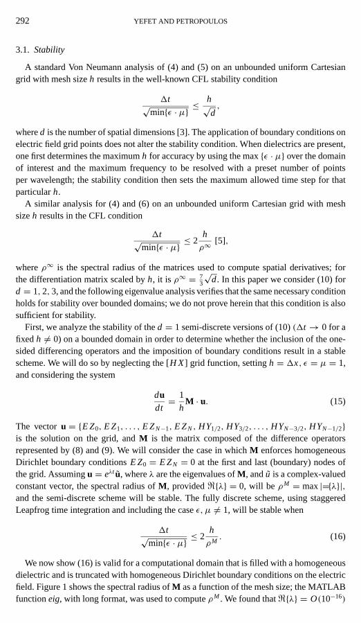
We now show (16) is valid for a computational domain that is filled with a homogeneousdielectric and is truncated with homogeneous Dirichlet boundary conditions on the electricfield. Figure 1 shows the spectral radius ofM as a function of the mesh size; the MATLABfunctioneig, with long format, was used to computeρM . We found thatR{λ} = O(10−16)
FOURTH-ORDER FINITE-DIFFERENCE METHOD 293
FIG. 1. The spectral radiusρM as a function of mesh size for Dirichlet boundary conditions.
for all h. As h→ 0, ρM → ρ∞ from below, i.e., the explicit(2, 4) on a bounded domain isstable for the same CFL number as in an unbounded domain.
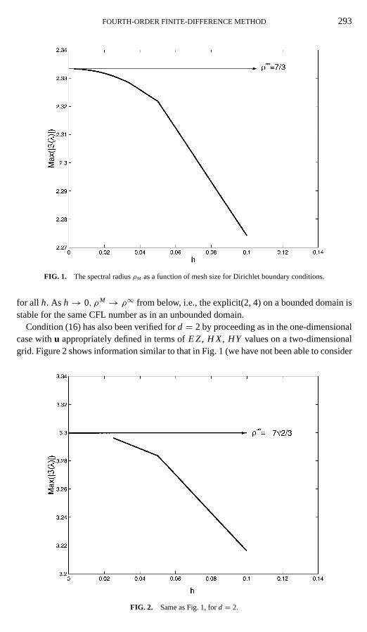
Condition (16) has also been verified ford = 2 by proceeding as in the one-dimensionalcase withu appropriately defined in terms ofE Z, H X, HY values on a two-dimensionalgrid. Figure 2 shows information similar to that in Fig. 1 (we have not been able to consider
FIG. 2. Same as Fig. 1, ford = 2.
294 YEFET AND PETROPOULOS
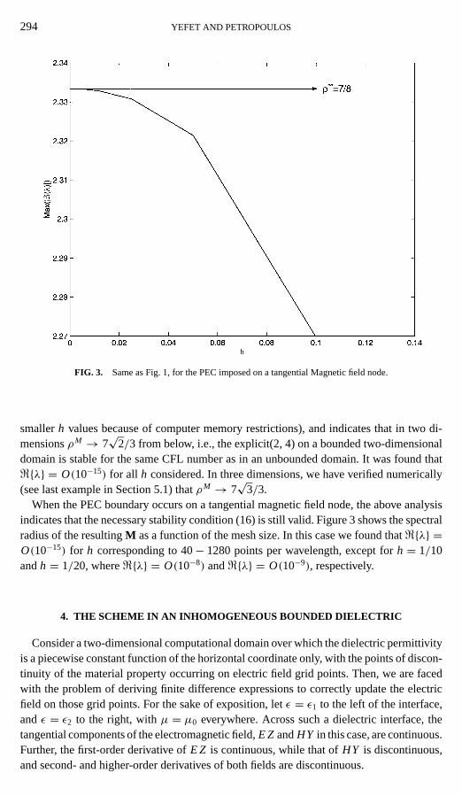
FIG. 3. Same as Fig. 1, for the PEC imposed on a tangential Magnetic field node.
smallerh values because of computer memory restrictions), and indicates that in two di-mensionsρM → 7
√2/3 from below, i.e., the explicit(2, 4) on a bounded two-dimensional
domain is stable for the same CFL number as in an unbounded domain. It was found thatR{λ} = O(10−15) for all h considered. In three dimensions, we have verified numerically(see last example in Section 5.1) thatρM → 7
√3/3.
When the PEC boundary occurs on a tangential magnetic field node, the above analysisindicates that the necessary stability condition (16) is still valid. Figure 3 shows the spectralradius of the resultingM as a function of the mesh size. In this case we found thatR{λ} =O(10−15) for h corresponding to 40− 1280 points per wavelength, except forh = 1/10andh = 1/20, whereR{λ} = O(10−8) andR{λ} = O(10−9), respectively.
4. THE SCHEME IN AN INHOMOGENEOUS BOUNDED DIELECTRIC
Consider a two-dimensional computational domain over which the dielectric permittivityis a piecewise constant function of the horizontal coordinate only, with the points of discon-tinuity of the material property occurring on electric field grid points. Then, we are facedwith the problem of deriving finite difference expressions to correctly update the electricfield on those grid points. For the sake of exposition, letε = ε1 to the left of the interface,andε = ε2 to the right, withµ = µ0 everywhere. Across such a dielectric interface, thetangential components of the electromagnetic field,E Z andHY in this case, are continuous.Further, the first-order derivative ofE Z is continuous, while that ofHY is discontinuous,and second- and higher-order derivatives of both fields are discontinuous.
FOURTH-ORDER FINITE-DIFFERENCE METHOD 295
To implement the Yee scheme on a dielectric interface we setεinterface= ε1+ε22 . This can
be shown to be the appropriate material property for the grid point of discontinuity, asa local truncation error analysis indicates first-order accuracy in the mesh size; then, theglobal second-order convergence rate of the scheme is not affected as it is also confirmedby the numerical results. The implementation of discontinuous dielectric properties in theexplicit(2, 4) via a fourth-order explicit interpolation of the dielectric permittivity on electricfield nodes results, as our numerical experiments (Section 5.2) show, in a loss of two orders inthe convergence rate of the explicit(2, 4). The same convergence rate reduction is obtainedwhen the method outlined for the Yee scheme is employed to model an interface in theexplicit(2, 4).
An innovative approach to handle piecewise-constant dielectric properties for the Yeescheme, when the discontinuities occur between grid points, is presented in [15, 16]. Herein,we extend this approach to include such dielectric properties in the explicit(2, 4) schemeas long as the discontinuities occur on electric field grid points. The numerical experi-ments in Section 5 confirm a global fourth-order convergence rate for the scheme presentedbelow.
We present our approach for the problem of a vertical dielectric slab placed in a domainbounded on all sides by a metal. We divide the computational domain into three subdomains;two contain air, and the third one contains the lossless dielectric. Inside each subdomain,the difference equations (10) are applied to update the solution. The Dirichlet conditionon the electric field is used to complete the scheme near the metal boundaries (see Section 3).The dielectric interface is also treated as a boundary point for the scheme (10) in the adjacentsubdomains. Suppose those dielectric interfaces are located ati = I1 andi = I2, andε = ε2
for I1 < i < I2 while ε = ε1 for i > I2 andi < I1. We need to derive difference equationsto update the electric field on these boundaries (the dielectric interfaces). We assign eachinterface node to belong to one of the two abutting subdomains, and require that we donot difference across the jump in the material properties. In this particular case, we takei = I1, I2 to be the boundary nodes of the subdomain that is filled with the dielectricε = ε2.To that effect, we first approximateHY (which is continuous across the interface) ati = I1
andi = I2 by using the following fifth-order extrapolation with data from the subdomainthat does not contain the interface node:
HYn+1/2I1, j = 315
128HYn+1/2
I1−1/2, j −105
32HYn+1/2
I1−3/2, j +189
64HYn+1/2
I1−5/2, j
− 45
32HYn+1/2
I1−7/2, j +35
128HYn+1/2
I1−9/2, j
HYn+1/2I2, j = 315
128HYn+1/2
I2+1/2, j −105
32HYn+1/2
I2+3/2, j +189
64HYn+1/2
I2+5/2, j
− 45
32HYn+1/2
I2+7/2, j +35
128HYn+1/2
I2+9/2, j .
(17)
OnceHY is approximated on the interface (i.e., on the boundary node), we approximateits x-derivative at that location using data from the subdomain that contains the interface as
296 YEFET AND PETROPOULOS
a boundary (i.e., we do not difference across interfaces) as follows:
1x∂
∂xHYn+1/2
I1, j = −1126
315HYn+1/2
I1, j + 315
64HYn+1/2
I1+1/2−35
16HYn+1/2
I1+3/2, j
+ 189
160HYn+1/2
I1+5/2, j −45
112HYn+1/2
I1+7/2, j +35
576HYn+1/2
I1+9/2, j
1x∂
∂xHYn+1/2
I2, j = 1126
315HYn+1/2
I2, j − 315
64HYn+1/2
I2−1/2+35
16HYn+1/2
I2−3/2, j
− 189
160HYn+1/2
I2−5/2, j +45
112HYn+1/2
I2−7/2, j −35
576HYn+1/2
I2−9/2, j .
(18)
Once ∂∂x HYn+1/2
I1, j and ∂∂x HYn+1/2
I2, j are calculated, we update the electric field on the interfacesby evaluatingE Zn+1
I1, j andE Zn+1I2, j in the following way, e.g., ati = I1:
E Zn+1I1, j = E Zn
I1, j −1t
ε2241y
(H Xn+1/2
I1, j−3/2− 27H Xn+1/2I1, j−1/2+ 27H Xn+1/2
I1, j+1/2− H Xn+1/2I1, j+3/2
)+ 1t
ε2
∂
∂xHYn+1/2
I1, j . (19)
Similarly, ati = I2 to updateE Zn+1I2, j .
For a given dielectric contrast we found that differencing inside the subdomain (whileextrapolating to the interface the field variable to be differenced using data from outside thesubdomain) with the smaller dielectric constant results in a slight improvement of the error.Also, we observed that this improvement is lost for large contrast, and therefore concludedthat it does not, in general, matter which subdomain we choose inside which do difference.This is because higher contrasts imply a larger loss of smoothness across the dielectricinterface and a consequent increase of the local error.
If the dielectric interface is located ati = I1+ 1/2, where a tangential magnetic field iscollocated, the treatment differs slightly from that given above. Now, EZ and HY exchangeroles. We first extrapolate EZ to the interface (using data outside the subdomain that containsthe interface)
E ZnI1+1/2, j =
315
128E Zn
I1, j −105
32E Zn
I1−1, j +189
64E Zn
I1−2, j
− 45
32E Zn
I1−3, j +35
128E Zn
I1−4, j ,
and then approximate thex derivative of EZ at that location (using data from the subdomainthat contains the interface as a boundary)
1x∂
∂xE Zn
I1+1/2, j = −1126
315E Zn
I1+1/2, j +315
64E Zn
I1+1, j −35
16E Zn
I1+2, j
+ 189
160E Zn
I1+3, j −45
112E Zn
I1+4, j +35
576E Zn
I1+5, j .
Finally, we update the magnetic field ati = I1+ 1/2 with
HYn+1/2I1+1/2, j = HYn−1/2
I1+1/2, j +1t
µ
∂
∂xE Zn
I1+1/2, j .
We do not pursue this case any further in the present paper.
FOURTH-ORDER FINITE-DIFFERENCE METHOD 297
4.1. Stability
A stability analysis is now given for the semi-discrete version of (10)(1t → 0 for a fixedh 6= 0). Again, we consider a one-dimensional(d = 1) bounded domain separated in twohalves by a dielectric interface at the electric field grid pointI = Iint. We neglect the [H X]grid function, seth = 1x, ε = µ = 1 for grid pointsi < Iint andε = ε2 for grid pointsi ≥ I int, and consider the system
dudt= 1
hMd · u, (20)
whereu = {E Z0, E Z1, . . . , E ZN−1, E ZN, HY1/2, HY3/2, . . . , HYN−3/2, HYN−1/2} is thesolution vector on the grid, andMd is the matrix composed of the difference opera-tors represented by (8), (9), and (17)–(19). Again, we consider the case in whichMenforces homogeneous Dirichlet boundary conditionsE Z0 = E ZN = 0 at the first andlast (boundary) nodes of the grid. As in Section 3.2, if the eigenvaluesλ of Md aresuch thatR{λ} = 0, the spectral radius ofMd will be ρMd = max|={λ}|, and then thesemi-discrete scheme will be stable. Consequently, a necessary (again, not sufficient) sta-bility condition for the fully discrete scheme (including the caseε, µ 6= 1) is (16) withρM = ρMd .
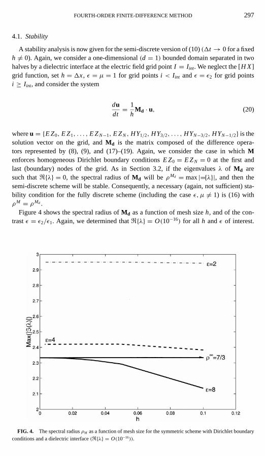
Figure 4 shows the spectral radius ofMd as a function of mesh sizeh, and of the con-trastε = ε2/ε1. Again, we determined thatR{λ} = O(10−16) for all h andε of interest.
FIG. 4. The spectral radiusρM as a function of mesh size for the symmetric scheme with Dirichlet boundaryconditions and a dielectric interface(R{λ} = O(10−16)).
298 YEFET AND PETROPOULOS
However, as the figure shows, the maximum allowed CFL number is now smaller thanthat obtained in Section 3.2 because the value ofρMd , whenh→ 0, depends onε andcan be greater thanρ∞ for someε. We note that for a givenε, ρMd again approachesa limit from below ash→ 0. Therefore, in this case, we can only say that the inter-face treatment is stable and, in general, requires a slight reduction of the maximum al-lowed time step (for a givenh). This is not restrictive for the model scheme consideredherein as one would run it with a small CFL number in order to obtain fourth-orderaccurate results. The stability condition for dielectrics has been verified numerically ford = 1, 2.
The decision to approximate∂∂x HYn+1/2
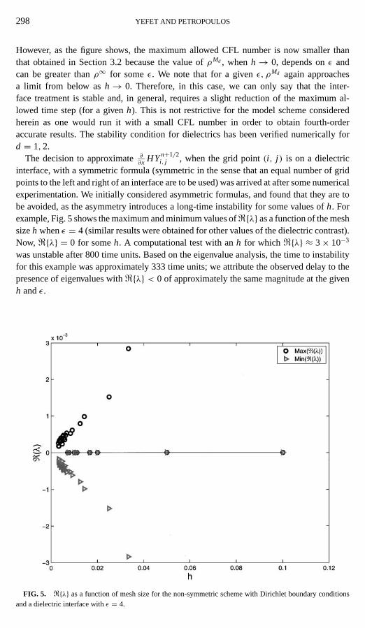
i, j , when the grid point(i, j ) is on a dielectricinterface, with a symmetric formula (symmetric in the sense that an equal number of gridpoints to the left and right of an interface are to be used) was arrived at after some numericalexperimentation. We initially considered asymmetric formulas, and found that they are tobe avoided, as the asymmetry introduces a long-time instability for some values ofh. Forexample, Fig. 5 shows the maximum and minimum values ofR{λ} as a function of the meshsizeh whenε = 4 (similar results were obtained for other values of the dielectric contrast).Now, R{λ} = 0 for someh. A computational test with anh for which R{λ} ≈ 3× 10⁻³
was unstable after 800 time units. Based on the eigenvalue analysis, the time to instabilityfor this example was approximately 333 time units; we attribute the observed delay to thepresence of eigenvalues withR{λ} < 0 of approximately the same magnitude at the givenh andε.
FIG. 5. R{λ} as a function of mesh size for the non-symmetric scheme with Dirichlet boundary conditionsand a dielectric interface withε = 4.
FOURTH-ORDER FINITE-DIFFERENCE METHOD 299
5. COMPUTATIONAL RESULTS
This section provides numerical tests of the boundary/interface treatment for theexplicit(2, 4). At the same time we compare the results to those obtained with the Yeescheme, and, when available, to those obtained with the compact-implicit Ty(2, 4) scheme[10]. All three schemes are advanced in time by theO(1t2)-accurate staggered leapfrogmethod, and a uniform grid spacing is employed. For all computations (except one, whichmodels the transverse electric case) we chooseµ = 1 everywhere, andε = 1 for grid pointsin empty space, whileε > 1 for grid points inside a dielectric medium. In all our tests, metalboundaries and dielectric interfaces occur on electric field grid points. When presented, theerror is measured against the exact solution forEz in the L2 norm over space (except inexample two in Section 5.3, where the error is measured in theL∞ norm over a planecurve). We also provide tables of the error in theL∞ norm over a fixed time interval forthe purpose of deducing convergence rates. For the examples posed in an open domain,we restrict the time interval over which we measure the error so that our computed resultsare not contaminated by reflections from the far-field boundary treatment. All examples inSections 5.1–5.3 were coded in MATLAB.
5.1. Closed Homogeneous Domains
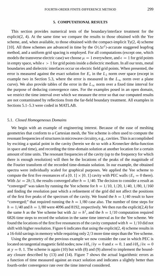
We begin with an example of engineering interest. Because of the ease of meshinggeometries that conform to a Cartesian mesh, the Yee scheme is often used to compute theresonant frequencies of structures in microwave circuitry, e.g., cavities. This is accomplishedby exciting a spatial point in the cavity (herein we do so with a Kronecker delta-functionin space and time), and recording the time-domain solution at another location for a certainamount of time units. The resonant frequencies of the cavity (up to the frequency for whichthere is enough resolution) will then be the locations of the peaks of the magnitude ofthe Fourier transform of the recorded time-domain solution. In our example, the obtainedspectra were individually scaled for graphical purposes. We applied the Yee scheme tocompute the first five resonances of a [0, 1]× [0, 1] cavity with PEC walls(Ez = 0 there).With1t = 2h/3, the results converged afterh = 1/40. The decision to consider a result as“converged” was taken by running the Yee scheme forh = 1/10, 1/20, 1/40, 1/80, 1/160and finding the resolution past which a refinement of the grid did not affect the positionsof the first five peaks of the spectrum of the cavity. We found theh = 1/40 result to have“converged;” that required running theh = 1/80 case also. The number of time steps forh = 1/40 andh = 1/80 were 4096 and 8192, respectively. We then run the explicit(2,4) forthe sameh as the Yee scheme but with1t = h2, and theh = 1/10 computation required6826 time steps to record the solution in the same time interval as for the Yee scheme. Wefound the locations of the first five resonances of the cavity computed withh = 1/10 did notshift with higher resolution. Figure 6 indicates that using the explicit(2, 4) scheme results ina 16-fold savings in memory while requiring only 2/3 more time steps than the Yee scheme.
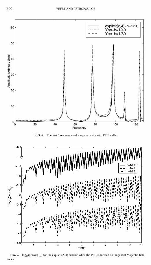
Using the geometry of the previous example we now consider the case in which PEC islocated on tangential magnetic field nodes; now∂Hx/∂y = 0 andx = 0, 1 and∂Hy/∂x = 0at y = 0, 1. The scheme is again (10) but with (8) and (9) altered to implement the bound-ary closure described by (13) and (14). Figure 7 shows the actual logarithmic errors asa function of time measured against an exact solution and indicates a slightly better thanfourth-order convergence rate over the time interval considered.
300 YEFET AND PETROPOULOS
FIG. 6. The first 5 resonances of a square cavity with PEC walls.
FIG. 7. log10(‖error‖L2) for the explicit(2, 4) scheme when the PEC is located on tangential Magentic fieldnodes.
FOURTH-ORDER FINITE-DIFFERENCE METHOD 301
We next consider single-mode propagation in a rectangular cross-section waveguide withperfectly conducting walls. We prescribe initial and boundary conditions,
Ez(x, y, 0) = sin(3πx) sin(4πy),
Hy
(x, y,
1t
2
)= −3
5sin
(3πx − 5π1t
2
)sin(4πy),
Hx
(x, y,
1t
2
)= −4
5cos
(3πx − 5π1t
2
)sin(4πy),
Ez(0, y, t) = −sin(5π t) sin(4πy),
Ez(1, y, t) = sin(3π − 5π t) sin(4πy),
Ez(x, 0, t) = 0,
Ez(x, 1, t) = 0,
so the exact solution is
Ez(x, y, t) = sin(3πx − 5π t) sin(4πy).
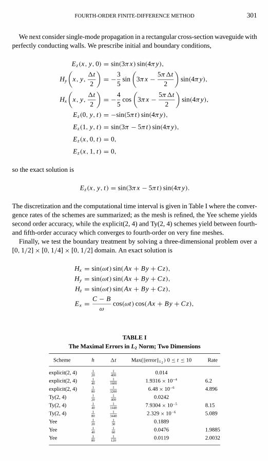
The discretization and the computational time interval is given in Table I where the conver-gence rates of the schemes are summarized; as the mesh is refined, the Yee scheme yieldssecond order accuracy, while the explicit(2, 4) and Ty(2, 4) schemes yield between fourth-and fifth-order accuracy which converges to fourth-order on very fine meshes.
Finally, we test the boundary treatment by solving a three-dimensional problem over a[0, 1/2]× [0, 1/4]× [0, 1/2] domain. An exact solution is
Hx = sin(ωt) sin(Ax+ By+ Cz),
Hy = sin(ωt) sin(Ax+ By+ Cz),
Hz = sin(ωt) sin(Ax+ By+ Cz),
Ex = C − B
ωcos(ωt) cos(Ax+ By+ Cz),
TABLE I
The Maximal Errors in L2 Norm; Two Dimensions
Scheme h 1t Max(‖error‖L2) 0≤ t ≤ 10 Rate
explicit(2, 4) 120
1400
0.014
explicit(2, 4) 140
11600
1.9316× 10⁻⁴ 6.2
explicit(2, 4) 180
13200
6.48× 10⁻⁶ 4.896
Ty(2, 4) 120
1400
0.0242
Ty(2, 4) 140
11440
7.9304× 10⁻⁵ 8.15
Ty(2, 4) 180
13440
2.329× 10⁻⁶ 5.089
Yee 120
130
0.1889
Yee 140
160
0.0476 1.9885
Yee 180
1120
0.0119 2.0032
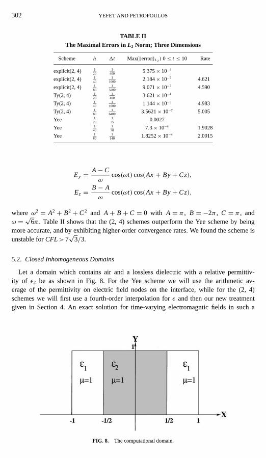
302 YEFET AND PETROPOULOS
TABLE II
The Maximal Errors in L2 Norm; Three Dimensions
Scheme h 1t Max(‖error‖L2) 0≤ t ≤ 10 Rate
explicit(2, 4) 120
1400
5.375× 10⁻⁴
explicit(2, 4) 140
11600
2.184× 10⁻⁵ 4.621
explicit(2, 4) 180
13200
9.071× 10⁻⁷ 4.590
Ty(2, 4) 120
1400
3.621× 10⁻⁴
Ty(2, 4) 140
11600
1.144× 10⁻⁵ 4.983
Ty(2, 4) 180
16400
3.5621× 10⁻⁷ 5.005
Yee 120
135
0.0027
Yee 140
170
7.3× 10⁻⁴ 1.9028
Yee 180
1140
1.8252× 10⁻⁴ 2.0015
Ey = A− C
ωcos(ωt) cos(Ax+ By+ Cz),
Ez = B− A
ωcos(ωt) cos(Ax+ By+ Cz),
whereω2 = A2+ B2+ C2 and A+ B+ C = 0 with A = π , B = −2π , C = π , andω = √6π . Table II shows that the (2, 4) schemes outperform the Yee scheme by beingmore accurate, and by exhibiting higher-order convergence rates. We found the scheme isunstable forCFL> 7
√3/3.
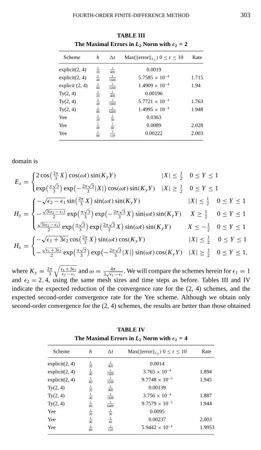
5.2. Closed Inhomogeneous Domains
Let a domain which contains air and a lossless dielectric with a relative permittiv-ity of ε2 be as shown in Fig. 8. For the Yee scheme we will use the arithmetic av-erage of the permittivity on electric field nodes on the interface, while for the (2, 4)schemes we will first use a fourth-order interpolation forε and then our new treatmentgiven in Section 4. An exact solution for time-varying electromagntic fields in such a
FIG. 8. The computational domain.
FOURTH-ORDER FINITE-DIFFERENCE METHOD 303
TABLE III
The Maximal Errors in L2 Norm with ε2 = 2
Scheme h 1t Max(‖error‖L2) 0≤ t ≤ 10 Rate
explicit(2, 4) 120
1400
0.0019
explicit(2, 4) 140
11600
5.7585× 10⁻⁴ 1.715
explicit (2, 4) 180
13200
1.4909× 10⁻⁴ 1.94
Ty(2, 4) 120
1400
0.00196
Ty(2, 4) 140
11600
5.7721× 10⁻⁴ 1.763
Ty(2, 4) 180
16400
1.4995× 10⁻⁴ 1.948
Yee 120
130
0.0363
Yee 140
160
0.0089 2.028
Yee 180
1120
0.00222 2.003
domain is
Ez ={
2 cos(
2π3 X)
cos(ωt) sin(KyY) |X| ≤ 12 0≤ Y ≤ 1
exp(π√
33
)exp(− 2π
√3
3 |X|)
cos(ωt) sin(KyY) |X| ≥ 12 0≤ Y ≤ 1
Hy =
−√ε2− ε1 sin
(2π3 X)
sin(ωt) sin(KyY) |X| ≤ 12 0≤ Y ≤ 1
−√
3(ε2− ε1)
2 exp(π√
33
)exp(− 2π
√3
3 X)
sin(ωt) sin(KyY) X ≥ 12 0≤ Y ≤ 1
√3(ε2− ε1)
2 exp(π√
33
)exp(
2π√
33 X
)sin(ωt) sin(KyY) X ≤ − 1
2 0≤ Y ≤ 1
Hx ={−√ε1+ 3ε2 cos
(2π3 X)
sin(ωt) cos(KyY) |X| ≤ 12 0≤ Y ≤ 1
−√ε1+ 3ε2
2 exp(π√
33
)exp(− 2π
√3
3 |X|)
sin(ωt) cos(KyY) |X| ≥ 12 0≤ Y ≤ 1,
whereKy = 2π3
√ε1+ 3ε2ε2− ε1
andω = 4π3√ε2− ε1
. We will compare the schemes herein forε1 = 1and ε2 = 2, 4, using the same mesh sizes and time steps as before. Tables III and IVindicate the expected reduction of the convergence rate for the (2, 4) schemes, and theexpected second-order convergence rate for the Yee scheme. Although we obtain onlysecond-order convergence for the (2, 4) schemes, the results are better than those obtained
TABLE IV
The Maximal Errors in L2 Norm with ε2 = 4
Scheme h 1t Max(‖error‖L2) 0≤ t ≤ 10 Rate
explicit(2, 4) 120
1400
0.0014
explicit(2, 4) 140
11600
3.765× 10⁻⁴ 1.894
explicit(2, 4) 180
13200
9.7748× 10⁻⁵ 1.945
Ty(2, 4) 120
1400
0.00139
Ty(2, 4) 140
11600
3.756× 10⁻⁴ 1.887
Ty(2, 4) 180
16400
9.7579× 10⁻⁵ 1.944
Yee 120
130
0.0095
Yee 140
160
0.00237 2.003
Yee 180
1120
5.9442× 10⁻⁴ 1.9953
304 YEFET AND PETROPOULOS
TABLE V
The Maximal Errors in L2 Norm with ε2 = 2
Scheme h 1t Max(‖error‖L2) 0≤ t ≤ 10 Rate
explicit(2, 4) 120
1400
3.1868× 10⁻⁴
explicit(2, 4) 140
11600
4.9822× 10⁻⁶ 5.999
explicit(2, 4) 180
13200
2.6532× 10⁻⁷ 4.231
Ty(2, 4) 120
1400
1.978× 10⁻⁴
Ty(2, 4) 140
11600
2.2368× 10⁻⁶ 6.466
Ty(2, 4) 180
16400
3.7520× 10⁻⁷ 2.575
Yee 120
130
0.0363
Yee 140
160
0.0089 2.028
Yee 180
1120
0.00222 2.003
with the Yee scheme. However, we are using a fourth-order scheme, and the loss of twoorders of convergence in the presence of heterogeneous dielectrics is undesirable.
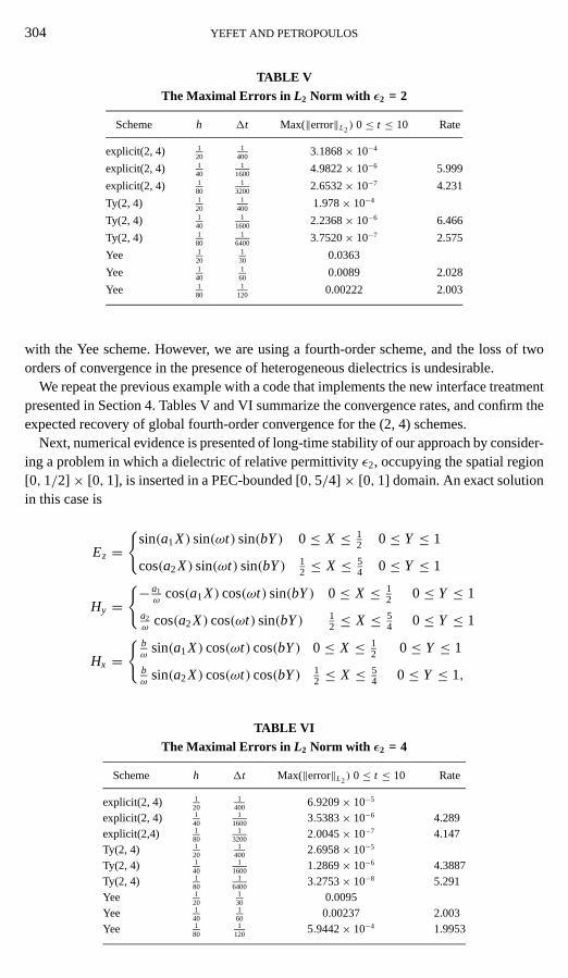
We repeat the previous example with a code that implements the new interface treatmentpresented in Section 4. Tables V and VI summarize the convergence rates, and confirm theexpected recovery of global fourth-order convergence for the (2, 4) schemes.
Next, numerical evidence is presented of long-time stability of our approach by consider-ing a problem in which a dielectric of relative permittivityε2, occupying the spatial region[0, 1/2]× [0, 1], is inserted in a PEC-bounded [0, 5/4]× [0, 1] domain. An exact solutionin this case is
Ez ={
sin(a1X) sin(ωt) sin(bY) 0≤ X ≤ 12 0≤ Y ≤ 1
cos(a2X) sin(ωt) sin(bY) 12 ≤ X ≤ 5
4 0≤ Y ≤ 1
Hy ={− a1
ωcos(a1X) cos(ωt) sin(bY) 0≤ X ≤ 1
2 0≤ Y ≤ 1
a2ω
cos(a2X) cos(ωt) sin(bY) 12 ≤ X ≤ 5
4 0≤ Y ≤ 1
Hx ={ bω
sin(a1X) cos(ωt) cos(bY) 0≤ X ≤ 12 0≤ Y ≤ 1
bω
sin(a2X) cos(ωt) cos(bY) 12 ≤ X ≤ 5
4 0≤ Y ≤ 1,
TABLE VI
The Maximal Errors in L2 Norm with ε2 = 4
Scheme h 1t Max(‖error‖L2) 0≤ t ≤ 10 Rate
explicit(2, 4) 120
1400
6.9209× 10⁻⁵
explicit(2, 4) 140
11600
3.5383× 10⁻⁶ 4.289explicit(2,4) 1
801
32002.0045× 10−7 4.147
Ty(2, 4) 120
1400
2.6958× 10⁻⁵
Ty(2, 4) 140
11600
1.2869× 10⁻⁶ 4.3887Ty(2, 4) 1
801
64003.2753× 10−8 5.291
Yee 120
130
0.0095Yee 1
40160
0.00237 2.003Yee 1
801
1205.9442× 10−4 1.9953
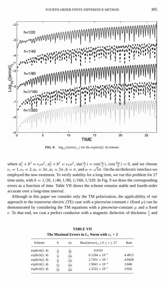
FOURTH-ORDER FINITE-DIFFERENCE METHOD 305
FIG. 9. log10(‖error‖L2) for the explicit(2, 4) scheme.
wherea21 + b2 = ε2ω
2, a22 + b2 = ε1ω
2, sin( a12 ) = cos( a2
2 ), cos( 5a24 ) = 0, and we choose
ε1 = 1,ε2 = 2,a1 = 3π , a2 = 2π , b = π , andω = √5π . On the air/dielectric interface weemployed the new treatment. To verify stability for a long time, we run this problem for 27time units, withh = 1/20, 1/40, 1/80, 1/160, 1/320. In Fig. 9 we draw the correspondingerrors as a function of time. Table VII shows the scheme remains stable and fourth-orderaccurate over a long-time interval.
Although in this paper we consider only the TM polarization, the applicability of ourapproach to the transverse electric (TE) case with a piecewise-constantε (fixedµ) can bedemonstrated by considering the TM equations with a piecewise-constantµ and a fixedε. To that end, we coat a perfect conductor with a magnetic dielectric of thickness1
2 and
TABLE VII
The Maximal Errors in L2 Norm with ε2 = 2
Scheme h 1t Max(‖error‖L2) 0≤ t ≤ 27 Rate
explicit(2, 4) 120
1400
0.0101explicit(2, 4) 1
401
16006.1264× 10−4 4.4815
explicit(2, 4) 180
13200
2.7431× 10⁻⁵ 4.0428explicit(2, 4) 1
1601
32001.9041× 10−6 3.848
explicit(2, 4) 1320
13200
1.2522× 10⁻⁷ 3.926
306 YEFET AND PETROPOULOS
TABLE VIII
The Maximal Errors in L2 Norm with µ2 = 2
Scheme h 1t Max(‖error‖L2) 0≤ t ≤ 10 Rate
explicit(2, 4) 120
1400
0.0021explicit(2, 4) 1
401
16001.4010× 10−4 3.9059
explicit(2, 4) 180
13200
5.2597× 10⁻⁶ 4.7353
relative permeabilityµ2 = 2(µ1 = 1), using the geometry of the previous example. Weused our interface treatment presented in Section 4, and placed the magnetic interface onan electric node. Table VIII summarizes the convergence rate and confirms our scheme’sfourth-order accuracy and stability.
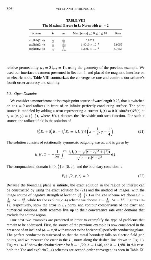
5.3. Open Domains
We consider a monochromatic isotropic point source of wavelength 0.25, that is switchedon at t = 0 and radiates in front of an infinite perfectly conducting surface. The pointsource is modeled by adding a term representing a currentIz(t) = 0.01 sin(8π t)H(t) atrs = (x, y) = ( 1
4,14), where H(t) denotes the Heaviside unit-step function. For such a
source, the radiated field is the solution of
∂2x Ez+ ∂2
y Ez− ∂2t Ez = ∂t Iz(t)δ
(x − 1
4, y− 1
4
). (21)
The solution consists of rotationally symmetric outgoing waves, and is given by
Ez(r, t) = − 1
2π
∫ ∞0
∂t Iz(t −√|r − rs|2+ ξ2))√
|r − rs|2+ ξ2dξ.
The computational domain is [0, 12] × [0, 1
2], and the boundary condition is
Ez(1/2, y, t) = 0. (22)
Because the bounding plane is infinite, the exact solution in the region of interest canbe constructed by using the exact solution for (21) and the method of images, with theimage source of negative strength at location( 3
4,14). For the Yee scheme we chooseh =
140,1t = 2h
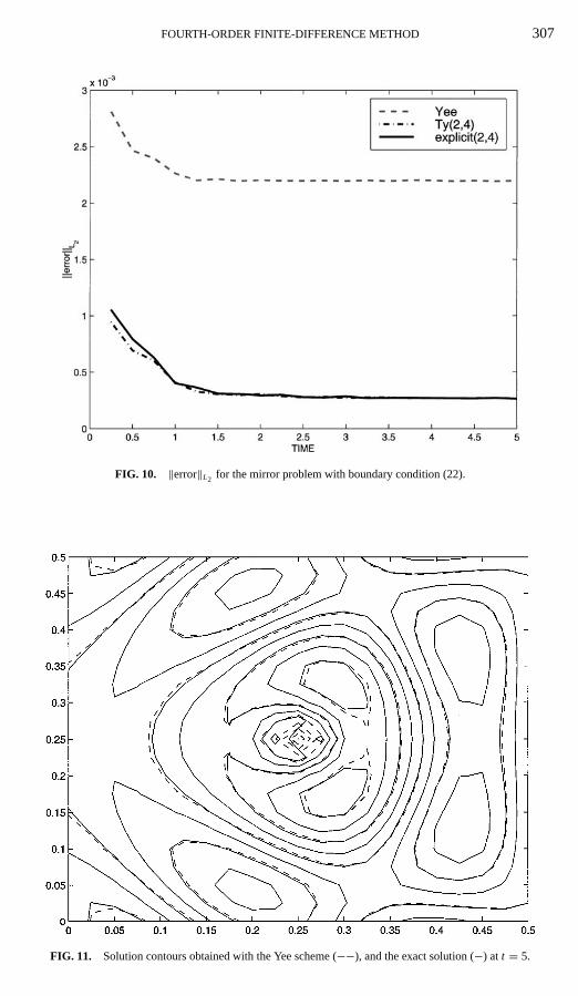
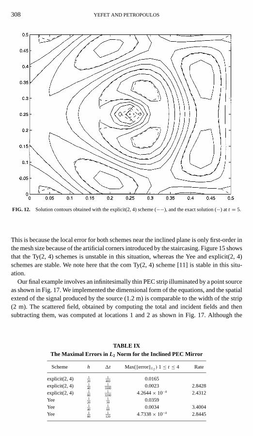
3 , while for the explicit(2, 4) scheme we chooseh = 140,1t = h2. Figures 10–
12, respectively, show the error inL2 norm, and contour comparisons of the exact andnumerical solutions. Both schemes live up to their convergence rate over domains thatexclude the source region.
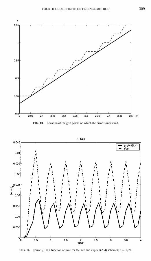
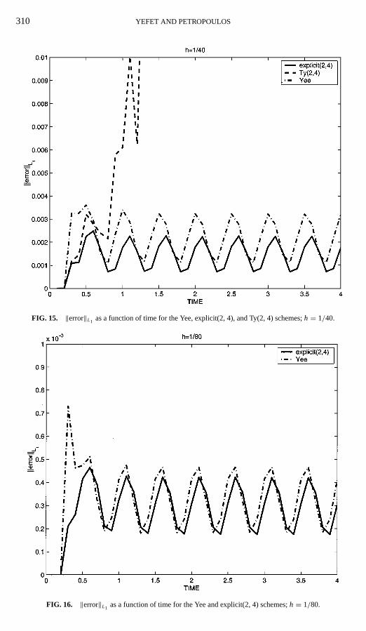
Our next two examples are presented in order to exemplify the type of problems thatremain to be addressed. First, the source of the previous example is now considered in thepresence of an inclined(φ = π/8 with respect to the horizontal) perfectly conducting plane.The perfect conductor is staircased so that the metal boundary falls on electric field gridpoints, and we measure the error in theL1 norm along the dashed line drawn in Fig. 13.Figures 14–16 show the obtained error forh = 1/20,h = 1/40, andh = 1/80. In this case,both the Yee and explicit(2, 4) schemes are second-order convergent as seen in Table IX.
FOURTH-ORDER FINITE-DIFFERENCE METHOD 307
FIG. 10. ‖error‖L2 for the mirror problem with boundary condition (22).
FIG. 11. Solution contours obtained with the Yee scheme (−−), and the exact solution (−) at t = 5.
308 YEFET AND PETROPOULOS
FIG. 12. Solution contours obtained with the explicit(2, 4) scheme (−−), and the exact solution (−) at t = 5.
This is because the local error for both schemes near the inclined plane is only first-order inthe mesh size because of the artificial corners introduced by the staircasing. Figure 15 showsthat the Ty(2, 4) schemes is unstable in this situation, whereas the Yee and explicit(2, 4)schemes are stable. We note here that the com Ty(2, 4) scheme [11] is stable in this situ-ation.
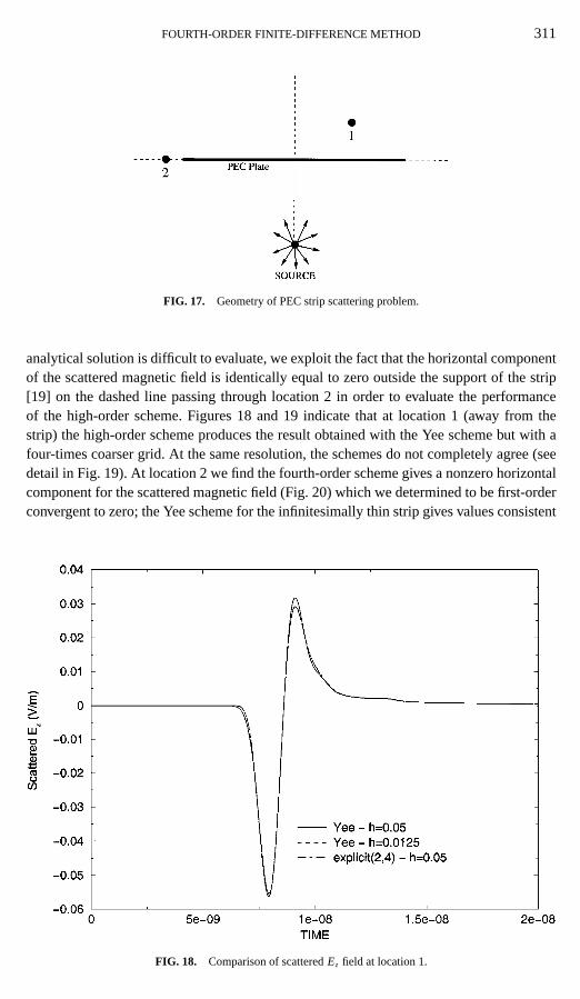
Our final example involves an infinitesimally thin PEC strip illuminated by a point sourceas shown in Fig. 17. We implemented the dimensional form of the equations, and the spatialextend of the signal produced by the source (1.2 m) is comparable to the width of the strip(2 m). The scattered field, obtained by computing the total and incident fields and thensubtracting them, was computed at locations 1 and 2 as shown in Fig. 17. Although the
TABLE IX
The Maximal Errors in L2 Norm for the Inclined PEC Mirror
Scheme h 1t Max(‖error‖L2) 1≤ t ≤ 4 Rate
explicit(2, 4) 120
1400
0.0165explicit(2, 4) 1
401
16000.0023 2.8428
explicit(2, 4) 180
13200
4.2644× 10⁻⁴ 2.4312Yee 1
20130
0.0359Yee 1
40160
0.0034 3.4004Yee 1
801
1204.7338× 10−4 2.8445
FOURTH-ORDER FINITE-DIFFERENCE METHOD 309
FIG. 13. Location of the grid points on which the error is measured.
FIG. 14. ‖error‖L1 as a function of time for the Yee and explicit(2, 4) schemes;h = 1/20.
310 YEFET AND PETROPOULOS
FIG. 15. ‖error‖L1 as a function of time for the Yee, explicit(2, 4), and Ty(2, 4) schemes;h = 1/40.
FIG. 16. ‖error‖L1 as a function of time for the Yee and explicit(2, 4) schemes;h = 1/80.
FOURTH-ORDER FINITE-DIFFERENCE METHOD 311
FIG. 17. Geometry of PEC strip scattering problem.
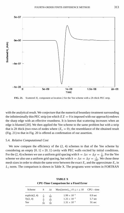
analytical solution is difficult to evaluate, we exploit the fact that the horizontal componentof the scattered magnetic field is identically equal to zero outside the support of the strip[19] on the dashed line passing through location 2 in order to evaluate the performanceof the high-order scheme. Figures 18 and 19 indicate that at location 1 (away from thestrip) the high-order scheme produces the result obtained with the Yee scheme but with afour-times coarser grid. At the same resolution, the schemes do not completely agree (seedetail in Fig. 19). At location 2 we find the fourth-order scheme gives a nonzero horizontalcomponent for the scattered magnetic field (Fig. 20) which we determined to be first-orderconvergent to zero; the Yee scheme for the infinitesimally thin strip gives values consistent
FIG. 18. Comparison of scatteredEz field at location 1.

312 YEFET AND PETROPOULOS
FIG. 19. Detail from Fig. 18.
FIG. 20. ScatteredHx component at location 2 for the explicit(2, 4) scheme.
FOURTH-ORDER FINITE-DIFFERENCE METHOD 313
FIG. 21. ScatteredHx component at location 2 for the Yee scheme with a 2h-thick PEC strip.
with the analytical result. We conjecture that the numerical boundary treatment surroundingthe infinitesimally thin PEC strip (on whichE Z = 0 is imposed with our approach) endowsthe sharp edge with an effective roundness. It is known that scattering increases when anedge is blunted [20]. We then applied the Yee scheme to the same problem but with a stripthat is 2h thick (two rows of nodes where(Ez = 0); the resemblance of the obtained result(Fig. 21) to that in Fig. 20 is offered as confirmation of our assertion.
5.4. Relative Computational Cost
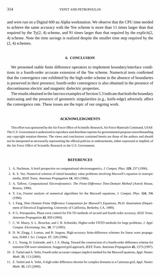
We now compare the efficiency of the (2, 4) schemes to that of the Yee scheme byconsidering an empty [0, 1]× [0, 1] cavity with PEC walls excited by initial conditions.For the (2, 4) schemes we use a uniform grid spacing withh = 1x = 1y = 1
30. For the Yeescheme we also use a uniform grid spacing, but withh = 1x = 1y = 1
240. We chose thesemesh sizes in order to obtain the same error between the exactEz and the approximateEz inL2 norm. The comparison is shown in Table X. The programs were written in FORTRAN
TABLE X
CPU-Time Comparison for a Fixed Error
Scheme h 1t Max(‖error‖L2) 0≤ t ≤ 10 CPU—time
explicit(2, 4) 130
1900
1.99× 10⁻³ 0.9 secTy(2, 4) 1
301
9001.25× 10−3 5.7 sec
Yee 1240
1360
1.31× 10⁻³ 91 sec
314 YEFET AND PETROPOULOS
and were run on a Digital 600 au Alpha workstation. We observe that the CPU time neededto achieve the same accuracy with the Yee scheme is more than 11 times larger than thatrequired by the Ty(2, 4) scheme, and 91 times larger than that required by the explicit(2,4) scheme. Note the time savings is realized despite the smaller time step required by the(2, 4) schemes.
6. CONCLUSION
We presented stable finite difference operators to implement boundary/interface condi-tions in a fourth-order accurate extension of the Yee scheme. Numerical tests confirmedthat the convergence rate exhibited by the high-order scheme in the absence of boundariesis preserved in their presence; fourth-order convergence is also obtained in the presence ofdiscontinuous electric and magnetic dielectric properties.
The results obtained in the last two examples of Section 5.3 indicate that both the boundarystaircasing and the presence of geometric singularities (e.g., knife-edge) adversely affectthe convergence rate. These issues are the topic of our ongoing work.
ACKNOWLEDGMENTS
This effort was sponsored by the Air Force Office of Scientific Research, Air Force Materials Command, USAF.The U.S. Government is authorized to reproduce and distribute reprints for governmental purposes notwithstandingany copyright notation thereon. The views and conclusions contained herein are those of the authors and shouldnot be interpreted as necessarily representing the official policies or endorsements, either expressed or implied, ofthe Air Force Office of Scientific Research or the U.S. Government.
REFERENCES
1. A. Nachman, A brief perspective on computational electromagnetics,J. Comput. Phys.129, 237 (1996).
2. K. S. Yee, Numerical solution of initial boundary value problems involving Maxwell’s equation in isotropicmedia,IEEE Trans. Antennas Propagation14, 302 (1966).
3. A. Taflove,Computational Electrodynamics: The Finite-Difference Time-Domain Method(Artech House,Boston, 1996).
4. Y. Liu, Fourier analysis of numerical algorithms for the Maxwell equations,J. Comput. Phys.124, 396(1996).
5. J. Fang,Time Domain Finite Difference Computation for Maxwell’s Equations, Ph.D. dissertation (Depart-ment of Electrical Engineering, University of California, Berkeley, CA, 1989).
6. P. G. Petropoulos, Phase error control for FD-TD methods of second and fourth order accuracy,IEEE Trans.Antennas Propagation42, 859 (1994).
7. C. W. Manry, S. L. Broschat, and J. B. Schneider, Higher-order FDTD methods for large problems,J. Appl.Comput. Electromag. Soc.10, 17 (1995).
8. D. W. Zingg, J. Lomax, and H. Jurgens, High-accuracy finite-difference schemes for linear wave propaga-tion, SIAM J. Sci. Comput.17, 328 (1996).
9. J. L. Young, D. Gaitonde, and J. J. S. Shang, Toward the construction of a fourth-order difference scheme fortransient EM wave simulation: Staggered grid approach,IEEE Trans. Antennas Propagation45, 1573 (1997).
10. E. Turkel and A. Yefet, Fourth order accurate compact implicit method for the Maxwell quations,Appl. Numer.Math.33, 113 (2000).
11. E. Turkel and A. Yefet, A high order difference shceme for complex domains in a Cartesian grid,Appl. Numer.Math.33, 125 (2000).
FOURTH-ORDER FINITE-DIFFERENCE METHOD 315
12. J. S. Shang, High-order compact-difference schemes for time-dependent Maxwell equations,J. Comput. Phys.153, 312 (1999).
13. D. Gottlieb and B. Yang, Comparisons of staggered and non-Staggered schemes for Maxwell’s equations,12th Ann. Rev. Progress Appl. Comput. Electromag.2, 1122 (1996).
14. M. K. Carpenter, D. Gottlieb, and S. Abarbanel, The stability of numerical boundary treatments for compacthigh-order finite-difference schemes,J. Comput. Phys.108, 272 (1993).
15. K. H. Dridi, J. S. Hesthaven, and A. Ditkowski, Staircase free finite-difference time-domain formulation forarbitrary material distributions in general geometries, submitted for publication.
16. A. Ditkowski, K. H. Dridi, and J. S. Hesthaven, Stable Cartesian grid methods for Maxwell’s equations incomplex geometries. I. Second order schemes, submitted for publication.
17. C. Zhang and R. J. LeVeque, The immersed interface method for acoustic wave equations with discontinuouscoefficients,Wave Motion25, 237 (1997).
18. M. Ghrist, B. Fornberg, and T. A. Driscoll, Staggered time integrators for wave equations,SIAM J. Numer.Anal.38, 718 (2000).
19. J. J. Bowman, T. B. A. Senior, and P. L. E. Uslenghi, Eds.,Electromagnetic and Acoustic Scattering by SimpleShapes(North-Holland, Amsterdam, 1969).
20. K. M. Mitzner, K. J. Kaplin, and J. F. Cashen, How scattering increases as an edge is blunted: The case ofan electric field parallel to the edge, inRecent Advances in Electromagnetic Theory, edited by H. N. Kritikosand D. L. Jaggard (Springer-Verlag, New York, 1990), pp. 319–338.
Related Documents


