A stabilized finite element method using a discontinuous level set approach for solving two phase incompressible flows Emilie Marchandise a,c, * , Jean-Franc ¸ois Remacle a,b a Universite ´ catholique de Louvain, Department of Civil Engineering, Place du Levant 1, 1348 Louvain-la-Neuve, Belgium b Center for Systems Engineering and Applied Mechanics (CESAME), Universite ´ catholique de Louvain, 1348 Louvain-la-Neuve, Belgium c Fonds National, de la Recherche Scientifique, rue d’Egmont 5, 1000 Bruxelles, Belgium Received 31 October 2005; received in revised form 18 April 2006; accepted 24 April 2006 Available online 15 June 2006 Abstract A numerical method for the simulation of three-dimensional incompressible two-phase flows is presented. The proposed algorithm combines an implicit pressure stabilized finite element method for the solution of incompressible two-phase flow problems with a level set method implemented with a quadrature-free discontinuous Galerkin (DG) method [E. Marchan- dise, J.-F. Remacle, N. Chevaugeon, A quadrature free discontinuous Galerkin method for the level set equation, Journal of Computational Physics 212 (2006) 338–357]. The use of a fast contouring algorithm [N. Chevaugeon, E. Marchandise, C. Geuzaine, J.-F. Remacle, Efficient visualization of high order finite elements, International Journal for Numerical Methods in Engineering] permits us to localize the interface accurately. By doing so, we can compute the discontinuous integrals without neither introducing an interface thickness nor reinitializing the level set. The capability of the resulting algorithm is demonstrated with ‘‘large scale’’ numerical examples (free surface flows: dam break, sloshing) and ‘‘small scale’’ ones (two phase Poiseuille, Rayleigh–Taylor instability). Ó 2006 Elsevier Inc. All rights reserved. Keywords: Two-phase flow model; Free surface; Level set; 3D incompressible Navier–Stokes; Discontinuous Galerkin 1. Introduction The study of two phase flows covers a wide range of engineering and environmental flows, including small- scale bubble dynamics, wave mechanics, open channel flows, flows around a ship or structure. The main challenge for solving time-dependent two-phase flow problems in three dimensions is to provide an accurate representation of the interface that separates the two different fluids. This involves the tracking of a discon- tinuity in the material properties like density and viscosity. The principal computational methods used to solve incompressible two-phase flows are the front tracking methods [3–7], and the front capturing methods (volume of fluid [8,9] and level set [10,11]). 0021-9991/$ - see front matter Ó 2006 Elsevier Inc. All rights reserved. doi:10.1016/j.jcp.2006.04.015 DOI of original article: 10.1016/j.jcp.2005.07.006. * Corresponding author. Tel.: +32 1047 2061; fax: +32 1047 2179. E-mail address: [email protected] (E. Marchandise). Journal of Computational Physics 219 (2006) 780–800 www.elsevier.com/locate/jcp

Welcome message from author
This document is posted to help you gain knowledge. Please leave a comment to let me know what you think about it! Share it to your friends and learn new things together.
Transcript
Journal of Computational Physics 219 (2006) 780–800
www.elsevier.com/locate/jcp
A stabilized finite element method using a discontinuous levelset approach for solving two phase incompressible flows
Emilie Marchandise a,c,*, Jean-Francois Remacle a,b
a Universite catholique de Louvain, Department of Civil Engineering, Place du Levant 1, 1348 Louvain-la-Neuve, Belgiumb Center for Systems Engineering and Applied Mechanics (CESAME), Universite catholique de Louvain, 1348 Louvain-la-Neuve, Belgium
c Fonds National, de la Recherche Scientifique, rue d’Egmont 5, 1000 Bruxelles, Belgium
Received 31 October 2005; received in revised form 18 April 2006; accepted 24 April 2006Available online 15 June 2006
Abstract
A numerical method for the simulation of three-dimensional incompressible two-phase flows is presented. The proposedalgorithm combines an implicit pressure stabilized finite element method for the solution of incompressible two-phase flowproblems with a level set method implemented with a quadrature-free discontinuous Galerkin (DG) method [E. Marchan-dise, J.-F. Remacle, N. Chevaugeon, A quadrature free discontinuous Galerkin method for the level set equation, Journalof Computational Physics 212 (2006) 338–357]. The use of a fast contouring algorithm [N. Chevaugeon, E. Marchandise,C. Geuzaine, J.-F. Remacle, Efficient visualization of high order finite elements, International Journal for NumericalMethods in Engineering] permits us to localize the interface accurately. By doing so, we can compute the discontinuousintegrals without neither introducing an interface thickness nor reinitializing the level set.
The capability of the resulting algorithm is demonstrated with ‘‘large scale’’ numerical examples (free surface flows: dambreak, sloshing) and ‘‘small scale’’ ones (two phase Poiseuille, Rayleigh–Taylor instability).� 2006 Elsevier Inc. All rights reserved.
Keywords: Two-phase flow model; Free surface; Level set; 3D incompressible Navier–Stokes; Discontinuous Galerkin
1. Introduction
The study of two phase flows covers a wide range of engineering and environmental flows, including small-scale bubble dynamics, wave mechanics, open channel flows, flows around a ship or structure. The mainchallenge for solving time-dependent two-phase flow problems in three dimensions is to provide an accuraterepresentation of the interface that separates the two different fluids. This involves the tracking of a discon-tinuity in the material properties like density and viscosity.
The principal computational methods used to solve incompressible two-phase flows are the front trackingmethods [3–7], and the front capturing methods (volume of fluid [8,9] and level set [10,11]).
0021-9991/$ - see front matter � 2006 Elsevier Inc. All rights reserved.
doi:10.1016/j.jcp.2006.04.015
DOI of original article: 10.1016/j.jcp.2005.07.006.* Corresponding author. Tel.: +32 1047 2061; fax: +32 1047 2179.
E-mail address: [email protected] (E. Marchandise).
E. Marchandise, J.-F. Remacle / Journal of Computational Physics 219 (2006) 780–800 781
A successful approach to deal with two phase flows, especially in the presence of topological changes, isthe level set method [10]. Application of level sets in two-phase flow calculations have been extensivelydescribed by Sussman, Smereka and Osher in [11–13] and used by among others [14–17]. The level set func-tion is able to represent an arbitrary number of bubbles or drops interfaces and complex changes of topol-ogy are naturally taken into account by the method. The level set function /ð~x; tÞ is defined to be a smoothfunction that is positive in one region and negative in the other. The implicit surface /ð~x; tÞ ¼ 0 representsthe current position of an interface. This interface is advected by a vector field uð~x; tÞ that is, in case of two-phase flows, the solution of the Navier–Stokes equations. The elementary advection equation for interfaceevolution is:
ot/þ u � r/ ¼ 0: ð1Þ
In [1], we have developed a high order quadrature free Runge–Kutta discontinuous Galerkin (DG) method tosolve the level set equation (1) in space and time. The method was compared with classical Hamilton–JacobiENO/WENO methods [13,18–20] and showed to be computationally effective and mass conservative. Besides,we showed that there was no need to reinitialize the level set.Level sets are representing a fluid interface in an implicit manner. The main advantage of this approach isthat the underlying computational mesh does not conform to the interface. Hence, discontinuous integralshave to be computed in the fluid formulation because both viscosities and densities are discontinuous in allthe elements crossed by the interface. The most common approach is to define a zone of thickness 2� in thevicinity of the interface (j/j < �) and to smooth the discontinuous density and viscosity over this thickness[11,17,21–23]. Smoothing physical parameters in the interfacial zone may be the cause of two problems.The first one is the introduction of non-physical densities and viscosities in the smoothed region, leading topossible thermodynamical aberrations [24]. The second problem is the obligation to keep the interface thick-ness constant in time. For ensuring that the smoothed region has a constant thickness, one has to reinitializethe level set so that it remains a distance function. In this work, we rather adopt a discontinuous approach[25,26] to compute the discontinuous integrals. The use of a recursive contouring algorithm [2] allows to local-ize the interface accurately. Consequently, we are able to compute the discontinuous integrals with a very highlevel of accuracy.
For the computation of the incompressible two-phase Navier–Stokes equations, various numerical methodshave been developed. Among them are the projection methods [27–29], stabilized finite element methods[17,30,31] and artificial compressibility methods [32,33]. A key feature of stabilized methods is that they haveproved to be LBB stable and to have good convergence properties [34,35].
In this work, we present a stabilized finite element method for computing flows in both phases and combineit with a discontinuous Galerkin level set method for computing the interface motion. The overall algorithmavoids the cost of the renormalization of the level set as well as the introduction of a non-physical interfacethickness and exhibits good mass conservation properties.
The outline of this paper is as follows: we first present the governing equations in Section 2. Section 3 isdevoted to the description of our computational method. We present the Navier–Stokes solver and the cou-pling with the discontinuous Galerkin method for the level set equation. Section 4 gives numerical examples toverify accuracy, stability and convergence properties.
2. Governing equation
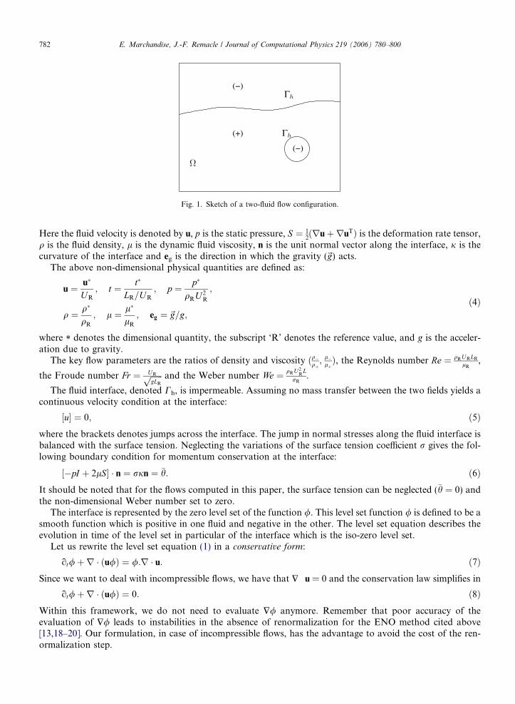
In the present work, the three-dimensional flow field of two non-miscible laminar incompressible fluids iscalculated. The two fluids are denoted respectively by (+) and (�) and have distinct viscosity and density(q+,l+) and (q�,l�). Fig. 1 shows an illustration of a configuration with two fluids.
The solution in both phases, denoted as phase (+) and phase (�), are obtained simultaneously. The non-dimensional equations are given by the incompressible Navier–Stokes equations:
Du
Dt¼ � rp
qð/Þ þ1
qð/Þ1
Rer � ð2lð/ÞSÞ þ eg
Fr2þ jn
We; ð2Þ
r � u ¼ 0: ð3Þ
(+)
Ω
Γ
Γ
Fig. 1. Sketch of a two-fluid flow configuration.
782 E. Marchandise, J.-F. Remacle / Journal of Computational Physics 219 (2006) 780–800
Here the fluid velocity is denoted by u, p is the static pressure, S ¼ 12ðruþruTÞ is the deformation rate tensor,
q is the fluid density, l is the dynamic fluid viscosity, n is the unit normal vector along the interface, j is thecurvature of the interface and eg is the direction in which the gravity (~g) acts.
The above non-dimensional physical quantities are defined as:
u ¼ u�
UR
; t ¼ t�
LR=U R
; p ¼ p�
qRU 2R
;
q ¼ q�
qR
; l ¼ l�
lR
; eg ¼~g=g;ð4Þ
where * denotes the dimensional quantity, the subscript ‘R’ denotes the reference value, and g is the acceler-ation due to gravity.
The key flow parameters are the ratios of density and viscosity ðq�qþ;l�lþÞ, the Reynolds number Re ¼ qRURLR
lR,
the Froude number Fr ¼ URffiffiffiffiffiffigLR
p and the Weber number We ¼ qRU2R
L
rR.
The fluid interface, denoted Ch, is impermeable. Assuming no mass transfer between the two fields yields acontinuous velocity condition at the interface:
½u� ¼ 0; ð5Þ
where the brackets denotes jumps across the interface. The jump in normal stresses along the fluid interface isbalanced with the surface tension. Neglecting the variations of the surface tension coefficient r gives the fol-lowing boundary condition for momentum conservation at the interface:½�pI þ 2lS� � n ¼ rjn ¼ �h: ð6Þ
It should be noted that for the flows computed in this paper, the surface tension can be neglected (�h ¼ 0) andthe non-dimensional Weber number set to zero.The interface is represented by the zero level set of the function /. This level set function / is defined to be asmooth function which is positive in one fluid and negative in the other. The level set equation describes theevolution in time of the level set in particular of the interface which is the iso-zero level set.
Let us rewrite the level set equation (1) in a conservative form:
ot/þr � ðu/Þ ¼ /:r � u: ð7Þ
Since we want to deal with incompressible flows, we have that $ Æ u = 0 and the conservation law simplifies inot/þr � ðu/Þ ¼ 0: ð8Þ
Within this framework, we do not need to evaluate $/ anymore. Remember that poor accuracy of theevaluation of $/ leads to instabilities in the absence of renormalization for the ENO method cited above[13,18–20]. Our formulation, in case of incompressible flows, has the advantage to avoid the cost of the ren-ormalization step.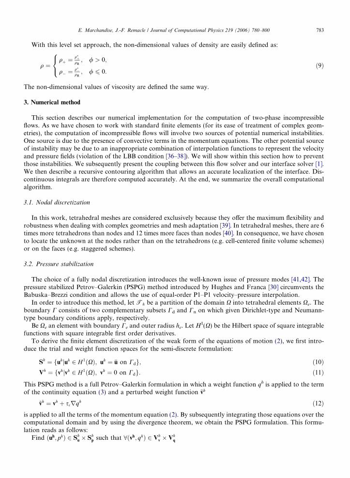
E. Marchandise, J.-F. Remacle / Journal of Computational Physics 219 (2006) 780–800 783
With this level set approach, the non-dimensional values of density are easily defined as:
q ¼qþ ¼
q�þqR; / > 0;
q� ¼q��qR; / 6 0:
8<: ð9Þ
The non-dimensional values of viscosity are defined the same way.
3. Numerical method
This section describes our numerical implementation for the computation of two-phase incompressibleflows. As we have chosen to work with standard finite elements (for its ease of treatment of complex geom-etries), the computation of incompressible flows will involve two sources of potential numerical instabilities.One source is due to the presence of convective terms in the momentum equations. The other potential sourceof instability may be due to an inappropriate combination of interpolation functions to represent the velocityand pressure fields (violation of the LBB condition [36–38]). We will show within this section how to preventthose instabilities. We subsequently present the coupling between this flow solver and our interface solver [1].We then describe a recursive contouring algorithm that allows an accurate localization of the interface. Dis-continuous integrals are therefore computed accurately. At the end, we summarize the overall computationalalgorithm.
3.1. Nodal discretization
In this work, tetrahedral meshes are considered exclusively because they offer the maximum flexibility androbustness when dealing with complex geometries and mesh adaptation [39]. In tetrahedral meshes, there are 6times more tetrahedrons than nodes and 12 times more faces than nodes [40]. In consequence, we have chosento locate the unknown at the nodes rather than on the tetrahedrons (e.g. cell-centered finite volume schemes)or on the faces (e.g. staggered schemes).
3.2. Pressure stabilization
The choice of a fully nodal discretization introduces the well-known issue of pressure modes [41,42]. Thepressure stabilized Petrov–Galerkin (PSPG) method introduced by Hughes and Franca [30] circumvents theBabuska–Brezzi condition and allows the use of equal-order P1–P1 velocity–pressure interpolation.
In order to introduce this method, let Th be a partition of the domain X into tetrahedral elements Xe. Theboundary C consists of two complementary subsets Cd and Cn on which given Dirichlet-type and Neumann-type boundary conditions apply, respectively.
Be Xe an element with boundary Ce and outer radius he. Let H1(X) be the Hilbert space of square integrablefunctions with square integrable first order derivatives.
To derive the finite element discretization of the weak form of the equations of motion (2), we first intro-duce the trial and weight function spaces for the semi-discrete formulation:
Sh ¼ fuhjuh 2 H 1ðXÞ; uh ¼ �u on Cdg; ð10ÞVh ¼ fvhjvh 2 H 1ðXÞ; vh ¼ 0 on Cdg: ð11Þ
This PSPG method is a full Petrov–Galerkin formulation in which a weight function qh is applied to the termof the continuity equation (3) and a perturbed weight function ~vh
~vh ¼ vh þ s�rqh ð12Þ
is applied to all the terms of the momentum equation (2). By subsequently integrating those equations over thecomputational domain and by using the divergence theorem, we obtain the PSPG formulation. This formu-lation reads as follows:Find ðuh; phÞ 2 Shu � Sh
p such that 8ðvh; qhÞ 2 Vhv � Vh
q
784 E. Marchandise, J.-F. Remacle / Journal of Computational Physics 219 (2006) 780–800
ZX
otuhvh dvþ
ZX
vhuh � ruh dvþZ
Xrvh l
qReruh dvþ
ZX
vhrph
qdv ¼
ZX
vh eg
Fr2dv; ð13ÞZ
Xqhr � uh dvþ ST ¼ 0: ð14Þ
The stabilization term ST
ST ¼X
e
ZXe
serqhRðph; uhÞ dv ð15Þ
contains the residual of the momentum equation
Rðph; uhÞ ¼ otuh þ ðuh � rÞuh � l
qRer2uh þ 1
qrph � eg
Fr2: ð16Þ
The stabilization parameter s� is of order Oðh2e=mÞ in the diffusion dominated case and of order of OðheÞ in the
advection dominated case [43,44].
3.3. Convective stabilization
It is well known that in the context of finite elements, there is a need to stabilize the advective term. Onepopular possibility is to use the streamline upwind/Petrov–Galerkin (SUPG) formulation. In this work, wehave rather chosen to use an upwind finite volume stabilization with the finite volumes being the median cells.This work is based on the one of Barth and Selmin [45,46] in which they show the link between the standardfinite element Galerkin formulation on tetrahedral meshes and the finite volume formulation with control vol-umes being the median cells. Those median cells are obtained by connecting the centroid of each face of thesurrounding tetrahedrons to the midpoint of the edges of the tetrahedron. We have chosen to use a full upwindmethod when evaluating the convective flux on the faces of this control volume. Those fluxes at the faces of thedual cell are computed using a linear approximation of the variables:
uface ¼ unode þ DxTrunode; ð17Þ
where the nodal gradients $unode are computed with a least square reconstruction method [47].3.4. Coupling between the two solvers
In this section, we describe how we have coupled our two-phase incompressible flow solver with the inter-face solver that is the RK-DG method for the level set equation. First, we have used the same computationalmesh for both solvers.
The flow solver uses continuous linear approximations (N1) for the velocity u while the interface DG solveruses piecewise continuous high order (p) approximations (Np) for the level set /
u ¼X4
i¼1
uiN 1i and / ¼
Xnp
i¼1
/iNpi :
The reason why higher order polynomials are used for discretizing the level set is that Eq. (1) involves $/ andu. We choose a level set for which the gradient is at least in the space of the velocity.
Projection operators are used to project the velocity space to the level set space and conversely. The elemen-tary projection operator P that projects the velocity variable from a polynomial space of order p = a to a spaceof order p = b is given by:
ub ¼ Pua ¼ M�bMabua; ð18Þ
where the mass matrix for the element Xe is given by:Mabij ¼
ZXe
N ai Nb
j dv: ð19Þ
E. Marchandise, J.-F. Remacle / Journal of Computational Physics 219 (2006) 780–800 785
On the other way, to project the / unknowns to the flows dofs, we take the average of / at the nodes of thetetrahedron. Fig. 2 illustrates the coupling described above.
3.5. Evaluation of the discontinuous integrals
Since the interface is represented implicitly by the zero level set, the computational mesh does not conformwith the interface. It follows that if the density and viscosity are discontinuous across the interface, the twofollowing integrals of Eq. (13) are discontinuous:
ZXe
vhrph
qdv and
ZXe
rvh lqReruh dv: ð20Þ
An accurate localization of the interface enables us to divide the discontinuous integrals into two continuousintegrals and to compute those exactly by numerical integration:
ZXe
vhrph
qdv ¼
ZV þ
vhrph
qþdvþ
ZV �
vhrph
q�dv; ð21ÞZ
Xe
rvh lqReruh dv ¼
ZV þ
rvh lþqþRe
ruh dvþZ
V �
rvh l�q�Re
ruh dv: ð22Þ
The question is how accurately can we determine the shape of the interface? To answer this question, we con-sider a triangular element of coordinates (0, 0) (1, 0) and (0, 1) that is crossed by the interface. Consider thefollowing level set function:
/ðx; yÞ ¼ ðx� 1Þ2 þ y2 � ð0:5Þ2
for which the iso-zero level set (interface) is the circle of radius (1, 0). Remember that we use high order poly-nomials to represent the level set within the interface solver, while within the fluid solver we only keep in mem-ory the nodal values of the level set.
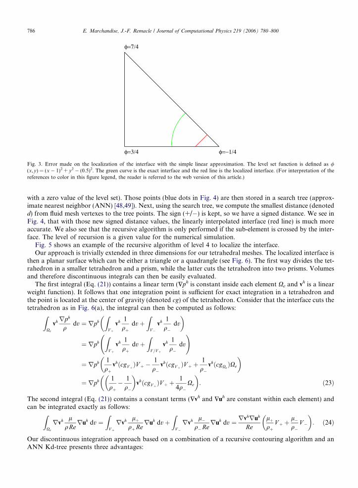
The first idea to localize the interface is to interpolate linearly the iso-zero level set (interface) from thenodal values of the level set. Unfortunately, since the level set (even if initially defined as a distance function)does not remain a distance function throughout the computation, this approach leads to a significant locali-zation error of the interface. Fig. 3 illustrates the error made with the first approach.
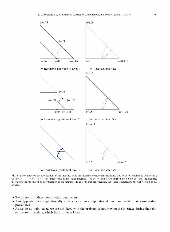
A more accurate approach (illustrated in Fig. 4) is to use the recursive contouring algorithm described in [2]combined with a fast search tree method.
The approach is quite simple. It consists of dividing the elements recursively into sub-elements and per-forms a linear approximation on every edge of those sub-elements to find the points on the interface (points
u,p φ
projection level set
projection velocity
with ρ(φ), μ(φ)
Flow solver Interface solver
Fig. 2. Coupling between flow solver and the interface solver.
φ=7/4
φ=3/4 φ=−1/4
Fig. 3. Error made on the localization of the interface with the simple linear approximation. The level set function is defined as /(x,y) = (x � 1)2 + y2 � (0.5)2. The green curve is the exact interface and the red line is the localized interface. (For interpretation of thereferences to color in this figure legend, the reader is referred to the web version of this article.)
786 E. Marchandise, J.-F. Remacle / Journal of Computational Physics 219 (2006) 780–800
with a zero value of the level set). Those points (blue dots in Fig. 4) are then stored in a search tree (approx-imate nearest neighbor (ANN) [48,49]). Next, using the search tree, we compute the smallest distance (denotedd) from fluid mesh vertexes to the tree points. The sign (+/�) is kept, so we have a signed distance. We see inFig. 4, that with those new signed distance values, the linearly interpolated interface (red line) is much moreaccurate. We also see that the recursive algorithm is only performed if the sub-element is crossed by the inter-face. The level of recursion is a given value for the numerical simulation.
Fig. 5 shows an example of the recursive algorithm of level 4 to localize the interface.Our approach is trivially extended in three dimensions for our tetrahedral meshes. The localized interface is
then a planar surface which can be either a triangle or a quadrangle (see Fig. 6). The first way divides the tet-rahedron in a smaller tetrahedron and a prism, while the latter cuts the tetrahedron into two prisms. Volumesand therefore discontinuous integrals can then be easily evaluated.
The first integral (Eq. (21)) contains a linear term ($ph is constant inside each element Xe and vh is a linearweight function). It follows that one integration point is sufficient for exact integration in a tetrahedron andthe point is located at the center of gravity (denoted cg) of the tetrahedron. Consider that the interface cuts thetetrahedron as in Fig. 6(a), the integral can then be computed as follows:
ZXe
vhrph
qdv ¼ rph
ZV þ
vh 1
qþdvþ
ZV �
vh 1
q�dv
� �
¼ rph
ZV þ
vh 1
qþdvþ
ZV =V þ
vh 1
q�dv
!
¼ rph 1
qþvhðcgV þÞV þ �
1
q�vhðcgV þÞV þ þ
1
q�vhðcgXe
ÞXe
� �
¼ rph 1
qþ� 1
q�
� �vhðcgV þÞV þ þ
1
4q�Xe
� �: ð23Þ
The second integral (Eq. (21)) contains a constant terms ($vh and $uh are constant within each element) andcan be integrated exactly as follows:
ZXe
rvh lqReruh dv ¼
ZV þ
rvh lþqþRe
ruh dvþZ
V �
rvh l�q�Re
ruh dv ¼ rvhruh
Relþqþ
V þ þl�q�
V �
� �: ð24Þ
Our discontinuous integration approach based on a combination of a recursive contouring algorithm and anANN Kd-tree presents three advantages:
φ=3/4 φ=0 φ=−1/4
φ=1/4
φ=1.75
d=0.5
d=1.06
Recursive algorithm of level 1(a) (b)
(a) (b)
(a) (b)
Localized interface.
φ=0 φ=−3/16
φ=−1/8φ=1/16
φ=1/4
d=0.95
d=0.5
Recursive algorithm of level 2 Localized interface.
d=0.5
d=0.914
Recursive algorithm of level 3 Localized interface.
Fig. 4. Error made on the localization of the interface with the recursive contouring algorithm. The level set function is defined as /(x,y) = (x � 1)2 + y2 � (0.5)2. The green curve is the exact interface. The set of points are marked by a blue dot and the localizedinterface is the red line. (For interpretation of the references to color in this figure legend, the reader is referred to the web version of thisarticle.)
E. Marchandise, J.-F. Remacle / Journal of Computational Physics 219 (2006) 780–800 787
� We do not introduce non-physical parameters.� This approach is computationally more efficient in computational time compared to renormalization
procedures.� As we do not reinitialize, we are not faced with the problem of not moving the interface during the reini-
tialization procedure, which leads to mass losses.
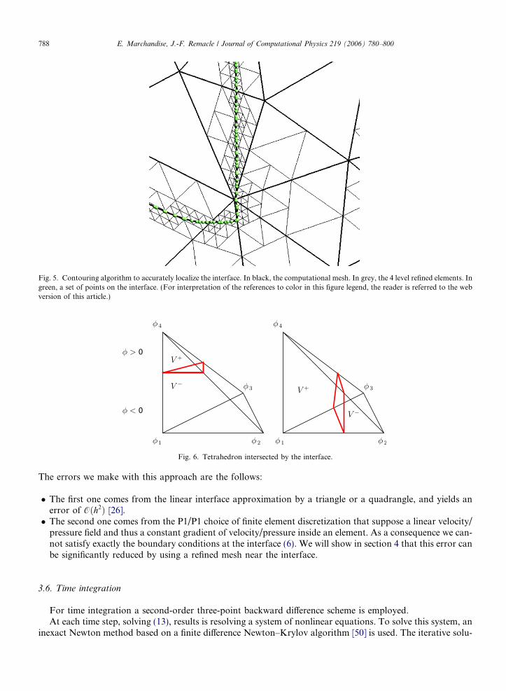
Fig. 5. Contouring algorithm to accurately localize the interface. In black, the computational mesh. In grey, the 4 level refined elements. Ingreen, a set of points on the interface. (For interpretation of the references to color in this figure legend, the reader is referred to the webversion of this article.)
Fig. 6. Tetrahedron intersected by the interface.
788 E. Marchandise, J.-F. Remacle / Journal of Computational Physics 219 (2006) 780–800
The errors we make with this approach are the follows:
� The first one comes from the linear interface approximation by a triangle or a quadrangle, and yields anerror of Oðh2Þ [26].� The second one comes from the P1/P1 choice of finite element discretization that suppose a linear velocity/
pressure field and thus a constant gradient of velocity/pressure inside an element. As a consequence we can-not satisfy exactly the boundary conditions at the interface (6). We will show in section 4 that this error canbe significantly reduced by using a refined mesh near the interface.
3.6. Time integration
For time integration a second-order three-point backward difference scheme is employed.At each time step, solving (13), results is resolving a system of nonlinear equations. To solve this system, an
inexact Newton method based on a finite difference Newton–Krylov algorithm [50] is used. The iterative solu-
E. Marchandise, J.-F. Remacle / Journal of Computational Physics 219 (2006) 780–800 789
tion of the large sparse linear system of equations that arises at each Newton iteration is solved by theGMRES method preconditioned by the RAS [51] algorithm.
3.7. Summary of the algorithm
Our computational approach for numerical modeling of two-phase flows can be summarized as follows.First we initialize all the variables (velocity u, pressure p, level set /). Then,
For each time tn, n = 0,1,2 . . .:
� First solve the Navier–Stokes equation from tn�1 until tn and find a velocity un. This equation is solvedimplicitly for the velocity and pressure variables but uses the previous position of the level set /n�1 to iden-tify the fluid variable such as viscosity and density. To go to step 2, project the velocity field u onto the dofsof the interface solver.� Second advance explicitly the level set (Eq. (8)) from tn�1 until tn using sub-time steps with a linear velocity
varying in time between un�1 until un and find a new position for the level set /n. Then project the level setfunction / onto the dofs of the fluid solver.� Third go back to step 2, with this new position /n and repeat those steps until i/n�1 � /ni < eps.
4. Numerical results and discussion
In this section, the coupling of the incompressible two-phase flow solver and the interface solver describedin the previous section is tested and applied to several 2D and 3D two-phase flows problems. As we are onlyworking with tetrahedral meshes, we use for the computation of the 2D flows a 2D mesh that is extruded overa thin layer in the third dimension.
Our methods were implemented in Standard C++, compiled with GNU g++ v3.3, and run on one CPU ofa 2.4 GHz Intel(R) Pentium(R) 4 with 512 KB of L2 cache.
4.1. Poiseuille two-phase flow
The horizontal stratified flow of two fluids between parallel walls is first considered. For long times a steadysolution is obtained for the two-phase flow problem which can be described by an analytical solution. Thissimple test case does not include any deformation of the interface but is interesting anyway because it allowsto characterize the error due to the evaluation of the discontinuous integrals.
The height of the channel is H = 2 m and the length L = 4 m. The kinematic viscosities of the two fluids are,respectively, m1 = 0.1 and m2 = 0.02 m/s2. The two fluids are assumed to have the same density. The pressures areimposed on the left and right limit of the calculation domain to ensure a pressure difference of Dp = � 2.0 Pa. Theinterface between the two phases is located at the half height of the channel. The numerical solution was obtainedwithin one iteration with a huge time step of 104 s. The residual decreased of 6 orders of magnitude.
The comparison between the analytical and numerical velocity field is depicted at Fig. 8. The solutions havebeen computed for three different structured and unstructured meshes (see Fig. 7) of mesh size h = 0.1. Thefirst mesh 7(a) is structured and build such that the interface between the two phases corresponds with themesh. The second 7(b) is a structured mesh in which the interface cuts the tetrahedron and the third one7(c) is an unstructured mesh that is refined near the interface (h = 0.01).
Table 1 shows the L2 error on the velocity field for those three meshes. We see that, with mesh a, we capturewell the analytical solution while with mesh b, errors are significant. The error comes from the evaluation ofintegral (22). Indeed the boundary conditions are not exactly satisfied. We should have [p] = 0 and ½lou
on� ¼ 0,where the brackets denote the jump at the interface. The first condition is satisfied while the second cannot besatisfied since we have ½ou
on� ¼ 0 and [l] 6¼ 0. This error can be reduced by refining the mesh near the interface.This is done in mesh c.
Another way to reduce the error is to enrich the velocity field with an extended basis (XFEM) whose gra-dient is discontinuous across the interface. This has been done by Chessa and Belytschko in [14,15]. The only
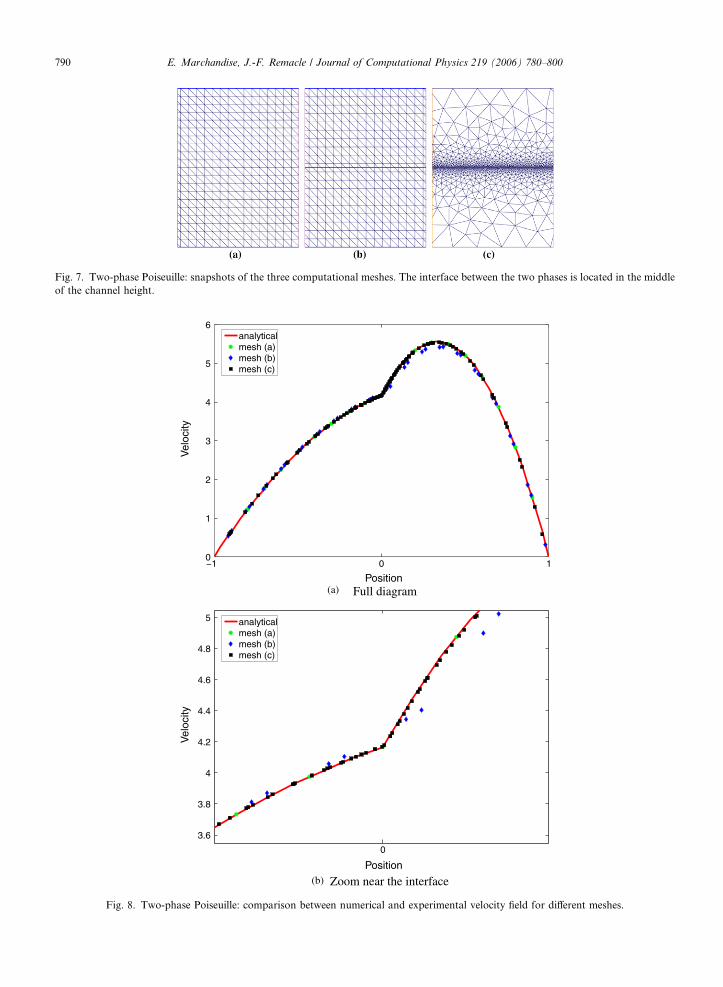
Fig. 7. Two-phase Poiseuille: snapshots of the three computational meshes. The interface between the two phases is located in the middleof the channel height.
0 10
1
2
3
4
5
6
Position
Vel
ocity
analyticalmesh (a)mesh (b)mesh (c)
(a)
(b)
Full diagram
0
3.6
3.8
4
4.2
4.4
4.6
4.8
5
Position
Vel
ocity
analyticalmesh (a)mesh (b)mesh (c)
Zoom near the interface
Fig. 8. Two-phase Poiseuille: comparison between numerical and experimental velocity field for different meshes.
790 E. Marchandise, J.-F. Remacle / Journal of Computational Physics 219 (2006) 780–800
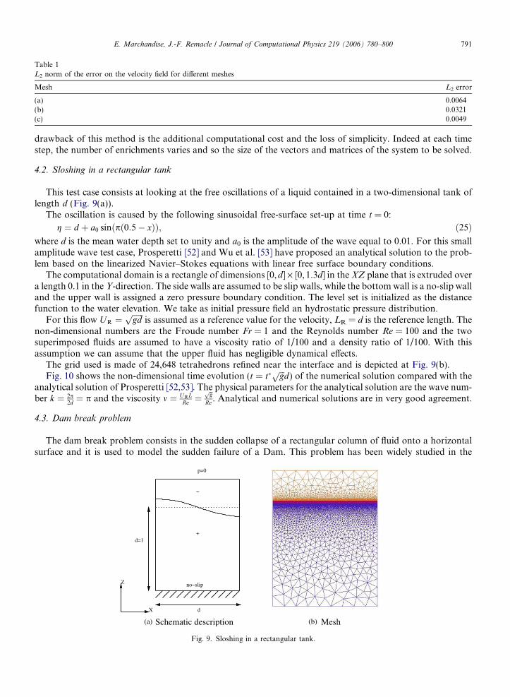
Table 1L2 norm of the error on the velocity field for different meshes
Mesh L2 error
(a) 0.0064(b) 0.0321(c) 0.0049
E. Marchandise, J.-F. Remacle / Journal of Computational Physics 219 (2006) 780–800 791
drawback of this method is the additional computational cost and the loss of simplicity. Indeed at each timestep, the number of enrichments varies and so the size of the vectors and matrices of the system to be solved.
4.2. Sloshing in a rectangular tank
This test case consists at looking at the free oscillations of a liquid contained in a two-dimensional tank oflength d (Fig. 9(a)).
The oscillation is caused by the following sinusoidal free-surface set-up at time t = 0:
g ¼ d þ a0 sinðpð0:5� xÞÞ; ð25Þ
where d is the mean water depth set to unity and a0 is the amplitude of the wave equal to 0.01. For this smallamplitude wave test case, Prosperetti [52] and Wu et al. [53] have proposed an analytical solution to the prob-lem based on the linearized Navier–Stokes equations with linear free surface boundary conditions.The computational domain is a rectangle of dimensions [0,d] · [0, 1.3d] in the XZ plane that is extruded overa length 0.1 in the Y-direction. The side walls are assumed to be slip walls, while the bottom wall is a no-slip walland the upper wall is assigned a zero pressure boundary condition. The level set is initialized as the distancefunction to the water elevation. We take as initial pressure field an hydrostatic pressure distribution.
For this flow U R ¼ffiffiffiffiffiffigdp
is assumed as a reference value for the velocity, LR = d is the reference length. Thenon-dimensional numbers are the Froude number Fr = 1 and the Reynolds number Re = 100 and the twosuperimposed fluids are assumed to have a viscosity ratio of 1/100 and a density ratio of 1/100. With thisassumption we can assume that the upper fluid has negligible dynamical effects.
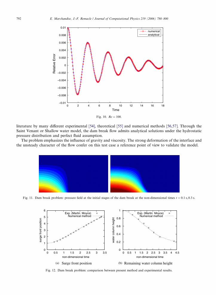
The grid used is made of 24,648 tetrahedrons refined near the interface and is depicted at Fig. 9(b).Fig. 10 shows the non-dimensional time evolution (t ¼ t�
ffiffiffigp
d) of the numerical solution compared with theanalytical solution of Prosperetti [52,53]. The physical parameters for the analytical solution are the wave num-ber k ¼ 2p
2d ¼ p and the viscosity m ¼ URLRe ¼
ffiffigp
Re . Analytical and numerical solutions are in very good agreement.
4.3. Dam break problem
The dam break problem consists in the sudden collapse of a rectangular column of fluid onto a horizontalsurface and it is used to model the sudden failure of a Dam. This problem has been widely studied in the
Z
X
d=1
d
p=0
+
(a) Schematic description (b) Mesh
Fig. 9. Sloshing in a rectangular tank.
0 2 4 6 8 10 12 14 16 18
0
0.002
0.004
0.006
0.008
0.01
Time
Rel
ativ
e E
rror
numericalanalytical
Fig. 10. Re = 100.
792 E. Marchandise, J.-F. Remacle / Journal of Computational Physics 219 (2006) 780–800
literature by many different experimental [54], theoretical [55] and numerical methods [56,57]. Through theSaint Venant or Shallow water model, the dam break flow admits analytical solutions under the hydrostaticpressure distribution and perfect fluid assumption.
The problem emphasizes the influence of gravity and viscosity. The strong deformation of the interface andthe unsteady character of the flow confer on this test case a reference point of view to validate the model.
Fig. 11. Dam break problem: pressure field at the initial stages of the dam break at the non-dimensional times t = 0.1 s,0.3 s.
0
1
2
3
4
5
6
0 0.5 1 1.5 2 2.5 3 3.5
surg
e fr
ont p
ositi
on
non-dimensional time
Exp. (Martin Moyce)Numerical method
0
0.2
0.4
0.6
0.8
1
0 0.5 1 1.5 2 2.5 3 3.5 4 4.5
wat
er c
olum
n he
ight
non-dimensional time
Exp. (Martin Moyce)Numerical method
(a) Surge front position (b) Remaining water column height
Fig. 12. Dam break problem: comparison between present method and experimental results.
E. Marchandise, J.-F. Remacle / Journal of Computational Physics 219 (2006) 780–800 793
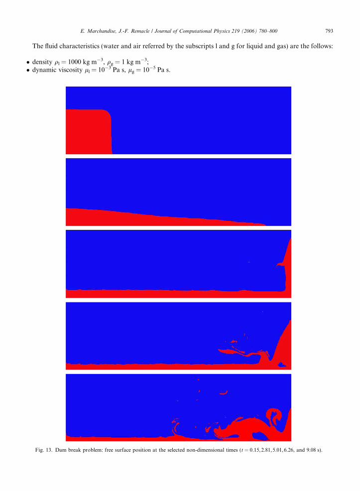
The fluid characteristics (water and air referred by the subscripts l and g for liquid and gas) are the follows:
� density ql = 1000 kg m�3, qg = 1 kg m�3;� dynamic viscosity ll = 10�3 Pa s, lg = 10�5 Pa s.
Fig. 13. Dam break problem: free surface position at the selected non-dimensional times (t = 0.15,2.81,5.01,6.26, and 9.08 s).
794 E. Marchandise, J.-F. Remacle / Journal of Computational Physics 219 (2006) 780–800
The Reynolds number is 40,000. Non-slip boundary conditions are applied to all the walls, therefore the watercolumn collapses under gravity.
The calculation domain is described by the length L = 6 m and the height H = 1.5 m. The height of thewater column is hl = 1 m. The mesh is unstructured and made of 10,218 nodes.
Fig. 11 depicts the pressure field at the initial stages of the dam break.The history of the dimensionless horizontal displacement of the water front is shown in Fig. 12. For com-
parison the experimental values from Martin and Moyce [54] are added to the diagram. In this diagram, thetime is non-dimensionalized by t ¼
ffiffiffiffiffiffiffiffiffihl=g
p.
Finally, Fig. 13 displays snapshots of the free surface position at selected times.
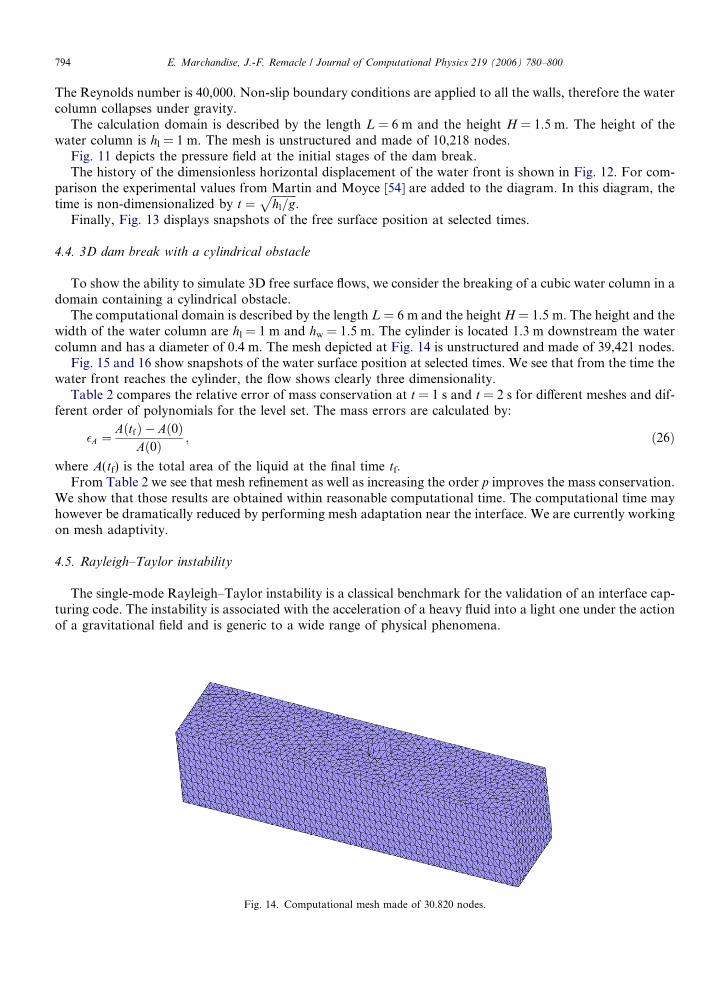
4.4. 3D dam break with a cylindrical obstacle
To show the ability to simulate 3D free surface flows, we consider the breaking of a cubic water column in adomain containing a cylindrical obstacle.
The computational domain is described by the length L = 6 m and the height H = 1.5 m. The height and thewidth of the water column are hl = 1 m and hw = 1.5 m. The cylinder is located 1.3 m downstream the watercolumn and has a diameter of 0.4 m. The mesh depicted at Fig. 14 is unstructured and made of 39,421 nodes.
Fig. 15 and 16 show snapshots of the water surface position at selected times. We see that from the time thewater front reaches the cylinder, the flow shows clearly three dimensionality.
Table 2 compares the relative error of mass conservation at t = 1 s and t = 2 s for different meshes and dif-ferent order of polynomials for the level set. The mass errors are calculated by:
�A ¼AðtfÞ � Að0Þ
Að0Þ ; ð26Þ
where A(tf) is the total area of the liquid at the final time tf.From Table 2 we see that mesh refinement as well as increasing the order p improves the mass conservation.
We show that those results are obtained within reasonable computational time. The computational time mayhowever be dramatically reduced by performing mesh adaptation near the interface. We are currently workingon mesh adaptivity.
4.5. Rayleigh–Taylor instability
The single-mode Rayleigh–Taylor instability is a classical benchmark for the validation of an interface cap-turing code. The instability is associated with the acceleration of a heavy fluid into a light one under the actionof a gravitational field and is generic to a wide range of physical phenomena.
Fig. 14. Computational mesh made of 30.820 nodes.
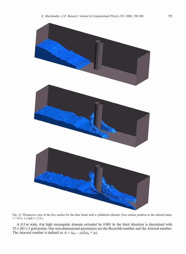
Fig. 15. Perspective view of the free surface for the dam break with a cylindrical obstacle. Free surface position at the selected times:t = 0.5 s, 1 s and t = 2.5 s.
E. Marchandise, J.-F. Remacle / Journal of Computational Physics 219 (2006) 780–800 795
A 0.5 m wide, 4 m high rectangular domain extruded by 0.001 in the third direction is discretized with32 · 265 · 2 grid points. Our non-dimensional parameters are the Reynolds number and the Atwood number.The Atwood number is defined as A = (qh � ql)/(qh + ql).
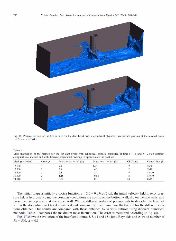
Fig. 16. Perspective view of the free surface for the dam break with a cylindrical obstacle. Free surface position at the selected times:t = 2 s and t = 2.64 s.
Table 2Mass fluctuation of the method for the 3D dam break with cylindrical obstacle computed at time t = 1 s and t = 2 s on differentcomputational meshes and with different polynomial orders p to approximate the level set
Mesh (nb nodes) Order p Mass loss (t = 1 s) (%) Mass loss (t = 2 s) (%) CPU (nb) Comp. time (h)
12.500 1 7.4 14.3 2 1h3012.500 2 3.4 6.2 2 3h1012.500 3 2.1 3.1 4 15h1030.820 2 1.16 0.86 8 13h1074.016 2 0.62 0.11 24 6h45
796 E. Marchandise, J.-F. Remacle / Journal of Computational Physics 219 (2006) 780–800
The initial shape is initially a cosine function z = 2.0 + 0.05cos(2px), the initial velocity field is zero, pres-sure field is hydrostatic, and the boundary conditions are no-slip on the bottom wall, slip on the side walls, andprescribed zero pressure at the upper wall. We use different orders of polynomials to describe the level setwithin the discontinuous Galerkin method and compare the maximum mass fluctuation for the different solu-tions obtained. Our results are compared with those obtained by various authors using different numericalmethods. Table 3 compares the maximum mass fluctuation. The error is measured according to Eq. (8).
Fig. 17 shows the evolution of the interface at times 5, 8, 11 and 15 s for a Reynolds and Atwood number ofRe = 500, A = 0.5.
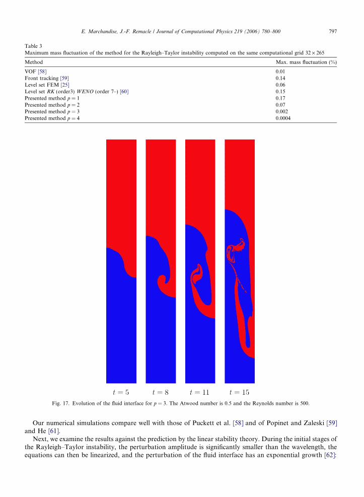
Fig. 17. Evolution of the fluid interface for p = 3. The Atwood number is 0.5 and the Reynolds number is 500.
Table 3Maximum mass fluctuation of the method for the Rayleigh–Taylor instability computed on the same computational grid 32 · 265
Method Max. mass fluctuation (%)
VOF [58] 0.01Front tracking [59] 0.14Level set FEM [25] 0.06Level set RK (order3) WENO (order 7–) [60] 0.15Presented method p = 1 0.17Presented method p = 2 0.07Presented method p = 3 0.002Presented method p = 4 0.0004
E. Marchandise, J.-F. Remacle / Journal of Computational Physics 219 (2006) 780–800 797
Our numerical simulations compare well with those of Puckett et al. [58] and of Popinet and Zaleski [59]and He [61].
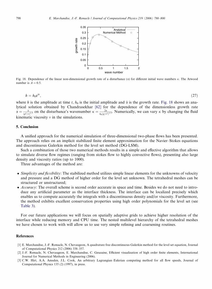
Next, we examine the results against the prediction by the linear stability theory. During the initial stages ofthe Rayleigh–Taylor instability, the perturbation amplitude is significantly smaller than the wavelength, theequations can then be linearized, and the perturbation of the fluid interface has an exponential growth [62]:
0
0.05
0.1
0.15
0.2
0.25
0.3
0.35
0 0.5 1 1.5 2
grow
th r
ate
wave number
AnalyticalNumerical Method
Fig. 18. Dependence of the linear non-dimensional growth rate of a disturbance (a) for different initial wave numbers j. The Atwoodnumber is A = 0.5.
798 E. Marchandise, J.-F. Remacle / Journal of Computational Physics 219 (2006) 780–800
h ¼ h0eat; ð27Þ
where h is the amplitude at time t, h0 is the initial amplitude and a is the growth rate. Fig. 18 shows an ana-lytical solution obtained by Chandrasekhar [62] for the dependence of the dimensionless growth ratea ¼ aðg2=mÞ1=3 on the disturbance’s wavenumber j ¼ 2ph0ðg=m2Þ1=3. Numerically, we can vary j by changing the fluid
kinematic viscosity m in the simulations.
5. Conclusion
A unified approach for the numerical simulation of three-dimensional two-phase flows has been presented.The approach relies on an implicit stabilized finite element approximation for the Navier–Stokes equationsand discontinuous Galerkin method for the level set method (DG-LSM).
Such a combination of those two numerical methods results in a simple and effective algorithm that allowsto simulate diverse flow regimes (ranging from stokes flow to highly convective flows), presenting also largedensity and viscosity ratios (up to 1000).
Three advantages of the method are:
� Simplicity and flexibility: The stabilized method utilizes simple linear elements for the unknowns of velocityand pressure and a DG method of higher order for the level set unknown. The tetrahedral meshes can bestructured or unstructured;� Accuracy: The overall scheme is second order accurate in space and time. Besides we do not need to intro-
duce any artificial parameter as the interface thickness. The interface can be localized precisely whichenables us to compute accurately the integrals with a discontinuous density and/or viscosity. Furthermore,the method exhibits excellent conservation properties using high order polynomials for the level set (seeTable 3).
For our future applications we will focus on spatially adaptive grids to achieve higher resolution of theinterface while reducing memory and CPU time. The nested multilevel hierarchy of the tetrahedral mesheswe have chosen to work with will allow us to use very simple refining and coarsening routines.
References
[1] E. Marchandise, J.-F. Remacle, N. Chevaugeon, A quadrature free discontinuous Galerkin method for the level set equation, Journalof Computational Physics 212 (2006) 338–357.
[2] J.-F. Remacle, N. Chevaugeon, E. Marchandise, C. Geuzaine, Efficient visualization of high order finite elements, InternationalJournal for Numerical Methods in Engineering (2006).
[3] C.W. Hirt, A.A. Amsden, J.L. Cook, An arbitrary Lagrangian–Eulerian computing method for all flow speeds, Journal ofComputational Physics 135 (2) (1997), in press.
E. Marchandise, J.-F. Remacle / Journal of Computational Physics 219 (2006) 780–800 799
[4] T. Hughes, W. Liu, T. Zimmermann, Lagrangian–Eulerian finite element formulation for incompressible viscous flows, ComputerMethods in Applied Mechanics and Engineering 29 (1981) 239–349.
[5] J. Donea, Arbitrary Lagrangian–Eulerian finite element methods, Computational Methods for Transient Analysis 1 (1983) 473–516.[6] W. Dettmer, P. Saksono, D. Peric, On a finite element formulation for incompressible Newtonian fluid flows on moving domains in
the presence of surface tension, Computer Methods in Applied Mechanics and Engineering 19 (2003) 659–668.[7] F. Harlow, J. Welch, Volume tracking methods for interfacial flow calculations, Physics of Fluids 8 (1965) 21–82.[8] C. Hirt, B. Nichols, Volume of fluid method (VOF) for the dynamics of free boundaries, Journal of Computational Physics 39 (1981)
201–225.[9] J. Pilliot, E. Puckett, Second order accurate volume-of-fluid algorithms for tracking material interfaces, Journal of Computational
Physics 199 (2004) 465–502.[10] S. Osher, J.A. Sethian, Fronts propagating with curvature dependent speed: algorithms based on Hamilton–Jacobi formulations,
Journal of Computational Physics 79 (1988) 12–49.[11] M. Sussman, E. Fatemi, An efficient interface preserving level set redistancing algorithm and its application to interfacial
incompressible fluid flow, SIAM Journal on Scientific Computing 20 (1999) 1165–1191.[12] M. Sussman, P. Smereka, S. Osher, A level set approach for computing solutions to incompressible two-phase flow, Journal of
Computational Physics 114 (1994) 146–159.[13] M. Sussman, E. Fatemi, P. Smereka, S. Osher, An improved level set method for incompressible two-fluid flows, Computers and
Fluids 27 (1998) 663–680.[14] J. Chessa, T. Belytschko, An extended finite element method for two-phase fluids, Journal of Applied Mechanics (Transactions of the
ASME) 70 (2003) 10–17.[15] J. Chessa, T. Belytschko, An enriched finite element method and level sets for axisymmetric two-phase flow with surface tension,
International Journal for Numerical Methods in Engineering 58 (2003) 2041–2064.[16] C. Norman, M. Miksis, Non-linear dynamics of thin films and fluid interfaces, Physica D: Nonlinear Phenomena 209 (2005) 191–204.[17] S. Nagrath, K. Jansen, R. Lahey, Computation of incompressible bubble dynamics with a stabilized finite element level set method,
Computer Methods in Applied Mechanics and Engineering 194 (42–44) (2005) 4565–4587.[18] S. Osher, C.-W. Shu, High order essentially non-oscillatory schemes for Hamilton–Jacobi equations, SIAM Journal on Numerical
Analysis 728 (1991) 902–921.[19] C. Hu, C.-W. Shu, Weighted ENO schemes for Hamilton–Jacobi equations, SIAM Journal on Scientific Computing 21 (6) (1999)
2126–2143.[20] D. Enright, R. Fedkiw, J. Ferziger, I. Mitchell, A hybrid particle level set method for improved interface capturing, Journal of
Computational Physics 183 (2002) 83–116.[21] S. Nagrath, K. Jansen, R. Lahey, Computation of incompressible bubble dynamics with a stabilized finite element level set method,
Computer Methods in Applied Mechanics and Engineering 194 (2005) 4565–4587.[22] A.-K. Tornberg, B. Engquist, A finite element based level set method for multiphase flow applications, Computing Visualization in
Science 3 (2000) 93–101.[23] S. van der Pijl, A. Segal, C. Vuik, P. Wesseling, A mass-conserving levelset method for modeling of multiphase flows, International
Journal for Numerical Methods in Fluids 47 (2004) 339–361.[24] J. Ferziger, Interfacial transfer in Tryggvason’s method, International Journal for Numerical Methods in Fluids 41 (5) (2003) 551–560.[25] A. Smoliansky, Numerical modeling of two-fluid interfacial flows, Ph.D. Thesis, University of Jyvaskyla, Finland, 2001.[26] A.-K. Tornberg, Interface tracking methods with applications to multiphase flows, Ph.D. Thesis, Royal Institute of Technology
(KTH), Finland, 2000.[27] A. Chorin, Numerical solution of the Navier–Stokes equations, Mathematical Computation 22 (1968) 745–762.[28] Y. Kallinderis, K. Nakajima, Finite element method for incompressible viscous flow with adaptative grids, AIAA Journal 8 (32)
(1994), in press.[29] Y. Kallinderis, W. Schulz, Unsteady flow structure interaction for incompressible flows using deformable grids, Journal of
Computational Physics 143 (2) (1998) 569–597.[30] T.J.R. Hughes, L.P. Franca, A new finite element formulation for computational fluid dynamics: V. circumventing the Babuska–
Brezzi condition: A stable Petrov–Galerkin formulation of the stokes problem accommodating equal-order interpolations, ComputerMethods in Applied Mechanics and Engineering 59 (1986) 85–99.
[31] T. De Mulder, Stabilized finite elements methods for turbulent incompressible single-phase and dispersed two-phase flows, Ph.D.Thesis, von Karman Institute For Fluid Dynamics, Belgium, 1997.
[32] A. Chorin, A numerical method for solving incompressible viscous flow problems, Journal of Computational Physics 135 (2) (1997)118–125.
[33] S. Rogers, D. Kwak, C. Kiris, Steady and unsteady solutions of the incompressible Navier–Stokes equations, AIAA Journal 29 (1991)306–610.
[34] T. Hughes, L. Franca, G. Hulbert, A new finite element formulation for fluid dynamics: VIII. The Galerkin/least-squares method foradvective–diffusive equations, Computer Methods in Applied Mechanics and Engineering 73 (1989) 173–189.
[35] L. Franca, S. Frey, Stabilized finite element methods: II. The incompressible Navier Stokes equations, Computer Methods in AppliedMechanics and Engineering 59 (1992) 209–233.
[36] O. Ladyshenskaya, The Mathematical Theory of Viscous Incompressible Flow, Gordon and Breach, New York, 1969.[37] I. Babuska, The finite element method with Lagrangian multipliers, Numerical Mathematics 179 (1971), in press.[38] F. Brezzi, M. Fortin, Mixed and Hybrid Finite Element Methods, Springer, New York, 1991.
800 E. Marchandise, J.-F. Remacle / Journal of Computational Physics 219 (2006) 780–800
[39] J.-F. Remacle, J. Flaherty, M. Shephard, An adaptive discontinuous Galerkin technique with an orthogonal basis applied tocompressible flow problems, SIAM Review 45 (2003) 53–72.
[40] J.-F. Remacle, M.S. Shephard, An algorithm oriented mesh database, International Journal for Numerical Methods in Engineering58 (2) (2003) 349–374.
[41] I. Babuska, The finite element method with Lagrangian multipliers, Numerische Mathematik 20 (1971) 179–192.[42] F. Brezzi, On the existence uniqueness and approximation of saddle-point problems arising from Lagrange multipliers, R.A.I.R.O.,
Serie Rouge Analyse Numerique 8 (1974) 129–151.[43] T. Tezduyar, Y. Osawa, Finite element stabilization parameters computed from element matrices and vectors, Computer Methods in
Applied Mechanics and Engineering 190 (2000) 411–430.[44] F. Shakib, T. Hughes, Z. Johan, A new finite element formulation for computational fluid dynamics: the compressible Euler and
Navier–Stokes equations, Computer Methods in Applied Mechanics and Engineering 89 (1991) 141–219.[45] T.J. Barth, Aspects of unstructured grids and finite-volume solvers for the Euler and Navier–Stokes equations, Special course on
unstructured grid methods for advection dominated flows, AGARD R-787, 1992 (Chapter 4).[46] V. Selmin, L. Formaggia, Unified construction of finite element and finite volume discretizations for compressible flows, International
Journal for Numerical Methods in Fluids 39 (1996) 1–32.[47] P. Geuzaine, An implicit upwind finite volume method for compressible turbulent flows on unstructured meshes, Ph.D. Thesis,
Universite de Liege, Belgium, 1999.[48] M. Mount, N.S. Arya, R. Netanyahu, Silverman, An optimal algorithm for approximate nearest neighbor searching, Journal of the
ACM 45 (1998), in press.[49] ANN library. Available from: URL <http://www.cs.umd.edu/~mount/ANN/>.[50] P. Geuzaine, Newton–Krylov strategy for compressible turbulent flows on unstructured meshes, AIAA Journal 39 (2001) 528–531.[51] X.C. Cai, C. Farhat, M. Sarkis, A minimum overlap restricted additive Schwarz preconditioner and applications in 3D flow
simulations, Contemporary Mathematics 218 (1998) 478–484.[52] A. Prosperetti, Motion of two superimposed viscous fluids, Physics of Fluids 24 (1981) 1217–1223.[53] G. Wu, R. Eatock Taylor, D. Greaves, The effect of viscosity on the transient free-surface waves in a two-dimensional tank, Journal of
Engineering Mathematics 40 (2001) 77–90.[54] J. Martin, W. Moyce, An experimental study of the collapse of liquid columns on a rigid horizontal plane, Philosophical Transactions
A 244 (1952) 312–324.[55] A. Ritter, Die fortpflanzung der wasserwellen., Z. Ver. deut. Ing. 36 (1982), in press.[56] M. Quecedo, M. Pastor, M. Herreros, Comparison of two mathematical models for solving the dam break problem using the FEM
method, Computer Methods in Applied Mechanics and Engineering (in press).[57] T. Shigematsu, P. Liu, K. Oda, Numerical modeling of the initial stages of dam-break waves, Journal of Hydraulic Research 42 (2)
(2004) 183–195.[58] E. Puckett, A. Almgren, J. Bell, D. Marcus, W. Rider, A high-order projection method for tracking fluid interfaces in variable density
incompressible flows, Journal of Computational Physics 130 (1997) 269–282.[59] S. Popinet, S. Zaleski, A front-tracking algorithm for accurate representation of surface tension, International Journal for Numerical
Methods in Fluids 30 (1999) 775–793.[60] R.R. Nourgaliev, T.N. Dinh, T.G. Theofanous, A pseudocompressibility method for the numerical simulation of incompressible
multifluid flows, International Journal of Multiphase Flow 30 (2004) 6001–6937.[61] M. Mount, N.S. Arya, R. Netanyahu, Silverman, A lattice Boltzmann scheme for incompressible multiphase flow and its application
in simulation of Rayleigh, Journal of Computational Physics 152 (2) (1999) 642–663.[62] S. Chandrasekhar, Hydrodynamic and Hydromagnetic Stability, Clarendon Press, Oxford, 1961.
Related Documents