A stabilised Petrov–Galerkin formulation for linear tetrahedral elements in compressible, nearly incompressible and truly incompressible fast dynamics Antonio J. Gil ⇑ , Chun Hean Lee, Javier Bonet, Miquel Aguirre Zienkiewicz Centre for Computational Engineering, College of Engineering Swansea University, Singleton Park SA2 8PP, United Kingdom Received 18 December 2013; received in revised form 7 April 2014; accepted 13 April 2014 Available online 26 April 2014 Abstract A mixed second order stabilised Petrov–Galerkin finite element framework was recently introduced by the authors (Lee et al., 2014) [46]. The new mixed formulation, written as a system of conservation laws for the linear momentum and the deformation gradient, performs extremely well in bending dominated scenarios (even when linear tetrahedral elements are used) yielding equal order of convergence for displacements and stresses. In this paper, this formulation is further enhanced for nearly and truly incompressible deformations with three key novelties. First, a new conservation law for the Jacobian of the deformation is added into the system providing extra flexibility to the scheme. Second, a variationally consistent Petrov–Galerkin stabilisation methodology is derived. Third, an adapted fractional step method is presented for both incompressible and nearly incompressible materials in the context of nonlinear elastodynamics. For completeness and ease of understanding, these three improvements are presented both in small and large strain regimes, studying the eigen- structure of the resulting systems. A series of numerical examples are presented in order to demonstrate the robustness of the enhanced methodology with respect to the work previously published by the authors. Ó 2014 Elsevier B.V. All rights reserved. Keywords: Fast dynamics; Petrov–Galerkin; Fractional step; Incompressible; Locking; Geometric conservation law 1. Introduction Classical displacement-based finite element formulations [1–7] are typically employed in industry when simulating complex engineering problems. For these applications, linear tetrahedral elements tend to be preferred when dealing with complex three dimensional geometries, due to the maturity of the existing unstructured mesh generators. However, this methodology presents a number of well-known shortcomings. http://dx.doi.org/10.1016/j.cma.2014.04.006 0045-7825/Ó 2014 Elsevier B.V. All rights reserved. ⇑ Corresponding author. Tel.: +44 (0) 1792602552. E-mail address: [email protected] (A.J. Gil). Available online at www.sciencedirect.com ScienceDirect Comput. Methods Appl. Mech. Engrg. 276 (2014) 659–690 www.elsevier.com/locate/cma

Welcome message from author
This document is posted to help you gain knowledge. Please leave a comment to let me know what you think about it! Share it to your friends and learn new things together.
Transcript
Available online at www.sciencedirect.com
ScienceDirect
Comput. Methods Appl. Mech. Engrg. 276 (2014) 659–690
www.elsevier.com/locate/cma
A stabilised Petrov–Galerkin formulation for lineartetrahedral elements in compressible, nearly incompressible
and truly incompressible fast dynamics
Antonio J. Gil ⇑, Chun Hean Lee, Javier Bonet, Miquel Aguirre
Zienkiewicz Centre for Computational Engineering, College of Engineering Swansea University, Singleton Park SA2 8PP, United Kingdom
Received 18 December 2013; received in revised form 7 April 2014; accepted 13 April 2014Available online 26 April 2014
Abstract
A mixed second order stabilised Petrov–Galerkin finite element framework was recently introduced by the authors (Leeet al., 2014) [46]. The new mixed formulation, written as a system of conservation laws for the linear momentum and thedeformation gradient, performs extremely well in bending dominated scenarios (even when linear tetrahedral elements areused) yielding equal order of convergence for displacements and stresses. In this paper, this formulation is furtherenhanced for nearly and truly incompressible deformations with three key novelties. First, a new conservation law forthe Jacobian of the deformation is added into the system providing extra flexibility to the scheme. Second, a variationallyconsistent Petrov–Galerkin stabilisation methodology is derived. Third, an adapted fractional step method is presented forboth incompressible and nearly incompressible materials in the context of nonlinear elastodynamics. For completeness andease of understanding, these three improvements are presented both in small and large strain regimes, studying the eigen-structure of the resulting systems. A series of numerical examples are presented in order to demonstrate the robustness ofthe enhanced methodology with respect to the work previously published by the authors.� 2014 Elsevier B.V. All rights reserved.
Keywords: Fast dynamics; Petrov–Galerkin; Fractional step; Incompressible; Locking; Geometric conservation law
1. Introduction
Classical displacement-based finite element formulations [1–7] are typically employed in industry whensimulating complex engineering problems. For these applications, linear tetrahedral elements tend to bepreferred when dealing with complex three dimensional geometries, due to the maturity of the existingunstructured mesh generators. However, this methodology presents a number of well-known shortcomings.
http://dx.doi.org/10.1016/j.cma.2014.04.006
0045-7825/� 2014 Elsevier B.V. All rights reserved.
⇑ Corresponding author. Tel.: +44 (0) 1792602552.E-mail address: [email protected] (A.J. Gil).
660 A.J. Gil et al. / Comput. Methods Appl. Mech. Engrg. 276 (2014) 659–690
First, reduced order of convergence for derived variables (i.e. second order for displacements but first orderfor stresses), requiring some form of stress recovery procedure if these are of interest [8,9]. Second, the perfor-mance of these formulations in bending dominated scenarios can be very poor [10,11] yielding unacceptableresults. Third, the presence of numerical instabilities in the form of volumetric locking, shear locking andspurious hydrostatic pressure fluctuations [12,13] when large Poisson’s ratios are used. This aspect is partic-ularly relevant in the context of biomedical modelling. Fourth, from the time discretisation point of view,Newmark-type methods [14] have a tendency to introduce high frequency noise, especially in the vicinity ofsharp spatial gradients and accuracy is degraded once numerical artificial damping is employed [15–19]. Theseschemes are thus not desirable for shock dominated problems.
Significant efforts have been undertaken to develop effective linear tetrahedral formulations for nearlyincompressible solids. Multi-field Fraeijs de Veubeke–Hu–Washizu (FdVHW) type variational principles[20] are among them, where independent kinematic descriptions are used for the volumetric and deviatoriccomponents of the deformation. The conventional mean dilatation method [21] is a particular case of SelectiveReduced Integration, where the volumetric deformation is suitably underintegrated [15]. Unfortunately, themean dilatation approach cannot be employed with linear tetrahedrals and authors resort to some form ofprojection to reduce the number of volumetric constraints [21–29]. Alternatively, high order interpolationapproaches can be used [30,31]. However, the increase in the number of integration points can drasticallyreduce the computational efficiency of these schemes in comparison with low order approaches, specially whencomplex constitutive laws must be modelled (e.g. visco-elasticity, visco-plasticity).
A family of nodally integrated tetrahedral elements was formulated in [32], where the volumetric strainenergy functional was approximated through averaged nodal pressures. However, the resulting approachwas reported to behave poorly in bending dominated scenarios. To overcome this difficulty, reference [11] pro-posed the nodal based uniform strain tetrahedral element by applying a nodal averaging process to the wholesmall strain tensor. Reference [33] extended this application to the large strain regime with the idea of employ-ing both a nodal average Jacobian and a nodal average deformation gradient in the calculation of the stresstensor. As reported in [34–37], the resulting formulation suffers from artificial mechanisms similar to hourgl-assing unless some form of stabilisation is used. Despite exhibiting very good behaviour in terms of displace-ments, this class of averaged nodal strain tetrahedral formulations tend to exhibit non-physical hydrostaticpressure fluctuations [34,38].
In parallel, in reference [39], a stabilised Petrov–Galerkin (PG) formulation by using the Galerkin LeastSquares (GLS) approach is first introduced for the analysis of the Stokes problem, with equal order of inter-polation for velocity and pressure. The formulation circumvents the Ladyzenskaya–Babuska–Brezzi (LBB)condition [40,41], ensuring numerical stability and optimal convergence.
At present and to the best of our knowledge, most of the proposed schemes for linear tetrahedral elementsare restricted to elastostatics [34,42–45]. The development of an effective linear tetrahedral formulation in therange of fully and nearly incompressible large strain dynamics remains an open issue.
The aim of this paper is to improve the robustness and effectiveness of the stabilised Petrov–Galerkin (PG)mixed finite element framework recently presented in [46], extending its applicability to the range of fully andnearly incompressible materials. This mixed methodology is formulated in the form of a system of first orderconservation laws [10,46–48], where the linear momentum p and the deformation gradient tensor F of the sys-tem are regarded as the main conservation variables of this mixed p-F approach. In [46], a robust and stablePG implementation is presented, derived with the help of the Variational Multi-Scale (VMS) method [49–52].Unfortunately, in the case of extreme deformations in the incompressible limit (i.e. refer to twisting columnexample in Section 4.4 of this paper), the p-F formulation lacks robustness.
With this in mind, this mixed PG formulation is first enhanced by introducing a new conservation law forthe Jacobian J of the deformation (volumetric strain in the small strain regime), also known as a GeometricConservation Law [53]. The volumetric stress component appearing in the conservation of linear momentumequation is then evaluated from this new conservation law, providing more flexibility and robustness to thescheme.
For computational efficiency, the enhanced p-F-J formulation is implemented in conjunction with an expli-cit time integrator, where the time step size is controlled through the Courant–Friedrichs–Lewy number [54]by the volumetric wave speed cp. In the incompressibility limit, cp can reach very high values leading to a very
A.J. Gil et al. / Comput. Methods Appl. Mech. Engrg. 276 (2014) 659–690 661
inefficient algorithm. Moreover, in the case of full incompressibility, the explicit p-F-J formulation cannot beused.
In order to address this issue, we then present an alternative adapted variationally consistent fractional step[55–57] PG formulation. This fractional step approach is very typical in the context of Computational FluidDynamics for incompressible flows [58,59] and has been already used in the context of large deformation soliddynamics [60]. In this case, the allowable time step is found to depend only on the shear wave speed cs,circumventing the volumetric wave speed constraint.
The outline of the present paper is as follows. In Section 2 we start by introducing the enhanced stabilisedPG formulation for linear elastodynamics. Governing equations, eigenstructure of the problem and the PGstabilisation are presented. For incompressible or nearly incompressible materials, an alternative fractionalstep approach is also presented. We then extend these formulations to nonlinear large strain elastodynamics(see Section 3). The governing conservation laws are particularised for the case of a nearly incompressibleNeo–Hookean material and the eigenstructure of the problem is studied in detail in order to demonstratethe rank-one convexity requirement [61]. This section ends with the PG stabilisation procedure as well asthe alternative fractional step approach. In Section 4, a series of numerical examples are presented to assessthe robustness of the enhanced formulations and to draw some comparisons against previous results publishedby the authors [46]. Finally, Section 5 presents some concluding remarks and current directions of research.
2. Linear reversible elastodynamics
2.1. Enhanced p-G-j mixed methodology
In the context of small deformations, let us consider the motion of a continuum defined by a domain v � R3
of boundary @v with outward unit normal n. This motion is defined by a displacement field u ¼ uðx; tÞ where xrepresents a material point and t the time. Let us also introduce the following scalar, vector and second ordertensor variables: q is the density of the continuum, p is the linear momentum, G is the displacement gradienttensor, j is the volumetric strain, r is the (symmetric) Cauchy stress tensor, b is a body force per unit of massand ET denotes the total energy per unit of volume. It is then possible to describe the motion of the continuumby means of a system of first order conservation laws as follows
1 $ i
@p
@t� divr ¼ qb; ð1aÞ
@G
@t� div
1
qp� I
� �¼ 0; ð1bÞ
@j@t� div
p
q
� �¼ 0; ð1cÞ
@ET
@t� div
1
qrT p�Q
� �¼ s: ð1dÞ
In above system (1a)–(1d), div is the divergence operator defined by the tensor contraction of the last indexand I is the identity tensor with Kronecker delta components ½I �ij ¼ dij. Eq. (1a) represents the conservationof linear momentum, (1b) and (1c) represent evolution equations for the displacement gradient tensor and thevolumetric strain, respectively, and Eq. (1d) denotes the conservation of the total energy per unit of volume.
In the case of an adiabatic deformation, the heat flux Q and the heat source s are neglected. In addition, fora non-thermomechanical material Eq. (1d) is fully decoupled from the rest of the system. From thecomputational point of view, this equation is still very useful when evaluating the numerical diffusion(entropy) introduced by the algorithm. The Cauchy stress tensor r is considered a function of G and j, whichare evaluated through Eqs. (1b) and (1c), respectively. In other words, in this mixed formulation, G and j arenot explicitly evaluated through the displacement field, namely $u and divu, respectively.1 This enhanced
s the spatial gradient operator.
662 A.J. Gil et al. / Comput. Methods Appl. Mech. Engrg. 276 (2014) 659–690
p-G-j mixed methodology will render great benefits when dealing with bending dominated nearly or trulyincompressible deformations.
Finally, the above system (1a)–(1c) of conservation laws can be written in a more compact form as
2 Ein
@U
@tþ @F i
@xi¼ S; i ¼ 1; 2; 3; ð2Þ
where U represents the vector of conservation variables, F i is the flux vector in the spatial direction i and S isa source term.2 The components of U;F i and S can be vectorised leading to 13� 1 column vectors as
U ¼
p1
p2
p3
G11
G12
G13
G21
G22
G23
G31
G32
G33
j
2666666666666666666666666664
3777777777777777777777777775
; F i ¼
�r1i
�r2i
�r3i
�di1v1
�di2v1
�di3v1
�di1v2
�di2v2
�di3v2
�di1v3
�di2v3
�di3v3
�vi
2666666666666666666666666664
3777777777777777777777777775
; S ¼
qb1
qb2
qb3
0
0
0
0
0
0
0
0
0
0
2666666666666666666666666664
3777777777777777777777777775
: ð3Þ
For clarity, individual conservations laws will be used for each component of the vector of conservationvariables U as
U ¼p
G
j
264
375; F n ¼ F ini ¼
�rn
� 1q p� n
� 1q p � n
264
375; S ¼
qb
0
0
264
375: ð4Þ
For the closure of the above system (1a)–(1c), a constitutive law is required relating r and G and j. In this case,we employ a linear elastic isotropic constitutive law of the form
r ¼ l G þ GT � 2
3trGð ÞI
� �|fflfflfflfflfflfflfflfflfflfflfflfflfflfflfflfflfflfflfflffl{zfflfflfflfflfflfflfflfflfflfflfflfflfflfflfflfflfflfflfflffl}
rdev
þ pI|{z}rvol
; p ¼ jj; ð5Þ
where rdev and rvol represent the deviatoric and volumetric components of the Cauchy stress, p is the hydro-static pressure and l and j are the shear and bulk moduli, respectively. Above system (2) can be re-written inquasi-linear format
@U
@tþA i
@U
@xi¼ S; i ¼ 1; 2; 3; ð6Þ
where the corresponding flux Jacobian matrix An ¼ A ini is evaluated as
stein’s summation will be implied for repeated indices unless otherwise explicitly stated.
A.J. Gil et al. / Comput. Methods Appl. Mech. Engrg. 276 (2014) 659–690 663
An ¼
� @ rnð Þ@p
� @ rnð Þ@G
� @ rnð Þ@j
� @ 1qp�nð Þ@p
� @ 1qp�nð Þ@G
� @ 1qp�nð Þ@j
� @ 1qp�nð Þ@p
� @ 1qp�nð Þ@G
� @ 1qp�nð Þ@j
266664
377775 ¼
03�3 �cdevn �jn
� 1q In 03�3�3�3 03�3�1
� 1q n 03�3 0
264
375; ð7Þ
where
½cdevn �ijk ¼ ½c
dev�iljknl ¼@½rdev�il@½G �jk
nl ¼ l dijnk þ diknj �2
3djkni
� �; ð8aÞ
½In�ijk ¼ diknj: ð8bÞ
For completeness, the residuals R ¼ ½Rp;RG ;Rj�T of the balance principles (1a)–(1c) can be defined as
Rp :¼ div rþ qb� _p; ð9aÞ
RG :¼ $p
q
� �� _G; ð9bÞ
Rj :¼ divp
q
� �� _j; ð9cÞ
where ð _: Þ indicates derivative with respect to time. These residuals will be used later in the paper when derivinga stabilised formulation.
2.2. Eigenvalue structure
The study of the eigenvalue structure of the system is important to guarantee its hyperbolicity. Theeigenvalues and eigenvectors of system (6) can be evaluated considering plane wave solutions of the form
U ¼ /ðx � n� catÞUa ¼ /ðx � n� catÞpa
Ga
ja
264
375; ð10Þ
where ca are the eigenvalues (wave speeds) corresponding to the eigenvector Ua. Substitution of expression(10) into system (6) renders
caUa ¼ AnUa: ð11Þ
The above system (11) can be expanded as
capa ¼ �cdevn Ga � jjan; ð12aÞ
caGa ¼�1
qpa � n; ð12bÞ
caja ¼�1
qpa � n: ð12cÞ
Substitution of Eqs. (12b) and (12c) into (12a) and after making use of (8a), it renders
qc2apa ¼
4
3lþ j
� �n� nþ lðI � n� nÞ
� �pa; ð13Þ
where it can be seen that the system contains three pairs of non-zero eigenvalues corresponding to thevolumetric and shear waves as
c1;2 ¼ �cp; cp ¼
ffiffiffiffiffiffiffiffiffiffiffiffiffiffi43lþ j
q
s; c3;4 ¼ c5;6 ¼ �cs; cs ¼
ffiffiffilq
r; ð14Þ
664 A.J. Gil et al. / Comput. Methods Appl. Mech. Engrg. 276 (2014) 659–690
with eigenvectors
U1;2 ¼n
� 1qcp
n� n
� 1qcp
2664
3775; U3;4 ¼
t1
� 1qcs
t1 � n
0
264
375; U5;6 ¼
t2
� 1qcs
t2 � n
0
264
375: ð15Þ
where t1 and t2 are two arbitrary tangential vectors orthogonal to n. The rest of the eigenvalues are zero andhave null associated velocity components. As can be observed, both volumetric and shear waves always takereal values, ensuring the hyperbolicity of the system.
For a fully incompressible material, the conservation equation for the volumetric strain (1c) is replaced by
the constraint div pq
� ¼ 0 and thus, Eq. (12c) gets replaced by the constraint pa � n ¼ 0. This constraint, once
substituted into Eq. (13) yields
qc2apa ¼ lpa; ð16Þ
leading to only two pairs of non-zero eigenvalues corresponding to the shear waves c3;4 ¼ c5;6 ¼ �cs with
eigenvectors U3;4 and U5;6.
2.3. Linearised Petrov–Galerkin formulation
A stabilised Petrov–Galerkin (PG) framework incorporating suitable numerical diffusion into the standardBubnov–Galerkin formulation is presented next. First, we derive a single variational statement that satisfiesthe second law of thermodynamics [62,63] through the use of work-conjugate principles [64]. Multiplication
of the residuals R ¼ ½Rp;RG ;Rj�T with a set of appropriate conjugate virtual fields dVst ¼ ½dvst; drst; dqst�Tand integration over the domain v gives
dW PGðU; dVstÞ ¼Z
vdvst �Rp dvþ
Zv
drst : RG dvþZ
vdqstRj dv ¼ 0: ð17Þ
Note that dvst is the stabilised virtual velocity, drst is the stabilised virtual Cauchy stress and dqst is the stabi-lised virtual pressure. Pairs such as fdvst;Rpg; fdrst;RGg and fdqst;Rjg are said to be dual or work conjugatewith respect to the volume v in the sense that their inner product yields work rate per unit of volume.
Following the Streamline Upwind Petrov–Galerkin (SUPG) [65–69] approach, stabilised virtual fields canbe defined as
dVst ¼ dV þ sTATi
@dV@xi
; ð18Þ
where s is the matrix of stabilisation parameters. We can now particularise the above expression (18) to the setof conjugate virtual fields of interest in this paper as
dvst ¼ dv� spG
qdivdr� spj
q$dq; ð19aÞ
drst ¼ dr� sGp cdev : $dv; ð19bÞ
dqst ¼ dq� sjp j divdv; ð19cÞ
where cdev is the tangent deviatoric constitutive tensor (8a) and spG , spj; sGp and sjp are appropriate stabilisa-tion parameters. Substitution of Eqs. (19a)–(19c) into (17) yields
dW PGdv ðU; dvÞ ¼
Zv
dv �Rp � sGp$dv : cdev : RG � sjp j ðdivdvÞRj
�dv ¼ 0; ð20aÞ
dW PGdr ðU; drÞ ¼
Zv
dr : RG �spG
qðdivdrÞ �Rp
� �dv ¼ 0; ð20bÞ
A.J. Gil et al. / Comput. Methods Appl. Mech. Engrg. 276 (2014) 659–690 665
dW PGdq ðU; dqÞ ¼
Zv
dqRj �spj
qð$dqÞ �Rp
� �dv ¼ 0: ð20cÞ
Following a standard finite element isoparametric methodology [64], the conservation variables U as well asthe virtual fields dV can be discretised in terms of nodal values (Ua; dVa) and suitable shape functions Na,where a ¼ f1; . . . ; ng; n being the total number of nodes of the underlying mesh. In our case, linear shape func-tions are preferred guaranteeing thus second order convergence. It is easier to first consider the discretisedweak statement of the linear momentum balance principle dW PG
dv (20a). Given the interpolation of the virtualvelocity dv ¼
PaN adva and the arbitrariness of dva, it yields
ZvNaq _v dv ¼
Z@v
NatB daþZ
vN aqb dv�
Zv½rdev þ sGpcdev : RG �|fflfflfflfflfflfflfflfflfflfflfflfflfflfflfflffl{zfflfflfflfflfflfflfflfflfflfflfflfflfflfflfflffl}
rdev;st
$Na dv�Z
v½p þ jsjpRj�|fflfflfflfflfflfflfflffl{zfflfflfflfflfflfflfflffl}
pst
$N a dv; ð21Þ
where tB is the boundary traction vector defined as rn (obtained from appropriate boundary conditions).Observe that the squared bracket terms on the right-hand side of (21) describe the stabilised deviatoric Cauchystress rdev;st and the stabilised pressure pst. More generally, these stabilised kinetic fields rdev;st and pst can bereinterpreted by using the Variational Multi-Scale (VMS) method [49–52,70–73] as
rdev;st :¼ rdevðG stÞ; pst :¼ pðjstÞ; ð22Þ
where the stabilised displacement gradient G st and volumetric strain jst are defined as
G st :¼ G þ sGpRG; ð23aÞjst :¼ jþ sjpRj: ð23bÞ
Substitution of Eqs. (22), (23a), and (23b) into (21) and after expanding _p ¼P
bN b _pb, results in
XbMab _pb ¼Z@v
N atB daþZ
vNaqb dv�
Zv
rðG st; jstÞ$Na dv; ð24Þ
where Mab ¼MabI with Mab ¼R
v NaNb dv �
the consistent mass contribution. An identical spatial discreti-
sation procedure can now be followed for dW PGdr (20b) and dW PG
dq (20c) by employing similar finite element
expansions fdr ¼P
aN adra; dq ¼P
aN adqag and f _G ¼P
bN b_Gb; _j ¼
PbNb _jbg, resulting in
Xb
Mab_Gb ¼
Z@v
N apB
q� n
� �da�
Zv
pstG
q� $N a dv; ð25aÞ
Xb
Mab _jb ¼Z@v
N apB
q� n
� �da�
Zv
pstj
q� $N a dv; ð25bÞ
where the stabilised linear momenta pstG and pst
j are defined by
pstG ¼ pþ spGRp; ð26aÞ
pstj ¼ pþ spjRp: ð26bÞ
In order to speed up the algorithm, the consistent mass matrix contributions are replaced by lumped massmatrix contributions without affecting the order of convergence [46]. In addition, traction and linear momen-tum vectors at the boundary, denoted as tB (see Eq. (24)) and pB (see Eqs. (25a) and (25b)), are computed fromprescribed (essential and natural) boundary conditions.
Notice that in applying the stabilisation described in (26a), the displacement gradient will no longer be adiscrete spatial gradient (in some weighted residual sense (25a)). Hence, as already presented in [46,48], it ispreferred to adopt spG ¼ 0, where no stabilisation is added to this term in order to ensure the satisfactionof this involution, namely, G is curl free.
As can be observed, the time rates of p; G and j, present in the left hand side of the system of conservationlaws, are also involved in the stabilisation terms pst
G , pstj ; G st and jst, resulting in an implicit formulation, which
could lead to a costly algorithm. To reduce the level of implicitness of the formulation, expressions (23a) and
666 A.J. Gil et al. / Comput. Methods Appl. Mech. Engrg. 276 (2014) 659–690
(23b) can be further enhanced by adding the corresponding time integrated stabilisation termsR
t sGpRG dt andRt sjpRj dt for G st and jst, respectively, resulting in new expressions for G st and jst as follows
G st :¼ G þ sGpRG þ að$u� GÞ; ð27aÞjst :¼ jþ sjpRj þ bðdiv u� jÞ; ð27bÞ
where a (already introduced in reference [46]) and b are non-dimensional stabilisation parameters in the range0 to 0.5. In order to develop a formulation consistent with that of a fractional step approach (refer toSection 2.4.1), it is interesting to re-scale the stabilisation coefficients sjp and b in (27b), by means of the dimen-sionless ratio l
j as
jst :¼ jþ sjpljRj þ b
ljðdivu� jÞ: ð28Þ
Note that all stabilising terms (26a), (26b), (27a) and (28) are weighted residuals, ensuring the consistency ofthe numerical formulation and thus preserving the order of convergence. For the examples shown in thispaper, the formulation was simplified by using sjp ¼ spG ¼ 0. With this consideration, the system of Eqs.(24), (25a) and (25b) becomes fully decoupled, enabling its resolution in a sequential manner. Eq. (25a) is firstsolved for _G which can then be substituted into (24) to yield _p. Once _p is known, _j can then be determined fromEq. (25b) via prior evaluation of pst
j . On the contrary, if either spG or sjp are non-zero, an iterative procedure isthen required.
Finally, the stabilised semidiscrete nodal equations which have been produced can then be explicitlyintegrated from time step tn to tnþ1. In this case, the explicit one-step two-stage Total Variation DiminishingRunge–Kutta (TVD-RK) time integrator [74] is preferred due to its excellent TVD properties (refer to Sec-tion 4 in [46] for further discussion). The evaluation of the maximum time increment Dt is intimately relatedto the minimum size of element hmin and the maximum wave speed cmax ¼ cp (14) via the Courant–Friedrichs–Lewy number aCFL [54].
2.4. Fractional step approach: small deformations
As it is well known, in the case of fully incompressible or nearly incompressible materials, the volumetricwave speed cp can reach very large values leading to prohibitively small time steps [54]. This can have a verynegative effect in the computational efficiency of the algorithm. A popular approach to handle incompressibil-ity in explicit schemes is the fractional step method, originally developed in [55–57]. This methodology can beadapted to our mixed formulation (1a)–(1c) in order to alleviate the numerical difficulties associated with theexistence of a saddle-point.
The conservation equation for the volumetric strain (1c) is replaced by the constraint div pq
� ¼ 0. As pre-
sented at the end of Section 2.2, the problem is then dominated by shear waves of speed cs. In this case, thenew unknowns for the problem are fp;G ; pg (j is replaced with p), as the volumetric strain j is constrained tobe always zero throughout the entire deformation process.
The time update of the linear momentum from pn to pnþ1 over a time step Dt is split in two stages. Firstly,the algorithm is advanced explicitly yielding an intermediate linear momentum pint which is then projectedafter implicitly solving a Poisson-like equation [75] (also known as pressure correction). In this approach, itis traditional [76] to first discretise in time and then discretise in space (i.e. using a suitable PG stabilisation).Therefore, the first (predictor or intermediate) step of the scheme is defined as
ðpint � pnÞDt
� divrdev;n � $pn � qbn ¼ 0; ð29aÞ
Gnþ1 � Gn
Dt� $
pn
q
� �¼ 0; ð29bÞ
where pint stands for the linear momentum at an intermediate stage and the second (corrector or projection)step becomes
A.J. Gil et al. / Comput. Methods Appl. Mech. Engrg. 276 (2014) 659–690 667
ðpnþ1 � pintÞDt
� $ðpnþ1 � pnÞ ¼ 0: ð30Þ
The summation of both Eqs. (29a) and (30) recovers the original assumption in which the pressure variable istreated implicitly in the formulation. Application of the divergence operator to (30) produces
divpnþ1
q
� �� div
pint
q
� �� Dt
qr2ðpnþ1 � pnÞ ¼ 0; ð31Þ
where the Laplacian operator r2ð�Þ ¼ div $ð�Þ has been introduced. For simplicity and without loss ofgenerality, the density q has been assumed to be constant across the entire domain. To allow for the caseof nearly incompressible deformation, the first term in (31) can be written as follows
divpnþ1
q
� �¼ pnþ1 � pn
jDt: ð32Þ
For a truly incompressible material, j ¼ 1 and the right hand side of Eq. (32) vanishes, resulting in theincompressibility constraint. Substituting (32) into (31) renders
1
jDtðpnþ1 � pnÞ � div
pint
q
� �� Dt
qr2ðpnþ1 � pnÞ ¼ 0: ð33Þ
In the following section, the weak statements for (29a), (29b) and (33) are derived by employing suitablePetrov–Galerkin stabilisations. The linear momentum can finally be updated (30) using a classical Bubnov-Galerkin approach via the pressure correction pnþ1 � pn once (33) has been solved.
2.4.1. Variational linearised fractional step formulation
To obtain a variational statement for the fractional step formulation, we first need to define the correspond-ing residuals of Eqs. (29a), (29b), (30) and (33) as,
Rpint :¼ div rdev;n þ $pn þ qbn � ðpint � pnÞ
Dt; ð34aÞ
RG :¼ $pn
q
� �� ðG
nþ1 � GnÞDt
; ð34bÞ
Rj :¼ divpint
q
� �þ Dt
qr2ðpnþ1 � pnÞ � 1
jDtðpnþ1 � pnÞ; ð34cÞ
Rp :¼ $ðpnþ1 � pnÞ � ðpnþ1 � pintÞ
Dt: ð34dÞ
Using appropriately stabilised conjugate virtual fields dVst ¼ ½dvst; drst; dqst�T , already defined in (19a)–(19c), avariational statement is defined as
dW PG ¼Z
vdvst �Rpint dvþ
Zv
drst : RG dvþZ
vdqstRj dv ¼ 0: ð35Þ
Following a similar finite element spatial discretisation strategy as that presented previously, where fp;G ; pgand fdvst; drst; dqstg are expanded in terms of nodal values and corresponding linear shape functions, theresulting predictor system of equations yields
Xb
Mabpint
b � pnb
�Dt
¼Z@v
NatB;n daþZ
vNaqbn dv�
Zv
rðG st; pstÞ$N a dv; ð36aÞ
Xb
MabGnþ1
b � Gnb
�Dt
¼Z@v
N apB;n
q� n
� �da�
Zv
pstG
q� $Na dv; ð36bÞ
where
G st :¼ Gn þ sGpRG þ að$un � GnÞ ð37aÞ
668 A.J. Gil et al. / Comput. Methods Appl. Mech. Engrg. 276 (2014) 659–690
pst :¼ pn þ sjp lRj þ bl div un � pn
j
� �ð37bÞ
pstG :¼ pn þ spGRpint : ð37cÞ
Notice that for the case of using linear shape functions for the expansion of the pressure field, the secondterm (Laplacian term) on the right side of (34c) vanishes when computed as part of the second term on theright hand side of (37b).
Notice in Eq. (37b) the presence of the elastic constant l, necessary to ensure the dimensional consistency ofthe equation (stabilised pressure pst). This is in contrast to Eq. (27b) (stabilised volumetric strain jst), where noelastic constant was needed. It is interesting to note how Eqs. (28) and (37b) are related, as multiplication ofEq. (28) by j yields (37b). Alternatively, another way to obtain the expression for the stabilised pressure pst
(37b) is to consider an artificial compressibility approach [77], where the volumetric constraint div pq
� ¼ 0
is substituted with the time vanishing constraint _p ¼ ldiv pq
� , which leads to a standard hyperbolic problem.
For the case of incompressible materials, where j ¼ 1, the term in parenthesis on the right hand side of(37b) yields the volumetric constraint.
As discussed in Section 2.3, by setting sjp ¼ spG ¼ 0, Eqs. (36a) and (36b) can be solved sequentially.Finally, the corrector system of equations emerges as
Xb
Mvolab þ
Dt2
qKab
� �pnþ1
b � pnb
Dt
� �dv ¼
Z@v
NapB
q� n
� �da�
Zv
pstj
q� $Na dv ð38Þ
where the mass matrix contribution Mvolab , the viscosity matrix contribution Kab and the stabilised linear
momentum pstj are defined as
Mvolab :¼
Zv
1
jNaN b dv; ð39aÞ
Kab :¼Z
v$Na � $Nb dv; ð39bÞ
pstj :¼ pint þ spjRpint ; ð39cÞ
respectively. Note that Eq. (25b) can be identified as a particular case of (38) by neglecting the viscous con-tribution Kab. For the case of full incompressibility (j ¼ 1), the mass matrix contribution vanishes. Once thepressure increment (38) is known, we can subsequently update the linear momentum pnþ1 using a standard
Bubnov–Galerkin formulation (dW BG ¼R
v dv �Rp dv ¼ 0) to give
XbMabpnþ1
b � pintb
Dt¼Z
vN a$ðpnþ1 � pnÞ dv: ð40Þ
As mentioned at the end of Section 2.3, the scheme is explicitly driven in time via a TVD-RK time integra-tor where, in this case, the maximum allowable step is controlled by the shear wave speed cs (see Eq. (14)).
3. Nonlinear reversible elastodynamics
3.1. Enhanced p-F-J mixed methodology
Let us consider the motion of a continuum which in its initial or material configuration is defined by adomain V � R3 of boundary @V with outward unit normal N . After the motion, the continuum occupies aspatial configuration defined by a domain v � R3 of boundary @v with outward unit normal n. The motionis defined by a time t dependent mapping field / which links a material particle from material configurationX 2 V to spatial configuration x 2 v according to x ¼ /ðX ; tÞ. It is possible to define the motion through asystem of first order conservation laws expressed in a Lagrangian format as follows
@p
@t�DIVP ¼ q0b; ð41aÞ
3 $0
A.J. Gil et al. / Comput. Methods Appl. Mech. Engrg. 276 (2014) 659–690 669
@F
@t�DIV
1
q0
p� I
� �¼ 0; ð41bÞ
@J@t�DIV HT
F
p
q0
� �¼ 0; HF :¼ J FF�T ; J F :¼ det F; ð41cÞ
@ET
@t�DIV
1
q0
PT p�Q
� �¼ s: ð41dÞ
Eq. (41a) represents the conservation of linear momentum p, where q0 is the density of the continuum in theinitial configuration, b is a body force per unit of mass, P is the first Piola–Kirchhoff stress tensor and DIV isthe divergence operator in the material configuration. Eq. (41b) is a conservation equation for the deformationgradient tensor F whilst (41c) is a conservation equation for the Jacobian J of the deformation where HF isdefined as the cofactor of the deformation. Finally, Eq. (41d) represents the conservation of the total energyper unit of undeformed volume ET with Q the heat flux and s the heat source.
Analogously to Section 2.1, in the case of a non-thermomechanical material, this last Eq. (41d) is fullydecoupled from the rest of the system. In addition, the stress P is considered as a function of F and J, whichare evolved in time through Eqs. (41b) and (41c), respectively. Again, notice that in this mixed p-F-J formu-lation, F and J are not computed from the mapping /, namely $0/ and det$0/, respectively.3
In order to close the coupled system defined by (41a)–(41c), the underlying conservation laws have to besupplemented with an appropriate constitutive model obeying both the laws of thermodynamics and the prin-ciple of objectivity [64,78–80]. One of the simplest models satisfying the above conditions is the well-knownhyperelastic nearly incompressible Neo–Hookean (NH) model. Its strain energy functional wðF; JÞ can beadditively decomposed into a deviatoric contribution wdevðJ�1=3
F FÞ and a volumetric contribution wvolðJÞdefined by
wdev ¼ 1
2l J�2=3
F ðF : FÞ � 3�
; wvol ¼ 1
2jðJ � 1Þ2; ð42Þ
where j and l are the bulk and shear moduli, respectively. The corresponding first Piola–Kirchhoff stress ten-sor P can then be derived as
P ¼ Pdev þ Pvol; Pdev ¼ @wdev
@F; Pvol ¼ dwvol
dJHF ¼ pHF ; ð43Þ
where the deviatoric contribution of P and the hydrostatic pressure p are
Pdev ¼ lJ�2=3F F � 1
3ðF : FÞF�T
� �; p ¼ jðJ � 1Þ: ð44Þ
The system of conservation laws (41a)–(41c) can be recast in a more compact manner as
@U
@tþ @F I
@X I¼ S; I ¼ 1; 2; 3; ð45Þ
where U is the vector of conservation variables, F I denotes the flux vector in the material direction I and S thesource term, namely
U ¼p
F
J
264
375; FN ¼ F IN I ¼
�PN
� 1q0
p�N
� 1q0
p �HFN
264
375; S ¼
q0b
0
0
264
375: ð46Þ
Similarly to Section 2.1, the above system can be rewritten in quasi-linear format as
@U
@tþAI
@U
@X I¼ S; I ¼ 1; 2; 3; ð47Þ
represents the gradient operator with respect to the material configuration.
670 A.J. Gil et al. / Comput. Methods Appl. Mech. Engrg. 276 (2014) 659–690
where the corresponding flux Jacobian matrix AN ¼ AIN I is
AN ¼
� @ðPNÞ@p
� @ðPNÞ@F
� @ðPNÞ@J
�@ 1
q0p�N
� @p
�@ 1
q0p�N
� @F
�@ 1
q0p�N
� @J
�@ 1
q0p�HF N
� @p
�@ 1
q0p�HF N
� @F
�@ 1
q0p�HF N
� @J
26666664
37777775: ð48Þ
Substitution of (43) and (44) into (48) yields
AN ¼
03�3 �CN �jHFN
� 1q0
IN 03�3�3�3 03�3�1
� 1q0
HFN � 1q0
p�N : @HF
@F
� 0
2664
3775; ð49Þ
where
½CN �ijJ ¼ ½C�iIjJ N I ; ½C�iIjJ ¼@½P�iI@½F�jJ
; ð50aÞ
½IN �iJk ¼ dikNJ : ð50bÞ
3.2. Eigenvalue structure
Apart from objectivity and compliance with the second law of thermodynamics, the constitutive modelunder consideration must also satisfy another requirement, namely rank one convexity, also known as theLegendre and Hadamard condition [61]. Satisfaction of this condition is equivalent to the existence of travel-ling waves with real wave speeds. Hence, the study of the eigenvalue structure of the system of conservationlaws becomes of paramount importance. The eigenvalues and eigenvectors of system (47) can be evaluatedconsidering plane wave solutions of the form
U ¼ /ðX �N � catÞUa ¼ /ðX �N � catÞpa
Fa
J a
264
375; ð51Þ
where ca are the wave speeds corresponding to the eigenvector Ua. The resulting eigen-system caUa ¼ ANUa isof the form
capa ¼ �CN : Fa � jHFJ aN ; ð52aÞ
caFa ¼ �1
q0
pa �N ; ð52bÞ
caJ a ¼ �1
q0
pa �HFN � 1
q0
p � @HF
@F: Fa
� �N : ð52cÞ
Substitution of Eq. (52b) into (52c) yields
caJ a ¼ �1
q0
pa �HFN þ 1
q20caðp�NÞ :
@HF
@F: ðpa �NÞ: ð53Þ
It is possible to demonstrate after some algebra that the last term in the right hand side of above Eq. (53) iszero, yielding the reduced equation
caJ a ¼ �1
q0
pa �HFN : ð54Þ
Substitution of Eqs. (52b) and (54) into (52a) results in
A.J. Gil et al. / Comput. Methods Appl. Mech. Engrg. 276 (2014) 659–690 671
q0c2apa ¼ ½CNN þ jðHFNÞ � ðHFNÞ�pa; ½CNN �ij ¼ ½C�iIjJ N IN J : ð55Þ
The tensor CNN for the constitutive model under consideration (42) can be shown to be
CNN ¼ �2
3lJ�5=3
F ððHFNÞ � ðFNÞ þ ðFNÞ � ðHFNÞÞ þ lJ�2=3F I þ 5
9lJ�8=3
F ðF : FÞðHFNÞ � ðHFNÞ:
ð56Þ
Combining Eqs. (55) and (56) and introducing the vectors m :¼ HFN and m :¼ FN , it yields
q0c2apa ¼ ½c1ðm�m þm �mÞ þ c2I þ c3m�m�pa; ð57Þ
where
c1 ¼ �2
3lJ�5=3
F ; ð58aÞ
c2 ¼ lJ�2=3F ; ð58bÞ
c3 ¼ jþ 5
9lJ�8=3
F ðF : FÞ: ð58cÞ
Although it is possible to obtain a closed form solution for the eigen-system defined above, it is sufficient tocompute bounds of the wave speeds. This scenario arises when the vectors m and m are co-linear, which isattained when N is a principal direction. In this particular case, it is easy to prove that m ¼ kn andm ¼ JF
k n where k is the stretch in the spatial direction n and the system (57) yields
q0c2apa ¼ 2c1 J Fð Þ þ c3
J F
k
� �2 !
n� nþ c2I
" #pa: ð59Þ
It can be seen that the system contains three pairs of non-zero eigenvalues corresponding to the volumetricand shear waves as
c1;2 ¼ �cp; cp ¼
ffiffiffiffiffiffiffiffiffiffiffiffiffiffiffiffiffiffiffiffiffiffiffiffiffiffiffiffiffiffiffiffiffiffiffiffiffiffiffiffiffiffiffiffiffiffiffiffiffiffi2c1 J Fð Þ þ c3
JF
k
�2 þ c2
� q0
vuut; c3;4 ¼ c5;6 ¼ �cs; cs ¼
ffiffiffiffiffic2
q0
r; ð60Þ
with eigenvectors
U1;2 ¼
n
� 1q0cp
n�N
� 1q0cp
JF
k
2664
3775; U3;4 ¼
t1
� 1q0cs
t1 �N
0
264
375; U5;6 ¼
t2
� 1q0cs
t2 �N
0
264
375; ð61Þ
where t1 and t2 are two arbitrary tangential vectors orthogonal to n. The rest of the eigenvalues are zero andhave null associated velocity components.
To ensure the hyperbolicity of the problem, cp and cs must be real. This is easy to prove noticing that c2 P 0(cs are real waves) and
2c1 J Fð Þ þ c3
J F
k
� �2
þ c2 ¼ jJ F
k
� �2
þ lJ�2=3F 1þ 5
9
F : F
k2� 4
3
� �P 0; ð62Þ
proving that cp are also real waves. This proves the rank one convexity of the strain energy potential and guar-antees the existence of physical waves propagating throughout the domain [61].
For a fully incompressible material, the conservation equation for the Jacobian of the deformation (41c) is
replaced by the constraint HF : $0pq0
� ¼ 0 and thus, Eq. (54) gets replaced by the constraint pa �HFN ¼ 0.
This constraint, once substituted into Eq. (57) yields
q0c2apa ¼ c2pa; ð63Þ
672 A.J. Gil et al. / Comput. Methods Appl. Mech. Engrg. 276 (2014) 659–690
leading to only two pairs of non-zero eigenvalues corresponding to the shear waves c3;4 ¼ c5;6 ¼ �cs witheigenvectors U3;4 and U5;6.
3.3. Nonlinear Petrov–Galerkin formulation
The stabilised variational statement for reversible nonlinear elastodynamics can also be derived through theuse of work conjugate principles [46]. To achieve this, we need to define appropriate stabilised conjugate vari-
ables dVst ¼ dvst; dPst; dqst½ �T via (18) using the appropriate flux Jacobian matrix AI as
dvst ¼ dv� spF
q0
DIV dP � spJ
q0
HF$0dq; ð64aÞ
dPst ¼ dP � sFp C : $0dv� sFJp
q0
� $0dq� �
:@HF
@F; ð64bÞ
dqst ¼ dq� sJp jHF : $0dv; ð64cÞ
and the residuals R ¼ ½Rv;RF ;RJ �T of the conservation laws (41a)–(41c) are defined by
Rp ¼ DIV P þ q0b� _p; ð65aÞ
RF ¼ $0
p
q0
� �� _F; ð65bÞ
RJ ¼ DIV HFT p
q0
� �� _J : ð65cÞ
Using expressions in (64a)–(64c) and (65a)–(65c), it is now possible to derive the stabilised weak statement bymultiplying appropriate conjugate virtual fields dVst with the corresponding residuals R and integrating overthe initial volume V, to give
dW PG ¼Z
VdVst �R dV ¼ 0: ð66Þ
Following an identical finite element methodology as that outlined in Section 2.3, the conjugate virtual fieldsfdvst; dPst; dqstg and the conservation variables fp;F; Jg are expanded in terms of nodal values and linearshape functions. It is possible to obtain the discrete set of nodal equations as
Xb
Mab _pb ¼Z@V
NatB dAþZ
VNaq0b dV �
ZV
Pst$0Na dV ; ð67aÞ
Xb
Mab_Fb ¼
Z@V
NapB
q0
�N
� �dA�
ZV
pstF
q0
� $0Na dV ; ð67bÞ
Xb
Mab_J b ¼
Z@V
pB
q0
�HFNN adA�Z
V
pstJ
q0
�HF$0N a dV : ð67cÞ
In Eq. (67a), Pst represents the stabilised first Piola–Kirchhoff stress tensor. This tensor, following a VMSapproach [46], can be defined in terms of a stabilised deformation gradient Fst and Jacobian J st as
Pst :¼ PdevðFstÞ þ jðJ st � 1ÞHF ; ð68Þ
where
Fst :¼ F þ sFpRF ; ð69aÞJ st :¼ J þ sJpRJ : ð69bÞ
Analogously, the stabilised linear momenta pstF and pst
J appearing in the discrete conservation Eqs. (67b) and(67c) are defined by
A.J. Gil et al. / Comput. Methods Appl. Mech. Engrg. 276 (2014) 659–690 673
pstF ¼ pþ spFRp; ð70aÞ
pstJ ¼ pþ spJRp: ð70bÞ
For simplicity, the stabilisation factor sFJ has been taken as zero. Otherwise, the stabilised linear momentumpst
J would carry an extra contribution (refer to Eq. (64b)). In addition, for the speed up of the algorithm, the
use of a lumped mass matrix is preferred. Moreover, in Eq. (67c), terms HTF
pB
q0
� and HT
F
pstJ
q0
� appearing in
both integrands are linearly approximated within every finite element.Traction and linear momentum at the boundary, tB and pB, respectively, are evaluated from prescribed
boundary conditions. As already described in Section 2.3, the stabilisation parameter spF is set to zero toensure the discrete satisfaction of the involution of the deformation gradient tensor F (i.e. curl free condition).
Insofar as both the deformation gradient and the Jacobian are treated as independent unknowns in thismixed formulation, not explicitly related to the mapping /, namely F – $0x and J – detð$0xÞ, expressions(69a) and (69b) can be further enhanced by adding the relevant time integrated stabilisations, namelyR
t sFpRF dt andR
t sJpRJ dt, to penalise the difference between F and $0x and the difference between J anddetð$0xÞ, to yield
Fst ¼ F þ sFpRF þ að$0x� FÞ; ð71aÞ
J st ¼ J þ sJp
ljRJ þ b
ljðdet ð$0xÞ � JÞ; ð71bÞ
where a and b are non-dimensional stabilisation parameters in the range 0 to 0.5. The dimensionless ratio lj
present in Eq. (71b) is introduced for consistency with the fractional step approach to be presented in a sub-sequent section. The residual based a- and b-terms present in (71a) and (71b) provide additional stability and,more importantly, help reducing the level of implicitness of the formulation.
Notice that when sJp ¼ 0, Eqs. (67a)–(67c) are fully decoupled and can be solved in a sequential manner.Eq. (67b) is first solved to obtain _F which can then be substituted into (67a) to deduce _p. Once _p is determined,_J can finally be obtained from (67c). Unlike a two-step Taylor Galerkin formulation [47], all weighted residualbased stabilising parameters can be suitably selected in an independent manner enhancing the robustness ofthe scheme.
The stabilised semidiscrete nodal Eqs. (67a)–(67c) are then explicitly integrated from time step tn to tnþ1
with the TVD-RK time integrator [74]. For stability, the maximum time increment Dt is evaluated basedon the minimum size of element hmin and the maximum wave speed cmax ¼ cp (60).
3.4. Fractional step approach: large deformation
The explicit p-F-J Petrov–Galerkin (PG) formulation presented above is not computationally suitable tomodel nearly (fully) incompressible materials as the volumetric wave speed can be significantly high (infinity)leading to a time step size Dt extremely small (zero). In these situations, it is preferred to resolve the incom-pressibility constraint in an implicit manner. The maximum time step size is then limited by the shear wavespeed cs.
The conservation equation for the Jacobian (41c) is replaced by the constraint HF : $0pq
� ¼ 0. In this case,
the new unknowns for the problem are fp;F; pg (J is replaced with p), as the Jacobian is constrained to bealways one throughout the entire deformation process. A predictor–corrector algorithm is designed toadvance the problem unknowns from tn to tnþ1 in such a way that only the pressure field p is solved implicitlyin time tnþ1. The predictor step is of the form
ðpint � pnÞDt
�DIV Pdev;n �DIV ðpnHnFÞ � q0bn ¼ 0; ð72aÞ
Fnþ1 � Fn
Dt� $0
pn
q0
� �¼ 0; ð72bÞ
and the corrector step
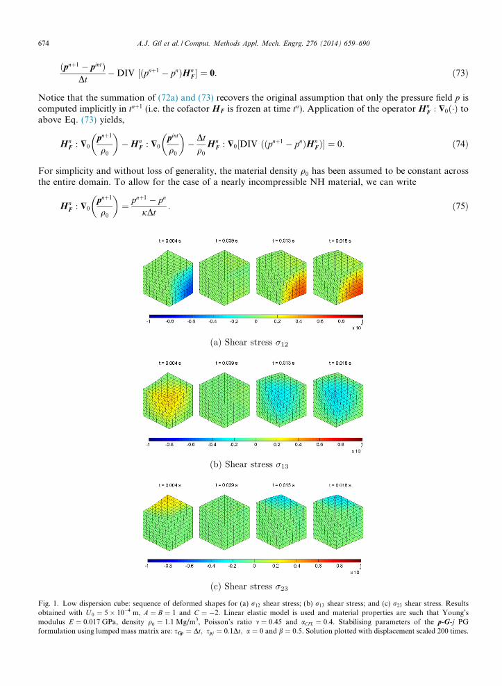
Fig. 1.obtainmodulformu
674 A.J. Gil et al. / Comput. Methods Appl. Mech. Engrg. 276 (2014) 659–690
ðpnþ1 � pintÞDt
�DIV ½ðpnþ1 � pnÞHnF � ¼ 0: ð73Þ
Notice that the summation of (72a) and (73) recovers the original assumption that only the pressure field p iscomputed implicitly in tnþ1 (i.e. the cofactor HF is frozen at time tn). Application of the operator Hn
F : $0ð�Þ toabove Eq. (73) yields,
HnF : $0
pnþ1
q0
� ��Hn
F : $0
pint
q0
� �� Dt
q0
HnF : $0½DIV ððpnþ1 � pnÞHn
FÞ� ¼ 0: ð74Þ
For simplicity and without loss of generality, the material density q0 has been assumed to be constant acrossthe entire domain. To allow for the case of a nearly incompressible NH material, we can write
HnF : $0
pnþ1
q0
� �¼ pnþ1 � pn
jDt: ð75Þ
Low dispersion cube: sequence of deformed shapes for (a) r12 shear stress; (b) r13 shear stress; and (c) r23 shear stress. Resultsed with U 0 ¼ 5� 10�4 m, A ¼ B ¼ 1 and C ¼ �2. Linear elastic model is used and material properties are such that Young’sus E ¼ 0:017 GPa, density q0 ¼ 1:1 Mg/m3, Poisson’s ratio m ¼ 0:45 and aCFL ¼ 0:4. Stabilising parameters of the p-G-j PGlation using lumped mass matrix are: sGp ¼ Dt; spj ¼ 0:1Dt; a ¼ 0 and b ¼ 0:5. Solution plotted with displacement scaled 200 times.
A.J. Gil et al. / Comput. Methods Appl. Mech. Engrg. 276 (2014) 659–690 675
For a truly incompressible material, j ¼ 1 and the right hand side of above equation vanishes resulting in theincompressibility constraint. Using this relationship on the first term of (74), it yields
Fig. 2.and stconverproperparam
pnþ1 � pn
jDt�Hn
F : $0
pint
q0
� �� Dt
q0
HnF : $0½DIV ððpnþ1 � pnÞHn
FÞ� ¼ 0: ð76Þ
3.4.1. Variational nonlinear fractional step formulation
To obtain a variational statement, we first define the residuals of Eqs. (72a), (72b), (73) and (76) as
Rpint :¼ DIV Pdev;n þDIV ðpnHnFÞ þ q0bn � ðp
int � pnÞDt
; ð77aÞ
RF :¼ $0pn
q0
� �� ðF
nþ1 � FnÞDt
; ð77bÞ
RJ :¼ HnF : $0
pint
q0
� �þ Dt
q0
HnF : $0½DIV ððpnþ1 � pnÞHn
FÞ� �ðpnþ1 � pnÞ
jDt; ð77cÞ
Rp :¼ DIV ðpnþ1 � pnÞHnF
�� ðp
nþ1 � pintÞDt
: ð77dÞ
Using appropriate stabilised conjugate virtual fields dVst ¼ ½dvst; dPst; dqst�T , already defined in (64), a varia-tional statement is defined by
dW PG ¼Z
Vdvst �Rvint dV þ
ZV
dPst : RF dV þZ
VdqstRJ dV ¼ 0: ð78Þ
Following a similar finite element spatial discretisation as that presented in the previous section, wherefp;F; pg and fdvst; dPst; dqstg are expanded in terms of linear shape functions, the resulting predictor systemof equations yields
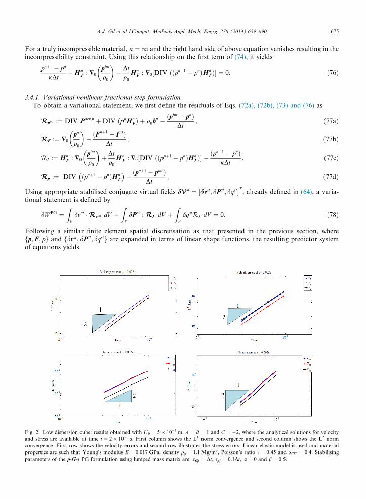
Low dispersion cube: results obtained with U 0 ¼ 5� 10�4 m, A ¼ B ¼ 1 and C ¼ �2, where the analytical solutions for velocityress are available at time t ¼ 2� 10�3 s. First column shows the L1 norm convergence and second column shows the L2 normgence. First row shows the velocity errors and second row illustrates the stress errors. Linear elastic model is used and materialties are such that Young’s modulus E ¼ 0:017 GPa, density q0 ¼ 1:1 Mg/m3, Poisson’s ratio m ¼ 0:45 and aCFL ¼ 0:4. Stabilisingeters of the p-G-j PG formulation using lumped mass matrix are: sGp ¼ Dt, spj ¼ 0:1Dt; a ¼ 0 and b ¼ 0:5.
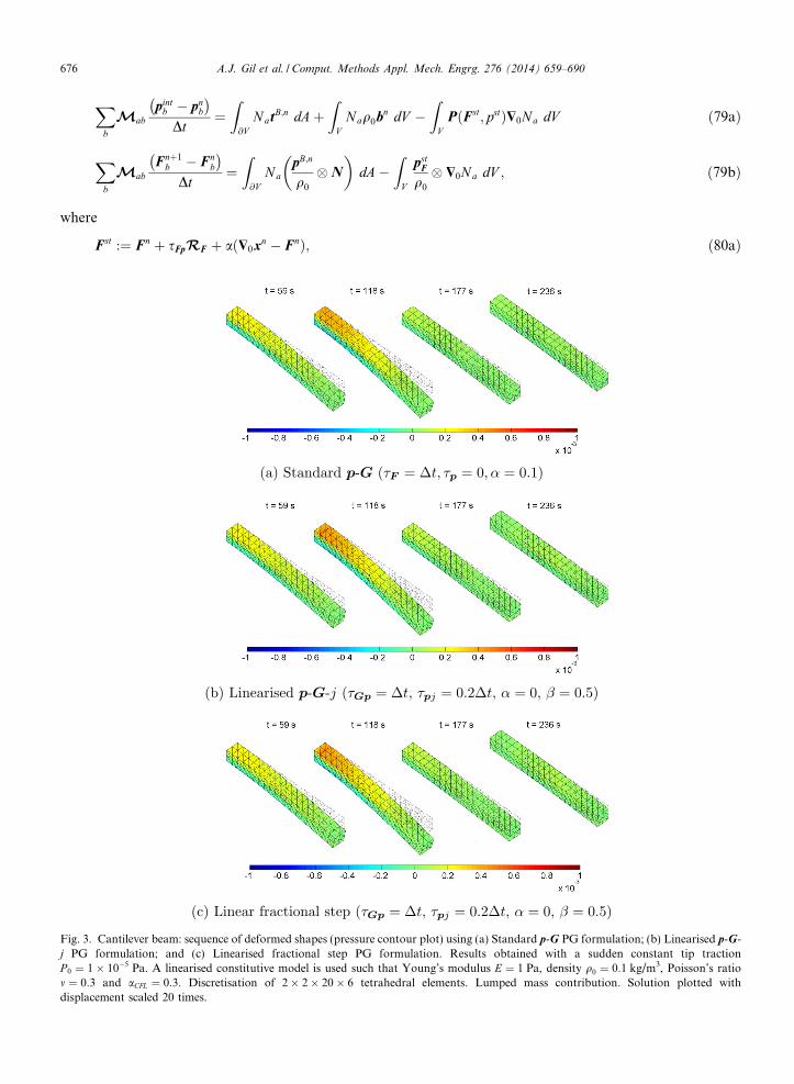
Fig. 3.j PGP 0 ¼ 1m ¼ 0:3displac
676 A.J. Gil et al. / Comput. Methods Appl. Mech. Engrg. 276 (2014) 659–690
Xb
Mabpint
b � pnb
�Dt
¼Z@V
N atB;n dAþZ
VNaq0bn dV �
ZV
PðFst; pstÞ$0Na dV ð79aÞ
Xb
MabFnþ1
b � Fnb
�Dt
¼Z@V
NapB;n
q0
�N
� �dA�
ZV
pstF
q0
� $0N a dV ; ð79bÞ
where
Fst :¼ Fn þ sFpRF þ að$0xn � FnÞ; ð80aÞ
Cantilever beam: sequence of deformed shapes (pressure contour plot) using (a) Standard p-G PG formulation; (b) Linearised p-G-formulation; and (c) Linearised fractional step PG formulation. Results obtained with a sudden constant tip traction� 10�5 Pa. A linearised constitutive model is used such that Young’s modulus E ¼ 1 Pa, density q0 ¼ 0:1 kg/m3, Poisson’s ratio
and aCFL ¼ 0:3. Discretisation of 2� 2� 20� 6 tetrahedral elements. Lumped mass contribution. Solution plotted withement scaled 20 times.
A.J. Gil et al. / Comput. Methods Appl. Mech. Engrg. 276 (2014) 659–690 677
pst :¼ pn þ sJplRJ þ bl det ð$0xnÞ � 1� pn
j
� �; ð80bÞ
pstF :¼ pn þ spFR
intp : ð80cÞ
Analogously to Section 2.4.1, by using linear shape functions for the expansion of ðpnþ1 � pnÞHnF in the second
term of the right hand side of Eq. (77c), this term vanishes when computed as part of the second term on theright hand side of (80b). For an incompressible medium where j ¼ 1 the term in parenthesis on the righthand side of (80b) reduces to the volumetric constraint. This Eq. (80b) is consistent with (71b), as multiplica-tion of (71b) by j yields (80b).
Setting spF = sJp ¼ 0, Eqs. (79a) and (79b) can be solved sequentially. The corrector step is formulated as
XbMvolab þ
Dt2
q0
Kab
� �pnþ1
b � pnb
Dt
� �¼Z@V
pB
q0
�HnFNN adA�
ZV
pstJ
q0
�HnF$0N a dV ; ð81Þ
where the mass matrix contribution Mvolab , the viscosity matrix contribution Kab and the stabilised linear
momentum pstJ are defined as
Mvolab :¼
ZV
1
jN aNb dV ; ð82aÞ
Kab :¼Z
VHn
F$0Na
�� Hn
F$0N b
�dV ; ð82bÞ
pstJ :¼ pint þ spJRpint ; ð82cÞ
respectively. In addition, in Eq. (81), terms HnF
�T pB
q0and Hn
F
�T pstJ
q0appearing in both integrands in the right
hand side are linearly approximated within every finite element. It is now possible to update the linear
momentum pnþ1 using the conventional Bubnov–Galerkin (BG) formulation dW BG ¼R
V dv �Rp dV to give
XbMabpnþ1
b � pintb
Dt¼Z
VNaDIV ðpnþ1 � pnÞHn
F
�dV : ð83Þ
The algorithm is finally evolved in time via a TVD-RK time integrator with a time step limit controlled by theshear wave speed cs
4. Numerical examples
In this section, a number of numerical examples will be presented in order to assess the performance of theenhanced p-F-J (p-G-j in small deformations) Petrov–Galerkin (PG) formulation in compressible, nearly
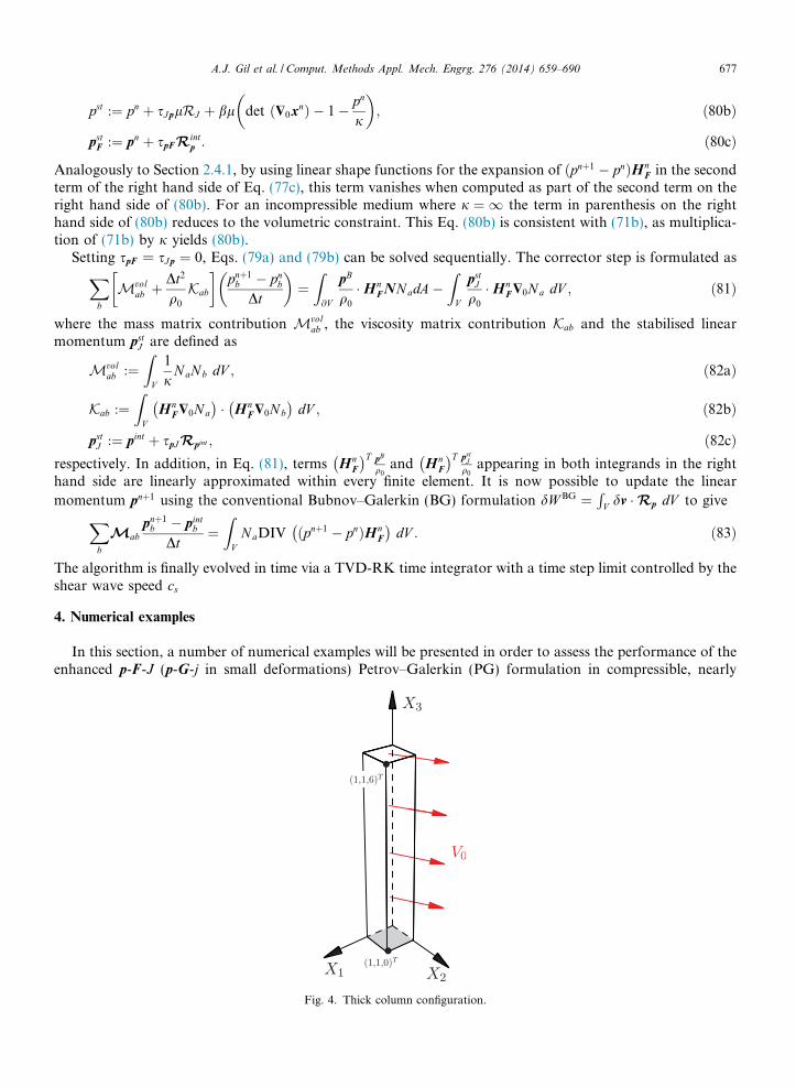
Fig. 4. Thick column configuration.
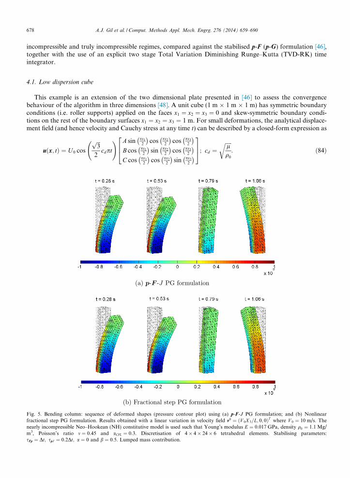
678 A.J. Gil et al. / Comput. Methods Appl. Mech. Engrg. 276 (2014) 659–690
incompressible and truly incompressible regimes, compared against the stabilised p-F (p-G) formulation [46],together with the use of an explicit two stage Total Variation Diminishing Runge–Kutta (TVD-RK) timeintegrator.
4.1. Low dispersion cube
This example is an extension of the two dimensional plate presented in [46] to assess the convergencebehaviour of the algorithm in three dimensions [48]. A unit cube (1 m � 1 m � 1 m) has symmetric boundaryconditions (i.e. roller supports) applied on the faces x1 ¼ x2 ¼ x3 ¼ 0 and skew-symmetric boundary condi-tions on the rest of the boundary surfaces x1 ¼ x2 ¼ x3 ¼ 1 m. For small deformations, the analytical displace-ment field (and hence velocity and Cauchy stress at any time t) can be described by a closed-form expression as
Fig. 5fractionearlym3, PsFp ¼ D
uðx; tÞ ¼ U 0 cos
ffiffiffi3p
2cdpt
! A sin px1
2
�cos px2
2
�cos px3
2
�B cos px1
2
�sin px2
2
�cos px3
2
�C cos px1
2
�cos px2
2
�sin px3
2
�264
375; cd ¼
ffiffiffiffiffilq0
r: ð84Þ
. Bending column: sequence of deformed shapes (pressure contour plot) using (a) p-F-J PG formulation; and (b) Nonlinearnal step PG formulation. Results obtained with a linear variation in velocity field v0 ¼ ðV 0X 3=L; 0; 0ÞT where V 0 ¼ 10 m/s. Theincompressible Neo–Hookean (NH) constitutive model is used such that Young’s modulus E ¼ 0:017 GPa, density q0 ¼ 1:1 Mg/oisson’s ratio m ¼ 0:45 and aCFL ¼ 0:3. Discretisation of 4� 4� 24� 6 tetrahedral elements. Stabilising parameters:t; spJ ¼ 0:2Dt; a ¼ 0 and b ¼ 0:5. Lumped mass contribution.
A.J. Gil et al. / Comput. Methods Appl. Mech. Engrg. 276 (2014) 659–690 679
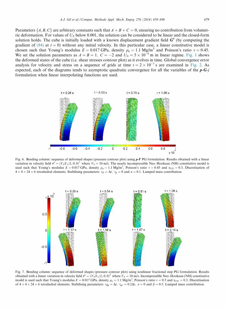
Parameters fA;B;Cg are arbitrary constants such that Aþ Bþ C ¼ 0, ensuring no contribution from volumet-ric deformation. For values of U 0 below 0.001, the solution can be considered to be linear and the closed-formsolution holds. The cube is initially loaded with a known displacement gradient field G0 (by computing thegradient of (84) at t ¼ 0) without any initial velocity. In this particular case, a linear constitutive model ischosen such that Young’s modulus E ¼ 0:017 GPa, density q0 ¼ 1:1 Mg/m3 and Poisson’s ratio m ¼ 0:45.We set the solution parameters as A ¼ B ¼ 1; C ¼ �2 and U 0 ¼ 5� 10�4 m in linear regime. Fig. 1 showsthe deformed states of the cube (i.e. shear stresses contour plot) as it evolves in time. Global convergence erroranalysis for velocity and stress on a sequence of grids at time t ¼ 2� 10�3 s are examined in Fig. 2. Asexpected, each of the diagrams tends to asymptotic quadratic convergence for all the variables of the p-G-jformulation when linear interpolating functions are used.
Fig. 6. Bending column: sequence of deformed shapes (pressure contour plot) using p-F PG formulation. Results obtained with a linearvariation in velocity field v0 ¼ ðV 0X 3=L; 0; 0ÞT where V 0 ¼ 10 m/s. The nearly incompressible Neo–Hookean (NH) constitutive model isused such that Young’s modulus E ¼ 0:017 GPa, density q0 ¼ 1:1 Mg/m3, Poisson’s ratio m ¼ 0:45 and aCFL ¼ 0:3. Discretisation of4� 4� 24� 6 tetrahedral elements. Stabilising parameters: sF ¼ Dt; sp ¼ 0 and a ¼ 0:1. Lumped mass contribution.
Fig. 7. Bending column: sequence of deformed shapes (pressure contour plot) using nonlinear fractional step PG formulation. Resultsobtained with a linear variation in velocity field v0 ¼ ðV 0X 3=L; 0; 0ÞT where V 0 ¼ 10 m/s. Incompressible Neo–Hookean (NH) constitutivemodel is used such that Young’s modulus E ¼ 0:017 GPa, density q0 ¼ 1:1 Mg/m3, Poisson’s ratio m ¼ 0:5 and aCFL ¼ 0:3. Discretisationof 4� 4� 24� 6 tetrahedral elements. Stabilising parameters: sFp ¼ Dt; spJ ¼ 0:2Dt; a ¼ 0 and b ¼ 0:5. Lumped mass contribution.
680 A.J. Gil et al. / Comput. Methods Appl. Mech. Engrg. 276 (2014) 659–690
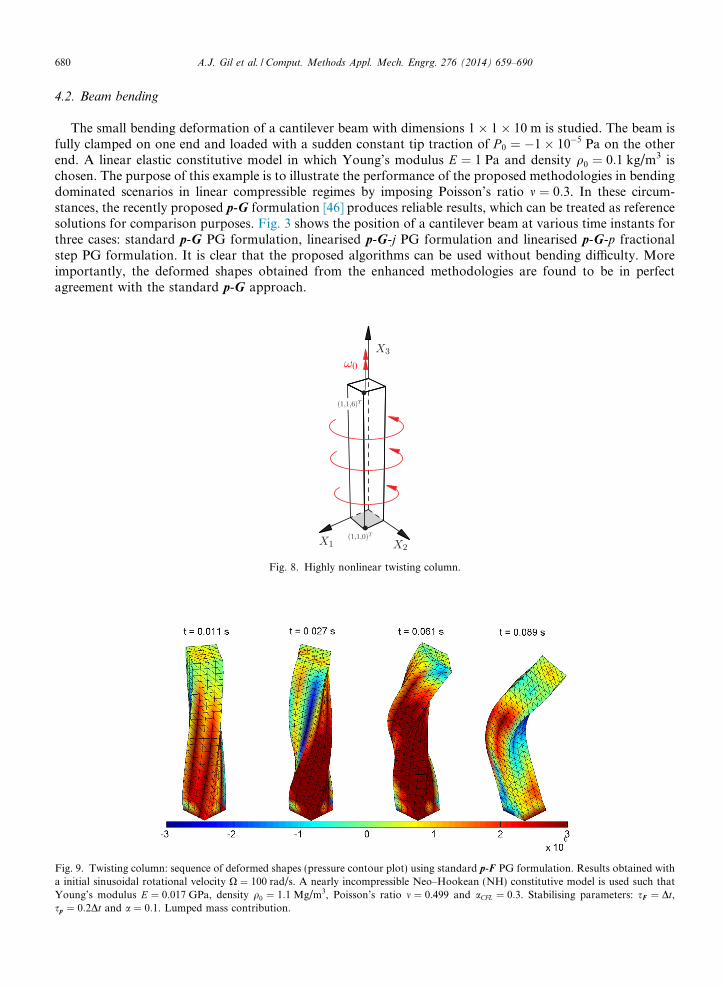
4.2. Beam bending
The small bending deformation of a cantilever beam with dimensions 1� 1� 10 m is studied. The beam isfully clamped on one end and loaded with a sudden constant tip traction of P 0 ¼ �1� 10�5 Pa on the otherend. A linear elastic constitutive model in which Young’s modulus E ¼ 1 Pa and density q0 ¼ 0:1 kg/m3 ischosen. The purpose of this example is to illustrate the performance of the proposed methodologies in bendingdominated scenarios in linear compressible regimes by imposing Poisson’s ratio m ¼ 0:3. In these circum-stances, the recently proposed p-G formulation [46] produces reliable results, which can be treated as referencesolutions for comparison purposes. Fig. 3 shows the position of a cantilever beam at various time instants forthree cases: standard p-G PG formulation, linearised p-G-j PG formulation and linearised p-G-p fractionalstep PG formulation. It is clear that the proposed algorithms can be used without bending difficulty. Moreimportantly, the deformed shapes obtained from the enhanced methodologies are found to be in perfectagreement with the standard p-G approach.
Fig. 8. Highly nonlinear twisting column.
Fig. 9. Twisting column: sequence of deformed shapes (pressure contour plot) using standard p-F PG formulation. Results obtained witha initial sinusoidal rotational velocity X ¼ 100 rad/s. A nearly incompressible Neo–Hookean (NH) constitutive model is used such thatYoung’s modulus E ¼ 0:017 GPa, density q0 ¼ 1:1 Mg/m3, Poisson’s ratio m ¼ 0:499 and aCFL ¼ 0:3. Stabilising parameters: sF ¼ Dt,sp ¼ 0:2Dt and a ¼ 0:1. Lumped mass contribution.
A.J. Gil et al. / Comput. Methods Appl. Mech. Engrg. 276 (2014) 659–690 681
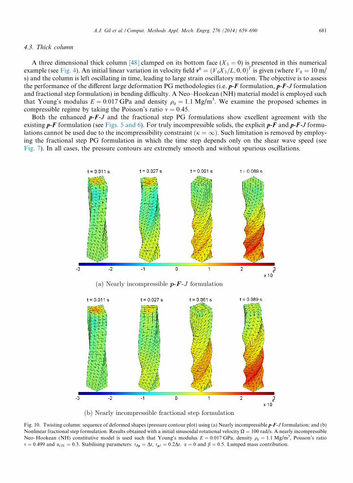
4.3. Thick column
A three dimensional thick column [48] clamped on its bottom face (X 3 ¼ 0) is presented in this numericalexample (see Fig. 4). An initial linear variation in velocity field v0 ¼ ðV 0X 3=L; 0; 0ÞT is given (where V 0 ¼ 10 m/s) and the column is left oscillating in time, leading to large strain oscillatory motion. The objective is to assessthe performance of the different large deformation PG methodologies (i.e. p-F formulation, p-F-J formulationand fractional step formulation) in bending difficulty. A Neo–Hookean (NH) material model is employed suchthat Young’s modulus E ¼ 0:017 GPa and density q0 ¼ 1:1 Mg/m3. We examine the proposed schemes incompressible regime by taking the Poisson’s ratio m ¼ 0:45.
Both the enhanced p-F-J and the fractional step PG formulations show excellent agreement with theexisting p-F formulation (see Figs. 5 and 6). For truly incompressible solids, the explicit p-F and p-F-J formu-lations cannot be used due to the incompressibility constraint ðj ¼ 1Þ. Such limitation is removed by employ-ing the fractional step PG formulation in which the time step depends only on the shear wave speed (seeFig. 7). In all cases, the pressure contours are extremely smooth and without spurious oscillations.
Fig. 10. Twisting column: sequence of deformed shapes (pressure contour plot) using (a) Nearly incompressible p-F-J formulation; and (b)Nonlinear fractional step formulation. Results obtained with a initial sinusoidal rotational velocity X ¼ 100 rad/s. A nearly incompressibleNeo–Hookean (NH) constitutive model is used such that Young’s modulus E ¼ 0:017 GPa, density q0 ¼ 1:1 Mg/m3, Poisson’s ratiom ¼ 0:499 and aCFL ¼ 0:3. Stabilising parameters: sFp ¼ Dt, spJ ¼ 0:2Dt; a ¼ 0 and b ¼ 0:5. Lumped mass contribution.
682 A.J. Gil et al. / Comput. Methods Appl. Mech. Engrg. 276 (2014) 659–690
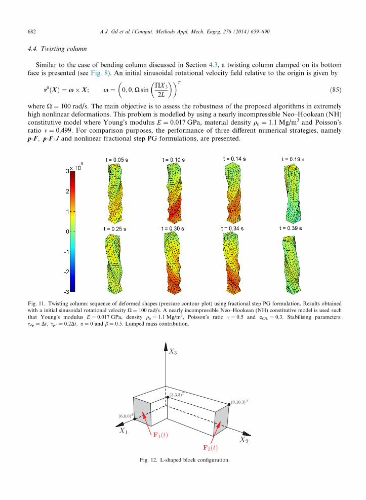
4.4. Twisting column
Similar to the case of bending column discussed in Section 4.3, a twisting column clamped on its bottomface is presented (see Fig. 8). An initial sinusoidal rotational velocity field relative to the origin is given by
Fig. 11with athat YsFp ¼ D
v0ðXÞ ¼ x� X ; x ¼ 0; 0;X sinPX 3
2L
� �� �T
ð85Þ
where X ¼ 100 rad/s. The main objective is to assess the robustness of the proposed algorithms in extremelyhigh nonlinear deformations. This problem is modelled by using a nearly incompressible Neo–Hookean (NH)constitutive model where Young’s modulus E ¼ 0:017 GPa, material density q0 ¼ 1:1 Mg/m3 and Poisson’sratio m ¼ 0:499. For comparison purposes, the performance of three different numerical strategies, namelyp-F; p-F-J and nonlinear fractional step PG formulations, are presented.
. Twisting column: sequence of deformed shapes (pressure contour plot) using fractional step PG formulation. Results obtainedinitial sinusoidal rotational velocity X ¼ 100 rad/s. A nearly incompressible Neo–Hookean (NH) constitutive model is used suchoung’s modulus E ¼ 0:017 GPa, density q0 ¼ 1:1 Mg/m3, Poisson’s ratio m ¼ 0:5 and aCFL ¼ 0:3. Stabilising parameters:t; spJ ¼ 0:2Dt; a ¼ 0 and b ¼ 0:5. Lumped mass contribution.
Fig. 12. L-shaped block configuration.
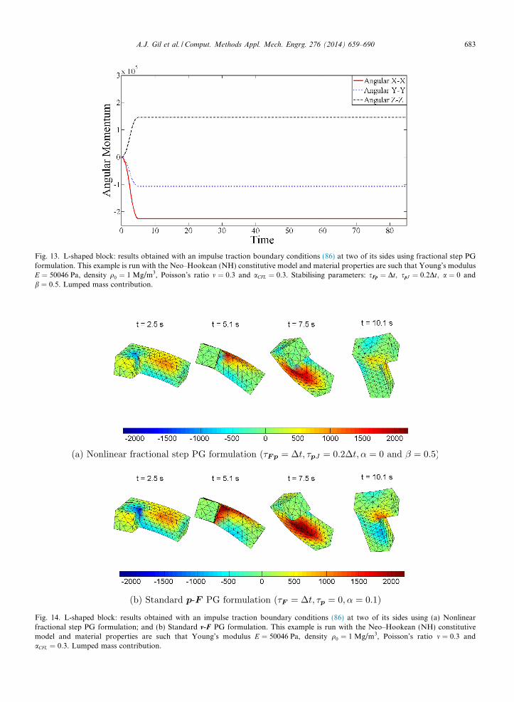
Fig. 13. L-shaped block: results obtained with an impulse traction boundary conditions (86) at two of its sides using fractional step PGformulation. This example is run with the Neo–Hookean (NH) constitutive model and material properties are such that Young’s modulusE ¼ 50046 Pa, density q0 ¼ 1 Mg/m3, Poisson’s ratio m ¼ 0:3 and aCFL ¼ 0:3. Stabilising parameters: sFp ¼ Dt; spJ ¼ 0:2Dt; a ¼ 0 andb ¼ 0:5. Lumped mass contribution.
Fig. 14. L-shaped block: results obtained with an impulse traction boundary conditions (86) at two of its sides using (a) Nonlinearfractional step PG formulation; and (b) Standard v-F PG formulation. This example is run with the Neo–Hookean (NH) constitutivemodel and material properties are such that Young’s modulus E ¼ 50046 Pa, density q0 ¼ 1 Mg/m3, Poisson’s ratio m ¼ 0:3 andaCFL ¼ 0:3. Lumped mass contribution.
A.J. Gil et al. / Comput. Methods Appl. Mech. Engrg. 276 (2014) 659–690 683
684 A.J. Gil et al. / Comput. Methods Appl. Mech. Engrg. 276 (2014) 659–690
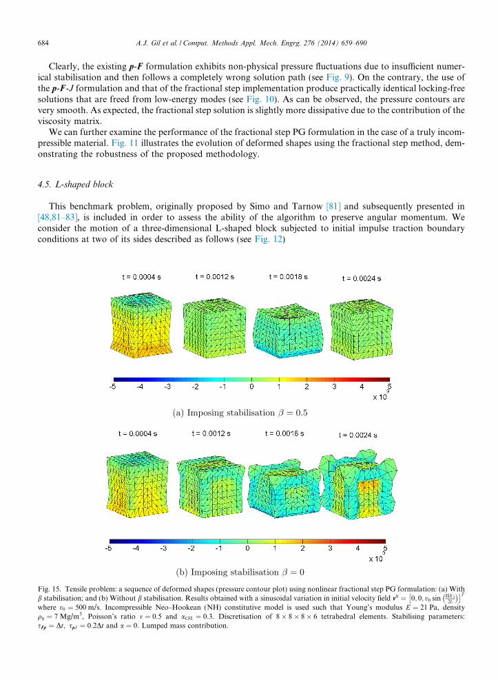
Clearly, the existing p-F formulation exhibits non-physical pressure fluctuations due to insufficient numer-ical stabilisation and then follows a completely wrong solution path (see Fig. 9). On the contrary, the use ofthe p-F-J formulation and that of the fractional step implementation produce practically identical locking-freesolutions that are freed from low-energy modes (see Fig. 10). As can be observed, the pressure contours arevery smooth. As expected, the fractional step solution is slightly more dissipative due to the contribution of theviscosity matrix.
We can further examine the performance of the fractional step PG formulation in the case of a truly incom-pressible material. Fig. 11 illustrates the evolution of deformed shapes using the fractional step method, dem-onstrating the robustness of the proposed methodology.
4.5. L-shaped block
This benchmark problem, originally proposed by Simo and Tarnow [81] and subsequently presented in[48,81–83], is included in order to assess the ability of the algorithm to preserve angular momentum. Weconsider the motion of a three-dimensional L-shaped block subjected to initial impulse traction boundaryconditions at two of its sides described as follows (see Fig. 12)
Fig. 15b stabiwhereq0 ¼ 7sFp ¼ D
. Tensile problem: a sequence of deformed shapes (pressure contour plot) using nonlinear fractional step PG formulation: (a) Withlisation; and (b) Without b stabilisation. Results obtained with a sinusoidal variation in initial velocity field v0 ¼ 0; 0; v0 sin PX 3
2L
�� T
v0 ¼ 500 m/s. Incompressible Neo–Hookean (NH) constitutive model is used such that Young’s modulus E ¼ 21 Pa, densityMg/m3, Poisson’s ratio m ¼ 0:5 and aCFL ¼ 0:3. Discretisation of 8� 8� 8� 6 tetrahedral elements. Stabilising parameters:t; spJ ¼ 0:2Dt and a ¼ 0. Lumped mass contribution.
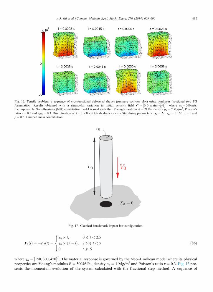
Fig. 16. Tensile problem: a sequence of cross-sectional deformed shapes (pressure contour plot) using nonlinear fractional step PGformulation. Results obtained with a sinusoidal variation in initial velocity field v0 ¼ 0; 0; v0 sin PX 3
2L
�� Twhere v0 ¼ 500 m/s.
Incompressible Neo–Hookean (NH) constitutive model is used such that Young’s modulus E ¼ 21 Pa, density q0 ¼ 7 Mg/m3, Poisson’sratio m ¼ 0:5 and aCFL ¼ 0:3. Discretisation of 8� 8� 8� 6 tetrahedral elements. Stabilising parameters: sFp ¼ Dt; spJ ¼ 0:1Dt; a ¼ 0 andb ¼ 0:5. Lumped mass contribution.
Fig. 17. Classical benchmark impact bar configuration.
A.J. Gil et al. / Comput. Methods Appl. Mech. Engrg. 276 (2014) 659–690 685
F1ðtÞ ¼ �F2ðtÞ ¼g0 � t; 0 6 t < 2:5
g0 � ð5� tÞ; 2:5 6 t < 5
0; t P 5
8><>: ð86Þ
where g0 ¼ ½150; 300; 450�T . The material response is governed by the Neo–Hookean model where its physicalproperties are Young’s modulus E ¼ 50046 Pa, density q0 ¼ 1 Mg/m3 and Poisson’s ratio m ¼ 0:3. Fig. 13 pre-sents the momentum evolution of the system calculated with the fractional step method. A sequence of
686 A.J. Gil et al. / Comput. Methods Appl. Mech. Engrg. 276 (2014) 659–690
deformed states is illustrated in Fig. 14(a), each of which agrees very well with the results obtained using p-Fformulation proposed in [46] (see Fig. 14(b)).
4.6. Tensile cube
The objective of this three dimensional tensile cube problem is to demonstrate the performance of the non-linear fractional step PG formulation when a tetrahedral mesh is used in an incompressible regime. A unitblock clamped at the bottom (traction-free conditions for the rest of the boundaries) is subjected to a sinusoi-
dal variation in initial velocity field v0 ¼ 0; 0; v0 sin PX 3
2L
�� T(where v0 ¼ 500 m/s) which is compatible with the
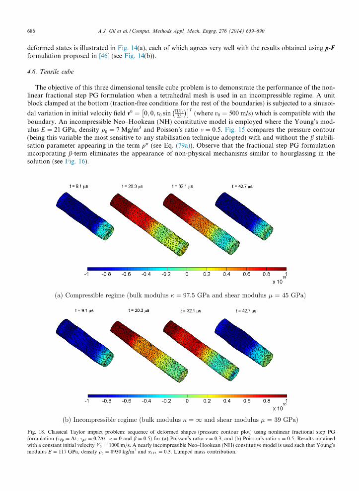
boundary. An incompressible Neo–Hookean (NH) constitutive model is employed where the Young’s mod-ulus E ¼ 21 GPa, density q0 ¼ 7 Mg/m3 and Poisson’s ratio m ¼ 0:5. Fig. 15 compares the pressure contour(being this variable the most sensitive to any stabilisation technique adopted) with and without the b stabili-sation parameter appearing in the term pst (see Eq. (79a)). Observe that the fractional step PG formulationincorporating b-term eliminates the appearance of non-physical mechanisms similar to hourglassing in thesolution (see Fig. 16).
Fig. 18. Classical Taylor impact problem: sequence of deformed shapes (pressure contour plot) using nonlinear fractional step PGformulation (sFp ¼ Dt; spJ ¼ 0:2Dt; a ¼ 0 and b ¼ 0:5) for (a) Poisson’s ratio m ¼ 0:3; and (b) Poisson’s ratio m ¼ 0:5. Results obtainedwith a constant initial velocity V 0 ¼ 1000 m=s. A nearly incompressible Neo–Hookean (NH) constitutive model is used such that Young’smodulus E ¼ 117 GPa, density q0 ¼ 8930 kg/m3 and aCFL ¼ 0:3. Lumped mass contribution.
A.J. Gil et al. / Comput. Methods Appl. Mech. Engrg. 276 (2014) 659–690 687
4.7. Benchmarked Taylor Impact problem
The classical benchmarking example demonstrates the impact of a cylindrical copper bar of initial radiusr0 ¼ 0:0032 m and length L0 ¼ 0:0324 m, against a rigid wall (see Fig. 17). The bar is made of a nearly incom-pressible Neo–Hookean (NH) constitutive model such that Young’s modulus E ¼ 117 GPa and densityq0 ¼ 8930 kg/m3 and is dropped with a constant velocity V 0 ¼ 1000 m/s. The primary interest of this problemis to show the effectiveness of the fractional step method in both compressible and truly incompressibleregimes, where in the latter case no volumetric deformation is allowed. Locking-free deformed sequencesbased on two different Poisson’s ratios are presented in Fig. 18. Observe that the pressure resolution is clearlyfreed from non-physical pressure checkerboard modes.
5. Conclusions
In this paper, a new computational methodology has been presented for the analysis of bending dominatednearly and truly incompressible large deformations in fast solid dynamics. The methodology is based upon asystem of first order conservation laws, where the linear momentum p conservation equation is supplementedwith two geometric conservation laws, one for the deformation gradient F and one for the Jacobian of thedeformation J. A Petrov–Galerkin spatial discretisation method has been employed for stabilisation of thegoverning equations and an adapted fractional step method has been presented when dealing with nonlineardeformations in the incompressible limit. Both velocities (or displacements) and stresses display the same rateof convergence, which proves ideal in the case of low order finite elements (usually preferred in commercialcodes). It has been shown that the enhanced p-F-J formulation overcomes locking and non-physical hydro-static fluctuations in the pressure, providing a good balance between accuracy and speed of computation.The consideration of polyconvex energy functionals [84,85] to enable the definition of generalised convexentropies is the next step of our work. This will allow the transformation of the system of conservation lawsinto a symmetric set of quasilinear hyperbolic equations.
Acknowledgements
The first author acknowledges the financial support received through “The Leverhulme Prize” awarded byThe Leverhulme Trust, United Kingdom. The third author would like to acknowledge the financial supportprovided by the Ser Cymru National Research Network for Advanced Engineering and Materials.
References
[1] J.O. Hallquist, LS-DYNA theoretical manual, Livermore Software Technology Corporation, 1998.[2] J.O. Hallquist, LS-DYNA keyword user’s manual, Livermore Software Technology Corporation, 2003.[3] D.J. Benson, Computational methods in Lagrangian and Eulerian hydrocodes, Comput. Methods Appl. Mech. Eng. 99 (1992) 235–
394.[4] D.P. Flanagan, T. Belytschko, A uniform strain hexahedron and quadrilateral with orthogonal hourglass control, Int. J. Numer.
Methods Eng. 17 (1981) 679–706.[5] G.L. Goudreau, J.O. Hallquist, Recent developments in large scale Lagrangian hydrocodes, Comput. Methods Appl. Mech. Eng. 33
(1982) 725–757.[6] Hibbitt, Karlsson, Sorensen, ABAQUS/Explicit: User’s manual (volume 1, version 6.1), 2000.[7] PAM-CRASH/PAM-SAFE: Solver reference with manual, PAM SYSTEM International, 2002.[8] D.J. Payen, K.J. Bathe, A stress improvement procedure, Comput. Struct. 112-113 (2012) 311–326.[9] D.J. Payen, K.J. Bathe, Improved stresses for the 4-node tetrahedral element, Comput. Struct. 89 (2011) 1265–1273.
[10] C.H. Lee, A.J. Gil, J. Bonet, Development of a cell centred upwind finite volume algorithm for a new conservation law formulation instructural dynamics, Comput. Struct. 118 (2013) 13–38.
[11] C.R. Dohrmann, M.W. Heinstein, J. Jung, S.W. Key, W.R. Witkowski, Node-based uniform strain elements for three-nodetriangular and four-node tetrahedral meshes, Int. J. Numer. Methods Eng. 47 (2000) 1549–1568.
[12] T. Belytschko, W.K. Liu, B. Moran, Nonlinear Finite Elements for Continua and Structures, John Wiley and Sons, 2000.[13] K.J. Bathe, Finite Element Procedures, Prentice Hall, 1996.[14] N.M. Newmark, A method of computation for structural dynamics, J. Eng. Mech. Div. 85 (1959) 67–94.[15] T.J.R. Hughes, The Finite Element Method: Linear Static and Dynamic Finite Element Analysis, Dover Publications, 2000.
688 A.J. Gil et al. / Comput. Methods Appl. Mech. Engrg. 276 (2014) 659–690
[16] H.M. Hilber, T.J.R. Hughes, R.L. Taylor, Improved numerical dissipation for time integration algorithms in structural dynamics,Earthquake Eng. Struct. Dyn. 5 (1977) 283–292.
[17] W.L. Wood, M. Bossak, O.C. Zienkiewicz, An alpha modification of Newmark’s method, Int. J. Numer. Methods Eng. 15 (1980)1562–1566.
[18] J. Chung, G.M. Hulbert, A time integration algorithm for structural dynamics with improved numerical dissipation: the generalized amethod, J. Appl. Mech. 60 (1993) 371–375.
[19] D.D. Adams, W.L. Wood, Comparison of Hilber–Hughes–Taylor and Bossak a method for the numerical integration of vibrationequations, Int. J. Numer. Methods Eng. 19 (1983) 765–771.
[20] K. Washizu, Variational Methods in Elasticity and Plasticity, Pergamon Press, Oxford, 1975.[21] J.C. Nagtegaal, D.M. Park, J.R. Rice, On numerically accurate finite element solutions in the fully plastic range, Comput. Methods
Appl. Mech. Eng. 4 (1974) 153–177.[22] J.H. Argyris, P.C. Dunne, T. Angelopoulos, B. Bichat, Large natural strains and some special difficulties due to nonlinearity and
incompressibility in finite elements, Comput. Methods Appl. Mech. Eng. 4 (1974) 219–278.[23] D.S. Malkus, T.J.R. Hughes, Mixed finite element methods – reduced and selective integration techniques: a unification of concepts,
Comput. Methods Appl. Mech. Eng. 15 (1978) 63–81.[24] T.J.R. Hughes, Generalization of selective integration procedures to anisotropic and nonlinear media, Int. J. Numer. Methods Eng.
15 (1980) 1413–1418.[25] J.C. Simo, R.L. Taylor, K.S. Pister, Variational and projection methods for the volume constraint in finite deformation elasto-
plasticity, Comput. Methods Appl. Mech. Eng. 51 (1985) 177–208.[26] E.A. de Souza Neto, D. Peric, M. Dutko, D.R.J. Owen, Design of simple low order finite elements for large strain analysis of nearly
incompressible solids, Int. J. Solids Struct. 33 (1996) 3277–3296.[27] T. Sussman, K.J. Bathe, A finite element formulation for nonlinear incompressible elastic and inelastic analysis, Comput. Struct. 26
(1987) 357–409.[28] B. Moran, M. Ortiz, C.F. Shih, Formulation of implicit finite element methods for multiplicative finite deformation plasticity, Int. J.
Numer. Methods Eng. 29 (1990) 483–514.[29] J.C. Simo, F. Armero, Geometrically non-linear enhanced strain mixed methods and the method of incompatible modes, Int. J.
Numer. Methods Eng. 33 (1992) 1413–1449.[30] A.J. Gil, P.D. Ledger, A coupled hp-finite element scheme for the solution of two-dimensional electrostrictive materials, Int. J.
Numer. Methods Eng. 91 (2012) 1158–1183.[31] D. Jin, P.D. Ledger, A.J. Gil, An hp-fem framework for the simulation of electrostrictive and magnetostrictive materials, Comput.
Struct. 133 (2014) 131–148.[32] J. Bonet, A.J. Burton, A simple average nodal pressure tetrahedral element for incompressible and nearly incompressible dynamic
explicit applications, Commun. Numer. Methods Eng. 14 (1998) 437–449.[33] J. Bonet, H. Marriott, O. Hassan, An averaged nodal deformation gradient linear tetrahedral element for large strain explicit dynamic
applications, Commun. Numer. Methods Eng. 17 (2001) 551–561.[34] M.W. Gee, C.R. Dohrmann, S.W. Key, W.A. Wall, A uniform nodal strain tetrahedron with isochoric stabilization, Int. J. Numer.
Methods Eng. 78 (2009) 429–443.[35] M.A. Puso, J. Solberg, A stabilized nodally integrated tetrahedral, Int. J. Numer. Methods Eng. 67 (2006) 841–867.[36] O.C. Zienkiewicz, J. Rojek, R.L. Taylor, M. Pastor, Triangles and tetrahedra in explicit dynamic codes for solids, Int. J. Numer.
Methods Eng. 43 (1998) 565–583.[37] J. Bonet, H. Marriott, O. Hassan, Stability and comparison of different linear tetrahedral formulations for nearly incompressible
explicit dynamic applications, Int. J. Numer. Methods Eng. 50 (2001) 119–133.[38] F.M.A. Pires, E.A. de Souza Neto, J.L. de la Cuesta Padilla, An assessment of the average nodal volume formulation for the analysis
of nearly incompressible solids under finite strains, Commun. Numer. Methods Eng. 20 (2004) 569–583.[39] T.J.R. Hughes, L.P. Franca, M. Balestra, A new finite element formulation for computational fluid dynamics: V. Circumventing the
Babuska–Brezzi condition: a stable Petrov–Galerkin formulation of the Stokes problem accommodating equal-order interpolations,Comput. Methods Appl. Mech. Eng. 59 (1986) 85–99.
[40] F. Brezzi, On the existence, uniqueness and approximation of saddle-point problems arising from lagrangian multipliers, ESAIM:Math. Model. Numer. Anal. – Modelisation Mathematique et Analyse Numerique 8 (1974) 129–151.
[41] B.A. Szabo, I. Babuska, Finite Element Analysis, John Wiley and Sons, 1991.[42] W. Elmer, J.S. Chen, M. Puso, E. Taciroglu, A stable, meshfree, nodal integration method for nearly incompressible solids, Finite
Elem. Anal. Des. 51 (2012) 81–85.[43] M. Cervera, M. Chiumenti, R. Codina, Mixed stabilized finite element methods in nonlinear solid mechanics. Part I: Formulation,
Comput. Methods Appl. Mech. Eng. 199 (2010) 2559–2570.[44] F. Auricchio, L.B. da Veiga, C. Lovadina, A. Reali, R.L. Taylor, P. Wriggers, Approximation of incompressible large deformation
elastic problems: some unresolved issues, Comput. Mech. (2013) 1–15.[45] J. Schroder, P. Wriggers, D. Balzani, A new mixed finite element based on different approximations of the minors of deformation
tensors, Comput. Methods Appl. Mech. Eng. 200 (2011) 3583–3600.[46] C.H. Lee, A.J. Gil, J. Bonet, Development of a stabilised Petrov–Galerkin formulation for conservation laws in Lagrangian fast solid
dynamics, Comput. Methods Appl. Mech. Eng. 268 (2014) 40–64.[47] I. A. Karim, C. H. Lee, A. J. Gil, J. Bonet, A two-step Taylor Galerkin formulation for fast dynamics, Eng. Comput. 31, in press.
http://dx.doi.org/10.1108/EC-12-2012-0319.
A.J. Gil et al. / Comput. Methods Appl. Mech. Engrg. 276 (2014) 659–690 689
[48] M. Aguirre, A.J. Gil, J. Bonet, A.A. Carreno, A vertex centred finite volume Jameson–Schmidt–Turkel (JST) algorithm for a mixedconservation formulation in solid dynamics, J. Comput. Phys. 259 (2014) 672–699.
[49] G. Scovazzi, Lagrangian shock hydrodynamics on tetrahedral meshes: a stable and accurate variational multiscale approach, J.Comput. Phys. 231 (2012) 8029–8069.
[50] G. Scovazzi, M.A. Christon, T.J.R. Hughes, J.N. Shadid, Stabilized shock hydrodynamics: I. A Lagrangian method, Comput.Methods Appl. Mech. Eng. 196 (2007) 923–966.
[51] G. Scovazzi, Stabilized shock hydrodynamics: II. Design and physical interpretation of the SUPG operator for Lagrangiancomputations, Comput. Methods Appl. Mech. Eng. 196 (2007) 967–978.
[52] G. Scovazzi, J.N. Shadid, E. Love, W.J. Rider, A conservative nodal variational multiscale method for Lagrangian shockhydrodynamics, Comput. Methods Appl. Mech. Eng. 199 (2010) 3059–3100.
[53] A.J. Gil, J. Bonet, J. Silla, O. Hassan, A discrete geometric conservation law (DGCL) for a cell vertex finite-volume algorithm onmoving domains, Int. J. Numer. Methods Biomed. Eng. 26 (2010) 770–779.
[54] R. Courant, K. Friedrichs, H. Lewy, On the partial difference equations of mathematical physics, Mathematische Annalem 100 (1928)32–74.
[55] A.J. Chorin, The numerical solution of the Navier–Stokes equations for an incompressible fluid, Bull. Am. Math. Soc. 73 (1967) 928–931.
[56] A.J. Chorin, Numerical solution of the Navier–Stokes equations, Math. Comput. 22 (1968) 745–762.[57] A.J. Chorin, On the convergence of discrete approximations to the Navier–Stokes equations, Math. Comput. 23 (1969) 341–353.[58] A.J. Gil, A.A. Carreno, J. Bonet, O. Hassan, The immersed structural potential method for haemodynamic applications, J. Comput.
Phys. 229 (2011) 8613–8641.[59] A.J. Gil, A.A. Carreno, J. Bonet, O. Hassan, An enhanced immersed structural potential method for fluid-structure interaction, J.
Comput. Phys. 250 (2013) 178–205.[60] S.K. Lahiri, J. Bonet, J. Peraire, L. Casals, A variationally consistent fractional time-step integration method for incompressible and
nearly incompressible Lagrangian dynamics, Int. J. Numer. Methods Eng. 63 (2005) 1371–1395.[61] J.E. Marsden, T.J.R. Hughes, Mathematical Foundations of Elasticity, Dover Publications, 1994.[62] T.J.R. Hughes, L.P. Franca, M. Mallet, A new finite element formulation for computational fluid dynamics: I. Symmetric forms of
the compressible Euler and Navier–Stokes equations and the second law of thermodynamics, Comput. Methods Appl. Mech. Eng. 54(1986) 223–234.
[63] Q. Tiehu, Symmetrizing nonlinear elastodynamic system, J. Elast. 50 (1998) 245–252.[64] J. Bonet, R.D. Wood, Nonlinear Continuum Mechanics for Finite Element Analysis, second ed., Cambridge University Press, 2008.[65] T.J.R. Hughes, G. Scovazzi, T.E. Tezduyar, Stabilized methods for compressible flows, J. Sci. Comput. 43 (2010) 343–368.[66] T.J.R. Hughes, T.E. Tezduyar, Finite element methods for first-order hyperbolic systems with particular emphasis on the
compressible Euler equations, Comput. Methods Appl. Mech. Eng. 45 (1984) 217–284.[67] T.J.R. Hughes, L.P. Franca, M. Mallet, A new finite element formulation for computational fluid dynamics: Vi. Convergence analysis
of the generalized SUPG formulation for linear time-dependent multidimensional advective-diffusive systems, Comput. MethodsAppl. Mech. Eng. 63 (1987) 97–112.
[68] T.E. Tezduyar, T.J.R. Hughes, Development of time-accurate finite element techniques for first-order hyperbolic systems withparticular emphasis on the compressible Euler equations, NASA Technical Report NASA-CR-204772, NASA, 1982.
[69] T.E. Tezduyar, T.J.R. Hughes, Finite element formulations for convection dominated flows with particular emphasis on thecompressible Euler equations, in: Proceedings of AIAA 21st Aaerospace Sciences Meeting, AIAA paper 83-0125, Reno, Nevada,1983.
[70] T.J.R. Hughes, Multiscale phenomena: Green’s functions, the Dirichlet-to-Neumann formulation, subgrid scale models, bubbles andthe origins of stabilized methods, Comput. Methods Appl. Mech. Eng. 127 (1995) 387–401.
[71] T.J.R. Hughes, G.R. Feijoo, L. Mazzei, J.-B. Quincy, The variational multiscale method – a paradigm for computational mechanics,Comput. Methods Appl. Mech. Eng. 166 (1998) 3–24.
[72] T.J.R. Hughes, G. Scovazzi, L.P. Franca, in: E. Stein, R. de Borst, T.J.R. Hughes (Eds.), Encyclopedia of Computational Mechanics,John Wiley and Sons, 2004.
[73] G. Scovazzi, E. Love, M.J. Shashkov, A multi-scale Q1/P0 approach to Lagrangian shock hydrodynamics, Comput. Methods Appl.Mech. Eng. 197 (2008) 1056–1079.
[74] C.W. Shu, Efficient implementation of essentially non-oscillatory shock capturing schemes, J. Comput. Phys. 77 (1988) 439–471.[75] R. Codina, Pressure stability in fractional step finite element methods for incompressible flows, J. Comput. Phys. 170 (2001) 112–140.[76] J. Donea, A. Huerta, Finite Element Methods for Flow Problems, Wiley and Sons, 2004.[77] A.J. Gil, Z. Zhang, O. Hassan, K. Morgan, Parallel multigrid detached eddy simulation algorithm for three-dimensional unsteady
incompressible flows on unstructured grids, J. Aerosp. Eng. 19 (2006) 271–280.[78] O. Gonzalez, A.M. Stuart, A First Course in Continuum Mechanics, Cambridge University Press, 2008.[79] E.D.S. Neto, D. Peric, D.R.J. Owen, Computational Methods for Plasticity: Theory and Applications, John Wiley and Sons, 2008.[80] A.F. Bower, Applied Mechanics of Solids, CRC Press, 2010.[81] J.C. Simo, N. Tarnow, A new energy and momentum conserving algorithm for the non-linear dynamics of shells, Int. J. Numer.
Methods Eng. 37 (1994) 2527–2549.[82] L. Noels, L. Stainier, J.P. Ponthot, An energy-momentum conserving algorithm for non-linear hypoelastic constitutive models, Int. J.
Numer. Methods Eng. 59 (2004) 84–114.

690 A.J. Gil et al. / Comput. Methods Appl. Mech. Engrg. 276 (2014) 659–690
[83] X.N. Meng, T.A. Laursen, Energy consistent algorithms for dynamic finite deformation plasticity, Comput. Methods Appl. Mech.Eng. 191 (2002) 1639–1675.
[84] J.M. Ball, Convexity conditions and existence theorems in nonlinear elasticity, Arch. Ration. Mech. Anal. 63 (1976) 337–403.[85] D.H. Wagner, Symmetric-hyperbolic equations of motion for a hyperelastic material, J. Hyperbolic Differ. Equ. 06 (2009) 615–630.
Related Documents