A species-level timeline of mammal evolution integrating ...

Nature | Vol 602 | 10 February 2022 | 263

Article

A species-level timeline of mammal evolution integrating phylogenomic data

Sandra Álvarez-Carretero1,2,8, Asif U. Tamuri3,4,8, Matteo Battini5, Fabrícia F. Nascimento6, Emily Carlisle5, Robert J. Asher7, Ziheng Yang2, Philip C. J. Donoghue5 ✉ & Mario dos Reis1 ✉

High-throughput sequencing projects generate genome-scale sequence data for species-level phylogenies1–3. However, state-of-the-art Bayesian methods for inferring timetrees are computationally limited to small datasets and cannot exploit the growing number of available genomes4. In the case of mammals, molecular-clock analyses of limited datasets have produced conflicting estimates of clade ages with large uncertainties5,6, and thus the timescale of placental mammal evolution remains contentious7–10. Here we develop a Bayesian molecular-clock dating approach to estimate a timetree of 4,705 mammal species integrating information from 72 mammal genomes. We show that increasingly larger phylogenomic datasets produce diversification time estimates with progressively smaller uncertainties, facilitating precise tests of macroevolutionary hypotheses. For example, we confidently reject an explosive model of placental mammal origination in the Palaeogene8 and show that crown Placentalia originated in the Late Cretaceous with unambiguous ordinal diversification in the Palaeocene/Eocene. Our Bayesian methodology facilitates analysis of complete genomes and thousands of species within an integrated framework, making it possible to address hitherto intractable research questions on species diversifications. This approach can be used to address other contentious cases of animal and plant diversifications that require analysis of species-level phylogenomic datasets.

High-throughput sequencing projects are generating hundreds1 to thousands2 of genome sequences, with imminent plans to sequence more than a million species11. However, the accumulation of sequenced genomes is now outpacing the analytical capacity of computer software and many of the tools required to extract information from these vast datasets are lacking12. This is particularly the case for Bayesian Markov chain Monte Carlo (MCMC) molecular-clock methods that are used routinely to infer evolutionary timescales4, for groups including patho-gens13, plants14 and animals15, but which are computationally expensive. Consequently, these methods have been limited in their application to datasets comprising dozens of genes for many species5,16 or many genes for dozens of species7,17, constraining the scope of evolutionary questions that can be addressed.

Although fast non-Bayesian clock-dating methods have been devel-oped18, these typically do not incorporate uncertainties on evolutionary branch lengths19 or arbitrary fossil calibration densities20,21. However, the Bayesian approach—despite its computational expense—is appeal-ing because it facilitates explicit integration of these uncertainties4. Fur-thermore, large genomic datasets enable inference of precise timelines that can be used to obtain correlations between diversification events and the geological and climatic evolution of our planet4. Although increased precision of estimates is not a guarantee that the estimates will be more accurate (particularly if errors in fossil calibrations or

in the clock model are present, in which case the estimates may be biased21,22), statistical theory shows that when the prior and model are appropriate, Bayesian estimates of clade ages using genomic data will converge to a limiting distribution centred on their true values20,22,23.

The limitations of Bayesian molecular-clock analyses on small data-sets have become starkly apparent in studies of mammal diversification. Bayesian estimates using a few genes typically have uncertainties so large that credibility intervals on the ages of ordinal crown-groups straddle the Cretaceous to Palaeogene (K–Pg) boundary5,6,24,25, despite a decidedly post-K–Pg fossil record of ordinal crown groups26–29. Criti-cally, these Bayesian estimates cannot help to discriminate among competing scenarios of mammal diversification with respect to the K–Pg mass extinction30–32. Although Bayesian analyses have been car-ried out on genome-scale datasets7,33,34, only a small number of taxa have been used and, therefore, the increased precision of phylogenomic analyses has not been propagated through to a species-level mam-mal phylogeny. Thus, despite several decades of research, the precise timeline of mammal evolution remains unresolved5–9,34.

Furthermore, efforts to incorporate species-level alignments into the Bayesian analysis of mammals have been unsatisfactory. For example, in the backbone-and-patch approach, a limited number of genes is used to estimate divergence times on a main tree of few species6. Diver-gence times for key nodes are then used to calibrate the root of densely

https://doi.org/10.1038/s41586-021-04341-1

Received: 6 July 2021

Accepted: 13 December 2021

Published online: 22 December 2021

Check for updates

1School of Biological and Behavioural Sciences, Queen Mary University of London, London, UK. 2Department of Genetics, Evolution and Environment, University College London, London, UK. 3Centre for Advanced Research Computing, University College London, London, UK. 4EMBL-EBI, Wellcome Genome Campus, Hinxton, UK. 5School of Earth Sciences, University of Bristol, Bristol, UK. 6MRC Centre for Global Infectious Disease Analysis, School of Public Health, Imperial College London, London, UK. 7Department of Zoology, University of Cambridge, Cambridge, UK. 8These authors contributed equally: Sandra Álvarez-Carretero, Asif U. Tamuri. ✉e-mail: [email protected]; [email protected]

264 | Nature | Vol 602 | 10 February 2022

Article

sampled subtrees, resulting in a species-level phylogeny. However, the backbone-and-patch method is not a valid Bayesian approach because the loci used in subtree estimation are the same loci used to estimate the main tree, resulting in duplicate use of the same data and a squaring of the likelihood35. In Bayesian clock dating, likelihood squaring leads to convergence to the wrong limiting distribution of node ages23,36.

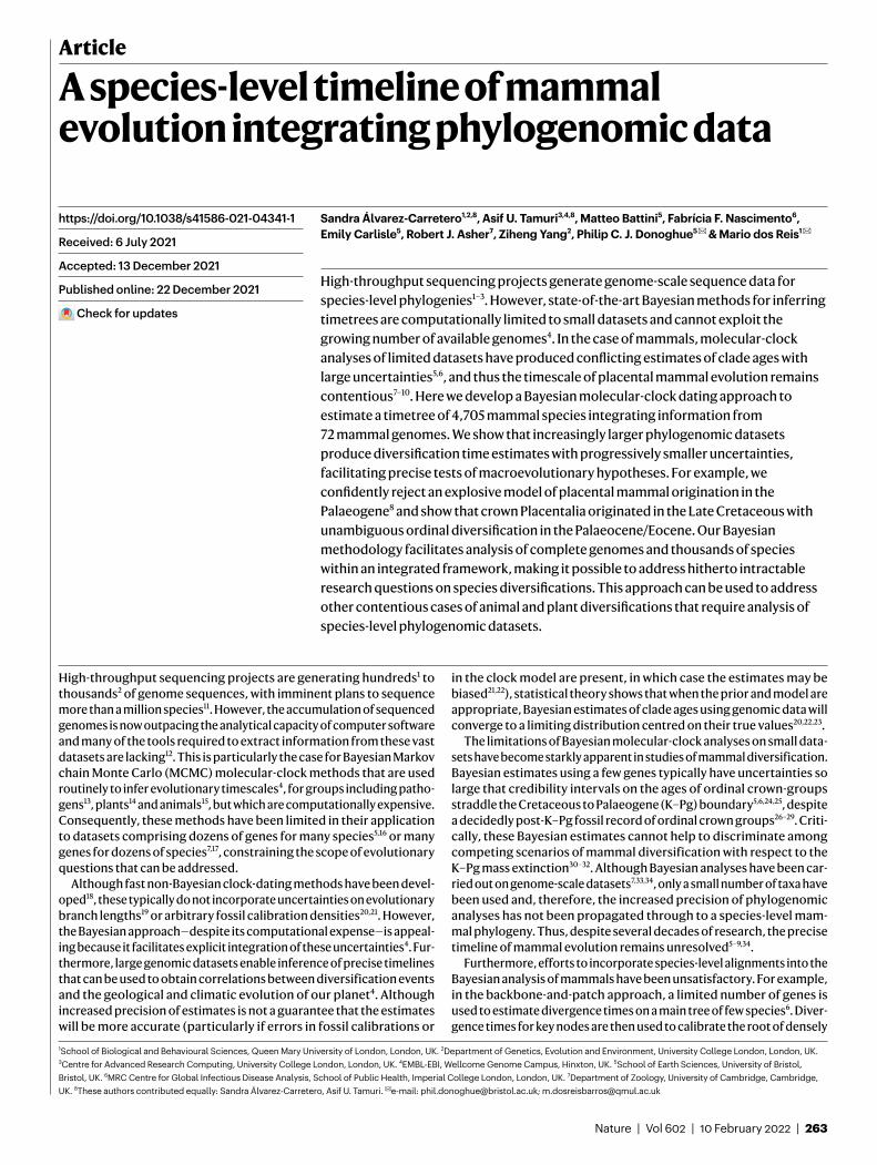
Sequential Bayesian dating of subtreesHere we overcome the limitations of previous Bayesian clock-dating studies on small datasets by developing the Bayesian sequential-subtree approach (Fig. 1), which we use to infer a timetree of 4,705 mammal spe-cies. First, a genome-scale alignment (15,268 one-to-one orthologues, 33.2 million aligned bases) and a suite of 32 fossil calibrations are used to infer the timetree for 72 species. The resulting posterior distribution of node ages is then used, together with a further set of 60 fossil calibrations, to date 13 subtrees encompassing 4,705 species with new alignments (182 loci, up to 5.33 × 105 aligned bases), thus avoiding data duplication in the likelihood (Methods). Our approach is feasible because we use the approximate likelihood calculation37, which provides a 1,000× speed-up over traditional MCMC timetree inference without loss of accuracy37,38. This facilitates analysis of more taxa and much longer alignments than has been possible previously (Table 1). By using the flexible skew-t and skew-normal distributions to model the posterior time estimates from the 72-genome analysis, we accurately transfer information from the genome-scale analysis into the subtree analysis35, augmented by the additional subtree-specific fossil calibrations. Our fossil calibrations restrict the minimum ages of clades on the basis of the oldest unequivocal

members of crown groups and, in most cases, also their maximum age through consideration of the presence and absence of stem and sister groups, their palaeoecology, palaeobiogeography and comparative taphonomy39 (Supplementary Information).

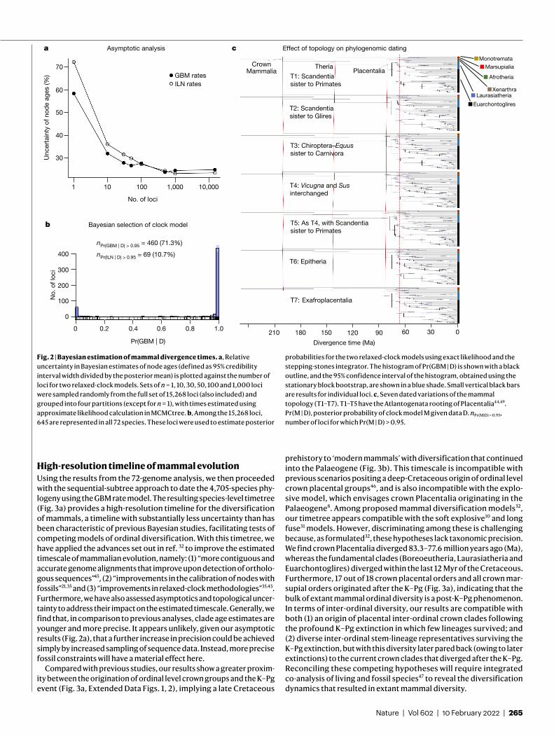
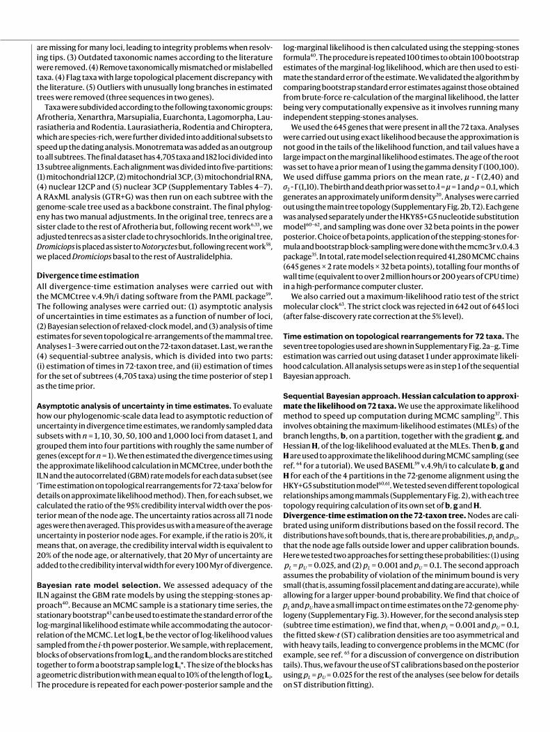
Analyses of small phylogenies36 and simulated data23,36 indicate that genome-scale data should lead to asymptotic reduction of uncertainty in divergence time estimates. We demonstrate this for our mammal data by performing random sampling of loci and calculating diver-gence times on the 72-species phylogeny. By increasing the number of loci analysed from 1 to 15,268, uncertainties in time estimates are progressively reduced irrespective of the relaxed-clock model used (Fig. 2a). Average relative uncertainty on node ages stabilizes at 23.6%–25.0% for the 15,268 loci. This means that, for each 1 million years (Myr) of divergence, approximately 250 thousand years (Kyr) of uncertainty is added to the width of the credibility intervals, which is substantially less than previous Bayesian analyses based on a limited number of genes5,6 (Table 1). Although reduction in uncertainty is modest beyond 1,000 loci (Fig. 2a), the analysis of the full dataset comes with little extra computational cost because the approximate likelihood calculation depends on the number of taxa, and not on the alignment length37.

We next assessed the fit of the relaxed-clock models by using the stepping-stones integrator40. This is critical because the competing autocorrelated (geometric Brownian motion23,41 (GBM)) and independ-ent log-normal23,42 (ILN) rate models can produce markedly different time estimates when using the same fossil calibrations35. Clock-model testing has not previously been conducted at large scale because mar-ginal likelihood inference requires expensive exact likelihood calcu-lation. We overcame this problem by implementing stationary block resampling43 to obtain reliable estimates of the standard error of the log-marginal likelihood estimates. In this way, we can guarantee the MCMC sample is large enough to obtain an acceptable error for cal-culating the posterior probabilities of the clock models. We find that, for 71.3% of the 645 loci analysed (Fig. 2b), GBM has a posterior prob-ability above 95%, whereas ILN has a posterior probability above 95% for only 10.7% of loci.

Some topological relationships among major groups of mammals—such as the placement of the placental root, the position of Scandentia with respect to Primates and Glires, and the position of several major groups within Laurasiatheria (Carnivora, Perissodactyla, Chiroptera and Artiodactyla)—have been difficult to resolve32,33,44. We selected 7 re-arrangements of these major groups and estimated the divergence times using the 15,268 loci and the 72-species phylogeny. We find these topological re-arrangements have a marginal effect on estimated diver-gence times (Fig. 2c), apparently because these topological uncertain-ties are characterized by small internal branches.

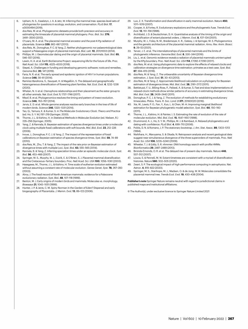
Use HMMpro�les toextend orthologyto 4,705 taxa

Divide 4,705-taxon treeinto 13subtrees

Estimatetimes on 13species-levelsubtreesusing �ttedST/SN as prior

Joinsubtrees toassemble4,705-taxontimetree

Estimatetimes on72-taxontree

Fit ST and SNdensities to72-taxonposterior

Ensemblmining oforthologues in72 genomes

Fig. 1 | Summary of the Bayesian sequential subtree dating approach. The pipeline is divided into molecular data preparation (blue), dating step 1 (green) and dating step 2 (red). The number of taxa ranges from 10 to 72 among genomic loci (50% of loci are present in at least 67 taxa and 90% are present in at least 53 taxa), and from 48 to 3,986 in the 182 gene set. A hidden Markov model45 (HMM) was used to detect homology and construct the subtree alignments, thus bypassing unreliable homology annotations (Methods). SN, skew-normal distribution; ST, skew-t distribution.

Table 1 | Comparison of molecular-clock dating studies of mammal divergences

Study Taxa in molecular alignmenta

Genesb Alignment lengthc Estimated age of crown Mammaliad (Ma)

Estimated age of Placentaliad (Ma)

No. of placental crown orders originating in K (Pg)

Ref. 46 2,182 66 51,089 166.2 (fixed) 108.7–93.9 9 (7)

Ref. 5 164 26 35,603 238.2–203.3 116.8–92.1 7 (10)

Ref. 7 274 (36) 12 (14,632) 7,370 (20.6 × 10 6) 191.9–174.1 90.4–87.9 2 (10)

Ref. 8 46 27 36,860 167.7–164.7 64.85 (fixed) 0 (14)

Ref. 6 4,098 31 39,099 210.9–166.7 105.0–77.4 9 (9)

This study 4,705 (72) 182 (15,268) > 104 (33.2 × 10 6) 251–165 83.3–77.6 1 (17)aNumbers in parentheses show the number of complete genomes in the alignment. bNumbers in parentheses show the number of genes in the genome-scale part of the alignment. cNumbers in parentheses are the number of nucleotide sites in the genome-scale part of the alignment. In this study, subtree alignment lengths range from 5.11 × 104 to 5.33 × 105 bases. Missing data range from 46% to 60% in the genomic partitions and from 17% to 99% in the subtree partitions (Methods). dGiven as the 95% credibility (for Bayesian studies) or confidence (for non-Bayesian studies) interval. Studies using Bayesian analysis are shown in bold. K, Cretaceous; Pg, Palaeogene.

Nature | Vol 602 | 10 February 2022 | 265

b

a

nPr(GBM | D) > 0.95 = 460 (71.3%)

nPr(ILN | D) > 0.95 = 69 (10.7%)

c Effect of topology on phylogenomic dating

0306090120150180210

T1: Scandentia sister to Primates

T2: Scandentiasister to Glires

T3: Chiroptera–Equussister to Carnivora

T4: Vicugna and Susinterchanged

T5: As T4, with Scandentiasister to Primates

T6: Epitheria

T7: Exafroplacentalia

Asymptotic analysis

GBM ratesILN rates

60

50

40

30

70

Unc

erta

inty

of n

ode

ages

(%)

1 10 100 1,000 10,000

No. of loci

Bayesian selection of clock model

No.

of l

oci

400

300

200

100

0

Pr(GBM | D)

0 0.2 0.4 0.6 0.8 1.0

Divergence time (Ma)

CrownMammalia

TheriaPlacentalia

Euarchontoglires

LaurasiatheriaXenarthra

Afrotheria

Marsupialia

Monotremata

Fig. 2 | Bayesian estimation of mammal divergence times. a, Relative uncertainty in Bayesian estimates of node ages (defined as 95% credibility interval width divided by the posterior mean) is plotted against the number of loci for two relaxed-clock models. Sets of n = 1, 10, 30, 50, 100 and 1,000 loci were sampled randomly from the full set of 15,268 loci (also included) and grouped into four partitions (except for n = 1), with times estimated using approximate likelihood calculation in MCMCtree. b, Among the 15,268 loci, 645 are represented in all 72 species. These loci were used to estimate posterior

probabilities for the two relaxed-clock models using exact likelihood and the stepping-stones integrator. The histogram of Pr(GBM | D) is shown with a black outline, and the 95% confidence interval of the histogram, obtained using the stationary block bootstrap, are shown in a blue shade. Small vertical black bars are results for individual loci. c, Seven dated variations of the mammal topology (T1–T7). T1–T5 have the Atlantogenata rooting of Placentalia44,49. Pr(M | D), posterior probability of clock model M given data D. nPr(M|D) > 0.95, number of loci for which Pr(M | D) > 0.95.

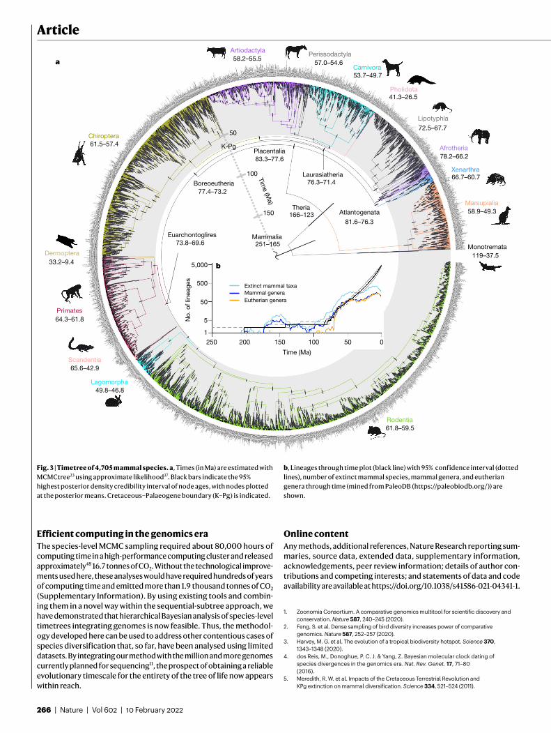
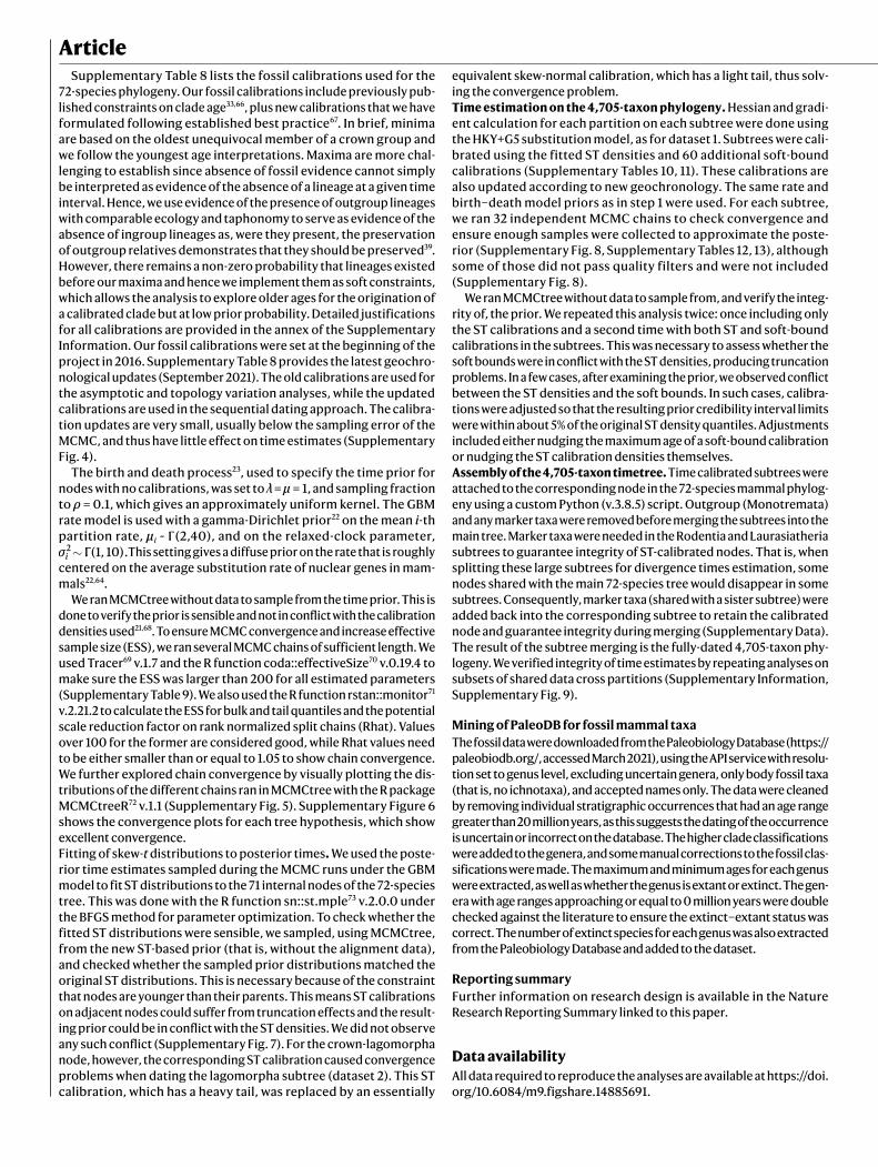
High-resolution timeline of mammal evolutionUsing the results from the 72-genome analysis, we then proceeded with the sequential-subtree approach to date the 4,705-species phy-logeny using the GBM rate model. The resulting species-level timetree (Fig. 3a) provides a high-resolution timeline for the diversification of mammals, a timeline with substantially less uncertainty than has been characteristic of previous Bayesian studies, facilitating tests of competing models of ordinal diversification. With this timetree, we have applied the advances set out in ref. 32 to improve the estimated timescale of mammalian evolution, namely: (1) “more contiguous and accurate genome alignments that improve upon detection of ortholo-gous sequences”45, (2) “improvements in the calibration of nodes with fossils”21,35 and (3) “improvements in relaxed-clock methodologies”35,43. Furthermore, we have also assessed asymptotics and topological uncer-tainty to address their impact on the estimated timescale. Generally, we find that, in comparison to previous analyses, clade age estimates are younger and more precise. It appears unlikely, given our asymptotic results (Fig. 2a), that a further increase in precision could be achieved simply by increased sampling of sequence data. Instead, more precise fossil constraints will have a material effect here.

Compared with previous studies, our results show a greater proxim-ity between the origination of ordinal level crown groups and the K–Pg event (Fig. 3a, Extended Data Figs. 1, 2), implying a late Cretaceous

prehistory to ‘modern mammals’ with diversification that continued into the Palaeogene (Fig. 3b). This timescale is incompatible with previous scenarios positing a deep-Cretaceous origin of ordinal level crown placental groups46, and is also incompatible with the explo-sive model, which envisages crown Placentalia originating in the Palaeogene8. Among proposed mammal diversification models32, our timetree appears compatible with the soft explosive10 and long fuse31 models. However, discriminating among these is challenging because, as formulated32, these hypotheses lack taxonomic precision. We find crown Placentalia diverged 83.3–77.6 million years ago (Ma), whereas the fundamental clades (Boreoeutheria, Laurasiatheria and Euarchontoglires) diverged within the last 12 Myr of the Cretaceous. Furthermore, 17 out of 18 crown placental orders and all crown mar-supial orders originated after the K–Pg (Fig. 3a), indicating that the bulk of extant mammal ordinal diversity is a post-K–Pg phenomenon. In terms of inter-ordinal diversity, our results are compatible with both (1) an origin of placental inter-ordinal crown clades following the profound K–Pg extinction in which few lineages survived; and (2) diverse inter-ordinal stem-lineage representatives surviving the K–Pg extinction, but with this diversity later pared back (owing to later extinctions) to the current crown clades that diverged after the K–Pg. Reconciling these competing hypotheses will require integrated co-analysis of living and fossil species47 to reveal the diversification dynamics that resulted in extant mammal diversity.

266 | Nature | Vol 602 | 10 February 2022

Article

Efficient computing in the genomics eraThe species-level MCMC sampling required about 80,000 hours of computing time in a high-performance computing cluster and released approximately48 16.7 tonnes of CO2. Without the technological improve-ments used here, these analyses would have required hundreds of years of computing time and emitted more than 1.9 thousand tonnes of CO2 (Supplementary Information). By using existing tools and combin-ing them in a novel way within the sequential-subtree approach, we have demonstrated that hierarchical Bayesian analysis of species-level timetrees integrating genomes is now feasible. Thus, the methodol-ogy developed here can be used to address other contentious cases of species diversification that, so far, have been analysed using limited datasets. By integrating our method with the million and more genomes currently planned for sequencing11, the prospect of obtaining a reliable evolutionary timescale for the entirety of the tree of life now appears within reach.

Online contentAny methods, additional references, Nature Research reporting sum-maries, source data, extended data, supplementary information, acknowledgements, peer review information; details of author con-tributions and competing interests; and statements of data and code availability are available at https://doi.org/10.1038/s41586-021-04341-1.

1. Zoonomia Consortium. A comparative genomics multitool for scientific discovery and conservation. Nature 587, 240–245 (2020).

2. Feng, S. et al. Dense sampling of bird diversity increases power of comparative genomics. Nature 587, 252–257 (2020).

3. Harvey, M. G. et al. The evolution of a tropical biodiversity hotspot. Science 370, 1343–1348 (2020).

4. dos Reis, M., Donoghue, P. C. J. & Yang, Z. Bayesian molecular clock dating of species divergences in the genomics era. Nat. Rev. Genet. 17, 71–80 (2016).

5. Meredith, R. W. et al. Impacts of the Cretaceous Terrestrial Revolution and KPg extinction on mammal diversification. Science 334, 521–524 (2011).

Marsupialia58.9–49.3

Xenarthra66.7–60.7

Chiroptera61.5–57.4

Artiodactyla58.2–55.5

Scandentia65.6–42.9

Dermoptera33.2–9.4

Monotremata119–37.5

Theria166–123

Placentalia83.3–77.6

Boreoeutheria77.4–73.2

Atlantogenata

81.6–76.3

Lipotyphla

72.5–67.7

Afrotheria78.2–66.2

Carnivora53.7–49.7

Perissodactyla57.0–54.6

Primates64.3–61.8

Rodentia61.8–59.5

Lagomorpha49.8–46.8

a

Mammalia251–165

Euarchontoglires73.8–69.6

Laurasiatheria76.3–71.4

Pholidota41.3–26.5

Time

(Ma)

50

100

150

K-Pg

5,000

500

50

5

b

1

No.

of l

inea

ges

Extinct mammal taxaMammal generaEutherian genera

250 200 150 100

Time (Ma)

50 0

Fig. 3 | Timetree of 4,705 mammal species. a, Times (in Ma) are estimated with MCMCtree23 using approximate likelihood37. Black bars indicate the 95% highest posterior density credibility interval of node ages, with nodes plotted at the posterior means. Cretaceous–Palaeogene boundary (K–Pg) is indicated.

b, Lineages through time plot (black line) with 95%  confidence interval (dotted lines), number of extinct mammal species, mammal genera, and eutherian genera through time (mined from PaleoDB (https://paleobiodb.org/)) are shown.

Nature | Vol 602 | 10 February 2022 | 267

6. Upham, N. S., Esselstyn, J. A. & Jetz, W. Inferring the mammal tree: species-level sets of phylogenies for questions in ecology, evolution, and conservation. PLoS Biol. 17, e3000494 (2019).

7. dos Reis, M. et al. Phylogenomic datasets provide both precision and accuracy in estimating the timescale of placental mammal phylogeny. Proc. Biol. Sci. 279, 3491–3500 (2012).

8. O’Leary, M. A. et al. The placental mammal ancestor and the post-K-Pg radiation of placentals. Science 339, 662–667 (2013).

9. dos Reis, M., Donoghue, P. C. & Yang, Z. Neither phylogenomic nor palaeontological data support a Palaeogene origin of placental mammals. Biol. Lett. 10, 20131003 (2014).

10. Phillips, M. J. Geomolecular dating and the origin of placental mammals. Syst. Biol. 65, 546–557 (2016).

11. Lewin, H. A. et al. Earth BioGenome Project: sequencing life for the future of life. Proc. Natl Acad. Sci. USA 115, 4325–4333 (2018).

12. Siepel, A. Challenges in funding and developing genomic software: roots and remedies. Genome Biol. 20, 147 (2019).

13. Faria, N. R. et al. The early spread and epidemic ignition of HIV-1 in human populations. Science 346, 56–61 (2014).

14. Ramírez-Barahona, S., Sauquet, H. & Magallón, S. The delayed and geographically heterogeneous diversification of flowering plant families. Nat. Ecol. Evol. 4, 1232–1238 (2020).

15. Whelan, N. V. et al. Ctenophore relationships and their placement as the sister group to all other animals. Nat. Ecol. Evol. 1, 1737–1746 (2017).

16. Misof, B. et al. Phylogenomics resolves the timing and pattern of insect evolution. Science 346, 763–767 (2014).

17. Jarvis, E. D. et al. Whole-genome analyses resolve early branches in the tree of life of modern birds. Science 346, 1320–1331 (2014).

18. Tao, Q., Tamura, K. & Kumar, S. in The Molecular Evolutionary Clock: Theory and Practice (ed. Ho, S. Y. W.) 197–219 (Springer, 2020).

19. Thorne, J. L. & Kishino, H. in Statistical Methods in Molecular Evolution (ed. Nielsen, R.) 235–256 (Springer, 2005).

20. Yang, Z. & Rannala, B. Bayesian estimation of species divergence times under a molecular clock using multiple fossil calibrations with soft bounds. Mol. Biol. Evol. 23, 212–226 (2006).

21. Inoue, J., Donoghue, P. C. J. & Yang, Z. The impact of the representation of fossil calibrations on Bayesian estimation of species divergence times. Syst. Biol. 59, 74–89 (2010).

22. dos Reis, M., Zhu, T. & Yang, Z. The impact of the rate prior on Bayesian estimation of divergence times with multiple Loci. Syst. Biol. 63, 555–565 (2014).

23. Rannala, B. & Yang, Z. Inferring speciation times under an episodic molecular clock. Syst. Biol. 56, 453–466 (2007).

24. Springer, M. S., Murphy, W. J., Eizirik, E. & O’Brien, S. J. Placental mammal diversification and the Cretaceous–Tertiary boundary. Proc. Natl Acad. Sci. USA 100, 1056–1061 (2003).

25. Hasegawa, M., Thorne, J. L. & Kishino, H. Time scale of eutherian evolution estimated without assuming a constant rate of molecular evolution. Genes Genet. Syst. 78, 267–283 (2003).

26. Alroy, J. The fossil record of North American mammals: evidence for a Paleocene evolutionary radiation. Syst. Biol. 48, 107–118 (1999).

27. Benton, M. J. Early origins of modern birds and mammals: Molecules vs. morphology. Bioessays 21, 1043–1051 (1999).

28. Hunter, J. P. & Janis, C. M. Spiny Norman in the Garden of Eden? Dispersal and early biogeography of Placentalia. J. Mamm. Evol. 13, 89–123 (2006).

29. Luo, Z. X. Transformation and diversification in early mammal evolution. Nature 450, 1011–1019 (2007).

30. Cooper, A. & Fortey, R. Evolutionary explosions and the phylogenetic fuse. Trends Ecol. Evol. 13, 151–156 (1998).

31. Archibald, J. D. & Deutschman, D. H. Quantitative analysis of the timing of the origin and diversification of extant placental orders. J. Mamm. Evol. 8, 107–124 (2001).

32. Murphy, W. J., Foley, N. M., Bredemeyer, K. R., Gatesy, J. & Springer, M. S. Phylogenomics and the genetic architecture of the placental mammal radiation. Annu. Rev. Anim. Biosci. 9, 29–53 (2021).

33. Tarver, J. E. et al. The interrelationships of placental mammals and the limits of phylogenetic inference. Genome Biol. Evol. 8, 330–344 (2016).

34. Liu, L. et al. Genomic evidence reveals a radiation of placental mammals uninterrupted by the KPg boundary. Proc. Natl Acad. Sci. USA 114, E7282–E7290 (2017).

35. dos Reis, M. et al. Using phylogenomic data to explore the effects of relaxed clocks and calibration strategies on divergence time estimation: primates as a test case. Syst. Biol. 67, 594–615 (2018).

36. dos Reis, M. & Yang, Z. The unbearable uncertainty of Bayesian divergence time estimation. J. Syst. Evol. 51, 30–43 (2013).

37. dos Reis, M. & Yang, Z. Approximate likelihood calculation on a phylogeny for Bayesian estimation of divergence times. Mol. Biol. Evol. 28, 2161–2172 (2011).

38. Battistuzzi, F. U., Billing-Ross, P., Paliwal, A. & Kumar, S. Fast and slow implementations of relaxed-clock methods show similar patterns of accuracy in estimating divergence times. Mol. Biol. Evol. 28, 2439–2442 (2011).

39. Donoghue, P. C. J. & Yang, Z. The evolution of methods for establishing evolutionary timescales. Philos. Trans. R. Soc. Lond. B 371, 20160020 (2016).

40. Xie, W., Lewis, P. O., Fan, Y., Kuo, L. & Chen, M.-H. Improving marginal likelihood estimation for Bayesian phylogenetic model selection. Syst. Biol. 60, 150–160 (2011).

41. Thorne, J. L., Kishino, H. & Painter, I. S. Estimating the rate of evolution of the rate of molecular evolution. Mol. Biol. Evol. 15, 1647–1657 (1998).

42. Drummond, A. J., Ho, S. Y. W., Phillips, M. J. & Rambaut, A. Relaxed phylogenetics and dating with confidence. PLoS Biol. 4, 699–710 (2006).

43. Politis, D. N. & Romano, J. P. The stationary bootstrap. J. Am. Stat. Assoc. 89, 1303–1313 (1994).

44. Nishihara, H., Maruyama, S. & Okada, N. Retroposon analysis and recent geological data suggest near-simultaneous divergence of the three superorders of mammals. Proc. Natl Acad. Sci. USA 106, 5235–5240 (2009).

45. Wheeler, T. J. & Eddy, S. R. nhmmer: DNA homology search with profile HMMs. Bioinformatics 29, 2487–2489 (2013).

46. Bininda-Emonds, O. R. et al. The delayed rise of present-day mammals. Nature 446, 507–512 (2007).

47. Louca, S. & Pennell, M. W. Extant timetrees are consistent with a myriad of diversification histories. Nature 580, 502–505 (2020).

48. Zwart, S. P. The ecological impact of high-performance computing in astrophysics. Nat. Astron. 4, 819–822 (2020).

49. Springer, M. S., Stanhope, M. J., Madsen, O. & de Jong, W. W. Molecules consolidate the placental mammal tree. Trends Ecol. Evol. 19, 430–438 (2004).

Publisher’s note Springer Nature remains neutral with regard to jurisdictional claims in published maps and institutional affiliations.

© The Author(s), under exclusive licence to Springer Nature Limited 2021

ArticleMethods

Data collection and filteringDataset 1: 72-genome alignment. We downloaded the set of one-to-one protein-coding orthologues for the 72 mammal genomes available in Ensembl release 98 (http://www.ensembl.org, accessed 15 November 2019) using EnsemblBioMarts50 (https://m.ensembl.org/biomart/martview). Sequences that did not meet the following requirements were removed from further analysis: (1) present in both human and mouse, (2) not containing internal stop codons or gene/transcript mismatches, (3) present in at least 10 species, and (4) at least 100 codons in length. This left a total of 15,569 orthologues, which we partitioned into two data blocks: (1) first and second codon posi-tions (12CP) and (2) third codon positions (3CP). For each orthologue, an alignment was built with PRANK v.14060351 and the best-scoring maximum-likelihood (ML) trees were inferred with RAxML v.8.2.1052. We used only the alignments with the 12CP-partition in the subsequent Bayesian molecular-clock analyses.

We further filtered the dataset using the estimated best-scoring ML trees for each gene to identify those having a branch length larger than 60% of the total tree length (the sum of all branch lengths). The rela-tive branch length test is useful to detect misaligned or misidentified orthologues in the alignments7,53, which may result in unusually long branch lengths. Let bij be the i-th branch length for gene tree j, and let n be the number of branches in the tree, then the relative branch length is

∑r b b= / . (1)ij iji

n

ij=1

We identified 133 orthologue alignments associated with at least one relative branch length larger than 60%. These orthologue alignments were removed from further analyses.

Then, we estimated the pairwise distance between each orthologue in Mus musculus and Homo sapiens using the R (v.3.5 to v.4.0) func-tion ape::dist.dna54 v.5.5. There were 4 genes (ENSG00000132185, ENSG00000204544, ENSG00000120937 and ENSG00000236699) for which the distances were returned as NaN for at least one of the substitution models used (TN93 and JC69) or larger than 0.75 for the raw distance. Furthermore, when we plotted the percentage of the tree length inferred for each orthologue alignment versus the cor-responding largest branch length (also as percentage), we found an outlier (ENSG00000176973; Supplementary Fig. 1). We removed these 5 orthologue alignments, resulting in 15,431 orthologous gene align-ments. Of those, 163 orthologues were removed as they are used in the construction of dataset 2 (see below). This filtering step resulted in 15,268 orthologue alignments (Supplementary Table 1).

The 15,268 orthologue alignments were sorted from fast- to slow-evolving according to the pairwise-distance estimates and grouped into four partitions with the same number of genes. Each of the four partitions contained the concatenated 12CP of the orthologues for the partition (Supplementary Table 2). The rationale for this partition-ing strategy is as follows. In previous work7,55, we tested phylogenomic data partitioning according to locus rate, principal component analysis of relative branch lengths and amino acid composition at loci. However, those analyses showed no noticeable differences in posterior time esti-mates across the partitioning strategies7,55. Conversely, we have shown that uncertainty in time estimates is sensitive to the number of parti-tions used7,22, with more partitions producing more precise estimates, but at the cost of additional computation time. It appears that four partitions give a reasonable trade-off between computational speed and precision of estimates. For example, 20 partitions would produce slightly more precise estimates but at 5 times the computational cost.

Dataset 2: alignments of 4,705 taxa. We downloaded 832 com-plete mammal mitochondrial genomes from NCBI RefSeq (accessed

14 January 2016). Twelve extinct and 2 redundant entries were removed, leaving 818 genomes. Twelve protein-coding genes (all but ND6) and the two non-coding RNA genes were extracted from each genome. The overlapping region in ATP8 (position 95 to end) and overlapping codons at the end of ND4L were deleted.

To increase the nuclear and mitochondrial datasets, we mined sequences deposited in the European Nucleotide Archive (ENA; https://www.ebi.ac.uk/ena). The GenBank taxonomy (ftp://ftp.ncbi.nih.gov/pub/taxonomy/) was used to search for non-Ensembl mammalia spe-cies (this taxonomy is only used for ENA searches and not for any other analyses). A total of 7,188 taxa were found, 83 of which were extinct. The GenBank identifiers were used to reference the corresponding taxa in the ENA, from which all matching coding and non-coding sequences for non-Ensembl mammal taxa were downloaded (accessed 17 January 2016): we found 6,453 taxa with coding sequences and 3,239 taxa with non-coding sequences (6,606 distinct taxa).

This project started in early 2016. At the time, we downloaded 15,904 nuclear orthologous gene alignments for 43 mammal taxa from Ensembl 83 and used these orthologues to create HMM sequence profiles with HMMER56. The HMM profiles were then used to identify orthologues for additional taxa from GenBank (https://www.ncbi.nlm.nih.gov/genbank/), bypassing unreliable GenBank homology annota-tions, and thus allowing reliable construction of large mammal sub-trees. In late 2019, we updated the 15,904 orthologues to 72 genomes using Ensembl 98, but the HMM profiles and corresponding homology searches were based on the 2016 mining of Ensembl. HMM profiles were also created for mitochondrial protein-coding and non-coding genes and used for taxa extension of the corresponding alignments. DNA homology searches were performed with nhmmer45 using the following match criteria: (1) sequences with E-value < 10−100 for a single gene were collected (that is, sequences with multiple low E-values for different genes were removed); (2) matched sequences had to be at least 70% as long as the shortest Ensembl sequence in the alignment because many deposited sequences are partial sequences; (3) matches from hybrid and cross species were removed; (4) unspecified species were excluded, unless no other member of the genus was represented (4 taxa included); (5) unconfirmed species were excluded, unless no other member of the genus was represented (1 taxon included); and (6) coding sequences were checked for correct open reading frame and translation.

Nuclear genes resulting in an expanded set of at least 50 taxa were selected, resulting in a set of 168 nuclear genes. These 168 genes cor-respond to 163 genes in the 2019 Ensembl mining (5 genes did not pass filtering criteria for the 72 taxa, but they did pass the criteria with the 43 taxa). Thus dataset 1, based on the 2019 Ensembl mining, was reduced from 15,431 genes to 15,268 (Supplementary Table 1) to avoid data dupli-cation in the sequential dating approach. For new mined taxa, sequence annotations were extracted, sorted, and visually inspected to help ver-ify homology. Alignments were then extended with homology-matched sequences using PAGAN v.0.6157. Sequences were added in order of decreasing length (that is, longest sequences were added to the align-ment first). Supplementary Table 3 gives summaries of the numbers of taxa and alignment lengths for datasets 1 and 2.

We then used RAxML to estimate the topology for each one of the 182 loci (168 nuclear and 14 mitochondrial) under the GTR+G model. We then manually inspected the trees and further filtered taxa following these criteria: (1) remove taxa that did not share genes with their order, family, and genus. This is done to avoid unidentifiable positioning of taxa in the subtrees: if a species does not share genes with its close rela-tives, then several positionings of the species within the subtree will have the same likelihood (also known as ‘likelihood terraces’). (2) Keep only one member of each species while maintaining maximum locus coverage, that is, remove redundant subspecies. Many subspecies slow the analysis down and are not informative about deep divergences (for example, Rangifer tarandus tarandus). Also, subspecies annotations

are missing for many loci, leading to integrity problems when resolv-ing tips. (3) Outdated taxonomic names according to the literature were removed. (4) Remove taxonomically mismatched or mislabelled taxa. (4) Flag taxa with large topological placement discrepancy with the literature. (5) Outliers with unusually long branches in estimated trees were removed (three sequences in two genes).

Taxa were subdivided according to the following taxonomic groups: Afrotheria, Xenarthra, Marsupialia, Euarchonta, Lagomorpha, Lau-rasiatheria and Rodentia. Laurasiatheria, Rodentia and Chiroptera, which are species-rich, were further divided into additional subsets to speed up the dating analysis. Monotremata was added as an outgroup to all subtrees. The final dataset has 4,705 taxa and 182 loci divided into 13 subtree alignments. Each alignment was divided into five-partitions: (1) mitochondrial 12CP, (2) mitochondrial 3CP, (3) mitochondrial RNA, (4) nuclear 12CP and (5) nuclear 3CP (Supplementary Tables 4–7). A RAxML analysis (GTR+G) was then run on each subtree with the genome-scale tree used as a backbone constraint. The final phylog-eny has two manual adjustments. In the original tree, tenrecs are a sister clade to the rest of Afrotheria but, following recent work6,33, we adjusted tenrecs as a sister clade to chrysochlorids. In the original tree, Dromiciops is placed as sister to Notoryctes but, following recent work58, we placed Dromiciops basal to the rest of Australidelphia.

Divergence time estimationAll divergence-time estimation analyses were carried out with the MCMCtree v.4.9h/i dating software from the PAML package59. The following analyses were carried out: (1) asymptotic analysis of uncertainties in time estimates as a function of number of loci, (2) Bayesian selection of relaxed-clock model, and (3) analysis of time estimates for seven topological re-arrangements of the mammal tree. Analyses 1–3 were carried out on the 72-taxon dataset. Last, we ran the (4) sequential-subtree analysis, which is divided into two parts: (i) estimation of times in 72-taxon tree, and (ii) estimation of times for the set of subtrees (4,705 taxa) using the time posterior of step 1 as the time prior.

Asymptotic analysis of uncertainty in time estimates. To evaluate how our phylogenomic-scale data lead to asymptotic reduction of uncertainty in divergence time estimates, we randomly sampled data subsets with n = 1, 10, 30, 50, 100 and 1,000 loci from dataset 1, and grouped them into four partitions with roughly the same number of genes (except for n = 1). We then estimated the divergence times using the approximate likelihood calculation in MCMCtree, under both the ILN and the autocorrelated (GBM) rate models for each data subset (see ‘Time estimation on topological rearrangements for 72-taxa’ below for details on approximate likelihood method). Then, for each subset, we calculated the ratio of the 95% credibility interval width over the pos-terior mean of the node age. The uncertainty ratios across all 71 node ages were then averaged. This provides us with a measure of the average uncertainty in posterior node ages. For example, if the ratio is 20%, it means that, on average, the credibility interval width is equivalent to 20% of the node age, or alternatively, that 20 Myr of uncertainty are added to the credibility interval width for every 100 Myr of divergence.

Bayesian rate model selection. We assessed adequacy of the ILN against the GBM rate models by using the stepping-stones ap-proach40. Because an MCMC sample is a stationary time series, the stationary bootstrap43 can be used to estimate the standard error of the log-marginal likelihood estimate while accommodating the autocor-relation of the MCMC. Let log Li be the vector of log-likelihood values sampled from the i-th power posterior. We sample, with replacement, blocks of observations from log Li, and the random blocks are stitched together to form a bootstrap sample log Li*. The size of the blocks has a geometric distribution with mean equal to 10% of the length of log Li. The procedure is repeated for each power-posterior sample and the

log-marginal likelihood is then calculated using the stepping-stones formula40. The procedure is repeated 100 times to obtain 100 bootstrap estimates of the marginal-log likelihood, which are then used to esti-mate the standard error of the estimate. We validated the algorithm by comparing bootstrap standard error estimates against those obtained from brute-force re-calculation of the marginal likelihood, the latter being very computationally expensive as it involves running many independent stepping-stones analyses.

We used the 645 genes that were present in all the 72 taxa. Analyses were carried out using exact likelihood because the approximation is not good in the tails of the likelihood function, and tail values have a large impact on the marginal likelihood estimates. The age of the root was set to have a prior mean of 1 using the gamma density Γ(100,100). We used diffuse gamma priors on the mean rate, μ ~ Γ(2,40) and σ2 ~ Γ(1,10). The birth and death prior was set to λ = μ = 1 and ρ = 0.1, which generates an approximately uniform density20. Analyses were carried out using the main tree topology (Supplementary Fig. 2b, T2). Each gene was analysed separately under the HKY85+G5 nucleotide substitution model60–62, and sampling was done over 32 beta points in the power posterior. Choice of beta points, application of the stepping-stones for-mula and bootstrap block-sampling were done with the mcmc3r v.0.4.3 package35. In total, rate model selection required 41,280 MCMC chains (645 genes × 2 rate models × 32 beta points), totalling four months of wall time (equivalent to over 2 million hours or 200 years of CPU time) in a high-performance computer cluster.

We also carried out a maximum-likelihood ratio test of the strict molecular clock63. The strict clock was rejected in 642 out of 645 loci (after false-discovery rate correction at the 5% level).

Time estimation on topological rearrangements for 72 taxa. The seven tree topologies used are shown in Supplementary Fig. 2a–g. Time estimation was carried out using dataset 1 under approximate likeli-hood calculation. All analysis setups were as in step 1 of the sequential Bayesian approach.

Sequential Bayesian approach. Hessian calculation to approxi-mate the likelihood on 72 taxa. We use the approximate likelihood method to speed up computation during MCMC sampling37. This involves obtaining the maximum-likelihood estimates (MLEs) of the branch lengths, b, on a partition, together with the gradient g, and Hessian H, of the log-likelihood evaluated at the MLEs. Then b, g and H are used to approximate the likelihood during MCMC sampling (see ref. 64 for a tutorial). We used BASEML59 v.4.9h/i to calculate b, g and H for each of the 4 partitions in the 72-genome alignment using the HKY+G5 substitution model60,61. We tested seven different topological relationships among mammals (Supplementary Fig. 2), with each tree topology requiring calculation of its own set of b, g and H.Divergence-time estimation on the 72-taxon tree. Nodes are cali-brated using uniform distributions based on the fossil record. The distributions have soft bounds, that is, there are probabilities, pL and pU, that the node age falls outside lower and upper calibration bounds. Here we tested two approaches for setting these probabilities: (1) using pL = pU = 0.025, and (2) pL = 0.001 and pU = 0.1. The second approach assumes the probability of violation of the minimum bound is very small (that is, assuming fossil placement and dating are accurate), while allowing for a larger upper-bound probability. We find that choice of pL and pU have a small impact on time estimates on the 72-genome phy-logeny (Supplementary Fig. 3). However, for the second analysis step (subtree time estimation), we find that, when pL = 0.001 and pU = 0.1, the fitted skew-t (ST) calibration densities are too asymmetrical and with heavy tails, leading to convergence problems in the MCMC (for example, see ref. 65 for a discussion of convergence on distribution tails). Thus, we favour the use of ST calibrations based on the posterior using pL = pU = 0.025 for the rest of the analyses (see below for details on ST distribution fitting).

ArticleSupplementary Table 8 lists the fossil calibrations used for the

72-species phylogeny. Our fossil calibrations include previously pub-lished constraints on clade age33,66, plus new calibrations that we have formulated following established best practice67. In brief, minima are based on the oldest unequivocal member of a crown group and we follow the youngest age interpretations. Maxima are more chal-lenging to establish since absence of fossil evidence cannot simply be interpreted as evidence of the absence of a lineage at a given time interval. Hence, we use evidence of the presence of outgroup lineages with comparable ecology and taphonomy to serve as evidence of the absence of ingroup lineages as, were they present, the preservation of outgroup relatives demonstrates that they should be preserved39. However, there remains a non-zero probability that lineages existed before our maxima and hence we implement them as soft constraints, which allows the analysis to explore older ages for the origination of a calibrated clade but at low prior probability. Detailed justifications for all calibrations are provided in the annex of the Supplementary Information. Our fossil calibrations were set at the beginning of the project in 2016. Supplementary Table 8 provides the latest geochro-nological updates (September 2021). The old calibrations are used for the asymptotic and topology variation analyses, while the updated calibrations are used in the sequential dating approach. The calibra-tion updates are very small, usually below the sampling error of the MCMC, and thus have little effect on time estimates (Supplementary Fig. 4).

The birth and death process23, used to specify the time prior for nodes with no calibrations, was set to λ = μ = 1, and sampling fraction to ρ = 0.1, which gives an approximately uniform kernel. The GBM rate model is used with a gamma-Dirichlet prior22 on the mean i-th partition rate, μi ~ Γ(2,40), and on the relaxed-clock parameter, σ Γ(1, 10).i

2 ∼ This setting gives a diffuse prior on the rate that is roughly centered on the average substitution rate of nuclear genes in mam-mals22,64.

We ran MCMCtree without data to sample from the time prior. This is done to verify the prior is sensible and not in conflict with the calibration densities used21,68. To ensure MCMC convergence and increase effective sample size (ESS), we ran several MCMC chains of sufficient length. We used Tracer69 v.1.7 and the R function coda::effectiveSize70 v.0.19.4 to make sure the ESS was larger than 200 for all estimated parameters (Supplementary Table 9). We also used the R function rstan::monitor71 v.2.21.2 to calculate the ESS for bulk and tail quantiles and the potential scale reduction factor on rank normalized split chains (Rhat). Values over 100 for the former are considered good, while Rhat values need to be either smaller than or equal to 1.05 to show chain convergence. We further explored chain convergence by visually plotting the dis-tributions of the different chains ran in MCMCtree with the R package MCMCtreeR72 v.1.1 (Supplementary Fig. 5). Supplementary Figure 6 shows the convergence plots for each tree hypothesis, which show excellent convergence.Fitting of skew-t distributions to posterior times. We used the poste-rior time estimates sampled during the MCMC runs under the GBM model to fit ST distributions to the 71 internal nodes of the 72-species tree. This was done with the R function sn::st.mple73 v.2.0.0 under the BFGS method for parameter optimization. To check whether the fitted ST distributions were sensible, we sampled, using MCMCtree, from the new ST-based prior (that is, without the alignment data), and checked whether the sampled prior distributions matched the original ST distributions. This is necessary because of the constraint that nodes are younger than their parents. This means ST calibrations on adjacent nodes could suffer from truncation effects and the result-ing prior could be in conflict with the ST densities. We did not observe any such conflict (Supplementary Fig. 7). For the crown-lagomorpha node, however, the corresponding ST calibration caused convergence problems when dating the lagomorpha subtree (dataset 2). This ST calibration, which has a heavy tail, was replaced by an essentially

equivalent skew-normal calibration, which has a light tail, thus solv-ing the convergence problem.Time estimation on the 4,705-taxon phylogeny. Hessian and gradi-ent calculation for each partition on each subtree were done using the HKY+G5 substitution model, as for dataset 1. Subtrees were cali-brated using the fitted ST densities and 60 additional soft-bound calibrations (Supplementary Tables 10, 11). These calibrations are also updated according to new geochronology. The same rate and birth–death model priors as in step 1 were used. For each subtree, we ran 32 independent MCMC chains to check convergence and ensure enough samples were collected to approximate the poste-rior (Supplementary Fig. 8, Supplementary Tables 12, 13), although some of those did not pass quality filters and were not included (Supplementary Fig. 8).

We ran MCMCtree without data to sample from, and verify the integ-rity of, the prior. We repeated this analysis twice: once including only the ST calibrations and a second time with both ST and soft-bound calibrations in the subtrees. This was necessary to assess whether the soft bounds were in conflict with the ST densities, producing truncation problems. In a few cases, after examining the prior, we observed conflict between the ST densities and the soft bounds. In such cases, calibra-tions were adjusted so that the resulting prior credibility interval limits were within about 5% of the original ST density quantiles. Adjustments included either nudging the maximum age of a soft-bound calibration or nudging the ST calibration densities themselves.Assembly of the 4,705-taxon timetree. Time calibrated subtrees were attached to the corresponding node in the 72-species mammal phylog-eny using a custom Python (v.3.8.5) script. Outgroup (Monotremata) and any marker taxa were removed before merging the subtrees into the main tree. Marker taxa were needed in the Rodentia and Laurasiatheria subtrees to guarantee integrity of ST-calibrated nodes. That is, when splitting these large subtrees for divergence times estimation, some nodes shared with the main 72-species tree would disappear in some subtrees. Consequently, marker taxa (shared with a sister subtree) were added back into the corresponding subtree to retain the calibrated node and guarantee integrity during merging (Supplementary Data). The result of the subtree merging is the fully-dated 4,705-taxon phy-logeny. We verified integrity of time estimates by repeating analyses on subsets of shared data cross partitions (Supplementary Information, Supplementary Fig. 9).

Mining of PaleoDB for fossil mammal taxaThe fossil data were downloaded from the Paleobiology Database (https://paleobiodb.org/, accessed March 2021), using the API service with resolu-tion set to genus level, excluding uncertain genera, only body fossil taxa (that is, no ichnotaxa), and accepted names only. The data were cleaned by removing individual stratigraphic occurrences that had an age range greater than 20 million years, as this suggests the dating of the occurrence is uncertain or incorrect on the database. The higher clade classifications were added to the genera, and some manual corrections to the fossil clas-sifications were made. The maximum and minimum ages for each genus were extracted, as well as whether the genus is extant or extinct. The gen-era with age ranges approaching or equal to 0 million years were double checked against the literature to ensure the extinct–extant status was correct. The number of extinct species for each genus was also extracted from the Paleobiology Database and added to the dataset.

Reporting summaryFurther information on research design is available in the Nature Research Reporting Summary linked to this paper.

Data availabilityAll data required to reproduce the analyses are available at https://doi.org/10.6084/m9.figshare.14885691.

Code availabilityA repository containing instructions to reproduce the analyses is avail-able at http://github.com/sabifo4/mammals_dating and https://doi.org/10.5281/zenodo.5736629. The MCMCtree software and mcmc3r R package are freely available from http://abacus.gene.ucl.ac.uk/soft-ware/paml.html and https://github.com/dosreislab, respectively. 50. Kinsella, R. J. et al. Ensembl BioMarts: a hub for data retrieval across taxonomic space.

Database 2011, bar030 (2011).51. Löytynoja, A. Phylogeny-aware alignment with PRANK. Methods Mol. Biol. 1079, 155–170

(2014).52. Stamatakis, A. RAxML version 8: a tool for phylogenetic analysis and post-analysis of

large phylogenies. Bioinformatics 30, 1312–1313 (2014).53. Springer, M. S. & Gatesy, J. On the importance of homology in the age of phylogenomics.

Syst. Biodivers. 16, 210–228 (2018).54. Paradis, E., Claude, J. & Strimmer, K. APE: analyses of phylogenetics and evolution in R

language. Bioinformatics 20, 289–290 (2004).55. dos Reis, M. et al. Uncertainty in the timing of origin of animals and the limits of precision

in molecular timescales. Curr. Biol. 25, 2939–2950 (2015).56. Eddy, S. R. Profile hidden Markov models. Bioinformatics 14, 755–763 (1998).57. Löytynoja, A., Vilella, A. J. & Goldman, N. Accurate extension of multiple sequence

alignments using a phylogeny-aware graph algorithm. Bioinformatics 28, 1684–1691 (2012).

58. Mitchell, K. J. et al. Molecular phylogeny, biogeography, and habitat preference evolution of marsupials. Mol. Biol. Evol. 31, 2322–2330 (2014).

59. Yang, Z. PAML 4: phylogenetic analysis by maximum likelihood. Mol. Biol. Evol. 24, 1586–1591 (2007).

60. Hasegawa, M., Kishino, H. & Yano, T. Dating of the human-ape splitting by a molecular clock of mitochondrial DNA. J. Mol. Evol. 22, 160–174 (1985).

61. Hasegawa, M., Yano, T.-A. & Kishino, H. A new molecular clock of mitochondrial DNA and the evolution of hominoids. Proc. Japan Acad. B 60, 95–98 (1984).

62. Yang, Z. Maximum likelihood phylogenetic estimation from DNA sequences with variable rates over sites: approximate methods. J. Mol. Evol. 39, 306–314 (1994).

63. Felsenstein, J. Evolutionary trees from DNA sequences: a maximum likelihood approach. J. Mol. Evol. 17, 368–376 (1981).

64. dos Reis, M. & Yang, Z. in Evolutionary Genomics: Statistical and Computational Methods (ed. Anisimova, M.) 309–330 (Springer, 2019).

65. Rannala, B., Zhu, T. & Yang, Z. Tail paradox, partial identifiability, and influential priors in Bayesian branch length inference. Mol Biol Evol. 29, 325–335 (2012).

66. Benton, M. J. et al. Constraints on the timescale of animal evolutionary history. Palaeontol. Electron. 18, 1–106 (2015).

67. Parham, J. F. et al. Best practices for justifying fossil calibrations. Syst. Biol. 61, 346–359 (2012).

68. Warnock, R. C. M., Parham, J. F., Joyce, W. G., Lyson, T. R. & Donoghue, P. C. J. Calibration uncertainty in molecular dating analyses: there is no substitute for the prior evaluation of time priors. Proc. R. Soc. B 282, 20141013 (2015).

69. Rambaut, A., Drummond, A. J., Xie, D., Baele, G. & Suchard, M. A. Posterior summarization in Bayesian phylogenetics using Tracer 1.7. Syst. Biol. 67, 901–904 (2018).

70. Plummer, M., Best, N., Cowles, K. & Vines, K. CODA: convergence diagnosis and output analysis for MCMC. R News 6, 7–11 (2006).

71. RStan: the R interface to Stan. R package. https://mc-stan.org (Stan Development Team, 2020).

72. Puttick, M. N. MCMCtreeR: functions to prepare MCMCtree analyses and visualize posterior ages on trees. Bioinformatics 35, 5321–5322 (2019).

73. Azzalini, A. The R package ‘sn’: the skew-normal and related distributions such as the skew-t. http://azzalini.stat.unipd.it/SN/ (2019).

Acknowledgements We thank J. Gilbert and C. G. Faulkes for help with the Rodentia subtrees. This work used computing resources from Queen Mary’s Apocrita HPC and University College London Myriad HPC facilities. This work was supported by Biotechnology and Biological Sciences Research Council, UK, awards BB/T01282X/1, BB/T012951/1 and BB/T012773/1.

Author contributions M.d.R. conceived the work. M.d.R., Z.Y., P.C.J.D., S.Á.-C. and A.U.T. designed the analysis. S.Á.-C., A.U.T., R.J.A., P.C.J.D., M.B., E.C. and F.F.N. compiled, processed and verified the molecular and fossil data. S.Á.-C., A.U.T. and M.d.R. analysed the data. M.d.R. and P.C.J.D. wrote the paper with input from all authors.

Competing interests The authors declare no competing interests.

Additional informationSupplementary information The online version contains supplementary material available at https://doi.org/10.1038/s41586-021-04341-1.Correspondence and requests for materials should be addressed to Philip C. J. Donoghue or Mario dos Reis.Peer review information Nature thanks Olaf Bininda-Emonds, Xing-Xing Shen and the other, anonymous reviewers for their contribution to the peer review of this work.Reprints and permissions information is available at http://www.nature.com/reprints.

Article

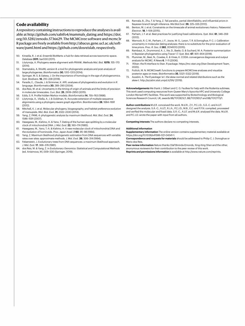
Extended Data Fig. 1 | Comparison of prior and posterior times. a, Prior distribution of node ages generated by MCMC sampling without the molecular alignment. b, Posterior distribution of node ages when the 72-genome

alignment is included during MCMC sampling. In both a and b, nodes are plotted at their posterior mean ages. The blue horizontal bars indicate the 95% credibility intervals of node ages.

Extended Data Fig. 2 | Impact of fossil calibration strategies on node age estimates. The posterior of node ages for the 72-taxon phylogeny is estimated using two additional fossil calibration strategies (y-axis) and plotted against the main estimates using best practice in calibration choice39 (x-axis). In all cases the fossil minima are the same, but the calibration maxima changes. In the first strategy (black dots), calibration densities are narrow and close to the fossil ages. A truncated-Cauchy with a short tail (using p = 0 and c = 0.001, which extends the tail to about 110% of the fossil age) is used21. This strategy assumes the fossil record is a good indicator of the true node ages. In the second

strategy (red dots), a truncated-Cauchy with a heavy tail (using p = 0.1 and c = 1, which extends the tail to over 900% of the fossil age) is used21. This strategy ignores the presence and absence of stem and sister groups, their palaeoecology, palaeobiogeography, and comparative taphonomy39; and instead, assumes the node ages can be arbitrarily old. Dots are plotted at the posterior mean ages and vertical and horizontal bars indicate 95% CIs. The solid line is the x = y line. The dashed lines are the regression lines for the corresponding data points.