A solution of the dichromatic model for multispectral photometric invariance

A Solution of the Dichromatic Model for Multispectral

Photometric Invariance

Cong Phuoc Huynh1 ∗ and Antonio Robles-Kelly1,2

1School of Engineering, Australian National University, Canberra ACT 0200, Australia

2National ICT Australia (NICTA) †, Locked Bag 8001, Canberra ACT 2601, Australia

Abstract

In this paper, we address the problem of photometric invariance in multispectral imaging

making use of an optimisation approach based upon the dichromatic model. In this manner,

we cast the problem of recovering the spectra of the illuminant, the surface reflectance and

the shading and specular factors in a structural optimisation setting. Making use of the addi-

tional information provided by multispectral imaging and the structure of image patches, we

recover the dichromatic parameters of the scene. To do this, we formulate a target cost func-

tion combining the dichromatic error and the smoothness priors for the surfaces under study.

The dichromatic parameters are recovered through minimising this cost function in a coor-

dinate descent manner. The algorithm is quite general in nature, admitting the enforcement

of smoothness constraints and extending in a straightforward manner to trichromatic settings.

Moreover, the objective function is convex with respect to the subset of variables to be op-

timised in each alternating step of the minimisation strategy. This gives rise to an optimal

closed-form solution for each of the iterations in our algorithm. We illustrate the effective-

ness of our method for purposes of illuminant spectrum recovery, skin recognition, material

clustering and specularity removal. We also compare our results to a number of alternatives.

Keywords: photometric invariance, multispectral imaging, dichromatic reflection model, re-

flectance.∗Corresponding author. E-mail: [email protected]. Tel: +61(2) 6267 6288†NICTA is funded by the Australian Government as represented by the Department of Broadband, Communications

and the Digital Economy and the Australian Research Council through the ICT Centre of Excellence program.

1

1 Introduction

In multispectral imaging, photometric invariants pose great opportunities and challenges in the

areas of shape analysis and material identification [14]. This is due to the information-rich rep-

resentation of the surface radiance acquired by multispectral and hyperspectral sensing devices,

which deliver wavelength-indexed data in thousands of bands across a broad spectrum. Ground-

based hyperspectral and multispectral imaging platforms, such as the Hyperspectral Image Inten-

sified Camera System 1 of OKSI, have recently become more commercially available. The advent

of these commercial systems opens up opportunities for applications in areas such as material and

object recognition and detection, biosecurity and surveillance. The ability to represent illumination

and surface reflectance as a spectral signature allows greater accuracy and flexibility to interpret

and distinguish colours than traditional trichromatic imagery. This is due to the robustness of

spectral signatures to metamerism, i.e. trichromatic matches between materials which may be very

different. In addition, hyperspectral imaging has been identified as a future direction in Compu-

tational Photography to reveal chemical or biological features for rendering and to provide high

quality archival imaging [47].

Moreover, in computer vision, the modelling of surface reflectance is a topic of pivotal impor-

tance for purposes of surface analysis and image understanding. For instance, Nayar and Bolle

[42] have used photometric invariants to recognise objects with different reflectance properties.

This work builds on the one reported in [43], where a background to foreground reflectance ratio is

introduced. In a related development, Dror et al. [16] have shown how surfaces may be classified

from single images through the use of reflectance properties. Moreover, although shape-from-

shading usually relies on the assumption of Lambertian reflectance [29], photometric correction or

specularity subtraction may be applied as a preprocessing step to improve the results obtained.

The main bulk of work concentrates on the effects encountered on shiny or rough surfaces. For

shiny surfaces, there are specular spikes and lobes which must be modelled. There have been

several attempts to remove specularities from images of non-Lambertian objects. For instance

Brelstaff and Blake [10] used a thresholding strategy to identify specularities on moving curved

objects. Narasimhan et al. [41] have formulated a scene radiance model for the class of “separa-

ble” Bidirectional Reflectance Distribution Functions (BRDFs), which can be used to separate the

model into material, object shape and lighting terms. More recently, Zickler et al. [61] introduced a

1For more information, see http://www.techexpo.com/WWW/opto-knowledge/prodhiicsi.html

2

method for transforming the original RGB colour space into an illuminant-dependent colour space

to obtain photometric invariants. Despite being effective, the application of these methods to mul-

tispectral imagery is somewhat limited since they are either constrained to trichromatic imagery or

rely on the closed form of the Bidirectional Reflectance Distribution Function (BRDF).

Moreover, other alternatives elsewhere in the literature aiming at detecting and removing specu-

larities either make use of additional hardware [42], impose constraints on the input images [39] or

require colour segmentation [32]. Hence, they are not readily applicable to multispectral images,

as there can be tens or even hundreds of bands for each pixel. Thus, any local operations, pre or

postprocessing must be exercised with caution and in relation to neighbouring spectral bands so as

to prevent spectral signature variation.

Specific to multispectral imagery, Healey and co-workers [25, 50, 52] have addressed the prob-

lem of photometric invariance for material classification and mapping in aerial imaging as related

to photometric artifacts induced by atmospheric effects and changing solar illumination. In [51],

a method is presented for hyperspectral edge detection. The method is robust to photometric ef-

fects, such as shadows and specularities. In [1], a photometrically invariant approach was proposed

based on the derivative analysis of the spectra. This local analysis of the spectra is intrinsic to the

surface albedo. Nonetheless, the analysis in [1] was derived from the Lambertian reflection model

and, hence, its not applicable to specular reflections. In [2], the same author derived a method to

detect specular highlights in multispectral images by making use of the spectral derivative of the

Fresnel reflection coefficient.

Since the recovery of illuminant and material reflectance are mutually interdependent, the prob-

lem here is closely related to colour constancy. Colour constancy is the ability to resolve the intrin-

sic material reflectance from their trichromatic colour images captured under varying illumination

conditions. The research on colour constancy branches in two main trends, one of them relies

on the statistics of illuminant and material reflectance, the other is drawn upon the physics-based

analysis of local shading and specularity of the surface material.

In the statistics-based approaches, the colour of input images is often correlated against a col-

lection of known illuminant chromaticities, such as those of Planckian light sources or black-body

radiators. A few of these employ Bayes’s rule [8, 9] to compute the best estimate from a posterior

distribution by standard methods such as maximum a posteriori (MAP), minimum-mean-squared

error (MMSE) or maximum local mass (MLM) estimation. The illuminant and surface reflectance

spectra typically take the form of a finite linear model with a Gaussian basis. A well-known in-

3

stance of this category is the Colour by Correlation method [5, 19], where a correlation matrix is

built for a set of known plausible illuminants to characterise all the possible image colours (chro-

maticities) that can be observed. Gamut mapping methods [18, 20, 23], instead, gather the statistics

of surface colours illuminated by a reference light source by taking the convex hull of the observed

image colours. The rationale behind gamut mapping is to establish a linear map from the colour

gamut of a given image to the canonical one, therefore recovering the illuminant colour of the

given image by the inverse mapping. Simpler approaches assume some spatial statistics of image

colours. For example, the Grey-World hypothesis [12] assumes that the spatial average of surface

reflectances in a scene is achromatic, i.e. illuminant spectra can be estimated by taking the aver-

age of the sensor responses in the image. Similarly, the Grey-Edge hypothesis [57] states that the

average edge difference in an image is achromatic.

Contrary to the statistics-based approaches, physics-based colour constancy analyses the phys-

ical processes by which light interacts with matter for the purpose of illuminant and surface re-

flectance estimation. The two famous corner stones of physics-based colour constancy are Land’s

retinex theory [35, 36] and the dichromatic reflection model [49]. Land’s retinex theory has in-

spired several computational models of human colour constancy [7]. On the other hand, the

dichromatic model describes reflected light as a combination of the body reflection and surface

reflection (highlight), and therefore treating the illumination estimation problem as an analysis of

highlights from shiny surfaces [32, 33, 39, 54]. Based on this theory, the colours of all pixels of

a uniform reflectance patch span a two-dimensional subspace of the colour space. Making use

of this property, several authors have proposed illumination estimation techniques by computing

the intersection of dichromatic planes [21, 55], or by introducing additional constraints such as

assumed chromaticities of common light sources [22].

In contrast to the prior literature on colour constancy, the work presented here integrates the re-

covery of the illuminant, photometric invariants, i.e. the material reflectance, the shading and spec-

ularity factors from a single multispectral image in a unified optimisation framework. Not only the

work extends the colour constancy problem from trichromatic to multispectral and hyperspectral

imagery, but it also confers several advantages. By optimising the data closeness to the dichro-

matic model, the method is generally applicable to surfaces exhibiting both diffuse and specular

reflection. In addition, our method makes no assumption on the parametric form or prior knowl-

edge of the illuminant and surface reflectance spectra. This is in constrast to other approaches

where assumptions are made on the chromaticities of common light sources or the finite linear

4

model of illuminants and surface reflectance. Compared to other methods which make use of the

dichromatic model [21, 22, 55], our approach is able to perform well even on a small number of

different material reflectance spectra. Furthermore, unlike the dichromatic plane-based methods

for trichromatic imagery, our method does not require pre-segmented images as input. Instead, an

automatic dichromatic patch selection process determines the uniform-albedo patches to be used

for illuminant estimation. The noise perturbation analysis described in Section 5 shows that our

illumination estimation method is more accurate than the alternatives and stable with respect to the

number of surface patches used.

Moreover, the optimisation framework presented here is flexible and general in the sense that

any regulariser on the image shading field can be incorporated into the method. In Section 3, we

present two instances of robust regularisers for the smoothness of the shading field. The utility of

regularisers has been a common practice in early vision problems [45] and particularly in Shape-

from-Shading [29], where regularisation together with occluding boundaries add supplementary

constraints to make the underconstrained problem of inferring shape from shading well-posed [31].

Further, our objective function generalises prior colour constancy work [21, 48, 55] based on least-

squares optimisation of the dichromatic model by controlling the surface smoothness through the

use of regularisers. It is worth noting in passing that the shading factor in the dichromatic model

reflects the angle between the incoming light direction and surface normals. Thus, the recovery

of the shading factor by our optimisation method can be regarded as a pre-processing step for

Lambertian Shape-from-Shading problems with spatially varying surface reflectance.

In this paper, we address the problem of recovering photometric invariants, namely material

reflectance, through an estimation of the illumination power spectrum, the shading and specular-

ity from a single multispectral image. Our proposed method assumes that the scene is uniformly

illuminated. This assumption is common and valid for a wide range of situations, e.g. where

the scene is illuminated by natural sunlight or a distant light source. Based upon the dichromatic

reflection model [49], we cast the recovery problem as an optimisation one in a structural optimi-

sation setting. Making use of the additional information provided by multispectral imaging and

the structure of automatically selected image patches, we recover the dichromatic parameters of

the scene. Since the objective function is convex with respect to each variable subset to be opti-

mised upon, we can recover a closed-form solution which is iteration-wise optimal. We employ a

quadratic surface smoothness error as a regulariser and show how a closed-form solution can be

obtained when alternative regularisers are used. Later on, we show the successful application of

5

our method to the tasks of illumination recovery and reflectance-based recognition. Although not

originally designed for specularity removal, the method can also be applied to such an application

with a milder level of success.

In Section 2, we present the target function employed in this paper. We elaborate further on the

optimisation approach adopted here for the recovery of the parameters of the dichromatic reflection

model. In Section 3 we show how smoothness constraints may be imposed upon the optimisation

process. In Section 4, we provide a link between our method, which is hyperspectral in nature,

and trichromatic imagery. In Section 5 we illustrate the utility of the method for the purposes of

illuminant spectrum recovery, skin recognition, material clustering and specularity removal. This

section mainly focuses on illumination recovery with supporting results from the skin recogni-

tion and material clustering experiments. In addition, it presents results for specularity removal

purposes.

2 Recovery of the Reflection Model Parameters

Here, we present a structural approach based upon the processing of smooth surface-patches whose

spectral reflectance is uniform over all those pixels they comprise. As mentioned earlier, the pro-

cess of recovering the photometric parameters is based on an optimisation method which aims

at reducing the difference between the estimate yielded by the dichromatic model and the input

image. In this section, we commence by providing an overview of the dichromatic model as pre-

sented by Shafer [49]. Subsequently, we formulate a target minimisation function with respect

to the model in [49] and derive an optimisation strategy based upon the radiance structure drawn

from smooth image patches with uniform reflectance. Throughout the section, we also present our

strategy for selecting patches used by the algorithm and describe in detail the coordinate descent

optimisation procedure. This optimisation strategy is based upon interleaved steps aimed at recov-

ering the light spectrum, the surface shading and surface reflectance properties so as to recover the

optima of the dichromatic reflection parameters.

2.1 The Dichromatic Reflection Model

Throughout the paper, we employ the dichromatic model introduced by Shafer [49] so as to relate

light spectral power, surface reflectance and surface radiance. This model assumes uniform illumi-

6

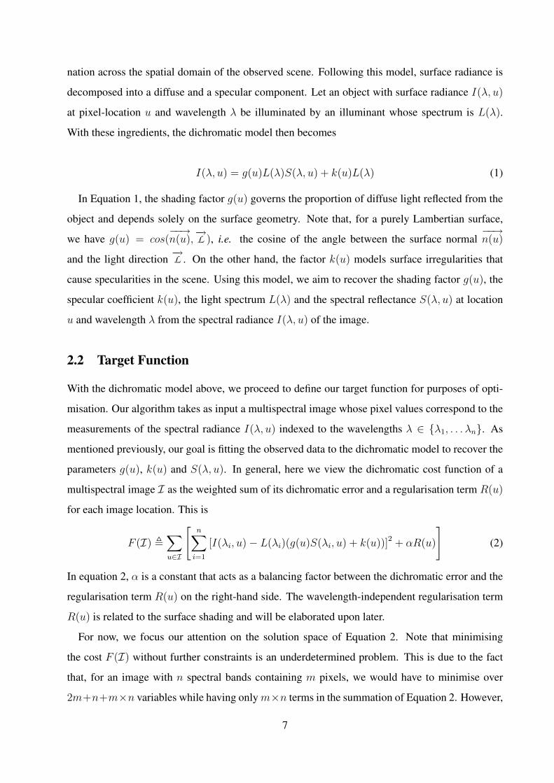
nation across the spatial domain of the observed scene. Following this model, surface radiance is

decomposed into a diffuse and a specular component. Let an object with surface radiance I(λ, u)

at pixel-location u and wavelength λ be illuminated by an illuminant whose spectrum is L(λ).

With these ingredients, the dichromatic model then becomes

I(λ, u) = g(u)L(λ)S(λ, u) + k(u)L(λ) (1)

In Equation 1, the shading factor g(u) governs the proportion of diffuse light reflected from the

object and depends solely on the surface geometry. Note that, for a purely Lambertian surface,

we have g(u) = cos(−−→n(u),

−→L ), i.e. the cosine of the angle between the surface normal

−−→n(u)

and the light direction−→L . On the other hand, the factor k(u) models surface irregularities that

cause specularities in the scene. Using this model, we aim to recover the shading factor g(u), the

specular coefficient k(u), the light spectrum L(λ) and the spectral reflectance S(λ, u) at location

u and wavelength λ from the spectral radiance I(λ, u) of the image.

2.2 Target Function

With the dichromatic model above, we proceed to define our target function for purposes of opti-

misation. Our algorithm takes as input a multispectral image whose pixel values correspond to the

measurements of the spectral radiance I(λ, u) indexed to the wavelengths λ ∈ λ1, . . . λn. As

mentioned previously, our goal is fitting the observed data to the dichromatic model to recover the

parameters g(u), k(u) and S(λ, u). In general, here we view the dichromatic cost function of a

multispectral image I as the weighted sum of its dichromatic error and a regularisation term R(u)

for each image location. This is

F (I) ,∑u∈I

[n∑

i=1

[I(λi, u)− L(λi)(g(u)S(λi, u) + k(u))]2 + αR(u)

](2)

In equation 2, α is a constant that acts as a balancing factor between the dichromatic error and the

regularisation term R(u) on the right-hand side. The wavelength-independent regularisation term

R(u) is related to the surface shading and will be elaborated upon later.

For now, we focus our attention on the solution space of Equation 2. Note that minimising

the cost F (I) without further constraints is an underdetermined problem. This is due to the fact

that, for an image with n spectral bands containing m pixels, we would have to minimise over

2m+n+m×n variables while having only m×n terms in the summation of Equation 2. However,

7

we notice that this problem can be further constrained if the model is applied to smooth surfaces

made of the same material, i.e. the albedo is uniform across the patch or image region under

consideration. This imposes two constraints. Firstly, all locations on the surface share a common

diffuse reflectance. Therefore, a uniform albedo surface P is assumed to have the same reflectance

for each pixel u ∈ P , S(λi, u) = SP (λi). Note that this constraint significantly reduces the number

of unknowns S(λi, u) from m×n to N×n, where N is the number of surface albedos in the scene.

In addition, the smooth variation of the patch geometry allows us to formulate the regularisation

term R(u) in equation 2 as a function of the shading factor g(u). In brief, smooth, uniform albedo

surface patches naturally provide constraints so as to reduce the number of unknowns significantly

while providing a plausible formulation of the regularisation term R(u).

Following the rationale above, we proceed to impose constraints on the minimisation problem at

hand. For a smooth, uniform-albedo surface patch P ∈ I, we consider the following cost function

F (P ) ,∑u∈P

[n∑

i=1

[I(λi, u)− L(λi)(g(u)SP (λi) + k(u))]2 + αR(u)

]

As before, we have S(λi, u) = SP (λi), for all u ∈ P . Furthermore, the smoothness constraint

on the patch implies that the shading factor g(u) should vary smoothly across the pixels in P .

This constraint can be effectively formulated by minimising the variation of gradient magnitude

of the shading map. This, effectively, precludes discontinuities in the shading map of P via the

regularisation term

R(u) ,[∂g(u)

∂x(u)

]2

+

[∂g(u)

∂y(u)

]2

(3)

where the variables x(u) and y(u) are the column and row coordinates, respectively, for pixel

location u.

Thus, by making use of the set P of uniform-albedo patches in the image I, we can recover the

dichromatic model parameters by minimising the target function

F ∗(I) ,∑P∈P

F (P )

=∑P∈P

∑u∈P

[n∑

i=1

[I(λi, u)− L(λi)(g(u)SP (λi) + k(u))]2 + αR(u)

](4)

as an alternative to F (I).

8

2.3 Light Spectrum Recovery

2.3.1 Homogeneous Patch Selection

In the previous section, we formulated the recovery of the dichromatic model parameters as an

optimisation procedure over the surface patch-set P . In this section, we describe our method for

automatically selecting uniform-albedo surface patches for the minimisation of the cost function

in Equation 4. The automatic patch selection method presented here allows the application of our

method to arbitrary images. It is worth noting that this contrasts with other methods elsewhere in

the literature [21, 22, 55, 56], which are only applicable to pre-segmented images.

Our patch selection strategy is performed as follows. We first subdivide the image into patches

of equal size in a lattice-like fashion. For each patch, we fit a two-dimensional hyperplane to the

radiance vectors of the pixels in the patch. Next, we note that, in perfectly dichromatic patches,

the wavelength-indexed radiance vector of each pixel lies perfectly in this hyperplane, i.e. the

dichromatic plane. To allow for noise effect, we regard dichromatic patches as those containing a

percentage of at most tp pixels whose radiance vectors deviate from their projection given by the

Singular Value Decomposition (SVD) in [55]. We do this by setting a threshold ta on the angular

deviation from the dichromatic plane, where tp and ta are global parameters.

However, not all these patches are useful for purposes of illumination spectrum recovery. This

is due to the fact that perfectly diffuse surfaces do not provide any information regarding the illu-

minant spectrum. The reason being that, a spectral radiance vector space for this kind of surfaces

is one-dimensional, spanned only by the wavelength-indexed diffuse radiance vector. On the other

hand, the dichromatic model implies that the specularities have the same spectrum as the illumi-

nant, where the specular coefficient can be viewed as a scaling factor solely dependent on the

surface shading.

Thus, for the recovery of the dichromatic model parameters, we only use highly specular patches

by selecting regions with the highest contrast amongst those deemed to have a uniform albedo. We

recover the contrast of each patch by computing the variance of the mean radiance over the spectral

domain. These highly specular patches provide a means to the recovery of the light spectrum. This

is due to the fact that, for highly specular surface patches with uniform albedo, the surface diffuse

radiance vector and the illuminant vector span a hyperplane in the radiance vector space. This

is a well known property in colour constancy, where a number of approaches [24, 33, 37] have

employed subspace projection for purposes of light power spectrum recovery.

9

I(u): the spectral radiance vector at image pixel u, I(u) = [I(λ1, u), . . . I(λn, u)]T

L : the spectral power vector of the illuminant, L = [L(λ1), . . . L(λn)]T

SP : the common spectral reflectance vector for each patch P , SP = [SP (λ1), . . . SP (λn)]T

gP : the shading map of all pixels in patch P , gP = [g(u1), . . . g(ul)]T

with u1, . . . ul being all the pixels in the patch P

g : the shading map of all the patches, g = [gTP1

, . . . gTPr

]T

where P1, . . . Pr are all patches in PkP : the specularity map of all pixels in patch P , kP = [k(u1), . . . k(ul)]

T

k : the specularity map of all the patches, k = [kTP1

, . . . kTPr

]T

Figure 1: Notation for Section 2.3.2.

2.3.2 Optimisation Procedure

Making use of the notation in Figure 1, we now present the optimisation procedure employed in

our method. Here, we adopt an iterative approach so as to find the variables L, SP , gP and kP

which yield the minimum of the cost function in Equation 4. At each iteration, we minimise the

cost function with respect to L and the triplet gP , kP , SP in separate steps.

The procedure presented here is, in fact, a coordinate descent approach [6] which aims at min-

imising the cost function. The step sequence of our minimisation strategy is summarised in the

pseudocode of Algorithm 1. The coordinate descent approach comprises two interleaved min-

imisation steps. At each iteration, we index the dichromatic variables to iteration number t and

optimise the objective function, in interleaved steps, with respect to the two subsets of variables

gP , kP , SP, L. Once the former variables are at hand, we can obtain optimal values for the

latter ones. We iterate between these two steps until convergence is reached.

The algorithm commences by initialising the unknown light spectrum L(λ) to an unbiased uni-

form illumination spectrum, as indicated in Line 1 of Algorithm 1. It terminates once the illumi-

nant spectrum does not change, in terms of angle, by an amount beyond a preset global threshold

tL between two successive iterations. In the following two subsections we show that the two opti-

misation steps above can be employed to obtain the optimal values of the dichromatic parameters

in closed form.

10

Algorithm 1 Estimate dichromatic variables from a set of homogeneous patchesRequire: Image I with radiance I(λ, u) for each band λ ∈ λ1, . . . λn and location u

and the collection of homogeneous patches PEnsure: L, SP , g, k, where

L: the estimated illuminant spectrum.

SP : the diffuse reflectance of each surface patch P .

g, k: the diffuse and specular reflection coefficients at all locations.

1: t ← 1; L0 ← 1T

2: while true do

3: for all P ∈ I do

4: [gtP , kt

P , StP ] ← argmingP ,kP ,SP

F (P )|Lt−1

5: end for

6: [Lt] ← argminL,SP1,...,SPr

∑P∈P F (P )|gt,kt

7: if ∠(Lt, Lt−1) < tL then

8: break

9: else

10: t ← t + 1

11: end if

12: end while

13: return Lt, gt, kt, StP1

, . . . , StPr

Recovery of the Patch-set Surface ShadingIn the first step, we estimate the optimal surface reflectance and shading given the light spectrum

Lt−1 recovered at iteration t − 1. This corresponds to Lines 3–5 in Algorithm 1. Note that, at

iteration t, we can solve for the unknowns gtP , kt

P and StP separately for each surface patch P . This

is because, for each patch, these variables appear in a separate term in Equation 4. This step is,

therefore, reduced to minimising

F (P )|Lt−1 =∑u∈P

[‖I(u)− g(u)Dt−1P − k(u)Lt−1‖2 + αR(u)

](5)

where the diffuse radiance vector Dt−1P , Lt−1 • SP is the component-wise multiplication of the

illuminant and surface reflectance spectra, and ‖.‖ denotes the L2-norm of the argument vectors.

Note that the minimisation above involves 2|P | + n unknowns, where |P | is the number of

11

pixels in patch P . Hence, it becomes computationally intractable when the surface area is large.

In practice, the selected patches need only be large enough so as to gather useful statistics from

the radiance information. Moreover, as mentioned earlier, we can further reduce the degrees of

freedom of the unknowns by noting that the spectral radiance vectors at all pixels in the same

surface lie in a 2-dimensional subspace Q ⊂ Rn, spanned by the diffuse radiance vector Dt−1P and

the light vector Lt−1. This is a characteristic of the dichromatic model that has been widely utilised

by prior work on colour constancy [21, 22, 55, 56].

Having all the pixel radiance vectors I(u) at hand, one can obtain the subspace Q via Singular

Value Decomposition (SVD). Denote the two basis vectors resulting from this SVD operation

z1 and z2 and, accordingly, let the subspace be Q = span(z1, z2). Since Dt−1P ∈ Q, we can

parameterise Dt−1P up to scale as Dt−1

P = vz1 + z2.

Likewise, the light vector Lt−1 ∈ Q can also be decomposed as Lt−1 = w1z1 + w2z2, where

the values of w1 and w2 are two known scalars. Furthermore, the dichromatic plane hypothesis

also implies that, given the light vector Lt−1 and the surface diffuse radiance vector Dt−1P , one can

decompose any pixel radiance I(u) into a linear combination of the former two vectors. In other

words,

I(u) = g(u)Dt−1P + k(u)Lt−1

= (g(u)v + k(u)w1)z1 + (g(u) + k(u)w2)z2 (6)

Having obtained the basis vectors z1, z2, we can compute the mapping of the pixel radiance I(u)

onto the subspace Q. This is done with respect to this basis by means of projection so as to obtain

the scalars τ1(u), τ2(u) such that

I(u) = τ1(u)z1 + τ2(u)z2 (7)

Further, by equating the right hand sides of Equations 6 and 7, we obtain

g(u) =w2τ1(u)− w1τ2(u)

w2v − w1

(8)

k(u) =τ2(u)v − τ1(u)

w2v − w1

(9)

From Equations 8 and 9, we note that g(u) and k(u) are univariate rational functions of v.

Moreover, Dt−1P is a linear function with respect to v. We also observe that the term R(u) is only

dependent on g(u). Therefore, the objective function in Equation 5 can be reduced to a univariate

12

rational function of v. Thus, substituting the Equations 8 and 9 into the first and second term on

the right hand side of Equation 5, we have

F (P )|Lt−1 =∑u∈P

‖I(u)− w2τ1(u)− w1τ2(u)

w2v − w1

(vz1 + z2)− τ2(u)v − τ1(u)

w2v − w1

Lt−1‖2

+∑u∈P

α

(w2v − w1)2

[(∂m(u)

∂x(u)

)2

+

(∂m(u)

∂y(u)

)2]

=∑u∈P

1

(w2v − w1)2‖ (

I(u)w2 − (w2τ1(u)− w1τ2(u))z1 − τ2(u)Lt−1)v

− (I(u)w1 − (w2τ1(u)− w1τ2(u))z2 − τ1(u)Lt−1

) ‖2

+α

(w2v − w1)2

∑u∈P

[(∂m(u)

∂x(u)

)2

+

(∂m(u)

∂y(u)

)2]

=∑u∈P

‖p(u)v − q(u)

w2v − w1

‖2 +αN

(w2v − w1)2

=∑u∈P

‖p(u)

w2

+w1

w2p(u)− q(u)

w2v − w1

‖2 +αN

(w2v − w1)2

=∑u∈P

‖p(u)‖2

w22

+2

w2v − w1

∑u∈P

〈p(u)

w2

,w1

w2

p(u)− q(u)〉

+1

(w2v − w1)2

(∑u∈P

‖w1

w2

p(u)− q(u)‖2 + αN

)(10)

where 〈., .〉 denotes the inner-product of two vectors, and

m(u) = w2τ1(u)− w1τ2(u)

p(u) = I(u)w2 − (w2τ1(u)− w1τ2(u))z1 − τ2(u)Lt−1

q(u) = I(u)w1 − (w2τ1(u)− w1τ2(u))z2 − τ1(u)Lt−1

N =∑u∈P

[(∂m(u)

∂x(u)

)2

+

(∂m(u)

∂y(u)

)2]

Note that p(u), q(u), w1 and w2 are known given the vector Lt−1. With the change of variable

r = 1w2v−w1

we can write the right hand side of Equation 10 as a quadratic function of r whose

minimum is attained at

r∗ = −∑

u∈P 〈p(u)w2

, w1

w2p(u)− q(u)〉∑

u∈P ‖w1

w2p(u)− q(u)‖2 + αN

(11)

This gives the corresponding minimiser v∗ = 1w2

( 1r∗ + w1). Hence, given the illuminant spec-

trum Lt−1, one can recover gP , kP by substituting the optimal value of v into Equations 8 and 9.

The diffuse radiance component is computed as DtP = v∗z1 + z2, and the spectral reflectance at

wavelength λ is given by StP (λ) =

DtP (λ)

Lt−1(λ).

13

Recovery of the Illuminant SpectrumIn the second step of each iteration t, we solve for Lt and St

P1, . . . , St

Prgiven gt

P and ktP . Since

the second term R(u) in Equation 4 is wavelength-independent, the optimisation problem in line 6

of Algorithm 1 can be reduced to minimising

F ∗(I)|gt,kt =∑P∈P

∑u∈P

‖I(u)− gt(u)DP − kt(u)L‖2

=∑P∈P

∑u∈P

n∑i=1

(I(λi, u)− gt(u)DP (λi)− kt(u)L(λi)

)2 (12)

where DP = L • SP

Since the objective function 12 is quadratic, and, therefore convex with respect to L and DP , the

optimal values of these variables can be obtained by equating the respective partial derivatives of

F ∗(I)|gt,kt to zero. These partial derivatives are given by

∂F ∗(I)|gt,kt

∂L(λi)= −2

∑P∈P

∑u∈P


)kt(u)

∂F ∗(I)|gt,kt

∂DP (λi)= −2

∑u∈P


)gt(u)

Equating the above equations to zero, we obtain

L(λi) =

∑P∈P

∑u∈P [kt(u)I(λi, u)− gt(u)kt(u)DP (λi)]∑

P∈P∑

u∈P (kt(u))2(13)

DP (λi) =

∑u∈P [gt(u)I(λi, u)− gt(u)kt(u)L(λi)]∑

u∈P (gt(u))2(14)

From Equations 13 and 14, the illuminant spectrum can be solved in closed form as

L∗(λi) =

∑P∈P

∑u∈P kt(u)I(λi, u)−∑

P∈P

[(∑

u∈P gt(u)kt(u))(∑

u∈P gt(u)I(λi,u))∑u∈P (gt(u))2

]

∑P∈P

∑u∈P (kt(u))2 −∑

P∈P

[(∑

u∈P gt(u)kt(u))2

∑u∈P (gt(u))2

] (15)

2.4 Shading, Reflectance and Specularity Recovery

Note that, in the optimisation scheme above, we recover the reflectance, shading and specularity

factors for pixels in each patch P ∈ P used for the recovery of the illuminant spectrum. This

implies that, although we have only computed the variables g(u), k(u) and S(., u) for pixel-sites

u ∈ P , we have been able to recover the illuminant spectrum L. Since L is a global photometric

variable in the scene, we can recover the remaining dichromatic variables making use of L in a

14

straightforward manner. These include shading, reflectance and specularity factors for all image

pixels.

For this purpose, we assume the input scene is composed of smooth surfaces with slowly vary-

ing reflectance. In other words, the neighbourhood of each pixel can be regarded as a locally

smooth patch made of the same material, i.e. all the pixels in the neighbourhood share the same

spectral reflectance. Given the illuminant spectrum, we can obtain the shading, specularity and

reflectance of the neighbourhood at the pixel of interest by applying the procedure corresponding

to line 4 in Algorithm 1. This corresponds to the application of the first of the two steps used in

the optimisation method presented in the section above.

The pseudocode of this algorithm is summarised in Algorithm 2. Note that the assumption

of smooth surfaces with slowly varying reflectance is applicable to a large category of scenes

where surfaces have a low degree of texture, edges and occlusion. Following this assumption,

the reflectance at each pixel is recovered as the shared reflectance of its surrounding patch. To

estimate the shading and specularity, one can apply the closed-form formulae of these, as shown

in Equations 8 and 9. These formulae yield exact solutions in the ideal condition, which requires

that all the pixel radiance vectors lie in the same dichromatic hyperplane spanned by the illuminant

spectrum and the diffuse radiance vector.

However, in practice, it is common for multi-spectral images to contain noise which breaks

down this assumption and renders the above quotient expressions numerically unstable. Therefore,

to enforce a smooth variation of the shading factor across pixels, we recompute the shading and

specularity coefficients after obtaining the spectral reflectance. This is due to the observation that

the reflectance spectrum is often more stable than the other two variables, i.e. shading and specu-

larity factors. Specifically, one can compute the shading and specular coefficients as those resulting

from the projection of pixel radiance onto the subspace spanned by the illuminant spectrum and

the diffuse radiance spectrum vectors.

15

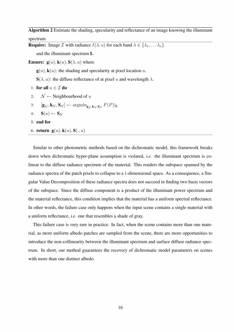
Algorithm 2 Estimate the shading, specularity and reflectance of an image knowing the illuminant

spectrumRequire: Image I with radiance I(λ, u) for each band λ ∈ λ1, . . . λn

and the illuminant spectrum L

Ensure: g(u), k(u), S(λ, u) where

g(u), k(u): the shading and specularity at pixel location u.

S(λ, u): the diffuse reflectance of at pixel u and wavelength λ.

1: for all u ∈ I do

2: N ← Neighbourhood of u

3: [gN , kN , SN ] ← argmingN ,kN ,SN F (P )|L4: S(u) ← SN

5: end for

6: return g(u), k(u), S(., u)

Similar to other photometric methods based on the dichromatic model, this framework breaks

down when dichromatic hyper-plane assumption is violated, i.e. the illuminant spectrum is co-

linear to the diffuse radiance spectrum of the material. This renders the subspace spanned by the

radiance spectra of the patch pixels to collapse to a 1-dimensional space. As a consequence, a Sin-

gular Value Decomposition of these radiance spectra does not succeed in finding two basis vectors

of the subspace. Since the diffuse component is a product of the illuminant power spectrum and

the material reflectance, this condition implies that the material has a uniform spectral reflectance.

In other words, the failure case only happens when the input scene contains a single material with

a uniform reflectance, i.e. one that resembles a shade of gray.

This failure case is very rare in practice. In fact, when the scene contains more than one mate-

rial, as more uniform albedo patches are sampled from the scene, there are more opportunities to

introduce the non-collinearity between the illuminant spectrum and surface diffuse radiance spec-

trum. In short, our method guarantees the recovery of dichromatic model parameters on scenes

with more than one distinct albedo.

16

3 Imposing Smoothness Constraints

In Section 2.2, we addressed the need of enforcing the smoothness constraint on the shading field

g = g(u)u∈I using the regularisation term R(u) in Equation 2. In Equation 3, we present a reg-

ulariser that encourages the slow spatial variation of the shading field. There are two reasons for

using this regulariser in the optimisation framework introduced in the previous sections. Firstly,

it yields a closed-form solution for the surface shading and reflectance, given the illuminant spec-

trum. Secondly, it is reminiscent of smoothness constraints imposed upon shape from shading

approaches and, hence, it provides a link between other methods in the literature, such as that in

[59] and the optimisation method in the previous sections. However, we need to emphasise that

the optimisation procedure above by no means implies that the framework is not applicable to al-

ternative regularisers. In fact, our target function is flexible in the sense that other regularisation

functions can be formulated dependent on the surface at hand.

In this section, we introduce a number of alternative regularisers on the shading field that are ro-

bust to noise and outliers and adaptive to the surface shading variation. To this end, we commence

by introducing robust regularisers. We then present extensions based upon the surface curvature

and the shape index.

To quantify the smoothness of shading, an option is to treat the gradient of the shading field as the

smoothness error. In Equation 3, we have introduced a quadratic error function of the smoothness.

However, in certain circumstances, enforcing the quadratic regulariser as introduced in Equation 2

causes the undesired effect of oversmoothing the surface. This well-known phenomenon has been

experienced in a number of developments [11, 31] in the field of Shape from Shading. It is worth

noting in passing that ample work exists in the literature addressing the over-smoothing tendency

of quadratic regularisers used for enforcing smoothness constraints on gradients [17, 59, 60].

As an alternative, we utilise kernel functions stemming from the field of robust statistics. For-

mally speaking, a robust kernel function ρσ(η) quantifies an energy associated with both the resid-

ual η and its influence function, i.e. measures sensitivity to changes in the shading field. Each

residual is, in turn, assigned a weight as defined by an influence function Γσ(η). Thus the en-

ergy is related to the first-moment of the influence function as ∂ρσ(η)∂η

= ηΓσ(η). Table 1 shows

the formulae for Tukey’s bi-weight [26], Li’s Adaptive Potential Functions [38] and Huber’s M-

estimators [30].

17

Estimator Robust kernel ρσ(η) Influence function Γσ(η)

Tukey ρσ(η) =

σ(1− (

1− ( ησ)2

)3)

if |η| < σ

σ otherwiseΓσ(η) =

(1− ( η

σ)2

)2 if |η| < σ

0 otherwise

Li ρσ(η) = σ(1− exp

(−η2

σ

))Γσ(η) = exp

(−η2

σ

)

Huber ρσ(η) =

η2 if |η| < σ

2σ|η| − σ2 otherwiseΓσ(x) =

1 if |η| < σ

σ|η| otherwise

Table 1: Robust kernels and influence functions.

3.1 Robust Shading Smoothness Constraint

Having introduced the above robust estimators, we proceed to employ them as regularisers for the

target function. Here, several possibilities exist. One of them is to directly minimise the shading

variation by defining robust regularisers with respect to the shading gradient. In this case, the

regulariser R(u) is given by the following formula

R(u) = ρσ

(∣∣∣∣∂g

∂x

∣∣∣∣)

+ ρσ

(∣∣∣∣∂g

∂y

∣∣∣∣)

(16)

Despite effective, the formula above still employs the gradient of the shading field as a measure

of smoothness. In the next section, we explore the use of curvature as a measure of consistency.

3.2 Curvature Consistency

Alternatively, one can instead consider the intrinsic characteristics of the surface at hand given by

its curvature. Specifically, Ferrie and Lagarde [17] have used the global consistency of principal

curvatures to refine surface estimates in Shape from Shading. Moreover, ensuring the consistency

of curvature directions does not necessarily imply a large penalty for discontinuities of orientation

and depth. Therefore, this measure can avoid oversmoothing, which is a drawback of the quadratic

smoothness error.

The curvature consistency can be defined on the shading field by treating it as a manifold. To

commence, we define the structure of the shading field using its Hessian matrix

H =

∂2g∂x2

∂2g∂x∂y

∂2g∂y∂x

∂2g∂y2

The principal curvatures of the manifold are hence defined as the eigenvalues of the Hessian

matrix. Let these eigenvalues be denoted by κ1 and κ2, where κ1 ≥ κ2. Moreover, we can use the

18

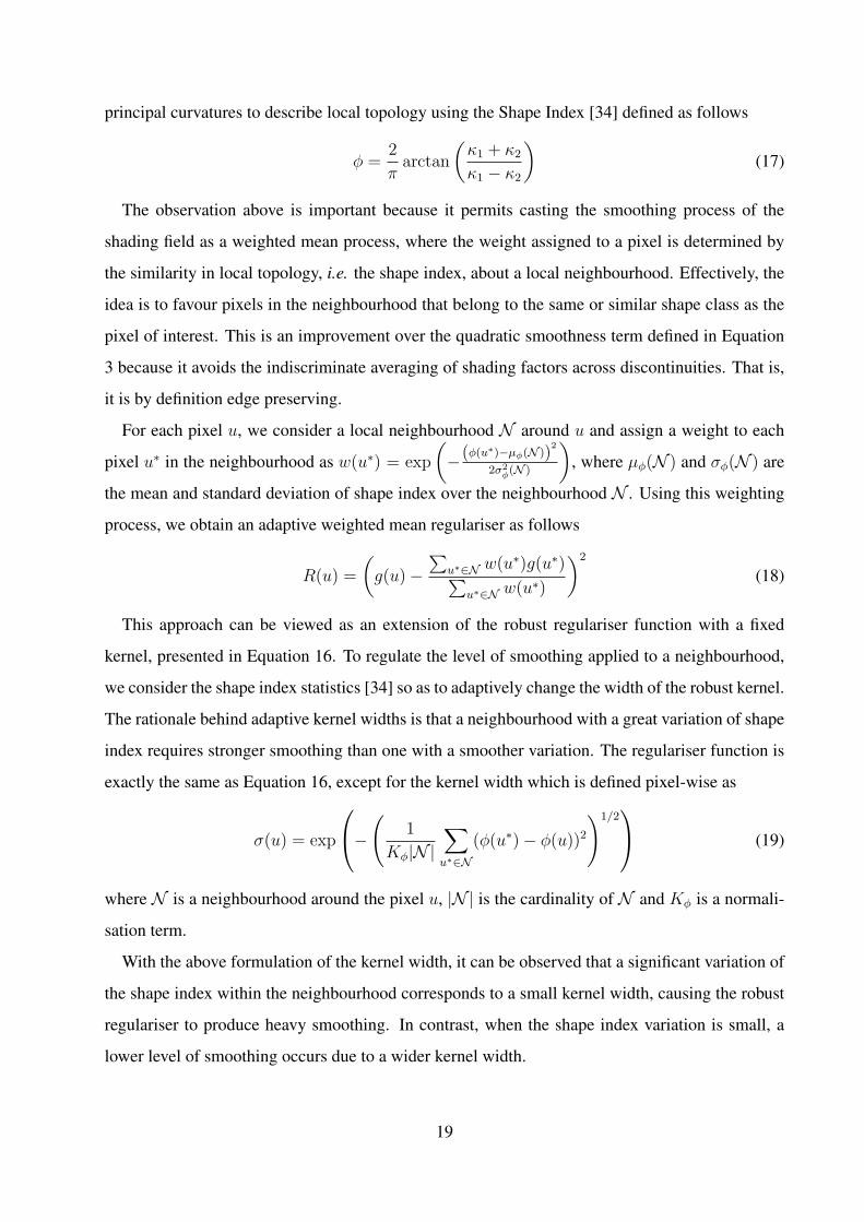
principal curvatures to describe local topology using the Shape Index [34] defined as follows

φ =2

πarctan

(κ1 + κ2

κ1 − κ2

)(17)

The observation above is important because it permits casting the smoothing process of the

shading field as a weighted mean process, where the weight assigned to a pixel is determined by

the similarity in local topology, i.e. the shape index, about a local neighbourhood. Effectively, the

idea is to favour pixels in the neighbourhood that belong to the same or similar shape class as the

pixel of interest. This is an improvement over the quadratic smoothness term defined in Equation

3 because it avoids the indiscriminate averaging of shading factors across discontinuities. That is,

it is by definition edge preserving.

For each pixel u, we consider a local neighbourhood N around u and assign a weight to each

pixel u∗ in the neighbourhood as w(u∗) = exp

(−(φ(u∗)−µφ(N ))

2

2σ2φ(N )

), where µφ(N ) and σφ(N ) are

the mean and standard deviation of shape index over the neighbourhood N . Using this weighting

process, we obtain an adaptive weighted mean regulariser as follows

R(u) =

(g(u)−

∑u∗∈N w(u∗)g(u∗)∑

u∗∈N w(u∗)

)2

(18)

This approach can be viewed as an extension of the robust regulariser function with a fixed

kernel, presented in Equation 16. To regulate the level of smoothing applied to a neighbourhood,

we consider the shape index statistics [34] so as to adaptively change the width of the robust kernel.

The rationale behind adaptive kernel widths is that a neighbourhood with a great variation of shape

index requires stronger smoothing than one with a smoother variation. The regulariser function is

exactly the same as Equation 16, except for the kernel width which is defined pixel-wise as

σ(u) = exp

−

(1

Kφ|N |∑

u∗∈N(φ(u∗)− φ(u))2

)1/2 (19)

where N is a neighbourhood around the pixel u, |N | is the cardinality of N and Kφ is a normali-

sation term.

With the above formulation of the kernel width, it can be observed that a significant variation of

the shape index within the neighbourhood corresponds to a small kernel width, causing the robust

regulariser to produce heavy smoothing. In contrast, when the shape index variation is small, a

lower level of smoothing occurs due to a wider kernel width.

19

Note that the use of the robust regularisers introduced earlier in this section as an alternative

to the quadratic regulariser does not preclude the applicability of the optimisation framework de-

scribed in Section 2.3.2. In fact, the change of regulariser only affects the formulation of the target

function in Equation 10, in which the shading factor g(u) can be expressed as a univariate func-

tion as given in Equation 8. Since all the above robust regularisers are only dependent on the

shading factor, the resulting target function is still a function of the variable r , 1w2v−w1

. Fur-

ther, by linearisation of the robust regularisers, one can still numerically express the regulariser

as a quadratic function of the variable r. Subsequently, the closed-form solution presented earlier

stands as originally described.

4 Adaptation to Trichromatic Imagery

In this section, we show how to utilise the optimisation method above to recover the dichromatic

parameters from trichromatic images. To this end, we transform the dichromatic model for mul-

tispectral images into one for trichromatic imagery. Let us denote the spectral sensitivity func-

tion of the trichromatic sensor c (where c ∈ R, G, B) by Cc(λ). The response of the sensor

c to the spectral irradiance arriving at the location u is given by Ic(u) =∫

ΩE(λ, u)Cc(λ)dλ,

where E(λ, u) is the image irradiance and Ω is the spectrum of the incoming light. Further-

more, it is well-known that the image irradiance is proportional to the scene radiance I(λ, u),

i.e. E(λ, u) = Kopt cos4 β(u)I(λ, u), where β(u) is the angle of incidence of the incoming light

ray on the lens and Kopt is a constant only dependent on the optics of the lens [28]. Hence, we

have

Ic(u) = Kopt cos4 β(u)

∫

Ω

I(λ, u)Cc(λ)dλ

= Kopt cos4 β(u)

∫

Ω

(g(u)L(λ)S(λ, u) + k(u)L(λ))Cc(λ)dλ

= Kopt cos4 β(u)

∫

Ω

L(λ)S(λ, u)Cc(λ)dλ + Kopt cos4 β(u)k(u)

∫

Ω

L(λ)Cc(λ)dλ

= g∗(u)Dc(u) + k∗(u)Lc

where g∗(u) = Kopt cos4 β(u)g(u) and k∗(u) = Kopt cos4 β(u)k(u).

Here we notice that Dc(u) =∫

ΩL(λ)S(λ, u)Cc(λ)dλ and Lc(u) =

∫Ω

L(λ)Ci(λ)dλ are the

c component of the surface diffuse colour corresponding to the location u and of the illuminant

colour, respectively.

20

The dichromatic cost function for the trichromatic image I of a scene is formulated as

F (I) ,∑u∈I

∑

c∈R,G,B[Ic(u)− (g∗(u)Dc(u) + k∗(u)Lc)]

2 + αR(u)

(20)

where R(u) is a spatially varying regularisation term, as described in Equation 2.

It is worth noticing that the cost function in Equation 20 is a special case of Equation 2, where

n = 3. Hence, the method of recovering the dichromatic parameters, as elaborated upon in Sections

2.3.1 and 2.3.2 can be applied to this case in order to recover the trichromatic diffuse colour

D(u) = [DR(u), DG(u), DB(u)]T and illuminant colour L = [LR, LG, LB]T , as well as the shading

and specular factors g(u) and k(u) up to a multiplier.

5 Experiments

In this section, we perform experiments on a number of image databases so as to verify the accuracy

of the recovered dichromatic parameters. Our datasets include indoor and outdoor multispectral

and RGB images with uniform and cluttered backgrounds, under natural and artificial lighting

conditions. For this purpose, we have acquired in-house two multi-spectral image databases cap-

tured in the visible and near-infrared ranges. These consist of indoor images taken under artificial

light sources and outdoor images under natural sunlight and skylight. From these two databases,

two trichromatic image databases are synthesized for the spectral sensitivity functions of a Canon

10D and a Nikon D70 camera sensor and the CIE standard RGB colour matching functions [15].

Apart from these databases, we have also compared the performance of our algorithm with the

alternatives on the benchmark dataset reported by Barnard et al. in [3].

The indoor database includes images of 51 human subjects, each captured under one of 10

directional light sources with varying directions and spectral power. The light sources are divided

into two rows. The first of these is placed above the camera system and the second one at the

same height as the cameras. The main direction of the lights is adjusted so as to point towards the

centre of the scene. The imagery has been acquired using a pair of OKSI Turnkey Hyperspectral

Cameras. These cameras are equipped with Liquid Crystal Tunable Filters which allow multi-

spectral images to be resolved up to 10nm in both the visible (430–720nm) and the near infrared

(650–990nm) wavelength ranges. To obtain the ground truth illuminant spectrum for each image,

we have measured the average radiance reflected from a white calibration target, i.e. a LabSphere

21

Spectralon, illuminated by the light sources under consideration. Using the same camera system

and calibration target, we have captured the outdoor images of a paddock from four different

viewpoints, each from seven different viewing angles at different times of the day.

In the following experiments, we explore the utility of the recovered parameters of the dichro-

matic model for multiple applications. Throughout these experiments, our method is shown to be

most successful in delivering competitive performance for illumination spectrum recovery and ma-

terial recognition purposes. Therefore, we present the main bulk of the experiments in Section 5.1,

where we demonstrate the effectiveness of our method for illumination spectrum recovery. In Sec-

tion 5.2, we present results for skin recognition and material clustering tasks. The purpose of the

section is two-fold, one of which is to assess the robustness of the recovered reflectance for mate-

rial recognition, the other is to reaffirm the accuracy of the illumination spectrum recovery results

presented in Section 5.1. Lastly, we explore the use of the recovered shading and specularity coef-

ficients for specularity removal in Section 5.3. Note that, although the method was not originally

designed for specularity removal, it may also be applied for such a purpose with moderate success.

5.1 Illumination Spectrum Recovery

For our experiments on illumination spectra recovery, we compare the results yielded by our

method to those delivered by the colour constancy method proposed by Finlayson and Schaefer

[21]. In [21], illuminant colours are estimated based on the dichromatic model without prior as-

sumptions on the illuminant statistics. Although their experiments were performed on trichromatic

imagery, this method can be adapted to multispectral data in a straightforward manner. Their ap-

proach relies on the dichromatic plane hypothesis. This is, that the dichromatic model implies a

two-dimensional colour space of pixels in patches with homogeneous reflectance. Utilising this

idea, illumination estimation is cast as an optimisation problem so as to maximise the total projec-

tion length of the light colour vector on all the dichromatic planes. Geometrically, this approach

predicts the illuminant colour as the intersection of dichromatic planes, which may lead to a nu-

merically unstable solution when the angle between dichromatic planes are small.

Finlayson and Schaefer’s method can be adapted to multispectral images as follows. First, we

employ our automatic patch selection method to provide homogeneous patches as input for their

colour constancy algorithm. Secondly, we solve the eigen-system of the sum of projection matrices

on the dichromatic planes. The light colour vector is the eigenvector corresponding to the largest

22

eigenvalue.

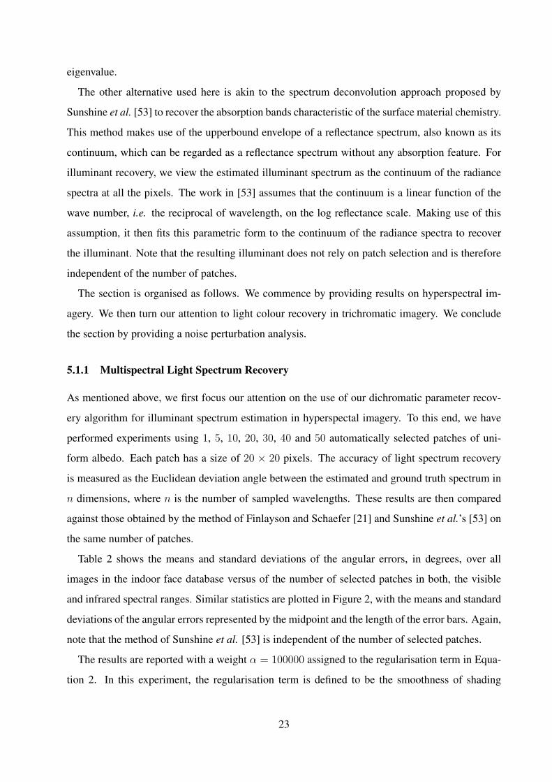
The other alternative used here is akin to the spectrum deconvolution approach proposed by

Sunshine et al. [53] to recover the absorption bands characteristic of the surface material chemistry.

This method makes use of the upperbound envelope of a reflectance spectrum, also known as its

continuum, which can be regarded as a reflectance spectrum without any absorption feature. For

illuminant recovery, we view the estimated illuminant spectrum as the continuum of the radiance

spectra at all the pixels. The work in [53] assumes that the continuum is a linear function of the

wave number, i.e. the reciprocal of wavelength, on the log reflectance scale. Making use of this

assumption, it then fits this parametric form to the continuum of the radiance spectra to recover

the illuminant. Note that the resulting illuminant does not rely on patch selection and is therefore

independent of the number of patches.

The section is organised as follows. We commence by providing results on hyperspectral im-

agery. We then turn our attention to light colour recovery in trichromatic imagery. We conclude

the section by providing a noise perturbation analysis.

5.1.1 Multispectral Light Spectrum Recovery

As mentioned above, we first focus our attention on the use of our dichromatic parameter recov-

ery algorithm for illuminant spectrum estimation in hyperspectal imagery. To this end, we have

performed experiments using 1, 5, 10, 20, 30, 40 and 50 automatically selected patches of uni-

form albedo. Each patch has a size of 20 × 20 pixels. The accuracy of light spectrum recovery

is measured as the Euclidean deviation angle between the estimated and ground truth spectrum in

n dimensions, where n is the number of sampled wavelengths. These results are then compared

against those obtained by the method of Finlayson and Schaefer [21] and Sunshine et al.’s [53] on

the same number of patches.

Table 2 shows the means and standard deviations of the angular errors, in degrees, over all

images in the indoor face database versus of the number of selected patches in both, the visible

and infrared spectral ranges. Similar statistics are plotted in Figure 2, with the means and standard

deviations of the angular errors represented by the midpoint and the length of the error bars. Again,

note that the method of Sunshine et al. [53] is independent of the number of selected patches.

The results are reported with a weight α = 100000 assigned to the regularisation term in Equa-

tion 2. In this experiment, the regularisation term is defined to be the smoothness of shading

23

No. Visible spectrum Near-infrared spectrum

patches Our method F & S Sunshine Our method F & S Sunshine

1 17.25± 6.07 20.55± 10.53 9.52± 1.40 7.41± 5.37 25.50± 8.88 19.9± 2.24

5 5.62± 5.54 7.52± 4.90 6.44± 5.09 7.00± 4.56

10 5.81± 5.63 7.42± 4.19 6.65± 5.05 6.98± 4.04

20 6.21± 5.22 7.37± 3.88 6.87± 4.95 7.03± 3.58

30 6.49± 5.53 7.32± 3.65 7.56± 5.18 7.06± 3.46

40 6.66± 5.86 7.29± 3.54 7.85± 5.07 7.06± 3.39

50 6.82± 5.84 7.26± 3.50 7.90± 5.25 7.09± 3.33

Table 2: Accuracy versus the number of patches used for our illuminant estimation method on the multi-

spectral facial image database captured under both the visible and near-infrared spectra, in degrees, com-

pared to Finlayson and Schaefer’s method (F & S) and Sunshine et al.’s method.

(a) Visible spectrum (b) Near-infrared spectrum

Figure 2: Accuracy versus number of patches used of our illuminant estimation method on the multispectral

facial image database, in degrees, compared to Finlayson and Schaefer’s method (F & S) and Sunshine et

al.’s method. The results for both the visible (left) and near-infrared ranges (right) are shown.

variation, as shown in Equation 3. To obtain an optimal value of α, we perform a procedure simi-

lar to the grid search employed in cross validation. The procedure involves applying our algorithm

on a randomly sampled portion of the database several times for different parameter values and

then selecting the value that yields the highest overall performance.

As shown in Table 2, our algorithm achieves a higher accuracy than the alternative methods when

using no more than 20 homogeneous patches for both spectral ranges. It is noticeable that even with

24

a single patch, our method still significantly outperforms Finlayson and Schaefer’s method [21].

This observation is consistent with the well-known fact that the dichromatic plane method and

its variants require at least two homogeneous surfaces to compute the intersection between the

dichromatic planes. In addition, the angular error of the estimated illuminant decreases as the

number of patches increases from 1 to 5. However, as the number of patches grows beyond 5, the

angular error of our method tends to increase. Although our methods remains more accurate than

Finlayson and Schaefer’s method in the visible range, its accuracy is slightly lower than the latter

with more than 20 patches in the near-infrared range. Nonetheless, our method is able to achieve

a reasonable estimate with a small number of homogeneous patches. Lastly, we can conclude that

Sunshine et al.’s method [53] is, in general, inferior to the other two.

To illustrate the statistics in Table 2, we show, in Figure 3, the plots of the estimated spectra

of a light source illuminating an indoor scene. The plots show spectra in both the visible (left

column) and infra-red (right column) ranges. In each row, from top to bottom, we show the results

yielded by our method and the alternatives using a different number of homogeneous patches for

illuminant estimation. As before, we show the plots for 1, 5, 10, 40 and 50 patches. The ground

truth spectra, the spectra estimated by our method, Finlayson and Schaefer’s [21] and Sunshine et

al.’s method [53] are drawn in red, blue, green and magenta, respectively. Note that the highest

value of each spectra is normalised to unity.

This visual illustration is consistent with a common trend in Table 2, that increasing the number

of patches from 1 to 5 yields a significant improvement of accuracy for illumination estimation.

Noticeably, our method outperforms the alternatives in recovering illumination spectra in the visi-

ble range. Meanwhile, its performance for the near-infrared range is comparable to Finlayson and

Schaefer’s [21] and is better than Sunshine et al.’s method [53]. Moreover, our method is more

robust than the others even when it uses a single homogeneous patch for light estimation.

In Table 3 and Figure 4, we show the accuracy of the recovered spectrum of natural sunlight

illuminating the outdoor scene in our dataset. Here our algorithm is applied with a regularisation

weight α = 10000000. With this setting, our method always outperforms the alternatives in the

visible range. Using 20 or more randomly selected patches is sufficient for our method to improve

performance over Finlayson and Schaefer’s [21] on the near-infrared images. As before, our al-

gorithm significantly outperforms the alternative methods in the case of a single uniform albedo

patch. Figure 4 also illustrates the stability of our method with respect to the increase in the num-

ber of selected patches. It is also noticeable that the accuracy of all the algorithms for the outdoor

25

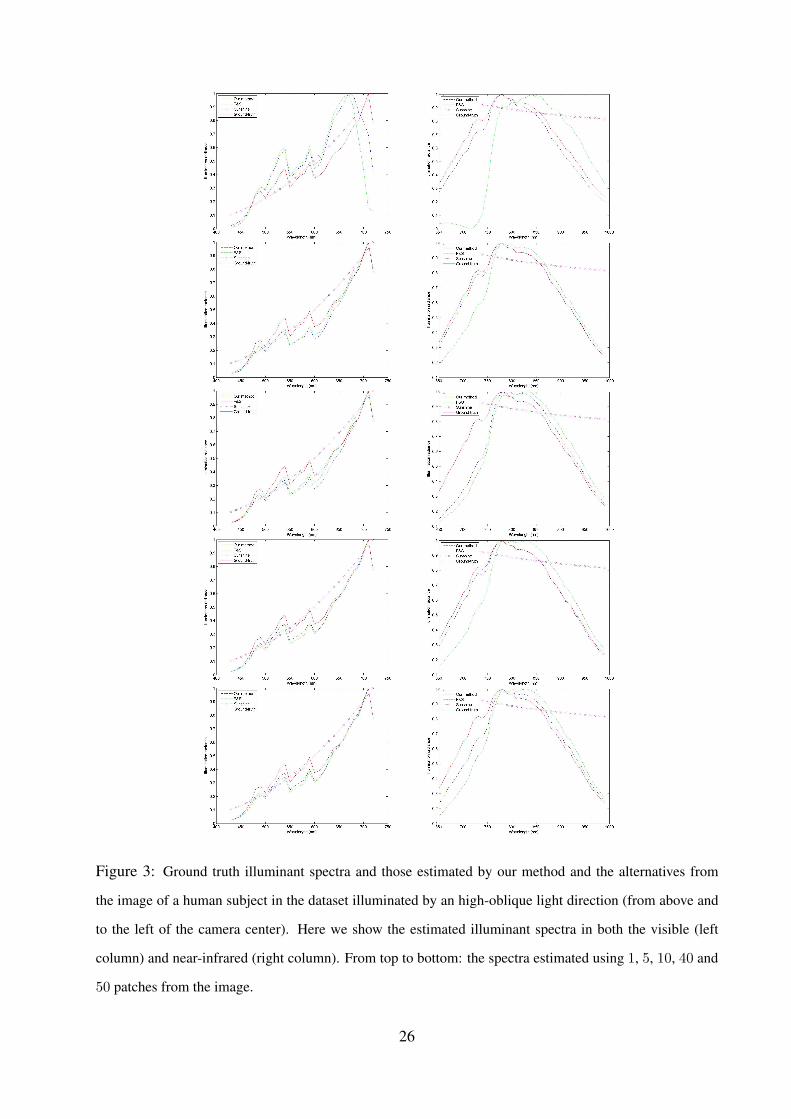
Figure 3: Ground truth illuminant spectra and those estimated by our method and the alternatives from

the image of a human subject in the dataset illuminated by an high-oblique light direction (from above and

to the left of the camera center). Here we show the estimated illuminant spectra in both the visible (left

column) and near-infrared (right column). From top to bottom: the spectra estimated using 1, 5, 10, 40 and

50 patches from the image.

26

No. Visible spectrum Near-infrared spectrum


1 13.93± 2.83 22.17± 5.84 17.91± 5.43 9.35± 4.63 29.46± 8.18 17.13± 2.18

5 13.89± 1.25 14.06± 1.47 8.08± 3.38 6.97± 2.59

10 13.80± 1.17 14.09± 1.35 8.47± 2.58 7.31± 1.80

20 14.00± 1.43 14.03± 1.33 7.07± 2.51 7.20± 1.38

30 13.69± 1.53 14.00± 1.23 6.98± 2.41 7.48± 1.50

40 13.44± 2.09 13.99± 1.22 7.22± 2.48 7.69± 1.59

50 13.85± 1.48 13.97± 1.24 7.33± 2.48 7.74± 1.45

Table 3: Accuracy, in degrees, versus the number of patches used for our illuminant estimation method on

the multispectral outdoor image database captured under both the visible and near-infrared spectra compared

to Finlayson and Schaefer’s method (F & S) and Sunshine et al.’s approach.

(a) Visible spectrum (b) Near-infrared spectrum

Figure 4: Accuracy versus the number of patches used for our illuminant estimation method on the mul-

tispectral outdoor image database, in degrees, compared to Finlayson and Schaefer’s method (F & S) and

Sunshine et al.’s method. The results for both the visible (left) and near-infrared ranges (right) are shown.

27

Figure 5: Ground truth illuminant spectra and those estimated by our method and the alternatives from the

image of an outdoor scene. Here we show the estimated illuminant spectra in both the visible (left column)

and the near-infrared (right column) ranges. From top to bottom: the spectra estimated using 1, 10, 20, 30

and 40 patches from the image.

28

image database is lower than that for the face database due to a wider variation of spectral radiance

across the scene. These trends are visually demonstrated using a number of sample plots of the

estimated spectra of natural sunlight, as shown in Figure 5.

5.1.2 Trichromatic Light Recovery

Next, we turn our attention to the utility of our parameter recovery method for the purpose of

illuminant colour estimation from trichromatic images. To this end, we generate RGB imagery

from the multispectral face and outdoor databases mentioned previously. These are synthesized by

simulating a number of trichromatic spectral responses, including the CIE-1932 colour matching

functions [15] and the camera sensors for a Nikon D70 and a Canon 10D. Furthermore, we apply

our method and the alternatives to the Mondrian and specular image datasets as described by

Barnard et al [4]. We also compare the performance of our algorithm with several colour constancy

approaches described in [3] by the same authors.

To illustrate the effect of varying the value of α, we perform experiments with α = 10000

and α = 100. In Table 4 and Figure 6 we show results for the light estimation accuracy on the

RGB face images with α = 10000 and a patch size of 20 × 20 pixels. Our method outperforms

the alternatives in terms of estimation accuracy and stability when the number of patches (or the

number of available intrinsic colours in the scene) is 5 or less. Another general trend is that our

method and Finlayson and Schaefer’s [21] one improve their accuracy as the number of selected

patches increases. However, this improvement is marginal for our method when we use 20 or more

patches. Meanwhile, the method of Finlayson and Schaefer [21] tends to achieve a closer estimate

to the groundtruth when it is applied on a sufficiently large number of patches from the images

synthesized for the Canon 10D and Nikon D70 sensors. Interestingly, for images simulated for

the colour matching functions, which emulate the human visual perception, our method achieves a

similar accuracy to Finlayson and Schaefer’s [21] across all the number of selected patches, while

being more stable (with lower variance of angular error). In all our experiments, the approach of

Sunshine et. al [53] is the one that delivers the worst performance.

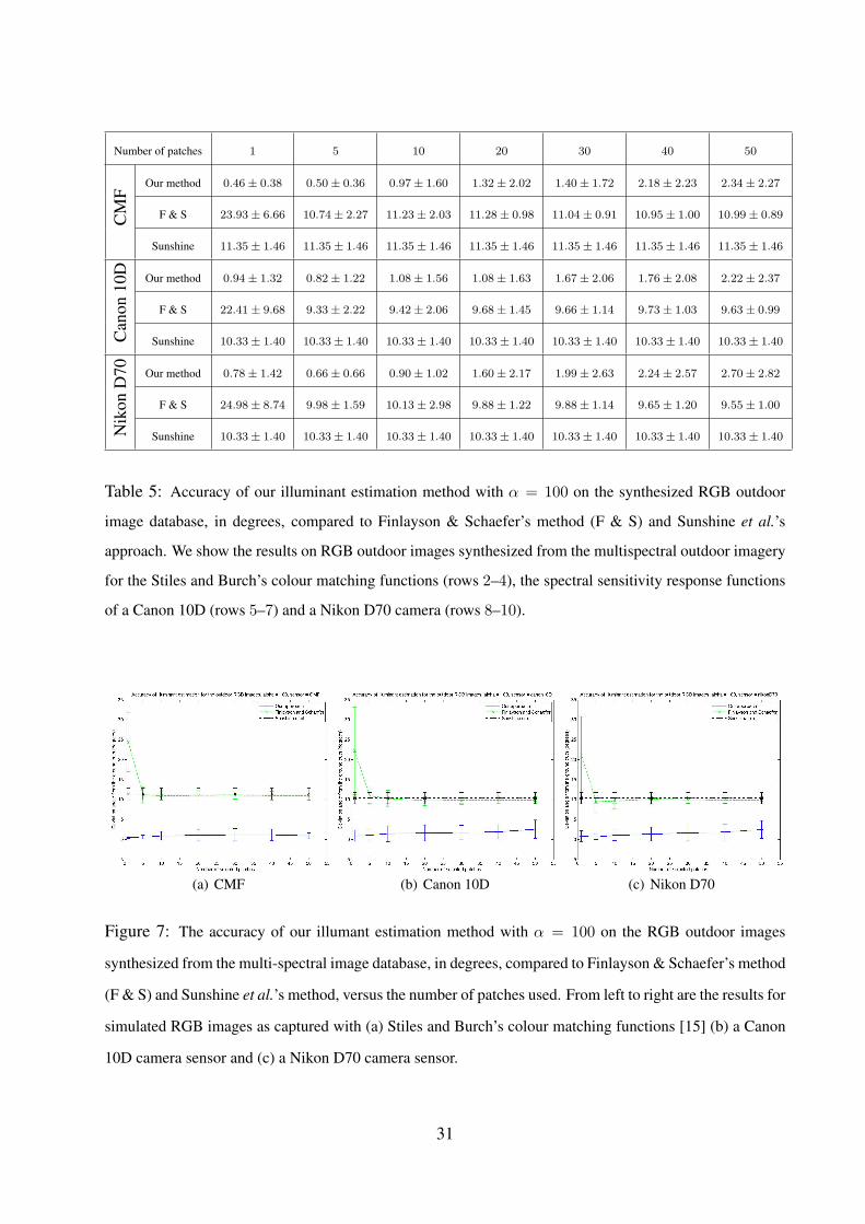
Table 5 and Figure 7 show the accuracy of the illuminant colour estimation on the outdoor RGB

image database, with α = 100 and a patch size of 20 × 20 pixels. The major trend of these

statistics is that our method achieves an accuracy significantly higher than those achieved by the

others. The difference in performance is in the order of several standard deviations of the angular

29

Number of patches 1 5 10 20 30 40 50C

MF

Our method 3.84± 2.86 4.18± 2.89 4.16± 2.79 3.99± 2.61 3.94± 2.58 3.84± 2.54 3.83± 2.55

F & S 24.97± 10.29 5.58± 4.68 4.50± 3.72 3.88± 3.15 3.70± 3.04 3.66± 3.02 3.59± 2.99

Sunshine 6.09± 2.60 6.09± 2.60 6.09± 2.60 6.09± 2.60 6.09± 2.60 6.09± 2.60 6.09± 2.60

Can

on10

D Our method 3.91± 2.87 4.34± 3.01 4.15± 2.72 4.09± 2.52 3.98± 2.45 3.90± 2.36 3.86± 2.34

F & S 25.37± 10.81 3.72± 3.00 3.22± 2.17 2.82± 1.70 2.62± 1.46 2.54± 1.40 2.46± 1.35

Sunshine 5.84± 2.06 5.84± 2.06 5.84± 2.06 5.84± 2.06 5.84± 2.06 5.84± 2.06 5.84± 2.06

Nik

onD

70 Our method 3.88± 2.82 4.26± 2.88 4.17± 2.88 3.91± 2.49 3.93± 2.46 3.85± 2.41 3.86± 2.40

F & S 25.67± 10.83 4.26± 3.94 3.22± 2.30 2.74± 1.67 2.59± 1.50 2.48± 1.37 2.43± 1.31

Sunshine 5.84± 2.06 5.84± 2.06 5.84± 2.06 5.84± 2.06 5.84± 2.06 5.84± 2.06 5.84± 2.06

Table 4: Accuracy of our illuminant estimation method with α = 10000 on the synthesized RGB face

image database, in degrees, compared to Finlayson and Schaefer’s method (F & S) and Sunshine et al.’s

approach. We show the results on RGB face images synthesized from the multispectral face imagery for

the Stiles and Burch’s colour matching functions (rows 2–4), the spectral sensitivity response functions of a

Canon 10D (rows 5–7) and a Nikon D70 camera (rows 8–10).

(a) CMF (b) Canon 10D (c) Nikon D70

Figure 6: Accuracy versus number of image patches for our illuminant estimation method with α = 10000

on the RGB face images synthesized from the multi-spectral face imagery, in degrees, compared to Finlayson

and Schaefer’s method (F & S) and Sunshine et al.’s approach. From left to right: Results for simulated

RGB images as captured with (a) Stiles and Burch’s colour matching functions (b) a Canon 10D camera

sensor (c) a Nikon D70 camera sensor.

error. While the performance of our method is slightly degraded as the number of patch increases

(above 20), the stability of the estimate remains constant for Canon 10D and Nikon D70 images,

and even improves for the images simulated for the CIE 1932 standard colour matching functions.

30

Number of patches 1 5 10 20 30 40 50

CM

F

Our method 0.46± 0.38 0.50± 0.36 0.97± 1.60 1.32± 2.02 1.40± 1.72 2.18± 2.23 2.34± 2.27

F & S 23.93± 6.66 10.74± 2.27 11.23± 2.03 11.28± 0.98 11.04± 0.91 10.95± 1.00 10.99± 0.89

Sunshine 11.35± 1.46 11.35± 1.46 11.35± 1.46 11.35± 1.46 11.35± 1.46 11.35± 1.46 11.35± 1.46

Can

on10

D Our method 0.94± 1.32 0.82± 1.22 1.08± 1.56 1.08± 1.63 1.67± 2.06 1.76± 2.08 2.22± 2.37

F & S 22.41± 9.68 9.33± 2.22 9.42± 2.06 9.68± 1.45 9.66± 1.14 9.73± 1.03 9.63± 0.99

Sunshine 10.33± 1.40 10.33± 1.40 10.33± 1.40 10.33± 1.40 10.33± 1.40 10.33± 1.40 10.33± 1.40

Nik

onD

70 Our method 0.78± 1.42 0.66± 0.66 0.90± 1.02 1.60± 2.17 1.99± 2.63 2.24± 2.57 2.70± 2.82

F & S 24.98± 8.74 9.98± 1.59 10.13± 2.98 9.88± 1.22 9.88± 1.14 9.65± 1.20 9.55± 1.00

Sunshine 10.33± 1.40 10.33± 1.40 10.33± 1.40 10.33± 1.40 10.33± 1.40 10.33± 1.40 10.33± 1.40

Table 5: Accuracy of our illuminant estimation method with α = 100 on the synthesized RGB outdoor

image database, in degrees, compared to Finlayson & Schaefer’s method (F & S) and Sunshine et al.’s

approach. We show the results on RGB outdoor images synthesized from the multispectral outdoor imagery

for the Stiles and Burch’s colour matching functions (rows 2–4), the spectral sensitivity response functions

of a Canon 10D (rows 5–7) and a Nikon D70 camera (rows 8–10).

(a) CMF (b) Canon 10D (c) Nikon D70

Figure 7: The accuracy of our illumant estimation method with α = 100 on the RGB outdoor images

synthesized from the multi-spectral image database, in degrees, compared to Finlayson & Schaefer’s method

(F & S) and Sunshine et al.’s method, versus the number of patches used. From left to right are the results for

simulated RGB images as captured with (a) Stiles and Burch’s colour matching functions [15] (b) a Canon

10D camera sensor and (c) a Nikon D70 camera sensor.

31

No. Standard dynamic range (8 bits) Extended dynamic range (16 bits)


1 8.45± 6.97 25.58± 13.72 12.92± 9.23 8.78± 7.86 24.70± 13.61 12.45± 8.67

5 7.78± 6.23 9.88± 10.71 8.63± 7.75 12.85± 11.90

10 7.78± 6.46 10.06± 10.89 8.18± 7.18 11.73± 11.00

20 7.77± 6.69 9.41± 9.70 7.88± 7.04 10.58± 9.81

30 7.75± 6.90 9.29± 9.76 7.92± 7.03 10.30± 9.57

40 7.82± 6.81 9.12± 9.41 7.81± 7.03 10.18± 9.54

50 7.88± 6.77 9.25± 9.54 7.75± 6.84 10.16± 9.46

Table 6: Accuracy of our illuminant estimation method with α = 1000 on the Mondrian and specular

datasets reported in [4], in degrees, compared to Finlayson and Schaefer’s method (F & S) and Sunshine et

al.’s approach. The accuracy is measured in degrees.

0 10 20 30 40 50−5

0

5

10

15

20

25

30

35

40

Number of selected patches

Dev

iatio

n an

gle

from

the

grou

nd tr

uth

(deg

rees

)

Accuracy of illuminant estimation for the Mondrian and specular datasets, alpha = 1000

Our approachFinlayson and SchaeferSunshine et al.

(a) Standard dynamic range (8 bits)

0 10 20 30 40 500

5

10

15

20

25

30

35

40

Number of selected patches

Dev

iatio

n an

gle

from

the

grou

nd tr

uth

(deg

rees

)

Accuracy of illuminant estimation for the Mondrian and specular datasets, alpha = 1000

Our approachFinlayson and SchaeferSunshine et al.

(b) Extended dynamic range (16 bits)

Figure 8: Accuracy of our illuminant estimation method with α = 1000 for the Mondrian and specu-

lar datasets with 8-bit and 16-bit dynamic ranges, as reported in [4]. Our method is compared to that of

Finlayson and Schaefer (F & S) and Sunshine et al..

It is also important to notice that our method performs better on the imagery synthetised using the

CIE 1932 standard. This is consistent with the results reported for the RGB face images. Overall,

our method appears to outperform the alternatives when applied to cluttered scenes with a high

variation in colour and texture.

Next, we turn our attention to the illuminant estimation accuracy on the Mondrian and specular

image datasets reported in [4]. To account for the level of texture density in some of the images,

32

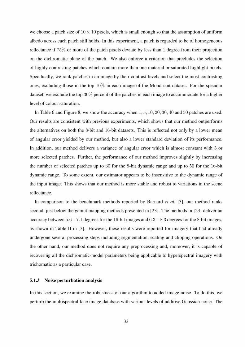
we choose a patch size of 10× 10 pixels, which is small enough so that the assumption of uniform

albedo across each patch still holds. In this experiment, a patch is regarded to be of homogeneous

reflectance if 75% or more of the patch pixels deviate by less than 1 degree from their projection

on the dichromatic plane of the patch. We also enforce a criterion that precludes the selection

of highly contrasting patches which contain more than one material or saturated highlight pixels.

Specifically, we rank patches in an image by their contrast levels and select the most contrasting

ones, excluding those in the top 10% in each image of the Mondriant dataset. For the specular

dataset, we exclude the top 30% percent of the patches in each image to accommodate for a higher

level of colour saturation.

In Table 6 and Figure 8, we show the accuracy when 1, 5, 10, 20, 30, 40 and 50 patches are used.

Our results are consistent with previous experiments, which shows that our method outperforms

the alternatives on both the 8-bit and 16-bit datasets. This is reflected not only by a lower mean

of angular error yielded by our method, but also a lower standard deviation of its performance.

In addition, our method delivers a variance of angular error which is almost constant with 5 or

more selected patches. Further, the performance of our method improves slightly by increasing

the number of selected patches up to 30 for the 8-bit dynamic range and up to 50 for the 16-bit

dynamic range. To some extent, our estimator appears to be insensitive to the dynamic range of

the input image. This shows that our method is more stable and robust to variations in the scene

reflectance.

In comparison to the benchmark methods reported by Barnard et al. [3], our method ranks

second, just below the gamut mapping methods presented in [23]. The methods in [23] deliver an

accuracy between 5.6 – 7.1 degrees for the 16-bit images and 6.3 – 8.3 degrees for the 8-bit images,

as shown in Table II in [3]. However, these results were reported for imagery that had already

undergone several processing steps including segmentation, scaling and clipping operations. On

the other hand, our method does not require any preprocessing and, moreover, it is capable of

recovering all the dichromatic-model parameters being applicable to hyperspectral imagery with

trichomatic as a particular case.

5.1.3 Noise perturbation analysis

In this section, we examine the robustness of our algorithm to added image noise. To do this, we

perturb the multispectral face image database with various levels of additive Gaussian noise. The

33

0.5 1 1.5 2 2.5 32

4

6

8

10

12

14

16

18

Noise level (percentage of the maximum brightness)

Ang

ular

dev

iatio

n fr

om th

e gr

ound

trut

h

Light estimation error (visible range) versus noise level.

Our methodF & SSunshine et al.

(a) Visible spectrum

0.5 1 1.5 2 2.5 30

5

10

15

20

25

Noise level (percentage of the maximum brightness)

Ang

ular

dev

iatio

n fr

om th

e gr

ound

trut

h

Light estimation error (infra−red range) versus noise level.

Our methodF & SSunshine et al.

(b) Infra-red spectrum

Figure 9: Accuracy of the estimated illuminant spectra versus the standard deviation of Gaussian noise.

The vertical axis shows the angular deviation of the estimated spectra from the corresponding ground-truth,

while the horizontal axis shows the standard deviation of Gaussian noise as the percentage of maximum

brightness of the imagery. The performance for the visible spectrum is shown in the left-hand image, while

that corresponding to the infra-red spectrum is shown on the right-hand panel.

noise has an increasing standard deviation between 0.5 and 2% of the maximum image brightness,

with increments of 0.5%. In Figure 9, we plot the performance of our algorithm and the alternatives

across various levels of noise, in the visible (left-hand panel) and infra-red (right-hand panel)

ranges. For our algorithm and Finlayson and Schaefer’s one [21], we employ all the homogenous

patches recovered from the images. The regularisation weight for our method is α = 100000. As

shown in Figure 9, our method achieves a lower mean and standard deviation of the angular error

than the other two in the visible spectrum. Moreover, in the infra-red spectrum, our method greatly

outperforms Sunshine et al.’s [53] by more than two standard deviations of the angular error in the

recovered illuminant spectra.

On the degradation in performance with an increasing level of noise, the Sunshine et al.’s method

is most stable because it considers the upper bound of all the radiance spectra in an image, which

is least affected by the level of Gaussian noise. However, it is the least accurate method of the

three alternatives. Ours and Finlayson & Schaefer’s appear to degrade linearly with the level of

noise, although the latter one degrades at a slower rate than our method. This can be explained

by the fact that Finlayson & Schaefer’s method relies on an eigenvalue decomposition, which is

equivalent to our method with a zero-regularisation term. Albeit obtaining a more robust solution

for the illuminant, their method does not take surface shading and highlights into account. Not

34

only can our approach estimate the illuminant spectrum, it is also capable of computing all the

dichromatic parameters, while maintaining a reasonable estimation using regularisation.

5.2 Skin Recognition and Material Clustering

We now turn our attention to the illumination invariance of the spectral reflectance recovered by our

algorithm and its applications to recognition tasks. Firstly, we focus on using the spectral image

reflectance extracted according to Section 2.4 for skin recognition. This task can be viewed as a

classification problem where the skin and non skin spectra comprise positive and negative classes,

respectively. In this manner, we can assert the robustness and consistency of both the illuminant

spectrum and surface reflectance recovered by our algorithm at training time, and those yielded by

the method for skin recognition at the testing phase.

In this experiment, we compare the skin recognition performance yielded using the reflectance

spectra recovered by our method as the feature for classification to those results yielded by the

classifier using a number of alternative features. To this end, we present the results for two variants

of our recovered reflectance, both estimated by the procedure described in Section 2.4. For the

first variant, the ground-truth illuminant spectrum is supplied as input. For the second one, we use

the estimated illuminant spectra obtained by the experiments in Section 5.1.1. By comparing the

performance in these two cases, we can assess the robustness of the recovered reflectance when

the estimated illuminant spectra is used as compared to the ground-truth. In addition, we also

compare these variants with a number of alternatives. The first of these is the spectral reflectance

obtained by normalising the raw image radiance spectra by the measured ground-truth illuminant.

The second case is where the classifier is applied to the raw radiance spectra. Lastly, we use

the principal components resulting from performing subspace projection via Linear Discriminant

Analysis (LDA) on the original radiance spectra.

This experiment is performed on the face image database captured in the visible range described

earlier. To obtain a training data-set, we select skin and non skin regions from an image captured

under a light source placed in a high-oblique position in front of the subject. On average, there are

856 skin pixels and 7796 non-skin pixels selected from several regions in each image as training

data. Subsequently, each of the features described above is extracted from each training set and

used as input to a Support Vector Machine (SVM) classifier [13] with a Radial Basis Function

(RBF) kernel. In addition, the parameters are selected using 5-fold cross validation at training

35

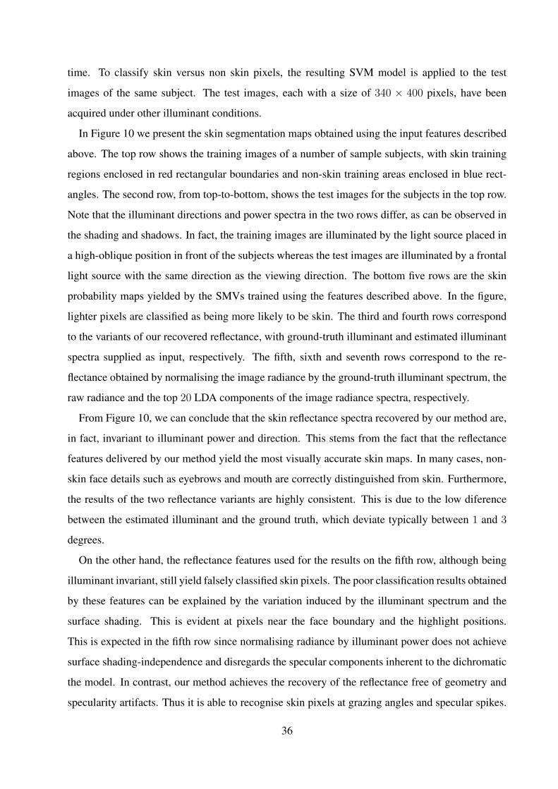
time. To classify skin versus non skin pixels, the resulting SVM model is applied to the test

images of the same subject. The test images, each with a size of 340 × 400 pixels, have been

acquired under other illuminant conditions.

In Figure 10 we present the skin segmentation maps obtained using the input features described

above. The top row shows the training images of a number of sample subjects, with skin training

regions enclosed in red rectangular boundaries and non-skin training areas enclosed in blue rect-

angles. The second row, from top-to-bottom, shows the test images for the subjects in the top row.

Note that the illuminant directions and power spectra in the two rows differ, as can be observed in

the shading and shadows. In fact, the training images are illuminated by the light source placed in

a high-oblique position in front of the subjects whereas the test images are illuminated by a frontal

light source with the same direction as the viewing direction. The bottom five rows are the skin

probability maps yielded by the SMVs trained using the features described above. In the figure,

lighter pixels are classified as being more likely to be skin. The third and fourth rows correspond

to the variants of our recovered reflectance, with ground-truth illuminant and estimated illuminant

spectra supplied as input, respectively. The fifth, sixth and seventh rows correspond to the re-

flectance obtained by normalising the image radiance by the ground-truth illuminant spectrum, the

raw radiance and the top 20 LDA components of the image radiance spectra, respectively.

From Figure 10, we can conclude that the skin reflectance spectra recovered by our method are,

in fact, invariant to illuminant power and direction. This stems from the fact that the reflectance

features delivered by our method yield the most visually accurate skin maps. In many cases, non-

skin face details such as eyebrows and mouth are correctly distinguished from skin. Furthermore,

the results of the two reflectance variants are highly consistent. This is due to the low diference

between the estimated illuminant and the ground truth, which deviate typically between 1 and 3

degrees.

On the other hand, the reflectance features used for the results on the fifth row, although being

illuminant invariant, still yield falsely classified skin pixels. The poor classification results obtained

by these features can be explained by the variation induced by the illuminant spectrum and the

surface shading. This is evident at pixels near the face boundary and the highlight positions.

This is expected in the fifth row since normalising radiance by illuminant power does not achieve

surface shading-independence and disregards the specular components inherent to the dichromatic

the model. In contrast, our method achieves the recovery of the reflectance free of geometry and

specularity artifacts. Thus it is able to recognise skin pixels at grazing angles and specular spikes.

36

Figure 10: Skin segmentation results. Top row: sample training images for skin recognition, with labelled

skin regions (with red borders) and non-skin regions (in blue borders). Second row: the test images of the

corresponding subjects, captured under a different illumination direction. The third to last row are the skin

probability map obtained using different features. Third row: obtained using the reflectance estimated given

the ground-truth illuminant spectrum. Fourth row: yielded using the estimated reflectance after estimating

the illuminant spectrum. Fifth row: yielded using the reflectance obtained by normalising radiance spectra

by the ground-truth illuminant spectrum. Sixth row: yielded using the raw radiance of the input images.

Seventh row: recovered making use of the top 20 LDA components of the raw radiance spectra.

37

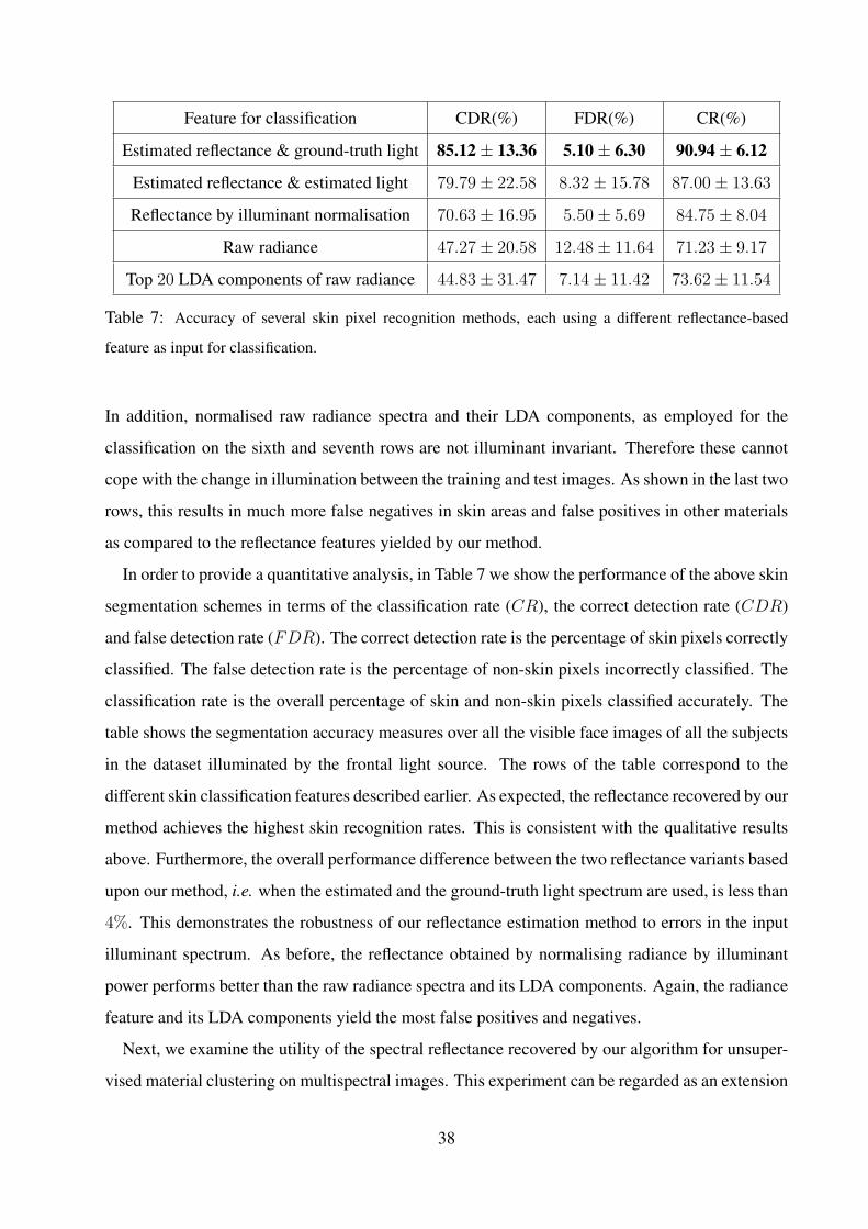
Feature for classification CDR(%) FDR(%) CR(%)

Estimated reflectance & ground-truth light 85.12± 13.36 5.10± 6.30 90.94± 6.12

Estimated reflectance & estimated light 79.79± 22.58 8.32± 15.78 87.00± 13.63

Reflectance by illuminant normalisation 70.63± 16.95 5.50± 5.69 84.75± 8.04

Raw radiance 47.27± 20.58 12.48± 11.64 71.23± 9.17

Top 20 LDA components of raw radiance 44.83± 31.47 7.14± 11.42 73.62± 11.54

Table 7: Accuracy of several skin pixel recognition methods, each using a different reflectance-based

feature as input for classification.

In addition, normalised raw radiance spectra and their LDA components, as employed for the

classification on the sixth and seventh rows are not illuminant invariant. Therefore these cannot

cope with the change in illumination between the training and test images. As shown in the last two

rows, this results in much more false negatives in skin areas and false positives in other materials

as compared to the reflectance features yielded by our method.

In order to provide a quantitative analysis, in Table 7 we show the performance of the above skin

segmentation schemes in terms of the classification rate (CR), the correct detection rate (CDR)

and false detection rate (FDR). The correct detection rate is the percentage of skin pixels correctly

classified. The false detection rate is the percentage of non-skin pixels incorrectly classified. The

classification rate is the overall percentage of skin and non-skin pixels classified accurately. The

table shows the segmentation accuracy measures over all the visible face images of all the subjects

in the dataset illuminated by the frontal light source. The rows of the table correspond to the

different skin classification features described earlier. As expected, the reflectance recovered by our

method achieves the highest skin recognition rates. This is consistent with the qualitative results

above. Furthermore, the overall performance difference between the two reflectance variants based

upon our method, i.e. when the estimated and the ground-truth light spectrum are used, is less than

4%. This demonstrates the robustness of our reflectance estimation method to errors in the input

illuminant spectrum. As before, the reflectance obtained by normalising radiance by illuminant

power performs better than the raw radiance spectra and its LDA components. Again, the radiance

feature and its LDA components yield the most false positives and negatives.

Next, we examine the utility of the spectral reflectance recovered by our algorithm for unsuper-

vised material clustering on multispectral images. This experiment can be regarded as an extension

38

Figure 11: Material clusters, with each material marked by a different shade of gray. Top row: A band

of the input images, shown at 670 nm. Second row: material clustering maps, obtained with the clustering

feature being the estimated reflectance given the ground-truth illuminant. Third row: material clustering

maps resulting from the use of the reflectance feature recovered with an estimated illuminant spectrum as

input. Fourth row: material clustering maps, using the reflectance obtained by normalising the input radiance

image by the ground-truth illuminant spectrum.

of the skin segmentation application. In addition, it is complementary to skin clustering algorithms

using trichromatic features, which has been described elsewhere in the literature [44]. It also

compares the clustering accuracy on the estimated reflectance to that on the measured (ground-

truth) reflectance. Here, we perform a clustering algorithm based on a deterministic annealing

approach [27] on the three reflectance features mentioned in the previous experiment. These fea-

tures include the estimated reflectance estimated given the ground-truth illuminant spectrum, the

estimated reflectance yielded from an estimated illuminant spectrum, and the reflectance obtained

by normalising radiance spectra by the ground-truth illuminant spectrum. The clustering algorithm

is initialised with a single cluster for all the materials. As the algorithm proceeds, new material

clusters are introduced by splitting the existing ones. Thus, the resulting number of clusters is

39

data-dependent and does not need to be specified as input.

In Figure 11, we show the clustering maps of the images of several human subjects, with each

row corresponding to a reflectance feature. The resulting material clusters are marked with differ-

ent shades of gray. In fact, there are a high level of similarity between the clutering results yielded

by the reflectance features estimated with the estimated illumant spectrum and with the ground

truth illuminant spectrum provided as input, as shown in rows 2 and 3. This demonstrates, again,

the robustness of our reflectance estimation method to errors in the input illuminant spectrum. In

these clustering maps, all the materials are well-separated from each other. Moreover, there are

very few misclassified pixels within each cluster. On the faces, the skin pixels are clearly distin-

guished from the neighbouring regions. Notably, the background regions displaying printed faces,

such as that in the third column, are correctly clustered as paper. This result demonstrates that

the spectral variation of material reflectance is a better feature for classification than trichromatic

colour. Note that using trichromatic imagery, it would have been virtually impossible to set apart

materials with the same apparent color, such as real faces from printed ones. In the last row, we

use the ground truth (measured) reflectance as feature for the clustering algorithm. Compared to

our estimated reflectance, the measured reflectance produces noisier clustering maps, with a sub-

stantial number of pixels made of the same material assigned to various clusters. In other words,

our reflectance recovery method improves the clustering performance by reducing measurement

noise in the raw reflectance spectra.

5.3 Specularity Removal

Having estimated the illuminant spectra and surface reflectance, and as mentioned previously, we

can employ the procedure in Section 2.4 to separate the diffuse from the specular component in

multi-spectral imagery. This is feasible in situations where the spectral reflectance varies slowly

within a small spatial neighbourhood of the scene. Note that this assumption is a valid one for many

real-world surfaces. Thus, each local neighbourhood can be considered as a smooth homogeneous

surface. As a result, the diffuse component at a location u in patch P is estimated as D(u) =

g(u)(L • SP ). The specularity component is given by k(u)L.

Here, we perform highlight removal on the indoor human face image database presented ear-

lier. As mentioned in previous sections, we commence by estimating the illuminant spectra. We

consider a neighbourhood of size 11× 11 around each image pixel and assume that the neighbour-

40

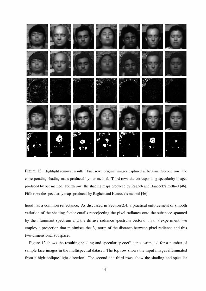
Figure 12: Highlight removal results. First row: original images captured at 670nm. Second row: the

corresponding shading maps produced by our method. Third row: the corresponding specularity images

produced by our method. Fourth row: the shading maps produced by Ragheb and Hancock’s method [46].

Fifth row: the specularity maps produced by Ragheb and Hancock’s method [46].

hood has a common reflectance. As discussed in Section 2.4, a practical enforcement of smooth

variation of the shading factor entails reprojecting the pixel radiance onto the subspace spanned

by the illuminant spectrum and the diffuse radiance spectrum vectors. In this experiment, we

employ a projection that minimises the L2-norm of the distance between pixel radiance and this

two-dimensional subspace.

Figure 12 shows the resulting shading and specularity coefficients estimated for a number of

sample face images in the multispectral dataset. The top row shows the input images illuminated

from a high oblique light direction. The second and third rows show the shading and specular

41

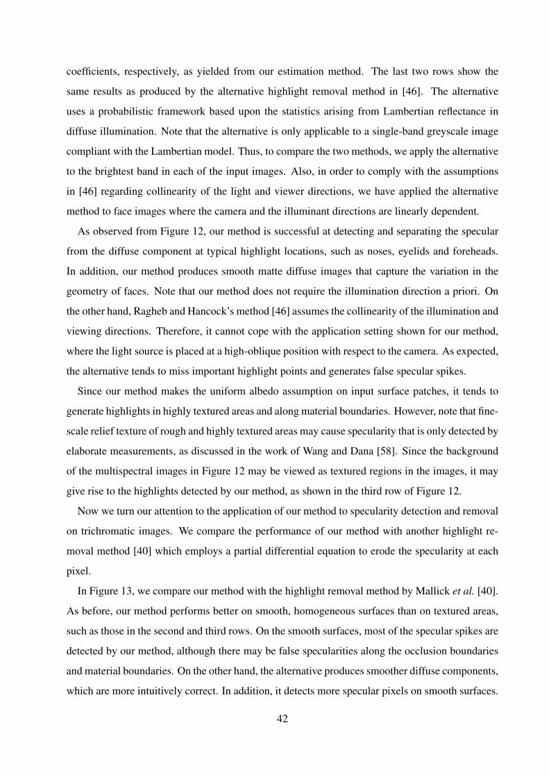
coefficients, respectively, as yielded from our estimation method. The last two rows show the

same results as produced by the alternative highlight removal method in [46]. The alternative

uses a probabilistic framework based upon the statistics arising from Lambertian reflectance in

diffuse illumination. Note that the alternative is only applicable to a single-band greyscale image

compliant with the Lambertian model. Thus, to compare the two methods, we apply the alternative

to the brightest band in each of the input images. Also, in order to comply with the assumptions

in [46] regarding collinearity of the light and viewer directions, we have applied the alternative

method to face images where the camera and the illuminant directions are linearly dependent.

As observed from Figure 12, our method is successful at detecting and separating the specular

from the diffuse component at typical highlight locations, such as noses, eyelids and foreheads.

In addition, our method produces smooth matte diffuse images that capture the variation in the

geometry of faces. Note that our method does not require the illumination direction a priori. On

the other hand, Ragheb and Hancock’s method [46] assumes the collinearity of the illumination and

viewing directions. Therefore, it cannot cope with the application setting shown for our method,

where the light source is placed at a high-oblique position with respect to the camera. As expected,

the alternative tends to miss important highlight points and generates false specular spikes.

Since our method makes the uniform albedo assumption on input surface patches, it tends to

generate highlights in highly textured areas and along material boundaries. However, note that fine-

scale relief texture of rough and highly textured areas may cause specularity that is only detected by

elaborate measurements, as discussed in the work of Wang and Dana [58]. Since the background

of the multispectral images in Figure 12 may be viewed as textured regions in the images, it may

give rise to the highlights detected by our method, as shown in the third row of Figure 12.

Now we turn our attention to the application of our method to specularity detection and removal

on trichromatic images. We compare the performance of our method with another highlight re-

moval method [40] which employs a partial differential equation to erode the specularity at each

pixel.

In Figure 13, we compare our method with the highlight removal method by Mallick et al. [40].

As before, our method performs better on smooth, homogeneous surfaces than on textured areas,

such as those in the second and third rows. On the smooth surfaces, most of the specular spikes are

detected by our method, although there may be false specularities along the occlusion boundaries

and material boundaries. On the other hand, the alternative produces smoother diffuse components,

which are more intuitively correct. In addition, it detects more specular pixels on smooth surfaces.

42

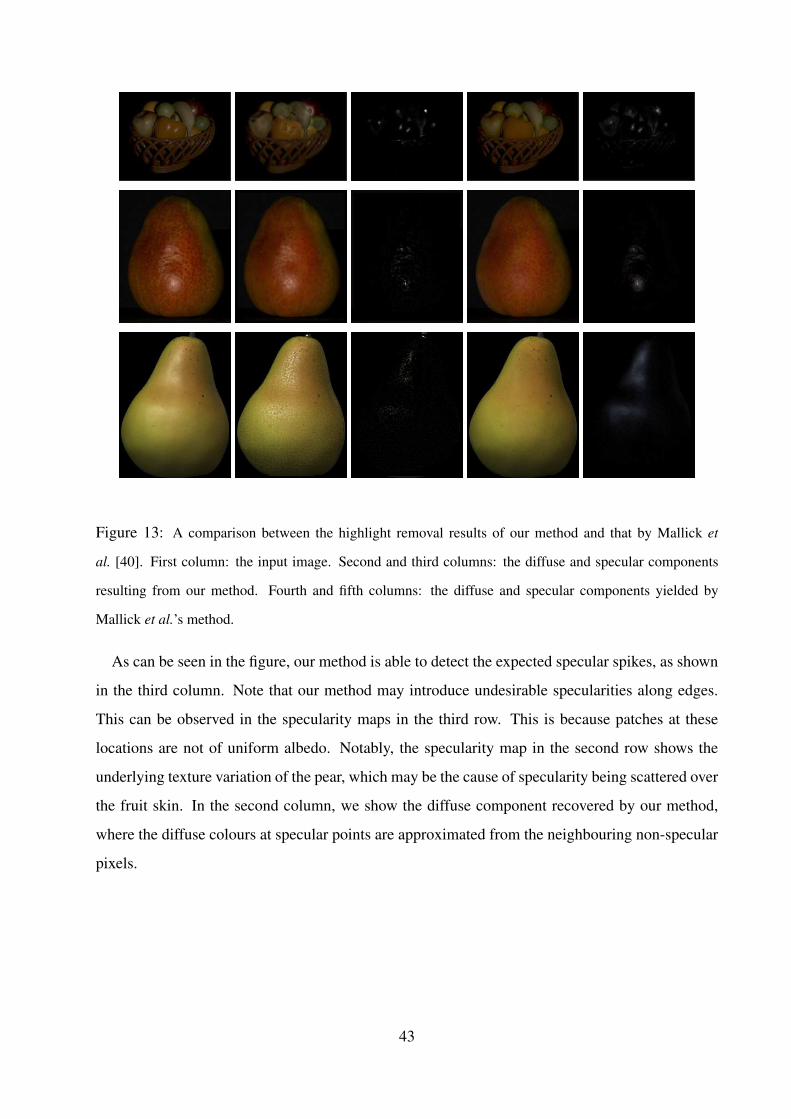
Figure 13: A comparison between the highlight removal results of our method and that by Mallick et

al. [40]. First column: the input image. Second and third columns: the diffuse and specular components

resulting from our method. Fourth and fifth columns: the diffuse and specular components yielded by

Mallick et al.’s method.

As can be seen in the figure, our method is able to detect the expected specular spikes, as shown

in the third column. Note that our method may introduce undesirable specularities along edges.

This can be observed in the specularity maps in the third row. This is because patches at these

locations are not of uniform albedo. Notably, the specularity map in the second row shows the

underlying texture variation of the pear, which may be the cause of specularity being scattered over

the fruit skin. In the second column, we show the diffuse component recovered by our method,

where the diffuse colours at specular points are approximated from the neighbouring non-specular

pixels.

43

6 Conclusions

In this paper, we have presented an optimisation approach so as to recover a solution to the dichro-

matic model for purposes of photometric invariance from a single multispectral image. The re-

covery process is based upon optimising a cost function that imposes a smoothness constraint

on dichromatic surfaces with uniform reflectance. The method serves several purposes, including

scene illuminant estimation, reflectance-based recognition and clustering, and specularity removal.

Departing from the dichromatic model, we have presented a cost function which can be optimised

using a coordinate descent approach applied to automatically selected surface patches. We have

also elaborated upon the use of a number of regularisation strategies so as to enforce smoothness

constraints upon the cost function. The method is, hence, quite general in nature, and it is not

limited to hyperspectral imagery and is applicable to trichromatic imagery in a straightforward

manner. We have shown experiments on real-world imagery where, firstly, the illuminant spectra

resulting from our method are shown to outperform those delivered by the alternative methods, es-

pecially with a small number of selected homogeneous surface patches. Secondly, we have shown

how the reflectance spectra recovered by our method can used for skin recognition and material

clustering purposes. Finally, we have shown how specularities can be removed from surfaces to

facilitate further computer vision tasks.

References

[1] ANGELOPOULOU, E. Objective colour from multispectral imaging. In European Conf. on Computer

Vision (2000), pp. 359–374.

[2] ANGELOPOULOU, E. Specular highlight detection based on the fresnel reflection coefficient. In

IEEE International Conference on Computer Vision (Los Alamitos, CA, USA, 2007), IEEE Computer

Society, pp. 1–8.

[3] BARNARD, K., MARTIN, L., COATH, A., AND FUNT, B. V. A comparison of computational color

constancy Algorithms – Part II: Experiments with image data. IEEE Transactions on Image Processing

11, 9 (2002), 985–996.

[4] BARNARD, K., MARTIN, L., FUNT, B., AND COATH, A. A Data Set for Colour Research. Color

Research and Application 27, 3 (2002), 147–151.

[5] BARNARD, K., MARTIN, L., AND FUNT, B. V. Colour by Correlation in a Three-Dimensional

Colour Space. In ECCV ’00: Proceedings of the 6th European Conference on Computer Vision-Part I

44

(London, UK, 2000), Springer-Verlag, pp. 375–389.

[6] BOYD, S., AND VANDENBERGHE, L. Convex Optimization. Cambridge University Press, 2004.

[7] BRAINARD, D., AND WANDELL, B. Analysis of the retinex theory of color vision. Journal of Optical

Society America A 3 (1986), 1651–1661.

[8] BRAINARD, D. H., DELAHUNT, P. B., FREEMAN, W. T., KRAFT, J. M., AND XIAO, B. Bayesian

model of human color constancy. Journal of Vision 6, 11 (2006), 1267–1281.

[9] BRAINARD, D. H., AND FREEMAN, W. T. Bayesian color constancy. Journal of Optical Society

America A 14, 7 (1997), 1393–1411.

[10] BRELSTAFF, G., AND BLAKE, A. Detecting specular reflection using lambertian constraints. In Int.

Conf. on Comp. Vision (1988), pp. 297–302.

[11] BROOKS, M., AND HORN, B. Shape and source from shading. In MIT AI Memo (1985).

[12] BUCHSBAUM, G. A Spatial Processor Model for Object Color Perception. Journal of The Franklin

Institute 310 (1980), 1–26.

[13] CHANG, C.-C., AND LIN, C.-J. LIBSVM: a library for Support Vector Machines, 2001.

[14] CHANG, J. Y., LEE, K. M., AND LEE, S. U. Shape from shading using graph cuts. In Proc. of the

Int. Conf. on Image Processing (2003).

[15] CIE. Commission Internationale de l’Eclairage Proceedings, 1931. Cambridge University Press,

Cambridge, 1932.

[16] DROR, R. O., ADELSON, E. H., AND WILLSKY, A. S. Recognition of Surface Reflectance Properties

from a Single Image under Unknown Real-World Illumination. In Proc. of the IEEE Workshop on

Identifying Objects Across Variations in Lighting (2001).

[17] FERRIE, F., AND LAGARDE, J. Curvature consistency improves local shading analysis. CVGIP:

Image Understanding 55, 1 (1992), 95–105.

[18] FINLAYSON, G., AND HORDLEY, S. Improving Gamut Mapping Color Constancy. IEEE Transac-

tions on Image Processing 9, 10 (2000).

[19] FINLAYSON, G. D., HORDLEY, S. D., AND HUBEL, P. M. Color by Correlation: A Simple, Unifying

Framework for Color Constancy. IEEE Transactions on Pattern Analysis and Machine Intelligence 23,

11 (2001), 1209–1221.

[20] FINLAYSON, G. D., HORDLEY, S. D., AND TASTL, I. Gamut constrained illuminant estimation. Int.

J. Comput. Vision 67, 1 (2006), 93–109.

[21] FINLAYSON, G. D., AND SCHAEFER, G. Convex and Non-convex Illuminant Constraints for Dichro-

matic Colour Constancy. CVPR 1 (2001), 598–604.

[22] FINLAYSON, G. D., AND SCHAEFER, G. Solving for Colour Constancy using a Constrained Dichro-

matic Reflection Model. International Journal of Computer Vision 42, 3 (2001), 127–144.

45

[23] FORSYTH, D. A. A novel algorithm for color constancy. International Journal of Computer Vision 5,

1 (1990), 5–36.

[24] HEALEY, G. Estimating spectral reflectance using highlights. Image and Vision Computing 9, 5

(October 1991), 333–337.

[25] HEALEY, G., AND SLATER, D. Invariant recognition in hyperspectral images. In IEEE Conf. on

Computer Vision and Pattern Recognition (1999), pp. 1438–1043.

[26] HOAGLIN, D. C., MOSTELLER, F., AND TUKEY, J. W. Understanding Robust and Exploratory Data

Analysis. Wiley-Interscience, 2000.

[27] HOFMANN, T., AND BUHMANN, M. Pairwise data clustering by deterministic annealing. IEEE

Tansactions on Pattern Analysis and Machine Intelligence 19, 1 (1997), 1–14.

[28] HORN, B. K. P. Robot Vision. MIT Press, Cambridge, Massachusetts, 1986.

[29] HORN, B. K. P., AND BROOKS, M. J. The variational approach to shape from shading. CVGIP 33, 2

(1986), 174–208.

[30] HUBER, P. J. Robust Statistics. Wiley-Interscience, 1981.

[31] IKEUCHI, K., AND HORN, B. Numerical shape from shading and occluding boundaries. Artificial

Intelligence 17, 1-3 (August 1981), 141–184.

[32] KLINKER, G., SHAFER, S., AND KANADE, T. A Physical Approach to Color Image Understanding.

International Journal of Computer Vision 4, 1 (1990), 7–38.

[33] KLINKER, G. J., SHAFER, S. A., AND KANADE, T. The Measurement of Highlights in Color Images.

International Journal of Computer Vision 2 (1988), 7–32.

[34] KOENDERINK, J. J., AND VAN DOORN, A. J. Surface shape and curvature scales. Image Vision

Computing 10, 8 (1992), 557–565.

[35] LAND, E., AND MCCANN, J. Lightness and retinex theory. Journal of Optical Society America 61, 1

(1971), 1–11.

[36] LAND, E. H. Recent advances in retinex theory. Vision Research 26, 1 (1986).

[37] LEE, H.-C. Method for computing the scene-illuminant chromaticity from specular highlights. Jour-

nal of the Optical Society of America A 3 (1986), 1694–1699.

[38] LI, S. Z. Discontinuous mrf prior and robust statistics: a comparative study. Image Vision Computing

13, 3 (1995), 227–233.

[39] LIN, S., AND SHUM, H.-Y. Separation of Diffuse and Specular Reflection in Color Images. Computer

Vision and Pattern Recognition, IEEE Computer Society Conference on 1 (2001), 341.

[40] MALLICK, S. P., ZICKLER, T., BELHUMEUR, P. N., AND KRIEGMAN, D. J. Specularity Removal

in Images and Videos: A PDE Approach. In ECCV (1) (2006), pp. 550–563.

[41] NARASIMHAN, S. G., RAMESH, V., AND NAYAR, S. K. A Class of Photometric Invariants: Sepa-

46

rating Material from Shape and Illumination. In International Conference on Computer Vision (Wash-

ington, DC, USA, 2003), IEEE Computer Society, pp. 1387–1394.

[42] NAYAR, S., AND BOLLE, R. Reflectance based object recognition. International Journal of Computer

Vision 17, 3 (1996), 219–240.

[43] NAYAR, S. K., AND BOLLE, R. M. Computing reflectance ratios from an image. Pattern Recognition

26 (1993), 1529–1542.

[44] PHUNG, S. L., BOUZERDOUM, A., AND CHAI, D. Skin segmentation using color pixel classification:

Analysis and comparison. IEEE Trans. Pattern Anal. Mach. Intell. 27, 1 (2005), 148–154.

[45] POGGIO, T., AND TORRE, V. Ill-posed problems and regularization analysis in early vision. Tech.

rep., Cambridge, MA, USA, 1984.

[46] RAGHEB, H., AND HANCOCK, E. R. Highlight removal using shape-from-shading. In European

Conf. on Comp. Vision (2002), no. 2351 in LNCS, pp. 626–641.

[47] RASKAR, R., TUMBLIN, J., MOHAN, A., AGRAWAL, A., AND LI, Y. Computational Photography.

In Proceeding of Eurographics: State of the Art Report (STAR).

[48] SCHAEFER, G., HORDLEY, S., AND FINLAYSON, G. A Combined Physical and Statistical Approach

to Colour Constancy. Computer Vision and Pattern Recognition, IEEE Computer Society Conference

on 1 (2005), 148–153.

[49] SHAFER, S. A. Using color to separate reflection components. Color Research and Applications 10,

4 (1985), 210–218.

[50] SLATER, D., AND HEALEY, G. Object recognition using invariant profiles. In Computer Vision and

Pattern Recognition (1997), pp. 827–832.

[51] STOCKMAN, H., AND GEVERS, T. Detection and classification of hyperspectral edges. In British

Machine Vision Conference (1999), pp. 643–651.

[52] SUEN, P. H., AND HEALEY, G. Invariant mixture recognition in hyperspectral images. In Int. Con-

ference on Computer Vision (2001), pp. 262–267.

[53] SUNSHINE, J. M., PIETERS, C. M., AND PRATT, S. F. Deconvolution of Mineral Absorption Bands:

An Improved Approach. Journal of Geophysical Research 95, B5 (1990), 6955–6966.

[54] TAN, R. T., NISHINO, K., AND IKEUCHI, K. Separating reflection components based on chromaticity

and noise analysis. IEEE Trans. Pattern Anal. Mach. Intell. 26, 10 (2004), 1373–1379.

[55] TOMINAGA, S., AND WANDELL, B. A. Standard surface-reflectance model and illuminant estimation.

Journal of the Optical Society of America A 6 (April 1989), 576–584.

[56] TOMINAGA, S., AND WANDELL, B. A. Component estimation of surface spectral reflectance. Journal

of the Optical Society of America A 7, 2 (February 1990), 312–317.

[57] VAN DE WEIJER, J., AND GEVERS, T. Color constancy based on the grey-edge hypothesis. In IEEE

47

International Conference on Image Processing (2005), vol. 2, pp. 722–725.

[58] WANG, J., AND DANA, K. J. Relief texture from specularities. IEEE Transactions on Pattern Analysis

and Machine Intelligence 28, 3 (2006), 446–457.

[59] WORTHINGTON, P. L., AND HANCOCK, E. R. New constraints on data-closeness and needle map

consistency for shape-from-shading. IEEE Transactions on Pattern Analysis and Machine Intelligence

21, 12 (1999), 1250–1267.

[60] ZHENG, Q., AND CHELLAPA, R. Estimation of illuminant direction, albedo, and shape from shading.

IEEE Transactions on Pattern Analysis and Machine Intelligence 13, 7 (1991), 680–702.

[61] ZICKLER, T., MALLICK, S. P., KRIEGMAN, D. J., AND BELHUMEUR, P. N. Color subspaces as

photometric invariants. International Journal of Computer Vision 79, 1 (2008), 13–30.

48

A solution of the dichromatic model for multispectral photometric invariance

Documents