A soil water and salt balance model Reference Manual Version 5.0 – June 2002 Dirk RAES K.U.Leuven Faculty of Agricultural and Applied Biological Sciences Institute for Land and Water Management Vital Decosterstraat 102, B-3000 LEUVEN, Belgium e-mail: [email protected]

Welcome message from author
This document is posted to help you gain knowledge. Please leave a comment to let me know what you think about it! Share it to your friends and learn new things together.
Transcript
A soil water and salt balance model
Reference Manual Version 5.0 – June 2002 Dirk RAES K.U.Leuven Faculty of Agricultural and Applied Biological Sciences Institute for Land and Water Management Vital Decosterstraat 102, B-3000 LEUVEN, Belgium e-mail: [email protected]
BUDGET – Reference Manual Table of Contents ii
Table of contents Chapter 1. BUDGET 1.1 Input 1.2 Output 1.3 Subroutines 1.4 Installation and structure
1. 2 1. 2 1. 3 1. 4
Chapter 2. Menu Reference 2.1 Main menu 2.2 Climate input (ETo and Rain data) 2.3 Crop data
2.3.1 Select/Create crop file 2.3.2 Crop Parameters
a. Growth stages and Kc coefficients b. Sensitivity stages and Ky coefficients c. Partitioning of ETcrop d. Rooting depth e. Water stress f. Aeration stress g. Water extraction pattern h. Salt tolerance
2.4 Profile description 2.4.1 Select/Create soil file 2.4.2 Soil Parameters
a. Soil layers b. Bunds and surface runoff
2.5 Irrigation options 2.5.1 No irrigation (rainfed agriculture) 2.5.2 Determination of Irrigation water requirement 2.5.3 Irrigation scheduling
a. In crop season b. Out of crop season c. Irrigation water quality
2.6 Simulation Period 2.7 Initial conditions
2.7.1 Initial soil water and salt conditions 2.7.2 Soil cover outside growing period 2.7.3 Cumulative counters
2.8 Output files
2. 1 2. 2 2. 3 2. 3 2. 6 2. 6 2. 7 2. 8 2. 9 2. 9 2.10 2.11 2.12 2.13 2.13 2.14 2.14 2.15 2.16 2.16 2.16 2.16 2.16 2.17 2.17 2.18 2.19 2.19 2.19 2.19 2.20
BUDGET – Reference Manual Table of Contents iii
2.9 Program parameters 2.9.1 Display 2.9.2 Evaporation 2.9.3 Transpiration 2.9.4 Salinity 2.9.5 Surface runoff 2.9.6 Soil compartments 2.9.7 Initial conditions 2.9.8 Irrigation 2.9.9 Effective rainfall
2.10 Run 2.10.1 Input section 2.10.2 Output section 2.10.3 Graphical displays
2.21 2.21 2.21 2.21 2.21 2.22 2.22 2.23 2.23 2.23 2.24 2.24 2.25 2.25
Chapter 3. Calculation procedures 3.1 Simulation of the soil water and salt balance 3.2 Drainage subroutine 3.3 Runoff subroutine 3.4 Infiltration subroutine 3.5 Crop evapotranspiration
3.5.1 Evaporation power of the atmosphere 3.5.2 Partitioning of ETcrop 3.5.3 Evaporation subroutine 3.5.4 Transpiration subroutine 3.5.5 Actual crop evapotranspiration (ETact)
3.6 Estimation of Relative Yield 3.7 Salt transport
3.7.1 Vertical and horizontal salt movement 3.7.2 Cells 3.7.3 Salt diffusion 3.7.4 Soil evaporation 3.7.5 Crop transpiration
3.8 Processing of 10-day and monthly climatic data 3.8.1 Estimation of surface runoff 3.8.2 Estimation of effective rainfall
a. 100 percent effective b. USDA-SCS procedure c. Expressed as a percentage of rainfall
3. 1 3. 4 3. 7 3. 8 3. 9 3. 9 3. 9 3.10 3.10 3.11 3.12 3.13 3.13 3.13 3.15 3.16 3.16 3.18 3.18 3.19 3.19 3.19 3.19

BUDGET – Reference Manual Table of Contents iv
References Annex I. Indicative values for Crop Parameters 1. Lengths of crop development stages 2. Crop coefficients 3. Maximum effective rooting depth and maximum depletion factors 4. Maximum crop salt tolerance levels 5. Yield response factors
I. 2 I. 7 I.12 I.15 I.17
Annex II. Indicative values and pedo-transfer functions
for Hydraulic properties of soil layers 1. Water content at saturation (θsat), field capacity (θFC) and wilting
point (θWP) 2. Saturated hydraulic conductivity (Ksat) 3. Drainage characteristic (τ)
II.1
II.3 II.5

BUDGET – Reference Manual 1. 1
The BUDGET program
BUDGET is composed of a set of validated subroutines describing the various processes involved in water extraction by plant roots and water movement in the soil profile. During periods of crop water stress the resulting yield depression is estimated by means of yield response factors. By selecting appropriate time and depth criteria irrigation schedules can be generated. The climatic data consists of daily, mean 10-day or monthly ETo (reference crop evapotranspiration) and Rainfall observations. At run time, the 10-day and monthly data are processed to derive daily ETo and Rain data. By specifying and selecting a few appropriate crop parameters in a Menu driven environment, the program creates a complete set of parameters that can be displayed and updated if additional information is available. The soil profile may be composed of several soil layers, each with their specific characteristics. BUDGET contains a complete set of default characteristics that can be selected and adjusted for various types of soil layers. By calculating the water and salt content in a soil profile as affected by input and withdrawal of water and salt during the simulation period, the program is suitable: - to asses crop water stress under rainfed conditions; - to estimate yield response to water; - to design irrigation schedules; - to study the building of salt in the root zone under averse irrigation conditions; - to evaluate irrigation strategies. By visualising the variation of the soil water content and the building up of salt in the soil profile during the simulation process, the program is also valuable as a didactic tool.

BUDGET – Reference Manual 1. 2
Chapter 1. BUDGET
1.1 Input The input consists of: 1. daily, 10-day or monthly Climatic data:
- Evaporative demand of the atmosphere (i.e. the Reference evapotranspiration, ETo);
- Rainfall 2. Crop parameters: Parameters describing crop development and root water
uptake. By selecting the appropriate: - Class of Crop type; - Class of rooting depth (from shallow rooted crops to very deep rooted crops); - Class of sensitivity to water stress (from sensitive to water stress to tolerant to
stress); - Class of degree of ground cover at maximum crop canopy (from sparse ground
cover to very dense cover); - and specifying the total length of growing period, BUDGET generates a
complete set of crop parameters. The generated crop parameters can be adjusted;
3. Soil parameters: The soil profile may be composed of several soil layers, each with their specific characteristics. BUDGET contains a complete set of default characteristics which can be selected and adjusted for various types of soil layers;
4. Irrigation data: Water quality (salinity), Irrigation Intervals and water Application Depths or criteria to generate irrigation schedules;
5. Initial soil water and salt conditions in the soil profile; 1.2 Output With the described input and for the given initial conditions, BUDGET simulates the solute transport and water uptake in the specified Climate/Crop/Soil environment and for the specified irrigation option.
1. During the simulation process the variation of the soil water content and salt build up in the profile is visualised by displaying at the end of each day of the simulation period :
- the soil water and salt content at different depths in the soil profile; - the water level in the soil water reservoir; - the root zone depletion.
2. At the end of the simulation process, BUDGET displays: - the final soil moisture profile; - the final salt content of the soil water solution in the soil profile; - the total value for each of the parameters of the soil water balance; - the expected relative crop yield; and - the irrigation water requirement.
3. During the simulation, BUDGET records continuously the daily soil water and salt content in the soil profile, soil water
BUDGET – Reference Manual 1. 3
fluxes, daily values of the various parameters of the soil water and salt balances, the daily root zone depletion and net irrigation requirement. The daily records are stored in various output files, which contents can be displayed at the end of the simulation run with different time aggregations (day, 10-day, month, or year) and saved for further analysis.
1.3 Subroutines BUDGET is composed of a set of validated subroutines describing the various processes involved in water extraction by plant roots and soil water movement in the absence of a water table. The estimation of the amount of rainfall lost by surface runoff is based on the curve number method developed by the US Soil Conservation Service (USDA, 1964; Rallison, 1980; Steenhuis et al., 1995). Since irrigation is assumed to be fully controlled, the runoff sub-model is bypassed when irrigation water infiltrates into the soil. The maximum amount of water that can infiltrate into the soil is however limited by the maximum infiltration rate of the topsoil layer. The infiltration and internal drainage are described by an exponential drainage function (Raes, 1982; Raes et al., 1988) that takes into account the initial wetness and the drainage characteristics of the various soil layers. The drainage function mimics quite realistic the infiltration and internal drainage as observed in the field (Raes, 1982; Feyen, 1987; Hess, 1999; Wiyo, 1999; Barrios Gonzales, 1999.). Irrigation schedules can be generated by time and depth criteria as described by Smith (1985) and used in the irrigation scheduling software packages IRSIS (Raes et al., 1988) and CROPWAT (Smith, 1990). With the help of the dual crop coefficient procedure (Allen et al., 1998) the soil evaporation rate and crop transpiration rate of a well-watered soil is calculated. The actual soil evaporation is derived from soil wetness and crop cover (Ritchie, 1976; Belmans et al. 1983). The actual water uptake by plant roots is described by means of a sink term (Feddes et al., 1978; Hoogland et al., 1981; Belmans et al. 1983) that takes into account root distribution and soil water content in the soil profile. For a given water stress during a specific growth stage, the resulting yield depression is estimated by means of the yield response factor Ky (Doorenbos and Kassam, 1979). With the help of a polynomial function (Kipkorir et al., 2002), the Ky values are converted to sensitivity indexes for Jensen’s multiplication model. By using the procedure presented by Tsakiris (1982), the effect of water stress on relative yield during a short time period is derived from the relative crop evapotranspiration by means of the empirical model of Jensen (1968). When climatic data consist of 10-day or monthly values, the interpolation procedure presented by Gommes (1983) is used to estimate daily ETo and Rainfall rates. Since it is highly unlikely that rainfall is homogenously distributed over all the days of the 10-day period or month, rainfall data is further processed by means of the USDA-SCS
BUDGET – Reference Manual 1. 4
procedure (1993) to determine the part of rainfall that is stored in the top soil as effective rainfall. In BUDGET it is assumed that solutes move downward in macropores under the effect of gravitational forces. Salts diffuse horizontally from the macropores in the soil matrix and vertical in the matrix as a result of differences in salt concentration of the soil water. To simulate the convection and diffusion of salts, a soil compartment is divided into a number of cells where salts can be stored. The salt module (Raes et al., 2001) simulates the building up of salts in a cropped soil profile as a result of irrigation with low quality water. The calculation procedure was validated by comparing simulated with measured soil salinity in irrigated fields in Syria (Van Goidsenhoven, 2000), Gaza (Goris and Samain, 2001) and Kenia (Hindryckx, 2002) and by comparing (Sumith, 2002) the simulations with the theoretical solution presented by Ayers and Westcot(1985). 1.4 Installation and structure Download the installation disk and Install BUDGET. If the BUDGET software is correctly installed, the main directory (default “ C:\Program Files\IUPWARE\BUDGET ”) should contain: (i) the following files: - BUDGET1.EXE (the executable file ); - DEFAULT.PAR (a file with initialisation and default parameters); - SOILS.DIR (a file with default values for soil characteristics) (ii) and three subdirectories: - DATA (which contains the ETo (*.ETo), Rain (*. PLU), crop (*.CRO) and soil
files (*.Sol); - HELP (which contains help files); - OUTP (which contains the output files (*.OUT).
BUDGET – Reference Manual 2. 1
Chapter 2 Menu Reference
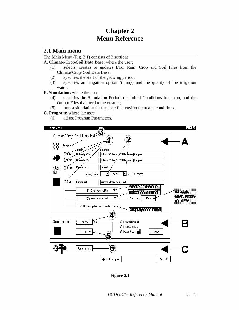
2.1 Main menu The Main Menu (Fig. 2.1) consists of 3 sections: A. Climate/Crop/Soil Data Base: where the user:
(1) selects, creates or updates ETo, Rain, Crop and Soil Files from the Climate/Crop/ Soil Data Base;
(2) specifies the start of the growing period; (3) specifies an irrigation option (if any) and the quality of the irrigation
water; B. Simulation: where the user:
(4) specifies the Simulation Period, the Initial Conditions for a run, and the Output Files that need to be created;
(5) runs a simulation for the specified environment and conditions. C. Program: where the user:
(6) adjust Program Parameters.
Figure 2.1

BUDGET – Reference Manual 2. 2
Main Menu
BUDGET – Reference Manual 2. 3
2.2 Climate input (ETo and Rain data) For each day of the simulation period, the program requires information concerning the weather conditions. Those conditions determine the amount of water that can infiltrate into the soil profile and that can be extracted from the soil profile by soil evaporation and crop transpiration. The climatic conditions are given by: - evaporative demand of the atmosphere for the given weather conditions. The
atmospheric demand is given by the evapotranspiration from the reference surface (ETo);
- rainfall depth, which is the amount of water collected in rain gauges installed on the field or at a nearby weather station.
The amount of water that is actually extracted from the soil profile or infiltrates into the soil profile can only be determined at run time by considering the infiltration rate of the top soil, crop characteristics (Kc) and soil water content in the top soil at that particular day. The data consist of daily, mean 10-day or mean monthly ETo and Rainfall observations. Simulations can run with climatic data of a specific year, mean average data not linked to a specific year, or even with ETo or Rainfall levels than are expected with a given probability (dependable ETo or Rainfall). At run time, the 10-day and monthly data are processed to derive daily ETo and Rain data (See Chapter 3, Processing of 10-day and monthly climatic data ). The climatic data can be - specified by the user at run time (this is the default setting, see 2.10 Run); - specified and saved in a file before running a simulation by selecting the Create
Command in the Main Menu, and by subsequently specifying the climatic data for a number of successive days, decades, or months. If the data consists of averages or dependable levels, the data is not linked to a specific year and its use is not restricted to simulations runs for a particular year;
- downloaded from an existing climate file by selecting the Select Command in the Main Menu. When selecting this Command, a list is displayed that contains all the files with extension ‘ETo’ (ETo data) or ‘PLU’ (rain data) in the specified directory. The user select the appropriate climatic file from this list;
- The user can import climate files in the data directory with for example the help of Windows Explorer. Climate files are text files with a specific data structure (Table 2.2) and with extension ‘ETo’ or ‘PLU’. The user can create its own climate files (use for example NOTEPAD) as long as the specific data structure is respected.
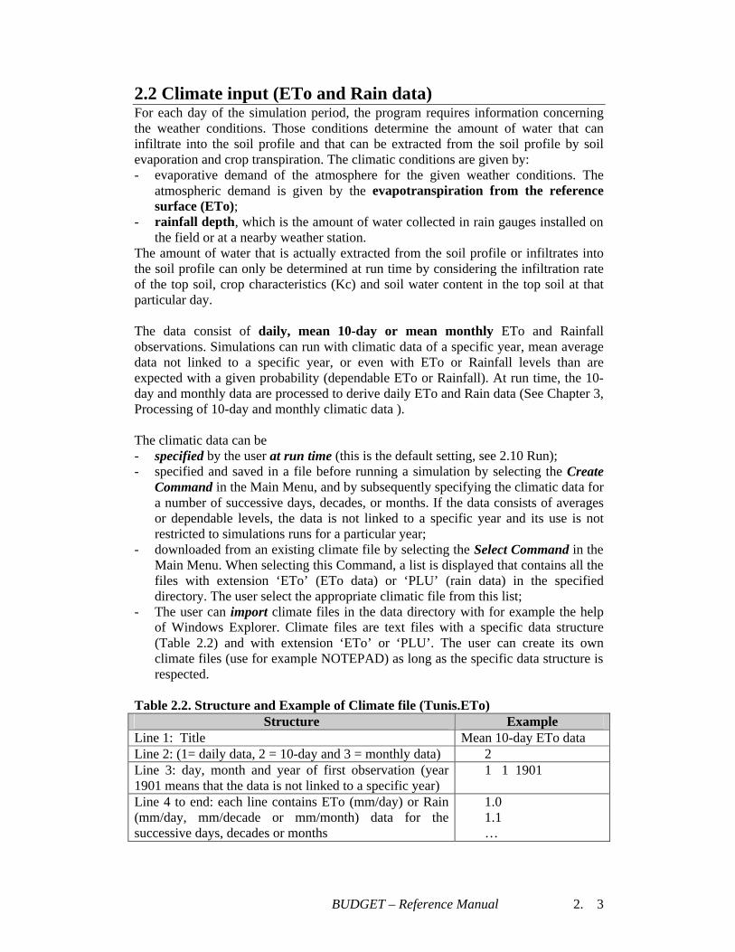
Table 2.2. Structure and Example of Climate file (Tunis.ETo)
Structure Example Line 1: Title Mean 10-day ETo data Line 2: (1= daily data, 2 = 10-day and 3 = monthly data) 2 Line 3: day, month and year of first observation (year 1901 means that the data is not linked to a specific year)
1 1 1901
Line 4 to end: each line contains ETo (mm/day) or Rain (mm/day, mm/decade or mm/month) data for the successive days, decades or months
1.0 1.1 …
BUDGET – Reference Manual 2. 4
2.3 Crop data 2.3.1 Select/Create crop file To specify the crop parameters, the user either - download the crop parameters from an existing file by selecting the Select
Command in the Main Menu. When selecting this Command, a list is displayed that contains all the files with extension ‘CRO’ in the specified directory (default path is the DATA subdirectory from BUDGET). The user selects the appropriate crop file from this list;
- create a new set of parameters that will be saved in a crop file by selecting the
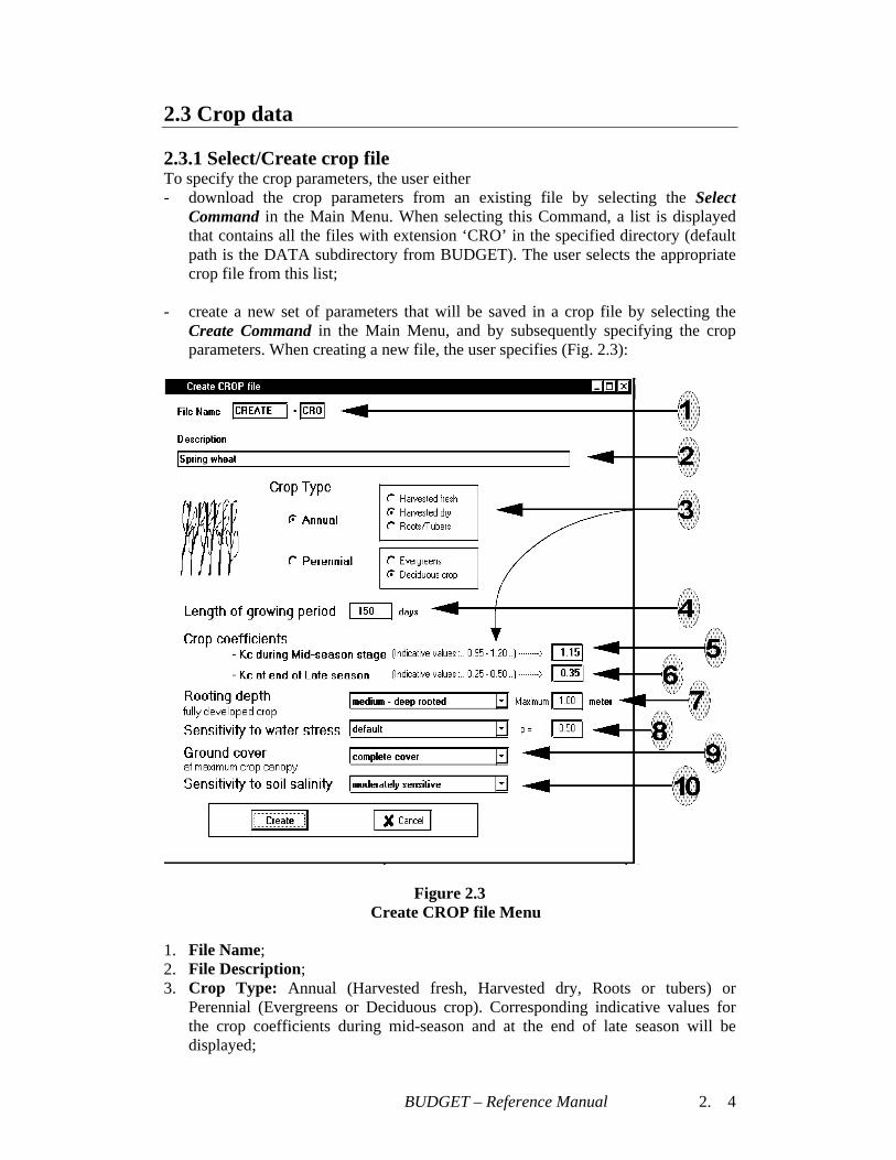
Create Command in the Main Menu, and by subsequently specifying the crop parameters. When creating a new file, the user specifies (Fig. 2.3):
Figure 2.3 Create CROP file Menu
1. File Name; 2. File Description; 3. Crop Type: Annual (Harvested fresh, Harvested dry, Roots or tubers) or
Perennial (Evergreens or Deciduous crop). Corresponding indicative values for the crop coefficients during mid-season and at the end of late season will be displayed;
BUDGET – Reference Manual 2. 5
4. Length of the growing period; 5. Crop coefficient during the mid-season stage. Indicative values for various
crops are given in Annex I, Table I.2; 6. Crop coefficient at the end of the late season stage. Indicative values for
various crops are given in Annex I, Table I.2; 7. Rooting depth for the fully developed crop: classes ranging from shallow
rooted crops to very deep-rooted crops. BUDGET generates the corresponding maximum effective rooting depth (Table 2.3a). The rooting depth can also be specified immediately. Indicative values for various crops are given in Annex I, Table I.3
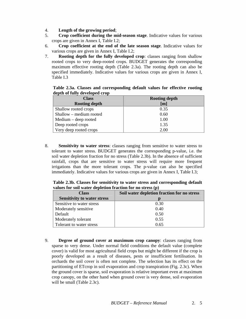
Table 2.3a. Classes and corresponding default values for effective rooting depth of fully developed crop
Class Rooting depth
Rooting depth [m]
Shallow rooted crops Shallow – medium rooted Medium – deep rooted Deep rooted crops Very deep rooted crops
0.35 0.60 1.00 1.35 2.00
8. Sensitivity to water stress: classes ranging from sensitive to water stress to
tolerant to water stress. BUDGET generates the corresponding p-value, i.e. the soil water depletion fraction for no stress (Table 2.3b). In the absence of sufficient rainfall, crops that are sensitive to water stress will require more frequent irrigations than the more tolerant crops. The p-value can also be specified immediately. Indicative values for various crops are given in Annex I, Table I.3;
Table 2.3b. Classes for sensitivity to water stress and corresponding default values for soil water depletion fraction for no stress (p)
Class Sensitivity to water stress
Soil water depletion fraction for no stress p
Sensitive to water stress Moderately sensitive Default Moderately tolerant Tolerant to water stress
0.30 0.40 0.50 0.55 0.65
9. Degree of ground cover at maximum crop canopy: classes ranging from
sparse to very dense. Under normal field conditions the default value (complete cover) is valid for most agricultural field crops but might be different if the crop is poorly developed as a result of diseases, pests or insufficient fertilisation. In orchards the soil cover is often not complete. The selection has its effect on the partitioning of ETcrop in soil evaporation and crop transpiration (Fig. 2.3c). When the ground cover is sparse, soil evaporation is relative important even at maximum crop canopy, on the other hand when ground cover is very dense, soil evaporation will be small (Table 2.3c).
BUDGET – Reference Manual 2. 6
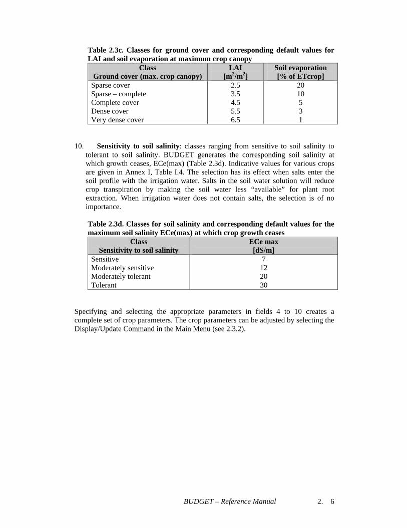
Table 2.3c. Classes for ground cover and corresponding default values for LAI and soil evaporation at maximum crop canopy
Class Ground cover (max. crop canopy)
LAI [m2/m2]
Soil evaporation [% of ETcrop]
Sparse cover Sparse – complete Complete cover Dense cover Very dense cover
2.5 3.5 4.5 5.5 6.5
20 10 5 3 1
10. Sensitivity to soil salinity: classes ranging from sensitive to soil salinity to
tolerant to soil salinity. BUDGET generates the corresponding soil salinity at which growth ceases, ECe(max) (Table 2.3d). Indicative values for various crops are given in Annex I, Table I.4. The selection has its effect when salts enter the soil profile with the irrigation water. Salts in the soil water solution will reduce crop transpiration by making the soil water less “available” for plant root extraction. When irrigation water does not contain salts, the selection is of no importance.
Table 2.3d. Classes for soil salinity and corresponding default values for the maximum soil salinity ECe(max) at which crop growth ceases
Class Sensitivity to soil salinity
ECe max [dS/m]
Sensitive Moderately sensitive Moderately tolerant Tolerant
7 12 20 30
Specifying and selecting the appropriate parameters in fields 4 to 10 creates a complete set of crop parameters. The crop parameters can be adjusted by selecting the Display/Update Command in the Main Menu (see 2.3.2).
BUDGET – Reference Manual 2. 7
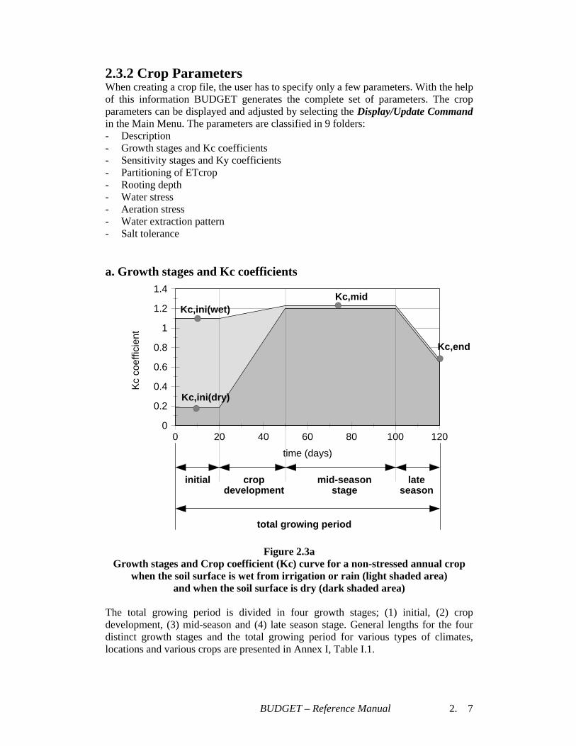
2.3.2 Crop Parameters When creating a crop file, the user has to specify only a few parameters. With the help of this information BUDGET generates the complete set of parameters. The crop parameters can be displayed and adjusted by selecting the Display/Update Command in the Main Menu. The parameters are classified in 9 folders: - Description - Growth stages and Kc coefficients - Sensitivity stages and Ky coefficients - Partitioning of ETcrop - Rooting depth - Water stress - Aeration stress - Water extraction pattern - Salt tolerance a. Growth stages and Kc coefficients
0 20 40 60 80 100 120
time (days)
0
0.2
0.4
0.6
0.8
1
1.2
1.4
Kc
coef
ficie
nt
initial cropdevelopment
mid-seasonstage
lateseason
total growing period
Kc,end
Kc,mid
Kc,ini(dry)
Kc,ini(wet)
Figure 2.3a Growth stages and Crop coefficient (Kc) curve for a non-stressed annual crop
when the soil surface is wet from irrigation or rain (light shaded area) and when the soil surface is dry (dark shaded area)
The total growing period is divided in four growth stages; (1) initial, (2) crop development, (3) mid-season and (4) late season stage. General lengths for the four distinct growth stages and the total growing period for various types of climates, locations and various crops are presented in Annex I, Table I.1.
BUDGET – Reference Manual 2. 8
Kc coefficients for various non-stressed, well-managed crops in subhumid climates are presented in Table I.2 of Annex I. As soil evaporation is an integrated part of crop evapotranspiration, the Kc coefficient is affected by wetting frequency and soil cover. BUDGET derives the crop coefficient curve (Fig. 2.3a) for a wet and dry soil surface from information on crop cover (see c Partitioning of ETcrop), the Kc value for a wet bare soil (see 2.9 Program Parameters) and Kc values specified by the user (Table 2.3a and 2.3a(bis)). Table 2.3a Crop coefficients for annual crop types Annual crop types Initial stage Kc,ini (dry) *1 ßà Kc,ini (wet) *2 Crop development stage …….. à Kc,mid
Mid-season stage Kc,mid ß specify
Late season stage Kc,mid à Kc,end ß specify *1 Kc Value determined by ground cover (LAI) at initial stage (see c Partitioning of ETcrop) *2 Kc value for a wet bare soil (see 2.9 Program Parameters) Table 2.3a(bis) Crop coefficients for perennial crop types Perennial crop types Initial stage Kc,ini(wet, shaded) *1 ß specify
Crop development stage …….. à Kc,mid
Mid-season stage Kc,mid ß specify
Late season stage Kc,mid à Kc,end ß specify *1 Kc value for a wet soil shaded by the perennial crop b. Sensitivity stages and Ky coefficients The yield response to water deficit for various sensitivity stages can be specified in this folder. The data will be used to convert water stress in estimates of yield depression (see Chapter 3, Estimation of Relative Yield). The user specifies for each stage its length and the corresponding yield response factor Ky. The higher the Ky value the more sensitive the crop will be to water deficit. In general, crops are more sensitive to water deficit during emergence, flowering and early yield formation than they are during the vegetative growth period and ripening (Doorenbos and Kassam, 1979). Values for yield response factor for various crops and sensitivity stages are presented in Annex I, Table I.5. If data is not available, the default value of 1 will be used for Ky for each of the stages. Consequently the decrease in yield will be directly proportionally with the water deficit throughout the growing season.
BUDGET – Reference Manual 2. 9
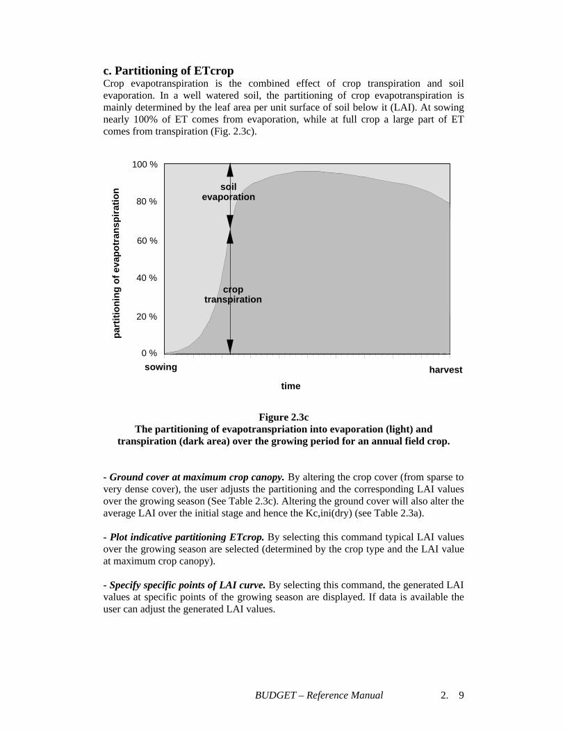
c. Partitioning of ETcrop Crop evapotranspiration is the combined effect of crop transpiration and soil evaporation. In a well watered soil, the partitioning of crop evapotranspiration is mainly determined by the leaf area per unit surface of soil below it (LAI). At sowing nearly 100% of ET comes from evaporation, while at full crop a large part of ET comes from transpiration (Fig. 2.3c).
100 %
par
titi
on
ing
of
evap
otr
ansp
irat
ion
sowing harvest
time
0 %
80 %
60 %
40 %
20 %
croptranspiration
soilevaporation
Figure 2.3c The partitioning of evapotranspriation into evaporation (light) and
transpiration (dark area) over the growing period for an annual field crop. - Ground cover at maximum crop canopy. By altering the crop cover (from sparse to very dense cover), the user adjusts the partitioning and the corresponding LAI values over the growing season (See Table 2.3c). Altering the ground cover will also alter the average LAI over the initial stage and hence the Kc,ini(dry) (see Table 2.3a). - Plot indicative partitioning ETcrop. By selecting this command typical LAI values over the growing season are selected (determined by the crop type and the LAI value at maximum crop canopy). - Specify specific points of LAI curve. By selecting this command, the generated LAI values at specific points of the growing season are displayed. If data is available the user can adjust the generated LAI values.
BUDGET – Reference Manual 2. 10
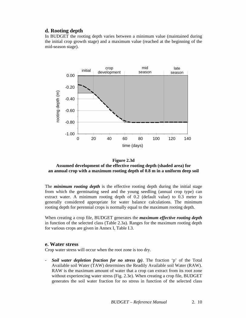
d. Rooting depth In BUDGET the rooting depth varies between a minimum value (maintained during the initial crop growth stage) and a maximum value (reached at the beginning of the mid-season stage).
0 20 40 60 80 100 120 140
time (days)
0.00
-0.20
-0.40
-0.60
-0.80
-1.00
root
ing
dept
h (m
)
initialcrop
developmentmid
seasonlate
season
Figure 2.3d
Assumed development of the effective rooting depth (shaded area) for an annual crop with a maximum rooting depth of 0.8 m in a uniform deep soil
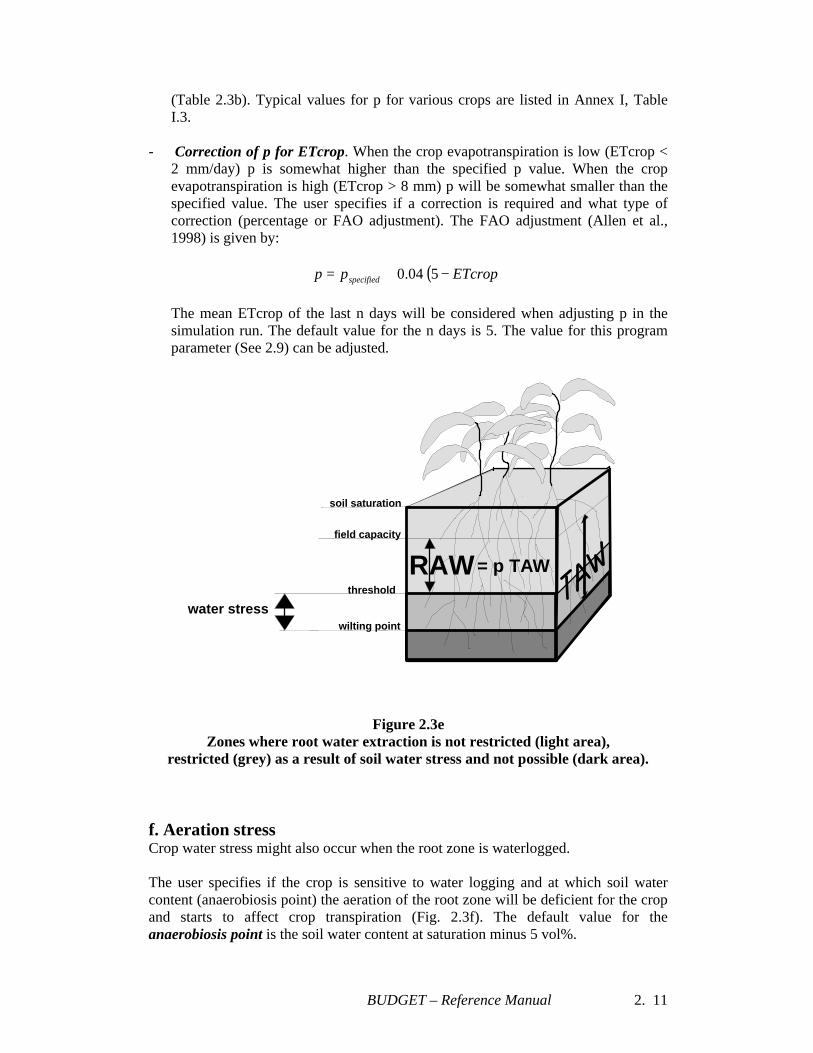
The minimum rooting depth is the effective rooting depth during the initial stage from which the germinating seed and the young seedling (annual crop type) can extract water. A minimum rooting depth of 0.2 (default value) to 0.3 meter is generally considered appropriate for water balance calculations. The minimum rooting depth for perennial crops is normally equal to the maximum rooting depth. When creating a crop file, BUDGET generates the maximum effective rooting depth in function of the selected class (Table 2.3a). Ranges for the maximum rooting depth for various crops are given in Annex I, Table I.3. e. Water stress Crop water stress will occur when the root zone is too dry. - Soil water depletion fraction for no stress (p). The fraction ‘p’ of the Total
Available soil Water (TAW) determines the Readily Available soil Water (RAW). RAW is the maximum amount of water that a crop can extract from its root zone without experiencing water stress (Fig. 2.3e). When creating a crop file, BUDGET generates the soil water fraction for no stress in function of the selected class
BUDGET – Reference Manual 2. 11
(Table 2.3b). Typical values for p for various crops are listed in Annex I, Table I.3.
- Correction of p for ETcrop. When the crop evapotranspiration is low (ETcrop <
2 mm/day) p is somewhat higher than the specified p value. When the crop evapotranspiration is high (ETcrop > 8 mm) p will be somewhat smaller than the specified value. The user specifies if a correction is required and what type of correction (percentage or FAO adjustment). The FAO adjustment (Allen et al., 1998) is given by:
( )ETcroppp specified −+= 504.0
The mean ETcrop of the last n days will be considered when adjusting p in the simulation run. The default value for the n days is 5. The value for this program parameter (See 2.9) can be adjusted.
field capacity
threshold
wilting point
soil saturation
water stress
= p TAWRAW
Figure 2.3e
Zones where root water extraction is not restricted (light area), restricted (grey) as a result of soil water stress and not possible (dark area).
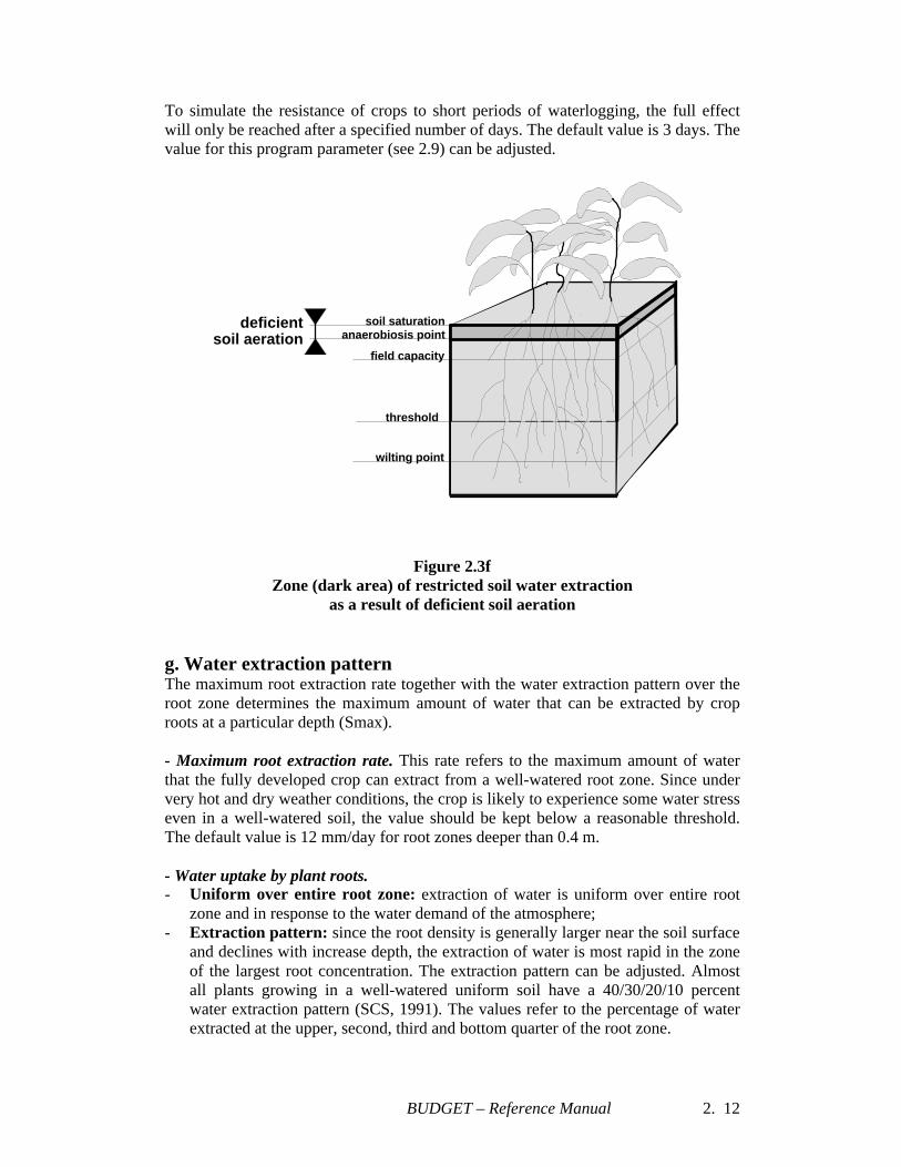
f. Aeration stress Crop water stress might also occur when the root zone is waterlogged. The user specifies if the crop is sensitive to water logging and at which soil water content (anaerobiosis point) the aeration of the root zone will be deficient for the crop and starts to affect crop transpiration (Fig. 2.3f). The default value for the anaerobiosis point is the soil water content at saturation minus 5 vol%.
BUDGET – Reference Manual 2. 12
To simulate the resistance of crops to short periods of waterlogging, the full effect will only be reached after a specified number of days. The default value is 3 days. The value for this program parameter (see 2.9) can be adjusted.
field capacity
threshold
wilting point
soil saturationanaerobiosis point
deficientsoil aeration
Figure 2.3f
Zone (dark area) of restricted soil water extraction as a result of deficient soil aeration
g. Water extraction pattern The maximum root extraction rate together with the water extraction pattern over the root zone determines the maximum amount of water that can be extracted by crop roots at a particular depth (Smax). - Maximum root extraction rate. This rate refers to the maximum amount of water that the fully developed crop can extract from a well-watered root zone. Since under very hot and dry weather conditions, the crop is likely to experience some water stress even in a well-watered soil, the value should be kept below a reasonable threshold. The default value is 12 mm/day for root zones deeper than 0.4 m. - Water uptake by plant roots. - Uniform over entire root zone: extraction of water is uniform over entire root
zone and in response to the water demand of the atmosphere; - Extraction pattern: since the root density is generally larger near the soil surface
and declines with increase depth, the extraction of water is most rapid in the zone of the largest root concentration. The extraction pattern can be adjusted. Almost all plants growing in a well-watered uniform soil have a 40/30/20/10 percent water extraction pattern (SCS, 1991). The values refer to the percentage of water extracted at the upper, second, third and bottom quarter of the root zone.
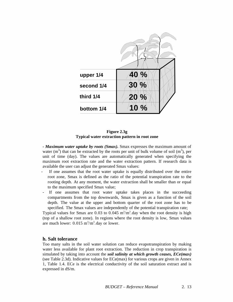
BUDGET – Reference Manual 2. 13
40 %30 %
20 %10 %
upper 1/4
second 1/4
third 1/4
bottom 1/4
Figure 2.3g
Typical water extraction pattern in root zone
- Maximum water uptake by roots (Smax). Smax expresses the maximum amount of water (m3) that can be extracted by the roots per unit of bulk volume of soil (m3), per unit of time (day). The values are automatically generated when specifying the maximum root extraction rate and the water extraction pattern. If research data is available the user can adjust the generated Smax values:
- If one assumes that the root water uptake is equally distributed over the entire root zone, Smax is defined as the ratio of the potential transpiration rate to the rooting depth. At any moment, the water extraction shall be smaller than or equal to the maximum specified Smax value;
- If one assumes that root water uptake takes places in the succeeding compartments from the top downwards, Smax is given as a function of the soil depth. The value at the upper and bottom quarter of the root zone has to be specified. The Smax values are independently of the potential transpiration rate;
Typical values for Smax are 0.03 to 0.045 m3/m3.day when the root density is high (top of a shallow root zone). In regions where the root density is low, Smax values are much lower: 0.015 m3/m3.day or lower. h. Salt tolerance Too many salts in the soil water solution can reduce evapotranspiration by making water less available for plant root extraction. The reduction in crop transpiration is simulated by taking into account the soil salinity at which growth ceases, ECe(max) (see Table 2.3d). Indicative values for ECe(max) for various crops are given in Annex 1, Table 1.4. ECe is the electrical conductivity of the soil saturation extract and is expressed in dS/m.
BUDGET – Reference Manual 2. 13
2.4 Profile description 2.4.1 Select/Create soil file To specify the soil parameters, the user either: - download the soil parameters from an existing file by selecting the Select
Command in the Main Menu. When selecting this Command, a list is displayed that contains all the files with extension ‘SOL’ in the specified directory (default path is the DATA subdirectory from BUDGET). The user selects the appropriate crop file from this list;
- create a new set of parameters that will be saved in a soil file by selecting the
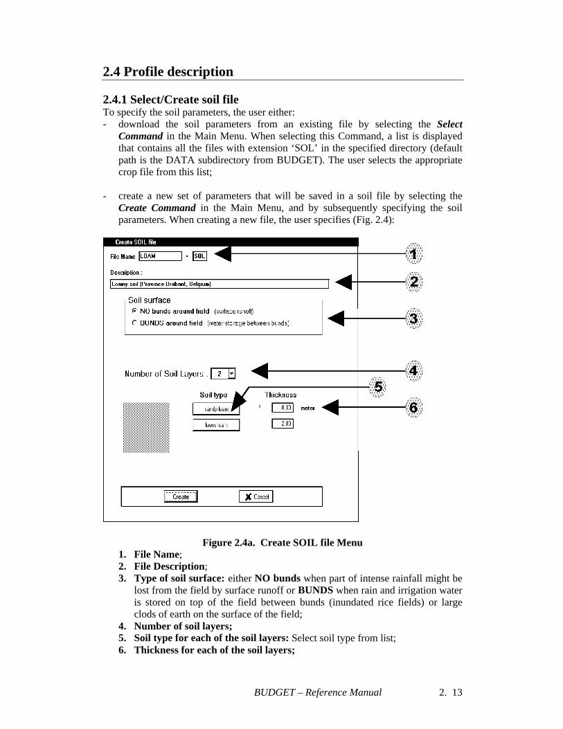
Create Command in the Main Menu, and by subsequently specifying the soil parameters. When creating a new file, the user specifies (Fig. 2.4):
Figure 2.4a. Create SOIL file Menu
1. File Name; 2. File Description; 3. Type of soil surface: either NO bunds when part of intense rainfall might be
lost from the field by surface runoff or BUNDS when rain and irrigation water is stored on top of the field between bunds (inundated rice fields) or large clods of earth on the surface of the field;
4. Number of soil layers; 5. Soil type for each of the soil layers: Select soil type from list; 6. Thickness for each of the soil layers;
BUDGET – Reference Manual 2. 14
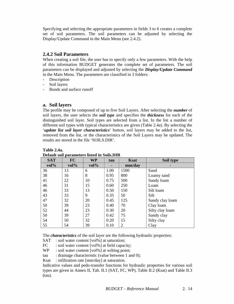
Specifying and selecting the appropriate parameters in fields 3 to 6 creates a complete set of soil parameters. The soil parameters can be adjusted by selecting the Display/Update Command in the Main Menu (see 2.4.2). 2.4.2 Soil Parameters When creating a soil file, the user has to specify only a few parameters. With the help of this information BUDGET generates the complete set of parameters. The soil parameters can be displayed and adjusted by selecting the Display/Update Command in the Main Menu. The parameters are classified in 3 folders: - Description - Soil layers - Bunds and surface runoff a. Soil layers The profile may be composed of up to five Soil Layers. After selecting the number of soil layers, the user selects the soil type and specifies the thickness for each of the distinguished soil layer. Soil types are selected from a list. In the list a number of different soil types with typical characteristics are given (Table 2.4a). By selecting the ‘update list soil layer characteristics’ button, soil layers may be added to the list, removed from the list, or the characteristics of the Soil Layers may be updated. The results are stored in the file ‘SOILS.DIR’. Table 2.4a. Default soil parameters listed in Soils.DIR
SAT FC WP tau Ksat Soil type vol% vol% vol% - mm/day -
36 38 41 46 46 43 47 50 52 50 54 55
13 16 22 31 33 33 32 39 44 39 50 54
6 8 10 15 13 9 20 23 23 27 32 39
1.00 0.95 0.75 0.60 0.50 0.35 0.45 0.40 0.30 0.42 0.20 0.10
1500 800 500 250 150 50 125 70 20 75 15 2
Sand Loamy sand Sandy loam Loam Silt loam Silt Sandy clay loam Clay loam Silty clay loam Sandy clay Silty clay Clay
The characteristics of the soil layer are the following hydraulic properties: SAT : soil water content [vol%] at saturation; FC : soil water content [vol%] at field capacity; WP : soil water content [vol%] at wilting point; tau : drainage characteristic (value between 1 and 0); Ksat : infiltration rate [mm/day] at saturation. Indicative values and pedo-transfer functions for hydraulic properties for various soil types are given in Annex II, Tab. II.1 (SAT, FC, WP), Table II.2 (Ksat) and Table II.3 (tau).
BUDGET – Reference Manual 2. 15
The difference in water content at Field Capacity and Wilting Point determines the total amount of water (TAW) that is available for crop transpiration. Ksat determines the maximum rate with which water can infiltrate in the soil. Its value determines also the default CN value (see Table 2.4b). The amount of water that drains out of a soil layer (when the soil water content is above field capacity) is fully determined by the drainage characteristic, tau. The drainage characteristic is strongly correlated with Ksat (see Annex II) Table 2.4b Infiltration rate of top soil layer and corresponding CN default value
Infiltration rate [mm/day]
CN default value
> 250 250 – 50 50 – 10
< 10
65 75 80 85
b. Bunds and surface runoff When bunds are present, the user specifies the height of the bunds. In the absence of bunds, part of intense rainfall might be lost by surface runoff. The amount of rainfall lost by surface runoff is based on the Curve Number method of the US Soil Conservation Service (see Chapter 3). The displayed default value for CN is based on the infiltration rate of the top layer (Table 2.4b). The default and specified CN value refer to the value for antecedent moisture class II (AMC II). If requested, BUDGET adjusts the CN value to the relative wetness of the topsoil during the simulation run. As such the estimate of surface runoff takes the variable storage capacity of the soil into account, which will be different when the topsoil is wet (AMC III) or dry (AMC I). The thickness of the topsoil that will be considered for the determination of its soil water content and corresponding adjustment of CN is a Program Parameter that can be altered (see 2.9 Program parameters). By selecting ‘No adjustment’ the CN value is not corrected in function of AMC. For more information see Chapter 3 (3.3 Runoff subroutine).
BUDGET – Reference Manual 2. 16
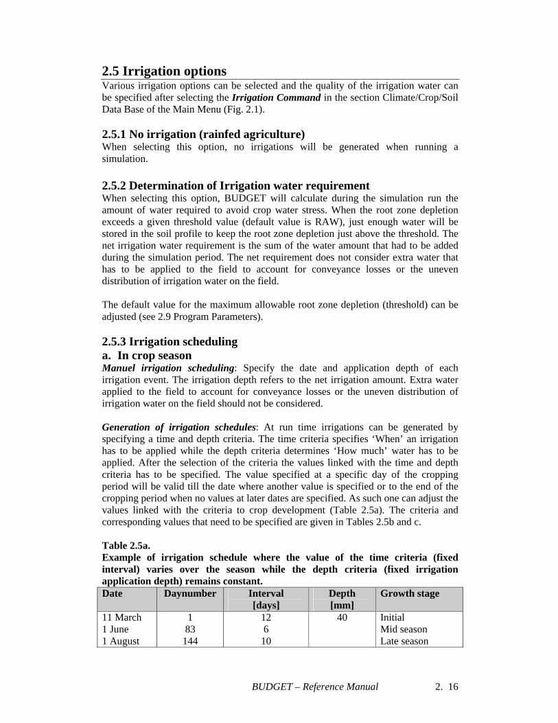
2.5 Irrigation options Various irrigation options can be selected and the quality of the irrigation water can be specified after selecting the Irrigation Command in the section Climate/Crop/Soil Data Base of the Main Menu (Fig. 2.1). 2.5.1 No irrigation (rainfed agriculture) When selecting this option, no irrigations will be generated when running a simulation. 2.5.2 Determination of Irrigation water requirement When selecting this option, BUDGET will calculate during the simulation run the amount of water required to avoid crop water stress. When the root zone depletion exceeds a given threshold value (default value is RAW), just enough water will be stored in the soil profile to keep the root zone depletion just above the threshold. The net irrigation water requirement is the sum of the water amount that had to be added during the simulation period. The net requirement does not consider extra water that has to be applied to the field to account for conveyance losses or the uneven distribution of irrigation water on the field. The default value for the maximum allowable root zone depletion (threshold) can be adjusted (see 2.9 Program Parameters). 2.5.3 Irrigation scheduling a. In crop season Manuel irrigation scheduling: Specify the date and application depth of each irrigation event. The irrigation depth refers to the net irrigation amount. Extra water applied to the field to account for conveyance losses or the uneven distribution of irrigation water on the field should not be considered. Generation of irrigation schedules: At run time irrigations can be generated by specifying a time and depth criteria. The time criteria specifies ‘When’ an irrigation has to be applied while the depth criteria determines ‘How much’ water has to be applied. After the selection of the criteria the values linked with the time and depth criteria has to be specified. The value specified at a specific day of the cropping period will be valid till the date where another value is specified or to the end of the cropping period when no values at later dates are specified. As such one can adjust the values linked with the criteria to crop development (Table 2.5a). The criteria and corresponding values that need to be specified are given in Tables 2.5b and c. Table 2.5a. Example of irrigation schedule where the value of the time criteria (fixed interval) varies over the season while the depth criteria (fixed irrigation application depth) remains constant. Date Daynumber Interval
[days] Depth [mm]
Growth stage
11 March 1 June 1 August
1 83
144
12 6
10
40 Initial Mid season Late season

BUDGET – Reference Manual 2. 17
Table 2.5b. Time criteria and corresponding parameter to be specified Criteria Specify Fixed interval Interval between irrigations (for example 10 days) Allowable depletion amount Amount of water that can be depleted from the root
zone (counting from field capacity) before an irrigation has to be applied (for example 30 mm)
Allowable fraction of Readily Available soil Water (RAW)
Percentage of RAW that can be depleted before an irrigation has to be applied (for example 100 %)
Table 2.5c. Depth criteria and corresponding parameter to be specified Criteria Specify Back to field capacity Additional water depth. The applied irrigation water
will set the soil water content in the root zone exactly to field capacity if 0 (mm) is specified. It is possible to plan an over- or under-irrigation by indicating the extra amount that has to be applied on top of the water required to bring the root zone back to field capacity (for example + 20 mm) or the shortage (for example – 10 mm)
Fixed application depth Net irrigation application depth b. Out of crop season When the simulation period is not fully linked with the cropping period (see 2.6 Simulation Period), irrigation events can also be scheduled before and after the cropping period. This allows the users to simulate a pre-irrigation before the sowing or planting of the crop or to schedule irrigations out of the crop season to leach accumulated salts out of the root zone. c. Irrigation water quality The irrigation water quality (Tab. 2.5d) refers to the salt content of the water. It is expressed on the basis of its electrical conductivity (ECw). Table 2.5d Classification of irrigation water (Ayers and Westcot, 1985)
ECw in [dS/m] Degree of restriction in use < 0.7
0.7 – 3.0 > 3.0
None slight to moderate severe
BUDGET – Reference Manual 2. 18
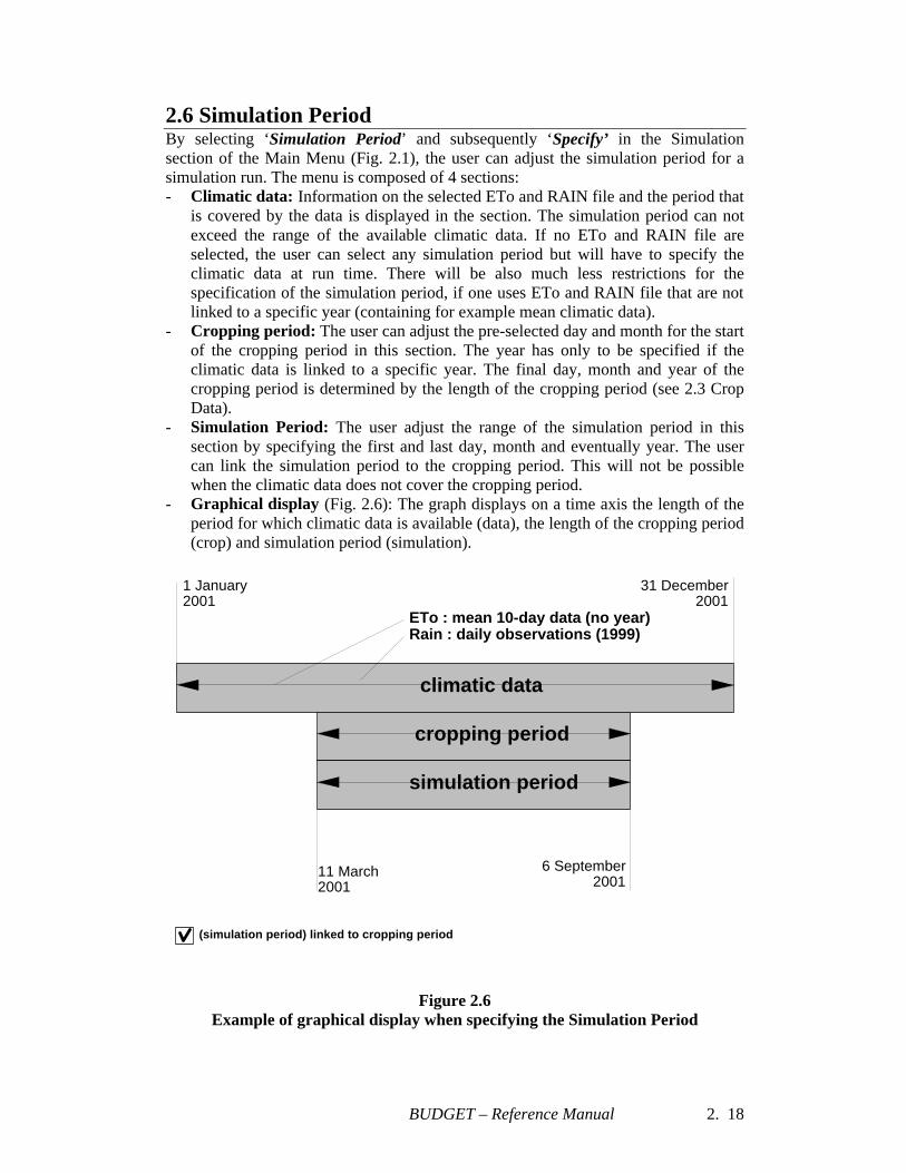
2.6 Simulation Period By selecting ‘Simulation Period’ and subsequently ‘Specify’ in the Simulation section of the Main Menu (Fig. 2.1), the user can adjust the simulation period for a simulation run. The menu is composed of 4 sections: - Climatic data: Information on the selected ETo and RAIN file and the period that
is covered by the data is displayed in the section. The simulation period can not exceed the range of the available climatic data. If no ETo and RAIN file are selected, the user can select any simulation period but will have to specify the climatic data at run time. There will be also much less restrictions for the specification of the simulation period, if one uses ETo and RAIN file that are not linked to a specific year (containing for example mean climatic data).
- Cropping period: The user can adjust the pre-selected day and month for the start of the cropping period in this section. The year has only to be specified if the climatic data is linked to a specific year. The final day, month and year of the cropping period is determined by the length of the cropping period (see 2.3 Crop Data).
- Simulation Period: The user adjust the range of the simulation period in this section by specifying the first and last day, month and eventually year. The user can link the simulation period to the cropping period. This will not be possible when the climatic data does not cover the cropping period.
- Graphical display (Fig. 2.6): The graph displays on a time axis the length of the period for which climatic data is available (data), the length of the cropping period (crop) and simulation period (simulation).
1 January2001
31 December2001
11 March2001
6 September2001
climatic data
cropping period
simulation period
ETo : mean 10-day data (no year)Rain : daily observations (1999)
(simulation period) linked to cropping period
Figure 2.6 Example of graphical display when specifying the Simulation Period
BUDGET – Reference Manual 2. 19
2.7 Initial conditions By selecting ‘Initial conditions’ and subsequently ‘Specify’ in the Simulation section of the Main Menu (Fig. 2.1), the user can adjust the initial conditions for a simulation run. 2.7.1 Initial soil water and salt conditions Initial soil water content and salt contents can be adjusted: - the initial soil water content of the total profile may be set at Saturation, Field
Capacity, Wilting Point or may be specified individually for each of the soil compartments;
- the initial salt content of the total profile may be set at a specific value or may be specified individually for each of the soil compartments. The ECe is defined as the electrical conductivity of the soil water solution after the addition of a sufficient quantity of distilled water to bring the soil water content to saturation.
The initial conditions in the soil profile are strongly determined by the climatic conditions (ETo and Rain) and irrigation applications in the period before the simulation period. If the simulation period starts at the end of a very rainy season, the soil water content of the soil profile might be close to field capacity. If the simulation starts in the hot dry season, the topsoil might be wet by pre-irrigation but the subsoil will be dry and the water content close to wilting point. If the field is surrounded by bunds the user can additionally adjust: - the water depth on top of the soil surface between the bunds; - the salinity (Electrical Conductivity) of the water stored on the soil surface. 2.7.2 Soil cover outside growing period If the simulation period is not fully linked with the cropping period (see 2.6 Simulation Period), the user can specify the soil cover (mulch) of the fallow land before and/or after the cropping period. 2.7.3 Cumulative counters Cumulative counters keep track of the sum of the daily values of parameters of the soil water balance and of the expected relative yield. These counters are, by default, automatically reset at zero (the expected relative yield at 100 %) at the beginning of each simulation run. If the default option is not selected (see 2.9 Program Parameters) the value of the cumulative counters and expected yield are kept for the next run. In the menu ‘Cumulative counters’, the user can reset the counters at any time to their initial value.

BUDGET – Reference Manual 2. 20
2.8 Output files By selecting ‘Output Files’ and subsequently ‘Specify’ in the section Simulation of the Main Menu (Fig. 2.1), the user can switch the creation of 8 output files individually ON or OFF. The files (see Annex III) contain daily information of: - the water content of each soil compartment (file COMP.OUT); - the water content of each soil layer (file LAYER.OUT); - the value of the different terms of the water balance (file WABAL.OUT); - the fluxes between compartments (file FLUXES.OUT); - the salt content of each soil compartment (file SALT.OUT); - the value of the different terms of the salt balance (file SALTBAL.OUT); - the root zone depletion at the beginning and end of the day (file DEPL.OUT); - the net irrigation requirement (file INET.OUT). BUDGET overwrites previous recorded data, each time a simulation run is started (by pushing on the ‘Run’ button in the Main Menu). To avoid loss of data, the name as well as the path of output files can be modified. The contents of the Output Files can be displayed at the end of the simulation run by selecting ‘Display’ in the Simulation section of the Main Menu. The data can be aggregated in 10-day, monthly or yearly intervals.
BUDGET – Reference Manual 2. 21
2.9 Program parameters When starting BUDGET, default values for program parameters are extracted from the ‘Default.PAR’ file in the BUDGET main directory. The default values are either selected from literature or are the results of sensitivity analysis. By selecting ‘Parameters’ at the bottom of the Main Menu (Fig. 2.1), the user can adjust the default values. The adjustments are only valid during the session. (To fix values of program parameters to other default values, the user has to modify the values in the ‘Default.PAR’ file). The program parameters are classified in 9 folders: - Display - Evaporation - Transpiration - Salinity - Surface runoff - Soil compartments - Initial Conditions - Irrigation - Effective Rainfall 2.9.1 Display During the simulation run, the program will plot the value of one particular parameter. The user selects in this menu the specific parameter as well as its maximum value. 2.9.2 Evaporation The user can adjust parameters, which affects the simulation of soil evaporation: - The two regression coefficients for the Ritchie-type equation; - The crop coefficient for a bare wet soil; - The depth of soil water extraction by evaporation See Chapter 3, Crop evapotranspiration for more information. 2.9.3 Transpiration The user can adjust parameters, which affects the simulation of crop transpiration: - The number of days over which crop evapotranspiration will be averaged for the
adjustment of the maximum depletion factor for no stress (p); - The number of days after which the deficient aeration conditions will have its full
effect. 2.9.4 Salinity The user can adjust parameters, which affects the simulation of salt movement in the soil profile: - The Response factor for global salt diffusion. The value for the global diffusion
factor specifies the swiftness with which equilibrium is reached between the salt content of the various cells;
- Salt solubility: The salt concentration at which salts will precipitate. The value depends on soil temperature, type of soil solution and type of salts.
See Chapter 3, Salt transport for more information.
BUDGET – Reference Manual 2. 22
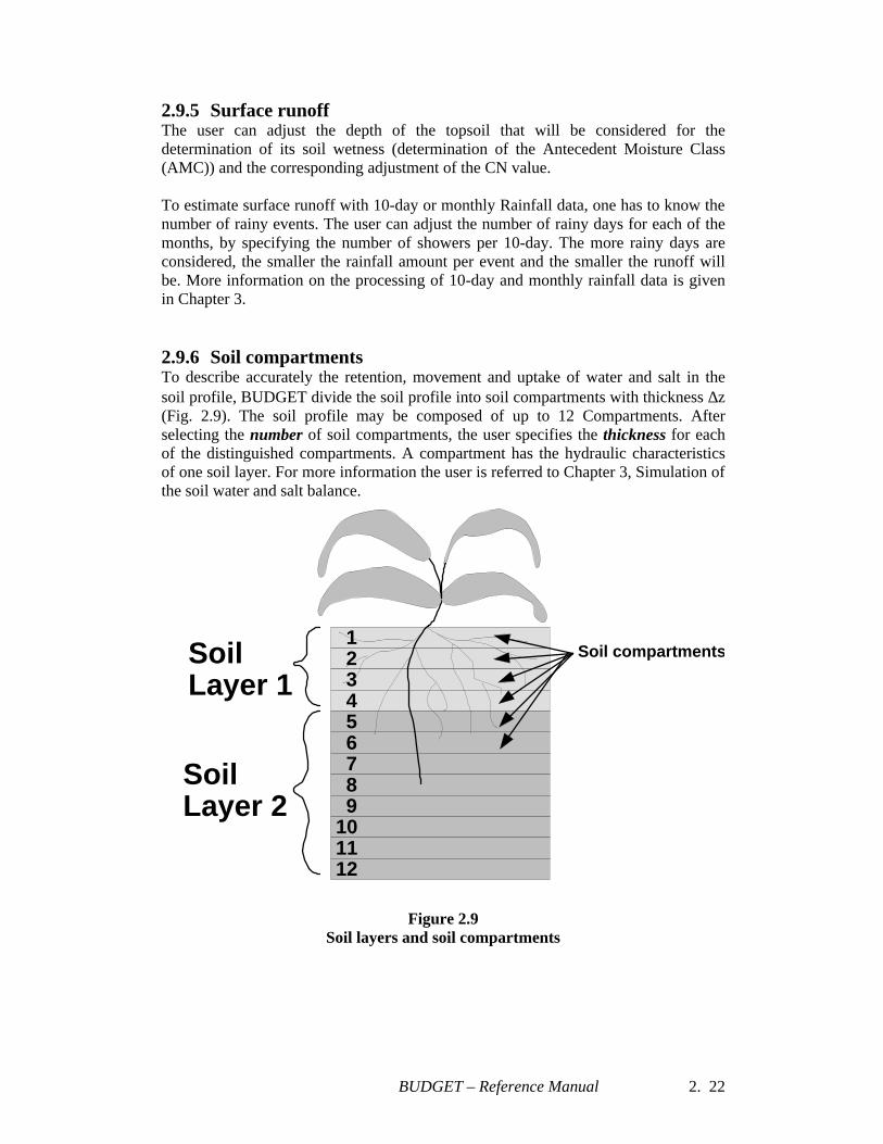
2.9.5 Surface runoff The user can adjust the depth of the topsoil that will be considered for the determination of its soil wetness (determination of the Antecedent Moisture Class (AMC)) and the corresponding adjustment of the CN value. To estimate surface runoff with 10-day or monthly Rainfall data, one has to know the number of rainy events. The user can adjust the number of rainy days for each of the months, by specifying the number of showers per 10-day. The more rainy days are considered, the smaller the rainfall amount per event and the smaller the runoff will be. More information on the processing of 10-day and monthly rainfall data is given in Chapter 3. 2.9.6 Soil compartments To describe accurately the retention, movement and uptake of water and salt in the soil profile, BUDGET divide the soil profile into soil compartments with thickness ∆z (Fig. 2.9). The soil profile may be composed of up to 12 Compartments. After selecting the number of soil compartments, the user specifies the thickness for each of the distinguished compartments. A compartment has the hydraulic characteristics of one soil layer. For more information the user is referred to Chapter 3, Simulation of the soil water and salt balance.
SoilLayer 1
SoilLayer 2
Soil compartments123
121110987654
Figure 2.9 Soil layers and soil compartments
BUDGET – Reference Manual 2. 23
2.9.7 Initial conditions When starting a new simulation run, the user can either Reset the soil water and salinity conditions in a soil profile to the specified initial conditions (see 2.7) or Keep the values of the previous runs. The selection depends on what one wants to simulate: - RESET: successive simulation runs are not linked in time or apply to different
fields; - KEEP: the various runs refer all to one particular field and are successive in time.
If in a field one crop after another is grown and the user wants to keep track of the soil water content and/or the building up of salts in the soil profile, the conditions at the end of a simulation run will be the initial conditions for the next run. It is obvious that in such cases the user can not change the soil type between two simulation runs.
2.9.8 Irrigation When calculating the net irrigation requirement, BUDGET keeps the root zone depletion above a threshold value. The user can vary this threshold from 0 (field capacity) to 100 percent (maximum allowable depletion to avoid water stress) of RAW. 2.9.9 Effective rainfall Effective rainfall is that part of rainfall that is not lost by surface run-off or deep percolation but is stored in the root zone. If the rainfall data consist of 10-day or monthly values, the rainfall distribution over the period is unknown and the amount of water lost by surface runoff and drainage can not be determined by solving the water balance equation. For such cases, BUDGET determines (after the subtraction of the estimated surface runoff (see e)) the amount of rainfall that will be stored in the root zone by one or another procedure. The ineffective part of the rainfall is assumed to have drained out of the root zone and is stored immediately below the root zone. The following procedures can be selected: - 100 percent effective: All rainfall is stored in the root zone; - USDA-SCS procedure: The amount of rainfall stored in the root zone depends on
the 10-day or monthly rainfall amount and the crop evapotranspiration rate during that period;
- Percentage of 10-day/Monthly rainfall: The percentage of the rainfall that is stored in the root zone is specified by the user.
More information on the processing of 10-day and monthly rainfall data is given in Chapter 3.
BUDGET – Reference Manual 2. 24
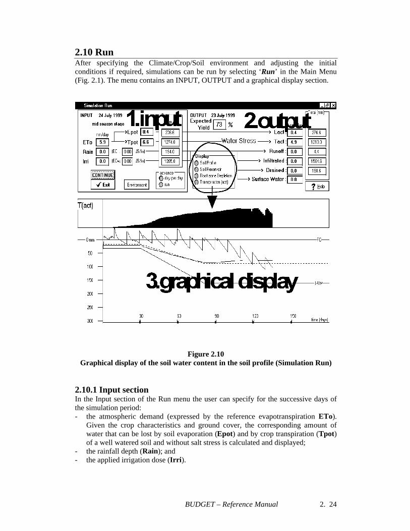
2.10 Run After specifying the Climate/Crop/Soil environment and adjusting the initial conditions if required, simulations can be run by selecting ‘Run’ in the Main Menu (Fig. 2.1). The menu contains an INPUT, OUTPUT and a graphical display section.
Figure 2.10 Graphical display of the soil water content in the soil profile (Simulation Run)
2.10.1 Input section In the Input section of the Run menu the user can specify for the successive days of the simulation period: - the atmospheric demand (expressed by the reference evapotranspiration ETo).
Given the crop characteristics and ground cover, the corresponding amount of water that can be lost by soil evaporation (Epot) and by crop transpiration (Tpot) of a well watered soil and without salt stress is calculated and displayed;
- the rainfall depth (Rain); and - the applied irrigation dose (Irri).
BUDGET – Reference Manual 2. 25
If climatic data is retrieved from ETo and RAIN files and if irrigations are generated by the program according to the selected option in the Main Menu, the user is unable to specify any data at run time. By clicking on the ‘Environment’ button, information on the selected Climate, Crop and Soil file, the irrigation option and on the cropping and simulation periods are displayed. By hitting the ‘START’ button, the simulation run starts and: - advance with a time step of one day (select ‘day per day’ as the ‘advance’ option).
With this option the user has to click each time on the ‘CONTINUE’ button to advance one day in the simulation period;
- runs through the simulation period (select ‘run’ as the ‘advance’ option). This option is only possible if climatic data is retrieved from files.
By hitting the ‘EXIT’ button the simulation is terminated and one returns to the Main Menu. 2.10.2 Output section At the start of each day of a simulation run, the output of the previous day is displayed. Information is given on the: - net irrigation requirement; - actual amount of water lost by soil evaporation (Eact); - actual amount of water lost by crop transpiration (Tact); - amount of water lost by surface runoff (Runoff); - amount of water that has been infiltrated in the soil profile (Infiltrated); - amount of water that drains out of the bottom compartment of the soil profile
(Drained); - amount of water that is stored between bunds on top of the soil surface (Surface
water); - expected relative yield at the end of the growing period (Expected Yield); and - information on the salt content of the soil water (ECe) at various depths in the soil
profile (visual display is soil profile). ECe is calculated by considering only the salts that can be dissolved in the soil saturation extract.
Cumulative counters keep track of the sum of Input and Output Parameters. 2.10.3 Graphical displays The user can select different visual displays: - cross section of the soil profile: The rooting depth, the salt and water content of
each soil compartment is displayed; - soil reservoir: The root zone is presented as a reservoir in which the soil water
content varies as a result of incoming and outgoing fluxes and of soil water extraction;
- root zone depletion: the root zone depletion, as well as RAW and TAW are plotted in function of time;
- parameter: During the simulation run, the program will plot the value of the selected parameter (see 2.9a for its selection).
BUDGET – Reference Manual 2. 26
Figure 2.10b Graphical displays
Cross section of soil profile
Soil reservoir
Root zone depletion
BUDGET – Reference Manual 3. 27
Chapter 3 Calculation procedures
3.1 Simulation of the soil water and salt balance In a simplified model, the root zone is considered as one single reservoir (Fig. 3.1a). By keeping track of the incoming and outgoing water and salt fluxes at the boundaries of the root zone, the amount of water and salt retained in the root zone can be calculated at any moment of the season by means of a soil water balance.
runoff
irrigationrainfall
capillaryrise
deeppercolation
sto
red
so
il w
ater
(m
m)
field capacity
wilting point
croptranspiration
0.0
soilevaporation
Figure 3.1a The root zone as a reservoir
Water is added to the soil by rainfall and irrigation. Salts enter the soil profile as solutes with the irrigation water. When the rainfall intensity is too high, part of the precipitation might be lost by surface runoff and only a fraction will infiltrate. The infiltrated water can not always be retained in the root zone. When the root zone is too wet, part of the soil water solution (salts and water) percolates out of the root zone. Water and salt can also be transported to the root zone by capillary rise from a shallow groundwater table. Processes such as soil evaporation and crop transpiration remove water from the reservoir. To describe accurately the retention, movement and uptake of water and salt in the soil profile throughout the growing season, simulation models commonly divide both
BUDGET – Reference Manual 3. 28
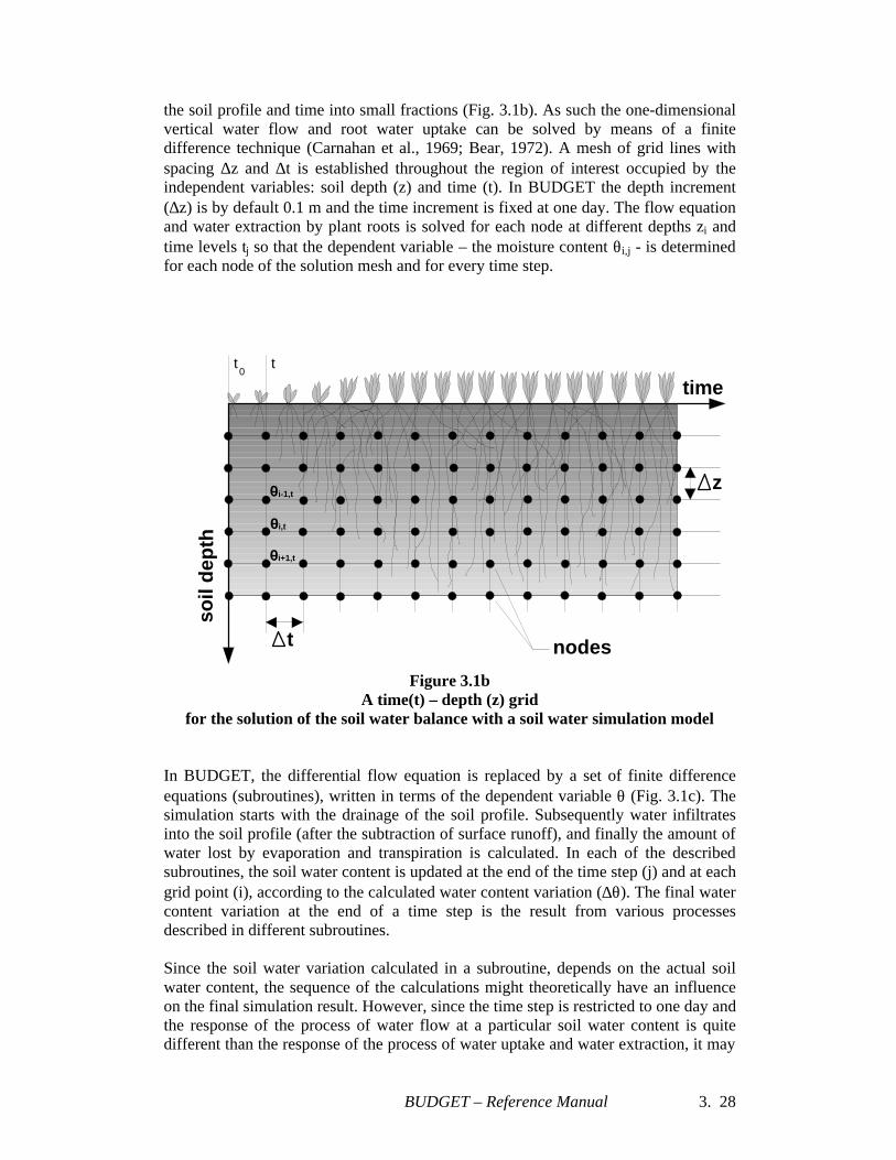
the soil profile and time into small fractions (Fig. 3.1b). As such the one-dimensional vertical water flow and root water uptake can be solved by means of a finite difference technique (Carnahan et al., 1969; Bear, 1972). A mesh of grid lines with spacing ∆z and ∆t is established throughout the region of interest occupied by the independent variables: soil depth (z) and time (t). In BUDGET the depth increment (∆z) is by default 0.1 m and the time increment is fixed at one day. The flow equation and water extraction by plant roots is solved for each node at different depths zi and time levels tj so that the dependent variable – the moisture content θi,j - is determined for each node of the solution mesh and for every time step.
t0
time
soil
dep
th
0i+1,t
0i,t
0i-1,t
t
z
t nodes
Figure 3.1b A time(t) – depth (z) grid
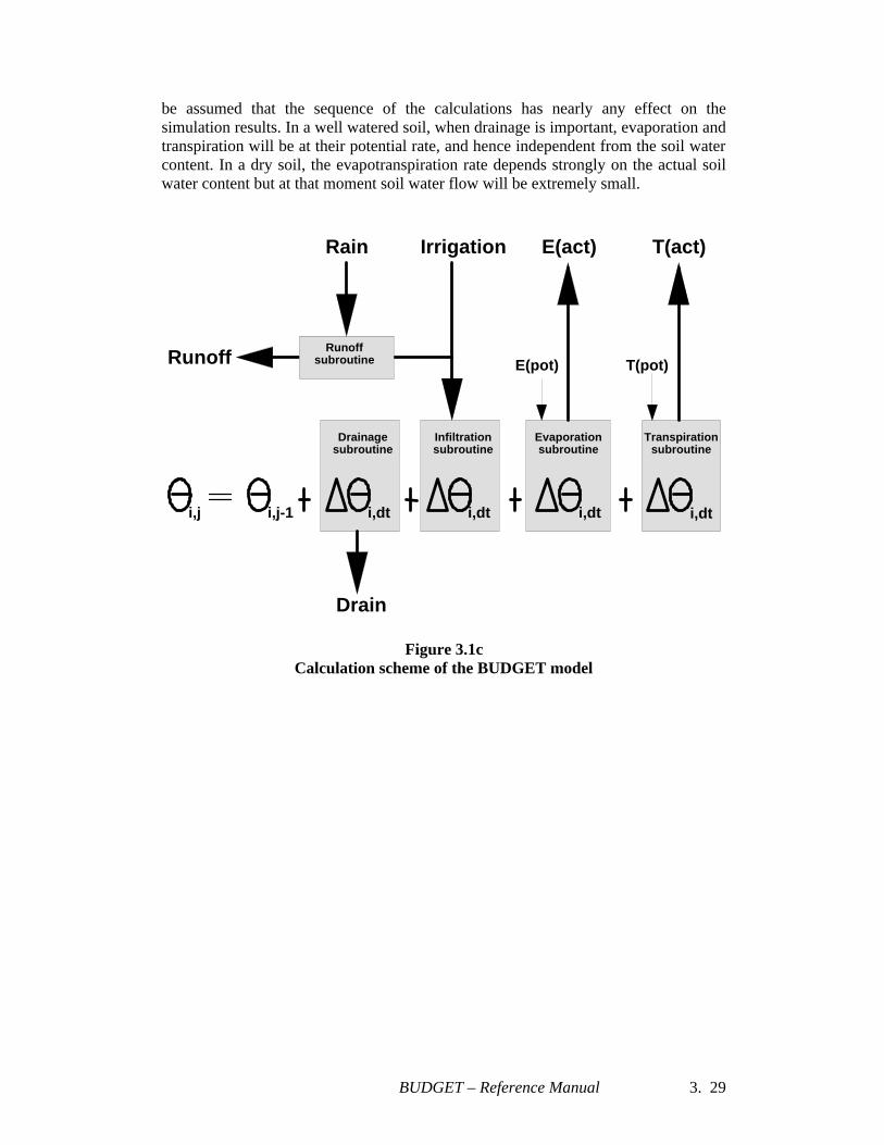
for the solution of the soil water balance with a soil water simulation model In BUDGET, the differential flow equation is replaced by a set of finite difference equations (subroutines), written in terms of the dependent variable θ (Fig. 3.1c). The simulation starts with the drainage of the soil profile. Subsequently water infiltrates into the soil profile (after the subtraction of surface runoff), and finally the amount of water lost by evaporation and transpiration is calculated. In each of the described subroutines, the soil water content is updated at the end of the time step (j) and at each grid point (i), according to the calculated water content variation (∆θ). The final water content variation at the end of a time step is the result from various processes described in different subroutines. Since the soil water variation calculated in a subroutine, depends on the actual soil water content, the sequence of the calculations might theoretically have an influence on the final simulation result. However, since the time step is restricted to one day and the response of the process of water flow at a particular soil water content is quite different than the response of the process of water uptake and water extraction, it may
BUDGET – Reference Manual 3. 29
be assumed that the sequence of the calculations has nearly any effect on the simulation results. In a well watered soil, when drainage is important, evaporation and transpiration will be at their potential rate, and hence independent from the soil water content. In a dry soil, the evapotranspiration rate depends strongly on the actual soil water content but at that moment soil water flow will be extremely small.
Drain
Rain Irrigation
E(pot) T(pot)Runoff
i,j i,j-1 i,dt i,dt i,dt i,dt
Drainagesubroutine
Infiltrationsubroutine
Evaporationsubroutine
Transpirationsubroutine
E(act) T(act)
Runoffsubroutine
Figure 3.1c Calculation scheme of the BUDGET model
BUDGET – Reference Manual 3. 30
3.2 Drainage subroutine To simulate the drainage inside and the percolation out of a soil layer, and to simulate the infiltration of rainfall and/or irrigation, BUDGET makes use of a drainage function (Raes, 1982; Raes et al., 1988):
11
)(−−
−=∆
∆−
−
FCsat
FCi
ee
t FCsati
θθ
θθ
θθτθ
(3.2a)
Where ∆θi/∆t decrease in soil water content at depth i, during time step ∆t [m3.m-3.day-1] τ drainage characteristic [-] θi actual soil water content at depth i [m3.m-3] θSAT soil water content at saturation [m3.m-3] θFC soil water content at field capacity [m3.m-3] ∆t time step [day] note: IF θi = θFC THAN ∆θi/∆t = 0 IF θi = θSAT THAN ∆θi/∆t = τ (θSAT - θFC)
0 1 2 3 4 5 6 7 8 9 10
time (day)
soil
wat
er c
onte
nt
saturation
field capacity
0.4
1.0
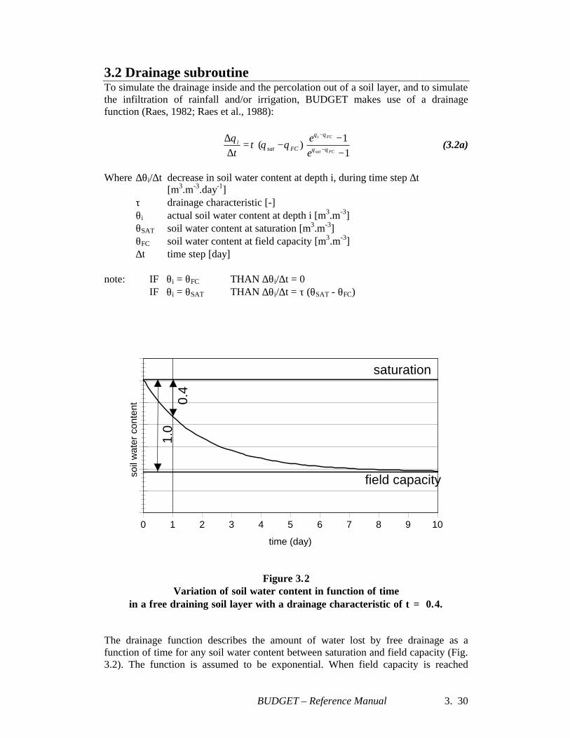
Figure 3.2
Variation of soil water content in function of time in a free draining soil layer with a drainage characteristic of τ = 0.4.
The drainage function describes the amount of water lost by free drainage as a function of time for any soil water content between saturation and field capacity (Fig. 3.2). The function is assumed to be exponential. When field capacity is reached
BUDGET – Reference Manual 3. 31
further drainage of the soil layer is disregarded. A drainage function is described by the dimensionless drainage characteristic τ (tau). The drainage function mimics quite realistic the infiltration and internal drainage as observed in the field (Raes, 1982; Feyen, 1987; Hess, 1999; Wiyo, 1999; Barrios Gonzales, 1999). The drainage characteristic (τ) expresses the decrease in soil water content of a soil layer, originally at saturation, at the end of the first day of free drainage. It is expressed as a fraction of the total drainable amount of water, which is the water content between saturation and field capacity. The value of τ may vary between 1 (complete drainage after one day) and 0 (impermeable soil layer). The larger τ, the faster the soil layer will reach field capacity. A coarse textured sandy soil layer has a large τ while the τ value for a heavy clay layer is very small (See Annex II for indicative values for various soil layers). In a uniform soil equally wet it can be assumed that the decrease in soil water content per day (∆θ/∆t) is constant throughout the draining profile. Given the actual soil water content the corresponding drainage ability ∆θ/∆t (m3.m-3.day-1) is given by Eq. 3.2a. The amount of water D (mm), which drains out of the soil profile at the end of each day, is given by:
tzt
D ∆∆∆∆
=θ
1000 (3.2b)
where θ the soil water content (m3.m-3) of the draining soil profile
∆z the thickness (m) of the draining soil profile ∆t the time step (1 day)
To simulate the process in a soil profile composed of various soil compartments, which are not necessarily equally wet and may belong to soil layers with different drainage characteristics, the calculation procedure consists in a comparison of the actual drainage ability of the different soil compartments. The drainage ability for any soil water content between saturation and field capacity is given by Eq. 3.2a. The drainage ability is zero when the soil water content is lower than or equal to field capacity. Given the soil water content of compartment 1, the decrease in soil water content during time step ∆t is given by Eq. 3.2a. The amount of water D1 (mm) that drains out of the top compartment at the end of a time step is given by:
tzt
D ∆∆∆
∆= 1
11 1000
θ (3.2c)
where D1 the flux between compartment 1 and 2
θ1 the soil water content (m3.m-3) of the top compartment ∆z1 the thickness (m) of the top compartment ∆t the time step (1 day)
Subsequently the soil water content of the top compartment is updated. The same calculations are repeated for the successive compartments. It is thereby assumed that

BUDGET – Reference Manual 3. 32
the cumulative drainage amount ΣDi = D1 + D2 + … will pass through any compartment as long as its drainage ability is greater than or equal to the drainage ability of the upperlying compartment. By comparing drainage abilities and not soil water contents, the calculation procedure is independently of the soil layer to which succeeding compartments may belong. If a compartment is reached which drainage ability is smaller than the upperlying compartment, ΣDi will be stored in that compartment, thereby increasing its soil water content and its drainage ability. If the soil water content of the compartment becomes thereby as high that its drainage ability becomes equal to the drainage ability of the upperlying compartment, the excess of the cumulative drainage amount, increased with the calculated drainage amount Di of that compartment, will flow into the underlying compartment. If the entire cumulative drainage amount can be stored in a compartment without increasing its soil water in such a way that its drainage ability becomes equal to that of the upperlying compartment, only the calculated drainage amount of that compartment will be transferred to the underlying compartment. At the bottom of the soil profile, the remaining part of the cumulative drainage will drain out of the soil profile. In each compartment, the cumulative drainage amount ΣDi that passes through should be smaller than or equal to the maximum infiltration rate of the soil layer to which the soil compartment belongs. If not so, part of the ΣDi will be stored in that compartment, or if required in the compartments above, until the remaining part of ΣDi equals the infiltration rate of the soil layer.
BUDGET – Reference Manual 3. 33
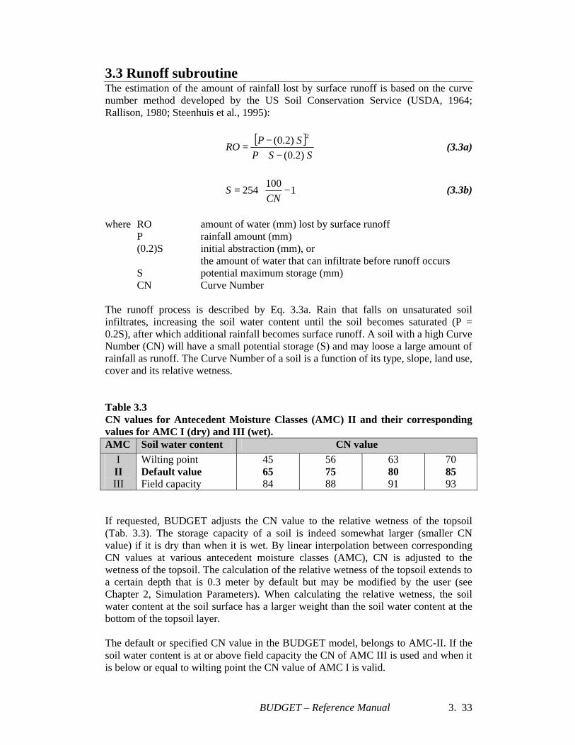
3.3 Runoff subroutine The estimation of the amount of rainfall lost by surface runoff is based on the curve number method developed by the US Soil Conservation Service (USDA, 1964; Rallison, 1980; Steenhuis et al., 1995):
[ ]SSP
SPRO
)2.0()2.0( 2
−+−
= (3.3a)
−= 1100
254CN
S (3.3b)
where RO amount of water (mm) lost by surface runoff P rainfall amount (mm) (0.2)S initial abstraction (mm), or
the amount of water that can infiltrate before runoff occurs S potential maximum storage (mm) CN Curve Number The runoff process is described by Eq. 3.3a. Rain that falls on unsaturated soil infiltrates, increasing the soil water content until the soil becomes saturated (P = 0.2S), after which additional rainfall becomes surface runoff. A soil with a high Curve Number (CN) will have a small potential storage (S) and may loose a large amount of rainfall as runoff. The Curve Number of a soil is a function of its type, slope, land use, cover and its relative wetness. Table 3.3 CN values for Antecedent Moisture Classes (AMC) II and their corresponding values for AMC I (dry) and III (wet). AMC Soil water content CN value
I II III
Wilting point Default value Field capacity
45 65 84
56 75 88
63 80 91
70 85 93
If requested, BUDGET adjusts the CN value to the relative wetness of the topsoil (Tab. 3.3). The storage capacity of a soil is indeed somewhat larger (smaller CN value) if it is dry than when it is wet. By linear interpolation between corresponding CN values at various antecedent moisture classes (AMC), CN is adjusted to the wetness of the topsoil. The calculation of the relative wetness of the topsoil extends to a certain depth that is 0.3 meter by default but may be modified by the user (see Chapter 2, Simulation Parameters). When calculating the relative wetness, the soil water content at the soil surface has a larger weight than the soil water content at the bottom of the topsoil layer. The default or specified CN value in the BUDGET model, belongs to AMC-II. If the soil water content is at or above field capacity the CN of AMC III is used and when it is below or equal to wilting point the CN value of AMC I is valid.
BUDGET – Reference Manual 3. 34
Current thinking (Hawkins (personal communication) 2002) is that the AMC-I and AMC-III CN’s are ‘error-bands’ to describe departure of surface runoff from all kind of sources, including soil moisture. There seems to be no much literature references to show real consistent impacts of prior soil water content on surface runoff on the scale proposed by USDA. Since irrigation is assumed to be fully controlled, the runoff subroutine is bypassed when irrigation water infiltrates into the soil. The maximum amount of water that can infiltrate into the soil, either as rainfall or irrigation, is however limited by the maximum infiltration rate of the topsoil layer. The fraction of the total applied amount of water larger than the infiltration rate if the topsoil, is always considered as lost by surface runoff. 3.4 Infiltration subroutine After the subtraction of surface runoff, the remaining part of the rainfall and irrigation water will infiltrate into the soil profile. In BUDGET the amount of water that infiltrates in the soil profile is stored into succeeding compartments from the top downwards, thereby not exceeding a threshold soil water content θ°i (m3.m-3). The threshold θ°i at a particular soil depth, depends on the infiltration rate of the corresponding soil layer and on the amount of infiltrated water that is not yet stored in the soil profile. The drainage rate at θ°i, should correspond with the amount of water that still has to pass through the compartment during the time step. If the flux exceeds the maximum infiltration rate of the corresponding soil layer (θ°i = θsat), extra water will be stored in the compartments above, until the remaining part, that has to pass through the compartment per unit of time step, is equal to the maximum infiltration rate. The calculation procedure is not completely independent of the thickness of the soil compartments. However, the simulation mimics quite realistic the infiltration process, by taking into account the initial wetness of the soil profile, the amount of water that infiltrates during the time step, the infiltration rate and drainage characteristics of the various soil layers of the soil profile.
BUDGET – Reference Manual 3. 35
3.5 Crop evapotranspiration 3.5.1 Evaporation power of the atmosphere The evaporation power of the atmosphere is expressed by the reference crop evapotranspriation ETo. The reference ETo incorporates the effects of various weather conditions on evapotranspiration. It can be derived by means of the FAO Penman-Monteith equation from climatic data from a nearby weather station or from pan evaporation (Allen et al., 1998). 3.5.2 Partitioning of ETcrop ETcrop is the evapotranspiration from a well-watered soil under the given climatic conditions. It is calculated by multiplying ETo by the crop coefficient Kc. The crop coefficient integrates the effect of characteristics that distinguish the cropped surface from the reference surface. It combines the effect of soil evaporation and crop transpiration. In BUDGET, ETcrop is calculated by assuming that the soil surface is wet from irrigation and rain. As such, ETcrop is the sum of the maximum amount of water that can be lost by soil evaporation (Epot) and by crop transpiration (Tpot):
TpotEpotETcrop += (3.5a) The maximum amount of water that might be lost by soil evaporation (Epot) is estimated by means of a Ritchie-type equation (Belmans et al., 1983):
ETcropefEpot LAIc−= (3.5b) where f and c are regression coefficient and LAI is the Leaf Area Index (m2.m-2). With f = 1.0 and c = 0.6 to 0.7 acceptable estimates of the potential soil evaporation may be obtained. The user can adjust the default values for the regression coefficients (see Chapter 2, Simulation Parameters). BUDGET contains sets of typical LAI values for various crop types. The user can adjust the generated LAI values at specific points of the growing season (see Chapter 2, Crop Parameters). When the soil is not cultivated (LAI = 0), Epot is given by multiplying ETo with Kcwet,bare soil. The default value for the Kc of a wet bare soil is 1.10 but can modified by the user (see Chapter 2, Simulation Parameters). To estimate the effect of mulches on the soil evaporation from non-cropped fields (before sowing/planting or after harvest), the general rule proposed by Allen et al. (1998) is applied:
EToKcSoilCover
Epot soilbarewet ,2100/(%)
1
−= (3.5c)
The potential crop transpiration (Tpot) is calculated by subtracting Epot from ETcrop. The division of ETcrop in Epot and Tpot is graphically displayed when running the BUDGET program (see Display/Update Crop Characteristics in the Main Menu).
BUDGET – Reference Manual 3. 36
3.5.3 Evaporation subroutine Water lost at the soil surface by evaporation is extracted from the topsoil. In BUDGET, the thickness of the topsoil is by default 0.4 meter but can be adjusted by the user (see Chapter 2, Simulation Parameters). Since soil water at the soil surface is more easily lost than at the bottom of the topsoil, weighting factors (fwz) are introduced. The sum of the weighting factors, which decrease exponentially from the soil surface to the bottom of the topsoil, is equal to one. The weighting factors determine the part of the atmospheric demand (Epot) that might be extracted from a particular soil depth. If at that depth the soil profile is wet, the requested amount of water is extracted (α = 1). But if the water content at a particular depth drops below a threshold, water cannot be extracted at that depth (α = 0). The threshold value, which is air dry, is half of the soil water content at wilting point. The actual soil evaporation is obtained by integrating equation 3.5d over the entire topsoil (z)
∫= dzEpotfwEact zα (3.5d)
3.5.4 Transpiration subroutine Water lost by transpiration is extracted out of the root zone. The root extraction term, S, expresses the amount of water that is extracted by the roots per unit of bulk volume of soil, per unit of time (m3.m-3.day-1). S, also denoted as the sink term, depends on a maximum sink term, Smax, and on the water stress factor Ks:
maxSKsS i = (3.5e) Where Si sink term (m3.m-3.day-1) of compartment i Ks water stress factor (dimensionless)
Smax maximum sink term (m3.m-3.day-1) By integrating Eq. 3.5e over the entire rooting depth, one obtains the actual transpiration rate Tact. The sum Σ(Si dz) can never exceeds Tpot. In BUDGET two options (see Chapter 2, Crop Parameters) are available to define the maximum sink term based on the solution methods presented by Feddes et al. (1978) and Hoogland et al. (1981). They correspond to one of the options for ‘Water uptake by plant roots’ (see Display/Update Crop parameters in Main Menu): - uniform over entire root zone (procedure by Feddes) - extraction pattern (procedure by Hoogland). When the first option is selected, Smax is calculated by dividing Tpot with the actual root depth. However, the calculated Smax should always be smaller than the specified maximum value. This implies that the water extraction over the entire root zone is uniformly distributed (when Ks = 1). When the second option is selected, Smax at the top of the soil profile might be different from Smax at the bottom of the root zone. With this option the water extraction may take place to a depth that might be less than the rooting depth. The water stress factor is equal to one in the range between the anaerobiosis point and a threshold soil water content (Fig. 3.5). When the soil water content is above the
BUDGET – Reference Manual 3. 37
anaerobiosis point, the root zone is water logged and Ks is smaller than one (after a time lag determined by the user).
0.00
0.20
0.40
0.60
0.80
1.00
Dr : root zone depletion (mm)
0 : soil water content (vol%)
Ks
0 0 0 0sat FC threshold WP
0.0 RAW TAW
anae
robi
osis
poi
nt
RAW
TAW
0.00air
Figure 3.5 The water stress factor Ks
The threshold value below which Ks becomes smaller than one is determined by the soil water depletion fraction for no stress (p). The p factor divides the Total Available soil Water (TAW), in two parts: water that can be extracted without stress (RAW) and water that is more difficult to extract. The threshold value is not a unique value but varies as a function of the evaporation demand. If the demand is low, p is somewhat larger then when it is high and hence more soil water can be transpired without inducing crop water stress. When the soil water content is below the threshold value, the water extracted is limited (Ks < 1) and the crop will be under water stress. The crop stress increases as the soil water content decreases. Water extraction becomes zero at Wilting Point. 3.5.5 Actual crop evapotranspiration (ETact) The actual crop evapotranspiration is the sum of the actual soil evaporation and actual crop transpiration
TactEactETact += (3.5f) ETact is smaller than or equal to ETcrop.
BUDGET – Reference Manual 3. 38
3.6 Estimation of Relative Yield Jensen (1968) proposed the following mathematical relationship between relative yield and the relative evapotranspiration:
iN
i i
i
ETcropETact
YmYa
λ
∏=
=
1
(3.6a)
where Ya is the actual harvested yield, Ym is the maximum crop yield under given management conditions that can be obtained when water is not limiting, N is the number of growth stages, ETacti is the actual evapotranspiration and ETcropi is evapotranspiration for non-limiting water conditions during the ith stage of growth and λi is the sensitivity index of crop to water stress during the ith stage of growth. The Jensen’s model has two advantages. The first advantage is that it integrates the effect of all the water stress throughout the growing season. The second advantage is that the model can be used at time steps less than a growth stage, for example an irrigation interval, if the cumulative procedure presented by Tsakiris (1982) is used. Doorenbos and Kassam (1979) empirically derived yield-response factors (Kyi) for individual growth stages (i.e. establishment, vegetative, flowering, yield formation, or ripening period) and also for the total growing period. These factors are yield response factors for water stress in specified physiological growth stage (i) and over the total growing period of crops, and are given by:
−=
−
i
ii ETcrop
ETactKy
YmYa
11 (3.6b)
where Kyi is the yield response factor to water stress. Eqn (3.6b) is valid for most crops for water deficits in the range (1-ETact/ETcrop ≤ 0.5). Sensitivity indexes of Jensen’s model are related to yield response factors by the following polynomial function (Kipkorir et al. 2002):
0187.08761.01351.02757.0 23 −+−= KyKyKyλ R2 = 0.99 (3.6c) For any given Ky value, the corresponding λ value can be derived with the help of Eqn (3.6c) for any given growth stage. The sensitivity indexes for shorter time period less than growth stage can be subsequently determined using the procedure presented by Tsakiris (1982). The effect of water stress on the relative yield during a short time period is finally derived by means of the Jensen model.
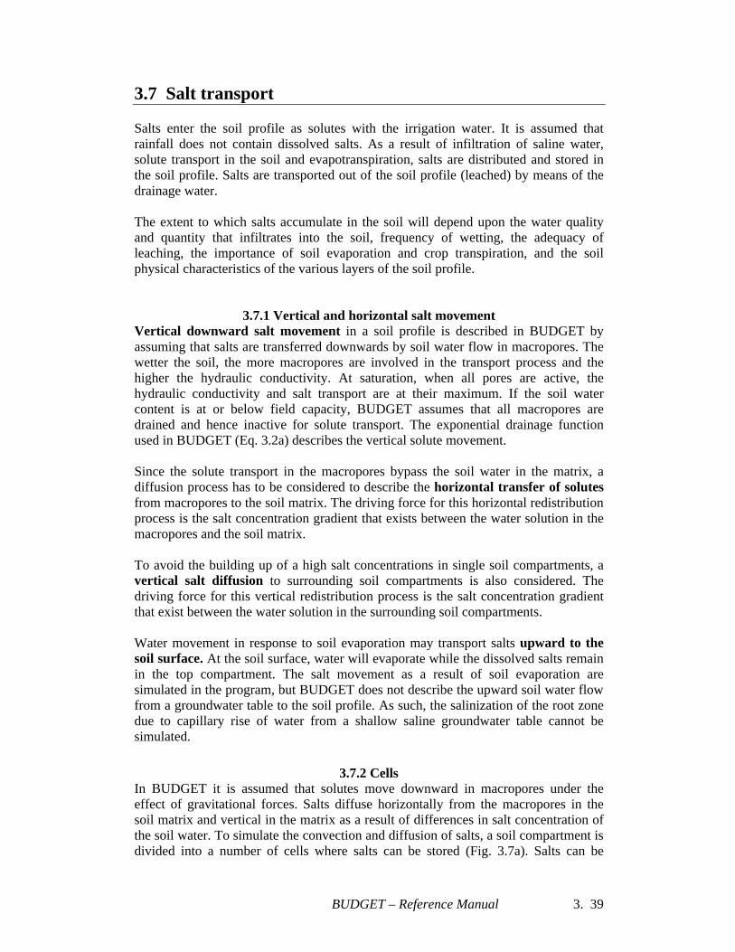
BUDGET – Reference Manual 3. 39
3.7 Salt transport Salts enter the soil profile as solutes with the irrigation water. It is assumed that rainfall does not contain dissolved salts. As a result of infiltration of saline water, solute transport in the soil and evapotranspiration, salts are distributed and stored in the soil profile. Salts are transported out of the soil profile (leached) by means of the drainage water. The extent to which salts accumulate in the soil will depend upon the water quality and quantity that infiltrates into the soil, frequency of wetting, the adequacy of leaching, the importance of soil evaporation and crop transpiration, and the soil physical characteristics of the various layers of the soil profile.
3.7.1 Vertical and horizontal salt movement Vertical downward salt movement in a soil profile is described in BUDGET by assuming that salts are transferred downwards by soil water flow in macropores. The wetter the soil, the more macropores are involved in the transport process and the higher the hydraulic conductivity. At saturation, when all pores are active, the hydraulic conductivity and salt transport are at their maximum. If the soil water content is at or below field capacity, BUDGET assumes that all macropores are drained and hence inactive for solute transport. The exponential drainage function used in BUDGET (Eq. 3.2a) describes the vertical solute movement. Since the solute transport in the macropores bypass the soil water in the matrix, a diffusion process has to be considered to describe the horizontal transfer of solutes from macropores to the soil matrix. The driving force for this horizontal redistribution process is the salt concentration gradient that exists between the water solution in the macropores and the soil matrix. To avoid the building up of a high salt concentrations in single soil compartments, a vertical salt diffusion to surrounding soil compartments is also considered. The driving force for this vertical redistribution process is the salt concentration gradient that exist between the water solution in the surrounding soil compartments. Water movement in response to soil evaporation may transport salts upward to the soil surface. At the soil surface, water will evaporate while the dissolved salts remain in the top compartment. The salt movement as a result of soil evaporation are simulated in the program, but BUDGET does not describe the upward soil water flow from a groundwater table to the soil profile. As such, the salinization of the root zone due to capillary rise of water from a shallow saline groundwater table cannot be simulated.
3.7.2 Cells In BUDGET it is assumed that solutes move downward in macropores under the effect of gravitational forces. Salts diffuse horizontally from the macropores in the soil matrix and vertical in the matrix as a result of differences in salt concentration of the soil water. To simulate the convection and diffusion of salts, a soil compartment is divided into a number of cells where salts can be stored (Fig. 3.7a). Salts can be
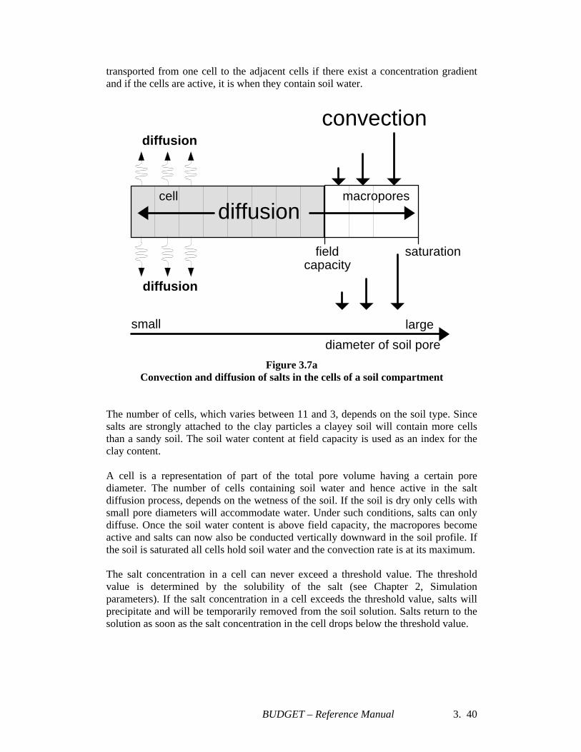
BUDGET – Reference Manual 3. 40
transported from one cell to the adjacent cells if there exist a concentration gradient and if the cells are active, it is when they contain soil water.
diffusion
convection
macroporescell
fieldcapacity
saturation
diameter of soil pore
small large
diffusion
diffusion
Figure 3.7a
Convection and diffusion of salts in the cells of a soil compartment The number of cells, which varies between 11 and 3, depends on the soil type. Since salts are strongly attached to the clay particles a clayey soil will contain more cells than a sandy soil. The soil water content at field capacity is used as an index for the clay content. A cell is a representation of part of the total pore volume having a certain pore diameter. The number of cells containing soil water and hence active in the salt diffusion process, depends on the wetness of the soil. If the soil is dry only cells with small pore diameters will accommodate water. Under such conditions, salts can only diffuse. Once the soil water content is above field capacity, the macropores become active and salts can now also be conducted vertically downward in the soil profile. If the soil is saturated all cells hold soil water and the convection rate is at its maximum. The salt concentration in a cell can never exceed a threshold value. The threshold value is determined by the solubility of the salt (see Chapter 2, Simulation parameters). If the salt concentration in a cell exceeds the threshold value, salts will precipitate and will be temporarily removed from the soil solution. Salts return to the solution as soon as the salt concentration in the cell drops below the threshold value.
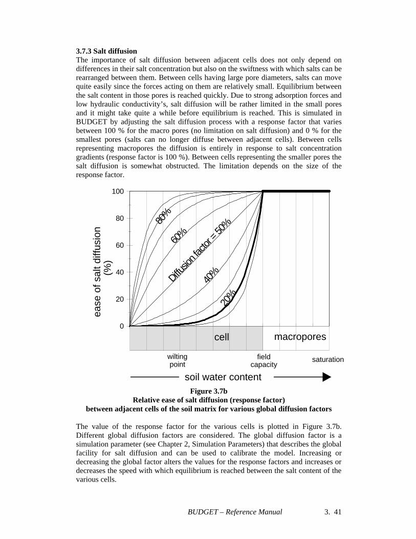
BUDGET – Reference Manual 3. 41
3.7.3 Salt diffusion The importance of salt diffusion between adjacent cells does not only depend on differences in their salt concentration but also on the swiftness with which salts can be rearranged between them. Between cells having large pore diameters, salts can move quite easily since the forces acting on them are relatively small. Equilibrium between the salt content in those pores is reached quickly. Due to strong adsorption forces and low hydraulic conductivity’s, salt diffusion will be rather limited in the small pores and it might take quite a while before equilibrium is reached. This is simulated in BUDGET by adjusting the salt diffusion process with a response factor that varies between 100 % for the macro pores (no limitation on salt diffusion) and 0 % for the smallest pores (salts can no longer diffuse between adjacent cells). Between cells representing macropores the diffusion is entirely in response to salt concentration gradients (response factor is 100 %). Between cells representing the smaller pores the salt diffusion is somewhat obstructed. The limitation depends on the size of the response factor.
0
20
40
60
80
100
ease
of s
alt d
iffus
ion
(%)
60%
80%
Diffusio
n fac
tor =
50%
macropores
soil water content
fieldcapacity
saturation
20%
40%
wiltingpoint
cell
Figure 3.7b
Relative ease of salt diffusion (response factor) between adjacent cells of the soil matrix for various global diffusion factors
The value of the response factor for the various cells is plotted in Figure 3.7b. Different global diffusion factors are considered. The global diffusion factor is a simulation parameter (see Chapter 2, Simulation Parameters) that describes the global facility for salt diffusion and can be used to calibrate the model. Increasing or decreasing the global factor alters the values for the response factors and increases or decreases the speed with which equilibrium is reached between the salt content of the various cells.
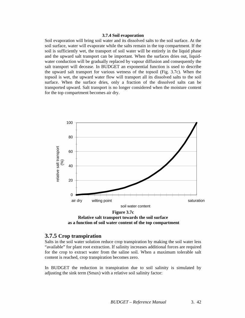
BUDGET – Reference Manual 3. 42
3.7.4 Soil evaporation
Soil evaporation will bring soil water and its dissolved salts to the soil surface. At the soil surface, water will evaporate while the salts remain in the top compartment. If the soil is sufficiently wet, the transport of soil water will be entirely in the liquid phase and the upward salt transport can be important. When the surfaces dries out, liquid-water conduction will be gradually replaced by vapour diffusion and consequently the salt transport will decease. In BUDGET an exponential function is used to describe the upward salt transport for various wetness of the topsoil (Fig. 3.7c). When the topsoil is wet, the upward water flow will transport all its dissolved salts to the soil surface. When the surface dries, only a fraction of the dissolved salts can be transported upward. Salt transport is no longer considered when the moisture content for the top compartment becomes air dry.
0
20
40
60
80
100
rela
tive
salt
tran
spor
t (%
)
air dry wilting point saturationsoil water content
Figure 3.7c Relative salt transport towards the soil surface
as a function of soil water content of the top compartment 3.7.5 Crop transpiration Salts in the soil water solution reduce crop transpiration by making the soil water less “available” for plant root extraction. If salinity increases additional forces are required for the crop to extract water from the saline soil. When a maximum tolerable salt content is reached, crop transpiration becomes zero. In BUDGET the reduction in transpiration due to soil salinity is simulated by adjusting the sink term (Smax) with a relative soil salinity factor:
BUDGET – Reference Manual 3. 43
−=
max1maxmax
ECeECsw
SS adjusted (3.7a)
Where Smax the maximum amount of water which can be taken up by the
roots per unit bulk volume of soil per unit of time [m3/m3.day], Smaxadjusted the value for Smax, adjusted to the soil salinity of the root zone
[m3/m3.day], ECsw the electrical conductivity of the soil water solution [dS/m], ECemax the electrical conductivity of the soil saturation extract at which
level crop yield is presumed to become zero [dS/m], Depending on the selected transpiration model (see Transpiration subroutine), a single value for Smax can be used over the entire root zone or Smax can be described as a function of the soil depth. The actual root extraction term, S, depends on the adjusted Smaxadjusted and the water stress factor Ks:
adjustedi SKsS max= (3.7b)
Where Si the sink term of compartment i [m3/m3.day], Ks water stress factor (0 .. 1)
The water stress factor Ks is a function of the soil moisture content and Smaxadjusted is a function of the salinity of the soil water solution and the salt tolerance of the crop. An increase in salt accumulation in the root and/or a reduction in soil water content increases the electrical conductivity of the soil water solution ECsw. An increase in ECsw increases the relative soil salinity (ECsw/ECemax) and reduces Smaxadjusted (the amount of water that can be potentially extracted by the roots). When the integration of Smaxadjusted over the entire root zone becomes smaller than the amount of water requested by transpiration (Tpot), the actual transpiration rate will be smaller than the potential value (Tact < Tpot). If the salt solution for the root zone is so saline that ECsw is equal to or larger than the maximum tolerable salt content for the given crop (ECemax), the relative soil salinity is 1 and crop transpiration ceases. Because some crops are better able to make the needed osmotic adjustments that enable them to extract more water from a saline soil, all plants do not respond to salinity in a similar manner. In Annex I Table 4, the electrical conductivity of the soil saturation extract at which point crop yield is presumed to become zero (ECemax) is given for many agricultural crops. Due to the linear relationship between seasonal crop yield reduction and crop water stress, ECemax is used in BUDGET to describe the reduction in crop transpiration due to salinity.
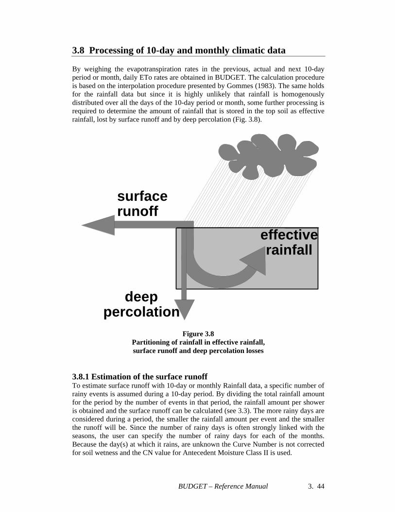
BUDGET – Reference Manual 3. 44
3.8 Processing of 10-day and monthly climatic data By weighing the evapotranspiration rates in the previous, actual and next 10-day period or month, daily ETo rates are obtained in BUDGET. The calculation procedure is based on the interpolation procedure presented by Gommes (1983). The same holds for the rainfall data but since it is highly unlikely that rainfall is homogenously distributed over all the days of the 10-day period or month, some further processing is required to determine the amount of rainfall that is stored in the top soil as effective rainfall, lost by surface runoff and by deep percolation (Fig. 3.8).
effectiverainfall
deep percolation
surfacerunoff
Figure 3.8 Partitioning of rainfall in effective rainfall, surface runoff and deep percolation losses
3.8.1 Estimation of the surface runoff To estimate surface runoff with 10-day or monthly Rainfall data, a specific number of rainy events is assumed during a 10-day period. By dividing the total rainfall amount for the period by the number of events in that period, the rainfall amount per shower is obtained and the surface runoff can be calculated (see 3.3). The more rainy days are considered during a period, the smaller the rainfall amount per event and the smaller the runoff will be. Since the number of rainy days is often strongly linked with the seasons, the user can specify the number of rainy days for each of the months. Because the day(s) at which it rains, are unknown the Curve Number is not corrected for soil wetness and the CN value for Antecedent Moisture Class II is used.
BUDGET – Reference Manual 3. 45
3.8.2 Estimation of effective rainfall Effective rainfall is that part of rainfall that is stored in the root zone and not lost by surface runoff or deep percolation (Fig. 3.8). If the rainfall data consist of 10-day or monthly values, the rainfall distribution over the period is unknown and the amount of water lost by deep percolation can not be determined by solving the water balance equation on a daily basis (time step). After the subtraction of the amount of rainfall lost by surface runoff, the effective rainfall is estimated by one or another procedure determined by the user. If the amount of rainfall that is stored in the root zone will also be effectively retained in the root zone depends on the storage capacity of the root zone at the moment of rainfall. The following procedures can be selected to determine the effective rainfall when 10-day or monthly rainfall data is used: a. 100 percent effective: All rainfall is stored in the root zone. b. USDA-SCS procedure: SCS scientists analysed 50 years of rainfall records at 22 locations throughout the United Sates of America to predict effective rainfall (SCS, 1993). A daily soil water balance incorporating crop evapotranspiration, rainfall, irrigation and the storage capacity of the root zone was used to determine the effective rainfall (Tab. 3.8). Simulations (Naesens, 2002) with rainfall data from various climatic zones indicates that the procedure predicts effective rainfall with an accuracy of +/- 20 %. The procedure is also valid for 10-day rainfall data but the accuracy decreases to +/- 40 %. c. Expressed as a percentage of rainfall: The user specifies the percentage of the 10-day/monthly rainfall that is stored in the root zone. The ineffective part of the rainfall is assumed to have drained out of the root zone and is stored immediately below the root zone. The percentage may vary over the season and will depend on the rainfall amount, the evapotranspiration rate and soil type. Indicative values are given in Table 3.8. The percentage can be obtained with greater accuracy by simulating the drainage out of the root zone for those years were daily rainfall data is available (or for a nearby representative station). As such the characteristics of the climate, cropping period, irrigation schedules and drainage characteristics of the soil can be fully considered.
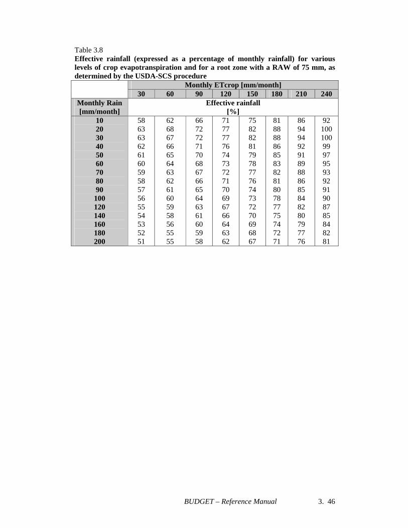
BUDGET – Reference Manual 3. 46
Table 3.8 Effective rainfall (expressed as a percentage of monthly rainfall) for various levels of crop evapotranspiration and for a root zone with a RAW of 75 mm, as determined by the USDA-SCS procedure
Monthly ETcrop [mm/month] 30 60 90 120 150 180 210 240
Monthly Rain [mm/month]
Effective rainfall [%]
10 20 30 40 50 60 70 80 90 100 120 140 160 180 200
58 63 63 62 61 60 59 58 57 56 55 54 53 52 51
62 68 67 66 65 64 63 62 61 60 59 58 56 55 55
66 72 72 71 70 68 67 66 65 64 63 61 60 59 58
71 77 77 76 74 73 72 71 70 69 67 66 64 63 62
75 82 82 81 79 78 77 76 74 73 72 70 69 68 67
81 88 88 86 85 83 82 81 80 78 77 75 74 72 71
86 94 94 92 91 89 88 86 85 84 82 80 79 77 76
92 100 100 99 97 95 93 92 91 90 87 85 84 82 81
BUDGET – Reference Manual References. 47
References Ahuja, L.R., D.K. Cassel, R.R. Bruce, and B.B. Barnes. 1989. Evaluation of spatial distribution of hydraulic conductivity using effective porosity data. Soil Science Journal. Vol. 148, N°6: 404-411. Allen, R., L.S. Pereira, D. Raes, and M. Smith. 1998. Crop evapotranspiration – Guidelines for computing crop water requirements. FAO Irrigation and Drainage Paper N° 56. Rome, Italy. 300 p. Barrios Gonzales, J.M. 1999. Comparative study of three approaches in the computation of soil water balance. Master Dissertation IUPWARE. K.U.Leuven University, Leuven, Belgium. 93 pp. Bear, J. 1972. Dynamics of fluids in porous media. American Elsevier, NY, USA: 338-346. Belmans, C., J.G. Wesseling and R.A. Feddes. 1983. Simulation of the water balance of a cropped soil: SWATRE. J. of Hydrol., 63: 271-286. Carnahan, B., H.A. Luther, and J.O. Wilkes. 1969. Applied numerical methods. John Wiley & Sons Inc., NY, USA: 429-444. Doorenbos, J. and A.H. Kassam. 1979. Yield response to water. FAO Irrigation and Drainage Paper N° 33. FAO, Rome, Italy. 193 p. FAO. 1990. Guidelines for soil description. Rome, Italy. 69 p. Feddes, R.A., P.J. Kowalik, and H. Zaradny. 1978. Simulation of field water use and crop yield. Pudoc, Simulation Monographs, Wageningen, The Netherlands. 189 p. Feyen, J. 1987. Field validation of soil water and crop models. In J. Feyen (Ed.) Simulation models for cropping systems in relation to water management. Proceedings of a symposium in the Community programme for coordination of agricultural research, Nov. 1986, Louvain, Belgium. Office for Official Publications of the European Communities, Luxembourg: 105-131. Gommes, R.A. 1983. Pocket computers in agrometeorlogy. FAO Plant Production and Protection Paper N° 45. FAO, Rome, Italy. 140 p. Goris, K. and B. Samain. 2001. Sustainable irrigation in the Gaza Strip. MSc dissertation Fac. of Applied and Biological Sciences, K.U.Leuven, Leuven, Belgium. 156 pages Hess, T.M. 1999. The impact of climatic variability over the period 1961-1990 on the soil water balance of upland soils in the north East Arid Zone of Nigeria. Institute of Water and Environment, Cranfield University, Silsoe, UK. 166 p.
BUDGET – Reference Manual References. 48
Hoogland, J.C., C. Belmans and R.A. Feddes. 1981. Root water uptake model depending on soil water pressure heads and maximum water extraction rate. Acta Hort. 119: 123-135. Hindryckx, S. 2002. Guidelines for sustainable irrigation in Naivasha, Rift Valley Province, Kenya). MSc dissertation Fac. of Applied and Biological Sciences, K.U.Leuven, Leuven, Belgium. 108 p. Jensen, M. E. 1968. Water consumption by agricultural plants. Chap.1 in Water Deficits and Plant Growth, Vol II, T. T. Kozlowski, ed., Academic Press, New York., pp. 1-22. Jury, W.A., W.R. Gardner and W.H. Gardner, 1991. Soil Physics. Fifth Edition, John Wiley and Sons, Inc. 328 pp. Kipkorir, E.C. and D. Raes. 2002. Transformation of yield response factor into Jensen’s sensitivity index. (in preparation). Naesens, K. 2002. Berekening van effectieve neerslag en oppervlakkige afstroming in waterbalansmodellen. MSc dissertation Fac. of Applied and Biological Sciences, K.U.Leuven, Leuven, Belgium. 92 p. Raes, D. 1982. A summary simulation model of the water budget of a cropped soil. Dissertationes de Agricultura n° 122. K.U.Leuven University, Leuven, Belgium. 110 p. Raes, D., H. Lemmens, P. Van Aelst, M. Vanden Bulcke and M. Smith. 1988. IRSIS – Irrigation scheduling information system. Volume 1. Manual. K.U.Leuven, Dep. Land Management, Reference Manual 3. 199 p. Raes, D., B. Van Goidsenhoven, K. Goris, B. Samain, E. De Pauw, M. El Baba, K. Tubail, J. Ismael and E. De Nys. 2001. BUDGET, a management tool for assessing salt accumulation in the root zone under irrigation. 4th Inter Regional Conference on Environment-Water, ICID. 27-30 Aug., Fortaleza, Brazil: 244-252. Rallison, R.E.. 1980. Origin and evolution of the SCS runoff equation. Symp. On Watershed Management, ASCE, New York, N.Y.: 912-924. Rawls, W.J., D.L. Brakensiek, K.E. Saxton. 1982. Estimation of soil water properties. Transactions of the ASAE: 1316-1320. Ritchie, J.T. 1972. Model for predicting evaporation from a row crop with incomplete cover. Water Res. Research, 8: 1204-1213. Saxton, K.E., W.J. Rawls, J.S. Romberger, and R.I. Papendick. 1986. Estimating generalized soil-water characteristics from texture. Soil Sci. Soc. Am. J. Vol. 50(4):1031-1036.

BUDGET – Reference Manual References. 49
SCS. 1991. Soil-Plant-Water Relationships. National Engineering Handbook, Section 15 ‘Irrigation’, Chapter 1. Soil Conservation Service, US Dep. of Agriculture. Washington, USA. 56 p. SCS. 1993. Irrigation water requirements. National Engineering Handbook, Part 623. Soil Conservation Service, US Dep. of Agriculture. Washington, USA. 284 p. Smith, M. 1985. Irrigation scheduling and water distribution. Proceedings of ‘Les besoins en Eau des Cultures’. Conférence Internationale INRA – ICID. Paris, France: 497-510. Smith, M. 1990. CROPWAT- a computer program for irrigation planning and management. FAO Irrigation and Drainage Paper N° 46. FAO, Rome, Italy. 126 p. Steenhuis, T.S., M. Winchell, J. Rossing, J.A. Zollweg, and M.F. Walter. 1995. SCS Runoff equation revisited for variable-source runoff areas. Journal of Irrigation and Drainage Eng. 121(3): 234-238. Sumith, 2002. Evaluation of Budget Salt module. MSc dissertation IUPWARE, Leuven, Belgium. (in press) Tsakiris, G. P. 1982. A method for applying crop sensitivity factors in irrigation scheduling. Agric. Water Manage. 5: 335-343. USDA. 1964. Estimation of direct runoff from storm rainfall. National Engineering Handbook, Washington DC, USA. Section 4 Hydrology, Chapter 4: 1-24. Vanclooster M., P. Viaene, J. Diels and K. Christiaens. 1994. WAVE – A mathematical model for simulating water and agrochemicals in the soil and vadose environment. Reference & user's manual. Institute for Land and Water Management. K.U.Leuven. Van Genuchten, M. Th., F.J. Leij and S.R. Yates. 1991. The RETC code for quantifying the hydraulic functions of unsaturated soils. US. Salinity Laboratory, Riverside, California. 83 pp. Van Goidsenhoven, B. 2000. Studie van de verzilting in de Khanasser vallei, Syrië – Evaluatie van het zoutbalansmodel BUDGET. MSc dissertation, Fac. of Applied and Biological Sciences, K.U.Leuven, Leuven, Belgium. 140 p. Williams, R.D., and Ahuja, L.R. 1993. Using available water content with the one-parameter model to estimate soil water retention, Soil Science. Vol. 156 (6): 380-388. Wiyo, K.A. 1999. Effect of tied-ridging on soil water status and maize yield under Malawi conditions. Dissertationes de Agricultura N° 397. K.U.Leuven University, Leuven, Belgium. 200 p.

BUDGET – Reference Manual Annex 1. 50
ANNEX I Indicative values for
Crop parameters Tables: 1. Indicative values for lengths of crop development stages for various planting
periods and climatic regions. (Source: Allen et al., 1998) 2. Crop coefficients and mean maximum plant heights for non stressed, well-
managed crops in subhumid climates (RHmin ~ 45%, U2 ~ 2 m/s). (Source: Allen et al., 1998)
3. Indicative values for maximum effective rooting depth, and soil water depletion fraction for no stress for common crops. (Source: Allen et al., 1998)
4. Indicative values for maximum crop salt tolerance levels (ECemax) for various crops. (Source: Ayers and Westcot, 1976)
5. Yield response factors for various crops. (Source: Doorenbos and Kassam, 1998) Sources: Allen, R., L.S. Pereira, D. Raes, and M. Smith. 1998. Crop evapotranspiration – Guidelines for computing crop water requirements. FAO Irrigation and Drainage Paper N° 56. Rome, Italy. 300 p. Ayers, R.S., and D.W. Westcot. 1985. Water quality for agriculture. FAO Irrigation and Drainage Paper N° 29. Rome Italy. 174 p. Doorenbos, J. and A.H. Kassam. 1979. Yield response to water. FAO Irrigation and Drainage Paper N° 33. FAO, Rome, Italy. 193 p.
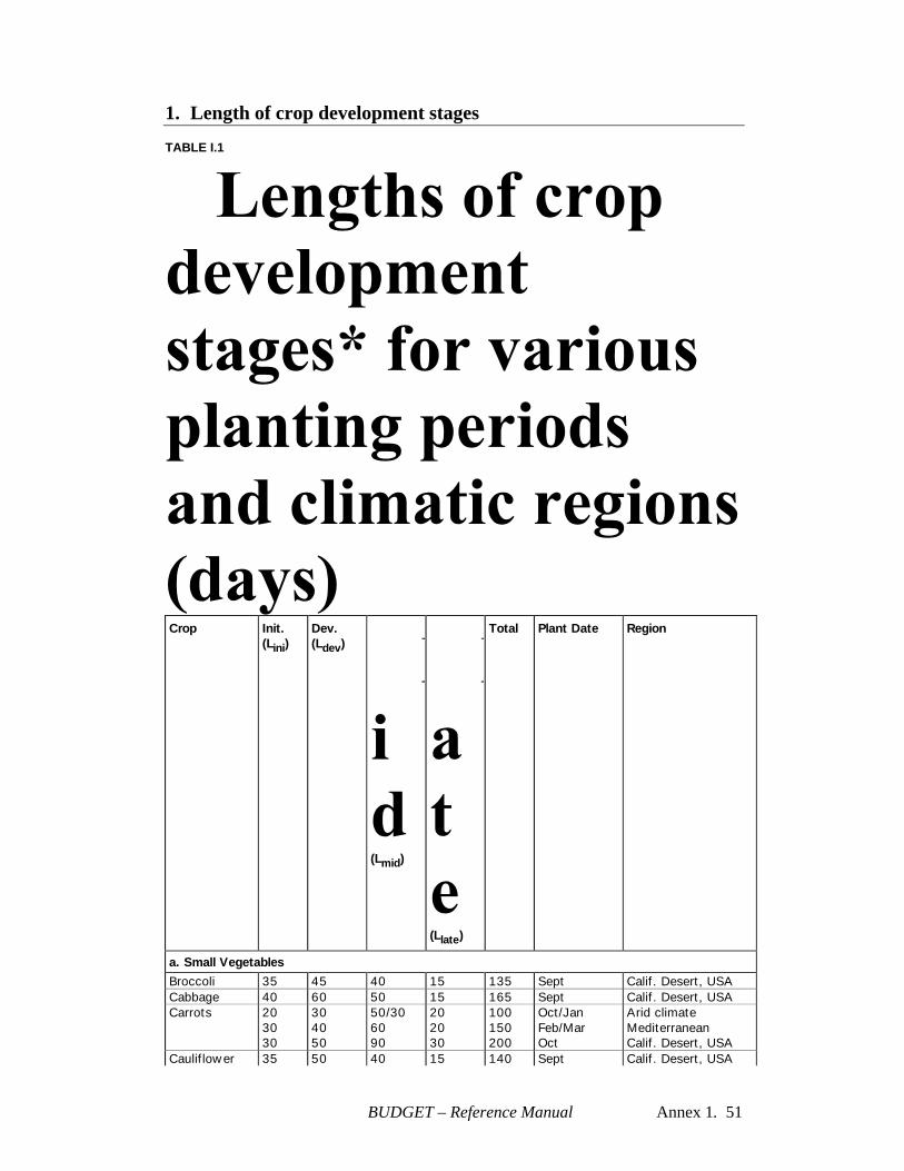
BUDGET – Reference Manual Annex 1. 51
1. Length of crop development stages
TABLE I.1
Crop Init. (Lini)
Dev. (Ldev)
(Lmid)
(Llate)
Total Plant Date Region
a. Small Vegetables Broccoli 35 45 40 15 135 Sept Calif. Desert, USA Cabbage 40 60 50 15 165 Sept Calif. Desert, USA Carrots 20
30 30
30 40 50
50/30 60 90
20 20 30
100 150 200
Oct/Jan Feb/Mar Oct
Arid climate Mediterranean Calif. Desert, USA
Cauliflower 35 50 40 15 140 Sept Calif. Desert, USA
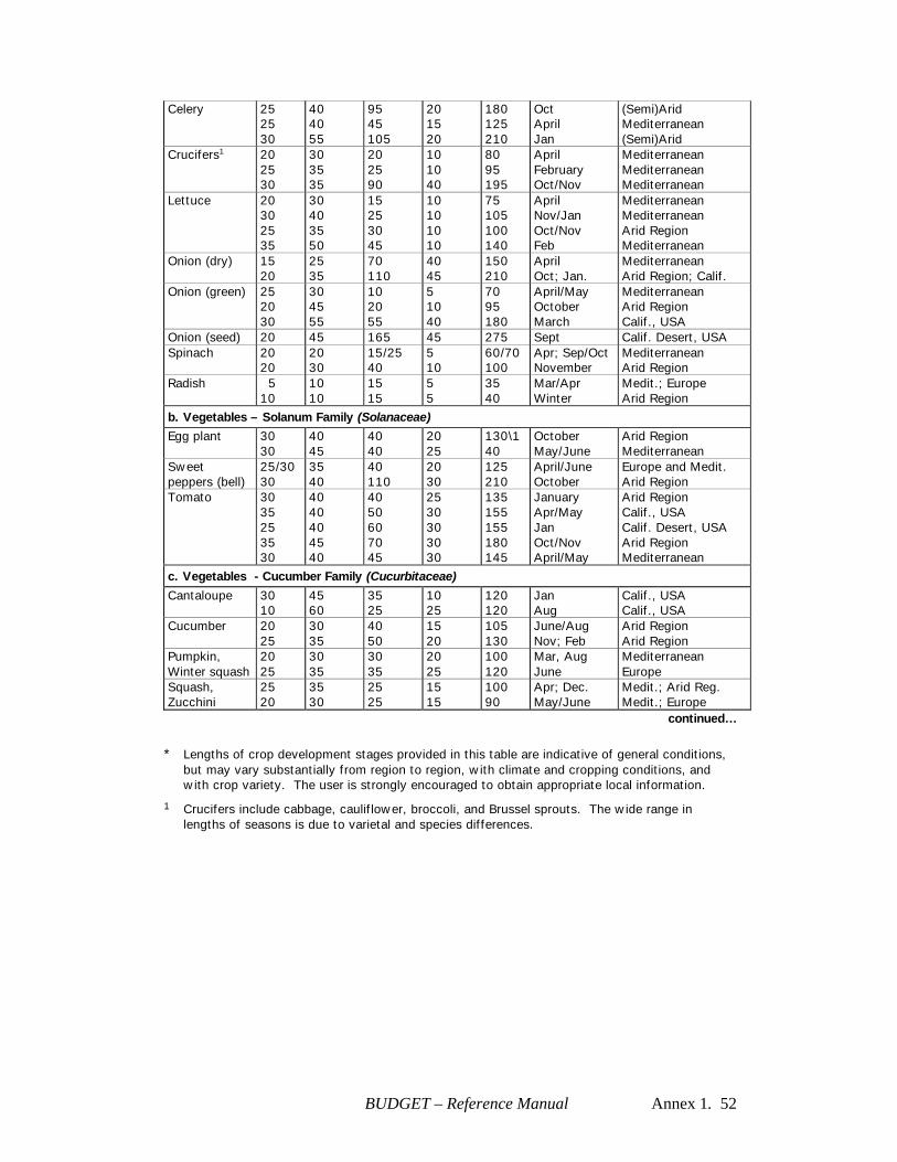
BUDGET – Reference Manual Annex 1. 52
Celery 25 25 30
40 40 55
95 45 105
20 15 20
180 125 210
Oct April Jan
(Semi)Arid Mediterranean (Semi)Arid
Crucifers1 20 25 30
30 35 35
20 25 90
10 10 40
80 95 195
April February Oct/Nov
Mediterranean Mediterranean Mediterranean
Lettuce 20 30 25 35
30 40 35 50
15 25 30 45
10 10 10 10
75 105 100 140
April Nov/Jan Oct/Nov Feb
Mediterranean Mediterranean Arid Region Mediterranean
Onion (dry) 15 20
25 35
70 110
40 45
150 210
April Oct; Jan.
Mediterranean Arid Region; Calif.
Onion (green) 25 20 30
30 45 55
10 20 55
5 10 40
70 95 180
April/May October March
Mediterranean Arid Region Calif., USA
Onion (seed) 20 45 165 45 275 Sept Calif. Desert, USA Spinach 20
20 20 30
15/25 40
5 10
60/70 100
Apr; Sep/Oct November
Mediterranean Arid Region
Radish 5 10
10 10
15 15
5 5
35 40
Mar/Apr Winter
Medit.; Europe Arid Region
b. Vegetables – Solanum Family (Solanaceae) Egg plant 30
30 40 45
40 40
20 25
130\140
October May/June
Arid Region Mediterranean
Sweet peppers (bell)
25/30 30
35 40
40 110
20 30
125 210
April/June October
Europe and Medit. Arid Region
Tomato 30 35 25 35 30
40 40 40 45 40
40 50 60 70 45
25 30 30 30 30
135 155 155 180 145
January Apr/May Jan Oct/Nov April/May
Arid Region Calif., USA Calif. Desert, USA Arid Region Mediterranean
c. Vegetables - Cucumber Family (Cucurbitaceae)
Cantaloupe 30 10
45 60
35 25
10 25
120 120
Jan Aug
Calif., USA Calif., USA
Cucumber 20 25
30 35
40 50
15 20
105 130
June/Aug Nov; Feb
Arid Region Arid Region
Pumpkin, Winter squash
20 25
30 35
30 35
20 25
100 120
Mar, Aug June
Mediterranean Europe
Squash, Zucchini
25 20
35 30
25 25
15 15
100 90
Apr; Dec. May/June
Medit.; Arid Reg. Medit.; Europe
continued…
* Lengths of crop development stages provided in this table are indicative of general conditions, but may vary substantially from region to region, with climate and cropping conditions, and with crop variety. The user is strongly encouraged to obtain appropriate local information.
1 Crucifers include cabbage, cauliflower, broccoli, and Brussel sprouts. The wide range in lengths of seasons is due to varietal and species differences.
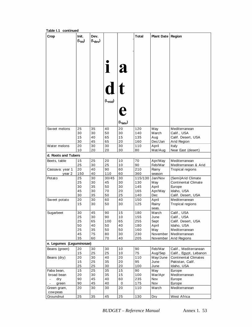
BUDGET – Reference Manual Annex 1. 53
Table I.1 continued
Crop Init. (Lini)
Dev. (Ldev)
(Lmid)
(Llate)
Total Plant Date Region
Sweet melons 25 30 15 30
35 30 40 45
40 50 65 65
20 30 15 20
120 140 135 160
May March Aug Dec/Jan
Mediterranean Calif., USA Calif. Desert, USA Arid Region
Water melons 20 10
30 20
30 20
30 30
110 80
April Mat/Aug
Italy Near East (desert)
d. Roots and Tubers Beets, table 15
25 25 30
20 25
10 10
70 90
Apr/May Feb/Mar
Mediterranean Mediterranean & Arid
Cassava: year 1 year 2
20 150
40 40
90 110
60 60
210 360
Rainy season
Tropical regions
Potato 25 25 30 45 30
30 30 35 30 35
30/45 45 50 70 50
30 30 30 20 25
115/130 130 145 165 140
Jan/Nov May April Apr/May Dec
(Semi)Arid Climate Continental Climate Europe Idaho, USA Calif. Desert, USA
Sweet potato 20 15
30 30
60 50
40 30
150 125
April Rainy seas.
Mediterranean Tropical regions
Sugarbeet 30 25 25 50 25 45 35
45 30 65 40 35 75 60
90 90 100 50 50 80 70
15 10 65 40 50 30 40
180 155 255 180 160 230 205
March June Sept April May November November
Calif., USA Calif., USA Calif. Desert, USA Idaho, USA Mediterranean Mediterranean Arid Regions
e. Legumes (Leguminosae) Beans (green) 20
15 30 25
30 25
10 10
90 75
Feb/Mar Aug/Sep
Calif., Mediterranean Calif., Egypt, Lebanon
Beans (dry) 20 15 25
30 25 25
40 35 30
20 20 20
110 95 100
May/June June June
Continental Climates Pakistan, Calif. Idaho, USA
Faba bean, broad bean
- dry - green
15 20 90 90
25 30 45 45
35 35 40 40
15 15 60 0
90 100 235 175
May Mar/Apr Nov Nov
Europe Mediterranean Europe Europe
Green gram, cowpeas
20 30 30 20 110 March Mediterranean
Groundnut 25 35 45 25 130 Dry West Africa
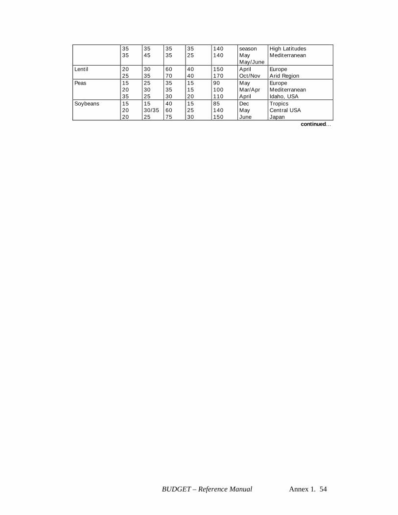
BUDGET – Reference Manual Annex 1. 54
35 35
35 45
35 35
35 25
140 140
season May May/June
High Latitudes Mediterranean
Lentil 20 25
30 35
60 70
40 40
150 170
April Oct/Nov
Europe Arid Region
Peas 15 20 35
25 30 25
35 35 30
15 15 20
90 100 110
May Mar/Apr April
Europe Mediterranean Idaho, USA
Soybeans 15 20 20
15 30/35 25
40 60 75
15 25 30
85 140 150
Dec May June
Tropics Central USA Japan
continued…
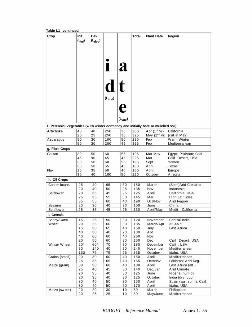
BUDGET – Reference Manual Annex 1. 55
Table I.1 continued.
Crop Init. (Lini)
Dev. (Ldev)
(Lmid)
(Llate)
Total Plant Date Region
f. Perennial Vegetables (with winter dormancy and initially bare or mulched soil) Artichoke 40
20 40 25
250 250
30 30
360 325
Apr (1st yr) May (2nd yr)
California (cut in May)
Asparagus 50 90
30 30
100 200
50 45
230 365
Feb Feb
Warm Winter Mediterranean
g. Fibre Crops Cotton 30
45 30 30
50 90 50 50
60 45 60 55
55 45 55 45
195 225 195 180
Mar-May Mar Sept April
Egypt; Pakistan; Calif. Calif. Desert, USA Yemen Texas
Flax 25 30
35 40
50 100
40 50
150 220
April October
Europe Arizona
h. Oil Crops Castor beans 25
20 40 40
65 50
50 25
180 135
March Nov.
(Semi)Arid Climates Indonesia
Safflower 20 25 35
35 35 55
45 55 60
25 30 40
125 145 190
April Mar Oct/Nov
California, USA High Latitudes Arid Region
Sesame 20 30 40 20 100 June China Sunflower 25 35 45 25 130 April/May Medit.; California i. Cereals Barley/Oats/ Wheat
15 20 15 40 40 20
25 25 30 30 60 50
50 60 65 40 60 60
30 30 40 20 40 30
120 135 150 130 200 160
November March/Apr July Apr Nov Dec
Central India 35-45 oL East Africa Calif. Desert, USA
Winter Wheat 202 30 160
602 140 75
70 40 75
30 30 25
180 240 335
December November October
Calif., USA Mediterranean Idaho, USA
Grains (small) 20 25
30 35
60 65
40 40
150 165
April Oct/Nov
Mediterranean Pakistan; Arid Reg.
Maize (grain) 30 25 20 20 30 30
50 40 35 35 40 40
60 45 40 40 50 50
40 30 30 30 30 50
180 140 125 125 150 170
April Dec/Jan June October April April
East Africa (alt.) Arid Climate Nigeria (humid) India (dry, cool) Spain (spr, sum.); Calif. Idaho, USA
Maize (sweet) 20 20
20 25
30 25
10 10
80 80
March May/June
Philippines Mediterranean

BUDGET – Reference Manual Annex 1. 56
20 30 20
30 30 40
50/30 30 70
10 103 10
90 110 140
Oct/Dec April Jan
Arid Climate Idaho, USA Calif. Desert, USA
Millet 15 20
25 30
40 55
25 35
105 140
June April
Pakistan Central USA
continued… 2 These periods for winter wheat will lengthen in frozen climates according to days having zero
growth potential and wheat dormancy . Under general conditions and in the absence of local data, fall planting of winter wheat can be presumed to occur in northern temperate climates when the 10-day running average of mean daily air temperature decreases to 17o C or December 1, whichever comes first. Planting of spring wheat can be presumed to occur when the 10-day running average of mean daily air temperature increases to 5o C. Spring planting of maize-grain can be presumed to occur when the 10-day running average of mean daily air temperature increases to 13o C.
3 The late season for sweet maize will be about 35 days if the grain is allowed to mature and dry.
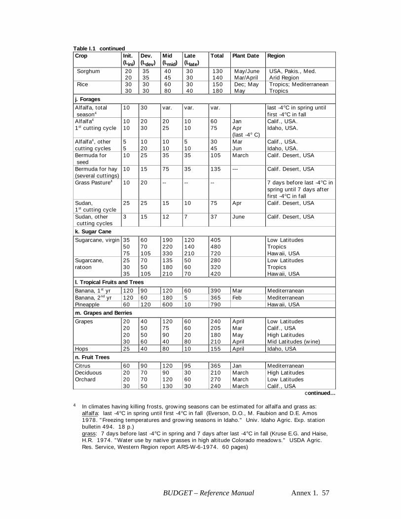
BUDGET – Reference Manual Annex 1. 57
Table I.1 continued Crop Init.
(Lini) Dev. (Ldev)
Mid (Lmid)
Late (Llate)
Total Plant Date Region
Sorghum 20 20
35 35
40 45
30 30
130 140
May/June Mar/April
USA, Pakis., Med. Arid Region
Rice 30 30
30 30
60 80
30 40
150 180
Dec; May May
Tropics; Mediterranean Tropics
j. Forages Alfalfa, total season4
10 30 var. var. var. last -4oC in spring until first -4oC in fall
Alfalfa4 1st cutting cycle
10 10
20 30
20 25
10 10
60 75
Jan Apr (last -4o C)
Calif., USA. Idaho, USA.
Alfalfa4, other cutting cycles
5 5
10 20
10 10
5 10
30 45
Mar Jun
Calif., USA. Idaho, USA.
Bermuda for seed
10 25 35 35 105 March Calif. Desert, USA
Bermuda for hay (several cuttings)
10 15 75 35 135 --- Calif. Desert, USA
Grass Pasture4 10 20 -- -- -- 7 days before last -4oC in spring until 7 days after first -4oC in fall
Sudan, 1st cutting cycle
25 25 15 10 75 Apr Calif. Desert, USA
Sudan, other cutting cycles
3 15 12 7 37 June Calif. Desert, USA
k. Sugar Cane Sugarcane, virgin 35
50 75
60 70 105
190 220 330
120 140 210
405 480 720
Low Latitudes Tropics Hawaii, USA
Sugarcane, ratoon
25 30 35
70 50 105
135 180 210
50 60 70
280 320 420
Low Latitudes Tropics Hawaii, USA
l. Tropical Fruits and Trees Banana, 1st yr 120 90 120 60 390 Mar Mediterranean Banana, 2nd yr 120 60 180 5 365 Feb Mediterranean Pineapple 60 120 600 10 790 Hawaii, USA m. Grapes and Berries
Grapes 20 20 20 30
40 50 50 60
120 75 90 40
60 60 20 80
240 205 180 210
April Mar May April
Low Latitudes Calif., USA High Latitudes Mid Latitudes (wine)
Hops 25 40 80 10 155 April Idaho, USA n. Fruit Trees
Citrus 60 90 120 95 365 Jan Mediterranean Deciduous Orchard
20 20 30
70 70 50
90 120 130
30 60 30
210 270 240
March March March
High Latitudes Low Latitudes Calif., USA
continued… 4 In climates having killing frosts, growing seasons can be estimated for alfalfa and grass as: alfalfa: last -4oC in spring until first -4oC in fall (Everson, D.O., M. Faubion and D.E. Amos
1978. "Freezing temperatures and growing seasons in Idaho." Univ. Idaho Agric. Exp. station bulletin 494. 18 p.)
grass: 7 days before last -4oC in spring and 7 days after last -4oC in fall (Kruse E.G. and Haise, H.R. 1974. "Water use by native grasses in high altitude Colorado meadows." USDA Agric. Res. Service, Western Region report ARS-W-6-1974. 60 pages)
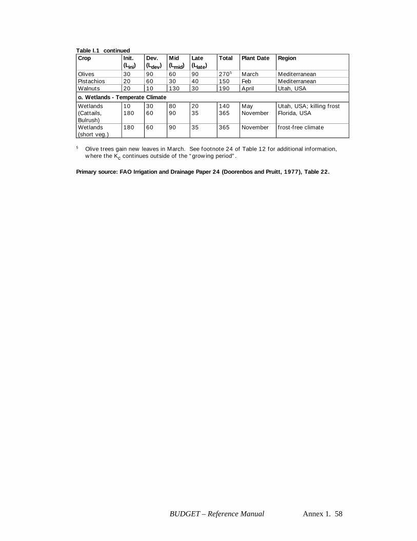
BUDGET – Reference Manual Annex 1. 58
Table I.1 continued Crop Init.
(Lini) Dev. (Ldev)
Mid (Lmid)
Late (Llate)
Total Plant Date Region
Olives 30 90 60 90 2705 March Mediterranean Pistachios 20 60 30 40 150 Feb Mediterranean Walnuts 20 10 130 30 190 April Utah, USA o. Wetlands - Temperate Climate Wetlands (Cattails, Bulrush)
10 180
30 60
80 90
20 35
140 365
May November
Utah, USA; killing frost Florida, USA
Wetlands (short veg.)
180 60 90 35 365 November frost-free climate
5 Olive trees gain new leaves in March. See footnote 24 of Table 12 for additional information,
where the Kc continues outside of the “growing period”. Primary source: FAO Irrigation and Drainage Paper 24 (Doorenbos and Pruitt, 1977), Table 22.
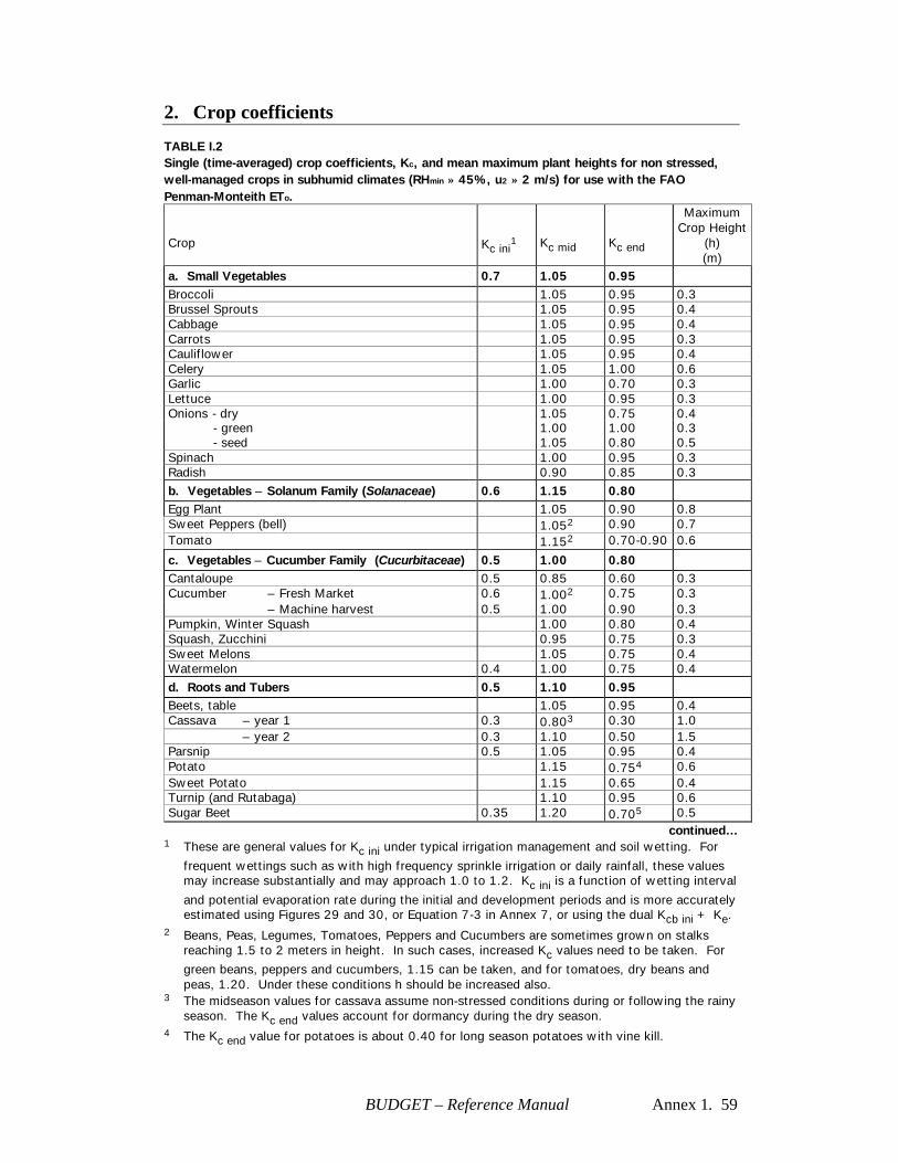
BUDGET – Reference Manual Annex 1. 59
2. Crop coefficients TABLE I.2 Single (time-averaged) crop coefficients, Kc, and mean maximum plant heights for non stressed, well-managed crops in subhumid climates (RHmin ≈ 45%, u2 ≈ 2 m/s) for use with the FAO Penman-Monteith ETo. Crop
Kc ini
1
Kc mid
Kc end
Maximum Crop Height
(h) (m)
a. Small Vegetables 0.7 1.05 0.95 Broccoli 1.05 0.95 0.3 Brussel Sprouts 1.05 0.95 0.4 Cabbage 1.05 0.95 0.4 Carrots 1.05 0.95 0.3 Cauliflower 1.05 0.95 0.4 Celery 1.05 1.00 0.6 Garlic 1.00 0.70 0.3 Lettuce 1.00 0.95 0.3 Onions - dry 1.05 0.75 0.4
- green 1.00 1.00 0.3 - seed 1.05 0.80 0.5
Spinach 1.00 0.95 0.3 Radish 0.90 0.85 0.3 b. Vegetables – Solanum Family (Solanaceae) 0.6 1.15 0.80 Egg Plant 1.05 0.90 0.8 Sweet Peppers (bell) 1.052 0.90 0.7 Tomato 1.152 0.70-0.90 0.6
c. Vegetables – Cucumber Family (Cucurbitaceae) 0.5 1.00 0.80 Cantaloupe 0.5 0.85 0.60 0.3 Cucumber – Fresh Market 0.6 1.002 0.75 0.3 – Machine harvest 0.5 1.00 0.90 0.3 Pumpkin, Winter Squash 1.00 0.80 0.4 Squash, Zucchini 0.95 0.75 0.3 Sweet Melons 1.05 0.75 0.4 Watermelon 0.4 1.00 0.75 0.4 d. Roots and Tubers 0.5 1.10 0.95 Beets, table 1.05 0.95 0.4 Cassava – year 1 0.3 0.803 0.30 1.0 – year 2 0.3 1.10 0.50 1.5 Parsnip 0.5 1.05 0.95 0.4 Potato 1.15 0.754 0.6 Sweet Potato 1.15 0.65 0.4 Turnip (and Rutabaga) 1.10 0.95 0.6 Sugar Beet 0.35 1.20 0.705 0.5
continued…
1 These are general values for Kc ini under typical irrigation management and soil wetting. For
frequent wettings such as with high frequency sprinkle irrigation or daily rainfall, these values may increase substantially and may approach 1.0 to 1.2. Kc ini is a function of wetting interval
and potential evaporation rate during the initial and development periods and is more accurately estimated using Figures 29 and 30, or Equation 7-3 in Annex 7, or using the dual Kcb ini + Ke.
2 Beans, Peas, Legumes, Tomatoes, Peppers and Cucumbers are sometimes grown on stalks reaching 1.5 to 2 meters in height. In such cases, increased Kc values need to be taken. For green beans, peppers and cucumbers, 1.15 can be taken, and for tomatoes, dry beans and peas, 1.20. Under these conditions h should be increased also.
3 The midseason values for cassava assume non-stressed conditions during or following the rainy season. The Kc end values account for dormancy during the dry season.
4 The Kc end value for potatoes is about 0.40 for long season potatoes with vine kill.

BUDGET – Reference Manual Annex 1. 60
5 This Kc end value is for no irrigation during the last month of the growing season. The Kc end
value for sugar beets is higher, up to 1.0, when irrigation or significant rain occurs during the last month.
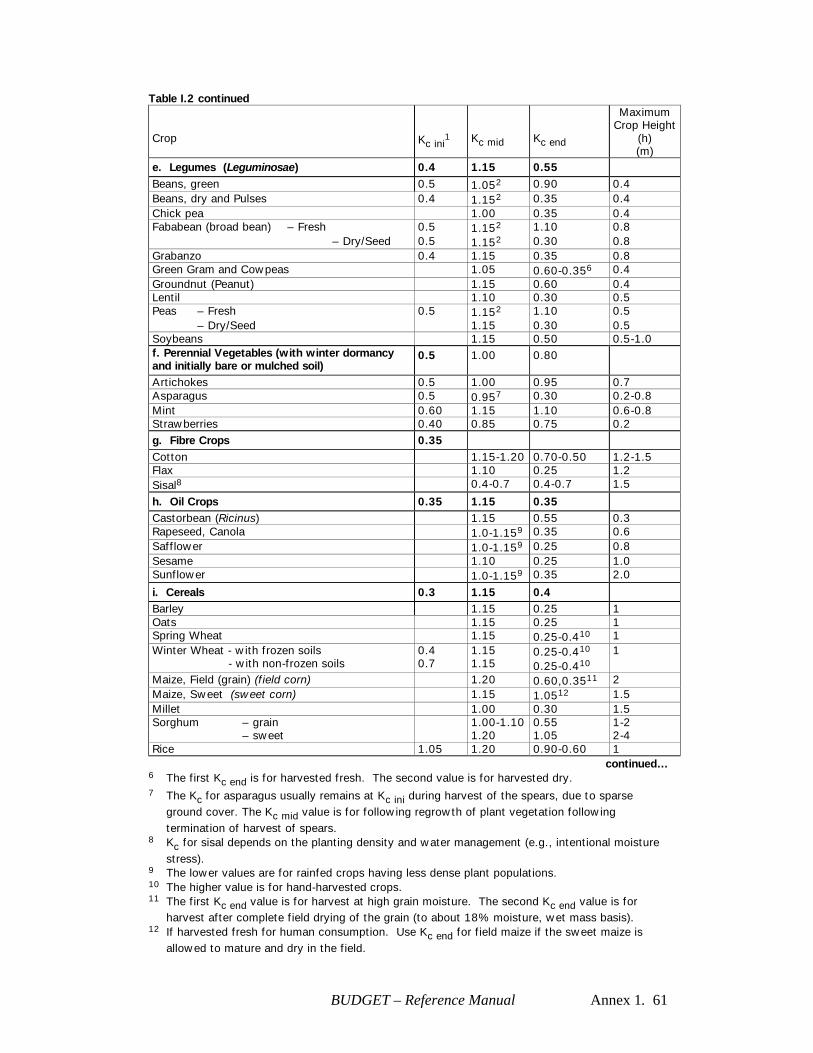
BUDGET – Reference Manual Annex 1. 61
Table I.2 continued Crop
Kc ini
1
Kc mid
Kc end
Maximum Crop Height
(h) (m)
e. Legumes (Leguminosae) 0.4 1.15 0.55 Beans, green 0.5 1.052 0.90 0.4 Beans, dry and Pulses 0.4 1.152 0.35 0.4 Chick pea 1.00 0.35 0.4 Fababean (broad bean) – Fresh 0.5 1.152 1.10 0.8 – Dry/Seed 0.5 1.152 0.30 0.8 Grabanzo 0.4 1.15 0.35 0.8 Green Gram and Cowpeas 1.05 0.60-0.356 0.4 Groundnut (Peanut) 1.15 0.60 0.4 Lentil 1.10 0.30 0.5 Peas – Fresh 0.5 1.152 1.10 0.5 – Dry/Seed 1.15 0.30 0.5 Soybeans 1.15 0.50 0.5-1.0 f. Perennial Vegetables (with winter dormancy and initially bare or mulched soil)
0.5 1.00 0.80
Artichokes 0.5 1.00 0.95 0.7 Asparagus 0.5 0.957 0.30 0.2-0.8 Mint 0.60 1.15 1.10 0.6-0.8 Strawberries 0.40 0.85 0.75 0.2 g. Fibre Crops 0.35 Cotton 1.15-1.20 0.70-0.50 1.2-1.5 Flax 1.10 0.25 1.2 Sisal8 0.4-0.7 0.4-0.7 1.5
h. Oil Crops 0.35 1.15 0.35 Castorbean (Ricinus) 1.15 0.55 0.3 Rapeseed, Canola 1.0-1.159 0.35 0.6 Safflower 1.0-1.159 0.25 0.8 Sesame 1.10 0.25 1.0 Sunflower 1.0-1.159 0.35 2.0
i. Cereals 0.3 1.15 0.4 Barley 1.15 0.25 1 Oats 1.15 0.25 1 Spring Wheat 1.15 0.25-0.410 1 Winter Wheat - with frozen soils
- with non-frozen soils 0.4 0.7
1.15 1.15
0.25-0.410
0.25-0.410 1
Maize, Field (grain) (field corn) 1.20 0.60,0.3511 2 Maize, Sweet (sweet corn) 1.15 1.0512 1.5 Millet 1.00 0.30 1.5 Sorghum – grain 1.00-1.10 0.55 1-2 – sweet 1.20 1.05 2-4 Rice 1.05 1.20 0.90-0.60 1
continued… 6 The first Kc end is for harvested fresh. The second value is for harvested dry. 7 The Kc for asparagus usually remains at Kc ini during harvest of the spears, due to sparse
ground cover. The Kc mid value is for following regrowth of plant vegetation following termination of harvest of spears.
8 Kc for sisal depends on the planting density and water management (e.g., intentional moisture stress).
9 The lower values are for rainfed crops having less dense plant populations. 10 The higher value is for hand-harvested crops. 11 The first Kc end value is for harvest at high grain moisture. The second Kc end value is for
harvest after complete field drying of the grain (to about 18% moisture, wet mass basis). 12 If harvested fresh for human consumption. Use Kc end for field maize if the sweet maize is
allowed to mature and dry in the field.
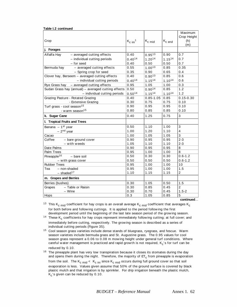
BUDGET – Reference Manual Annex 1. 62
Table I.2 continued Crop
Kc ini
1
Kc mid
Kc end
Maximum Crop Height
(h) (m)
j. Forages Alfalfa Hay – averaged cutting effects 0.40 0.9513 0.90 0.7 – individual cutting periods 0.4014 1.2014 1.1514 0.7 – for seed 0.40 0.50 0.50 0.7 Bermuda hay – averaged cutting effects 0.55 1.0013 0.85 0.35 – Spring crop for seed 0.35 0.90 0.65 0.4 Clover hay, Berseem – averaged cutting effects 0.40 0.9013 0.85 0.6 – individual cutting periods 0.4014 1.1514 1.1014 0.6 Rye Grass hay – averaged cutting effects 0.95 1.05 1.00 0.3 Sudan Grass hay (annual) – averaged cutting effects 0.50 0.9014 0.85 1.2 – individual cutting periods 0.5014 1.1514 1.1014 1.2 Grazing Pasture - Rotated Grazing 0.40 0.85-1.05 0.85 0.15-0.30
- Extensive Grazing 0.30 0.75 0.75 0.10 Turf grass - cool season15 0.90 0.95 0.95 0.10
- warm season15 0.80 0.85 0.85 0.10
k. Sugar Cane 0.40 1.25 0.75 3
l. Tropical Fruits and Trees
Banana – 1st year 0.50 1.10 1.00 3 – 2nd year 1.00 1.20 1.10 4 Cacao 1.00 1.05 1.05 3 Coffee – bare ground cover 0.90 0.95 0.95 2-3 – with weeds 1.05 1.10 1.10 2-3 Date Palms 0.90 0.95 0.95 8 Palm Trees 0.95 1.00 1.00 8 Pineapple16 – bare soil 0.50 0.30 0.30 0.6-1.2 – with grass cover 0.50 0.50 0.50 0.6-1.2 Rubber Trees 0.95 1.00 1.00 10 Tea – non-shaded 0.95 1.00 1.00 1.5 – shaded17 1.10 1.15 1.15 2
m. Grapes and Berries Berries (bushes) 0.30 1.05 0.50 1.5 Grapes – Table or Raisin 0.30 0.85 0.45 2 – Wine 0.30 0.70 0.45 1.5-2 Hops 0.3 1.05 0.85 5
continued… 13 This Kc mid coefficient for hay crops is an overall average Kc mid coefficient that averages Kc
for both before and following cuttings. It is applied to the period following the first development period until the beginning of the last late season period of the growing season.
14 These Kc coefficients for hay crops represent immediately following cutting; at full cover; and
immediately before cutting, respectively. The growing season is described as a series of individual cutting periods (Figure 35).
15 Cool season grass varieties include dense stands of bluegrass, ryegrass, and fescue. Warm season varieties include bermuda grass and St. Augustine grass. The 0.95 values for cool season grass represent a 0.06 to 0.08 m mowing height under general turf conditions. Where careful water management is practiced and rapid growth is not required, Kc's for turf can be reduced by 0.10.
16 The pineapple plant has very low transpiration because it closes its stomates during the day and opens them during the night. Therefore, the majority of ETc from pineapple is evaporation from the soil. The Kc mid < Kc ini since Kc mid occurs during full ground cover so that soil evaporation is less. Values given assume that 50% of the ground surface is covered by black plastic mulch and that irrigation is by sprinkler. For drip irrigation beneath the plastic mulch, Kc's given can be reduced by 0.10.

BUDGET – Reference Manual Annex 1. 63
17 Includes the water requirements of the shade trees.
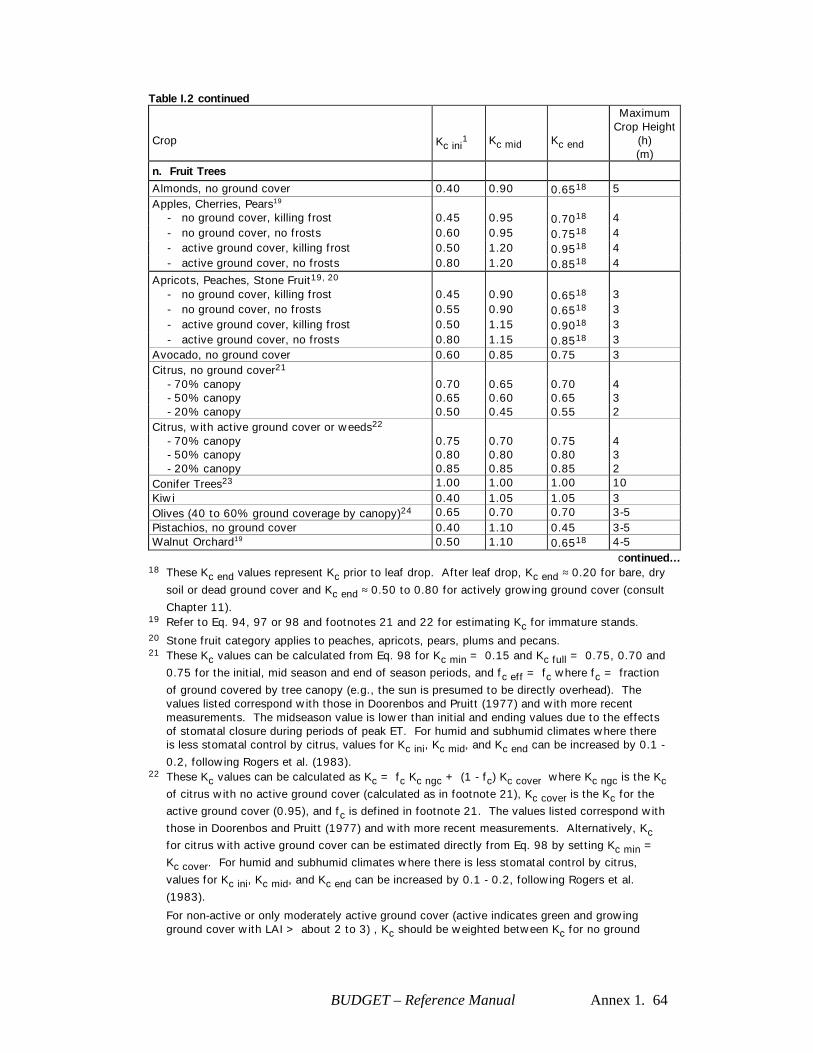
BUDGET – Reference Manual Annex 1. 64
Table I.2 continued Crop
Kc ini
1
Kc mid
Kc end
Maximum Crop Height
(h) (m)
n. Fruit Trees Almonds, no ground cover 0.40 0.90 0.6518 5 Apples, Cherries, Pears19 - no ground cover, killing frost 0.45 0.95 0.7018 4 - no ground cover, no frosts 0.60 0.95 0.7518 4 - active ground cover, killing frost 0.50 1.20 0.9518 4 - active ground cover, no frosts 0.80 1.20 0.8518 4 Apricots, Peaches, Stone Fruit19, 20 - no ground cover, killing frost 0.45 0.90 0.6518 3 - no ground cover, no frosts 0.55 0.90 0.6518 3 - active ground cover, killing frost 0.50 1.15 0.9018 3 - active ground cover, no frosts 0.80 1.15 0.8518 3 Avocado, no ground cover 0.60 0.85 0.75 3 Citrus, no ground cover21 - 70% canopy 0.70 0.65 0.70 4 - 50% canopy 0.65 0.60 0.65 3 - 20% canopy 0.50 0.45 0.55 2 Citrus, with active ground cover or weeds22 - 70% canopy 0.75 0.70 0.75 4 - 50% canopy 0.80 0.80 0.80 3 - 20% canopy 0.85 0.85 0.85 2 Conifer Trees23 1.00 1.00 1.00 10 Kiwi 0.40 1.05 1.05 3 Olives (40 to 60% ground coverage by canopy)24 0.65 0.70 0.70 3-5 Pistachios, no ground cover 0.40 1.10 0.45 3-5 Walnut Orchard19 0.50 1.10 0.6518 4-5 continued… 18 These Kc end values represent Kc prior to leaf drop. After leaf drop, Kc end ≈ 0.20 for bare, dry
soil or dead ground cover and Kc end ≈ 0.50 to 0.80 for actively growing ground cover (consult
Chapter 11). 19 Refer to Eq. 94, 97 or 98 and footnotes 21 and 22 for estimating Kc for immature stands.
20 Stone fruit category applies to peaches, apricots, pears, plums and pecans. 21 These Kc values can be calculated from Eq. 98 for Kc min = 0.15 and Kc full = 0.75, 0.70 and
0.75 for the initial, mid season and end of season periods, and fc eff = fc where fc = fraction of ground covered by tree canopy (e.g., the sun is presumed to be directly overhead). The values listed correspond with those in Doorenbos and Pruitt (1977) and with more recent measurements. The midseason value is lower than initial and ending values due to the effects of stomatal closure during periods of peak ET. For humid and subhumid climates where there is less stomatal control by citrus, values for Kc ini, Kc mid, and Kc end can be increased by 0.1 - 0.2, following Rogers et al. (1983).
22 These Kc values can be calculated as Kc = fc Kc ngc + (1 - fc) Kc cover where Kc ngc is the Kc of citrus with no active ground cover (calculated as in footnote 21), Kc cover is the Kc for the active ground cover (0.95), and fc is defined in footnote 21. The values listed correspond with those in Doorenbos and Pruitt (1977) and with more recent measurements. Alternatively, Kc for citrus with active ground cover can be estimated directly from Eq. 98 by setting Kc min = Kc cover. For humid and subhumid climates where there is less stomatal control by citrus, values for Kc ini, Kc mid, and Kc end can be increased by 0.1 - 0.2, following Rogers et al. (1983).
For non-active or only moderately active ground cover (active indicates green and growing ground cover with LAI > about 2 to 3) , Kc should be weighted between Kc for no ground

BUDGET – Reference Manual Annex 1. 65
cover and Kc for active ground cover, with the weighting based on the "greenness" and approximate leaf area of the ground cover.
23 Confers exhibit substantial stomatal control due to reduced aerodynamic resistance. The Kc can easily reduce below the values presented, which represent well-watered conditions for large forests.
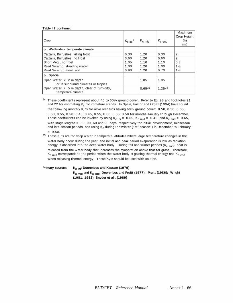
BUDGET – Reference Manual Annex 1. 66
Table I.2 continued Crop
Kc ini
1
Kc mid
Kc end
Maximum Crop Height
(h) (m)
o. Wetlands – temperate climate Cattails, Bulrushes, killing frost 0.30 1.20 0.30 2 Cattails, Bulrushes, no frost 0.60 1.20 0.60 2 Short Veg., no frost 1.05 1.10 1.10 0.3 Reed Swamp, standing water 1.00 1.20 1.00 1-3 Reed Swamp, moist soil 0.90 1.20 0.70 1-3 p. Special Open Water, < 2 m depth or in subhumid climates or tropics
1.05 1.05
Open Water, > 5 m depth, clear of turbidity, temperate climate
0.6525 1.2525
24 These coefficients represent about 40 to 60% ground cover. Refer to Eq. 98 and footnotes 21
and 22 for estimating Kc for immature stands. In Spain, Pastor and Orgaz (1994) have found the following monthly Kc‘s for olive orchards having 60% ground cover: 0.50, 0.50, 0.65, 0.60, 0.55, 0.50, 0.45, 0.45, 0.55, 0.60, 0.65, 0.50 for months January through December. These coefficients can be invoked by using Kc ini = 0.65, Kc mid = 0.45, and Kc end = 0.65,
with stage lengths = 30, 90, 60 and 90 days, respectively for initial, development, midseason and late season periods, and using Kc during the winter (“off season”) in December to February = 0.50.
25 These Kc's are for deep water in temperate latitudes where large temperature changes in the
water body occur during the year, and initial and peak period evaporation is low as radiation energy is absorbed into the deep water body. During fall and winter periods (Kc end), heat is
released from the water body that increases the evaporation above that for grass. Therefore, Kc mid corresponds to the period when the water body is gaining thermal energy and Kc end when releasing thermal energy. These Kc's should be used with caution.
Primary sources: Kc ini: Doorenbos and Kassam (1979) Kc mid and Kc end: Doorenbos and Pruitt (1977); Pruitt (1986); Wright
(1981, 1982), Snyder et al., (1989)
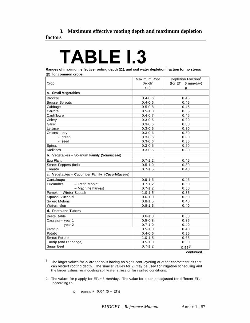
BUDGET – Reference Manual Annex 1. 67
3. Maximum effective rooting depth and maximum depletion factors
Ranges of maximum effective rooting depth (Zr), and soil water depletion fraction for no stress (p), for common crops Crop
Maximum Root Depth1
(m)
Depletion Fraction2 (for ET _ 5 mm/day)
p a. Small Vegetables Broccoli 0.4-0.6 0.45 Brussel Sprouts 0.4-0.6 0.45 Cabbage 0.5-0.8 0.45 Carrots 0.5-1.0 0.35 Cauliflower 0.4-0.7 0.45 Celery 0.3-0.5 0.20 Garlic 0.3-0.5 0.30 Lettuce 0.3-0.5 0.30 Onions - dry 0.3-0.6 0.30 - green 0.3-0.6 0.30 - seed 0.3-0.6 0.35 Spinach 0.3-0.5 0.20 Radishes 0.3-0.5 0.30 b. Vegetables – Solanum Family (Solanaceae) Egg Plant 0.7-1.2 0.45 Sweet Peppers (bell) 0.5-1.0 0.30 Tomato 0.7-1.5 0.40 c. Vegetables – Cucumber Family (Cucurbitaceae) Cantaloupe 0.9-1.5 0.45 Cucumber – Fresh Market 0.7-1.2 0.50 – Machine harvest 0.7-1.2 0.50 Pumpkin, Winter Squash 1.0-1.5 0.35 Squash, Zucchini 0.6-1.0 0.50 Sweet Melons 0.8-1.5 0.40 Watermelon 0.8-1.5 0.40 d. Roots and Tubers
Beets, table 0.6-1.0 0.50 Cassava – year 1 0.5-0.8 0.35 – year 2 0.7-1.0 0.40 Parsnip 0.5-1.0 0.40 Potato 0.4-0.6 0.35 Sweet Potato 1.0-1.5 0.65 Turnip (and Rutabaga) 0.5-1.0 0.50 Sugar Beet 0.7-1.2 0.553
continued…
1 The larger values for Zr are for soils having no significant layering or other characteristics that can restrict rooting depth. The smaller values for Zr may be used for irrigation scheduling and the larger values for modeling soil water stress or for rainfed conditions.
2 The values for p apply for ETc ≈ 5 mm/day. The value for p can be adjusted for different ETc
according to p = ptable 22 + 0.04 (5 – ETc)

BUDGET – Reference Manual Annex 1. 68
where p is expressed as a fraction and ETc as mm/day. 3 Sugar beets often experience late afternoon wilting in arid climates even at p < 0.55, with
usually only minor impact on sugar yield.
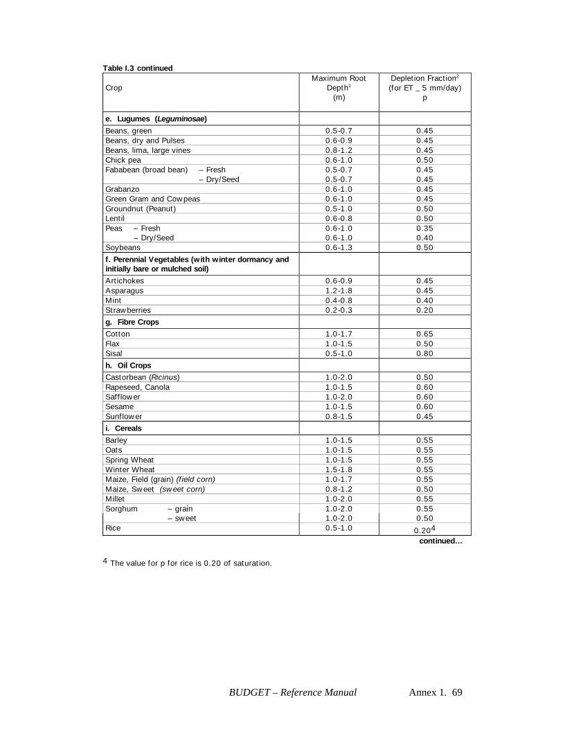
BUDGET – Reference Manual Annex 1. 69
Table I.3 continued Crop
Maximum Root Depth1
(m)
Depletion Fraction2 (for ET _ 5 mm/day)
p
e. Lugumes (Leguminosae) Beans, green 0.5-0.7 0.45 Beans, dry and Pulses 0.6-0.9 0.45 Beans, lima, large vines 0.8-1.2 0.45 Chick pea 0.6-1.0 0.50 Fababean (broad bean) – Fresh 0.5-0.7 0.45 – Dry/Seed 0.5-0.7 0.45 Grabanzo 0.6-1.0 0.45 Green Gram and Cowpeas 0.6-1.0 0.45 Groundnut (Peanut) 0.5-1.0 0.50 Lentil 0.6-0.8 0.50 Peas – Fresh 0.6-1.0 0.35 – Dry/Seed 0.6-1.0 0.40 Soybeans 0.6-1.3 0.50 f. Perennial Vegetables (with winter dormancy and initially bare or mulched soil)
Artichokes 0.6-0.9 0.45 Asparagus 1.2-1.8 0.45 Mint 0.4-0.8 0.40 Strawberries 0.2-0.3 0.20 g. Fibre Crops Cotton 1.0-1.7 0.65 Flax 1.0-1.5 0.50 Sisal 0.5-1.0 0.80 h. Oil Crops Castorbean (Ricinus) 1.0-2.0 0.50 Rapeseed, Canola 1.0-1.5 0.60 Safflower 1.0-2.0 0.60 Sesame 1.0-1.5 0.60 Sunflower 0.8-1.5 0.45 i. Cereals Barley 1.0-1.5 0.55 Oats 1.0-1.5 0.55 Spring Wheat 1.0-1.5 0.55
Winter Wheat 1.5-1.8 0.55
Maize, Field (grain) (field corn) 1.0-1.7 0.55 Maize, Sweet (sweet corn) 0.8-1.2 0.50 Millet 1.0-2.0 0.55 Sorghum – grain 1.0-2.0 0.55 – sweet 1.0-2.0 0.50 Rice 0.5-1.0 0.204
continued… 4 The value for p for rice is 0.20 of saturation.
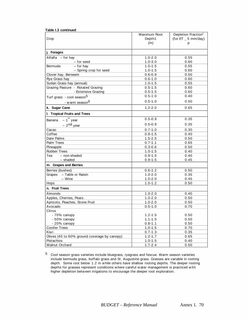
BUDGET – Reference Manual Annex 1. 70
Table I.3 continued Crop
Maximum Root Depth1
(m)
Depletion Fraction2 (for ET _ 5 mm/day)
p
j. Forages Alfalfa – for hay 1.0-2.0 0.55 – for seed 1.0-3.0 0.60 Bermuda – for hay 1.0-1.5 0.55 – Spring crop for seed 1.0-1.5 0.60 Clover hay, Berseem 0.6-0.9 0.50 Rye Grass hay 0.6-1.0 0.60 Sudan Grass hay (annual) 1.0-1.5 0.55 Grazing Pasture - Rotated Grazing 0.5-1.5 0.60 - Extensive Grazing 0.5-1.5 0.60
Turf grass - cool season5 0.5-1.0 0.40
- warm season5 0.5-1.0 0.50
k. Sugar Cane 1.2-2.0 0.65
l. Tropical Fruits and Trees
Banana – 1st year 0.5-0.9 0.35
– 2nd year 0.5-0.9 0.35
Cacao 0.7-1.0 0.30 Coffee 0.9-1.5 0.40 Date Palms 1.5-2.5 0.50 Palm Trees 0.7-1.1 0.65 Pineapple 0.3-0.6 0.50 Rubber Trees 1.0-1.5 0.40 Tea – non-shaded 0.9-1.5 0.40 – shaded 0.9-1.5 0.45 m. Grapes and Berries Berries (bushes) 0.6-1.2 0.50 Grapes – Table or Raisin 1.0-2.0 0.35 – Wine 1.0-2.0 0.45 Hops 1.0-1.2 0.50 n. Fruit Trees Almonds 1.0-2.0 0.40 Apples, Cherries, Pears 1.0-2.0 0.50 Apricots, Peaches, Stone Fruit 1.0-2.0 0.50 Avocado 0.5-1.0 0.70 Citrus - 70% canopy 1.2-1.5 0.50 - 50% canopy 1.1-1.5 0.50 - 20% canopy 0.8-1.1 0.50 Conifer Trees 1.0-1.5 0.70 Kiwi 0.7-1.3 0.35 Olives (40 to 60% ground coverage by canopy) 1.2-1.7 0.65 Pistachios 1.0-1.5 0.40 Walnut Orchard 1.7-2.4 0.50
5 Cool season grass varieties include bluegrass, ryegrass and fescue. Warm season varieties
include bermuda grass, buffalo grass and St. Augustine grass. Grasses are variable in rooting depth. Some root below 1.2 m while others have shallow rooting depths. The deeper rooting depths for grasses represent conditions where careful water management is practiced with higher depletion between irrigations to encourage the deeper root exploration.
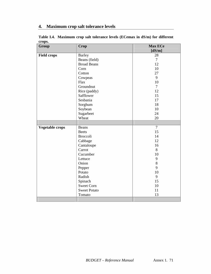
BUDGET – Reference Manual Annex 1. 71
4. Maximum crop salt tolerance levels Table I.4. Maximum crop salt tolerance levels (ECemax in dS/m) for different crops. Group Crop Max ECe
[dS/m] Field crops Barley
Beans (field) Broad Beans Corn Cotton Cowpeas Flax Groundnut Rice (paddy) Safflower Sesbania Sorghum Soybean Sugarbeet Wheat
28 7
12 10 27 9
10 7
12 15 17 18 10 24 20
Vegetable crops Beans
Beets Broccoli Cabbage Cantaloupe Carrot Cucumber Lettuce Onion Pepper Potato Radish Spinach Sweet Corn Sweet Potato Tomato
7 15 14 12 16 8
10 9 8 9
10 9
15 10 11 13
BUDGET – Reference Manual Annex 1. 72
Table I.4. Continued Group Crop Max ECe
[dS/m] Forage crops Alfalfa
Barley hay Bermuda grass Clover, Berseem Corn (forage) Harding grass Orchard grass Perennial rye Soudan grass Tall fescue Tall wheat grass Trefoil, big Trefoil, small Wheat grass
16 20 23 19 16 18 18 19 26 23 32 8
15 22
Fruit crops Almond
Apple, Pear Apricot Avocado Date palm Fig, Olive, Pomegranate Grape Grapefruit Lemon Orange Peach Plum Strawberry Walnut
7 8 6 6
32 14 12 8 8 8 7 7 4 8
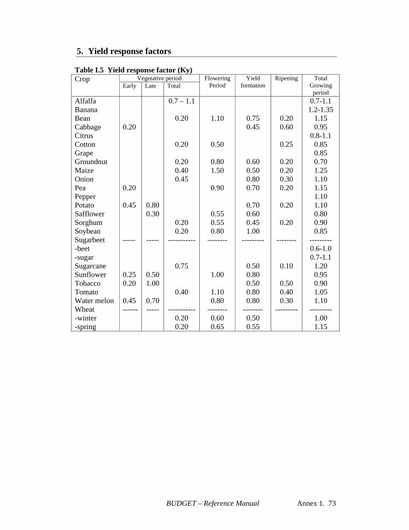
BUDGET – Reference Manual Annex 1. 73
5. Yield response factors
Table I.5 Yield response factor (Ky) Vegetative period Crop
Early Late Total Flowering
Period Yield
formation Ripening Total
Growing period
Alfalfa Banana Bean Cabbage Citrus Cotton Grape Groundnut Maize Onion Pea Pepper Potato Safflower Sorghum Soybean Sugarbeet -beet -sugar Sugarcane Sunflower Tobacco Tomato Water melon Wheat -winter -spring
0.20 0.20 0.45 ----- 0.25 0.20 0.45 ------
0.80 0.30
-----
0.50 1.00
0.70 -----
0.7 – 1.1
0.20
0.20
0.20 0.40 0.45
0.20 0.20
-----------
0.75
0.40
----------- 0.20 0.20
1.10
0.50
0.80 1.50
0.90
0.55 0.55 0.80
--------
1.00
1.10 0.80
-------- 0.60 0.65
0.75 0.45
0.60 0.50 0.80 0.70
0.70 0.60 0.45 1.00
---------
0.50 0.80 0.50 0.80 0.80
-------- 0.50 0.55
0.20 0.60
0.25
0.20 0.20 0.30 0.20
0.20
0.20
--------
0.10
0.50 0.40 0.30
---------
0.7-1.1 1.2-1.35
1.15 0.95
0.8-1.1 0.85 0.85 0.70 1.25 1.10 1.15 1.10 1.10 0.80 0.90 0.85
--------- 0.6-1.0 0.7-1.1
1.20 0.95 0.90 1.05 1.10
--------- 1.00 1.15
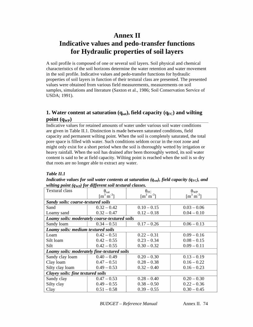
BUDGET – Reference Manual Annex II. 74
Annex II Indicative values and pedo-transfer functions
for Hydraulic properties of soil layers A soil profile is composed of one or several soil layers. Soil physical and chemical characteristics of the soil horizons determine the water retention and water movement in the soil profile. Indicative values and pedo-transfer functions for hydraulic properties of soil layers in function of their textural class are presented. The presented values were obtained from various field measurements, measurements on soil samples, simulations and literature (Saxton et al., 1986; Soil Conservation Service of USDA; 1991). 1. Water content at saturation (θsat), field capacity (θFC) and wilting point (θWP) Indicative values for retained amounts of water under various soil water conditions are given in Table II.1. Distinction is made between saturated conditions, field capacity and permanent wilting point. When the soil is completely saturated, the total pore space is filled with water. Such conditions seldom occur in the root zone and might only exist for a short period when the soil is thoroughly wetted by irrigation or heavy rainfall. When the soil has drained after been thoroughly wetted, its soil water content is said to be at field capacity. Wilting point is reached when the soil is so dry that roots are no longer able to extract any water. Table II.1 Indicative values for soil water contents at saturation (θsat), field capacity (θFC), and wilting point (θWP) for different soil textural classes. Textural class θsat
[m3 m-3] θFC
[m3 m-3] θWP
[m3 m-3] Sandy soils: coarse-textured soils Sand Loamy sand
0.32 – 0.42 0.32 – 0.47
0.10 – 0.15 0.12 – 0.18
0.03 – 0.06 0.04 – 0.10
Loamy soils: moderately coarse-textured soils Sandy loam 0.34 – 0.51 0.17 – 0.26 0.06 – 0.13 Loamy soils: medium textured soils Loam Silt loam Silt
0.42 – 0.51 0.42 – 0.55 0.42 – 0.55
0.22 – 0.31 0.23 – 0.34 0.30 – 0.32
0.09 – 0.16 0.08 – 0.15 0.09 – 0.11
Loamy soils: moderately fine-textured soils Sandy clay loam Clay loam Silty clay loam
0.40 – 0.49 0.47 – 0.51 0.49 – 0.53
0.20 – 0.30 0.28 – 0.38 0.32 – 0.40
0.13 – 0.19 0.16 – 0.22 0.16 – 0.23
Clayey soils: fine textured soils Sandy clay Silty clay Clay
0.47 – 0.53 0.49 – 0.55 0.51 – 0.58
0.28 – 0.40 0.38 – 0.50 0.39 – 0.55
0.20 – 0.30 0.22 – 0.36 0.30 – 0.45
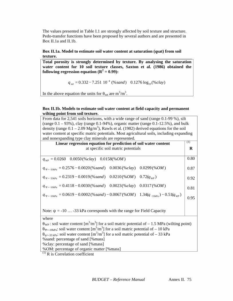
BUDGET – Reference Manual Annex II. 75
The values presented in Table I.1 are strongly affected by soil texture and structure. Pedo-transfer functions have been proposed by several authors and are presented in Box II.1a and II.1b. Box II.1a. Model to estimate soil water content at saturation (θsat) from soil texture. Total porosity is strongly determined by texture. By analysing the saturation water content for 10 soil texture classes, Saxton et al. (1986) obtained the following regression equation (R2 = 0.99):
)(%log1276.0)(%10251.7332.0 104 claysandsat +−= −θ
In the above equation the units for θsat are m3/m3. Box II.1b. Models to estimate soil water content at field capacity and permanent wilting point from soil texture. From data for 2,541 soils horizons, with a wide range of sand (range 0.1-99 %), silt (range 0.1 – 93%), clay (range 0.1-94%), organic matter (range 0.1-12.5%), and bulk density (range 0.1 – 2.09 Mg/m3), Rawls et al. (1982) derived equations for the soil water content at specific matric potentials. Most agricultural soils, including expanding and nonexpanding type clay minerals are represented.
Linear regression equation for prediction of soil water content at specific soil matric potentials
(1)
R
)(%0158.0)(%0050.00260.0 OMclayWP ++=θ
)(%0299.0)(%0036.0)(%0020.02576.033 OMclaysandkPa ++−=−=Ψθ
)(72.0)(%0210.0)(%0019.02319.033 WPkPa OMsand θθ ++−=−=Ψ
)(%0317.0)(%0023.0)(%0030.04118.010 OMclaysandkPa ++−=−=Ψθ
)(51.0)(34.1)(%0067.0)(%0002.00619.0 3310 WPkPakPa OMsand θθθ −+−−= −−=Ψ
Note: ψ = -10 … -33 kPa corresponds with the range for Field Capacity
0.80
0.87
0.92
0.81
0.95
where θWP : soil water content [m3/m3] for a soil matric potential of – 1.5 MPa (wilting point) θΨ=-10kPa: soil water content [m3/m3] for a soil matric potential of – 10 kPa θψ=-33 kPa: soil water content [m3/m3] for a soil matric potential of – 33 kPa %sand: percentage of sand [%mass] %clay: percentage of sand [%mass] %OM: percentage of organic matter [%mass] (1) R is Correlation coefficient
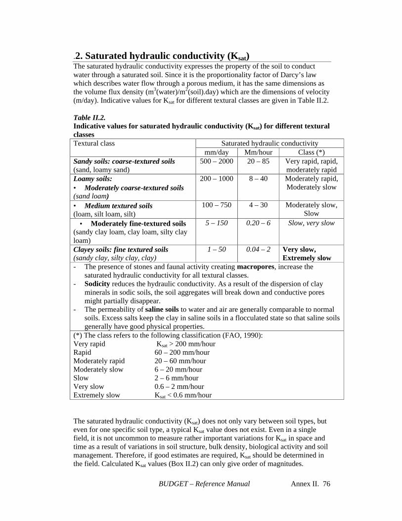
BUDGET – Reference Manual Annex II. 76
.2. Saturated hydraulic conductivity (Ksat) The saturated hydraulic conductivity expresses the property of the soil to conduct water through a saturated soil. Since it is the proportionality factor of Darcy’s law which describes water flow through a porous medium, it has the same dimensions as the volume flux density (m3(water)/m2(soil).day) which are the dimensions of velocity (m/day). Indicative values for Ksat for different textural classes are given in Table II.2. Table II.2. Indicative values for saturated hydraulic conductivity (Ksat) for different textural classes
Saturated hydraulic conductivity Textural class mm/day Mm/hour Class (*)
Sandy soils: coarse-textured soils (sand, loamy sand)
500 – 2000 20 – 85 Very rapid, rapid, moderately rapid
Loamy soils: • Moderately coarse-textured soils (sand loam)
200 – 1000 8 – 40 Moderately rapid, Moderately slow
• Medium textured soils (loam, silt loam, silt)
100 – 750 4 – 30 Moderately slow, Slow
• Moderately fine-textured soils (sandy clay loam, clay loam, silty clay loam)
5 – 150 0.20 – 6 Slow, very slow
Clayey soils: fine textured soils (sandy clay, silty clay, clay)
1 – 50 0.04 – 2 Very slow, Extremely slow
- The presence of stones and faunal activity creating macropores, increase the saturated hydraulic conductivity for all textural classes.
- Sodicity reduces the hydraulic conductivity. As a result of the dispersion of clay minerals in sodic soils, the soil aggregates will break down and conductive pores might partially disappear.
- The permeability of saline soils to water and air are generally comparable to normal soils. Excess salts keep the clay in saline soils in a flocculated state so that saline soils generally have good physical properties.
(*) The class refers to the following classification (FAO, 1990): Very rapid Rapid Moderately rapid Moderately slow Slow Very slow Extremely slow
Ksat > 200 mm/hour 60 – 200 mm/hour 20 – 60 mm/hour 6 – 20 mm/hour 2 – 6 mm/hour 0.6 – 2 mm/hour Ksat < 0.6 mm/hour
The saturated hydraulic conductivity (Ksat) does not only vary between soil types, but even for one specific soil type, a typical Ksat value does not exist. Even in a single field, it is not uncommon to measure rather important variations for Ksat in space and time as a result of variations in soil structure, bulk density, biological activity and soil management. Therefore, if good estimates are required, Ksat should be determined in the field. Calculated Ksat values (Box II.2) can only give order of magnitudes.
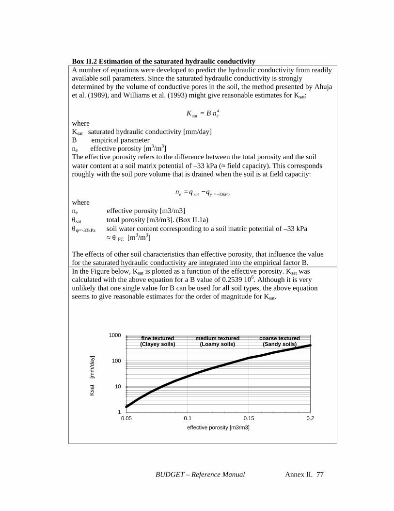
BUDGET – Reference Manual Annex II. 77
Box II.2 Estimation of the saturated hydraulic conductivity A number of equations were developed to predict the hydraulic conductivity from readily available soil parameters. Since the saturated hydraulic conductivity is strongly determined by the volume of conductive pores in the soil, the method presented by Ahuja et al. (1989), and Williams et al. (1993) might give reasonable estimates for Ksat:
4esat nBK =
where Ksat saturated hydraulic conductivity [mm/day] B empirical parameter ne effective porosity [m3/m3] The effective porosity refers to the difference between the total porosity and the soil water content at a soil matrix potential of –33 kPa (≈ field capacity). This corresponds roughly with the soil pore volume that is drained when the soil is at field capacity:
kPasaten 33−=−= ψθθ where ne effective porosity [m3/m3] θsat total porosity [m3/m3]. (Box II.1a) θψ=-33kPa soil water content corresponding to a soil matric potential of –33 kPa ≈ θ FC [m3/m3] The effects of other soil characteristics than effective porosity, that influence the value for the saturated hydraulic conductivity are integrated into the empirical factor B. In the Figure below, Ksat is plotted as a function of the effective porosity. Ksat was calculated with the above equation for a B value of 0.2539 106. Although it is very unlikely that one single value for B can be used for all soil types, the above equation seems to give reasonable estimates for the order of magnitude for Ksat.
0.05 0.1 0.15 0.2
effective porosity [m3/m3]
1
10
100
1000
Ksa
t [
mm
/day
]
coarse textured (Sandy soils)
medium textured(Loamy soils)
fine textured(Clayey soils)
BUDGET – Reference Manual Annex II. 78
3. Drainage characteristic (τ) To simulate the drainage inside and the percolation out of a soil layer, and to simulate the infiltration of rainfall and/or irrigation, BUDGET makes use of a drainage function:
11
)(−−
−=∆
∆−
−
FCsat
FCi
ee
t FCsati
θθ
θθ
θθτθ
Where ∆θi/∆t decrease in soil water content during time step [m3.m-3.day-1] τ drainage characteristic [-] θi actual soil water content [m3.m-3] θSAT soil water content at saturation [m3.m-3] θFC soil water content at field capacity [m3.m-3] ∆t time step [day] note: IF θi = θFC THAN ∆θi/∆t = 0 IF θi = θSAT THAN ∆θi/∆t = τ (θSAT - θFC) The drainage function describes the amount of water lost by free drainage as a function of time for any moisture content between saturation and field capacity. When field capacity is reached further drainage of the soil layer is disregarded. A drainage function is described by the dimensionless drainage characteristic τ (tau) (see Chapter 3 Drainage subroutine). Indicative values for τ for different texture classes are presented in Table II.3. The values were derived from simulation runs whereby thick uniform soil layers of various textural compositions were allowed to drain after been saturated (Barrios Gonzales, 1999). The simulations were performed by means of an explanatory model (Vanclooster et al., 1994) that describes the water movement with the help of the Richard equation (Jury et al., 1991). To run the simulations the water retention curve (θ(h)) and hydraulic characteristic curve (K(h)) of the soil layers are required. For the various textural classes, several typical θ(h) relationship were described by the Van Genuchten equation (Van Genuchten et al., 1991). The corresponding K(h) relationships were derived by means of Gardner model from the θ(h) relationships and typical values for Ksat. On the basis of the obtained τ value, three different drainage groups can be distinguished. Soil layers belonging to Group I have more than 50% of sand and less than 20% of clay in their particle composition. The τ value within this group is always higher than 0.5 and even higher than 0.9 if the sand content exceeds 80%. Group II encompasses medium, moderately fine and fine textured soil layers. The textural composition varies from soil layers having 90% silt (silty soil) to soils with almost equal proportions of clay and sand and almost no silt (sandy clay soil). The τ value is situated between 0.25 and 0.45. Group III represents the fine textured clay soils with low τ values (smaller than 0.25) to very low τ values (about 0.10) for soil layers with more than 60% clay. Indicative values for τ can also be derived from Fig. II.3.
BUDGET – Reference Manual Annex II. 79
Table II.3 Indicative values for the drainage characteristic (τ) of soil layers for different textural classes. Textural class Drainage characteristic (τ) Drainage group Sandy soils: coarse-textured soils Sand Loamy sand
1 – 0.9 0.85 – 0.65
I I
Loamy soils: moderately coarse-textured soils Sandy loam 0.65 – 0.50 I Loamy soils: medium textured soils Loam Silt loam Silt
0.45 – 0.35 0.45 – 0.35 0.45 – 0.35
II II II
Loamy soils: moderately fine-textured soils Sandy clay loam Clay loam Silty clay loam
0.40 – 0.25 0.40 – 0.25 0.40 – 0.25
II II II
Clayey soils: fine textured soils Sandy clay Silty clay Clay
0.40 – 0.25 0.40 – 0.25 0.25 – 0.10
II II III
The close relationship (Fig. II.3) between the dimensionless drainage characteristics (ι) and the hydraulic conductivity at saturation (Ksat) is given by
10866.00 )(log8063.0 10 ≤=≤ Ksateτ where Ksat is given in mm/day.
1 10 100 1000
Saturated hydraulic conductivity (mm/day)
0
0.2
0.4
0.6
0.8
1
drai
nage
cha
ract
eris
tic (
tau)
Figure II.3 Indicative values for the drainage characteristic (tau)
for various values of saturated hydraulic conductivity (Ksat)
Related Documents


