A Software Effort Estimation as a Multi-objective Learning Problem Leandro L. Minku and Xin Yao, The University of Birmingham Ensembles of learning machines are promising for software effort estimation (SEE), but need to be tailored for this task to have their potential exploited. A key issue when creating ensembles is to produce diverse and accurate base models. Depending on how differently different performance measures behave for SEE, they could be used as a natural way of creating SEE ensembles. We propose to view SEE model creation as a multi-objective learning problem. A multi-objective evolutionary algorithm (MOEA) is used to better understand the trade-off among different performance measures by creating SEE models through the simul- taneous optimisation of these measures. We show that the performance measures behave very differently, presenting sometimes even opposite trends. They are then used as a source of diversity for creating SEE ensembles. A good trade-off among different measures can be obtained by using an ensemble of MOEA so- lutions. This ensemble performs similarly or better than a model that does not consider these measures explicitly. Besides, MOEA is also flexible, allowing emphasis of a particular measure if desired. In conclu- sion, MOEA can be used to better understand the relationship among performance measures and has shown to be very effective in creating SEE models. Categories and Subject Descriptors: D.2.9 [Software Engineering]: Management—Cost estimation; I.2.6 [Artificial Intelligence]: Learning—Connectionism and Neural Nets; Concept Learning; I.2.8 [Artificial Intelligence]: Problem Solving, Control Methods, and Search General Terms: Experimentation, Algorithms, Management Additional Key Words and Phrases: Software effort estimation, ensembles of learning machines, multi- objective evolutionary algorithms ACM Reference Format: Minku, L., and Yao, X. 2011. Software Effort Estimation as a Multi-objective Learning Problem. ACM Trans. Softw. Eng. Methodol. V, N, Article A (January YYYY), 32 pages. DOI = 10.1145/0000000.0000000 http://doi.acm.org/10.1145/0000000.0000000 1. INTRODUCTION Estimating the cost of a software project is a task of strategic importance in project management. Both over and underestimations of cost can cause serious problems to a company. For instance, overestimations may result in a company losing contracts or wasting resources, whereas underestimations may result in poor quality, delayed or unfinished softwares. The major contributing factor for software cost is effort [Agarwal et al. 2001]. This work is supported by two EPSRC grants (Nos. EP/D052785/1 and EP/J017515/1). Authors’ address: L. Minku and X. Yao are with the Centre of Excellence for Research in Computational In- telligence and Applications, School of Computer Science, The University of Birmingham, Edgbaston, Birm- ingham, B15 2TT, UK. c ACM (2012). This is the author’s version of the work, which has been accepted for publication at ACM TOSEM. It is posted here by permission of ACM for your personal use. Not for redistribution. The definitive version will be published soon. Permission to make digital or hard copies of part or all of this work for personal or classroom use is granted without fee provided that copies are not made or distributed for profit or commercial advantage and that copies show this notice on the first page or initial screen of a display along with the full citation. Copyrights for components of this work owned by others than ACM must be honored. Abstracting with credit is per- mitted. To copy otherwise, to republish, to post on servers, to redistribute to lists, or to use any component of this work in other works requires prior specific permission and/or a fee. Permissions may be requested from Publications Dept., ACM, Inc., 2 Penn Plaza, Suite 701, New York, NY 10121-0701 USA, fax +1 (212) 869-0481, or [email protected]. c YYYY ACM 1049-331X/YYYY/01-ARTA $15.00 DOI 10.1145/0000000.0000000 http://doi.acm.org/10.1145/0000000.0000000 ACM Transactions on Software Engineering and Methodology, Vol. V, No. N, Article A, Pub. date: January YYYY.

Welcome message from author
This document is posted to help you gain knowledge. Please leave a comment to let me know what you think about it! Share it to your friends and learn new things together.
Transcript

A
Software Effort Estimation as a Multi-objective Learning Problem
Leandro L. Minku and Xin Yao, The University of Birmingham
Ensembles of learning machines are promising for software effort estimation (SEE), but need to be tailoredfor this task to have their potential exploited. A key issue when creating ensembles is to produce diverseand accurate base models. Depending on how differently different performance measures behave for SEE,they could be used as a natural way of creating SEE ensembles. We propose to view SEE model creationas a multi-objective learning problem. A multi-objective evolutionary algorithm (MOEA) is used to betterunderstand the trade-off among different performance measures by creating SEE models through the simul-taneous optimisation of these measures. We show that the performance measures behave very differently,presenting sometimes even opposite trends. They are then used as a source of diversity for creating SEEensembles. A good trade-off among different measures can be obtained by using an ensemble of MOEA so-lutions. This ensemble performs similarly or better than a model that does not consider these measuresexplicitly. Besides, MOEA is also flexible, allowing emphasis of a particular measure if desired. In conclu-sion, MOEA can be used to better understand the relationship among performance measures and has shownto be very effective in creating SEE models.
Categories and Subject Descriptors: D.2.9 [Software Engineering]: Management—Cost estimation; I.2.6[Artificial Intelligence]: Learning—Connectionism and Neural Nets; Concept Learning; I.2.8 [Artificial
Intelligence]: Problem Solving, Control Methods, and Search
General Terms: Experimentation, Algorithms, Management
Additional Key Words and Phrases: Software effort estimation, ensembles of learning machines, multi-objective evolutionary algorithms
ACM Reference Format:
Minku, L., and Yao, X. 2011. Software Effort Estimation as a Multi-objective Learning Problem. ACM Trans.Softw. Eng. Methodol. V, N, Article A (January YYYY), 32 pages.DOI = 10.1145/0000000.0000000 http://doi.acm.org/10.1145/0000000.0000000
1. INTRODUCTION
Estimating the cost of a software project is a task of strategic importance in projectmanagement. Both over and underestimations of cost can cause serious problems toa company. For instance, overestimations may result in a company losing contractsor wasting resources, whereas underestimations may result in poor quality, delayed orunfinished softwares. The major contributing factor for software cost is effort [Agarwalet al. 2001].
This work is supported by two EPSRC grants (Nos. EP/D052785/1 and EP/J017515/1).Authors’ address: L. Minku and X. Yao are with the Centre of Excellence for Research in Computational In-telligence and Applications, School of Computer Science, The University of Birmingham, Edgbaston, Birm-ingham, B15 2TT, UK.c© ACM (2012). This is the author’s version of the work, which has been accepted for publication at ACM
TOSEM. It is posted here by permission of ACM for your personal use. Not for redistribution. The definitiveversion will be published soon.Permission to make digital or hard copies of part or all of this work for personal or classroom use is grantedwithout fee provided that copies are not made or distributed for profit or commercial advantage and thatcopies show this notice on the first page or initial screen of a display along with the full citation. Copyrightsfor components of this work owned by others than ACM must be honored. Abstracting with credit is per-mitted. To copy otherwise, to republish, to post on servers, to redistribute to lists, or to use any componentof this work in other works requires prior specific permission and/or a fee. Permissions may be requestedfrom Publications Dept., ACM, Inc., 2 Penn Plaza, Suite 701, New York, NY 10121-0701 USA, fax +1 (212)869-0481, or [email protected]© YYYY ACM 1049-331X/YYYY/01-ARTA $15.00
DOI 10.1145/0000000.0000000 http://doi.acm.org/10.1145/0000000.0000000
ACM Transactions on Software Engineering and Methodology, Vol. V, No. N, Article A, Pub. date: January YYYY.

A:2 L. Minku and X. Yao
Human made effort estimations tend to be strongly affected by effort-irrelevant andmisleading information [Jrgensen and Grimstad 2011]. Moreover, developers tend notto improve their effort estimation uncertainty assessment even after feedback abouttheir estimates is provided [Gruschke and Jørgensen 2008]. An alternative to humanmade effort estimations is to use automated effort estimators. Models for estimatingsoftware effort can be used as decision support tools, allowing investigation of theimpact of certain requirements and development team features on the cost/effort of aproject to be developed.
A major difficulty in performing software estimation is the lack of project data thatinclude size and detailed quantitative counts on the elements of UML models used,e.g., the number of analysis classes, number of relationship types, number of associ-ated attributes, use-case point, etc. As a result, even though UML models are com-monly used, it is still very difficult to do software estimation based on UML mod-els constructed in the early stage of software development. Hence, it is very difficultto further test, evaluate and enhance very promising estimation approaches that arebased on the UML models constructed in the early state of requirements analysis [Tanet al. 2009; Mohagheghi et al. 2005; Tan et al. 2006]. The analysis of the effectivenessof estimation models based on limited project data thus becomes an important fieldto be investigated. Different automated methods for software cost or Software EffortEstimation (SEE) have been proposed [Jorgensen and Shepperd 2007].
In the present work, we look into a type of machine learning method which has re-cently attracted attention from the SEE community [Braga et al. 2007; Kultur et al.2009; Kocaguneli et al. 2009; Minku and Yao 2011], namely ensembles of learning ma-chines. Ensembles are sets of learners trained to perform the same task and combinedwith the aim of improving predictive performance [Chen and Yao 2009]. When com-bining learning models in an attempt to get more accurate predictions, it is commonlyagreed that these base models should behave differently from each other. Otherwise,the overall prediction will not be better than the individual predictions [Brown et al.2005; L. I and Whitaker 2003]. This behaviour matches intuition: if models that makethe same mistakes are combined into an ensemble, the ensemble will make the samemistakes as the individual models and its performance will be no better than the in-dividual performances. On the contrary, ensembles composed of diverse models cancompensate the mistakes of certain models through the correct predictions performedby other models. So, diversity refers to the predictions/errors made by the models. Twomodels are said to be diverse if they make different errors on the same data points[Chandra and Yao 2006]. Different ensemble learning approaches can be seen as dif-ferent ways to generate diversity among the base models.
Even though ensembles have been shown to be promising for SEE, it is necessary totailor them for this estimation task. Simply using any general purpose ensemble ap-proach from the literature does not necessarily improve SEE in comparison to singlelearning machines [Minku and Yao 2011]. Minku and Yao [2012] showed that com-bining the power of ensembles to local learning through the use of bagging ensemblesof regression trees outperforms several other learning machines for SEE in terms ofMean Absolute Error (MAE). This combination is a way to tailor ensembles for SEE,but Minku and Yao [2012] also show that more improvements may still be achievedif additional tailoring is performed. Very recently, Kocaguneli et al. [2011] proposedan ensemble method claimed to outperform single learners for SEE. However, theirmethod is not fully automated, as it needs manual/visual inspection of extensive ex-periments to create the ensemble. Section 2 explains related work on machine learningand in particular ensembles for SEE.
Much of the SEE work involves empirical evaluation of models and several differentmeasures of performance can be used for that. Examples of measures are two popular
ACM Transactions on Software Engineering and Methodology, Vol. V, No. N, Article A, Pub. date: January YYYY.

Software Effort Estimation as a Multi-objective Learning Problem A:3
measures based on the magnitude of the relative error, namely Mean Magnitude of theRelative Error (MMRE) and percentage of estimations within N% of the actual value(PRED(N)), and a measure based on the logarithm of the residuals recommended byFoss et al. [2003], namely Logarithmic Standard Deviation (LSD). Different measurescan behave differently and it is highly unlikely that there is a “single, simple-to-use,universal goodness-of-fit kind of metric” [Foss et al. 2003], i.e., none of these measuresis totally free of problems.
The relationship among different measures is not yet well understood. For example,it is not known to what extent a lower MMRE could be related to a higher LSD and viceversa, or how different are the MMREs associated to the same PRED value. Dependingon how differently these performance measures behave, it may be possible to use themas a natural way to generate diversity in ensembles for SEE. With that in mind, thispaper aims at answering the following research questions:
— RQ1: What is the relationship among different performance measures for SEE?— RQ2: Can we use different performance measures as a source of diversity to cre-
ate SEE ensembles? In particular, can that improve the performance in comparisonto models created without considering these measures explicitly? Existing modelsdo not necessarily consider the performance measures in which we are interestedexplicitly. For example, Multi-layer Perceptrons (MLPs) are usually trained usingBackpropagation, which is based on the mean squared error. So, they can only im-prove MMRE, PRED and LSD indirectly. We would like to know whether creating anensemble considering MMRE, PRED and LSD explicitly leads to more improvementin the SEE context.
— RQ3: Is it possible to create models that emphasize particular performance mea-sures should we wish to do so? For example, if there is a certain measure that webelieve to be more appropriate than the others, can we create a model that particu-larly improves performance considering this measure? This is useful not only for thecase where the software manager has sufficient domain knowledge to chose a certainmeasure, but also (and mainly) if there are future developments of the SEE researchshowing that a certain measure is better than others for a certain purpose.
In order to answer these questions, we formulate the problem of creating SEE mod-els as a multi-objective learning problem that considers different performance mea-sures explicitly as objectives to be optimised. This formulation is key to answer theresearch questions because it allows us to use a Multi-objective Evolutionary Algo-rithm (MOEA) [Wang et al. 2010] to generate SEE models that are generally goodconsidering all the pre-defined performance measures. This feature allows us to useplots of the performances of these models to understand the relationship among theperformance measures and how differently they behave. Once these models are ob-tained, the models that perform best for each different performance measure can bedetermined. These models behave differently from each other and can be used to forma diverse ensemble that provides an ideal trade-off among these measures. Choosinga performance measure is not an easy task. By using our ensemble, the software man-ager does not need to chose a certain performance measure, as an ideal trade-off amongdifferent measures is provided. As an additional benefit of this approach, each of themodels that compose the ensemble can also be used separately to emphasize a spe-cific performance measure if desired. The performance measures used by the MOEAin this work are MMRE, PRED(25) and LSD. Section 3 explains MOEAs and section 4explains our proposed approach to use MOEAs for creating SEE models.
Our analysis shows that the different performance measures behave very differentlywhen analysed at their individual best level and sometimes present even opposite be-haviour (RQ1). For example, when considering nondominated (section 3) solutions, as
ACM Transactions on Software Engineering and Methodology, Vol. V, No. N, Article A, Pub. date: January YYYY.
A:4 L. Minku and X. Yao
MMRE is improved, LSD tends to get worse. This is an indicator that these mea-sures can be used to create diverse ensembles for SEE. We then show that MOEA issuccessful in generating SEE ensemble models by optimising different performancemeasures explicitly at the same time (RQ2). The ensembles are composed of nondomi-nated solutions selected from the last generation of the MOEA, as explained in section4. These ensembles present performance similar or better than a model that does notoptimize the three measures concurrently. Furthermore, the similar or better perfor-mance is achieved considering all the measures used to create the ensemble, showingthat these ensembles not only provide a better trade-off among different measures, butalso improve the performance considering these measures. We also show that MOEAis flexible, allowing us to chose solutions which emphasize certain measures, if desired(RQ3).
The base learners generated by the MOEA in this work are Multi-layer Perceptrons(MLPs) [Bishop 2005], which have been showing success in the SEE literature for notbeing restricted to linear project data [Tronto et al. 2007]. Even though we generateMLPs in this work, MOEAs could also be used to generate other types of base learn-ers, such as RBFs, RTs and linear regression equations. An additional comparison ofMOEA to evolve MLPs was performed against nine other types of models. The com-parison shows that the MOEA-evolved MLPs were ranked first more often in terms offive different performance measures, but performed less well in terms of LSD. Theywere also ranked first more often for the data sets likely to be more heterogeneous. Itis important to note, though, that this additional comparison is not only evaluating theMOEA and the multi-objective formulation of the problem, but also the type of modelbeing evolved (MLP). Other types of models could also be evolved by the MOEA andcould possibly provide better results in terms of LSD. As the key point of this paper isto analyse the multi-objective formulation of the creation of SEE models, and not thecomparison among different types of models, the experimentation with different typesof MOEA and different types of base models is left as future work.
This paper is organised as follows. Section 2 presents related work on machine learn-ing and ensembles for SEE. Section 3 explains MOEAs and the type of MOEA used inthis work. Section 4 explains our approach for creating SEE models (including ensem-bles) through MOEAs. In particular, section 4.1 explains the multi-objective formula-tion of the problem of creating SEE models. Section 5 explains the experimental setupfor answering the research questions and evaluating our approach. Section 6 explainsthe data sets used in the experiment. Section 7 provides an analysis of the relation-ship among different performance measures (RQ1). Section 8 provides an evaluationof the MOEA’s ability of creating ensembles by optimising several different measuresat the same time (RQ2). Section 9 shows that MOEAs are flexible, allowing us to cre-ate models that emphasize particular performance measures, if desired (RQ3). Section10 shows that there is still room for improvement in the choice of MOEA models tobe used for SEE. Section 11 complements the evaluation by checking how well thePareto ensemble of MLPs performs in comparison to other types of models. Section 12presents the conclusions and future work.
2. MACHINE LEARNING FOR SEE
Several different methods for automating software cost/effort estimation have beenproposed [Jorgensen and Shepperd 2007]. For example, Shepperd and Schofield [1997]present a landmark study using estimation by analogy, which is a type of case-basedreasoning. The features and effort of completed projects are stored and then the effortestimation problem is regarded as the one of finding the most similar projects in termsof Euclidean distance to the one for which an estimation is required. The approachwas evaluated on nine data sets and obtained in general better MMRE and PRED(25)
ACM Transactions on Software Engineering and Methodology, Vol. V, No. N, Article A, Pub. date: January YYYY.
Software Effort Estimation as a Multi-objective Learning Problem A:5
than more traditional stepwise regression models. Chulani et al. [1999] presented an-other study using a Bayesian approach to combine a priori information based on ex-pert knowledge to a linear regression model based on log transformation of the data.The proposed approach outperforms linear regression models based on log transformeddata in terms of PRED(20), PRED(25) and PRED(30) on one data set and its extendedversion. No comparison with Shepperd and Schofield [1997]’s work was given.
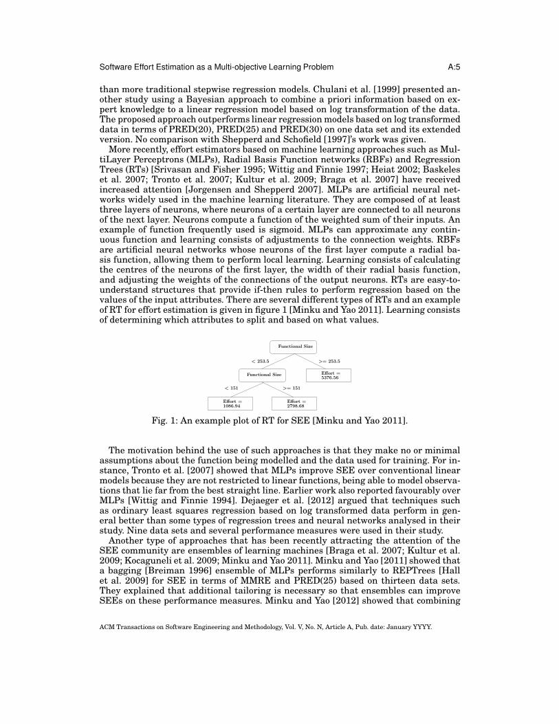
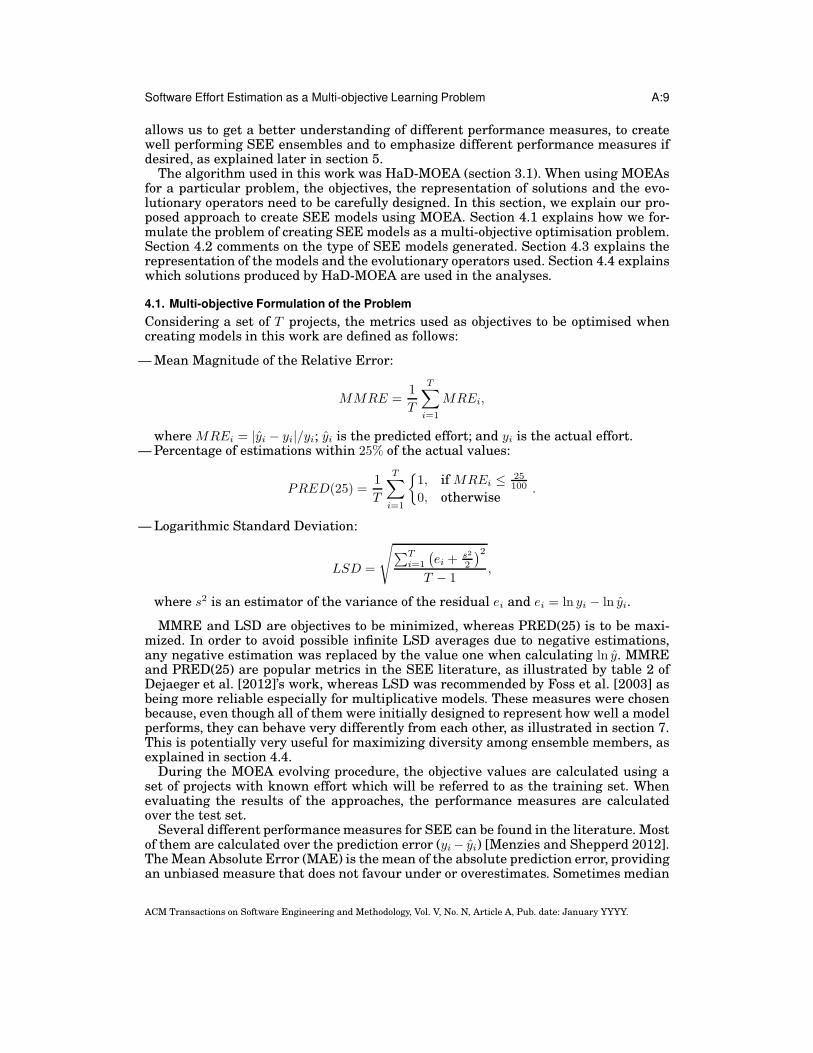
More recently, effort estimators based on machine learning approaches such as Mul-tiLayer Perceptrons (MLPs), Radial Basis Function networks (RBFs) and RegressionTrees (RTs) [Srivasan and Fisher 1995; Wittig and Finnie 1997; Heiat 2002; Baskeleset al. 2007; Tronto et al. 2007; Kultur et al. 2009; Braga et al. 2007] have receivedincreased attention [Jorgensen and Shepperd 2007]. MLPs are artificial neural net-works widely used in the machine learning literature. They are composed of at leastthree layers of neurons, where neurons of a certain layer are connected to all neuronsof the next layer. Neurons compute a function of the weighted sum of their inputs. Anexample of function frequently used is sigmoid. MLPs can approximate any contin-uous function and learning consists of adjustments to the connection weights. RBFsare artificial neural networks whose neurons of the first layer compute a radial ba-sis function, allowing them to perform local learning. Learning consists of calculatingthe centres of the neurons of the first layer, the width of their radial basis function,and adjusting the weights of the connections of the output neurons. RTs are easy-to-understand structures that provide if-then rules to perform regression based on thevalues of the input attributes. There are several different types of RTs and an exampleof RT for effort estimation is given in figure 1 [Minku and Yao 2011]. Learning consistsof determining which attributes to split and based on what values.
1086.94
>= 253.5
< 151 >= 151
< 253.5
Functional Size
Functional Size Effort =
5376.56
Effort =
2798.68
Effort =
Fig. 1: An example plot of RT for SEE [Minku and Yao 2011].
The motivation behind the use of such approaches is that they make no or minimalassumptions about the function being modelled and the data used for training. For in-stance, Tronto et al. [2007] showed that MLPs improve SEE over conventional linearmodels because they are not restricted to linear functions, being able to model observa-tions that lie far from the best straight line. Earlier work also reported favourably overMLPs [Wittig and Finnie 1994]. Dejaeger et al. [2012] argued that techniques suchas ordinary least squares regression based on log transformed data perform in gen-eral better than some types of regression trees and neural networks analysed in theirstudy. Nine data sets and several performance measures were used in their study.
Another type of approaches that has been recently attracting the attention of theSEE community are ensembles of learning machines [Braga et al. 2007; Kultur et al.2009; Kocaguneli et al. 2009; Minku and Yao 2011]. Minku and Yao [2011] showed thata bagging [Breiman 1996] ensemble of MLPs performs similarly to REPTrees [Hallet al. 2009] for SEE in terms of MMRE and PRED(25) based on thirteen data sets.They explained that additional tailoring is necessary so that ensembles can improveSEEs on these performance measures. Minku and Yao [2012] showed that combining
ACM Transactions on Software Engineering and Methodology, Vol. V, No. N, Article A, Pub. date: January YYYY.

A:6 L. Minku and X. Yao
the power of ensembles to local learning through the use of bagging ensembles of REP-Trees outperforms several other learning machines for SEE in terms of MAE. Combin-ing ensembles and locality is a way to tailor ensembles for SEE, but Minku and Yao[2012] also show that more improvements may still be achieved if additional tailoringis performed. Kocaguneli et al. [2011] proposed an ensemble method that outperformssingle learners for SEE. Their method combines several types of so called solo-methods(combinations of single learners and preprocessing techniques) to perform SEE. Theyreported that the ensemble presents less instability than solo-methods when rankedin terms of the total number of wins, losses and wins − losses considering severaldifferent performance measures and twenty data sets. These observations confirmedearlier results reported in the ensemble learning literature that ensembles generallyperform better than its component learners. They also reported that the ensemblesobtained less losses than other methods. As an additional contribution, their extensivestudy showed that the non-linear approaches CART (a type of RT) and estimation byanalogy based on log transformed data can outperform other methods such as linearregression based on log transformed data.
However, their approach [Kocaguneli et al. 2011] has high implementation complex-ity and is not fully automated. It requires an extensive experimentation procedureusing several types of single learners and preprocessing techniques for creating theensemble. It consists of selecting the “best” solo-methods in terms of losses and sta-bility to compose the ensemble, by manually/visually checking and comparing theirstability. The manual/visual checking process is needed because it is necessary notonly to determine what solo-methods have the lowest number of losses (that by itselfcould be automated), but also to check whether these are the same as the ones compar-atively more stable and what level of stability should be considered as comparativelysuperior or not.
Differently from Kocaguneli et al. [2011]’s approach, our approach is fully auto-mated. Once developed, a tool using our MOEA can be easily run to learn a modelthat uses data from a specific company. It is worth noting that parameters choice ofour approach can be automated, as long as the developer of the tool embeds on it sev-eral different parameter values to be tested on a certain percentage of the completedprojects of the company. More importantly, we can create ensembles in such a way toencourage both accuracy and diversity, which is known to be beneficial for ensembles[Brown et al. 2005; L. I and Whitaker 2003]. Kocaguneli et al. [2011]’s approach ismainly focused on accuracy, providing no guarantee that the base learners performdiversely. As explained by Chandra and Yao [2006], ensembles need their base modelsto be both accurate and diverse in order to perform well. However, there is a trade-offbetween accuracy and diversity of base models. So, if we focus only on improving theiraccuracy, they are likely to lack diversity, reducing the accuracy of the ensemble as awhole.
3. MOEAS
MOEAs are population-based optimisation algorithms that evolve sets of candidate so-lutions by optimising two or more possibly conflicting objectives. Candidate solutionsare generated/evolved through evolutionary operators such as crossover and mutationin rounds called generations. The evolutionary process is frequently guided by the con-cept of dominance, which is defined as follows. Consider a multi-objective optimisationproblem consisting of N objectives fi(x) to be minimized, where x is a p dimensionalvector containing p design or decision variables [Srinivas and Deb 1994]. A solutionx(1) dominates a solution x(2) iff:
ACM Transactions on Software Engineering and Methodology, Vol. V, No. N, Article A, Pub. date: January YYYY.
Software Effort Estimation as a Multi-objective Learning Problem A:7
fi(x(1)) ≤ fi(x
(2)) ∀i ∧ ∃i | fi(x(1)) < fi(x
(2))
This concept can easily be generalized to problems involving maximization.The set of optimal solutions (nondominated by any other solution) is called Pareto
front. Even though the true Pareto front is very difficult to be found, a MOEA can find aset of acceptable solutions nondominated by any other solution in the last generation.We will refer to these solutions as Pareto solutions.
There exist several different MOEAs. As examples we can cite the conventional andwell known Nondominated Sorting Genetic Algorithm II (NSGA-II) [Deb et al. 2002];the improved Strength Pareto Evolutionary Algorithm (SPEA2) [Zitzler et al. 2002];the two-archive algorithm [Praditwong and Yao 2006], which has been used in the soft-ware engineering context for software module clustering by Praditwong et al. [2011];and the Harmonic Distance MOEA (HaD-MOEA) [Wang et al. 2010].
Once a representation, evolutionary operators and objective functions are defined,our proposed approach can be used in combination to any MOEA. We chose HaD-MOEA as the algorithm to be used in our experiments due to its simplicity and advan-tages over NSGA-II as explained in section 3.1. This paper does not intend to show thata particular MOEA performs better or worse than another. For that reason, we leavethe evaluation of other MOEAs to evolve SEE models as future work. In the currentpaper, we concentrate on the multi-objective formulation of the problem, how to use amulti-objective approach to solve it, and to provide a better understanding of differentperformance measures.
3.1. HaD-MOEA
HaD-MOEA [Wang et al. 2010] is a MOEA that improves upon NSGA-II. Even thoughNSGA-II is a conventional and well known MOEA, it does not perform well when thenumber of objectives increases [Khare et al. 2003]. Wang et al. [2010] explained thattwo key problems in NSGA-II are its measure of crowding distance and the method forselecting solutions based on it.
The crowding distance is used by NSGA-II to select solutions that cover the wholeobjective space well. This is a critical step in NSGA-II [Deb et al. 2002], as it helpsmaintaining the diversity of the population, which in turn helps the search process tofind solutions with better quality. However, NSGA-II uses the 1-norm distance betweenthe two nearest neighbours of a solution as the crowding distance measure. Wanget al. [2010] showed that this measure does not reflect well the actual crowding degreeof a given solution. The problem with this measure is inherent from 1-norm’s owndefinition. So, Wang et al. [2010] proposed to use the harmonic distance to overcomethis problem in their algorithm HaD-MOEA.
Also, NSGA-II selects solutions based on the crowding distance calculated consider-ing only the solutions belonging to the same nondominated front. This obviously doesnot reflect the real crowding distance considering all solutions selected so far, which isthe real crowding of the solutions. So, in HaD-MOEA, after sorting the solutions in theintermediate population into a number of fronts, if some solutions are to be selectedfrom the same front, the crowding distance is calculated based on both the solutionsbelonging to the same front and all the previously selected solutions.
HaD-MOEA’s pseudo-code is shown in algorithm 1. Our implementation was basedon the Meta-heuristic Optimisation Framework for Java Opt4J [Lukasiewycz et al.2011]. As in other evolutionary algorithms, parents are selected from the populationto produce offspring based on evolutionary operators (line 3). In HaD-MOEA, parentsselection is typically done using tournament selection [Miller and Goldberg 1995].
ACM Transactions on Software Engineering and Methodology, Vol. V, No. N, Article A, Pub. date: January YYYY.

A:8 L. Minku and X. Yao
ALGORITHM 1: HaD-MOEA
Input: population size α, number of generations G.Output: Pg .
1 Initialize initial population P1 = {x1, x2, ..., xα};2 for g ← 1 to G do3 Generate offspring population Qg from Pg with size α;4 Combine parent and offspring population Rg = Pg ∪Qg;5 Sort all solutions of Rg to get all nondominated fronts F = fast nondominated sort(Rg),
where F = (F1, F2, ...);6 Set Pg+1 = {} and i = 1;7 while the population size |Pg+1|+ |Fi| < N do8 Add the ith nondominated front Fi to Pg+1;9 i = i+ 1;
10 end11 Combine Fi and Pg+1 to a temporary vector T ;12 Calculated the harmonic crowding distance of individuals of Fi in T ;13 Sort Fi according to the crowding distance;14 Set T = {};15 Fill Pg+1 with the first α− |Pg+1| elements of Fi;16 end
The population of parents and offspring is then combined (line 4) and the individualsare separated into nondominated fronts (line 5). Each front is composed of individualsthat are not dominated by any individual of any subsequent front. They are used tochoose the individuals that compose the next population (lines 7-15).
As each population has a pre-defined size α, it is usually not possible to include allthe individuals from a certain front in the new population. In order to determine whichindividuals should be included, HaD-MOEA calculates their harmonic distance consid-ering both this front and the individuals already included in the new population (lines11 and 12). The algorithm then selects the individuals with the largest distances (line15), which represent less crowded regions of the solution space. In this way, diversityis encouraged and preserved.
4. USING HAD-MOEA FOR CREATING SEE MODELS
As explained by Harman and Clark [2004] ,“[m]etrics, whether collected statically ordynamically, and whether constructed from source code, systems or processes, arelargely regarded as a means of evaluating some property of interest”. For example,functional size and software effort are metrics derived from the project data. Perfor-mance measures such as MMRE, PRED and LSD are metrics that represent how wella certain model fits the project data, and are calculated based on metrics such as soft-ware effort.
Harman and Clark [2004] explain that metrics can be used as fitness functions insearch based software engineering, being able to guide the force behind the searchfor optimal or near optimal solutions in such a way to automate software engineeringtasks. For example, metrics can be used in the design of process, architecture andinfrastructure, and test data. In the context of software cost/effort estimation, geneticprogramming has been applied using mean squared error (MSE) as fitness function[Dolado 2000; 2001; Shan et al. 2002].
In the present work, we innovatively formulate the problem of creating SEE modelsas a multi-objective learning problem. This formulation was preliminary presented in[Minku 2011]. We use different performance measures as objectives to be optimisedsimultaneously for generating SEE models. Differently from other formulations, that
ACM Transactions on Software Engineering and Methodology, Vol. V, No. N, Article A, Pub. date: January YYYY.
Software Effort Estimation as a Multi-objective Learning Problem A:9
allows us to get a better understanding of different performance measures, to createwell performing SEE ensembles and to emphasize different performance measures ifdesired, as explained later in section 5.
The algorithm used in this work was HaD-MOEA (section 3.1). When using MOEAsfor a particular problem, the objectives, the representation of solutions and the evo-lutionary operators need to be carefully designed. In this section, we explain our pro-posed approach to create SEE models using MOEA. Section 4.1 explains how we for-mulate the problem of creating SEE models as a multi-objective optimisation problem.Section 4.2 comments on the type of SEE models generated. Section 4.3 explains therepresentation of the models and the evolutionary operators used. Section 4.4 explainswhich solutions produced by HaD-MOEA are used in the analyses.
4.1. Multi-objective Formulation of the Problem
Considering a set of T projects, the metrics used as objectives to be optimised whencreating models in this work are defined as follows:
— Mean Magnitude of the Relative Error:
MMRE =1
T
T∑
i=1
MREi,
where MREi = |yi − yi|/yi; yi is the predicted effort; and yi is the actual effort.— Percentage of estimations within 25% of the actual values:
PRED(25) =1
T
T∑
i=1
{
1, if MREi ≤25100
0, otherwise.
— Logarithmic Standard Deviation:
LSD =
√
∑T
i=1
(
ei +s2
2
)2
T − 1,
where s2 is an estimator of the variance of the residual ei and ei = ln yi − ln yi.
MMRE and LSD are objectives to be minimized, whereas PRED(25) is to be maxi-mized. In order to avoid possible infinite LSD averages due to negative estimations,any negative estimation was replaced by the value one when calculating ln y. MMREand PRED(25) are popular metrics in the SEE literature, as illustrated by table 2 ofDejaeger et al. [2012]’s work, whereas LSD was recommended by Foss et al. [2003] asbeing more reliable especially for multiplicative models. These measures were chosenbecause, even though all of them were initially designed to represent how well a modelperforms, they can behave very differently from each other, as illustrated in section 7.This is potentially very useful for maximizing diversity among ensemble members, asexplained in section 4.4.
During the MOEA evolving procedure, the objective values are calculated using aset of projects with known effort which will be referred to as the training set. Whenevaluating the results of the approaches, the performance measures are calculatedover the test set.
Several different performance measures for SEE can be found in the literature. Mostof them are calculated over the prediction error (yi− yi) [Menzies and Shepperd 2012].The Mean Absolute Error (MAE) is the mean of the absolute prediction error, providingan unbiased measure that does not favour under or overestimates. Sometimes median
ACM Transactions on Software Engineering and Methodology, Vol. V, No. N, Article A, Pub. date: January YYYY.
A:10 L. Minku and X. Yao
measures are used to avoid influence of extreme values. For these reasons, the evalua-tion analysis of our approach also considers its MAE, Median Absolute Error (MdAE)and Median MRE (MdMRE).
4.2. SEE Models Generated
The models generated by the MOEA in this work are Multi-Layer Perceptrons (MLPs)[Bishop 2005], which are widely used artificial neural networks as explained in section2. As explained in section 1, MLPs can improve SEE over conventional linear modelsbecause they are not restricted to linear functions, being able to model observationsthat lie far from the best straight line [Tronto et al. 2007]. Even though we evolveMLPs in this work, MOEAs could also be used to generate other types of models forSEE, such as RBFs, RTs and linear regression equations. As the key point of this paperis to analyse the multi-objective formulation of the creation of SEE models, and not thecomparison among different types of models, the experimentation of MOEAs to createother types of models is left as future work.
4.3. Representation and Evolutionary Operators
The MLP models were represented by a real value vector of size ni · (nh + 1) + nh ·(no+1), where ni, nh and no are the number of inputs, hidden nodes and output nodes,respectively. This real value vector is manipulated by the HaD-MOEA to generateSEE models. Each position of the vector represents a weight or the bias of a node. Thevalue one summed to nh and no in the formula above represents the bias. The numberof input nodes corresponds to the number of project independent variables and thenumber of output nodes is always one for the SEE task. The number of hidden nodesis a parameter of the approach.
The crossover and mutation operators were inspired by Chandra and Yao [2006]’swork, which also involves evolution of MLPs. Let wp1 , wp2 and wp3 be three parents.One child wc is generated with probability Pc according to the following equation:
wc = wp1 +N(0, σ2)(wp2 − wp3 ),
where w is the real value vector representing the individuals and N(0, σ2) is a randomnumber drawn from a Gaussian distribution with mean zero and variance σ2.
An adaptive procedure inspired by simulated annealing is used to update the vari-ance σ2 of the Gaussian at every generation [Chandra and Yao 2006]. This procedureallows the crossover to be initially explorative and then become more exploitative. Thevariance is updated according to the following equation:
σ2 = 2−
(
1
1 + e(anneal time−generation)
)
,
where anneal time is a parameter meaning the number of generations for which thesearch is to be explorative, after which σ2 decreases exponentially until reaching andkeeping the value of one.
Mutation is performed elementwise with probability Pm according to the followingequation:
wi = wi +N(0, 0.1),
where wi represents a position of the vector representing the MLP and N(0, 0.1) is arandom number drawn from a Gaussian distribution with mean zero and variance 0.1.
The offspring individuals receive further local training using Backpropagation[Bishop 2005], as in Chandra and Yao [2006]’s work.
ACM Transactions on Software Engineering and Methodology, Vol. V, No. N, Article A, Pub. date: January YYYY.

Software Effort Estimation as a Multi-objective Learning Problem A:11
4.4. Using the Solutions Produced by HaD-MOEA
The solutions produced by HaD-MOEA are innovatively used for SEE in two ways inthis work. The first one is a Pareto ensemble composed of the best fit Pareto solutions.These solutions are the ones with the best train performance considering each objectiveseparately. So, the ensemble will be composed of the Pareto solution with the best trainLSD, best train MMRE and best train PRED(25). The effort estimation given by theensemble is the arithmetic average of the estimations given by each of its learners. So,each performance measure can be seen as having “one vote”, providing a fair and idealtrade-off among the measures when no emphasis is given to a certain measure overthe others. This avoids the need for a software manager to decide on a certain measureto be emphasized.
It is worth noting that this approach to create ensembles focuses not only on ac-curacy, but also on diversity among base learners, which is known to be a key issuewhen creating ensembles [Brown et al. 2005; L. I and Whitaker 2003]. Accuracy is en-couraged by using a MOEA to optimise MMRE, PRED and LSD simultaneously. So,the base learners are created in such a way to be generally accurate considering thesethree measures at the same time. Diversity is encouraged by selecting only the bestfit Pareto solution according to each of these measures. As shown in section 7, thesemeasures behave very differently from each other. So, it is likely that the MMRE of thebest fit Pareto solution according to LSD will be different from the MMRE of the bestfit Pareto solution according to MMRE itself. The same is valid for the other perfor-mance measures. Models with different performance considering a particular measureare likely to produce different estimations, being diverse.
The second way to use the solutions produced by HaD-MOEA is to use each best fitPareto solution by itself. These solutions can be used when a particular measure is tobe emphasized.
It is worth noting that HaD-MOEA automatically creates these models. The Paretosolutions and the best bit Pareto solutions can be automatically determined by thealgorithm. There is no need for involving manual/visual checking.
5. EXPERIMENTAL STUDIES
The experiments were designed with the aim of answering research questions RQ1-RQ3. In order to answer RQ1, we show that plots of the Pareto solutions can be usedto provide a better understanding of the relationship among different performancemeasures. They can show that, for example, when increasing the value of a certainmeasure, the value of another measure may decrease and by how much. Our studyshows the very different and sometimes even opposite behaviour of different measures.This is an indicator that these measures can be used to create diverse ensembles forSEE (section 7).
In order to answer RQ2, the following comparison was made (section 8):
— Pareto ensemble vs Backpropagation MLP (single MLP created using Backpropaga-tion). This comparison was made to show the applicability of MOEAs to generate SEEensemble models. It analyses the use of MOEA, which considers several performancemeasures at the same time, against the non-use of a MOEA.
The results of this comparison show that MOEA is successful in generating SEEensemble models by optimising different performance measures explicitly at the sametime. These ensembles present performance similar or better than a model that doesnot optimize the three measures concurrently. Furthermore, the similar or better per-formance is achieved considering all the measures used to create the ensemble, show-
ACM Transactions on Software Engineering and Methodology, Vol. V, No. N, Article A, Pub. date: January YYYY.
A:12 L. Minku and X. Yao
ing that these ensembles not only provide a better trade-off among different measures,but also improve the performance considering these measures.
In order to answer RQ3, the following comparison was made (section 9):
— Best fit Pareto MLP vs Pareto ensemble. This comparison allows us to check whetherit is possible to increase the performance considering a particular measure if wewould like to emphasize it. This is particularly useful when there is a certain mea-sure that we believe to be more appropriate than the others.
The results of this comparison reveal that MOEAs are flexible in terms of providingSEE models based on a multi-objective formulation of the problem. They can provideboth solutions considered as having a good trade-off when no measure is to be empha-sized and solutions that emphasize certain measures over the others if desired. If thereis no measure to be emphasized, a Pareto ensemble can be used to provide a relativelygood performance in terms of different measures. If the software manager would liketo emphasize a certain measure, it is possible to use the best fit Pareto solution interms of this measure.
Additionally, the following comparisons were made to test the optimality of thechoice of best fit MLPs as models to be used (section 10):
— Best Pareto MLP in terms of test performance vs Backpropagation MLP, and Paretoensemble composed of the best Pareto MLPs in terms of each test performance vsBackpropagation MLP. This comparison was made to check whether better resultscould be achieved if a better choice of solution from the Pareto front was made. Pleasenote that choosing the best models based on their test performance was done foranalysis purpose only and could not be done in practice.
The results of this comparison show that there is still room for improvement in termsof Pareto solution choice.
The comparisons to answer the research questions as outlined above show that it ispossible and worth considering SEE models generation as a multi-objective learningproblem and that a MOEA can be used both to provide a better understanding of dif-ferent performance measures, to create well performing SEE ensembles and to createSEE models that emphasize particular performance measures.
In order to show how the solutions generated by the MOEA to evolve MLPs compareto other approaches in the literature, an additional round of comparisons was madeagainst the following methods (section 11):
— Single learners: MultiLayer Perceptrons (MLPs) [Bishop 2005]; Radial Basis Func-tion networks (RBFs) [Bishop 2005]; Regression Trees (RTs) [Zhao and Zhang 2008];and Estimation by Analogy (EBA) [Shepperd and Schofield 1997] based on log trans-formed data.
— Ensemble learners: Bagging [Breiman 1996] with MLPs, with RBFs and with RTs;Random [Hall et al. 2009] with MLPs; and Negative Correlation Learning (NCL) [Liuand Yao 1999b; 1999a] with MLPs.
These comparisons do not evaluate the multi-objective formulation of the problem byitself, but a mix of the MOEA to the type of models being evolved (MLP). Accordingto very recent studies [Kocaguneli et al. 2011; Minku and Yao 2011; 2012], REPTrees,bagging ensembles of MLPs, bagging ensembles of REPTrees and EBA based on logtransformed data can be considered to be among the best current methods for SEE.The implementation used for all the opponent learning machines but NCL was basedon Weka [Hall et al. 2009]. The regression trees were based on the REPTree model. Werecommend the software Weka should the reader wish to get more details about theimplementation and parameters. The software used for NCL is available upon request.
ACM Transactions on Software Engineering and Methodology, Vol. V, No. N, Article A, Pub. date: January YYYY.
Software Effort Estimation as a Multi-objective Learning Problem A:13
The results of these comparisons show that the MOEA-evolved MLPs were rankedfirst more often in terms of MMRE, PRED(25), MdMRE, MAE and MdAE, but per-formed less well in terms of LSD. They were also ranked first more often for the ISBSG(cross-company) data sets, which are likely to be more heterogeneous. It is important toemphasize, though, that this additional comparison is not only evaluating the MOEAand the multi-objective formulation of the problem, but also the type of model beingevolved (MLP). Other types of models could also be evolved by the MOEA and couldpossibly provide better results in terms of LSD.
The experiments were based on the PROMISE data sets explained in section 6.1,the ISBSG subsets explained in section 6.2 and a data set containing the union of allthe ISBSG subsets (orgAll). The union was used in order to create a data set likely tobe more heterogeneous than the previous ones.
Thirty rounds of executions were performed for each data set from section 6. In eachround, for each data set, 10 projects were randomly picked for testing and the remain-ing were used for the MOEA optimisation process/training of approaches. Holdout ofsize 10 was suggested by Menzies et al. [2006] and allows the largest possible num-ber of projects to be used for training without hindering the testing. For the data setsdr (described in section 6.1), half of the projects were used for testing and half fortraining, due to the small size of the data set. The measures of performance used toevaluate the approaches are MMRE, PRED(25) and LSD, which are the same perfor-mance measures used to create the models (section 4.1), but calculated on the test set.It is worth noting that MMRE and PRED using the parameter 25 were chosen for be-ing popular measures, even though raw values from different papers are not directlycomparable because they use different training and test sets, besides possibly usingdifferent evaluation methods. In addition, we also report MdMRE, MAE and MdAE.The absolute value of the Glass’s ∆ effect size [Rosenthal 1994] was used to evaluatethe practical significance of the changes in performance when choosing between thePareto ensemble and an opponent approach:
∆ =|Ma −Mp|
SDp
,
where Mp and Ma are the performances obtained by the Pareto ensemble and an op-ponent approach, and SDp is the standard deviation obtained by the Pareto ensemble.As the effect size is scale-free, it was interpreted based on Cohen [1992]’s suggestedcategories: small (≈ 0.2), medium (≈ 0.5) and large (≈ 0.8). Medium and large effectsizes are of more “practical” significance.
The parameters choice of the opponent approaches was based on five preliminaryexecutions using several different parameters (table I). The set of parameters leadingto the best MMRE for each data set was used for the final thirty executions used inthe analysis. MMRE was chosen for being a popular measure in the literature. Theexperiments with the opponent approaches were also used by Minku and Yao [2011].
The MLP’s learning rate, momentum and number of hidden nodes used by HaD-MOEA were chosen so as to correspond to the parameters used by the opponent Back-propagation MLPs and are presented in table II. These parameters were tunned toprovide very good results for the opponent Backpropagation MLPs, but were not specif-ically tunned for our proposed approach. The number of generations, also shown intable II, is the number of epochs used by the opponent Backpropagation MLPs dividedby the number of epochs for the offspring Backpropagation. This value was chosen sothat each MLP at the end of the evolutionary process is potentially trained with thesame total number of epochs as the opponent Backpropagation MLPs. The remain-
ACM Transactions on Software Engineering and Methodology, Vol. V, No. N, Article A, Pub. date: January YYYY.

A:14 L. Minku and X. Yao
Table I: Parameter values for preliminary executions.
Approach ParametersMLP Learning rate = {0.1, 0.2, 0.3, 0.4, 0.5}
Momentum = {0.1, 0.2, 0.3, 0.4, 0.5}# epochs = {100, 500, 1000}# hidden nodes = {3, 5, 9}
RBF # clusters = {2, 3, 4, 5, 6}Minimum std. deviation for the clusters
= {0.01, 0.1, 0.2, 0.3, 0.4}REPTree Minimum total weight for instances in a leaf
= {1, 2, 3, 4, 5}Minimum proportion of the data variance at
a node for splitting to be performed= {0.0001, 0.001, 0.01, 0.1}
Ensembles # base learners = {10, 25, 50}All the possible parameters of the adopted
base learners, as shown aboveNCL Penalty strength = {0.3, 0.4, 0.5}
Table II: Parameter values used in the HaD-MOEA.
Data Set Learning rate Momentum # generations # hidden nodesCocomo81 0.3 0.5 200 9Sdr 0.5 0.2 20 9Nasa 0.1 0.1 100 9Desharnais 0.1 0.1 100 9Nasa93 0.4 0.5 20 5Org1 0.1 0.2 200 9Org2 0.1 0.1 100 5Org3 0.1 0.3 100 5Org4 0.2 0.3 200 9Org5 0.2 0.3 200 9Org6 0.1 0.1 20 3Org7 0.5 0.3 20 5OrgAll 0.1 0.5 20 9
ing evolutionary parameters were fixed for all data sets and were not intended to beoptimal. In summary, these are:
— Tournament size: 2. Tournament is a popular parent selection method. A tournamentsize of 2 is commonly used in practice because it often provides sufficient selectionpressure on the most fit individuals [Legg et al. 2004].
— Population size: 100. This value was arbitrarily chosen.— Number of epochs used for the Backpropagation applied to the offspring individuals:
5. This is the same value as used by Chandra and Yao [2006].— Anneal time: number of generations divided by 4, as in [Chandra and Yao 2006].— Probability of crossover: 0.8. Chosen between 0.8 and 0.9 (the value used by Wang
et al. [2010]) so as to reduce the MMRE in five preliminary executions for cocomo81.We decided to check whether 0.8 would be better than 0.9 because 0.9 can be consid-ered as a fairly large probability.
— Probability of mutation: 0.05. Chosen between 0.05 and 0.1 (the value used by Wanget al. [2010]) so as to reduce the MMRE in five preliminary executions for cocomo81.We decided to check whether 0.05 would be better than 0.1 because the value 0.1 canbe considered large considering the size of each individual of the population in ourcase.
ACM Transactions on Software Engineering and Methodology, Vol. V, No. N, Article A, Pub. date: January YYYY.

Software Effort Estimation as a Multi-objective Learning Problem A:15
A population size arbitrarily reduced to 30 and number of epochs for the off-spring Backpropagation reduced to zero (no Backpropagation) were used for additionalMOEA executions in the analysis. Unless stated otherwise, the original parameterssummarized above were used.
6. DATA SETS
The analysis presented in this paper is based on five data sets from the PRedictOrModels In Software Engineering Software (PROMISE) Repository [Shirabad and Men-zies 2005] and eight data sets based on the International Software BenchmarkingStandards Group (ISBSG) Repository [ISBSG 2011] Release 10, as in Minku and Yao[2011]. The data sets were chosen to cover a wide range of problem features, such asnumber of projects, types of features, countries and companies. Sections 6.1 and 6.2provide their description and processing.
6.1. PROMISE Data
The PROMISE data sets used in this study are: cocomo81, nasa93, nasa, sdr and de-sharnais. Cocomo81 consists of the projects analysed by Boehm to introduce COCOMO[Boehm 1981]. Nasa93 and nasa are two data sets containing Nasa projects from the1970s to the 1980s and from the 1980s to the 1990s, respectively. Sdr contains projectsimplemented in the 2000s and was collected at Bogazici University Software Engineer-ing Research Laboratory from software development organisations in Turkey. Deshar-nais’ projects are dated from late 1980s. Table III provides additional details and thenext subsections explain their features, missing values and outliers.
Table III: PROMISE data sets.
Data Set # Projects # Features Min Effort Max Effort Avg Effort Std Dev EffortCocomo81 (effort in person-months) 63 17 5.9 11,400 683.53 1,821.51Nasa93 (effort in person-months) 93 17 8.4 8,211 624.41 1,135.93Nasa (effort in person-months) 60 16 8.4 3,240 406.41 656.95Sdr (effort in person-months) 12 23 1 22 5.73 6.84Desharnais (effort in person-hours) 81 9 546 23,940 5,046.31 4,418.77
6.1.1. Features. Cocomo81, nasa93 and nasa are based on the COCOMO [Boehm1981] format, containing as input features 15 cost drivers, the number of lines of codeand the development type (except for nasa, which does not contain the latter feature).The actual effort in person-months is the dependent variable. Sdr is based on CO-COMO II [Boehm et al. 2000], containing as input features 22 cost drivers and thenumber of lines of code. The actual effort in person-months is the dependent variable.The data sets were processed to use the COCOMO numeric values for the cost drivers.The development type was transformed into dummy variables.
Desharnais follows an independent format, containing as input features the teamexperience in years, the manager experience in years, the year the project ended,the number of basic logical transactions in function points, the number of entities inthe system’s data model in function points, the total number of non-adjusted functionpoints, the number of adjusted function points, the adjustment factor and the program-ming language. Actual effort in person-hours is the dependent variable.
6.1.2. Missing Values. The only data set with missing values is desharnais. In total, itcontains only 4 in 81 projects with missing values. So, these projects were eliminated.
ACM Transactions on Software Engineering and Methodology, Vol. V, No. N, Article A, Pub. date: January YYYY.

A:16 L. Minku and X. Yao
6.1.3. Outliers. The literature shows that SEE data sets frequently have a few out-liers, which may hinder the SEEs for future projects [Seo et al. 2008]. In the currentwork, outliers were detected using k-means. This method was chosen because it hasshown to improve performance in the SEE context [Seo et al. 2008]. K-means is usedto divide the projects into clusters. The silhouette value for each project represents thesimilarity of the project to the other projects of its cluster in comparison to projects ofthe other clusters, ranging from -1 (more dissimilar) to 1 (more similar). So, the aver-age silhouette value can be used to determine the number of clusters k. After applyingk-means to the data, clusters with less than a certain number n of projects or projectswith negative silhouette values are considered outliers.
We used n = 3, as in Seo et al. [2008]’s work. The number of clusters k was chosenamong k = {2, 3, 4, 5}, according to the average silhouette values. As shown in tableIV, the highest average silhouette values were always for k = 2 and were very high forall data sets (between 0.8367 and 0.9778), indicating that the clusters are generallyhomogeneous. The number of outliers was also small (from none to 3), representingless than 5% of the total number of projects, except for sdr. The projects considered asoutliers were eliminated from the data sets, apart from the outlier identified for sdr. Asthis data set is very small (only 11 projects), there is not enough evidence to considerthe identified project as an outlier.
Table IV: PROMISE data sets – outliers detection. The numbers identifying the outlierprojects represent the order in which they appear in the original data set, starting fromone.
Data Set K Average Silhouette Outliers Number of outliers / Total data set sizeCocomo81 2 0.9778 None 0.00%Nasa93 2 0.9103 42, 46, 62 3.23%Nasa 2 0.9070 2, 3 3.33%Sdr 2 0.9585 9 8.33%Desharnais 2 0.8367 9, 39, 54 3.70%
6.2. ISBSG Data
The ISBSG repository contains a large body of data about completed software projects.The release 10 contains 5,052 projects, covering many different companies, severalcountries, organisation types, application types, etc. The data can be used for severaldifferent purposes, such as evaluating the benefits of changing a software or hardwaredevelopment environment; improving practices and performance; and estimation.
In order to produce reasonable SEE using ISBSG data, a set of relevant comparisonprojects needs to be selected. We preprocessed the data set to use projects that arecompatible and do not present strong issues affecting their effort or sizes, as these arethe most important variables for SEE. With that in mind, we maintained only projectswith:
— Data quality and function points quality A (assessed as being sound with nothingbeing identified that might affect their integrity) or B (appears sound but there aresome factors which could affect their integrity / integrity cannot be assured).
— Recorded effort that considers only the development team.— Normalised effort equal to total recorded effort, meaning that the reported effort is
the actual effort across the whole life cycle.— Functional sizing method IFPUG version 4+ or NESMA.
ACM Transactions on Software Engineering and Methodology, Vol. V, No. N, Article A, Pub. date: January YYYY.

Software Effort Estimation as a Multi-objective Learning Problem A:17
— No missing organisation type field. Projects with missing organisation type field wereeliminated because we use this field to create different subsets, as explained in thenext paragraph.
The preprocessing resulted in 621 projects.
Table V: ISBSG data – organisation types used in the study.
Organisation Type Id # ProjectsFinancial, Property Org1 76& Business ServicesBanking Org2 32Communications Org3 162Government Org4 122Manufacturing; Org5 21Transport & StorageOrdering Org6 22Billing Org7 21
After that, with the objective of creating different subsets, the projects were groupedaccording to organisation type. Only the groups with at least 20 projects were main-tained, following ISBSG’s data set size guidelines. The resulting organisation typesare shown in table V.
Table VI contains additional information about the subsets. As we can see, the pro-ductivity rate of different companies varies. A 7-way 1 factor Analysis of Variance(ANOVA) [Montgomery 2004] was used to determine whether the mean productivityrate for all different subsets are equal or not. The factor considered was organisa-tion type, with seven different levels representing each of the organisation types, andeach level containing its corresponding projects as the observations. ANOVA indicatesthat there is statistically significant difference at the 95% confidence interval (p-value< 2.2e−16).
Table VI: ISBSG subsets.
Id Unadjusted Function Points Effort ProductivityMin Max Avg Std Dev Min Max Avg Std Dev Min Max Avg Std Dev
Org1 43 2906 215.32 383.72 91 134211 4081.64 15951.03 1.2 75.2 12.71 12.58Org2 53 499 225.44 135.12 737 14040 3218.50 3114.34 4.5 55.1 15.05 9.94Org3 3 893 133.24 154.42 4 20164 2007.10 2665.93 0.3 43.5 17.37 9.98Org4 32 3088 371.41 394.10 360 60826 5970.32 8141.26 1.4 97.9 18.75 16.69Org5 17 13580 1112.19 2994.62 762 54620 8842.62 11715.39 2.2 52.5 23.38 14.17Org6 50 1278 163.41 255.07 361 28441 4855.41 6093.45 5.6 60.4 30.52 17.70Org7 51 615 160.10 142.88 867 19888 6960.19 5932.72 14.4 203.8 58.10 61.63
The next sections explain how the features were selected, how to deal with the miss-ing values and outliers.
6.2.1. Features. The ISBSG suggests that the most important criteria for estimationpurposes are the functional size; the development type (new development, enhance-ment or re-development); the primary programming language or the language type(e.g., 3GL, 4GL); and the development platform (mainframe, midrange or PC). As de-velopment platform has more than 40% missing feature values for two organisationtypes, the following criteria were used as features:
— Functional size.— Development type.
ACM Transactions on Software Engineering and Methodology, Vol. V, No. N, Article A, Pub. date: January YYYY.

A:18 L. Minku and X. Yao
Table VII: ISBSG subsets – outliers detection. The numbers identifying the outlierprojects represent the order in which they appear in the original data set, startingfrom one.
Id K Average Silhouette Outliers Number of outliers / Total subset sizeOrg1 2 0.9961 38 1.32%Org2 2 0.9074 None 0.00%Org3 2 0.8911 80, 91, 103, 160 2.47%Org4 2 0.8956 4, 10, 75, 89, 104 4.10%Org5 2 0.9734 20 4.76%Org6 3 0.8821 4 4.55%Org7 3 0.8898 None 0.00%
— Language type.
The normalised work effort in hours is the dependent variable. Due to the preprocess-ing, this is the actual development effort across the whole life cycle.
6.2.2. Missing Values. The features “functional size” and “development type” have nomissing values. The feature “language type” is missing in several subsets, even thoughit is never missing in more than 40% of the projects of any subset.
So, an imputation method based on k-Nearest Neighbours (k-NN) was used so thatthis feature can be kept without having to discard the projects in which it is missing.K-NN imputation has shown to be able to improve SEEs [Cartwright et al. 2003]. It isparticularly benefic for this area because it is simple and does not require large datasets. Another method, based on the sample mean, also presents these features, butk-NN has shown to outperform it in two SEE case studies [Cartwright et al. 2003].
According to Cartwright et al. [2003], “k-NN works by finding the k most similarcomplete cases to the target case to be imputed where similarity is measured by Eu-clidean distance”. When k > 1, several different methods can be used to determine thevalue to be imputed, for example, simple average. For categorical values, vote countingis adopted. Typically, k = 1 or 2. As language type is a categorical feature, using k = 2could cause draws. So, we chose k = 1. The Euclidean distance considered normaliseddata sets.
6.2.3. Outliers. Similarly to the PROMISE data sets (section 6.1), outliers were de-tected through k-means [Hartigan 1975] and eliminated. K was chosen among k ={2, 3, 4, 5} based on the average silhouette values. The best silhouette values, their cor-responding ks and the projects considered as outliers are shown in table VII. As withthe PROMISE data sets, the silhouette values were high (between 0.8821 and 0.9961),showing that the clusters are homogeneous. The number of outliers varied from noneto 5, representing always less than 5% of the total number of projects. None of the datasets were reduced to less than 20 projects after outliers elimination.
7. THE RELATIONSHIP AMONG DIFFERENT PERFORMANCE MEASURES
This section presents an analysis of the Pareto solutions with the aim of providing abetter understanding of the relationship among MMRE, PRED(25) and LSD (RQ1).All the plots presented here refer to the execution among the thirty runs in whichthe Pareto ensemble obtained the median test MMRE, unless its test PRED(25) waszero. In that case, the non-zero test PRED(25) execution closest to the median MMREsolution was chosen. This execution will be called median MMRE run.
Figure 2 presents an example of Pareto solutions plot for Nasa93. We can see thatsolutions with better PRED(25) do not necessarily have better MMRE and LSD. Thesame is valid for the other performance measures. For example, a solution with rela-
ACM Transactions on Software Engineering and Methodology, Vol. V, No. N, Article A, Pub. date: January YYYY.

Software Effort Estimation as a Multi-objective Learning Problem A:19
tively good MMRE may have very bad LSD, and a solution with good LSD may havevery bad PRED(25). This demonstrates that model choice or creation based solely onone performance measure may not be ideal. In the same way, choosing a model basedsolely on MMRE when the difference in MMRE is statistically significant [Menzieset al. 2006] may not be ideal.
1
2
3
4
0
1
2
3
4
0
0.05
0.1
0.15
0.2
0.25
0.3
0.35
LSDMMRE
PR
ED
(25)
Fig. 2: An example plot of “Pareto solutions” (nondominated solutions in the last gen-eration) for Nasa93. The red square represents the best position that can be plotted inthis graph.
In order to better understand the relationship among the performance measures,we plotted graphs LSD vs MMRE, LSD vs PRED(25) and MMRE vs PRED(25) for themedian MMRE run, for each PROMISE data set and for ISBSG OrgAll. Figure 3 showsrepresentative plots for cocomo81 and orgAll. Other figures were omitted due to spacerestrictions and present the same tendencies. It is worth noting that, even thoughsome Pareto solutions have worse performance than other solutions considering thetwo measures in the plots, they are still nondominated when all three objectives areconsidered. All the three objectives have to be considered at the same time to determinewhether a solution is (non)dominated.
Considering LSD vs MMRE (figures 3a and 3b), we can see that as MMRE is im-proved (reduced), LSD tends to get worse (increased). This tendency is particularlynoticeable for cocomo81, which contains more solutions in the Pareto front.
Considering LSD vs PRED(25) (figures 3c and 3d), we can see that solutions withsimilar PRED(25) frequently present different LSD. The opposite is also valid: solu-tions with similar LSD frequently present different PRED(25). As PRED(25) is thepercentage of estimations within 25% of the actual effort, one would expect severalsolutions with different LSD to have the same PRED(25), as a big improvement isnecessary to cause impact on PRED(25). The opposite is somewhat more surprising.It indicates that average LSD by itself is not necessarily a good performance measureand may be affected by a few estimations containing extreme values.
A similar behaviour is observed in the graphs MMRE vs PRED(25) (figure 3e and3f), but it is even more extreme in this case: solutions with even more different MMREpresent the same PRED(25).
ACM Transactions on Software Engineering and Methodology, Vol. V, No. N, Article A, Pub. date: January YYYY.

A:20 L. Minku and X. Yao
(a) Cocomo81 LSD vs MMRE (b) OrgAll LSD vs MMRE
(c) Cocomo81 LSD vs PRED(25) (d) OrgAll LSD vs PRED(25)
(e) Cocomo81 MMRE vs PRED(25) (f) OrgAll MMRE vs PRED(25)
Fig. 3: Plot of solutions in the last generation according to two of the three objectives.Points in red (dark points) represent the Pareto solutions. Points in light grey repre-sent the other solutions in the population.
Overall, the plots show that, even though a certain solution may appear better thananother in terms of a certain measure, it may be actually worse in terms of the othermeasures. As none of the existing performance measures has a perfect behaviour, thesoftware manager may opt to analyse solutions using several different measures, in-stead of basing decisions on a single measure. For instance, s/he may opt for a solu-tion which behaves better considering most performance measures. The analysis alsoshows that MMRE, PRED(25) and LSD behave differently, indicating that they maybe useful for creating SEE ensembles. This is further investigated in section 8.
Moreover, considering this difference in behaviour, the choice of a solution by a soft-ware manager may not be easy. If the software manager has a reason for emphasizing
ACM Transactions on Software Engineering and Methodology, Vol. V, No. N, Article A, Pub. date: January YYYY.

Software Effort Estimation as a Multi-objective Learning Problem A:21
a certain performance measure, s/he may choose the solution more likely to performbest for this measure. However, if it is not known what measure to emphasize, s/he maybe interested in a solution which provides a good trade-off among different measures.We show in section 8 that MOEA can be used to automatically generate an ensemblethat provides a good trade-off among different measures, so that the software managerdoes not necessarily need to decide on a particular solution or performance measure.Our approach is also robust, allowing the software manager to emphasize a certainmeasure should s/he wish to, as shown in section 9.
8. ENSEMBLES BASED ON CONCURRENT OPTIMISATION OF PERFORMANCE MEASURES
This section concentrates on answering RQ2. As explained in section 7, different mea-sures behave differently, indicating they may provide a natural way to generate diversemodels to compose SEE ensembles. In this section, we show that the best fit MOEAPareto solutions in terms of each objective can be combined to produce an SEE en-semble (Pareto ensemble) which achieves good results in comparison to a traditionalalgorithm that does not consider several different measures explicitly. So, the main ob-jective of the comparison presented in this section is to analyse whether MOEA can beused improve the performance over the non-use of MOEA considering the same typeof base models. Comparison against other types of models is shown in section 11.
The analysis is done by comparing the Pareto ensemble of MLPs created by theMOEA as explained in section 4 against MLPs trained using Backpropagation [Bishop2005], which is the learning algorithm most widely used for training MLPs. Each bestfit solution used to create the Pareto ensemble is the one with the best train perfor-mance considering a particular measure. The Pareto ensemble represents a good trade-off among different performance measures, if the software manager does not wish toemphasize any particular measure.
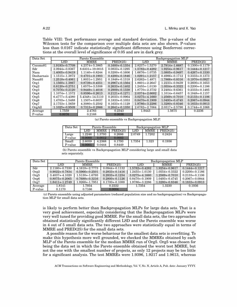
Firstly, let’s analyse the test performance average considering all data sets. TableVIII shows the average test performance and standard deviation for the Pareto en-semble and the Backpropagation MLP. The cells in light grey represent better averages(not necessarily statistically different). The table also shows the overall average andp-value of the Wilcoxon test used for the statistical comparison of all runs over mul-tiple data sets. P-values less than 0.0167 (shown in dark grey) indicate statisticallysignificant difference using Bonferroni corrections considering the three performancemeasures at the overall level of significance of 0.05. As we can see, the two approachesare statistically the same considering the overall MMRE, but different when consider-ing LSD and PRED(25). In the latter case, the Pareto ensemble wins in 7 out of 13 datasets considering LSD and PRED(25), as shown by the light grey cells. This number ofwins is similar to the number of losses, so additional analysis is necessary to betterunderstand the Pareto ensemble’s behaviour and check if it can be improved, as shownin the next paragraphs.
Hence, secondly, if we take a closer look, we can see that Backpropagation MLPfrequently wins for the smallest data sets, whereas the Pareto ensemble tends behavebetter for the largest data sets. Considering LSD, the Pareto ensemble wins in 6 out of8 large data sets. Considering MMRE, it wins in 5 out of 8 large data sets. ConsideringPRED(25), it wins in 7 out of 8 large data sets. So, we performed additional statisticaltests to compare the behaviour of all the runs considering the data sets with less than35 projects (sdr, org2, org5, org6, org7) and with 60 or more projects (cocomo81, nasa93,nasa, desharnais, org1, org3, org4, orgAll) separately.
Table VIIIb shows the overall averages and p-values for these two groups of datasets. We can see that there is statistically significant difference considering all per-formance measures for the large data sets, including MMRE. That together with thefact that the Pareto ensemble wins in most cases for these data sets indicates that it
ACM Transactions on Software Engineering and Methodology, Vol. V, No. N, Article A, Pub. date: January YYYY.
A:22 L. Minku and X. Yao
Table VIII: Test performance average and standard deviation. The p-values of theWilcoxon tests for the comparison over multiple data sets are also shown. P-valuesless than 0.0167 indicate statistically significant difference using Bonferroni correc-tions at the overall level of significance of 0.05 and are in dark grey.
Data Set Pareto Ensemble Backpropagation MLPLSD MMRE PRED(25) LSD MMRE PRED(25)
Cocomo81 1.9193+-0.7709 4.2374+-5.3865 0.1600+-0.1354 2.8237+-1.5270 2.7914+-1.6687 0.1300+-0.1179Sdr 2.0944+-0.8367 8.6331+-19.0015 0.0833+-0.1295 1.5782+-0.4282 1.9254+-0.9617 0.1444+-0.1217Nasa 1.4005+-0.9419 1.1140+-0.8244 0.3200+-0.1606 1.6676+-1.0735 1.0805+-0.9497 0.4267+-0.1530Desharnais 1.1515+-1.3872 0.4701+-0.1903 0.4200+-0.1846 1.0291+-1.2157 0.4986+-0.1712 0.3333+-0.1373Nasa93 1.2518+-0.4061 1.8031+-1.2951 0.1848+-0.1318 2.6262+-1.4871 1.7866+-0.8316 0.1970+-0.0927Org1 1.1560+-1.3867 0.8739+-0.4551 0.2967+-0.1564 1.8601+-2.2647 1.2233+-0.9439 0.2600+-0.1653Org2 0.8120+-0.2751 1.6575+-3.5308 0.2633+-0.1402 1.2455+-1.0130 1.0554+-0.3322 0.2200+-0.1186Org3 0.7076+-0.2120 0.9449+-1.4016 0.2909+-0.1338 1.8770+-2.3732 3.2484+-9.6361 0.2333+-0.1485Org4 1.1074+-1.1572 0.8596+-0.2613 0.2121+-0.1271 2.0374+-2.6682 1.1014+-0.6457 0.1848+-0.1157Org5 6.4777+-5.4380 5.4348+-14.5110 0.2033+-0.0964 3.0275+-4.1660 1.2569+-0.7010 0.2133+-0.1106Org6 1.4703+-1.5488 1.1507+-0.6037 0.1833+-0.1053 0.8470+-0.1909 1.0493+-0.4745 0.2067+-0.0944Org7 2.1753+-1.5659 4.3080+-5.2502 0.1633+-0.1129 1.9786+-3.2286 1.3280+-0.8346 0.1833+-0.0913OrgAll 1.1025+-0.9509 0.7313+-0.2866 0.2641+-0.1350 2.6782+-2.7064 2.0317+-2.5790 0.1744+-0.1068Average 1.7559 2.4783 0.2343 1.9443 1.5675 0.2236P-value 0.0076 0.2168 0.0036
(a) Pareto ensemble vs Backpropagation MLP.
Data Set Pareto Ensemble Backpropagation MLPLSD MMRE PRED(25) LSD MMRE PRED(25)
Large 1.2246 1.3793 0.2686 2.0749 1.7202 0.2424P-value 0.0000 0.0012 0.0003Small 2.6059 4.2368 0.1793 1.7354 1.323 0.1936P-value 0.0001 0.0444 0.8449
(b) Pareto ensemble vs Backpropagation MLP considering large and small datasets separately.
Data Set Pareto Ensemble Backpropagation MLPLSD MMRE PRED(25) LSD MMRE PRED(25)
Sdr 2.1160+-0.7330 4.1618+-2.7773 0.0944+-0.1132 1.5782+-0.4282 1.9254+-0.9617 0.1444+-0.1217Org2 0.9022+-0.7834 0.5966+-0.2501 0.2833+-0.1416 1.2455+-1.0130 1.0554+-0.3322 0.2200+-0.1186Org5 3.4037+-4.1020 1.5130+-1.6793 0.2833+-0.1234 3.0275+-4.1660 1.2569+-0.7010 0.2133+-0.1106Org6 0.8075+-0.2065 0.7688+-0.3216 0.2800+-0.1126 0.8470+-0.1909 1.0493+-0.4745 0.2067+-0.0944Org7 1.8411+-1.2749 1.9268+-1.7951 0.1700+-0.1088 1.9786+-3.2286 1.3280+-0.8346 0.1833+-0.0913Average 1.8141 1.7934 0.2222 1.7354 1.3230 0.1936P-value 0.1170 0.7166 0.0004
(c) Pareto ensemble using adjusted parameters (reduced population size and no backpropagation) vs Backpropaga-tion MLP for small data sets.
is likely to perform better than Backpropagation MLPs for large data sets. That is avery good achievement, especially considering that the Backpropagation MLPs werevery well tuned for providing good MMRE. For the small data sets, the two approachesobtained statistically significantly different LSD and the Pareto ensemble was worsein 4 out of 5 small data sets. The two approaches were statistically equal in terms ofMMRE and PRED(25) for the small data sets.
A possible reason for the worse behaviour for the smallest data sets is overfitting. Tomake this hypothesis more well grounded, we checked the MMREs obtained by eachMLP of the Pareto ensemble for the median MMRE run of Org5. Org5 was chosen forbeing the data set in which the Pareto ensemble obtained the worst test MMRE, butnot the one with the smallest number of projects, as only 12 projects may be too littlefor a significant analysis. The test MMREs were 1.9396, 1.9217 and 1.9613, whereas
ACM Transactions on Software Engineering and Methodology, Vol. V, No. N, Article A, Pub. date: January YYYY.

Software Effort Estimation as a Multi-objective Learning Problem A:23
the corresponding train MMREs were 0.0998, 0.0976 and 0.1017, respectively. We cansee that the test MMREs were drastically larger than the train MMREs. On the otherhand, the three runs on and around the median test MMRE for the BackpropagationMLPs obtained 1.0403, 1.0433 and 1.1599 test MMRE, whereas the train MMREswere 0.3183, 1.0857 and 0.1176. So, the train MMREs were higher (worse) for theBackpropagation MLPs than for the best fit Pareto MLPs. That indicates that theMOEA may indeed be overfitting when the data sets are too small. Besides the fact thatlearning is inherently hard due to the small number of training examples, a possiblecause for that is the parameters choice, as the parameters were not so well tuned forthe MOEA.
So, thirdly, additional MOEA runs were performed in such a way to use the essenceof the early stopping strategy to avoid overfitting [Finnoff et al. 1993]. This was done byreducing the population size from 100 to 30 and the number of epochs for the offspringBackpropagation from 5 to zero (no Backpropagation). The results are shown in tableVIIIc. As we can see, the Pareto ensemble obtained similar LSD and MMRE to Back-propagation MLPs. PRED(25) was statistically significantly different and the Paretoensemble won in 3 out of 5 data sets. The improvement in the overall average was ofabout 0.79 for LSD, 2.44 for MMRE and 0.04 for PRED(25). The test MMREs for themedian MMRE run of the Pareto ensemble for Org5 were 0.8649, 0.8528 and 1.4543,whereas the corresponding train MMREs were 0.3311, 0.3116 and 0.5427. These trainMMREs are closer to the corresponding test MMREs than when using the previousparameters configuration, indicating less overfitting.
Lastly, in order to check the performance of the Pareto ensemble for outlier projects,we have also tested it using test sets composed only of the outliers identified in sec-tion 6. The MMRE and PRED(25) obtained for the outlier sets were compared to theoriginal test sets’. It is not possible to compare LSD because the number of outliersis too small and LSD’s equation is divided by the number of projects minus one. So,even if the error obtained for the outlier sets is potentially smaller, the small numberof examples increases LSD.
The results show that PRED(25) was always worse for the outlier sets than for theoriginal test sets. That means that these outliers are projects to which the Paretoensemble has difficulties in predicting within 25% of the actual effort. However, theMMRE is actually better for 3 out of 9 data sets that involve outliers. So, in about athird of the cases, the outliers are not projects to which the Pareto ensemble obtainsthe worst performances. For the other cases, the MMRE was usually less than 0.27higher.
The analysis performed in this section shows that the use of MOEA for consideringseveral performance measures at the same time is successful in generating SEE en-sembles. The Pareto ensemble manages to obtain similar or better performance thanBackpropagation MLP across data sets in terms of all the measures used as objec-tives by the MOEA. So, it is worth considering the creation of SEE models as a multi-objective problem and the Pareto ensemble can be used when none of the performancemeasures is to be emphasized over the others.
9. EMPHASIZING PARTICULAR PERFORMANCE MEASURES
This section concentrates on answering RQ3. As shown in section 8, MOEA can be usedto automatically generate an ensemble that provides an ideal trade-off among differ-ent measures, so that the software manager does not need to decide on a particularsolution or performance measure. The main objective of the comparison presented inthe present section is to analyse whether we can further increase the test performancefor each measure separately if we wish to emphasize this particular measure. Thissection provides a better understanding of the solutions that can be produced by the
ACM Transactions on Software Engineering and Methodology, Vol. V, No. N, Article A, Pub. date: January YYYY.
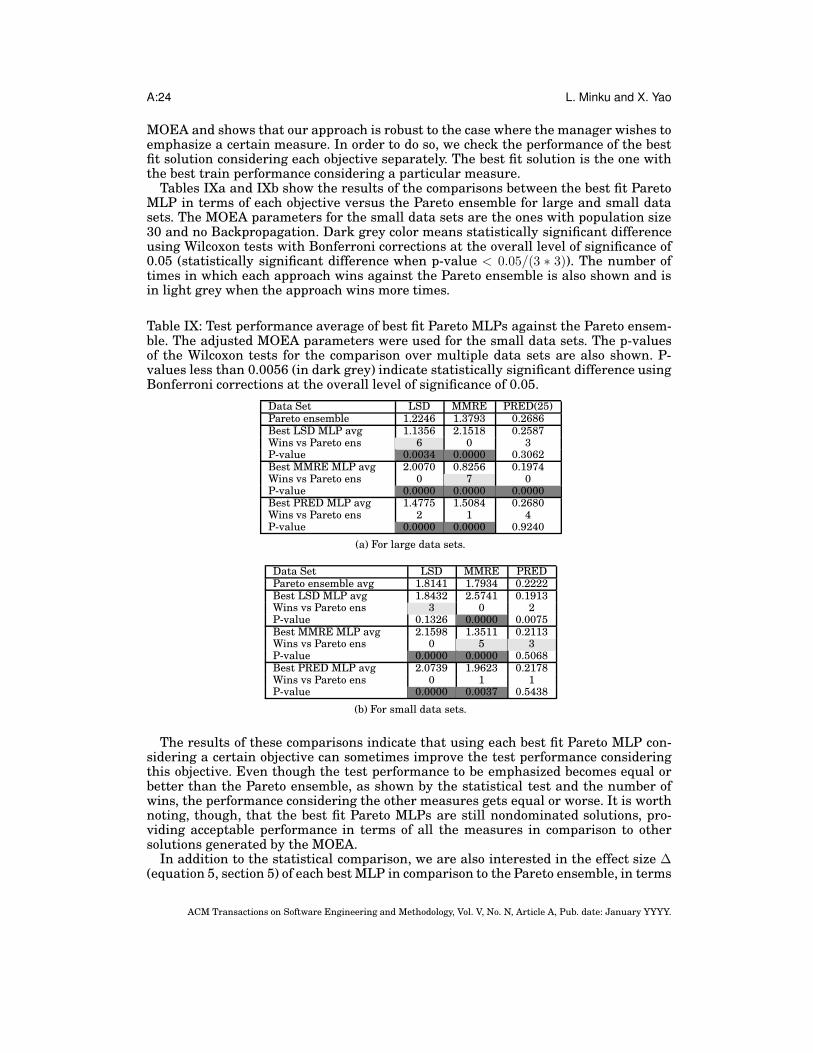
A:24 L. Minku and X. Yao
MOEA and shows that our approach is robust to the case where the manager wishes toemphasize a certain measure. In order to do so, we check the performance of the bestfit solution considering each objective separately. The best fit solution is the one withthe best train performance considering a particular measure.
Tables IXa and IXb show the results of the comparisons between the best fit ParetoMLP in terms of each objective versus the Pareto ensemble for large and small datasets. The MOEA parameters for the small data sets are the ones with population size30 and no Backpropagation. Dark grey color means statistically significant differenceusing Wilcoxon tests with Bonferroni corrections at the overall level of significance of0.05 (statistically significant difference when p-value < 0.05/(3 ∗ 3)). The number oftimes in which each approach wins against the Pareto ensemble is also shown and isin light grey when the approach wins more times.
Table IX: Test performance average of best fit Pareto MLPs against the Pareto ensem-ble. The adjusted MOEA parameters were used for the small data sets. The p-valuesof the Wilcoxon tests for the comparison over multiple data sets are also shown. P-values less than 0.0056 (in dark grey) indicate statistically significant difference usingBonferroni corrections at the overall level of significance of 0.05.
Data Set LSD MMRE PRED(25)Pareto ensemble 1.2246 1.3793 0.2686Best LSD MLP avg 1.1356 2.1518 0.2587Wins vs Pareto ens 6 0 3P-value 0.0034 0.0000 0.3062Best MMRE MLP avg 2.0070 0.8256 0.1974Wins vs Pareto ens 0 7 0P-value 0.0000 0.0000 0.0000Best PRED MLP avg 1.4775 1.5084 0.2680Wins vs Pareto ens 2 1 4P-value 0.0000 0.0000 0.9240
(a) For large data sets.
Data Set LSD MMRE PREDPareto ensemble avg 1.8141 1.7934 0.2222Best LSD MLP avg 1.8432 2.5741 0.1913Wins vs Pareto ens 3 0 2P-value 0.1326 0.0000 0.0075Best MMRE MLP avg 2.1598 1.3511 0.2113Wins vs Pareto ens 0 5 3P-value 0.0000 0.0000 0.5068Best PRED MLP avg 2.0739 1.9623 0.2178Wins vs Pareto ens 0 1 1P-value 0.0000 0.0037 0.5438
(b) For small data sets.
The results of these comparisons indicate that using each best fit Pareto MLP con-sidering a certain objective can sometimes improve the test performance consideringthis objective. Even though the test performance to be emphasized becomes equal orbetter than the Pareto ensemble, as shown by the statistical test and the number ofwins, the performance considering the other measures gets equal or worse. It is worthnoting, though, that the best fit Pareto MLPs are still nondominated solutions, pro-viding acceptable performance in terms of all the measures in comparison to othersolutions generated by the MOEA.
In addition to the statistical comparison, we are also interested in the effect size ∆(equation 5, section 5) of each best MLP in comparison to the Pareto ensemble, in terms
ACM Transactions on Software Engineering and Methodology, Vol. V, No. N, Article A, Pub. date: January YYYY.

Software Effort Estimation as a Multi-objective Learning Problem A:25
of the performance measure for which the MLP performs best. Table X presents theminimum, maximum, average and standard deviation of the effect size ∆, as well asthe number of data sets for which the effect size was small, medium or large. Eventhough using each best MLP separately can provide some improvement in perfor-mance, the improvements are usually small. Nevertheless, as it would be very easyto configure an approach to use the best MLPs instead of the Pareto ensemble, onemay wish to use the best MLPs to emphasize a certain performance measure evenconsidering that the improvement in performance is small.
Table X: Effect size for each best MLP against the Pareto ensemble, in terms of theperformance measure for which the MLP performs best.
Min ∆ Max ∆ Avg. ∆ Std. ∆ # Small # Medium # Large # Medium+LargeBest LSD MLP 0.0257 0.3221 0.1395 0.0993 8 0 0 0Best MMRE MLP 0.0046 0.7983 0.3462 0.3035 4 3 1 4Best PRED MLP 0.0542 0.2953 0.1699 0.0987 8 0 0 0
(a) Large data sets
Min ∆ Max ∆ Avg. ∆ Std. ∆ # Small # Medium # Large # Medium+LargeBest LSD MLP 0.0294 0.4468 0.2009 0.1687 4 1 0 1Best MMRE MLP 0.0567 0.5913 0.2665 0.2080 4 1 0 1Best PRED MLP 0.0235 0.9502 0.4050 0.3977 2 1 2 3
(b) Small data sets
10. FURTHER ANALYSIS OF THE MODEL CHOICE
The main objective of the comparison presented in this section is to analyse whetherour approach still has room for improvement in terms of model choice. If so, as futurework, other methods for choosing models for the Pareto ensemble should be investi-gated with the aim of improving this approach further. In order to make this analysis,we used the best Pareto MLPs according to each test performance. These MLPs rep-resent the best possible choice of solutions generated by the MOEA considering eachobjective separately. A Pareto ensemble composed of these MLPs was also formed. Ta-bles XIa and XIb show the results of the comparisons. Again, the parameters usedby the MOEA for the small data sets here are the ones with population size 30 andno Backpropagation. Wilcoxon tests with Bonferroni corrections at the overall signifi-cance level of 0.05 (statistically significant difference when p-value < 0.05/(3 ∗ 4)) wereused to aid the comparison.
We can see that there are test performance improvements in almost all cases, bothwhen using the best Pareto MLPs by themselves and when combining them into aPareto ensemble. In particular, for most results with statistically significant differencein the average LSD, MMRE or PRED(25), the best test performance approach winsmore times than the Backpropagation MLPs. This analysis shows that, even thoughour approach can significantly reduce overfitting by reducing the population size andeliminating offspring Backpropagation for smaller data sets, simply choosing the bestfit Pareto MLPs according to the train performance still does not necessarily lead to thebest achievable performance. As future work, other strategies to chose models amongthe Pareto solutions should be investigated to improve the performance even further.
11. COMPARISON AGAINST OTHER TYPES OF MODELS
The main objectives of RQ2 and RQ3 were to show that MOEAs can be used to evolvemodels considering different performance measures at the same time, being able to
ACM Transactions on Software Engineering and Methodology, Vol. V, No. N, Article A, Pub. date: January YYYY.

A:26 L. Minku and X. Yao
Table XI: Test performance average of best test performing Pareto MLPs against Back-propagation MLP. The adjusted MOEA parameters were used for the small data sets.The p-values of the Wilcoxon tests for the comparison over multiple data sets are alsoshown. P-values less than 0.0042 (in dark grey) indicate statistically significant differ-ence using Bonferroni corrections at the overall level of significance of 0.05.
Data Set LSD MMRE PRED(25)Backprop MLP 2.0749 1.7202 0.2424MLP Best LSD 0.8651 1.363 0.2994Wins vs Backprop MLP 8 6 7P-value 0.0000 0.0004 0.0000MLP Best MMRE 1.4759 0.6423 0.31Wins vs Backprop MLP 7 8 7P-value 0.0031 0.0000 0.0000MLP Best PRED 1.241 1.0735 0.437Wins vs Backprop MLP 8 6 8P-value 0.0000 0.0000 0.0000Pareto ensemble 0.9951 0.9649 0.3272Wins vs Backprop MLP 7 5 6P-value 0.0000 0.0000 0.0000
(a) For large data sets.
Data Set LSD MMRE PRED(25)Backprop MLP 1.7354 1.323 0.1936MLP Best LSD 1.3761 1.4272 0.2267Wins vs Backprop MLP 5 2 4P-value 0.0001 0.0812 0.0001MLP Best MMRE 1.8198 1.0558 0.2496Wins vs Backprop MLP 1 4 4P-value 0.3141 0.0000 0.0000MLP Best PRED 1.785 1.4286 0.3489Wins vs Backprop MLP 2 2 5P-value 0.5729 0.0043 0.0000Pareto ensemble 1.5671 1.2636 0.2482Wins vs Backprop MLP 3 2 3P-value 0.1653 0.0011 0.0000
(b) For small data sets.
produce solutions that achieve good results in comparison to a traditional algorithmthat does not use several different measures explicitly to generate the same type ofmodels, besides being flexible to allow emphasizing different performance measures.The analyses explained in sections 8 and 9 answer RQ2 and RQ3. Nevertheless, eventhough it is not the key point of this paper, it is still interesting to know how wellMOEAs to evolve MLPs behave in comparison to other types of model. Differentlyfrom the previous analysis, such a comparison mixes the evaluation of the MOEA tothe evaluation of the underlying model being evolved (MLP).
In this section, we present a comparison of the Pareto ensemble to several differenttypes of model besides MLPs: RBFs, RTs, EBA with log transformed data, Baggingwith MLPs, Bagging with RBFs, Bagging with RTs, Random with MLPs and NCLwith MLPs, as explained in section 5. For this comparison, the parameters used by theMOEA on the small data sets were adjusted to population size of 30 and no offspringBackpropagation. The performance measures used to evaluate the models are LSD,MMRE, PRED(25), MdMRE, MAE and MdAE.
The first step of our analysis consists in performing Friedman tests [Demsar 2006]for the statistical comparison of multiple models over multiple data sets for each per-formance measure. The null hypothesis is that all the models perform similarly ac-
ACM Transactions on Software Engineering and Methodology, Vol. V, No. N, Article A, Pub. date: January YYYY.
Software Effort Estimation as a Multi-objective Learning Problem A:27
cording to the measure considered. The tests rejected the null hypothesis for the sixperformance measures with Holm-Bonferroni corrections at the overall level of sig-nificance of 0.05. The Friedman tests also provide rankings of the approaches acrossdata sets, which show that Pareto ensemble, bagging +MLPs, log + EBA and RTs havethe top half average ranks considering all measures but LSD. Models based on MLPs,including the Pareto ensemble, tend to be lower ranked considering LSD. A closer anal-ysis of the MLPs revealed that they can sometimes make negative estimations, whichhave a strong impact on LSD. RTs, on the other hand, can never give negative estima-tions or estimations close to zero when the training data does not contain such effortvalues. So, learners based on RTs obtained in general better LSD. Bagging + RTs isthe highest ranked approach in terms of both LSD and MAE.
It is important to note that MOEAs could also be used to evolve other types of struc-ture than MLPs. However, the key point of this paper is the investigation of the multi-objective formulation of the problem of creating SEE models and obtaining a betterunderstanding of the performance measures. The use MOEA to evolve other types ofmodel such as RTs, which could improve LSD, is proposed as future work.
It is also interesting to verify the standard deviation of the Friedman ranking acrossdifferent performance measures. The Pareto ensemble and log + EBA presented themedian standard deviation, meaning that their average ranking across data sets doesnot vary too much when considering different performance measures, even though theyare not the approaches that vary the least. Bagging + MLPs presented the lowest andbagging + RTs presented the highest standard deviation.
Nevertheless, simply looking at the ranking provided by the Friedman test is notvery descriptive for SEE, as the models tend to behave very differently depending onthe data set. Ideally, we would like to use the approach that is most suitable for thedataset in hands. So, as the second step of our analysis, we determine what approachesare ranked first according to the test performance on each data set separately. Thisis particularly interesting because it allows us to identify on what type of data setsa certain approach behaves better. Table XIIa shows the approaches ranked as firstconsidering each data set and performance measure. Table XIIb helps us to see thatthe Pareto ensemble appears more often as the first than the other approaches in termsof all measures but LSD. Table XIIc shows that the Pareto ensemble is never rankedlast more than twice considering all 13 data sets and it is only ranked worse twicein terms of MMRE. For the reason explained in the previous paragraphs, approachesbased on MLPs are rarely ranked first in terms of LSD, whereas bagging + RTs andRTs are the approaches that appear most often as first in terms of this measure.
Table XIIa also reveals that the Pareto ensemble was first more often for the ISBSGdata sets than for the PROMISE data sets. ISBSG data sets are considered as veryheterogeneous. So, MOEAs might be particularly useful for more heterogeneous data.A possible reason for that is that the Pareto ensemble uses a global optimisation algo-rithm, which is usually better at identifying the most promising regions of the searchspace than local algorithms such as Backpropagation. More heterogeneous data setsmay present search surfaces with several peaks, more difficult to tackle by local searchalgorithms.
As a third step of our analysis, the absolute value of the effect size ∆ (equation 5,section 5) using MAE as the performance measure were calculated (table XIII). Wereport ∆ based on MAE because this performance measure is symmetric/unbiased. Aswe can see, many of the effect sizes are medium or large. So, the choice of a certainapproach instead of the Pareto ensemble can have a big impact on the performance ofthe SEEs.
Finally, it is also worth noting that, in terms of computational time, some approachessuch as log + EBA are faster than the MOEA. However, we do not consider the differ-
ACM Transactions on Software Engineering and Methodology, Vol. V, No. N, Article A, Pub. date: January YYYY.

A:28 L. Minku and X. Yao
Table XII: Approaches ranked as first.
Approach LSD MMRE PRED(25) MdMRE MAE MdAECocomo81 RT Bag+MLP Bag+MLP Bag+ MLP Bag + MLP Bag + MLPSdr RT RT Bag+RT RT RT RBFNasa Bag+RT RT Bag+MLP Bag + MLP Bag +RT Bag + RTDesharnais Bag+RT Bag+MLP Pareto Ens Pareto Ens Pareto Ens Pareto EnsNasa93 RT RT RT RT RT RTOrg1 Bag+RBF Pareto Ens Pareto Ens Pareto Ens Pareto Ens Pareto EnsOrg2 Bag+RT Pareto Ens Pareto Ens Pareto Ens Pareto Ens Pareto EnsOrg3 Pareto Ens Pareto Ens Log + EBA Log + EBA Log + EBA Log + EBAOrg4 Bag+RBF Pareto Ens RT RT Pareto Ens Pareto EnsOrg5 Bag+RT Log + EBA Bag+RBF Rand + MLP Bag + RT RTOrg6 Bag+RBF Pareto Ens Pareto Ens Pareto Ens Bag + RBF Pareto EnsOrg7 Bag+RT Log + EBA Log + EBA Log + EBA Bag + RBF Pareto EnsOrgAll RT Pareto Ens Pareto Ens Pareto Ens Pareto Ens Pareto Ens
(a) Approaches per data set.
Approach LSD MMRE PRED(25) MdMRE MAE MdAEPareto Ens 1 6 5 5 5 7RT 4 3 2 3 2 2Bag+RT 5 0 1 0 2 1Bag+MLP 0 2 2 2 1 1Log + EBA 0 2 2 2 1 1Bag+RBF 3 0 1 0 2 0Rand+MLP 0 0 0 1 0 0RBF 0 0 0 0 0 1Total 13 13 13 13 13 13
(b) Total number of times ranked as first per approach. Approaches never ranked as first are omitted.Values higher than 3 are highlighted in grey.
Approach LSD MMRE PRED(25) MdMRE MAE MdAEBag + MLP 0 0 0 0 1 0MLP 1 0 1 0 0 0RT 0 0 0 1 1 0Bag + RT 0 1 1 0 0 1Pareto Ens 1 2 0 1 1 1Rand + MLP 2 1 1 2 1 1Bag + RBF 0 3 3 2 0 2RBF 1 2 4 3 4 3NCL 8 4 3 4 5 5Total 13 13 13 13 13 13
(c) Total number of times ranked as last per approach. Approaches never ranked as last areomitted. Values higher than 3 are highlighted in grey.
Table XIII: Effect size for each approach against the Pareto ensemble.
Approach Min ∆ Max ∆ Avg. ∆ Std. ∆ # Small # Medium # Large # Medium+LargeBag+MLP 0.0296 0.9194 0.3775 0.2839494668 7 4 2 6Bag+RBF 0.0046 1.3072 0.5007 0.4233246489 6 3 4 7Bag+RT 0.0518 1.3383 0.4842 0.4195283097 7 3 3 6Log + EBA 0.0199 1.4054 0.5333 0.4839488764 7 2 4 6MLP 0.0202 1.5049 0.4155 0.4034613873 7 3 3 6NCL 0.0170 2.4236 0.7194 0.6534745379 5 3 5 8Rand 0.0720 1.5655 0.4615 0.4444167846 7 3 3 6RBF 0.0393 1.5730 0.6207 0.5299600056 6 2 5 7RT 0.0392 1.8151 0.5614 0.5203035024 4 6 3 9
ACM Transactions on Software Engineering and Methodology, Vol. V, No. N, Article A, Pub. date: January YYYY.
Software Effort Estimation as a Multi-objective Learning Problem A:29
ences as of practical significance, because our approach did not present high runningtime. The reasons for the low running time are (1) SEE data sets are usually small incomparison to other ML applications and (2) our results were obtained without run-ning the MOEA for too many generations. As an example, one run for the largest, thesecond largest and the third largest data sets, which use 20, 100 and 200 generations,respectively, takes less than 1 minute to finish.
In summary, this section shows that MOEA-evolved MLPs are able to achieve com-petitive results in comparison to other approaches in the literature. The Pareto en-semble usually obtained comparatively good results in terms of all measures but LSD.Whether this is acceptable is problem (project) dependent and also depends on themagnitude of loss in terms of LSD compared to the gain in other measures. Moreover,the Pareto ensemble seems to perform better for more heterogeneous data sets such asISBSG.
12. CONCLUSIONS
This paper proposes and demonstrates how to view the problem of creating SEE mod-els through a different perspective, by tackling it as a multi-objective problem that con-siders different performance measures explicitly and simultaneously. Using a MOEAto solve this problem allows us to better understand different performance measuresand to produce SEE models with good overall performance in comparison to a modelthat does not consider these measures explicitly.
As an answer to RQ1, we show that LSD and MMRE are performance measures withsomewhat opposite behaviour. Moreover, models with similar LSD/MMRE are likelyto present different PRED(25) and vice-versa. So, one may wish to choose a modelthat does not behave particularly bad for any intended performance measures. This isone of the motivations for our approach to use MOEAs, as MOEAs consider all theseperformance measures at the same time. This difference in behaviour also providesthe second motivation for our approach: it can produce diverse ensembles, which aremore likely to have increased performance.
The results above indicate that considering different performance measures explic-itly when creating a model may be used to produce good ensembles. As an answer toRQ2, we show that indeed a MOEA can be used to create models by explicitly consid-ering different performance measures at the same time. Pareto ensemble of MLPs pro-duced by a MOEA generally obtained similar or better performance than Backpropa-gation MLPs considering both LSD, MMRE and PRED(25). The average performanceswere generally better for the data sets with 60 or more projects.
As an answer to RQ3, we show that MOEAs are also flexible, allowing the softwaremanager to choose models that emphasize certain performance measures over the oth-ers, if s/he desires to do so. A MOEA can be used to produce and choose models thatemphasize a particular measure without completely ignoring the performance usingother measures, whereas the Pareto ensemble can be used as a good trade-off amongmeasures, if the software manager does not wish to emphasize any particular measure.
As shown in our comparison of the Pareto ensemble against Backpropagation MLPs,which produce the same type of model as the MOEA, the Pareto ensemble has shown tobe useful for both single and multi-company data sets. Our comparison against modelsof a different type than the base models evolved by the MOEA further shows thatMOEAs may be particularly useful for more heterogeneous data sets. They can maketypes of models that would usually not be ranked first in terms of performance becomeranked first through the Pareto ensemble.
Our proposed methodology still has room for improvements in terms of the choice ofmodels to compose the Pareto ensemble. The investigation of new strategies is left asfuture work, as well as the experimentation of our approach using different MOEAs
ACM Transactions on Software Engineering and Methodology, Vol. V, No. N, Article A, Pub. date: January YYYY.
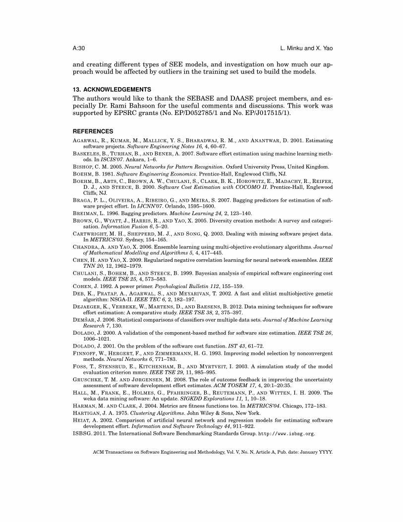
A:30 L. Minku and X. Yao
and creating different types of SEE models, and investigation on how much our ap-proach would be affected by outliers in the training set used to build the models.
13. ACKNOWLEDGEMENTS
The authors would like to thank the SEBASE and DAASE project members, and es-pecially Dr. Rami Bahsoon for the useful comments and discussions. This work wassupported by EPSRC grants (No. EP/D052785/1 and No. EP/J017515/1).
REFERENCES
AGARWAL, R., KUMAR, M., MALLICK, Y. S., BHARADWAJ, R. M., AND ANANTWAR, D. 2001. Estimatingsoftware projects. Software Engineering Notes 16, 4, 60–67.
BASKELES, B., TURHAN, B., AND BENER, A. 2007. Software effort estimation using machine learning meth-ods. In ISCIS’07. Ankara, 1–6.
BISHOP, C. M. 2005. Neural Networks for Pattern Recognition. Oxford University Press, United Kingdom.
BOEHM, B. 1981. Software Engineering Economics. Prentice-Hall, Englewood Cliffs, NJ.
BOEHM, B., ABTS, C., BROWN, A. W., CHULANI, S., CLARK, B. K., HOROWITZ, E., MADACHY, R., REIFER,D. J., AND STEECE, B. 2000. Software Cost Estimation with COCOMO II. Prentice-Hall, EnglewoodCliffs, NJ.
BRAGA, P. L., OLIVEIRA, A., RIBEIRO, G., AND MEIRA, S. 2007. Bagging predictors for estimation of soft-ware project effort. In IJCNN’07. Orlando, 1595–1600.
BREIMAN, L. 1996. Bagging predictors. Machine Learning 24, 2, 123–140.
BROWN, G., WYATT, J., HARRIS, R., AND YAO, X. 2005. Diversity creation methods: A survey and categori-sation. Information Fusion 6, 5–20.
CARTWRIGHT, M. H., SHEPPERD, M. J., AND SONG, Q. 2003. Dealing with missing software project data.In METRICS’03. Sydney, 154–165.
CHANDRA, A. AND YAO, X. 2006. Ensemble learning using multi-objective evolutionary algorithms. Journalof Mathematical Modelling and Algorithms 5, 4, 417–445.
CHEN, H. AND YAO, X. 2009. Regularized negative correlation learning for neural network ensembles. IEEETNN 20, 12, 1962–1979.
CHULANI, S., BOHEM, B., AND STEECE, B. 1999. Bayesian analysis of empirical software engineering costmodels. IEEE TSE 25, 4, 573–583.
COHEN, J. 1992. A power primer. Psychological Bulletin 112, 155–159.
DEB, K., PRATAP, A., AGARWAL, S., AND MEYARIVAN, T. 2002. A fast and elitist multiobjective geneticalgorithm: NSGA-II. IEEE TEC 6, 2, 182–197.
DEJAEGER, K., VERBEKE, W., MARTENS, D., AND BAESENS, B. 2012. Data mining techniques for softwareeffort estimation: A comparative study. IEEE TSE 38, 2, 375–397.
DEMSAR, J. 2006. Statistical comparisons of classifiers over multiple data sets. Journal of Machine LearningResearch 7, 130.
DOLADO, J. 2000. A validation of the component-based method for software size estimation. IEEE TSE 26,1006–1021.
DOLADO, J. 2001. On the problem of the software cost function. IST 43, 61–72.
FINNOFF, W., HERGERT, F., AND ZIMMERMANN, H. G. 1993. Improving model selection by nonconvergentmethods. Neural Networks 6, 771–783.
FOSS, T., STENSRUD, E., KITCHENHAM, B., AND MYRTVEIT, I. 2003. A simulation study of the modelevaluation criterion mmre. IEEE TSE 29, 11, 985–995.
GRUSCHKE, T. M. AND JØRGENSEN, M. 2008. The role of outcome feedback in improving the uncertaintyassessment of software development effort estimates. ACM TOSEM 17, 4, 20:1–20:35.
HALL, M., FRANK, E., HOLMES, G., PFAHRINGER, B., REUTEMANN, P., AND WITTEN, I. H. 2009. Theweka data mining software: An update. SIGKDD Explorations 11, 1, 10–18.
HARMAN, M. AND CLARK, J. 2004. Metrics are fitness functions too. In METRICS’04. Chicago, 172–183.
HARTIGAN, J. A. 1975. Clustering Algorithms. John Wiley & Sons, New York.
HEIAT, A. 2002. Comparison of artificial neural network and regression models for estimating softwaredevelopment effort. Information and Software Technology 44, 911–922.
ISBSG. 2011. The International Software Benchmarking Standards Group. http://www.isbsg.org.
ACM Transactions on Software Engineering and Methodology, Vol. V, No. N, Article A, Pub. date: January YYYY.

Software Effort Estimation as a Multi-objective Learning Problem A:31
JORGENSEN, M. AND SHEPPERD, M. 2007. A systematic review of software development cost estimationstudies. IEEE TSE 33, 1, 33–53.
JRGENSEN, M. AND GRIMSTAD, S. 2011. The impact of irrelevant and misleading information on softwaredevelopment effort estimates: A randomized controlled field experiment. IEEE TSE 37, 5, 695–707.
KHARE, V., YAO, X., AND DEB, K. 2003. Performance scaling of multi-objective evolutionary algorithms.In 2nd International Conference on Evolutionary Multi-Criterion Optimization (EMO’03), Lecture Notesin Computer Science, C. M. Fonseca, P. J. Fleming, E. Zitzler, K. Deb, and L. Thiele, Eds. Vol. 2632.Springer-Verlag, 376–390.
KOCAGUNELI, E., BENER, A., AND KULTUR, Y. 2009. Combining multiple learners induced on multipledatasets for software effort prediction. In ISSRE’07. Mysuru, India, 6p.
KOCAGUNELI, E., MENZIES, T., AND KEUNG, J. 2011. On the value of ensemble effort estimation. IEEETSE (inpress), 14p.
KULTUR, Y., TURHAN, B., AND BENER, A. 2009. Ensemble of neural networks with associative memory(ENNA) for estimating software development costs. Knowledge-Based Systems 22, 395–402.
L. I, . K. AND WHITAKER, C. J. 2003. Measures of diversity in classifier ensembles and their relationshipwith the ensemble accuracy. Machine Learning 51, 181–207.
LEGG, S., HUTTER, M., AND KUMAR, A. 2004. Tournament versus fitness uniform selection. In Proceedingsof the Congress of Evolutionary Computation (CEC). 2144–2151.
LIU, Y. AND YAO, X. 1999a. Ensemble learning via negative correlation. Neural Networks 12, 1399–1404.
LIU, Y. AND YAO, X. 1999b. Simultaneous training of negatively correlated neural networks in an ensemble.IEEE TSMC - Part B: Cybernetics 29, 6, 716–725.
LUKASIEWYCZ, M., GLA, M., REIMANN, F., AND HELWIG, S. 2011. Opt4j: The meta-heuristic optimisationframework for java. http://opt4j.sourceforge.net.
MENZIES, T., CHEN, Z., HIHN, J., AND LUM, K. 2006. Selecting best practices for effort estimation. IEEETSE 32, 11, 883–895.
MENZIES, T. AND SHEPPERD, M. 2012. Special issue on repeatable results in software engineering predic-tion. ESE 17, 17:1–17.
MILLER, B. L. AND GOLDBERG, D. E. 1995. Genetic algorithms, tournament selection, and the effects ofnoise. Complex Systems 9, 3, 193–212.
MINKU, L. L. May 2011. Machine learning for software effort estimation. The 13th CREST Open WorkshopFuture Internet Testing (FITTEST) & Search Based Software Engineering (SBSE), http://crest.cs.ucl.ac.uk/cow/13/slides/presentation_leandro.pdf, http://crest.cs.ucl.ac.uk/cow/13/videos/M2U00270Minku.mp4.
MINKU, L. L. AND YAO, X. 2011. A principled evaluation of ensembles of learning machines for softwareeffort estimation. In PROMISE’11. Banff, Canada, 10p.
MINKU, L. L. AND YAO, X. 2012. Ensembles and locality: Insight on improving software effort estimation.Submitted to IST, 38p.
MOHAGHEGHI, P., ANDA, B., AND CONRADI, R. 2005. Effort estimation of use cases for incremental large-scale software development. In ICSE. St. Louis, Missouri, 303–311.
MONTGOMERY, D. C. 2004. Design and Analysis of Experiments 6th Ed. John Wiley and Sons, Great Britain.
PRADITWONG, K., HARMAN, M., AND YAO, X. 2011. Software module clustering as a multi-objective searchproblem. IEEE Transactions on Software Engineering 37, 2, 264–282.
PRADITWONG, K. AND YAO, X. 2006. A new multi-objective evolutionary optimisation algorithm: the two-archive algorithm. In International Conference on Computational Intelligence and Security (CIS’2006).Vol. 1. Guangzhou, China, 286–291.
ROSENTHAL, R. 1994. The Handbook of Research Synthesis. Vol. 236. Sage, New York.
SEO, Y.-S., YOON, K.-A., AND BAE, D.-H. 2008. An empirical analysis of software effort estimation withoutlier elimination. In PROMISE. Leipzig, 25–32.
SHAN, Y., MCKAY, R. J., LOKAN, C. J., AND ESSAM, D. L. 2002. Software project effort estimation usinggenetic programming. In ICCCAS & WESINO EXPO. Vol. 2. Chengdu Sichuan, China, 1108–1112.
SHEPPERD, M. AND SCHOFIELD, C. 1997. Estimating software project effort using analogies. IEEETSE 23, 12, 736–743.
SHIRABAD, J. S. AND MENZIES, T. 2005. The PROMISE Repository of Software EngineeringDatabases. School of Information Technology and Engineering, University of Ottawa, Canada,http://promise.site.uottawa.ca/SERepository.
SRINIVAS, N. AND DEB, K. 1994. Multiobjective optimization using nondominated sorting in genetic algo-rithms. Evolutionary Computation 2, 221–248.
ACM Transactions on Software Engineering and Methodology, Vol. V, No. N, Article A, Pub. date: January YYYY.

A:32 L. Minku and X. Yao
SRIVASAN, K. AND FISHER, D. 1995. Machine learning approaches to estimating software developmenteffort. IEEE TSE 21, 2, 126–137.
TAN, H. B. K., ZHAO, Y., AND ZHANG, H. 2006. Estimating LOC for information systems from their con-ceptual data models. In ICSE. Shanghai, 321–330.
TAN, H. B. K., ZHAO, Y., AND ZHANG, H. 2009. Conceptual data model-based software size estimation forinformation systems. ACM TOSEM 19, 2, 4:1–4:37.
TRONTO, I. F. B., SILVA, J. D. S., AND SANT’ANNA, N. 2007. Comparison of artificial neural network andregression models in software effort estimation. In IJCNN’07. Orlando, 771–776.
WANG, Z., TANG, K., AND YAO, X. 2010. Multi-objective approaches to optimal testing resource allocationin modular software systems. IEEE TR 59, 3, 563–575.
WITTIG, G. E. AND FINNIE, G. R. 1994. Using artificial neural networks and function points to estimate4GL software development effort. Australian J. Information Systems 1, 2, 87–94.
WITTIG, G. E. AND FINNIE, G. R. 1997. Estimating software development effort with connectionist models.Information and Software Technology 39, 469–476.
ZHAO, Y. AND ZHANG, Y. 2008. Comparison of decision tree methods for finding active objects. Advances inSpace Research 41, 1955–1959.
ZITZLER, E., LAUMANNS, M., AND THIELE, L. 2002. SPEA2: Improving the strength pareto evolutionaryalgorithm. Evolutionary Methods for Design, Optimization and Control with Applications to IndustrialProblems (EUROGEN’2002), 95100.
ACM Transactions on Software Engineering and Methodology, Vol. V, No. N, Article A, Pub. date: January YYYY.
Related Documents