Stevens Institute of Technology School of Business Business Intelligence & Analytics Program A Snapshot of Data Science Student Poster Presentations Corporate Networking Event – November 27, 2018

Welcome message from author
This document is posted to help you gain knowledge. Please leave a comment to let me know what you think about it! Share it to your friends and learn new things together.
Transcript

Stevens Institute of TechnologySchool of Business
Business Intelligence & Analytics Program
A Snapshot of Data Science Student Poster Presentations
Corporate Networking Event – November 27, 2018
No. Title Student Authors
1* The Business Intelligence & Analytics Program BI&A Faculty, Weiyi Chen, Shiyue Ren
2 HSFL: Technology to Support Teaching & Research HSFL Faculty
3 Integrated Marketing Plan: Pennsylvania Market LLC Shuting Zhang
4* UBS WM Branch Prediction Shuting Zhang, Harsh Kava
5Employee Branding Research Glassdoor.com Company reviews analysis Shuting Zhang, Siyan Zhang
6 Analysis of Olympic athletes' data in 120 years history Yanzhao Liang, Yingjian Song, Hao Xu, Zhihao Yang
7 Predicting the outcome of a shot Haitao Liu, Yang Liu, Jiawei Xue
8*Predicted churn rate reduction for Telephone Services using Marketing Analytics
Jiawei Xue, Sucharitha Batchu, Suguna Bontha, Suprajah Suresh, Yang Liu
9Budget allocation optimization for natural disaster preparation Haohan Hu, Jiahao Shi, Lianhong Deng, Nifan Yuan
10Revenue and Cost Optimization for a Clothing Supply Chain Liran Zhang, Mingxin Zheng, Weifeng Li, Zeyu Shao
11Trip Master: A configuration tool for designing travel experience in New York
Shunyu Zheng, Sisi Xiong, Xinghong Liu, Yang Wu, Yiyi Liang
12 Predicting Airbnb Prices in Washington D.C.
Ankur Morbale, Matthew Rudolph, Kyle Eifler, Victoria Piskarev, Arthur Krivoruk, Gaurav Venkataraman, Sarvesh Gohil
13 Function Approximation Using Evolutionary Polynomials Aleksandr Grin
14Correlating Long-Term Innovation with Success in Career Progression Adam Coscia
15 Car Sales Analysis Lulu Zhu, Xin Chen, Yifeng Liu, Yuyi Yan
16 NBA Data Visualization Analysis Xin Chen, Xiaohao Su, Xiang Yang
17 Hot Wheels Analysis at NYC Yellow Taxi Abhitej Kodali, Nikhil Lohiya
18 Customer Revenue Prediction for Google Store Products Abhitej Kodali, Nikhil Lohiya
19Clustering Large Cap Stocks During Different Phases of the Economic Cycle Nikhil Lohiya, Raj Mehta
20* FIN-FINICKY : Financial Analyst’s Toolkit Nikhil Lohiya
21 Group Emailing using Robotic Process Automation Pallavi Naidu, Abhitej Kodali
22Cognitive Application to Determine Adverse Side Effects of Vaccines Pallavi Naidu, Kathy Chowaniec, Krishanu Agrawal
23Predict Potential Customers by Analyzing Bank’s Telemarketing Data Shreyas Menon, Pallavi Naidu
INDEX TO POSTERS
* Indicates the poster was accompanied by a live demo
24Quora - Answer Recommendation Using Deep Learning Models Tsen-Hung Wu, Cheng Yu, Shreyas Menon
25Lending Club – How to Forecast the Loan Status of Loan Applications. Tsen-Hung Wu, Shreyas Menon
26 Visualization of Chicago Crime Zihan Chen, Xuanyan Li
27 Predictive Model for House Pricing Zihan Chen, Xuanyan Li
28 DOE for Amazon Recommendation Email Siyan Zhang, Biyan Xie, Xuanyan Li
29 Predicting trends in bike sharing program Zixuan Wang, Shuqiong Chen, Kevin Walsh
30 NBA player management OptimizationJingchen Lan, Shan Jiang, Shuqiong Chen, Zixuan Wang
31 Improvement of medical wire manufacturing Zixuan Wang, Jingchen Lan
32 Identify the safety level of precincts in New York City Tianyu Liu, Chen Liao, Yu Hong, Xiangxiang He
33* Credit Analysis: Loan Default Prediction Jimit Sanghvi, Ho Ben Wesley Cheung, XinhangWang
34 Better Photography using Design of ExperimentsKumar Bipulesh, Ping-Lun Yeh, Sibo Xu, Sanjay Kumar Pattanayak
35 Driver Safety using CNN & Transfer Learning Kumar Bipulesh
36 Machine Learning to Predict US GC Sanjay Pattanayak, Smriti Vimal
37*UBS Pitch 2018 1st Prize Winners Machine Learning & Automation
Monica Vijaywargi, Poojan Gajera, Rohan Gala, Sanjay Pattanayak, Xunyan Li
38 Classifying Restaurant Rating Xiaojun zhu, Jhao-Han Chen, Haiping Sun
39Consumer Analytics for Restaurant Preferences using Yelp User Reviews Xiaojun Zhu, Haodong Zhao, Yuhan Su
40 Portfolio Optimization using PythonJhao-Han Chen, Jiamei Wang, Liang An, Ming Wei, Xuanzhu Luo
41* Radiology Assistant Amit Kumar, Jayesh Mehta, Yash Wanve
42Predicting Change in Bitcoin Prices Using Public Sentiment of the Cryptocurrency on Twitter
Thomas Treshock, Michael Ficke, Robert Frusina
43Surface-Enhancement Raman Scattering of Urine for Risk Assessment of Prostate Cancer Yiwei Ma, Yanbo Wang, Guohao Gao
44Customer Churn Rate Analytics: Predictive Analysis Model for Retaining Customers Shangjun Jiang, Shan Jiang, Hongyi Chen
45 Analysis of Absenteeism at WorksIan Christe, Rossano Rossi, Neelansh Prasad, Steven Toal
46 Reddit user’s top ten attentions about world news Yu Hong, Yuyang Tian, Mingjun Han, Ran Yi
47Analysis of avocado based on other data in multiple US markets Tianyu Liu , Yuyang Tian , Ran Yi
INDEX TO POSTERS
* Indicates the poster was accompanied by a live demo
48 Supply Chain Analytics Strategy Development Chad Vaske
49UBS Pitch 2018 1 st Prize Winners: Branch Location Selection using Machine Learning Minyan Shao, Yuankun Nai, Fan Yang
50Predicting Overall Health from Behavioral Risk Factor Surveillance Survey Data Malik Mubeen, Erika Deckter
51Financial Distress Assessment by Text Mining Risk Factors of 10k Report Siwei Wang, Haochen Liu, Yuzhen He, Yiru Yang
52Ship Detection Along Maritime Shipping Routes with Convolutional Neural Networks (CNNs) Methodology Kevin Walsh, Erdong Xia, Ping-Lun Yeh
53 Analysis of Topic Trends in Biomaterial Research Jingsi Gong, Yuhan Hu, Shivi Jain, Shuai Wang
54 Prediction of Black Friday Sale Using Machine Learning Erdong Xia, He Li, Wenlei Feng
55Who are the most important authors in the Biomaterial Research?
Minzhe Huang, Shuo Jin, Jiaqiang Lu, Raj Mehta, Jingmiao Shen
56 Fraud Detection for credit card transactionsRaphael Presberg, Niraj Chaurasia, Medhavi Uniyal
57 What makes a good TED talk?Pranav Prajapati, Sonali Johari, Rumeng Zuo, Qian Liu
58Optimizing London Fire Station Resources to Better Serve the Community
Sonali Johari, Pranav Prajapati, David McFarland, Erika Deckter, Marielle Nwana
59* Stack Watson: The Friendly S.O. Bot Smit Mehta, Xue (Calvin) Cao
60Optimal Portfolio Rebalancing using Reinforcement Learning John-Craig Borman
61 Global Burden of Tuberculosis, 1990-2013Mingrui Wang, Wei Yang, Hefen He, Sicheng Zhang, Huiting Fang, Haiping Sun, Siqi Zhang
62 Can We Predict Wine Quality with Machine Learning? Patrick Curran, Smit Raval
63* Opinion Mining: Tracking public emotions on Twitter Dhaval Sawlani
64Predicting customer churn for a bank using logistic regression Rushabh Vakharia, Ameya Swar, Rashmi Khurana
65Quantum Computing Applied to Financial Portfolio Optimization John Robson
66* Object Detection in Autonomous Driving Car Amit Agarwal, Pravin Mukare,Taru Tak
67Energy Price Forecasting using Deep Recurrent Neural Networks John Robson
68 Dark Pool Stock Trading Prediction Model Z. Yao, X. Chen
69 Intelligent Targeting - Bank Marketing DataSuprajah Suresh, Sucharitha Batchu, AneeshShinde
INDEX TO POSTERS
* Indicates the poster was accompanied by a live demo

Master of ScienceBusiness Intelligence & Analytics
CURRICULUM
Organizational Background
• Financial Decision Making
Data Management
• Data Management
• Data Warehousing & Business IntelligenceData and Information Quality *
Optimization and Risk Analysis
• Optimization & Process Analytics Risk Management Methods & Simulation.*
Machine Learning
• Data Analytics & Machine Learning
Advanced Data Analytics & Machine Learning*
Statistics
• Multivariate Data Analytics
• Experimental Design
Social Network Analytics
• Network Analytics
• Web Mining
Management Applications
• Marketing Analytics*
• Supply Chain Analytics*
Big Data Technologies
• Data Stream Analytics*
• Big Data Technologies
• Cognitive Computing*
Practicum
Practicum in Analytics
* Electives - Choose 2 out of 11
Social Skills
Disciplinary Knowledge
Technical Skills
• Written & Oral Skills Workshops• Team Skills• Job Skills Workshops• Industry speakers• Industry-mentored projects
• SQL, SAS, R, Python Hadoop• Software “Boot” Camps• Course Projects• Industry Projects
Curriculum PracticumMOOCs
Infrastructure
Laboratory Facilities• Hadoop, SAS, DB2, Cloudera• Trading Platforms: Bloomberg • Data Sets: Thomson-Reuters, Custom
PROGRAM ARCHITECTURE
Demographics
2013F 2014F 2015F 2016F 2017F
Applications 101 157 351 591 725
Accepted 48 84 124 287 364
Rejected 34 34 186 257 307
In system/other 19 39 41 46 53
Admissions
Full-time/Part-time
Full-time 180
Part-time 19
Gender
Female 44%
Male 56%
Placement
Starting Salaries (without signing bonus):
$65 - 140K Range
$84K Average
$90K (finance and consulting)
Data Scientists 23%: Data Analysts: 30% Business Analysts: 47%
Our students have accepted jobs at for example:
Apple, Bank of America, Blackrock, Cable Vision, Dun &
Bradstreet, Ernst & Young, Genesis Research, Jeffreys,
Leapset, Morgan Stanley, New York Times, Nomura,
PricewaterhouseCoopers, RunAds, TIAA-CREF, Verizon
Wireless
Hanlon Lab -- Hadoop for Professionals
The Masters of Science in Business Intelligence and Analytics (BI&A) is
a 36-credit STEM program designed for individuals who are interested
in applying analytical techniques to derive insights and predictive
intelligence from vast quantities of data.
The first of its kind in the tri-state area, the program has grown rapidly.
We have approximately 200 master of science students and another 50
students taking 4-course graduate certificates. The program has
increased rapidly in quality as well as size. The average test scores of
our student body is top 75 percentile. We have been ranked #7 among
business analytics programs in the U.S. by The Financial Engineer for
the last 2 years.
STATISTICSPROGRAM PHILOSOPHY/OBJECTIVES
• Develop a nurturing culture
• Race with the MOOCs
• Develop innovative pedagogy
• Migrate learning upstream in the learning value
chain
• Continuously improve the curriculum
• Use analytics competitions
• Improve placement
• Partner with industry
1

Hanlon Financial Systems Laboratory:
Technology Development to Support Teaching and Research
web.stevens.edu/hfslwiki
LabCoursesLab Projects
Hanlon Financial Systems Lab provides hardware and software
techniques to support academic research,including:
• Academic researchprojects
• Joint projects with otherdivisions
• Master thesisprojects
ResearchProjects
• Rare EventsWe developed a multivariate framework for the detection and analysis of
rare events in high-frequency financial data. The connection between the
rare events and liquidity facilitates the further development of market
liquidity indices and early-warning systems for critical marketevents.
• Pricing Volatility DerivativesWe propose a lattice like structure to approximate general
stochastic volatility models. The method is applied to price
various volatility derivatives, for example varianceswaps.
• Market LiquidityWe are trying to investigate how different liquidity measures behave with
respect to each other as well as what is the dimensionality number of liquidity
measures can be reduced without loss of information. In order to address the
preceding question, we utilized correlation based clustering method.
• Robotics Application Platform:
Integrated Development (RAPID)This project is an effort to put together the up-to-date software and hardware
technologies to build a general purpose robotics platform for future applications.
The robotics platform is designed to operate completely independent of human
operator. Several targeted applications include consumer electronics devices and
multiple areasof research.
Joint Projects
• sHiFTThe goal of this project is to create a test-bed platform for simulating the
behavior of modern high frequency (HF) financial markets with much
greater realism than the current models allow. The SHIFT Platform
operates with live, real-time, tick-level market data.
• Surge ProjectsThe Objective of this project is designing models which could evaluate
the reliability of each prediction based on observations during a short
time span to select the best forecast result. This is a joint project
between Hanlon Financial System Laboratory and the Davidson
Laboratory.
Master Projects (samples)
• Predicting S&P500ComponentPallavi Priya and Xueyang Ma, Master in FE, Graduated in Jan. 2016 The
primary goal of this project is to develop a model to help predict the next
non-S&P 500 Company to become part of the index. The project aims to
predict the set of companies that could be added to or deleted from the S&P
500 index to gain profit from taking positions in these companies before the
announcement of theconstituents.
• Copula Methods in CDO Tranche Dependence
StructureJingqi Qian, Xian Zhao and Zixuan Jiao, Master in Financial Engineering,
Graduated in May 2015This study proposes CDO tranche valuation based on elliptical copulas and
Archimedean copulas. The intensity model by Dune and K.(1999) for default
probability is assumed rather than structural model by Merton (1974).
Furthermore, the recovery rate here is xed of 40%. It applies a bottom-up
method, one factor Gaussian copula model, and top-down method,
Archimedean copula model, to calibrate dependence structure between single
name CDSin the pool.
• Calibrating Heston ModelXingxian Zheng and Wenting Zhao, Master in Financial Engineering, Graduated
in May 2015
The Heston stochastic volatility model can explains volatility smile and
skewness while the Black-Scholes model assumes a constant volatility. With
the explicit option pricing formula derived by Heston, This study uses the
Least Squares Fit to calibrate and do a robustness check as our back test. Using
this method in the real market behavior, it can provide the recommendation
of choosing initial parameter for stocks in different marketbehavior.
A new lab (Hanlon Lab II) is under construction and will be opened for courses and research projects
starting in Fall2016.
If you wish to discuss support for your project or possible collaboration with the Hanlon Financial
Systems Laboratories, please contact [email protected] or [email protected] or
FE505 Technical Writing in Finance
In this course the students
learn to writea research
type article for financial
literature. It is an integral
part of the FE800 Special
problems in Financial
Engineering.
FE511 Bloomberg and Thomson
ReutersTeaches different types
and availability of the
financial data available at
Stevens through the
Hanlon lab
FE513 Database Design
Teaches basic SQL queries
and NoSQL databases
applicable in FE. This is a
practical course
FE515 R in Finance
Teaches the foundations of
the statistical programming
languageR and its
applications in finance.
FE517 SAS for Finance
Fundamental SAS
programmingusing
financial data and
applications
FE519 Advanced Bloomberg
Provides an
extended coverage
of the Bloomberg
terminals with focus
on financial data for
derivatives
FE521 Web Design
Teaches basic HTML, JS,
PHP, content manage
system and dynamic
website generation
FE529 GPU Computing in Finance
Basics of CUDA
programmingusing
financial data and
applications with
access from C++,
Matlab andR
FE512 Database Engineering
Teaches SQL and
NoSQL database
types and their use
in the financial
engineering area
FE514 VBA inFinance
Teaches our students Excel
usage at a high level using
VBA, for front office
applications in financial
institutions
FE516 MATLAB for Finance
Fundamental MATLAB
programming using
financial data and
applications
FE518 Mathematica for Finance
Fundamental
Mathematica
programming
using financial
data and
applications
FE520 Python for Finance
Fundamental Python
programming using
financial data and
applications
FE522 C++ Programming in Finance
Teaches the foundations
of C++ programming as
applicable to financial
engineering
QF430 Introduction to Derivatives
Basics of financial
derivatives
modelling
QF302 Financial Market
Microstructure & TradingStrategies
Offers students an
understanding of the main
micro-structural featuresof
financial markets, and the
opportunity to test and
practice different trading
strategies
QF 427 & QF 428 Student Management Investment Fund (SMIF)
The course is intended as an Advanced
course for Stevens/Howe QF and BT and
possibly other students considering the
pursuit of an investment management
career. Enrollment is by application only
and only top students are in the course.
If you have suggestions for new lab courses, please contact [email protected] or
[email protected] or [email protected].
Business Intelligence & Analytics
June 8, 2018
2
Integrated Marketing Plan: Pennsylvania Market LLCAuthors: Shuting Zhang & Team
Instructor: Khasha DehnadBusiness Intelligence & Analytics
Keywords:•Marketing strategy, New Business, CompetitorAnalysis
•Data oriented Marketing
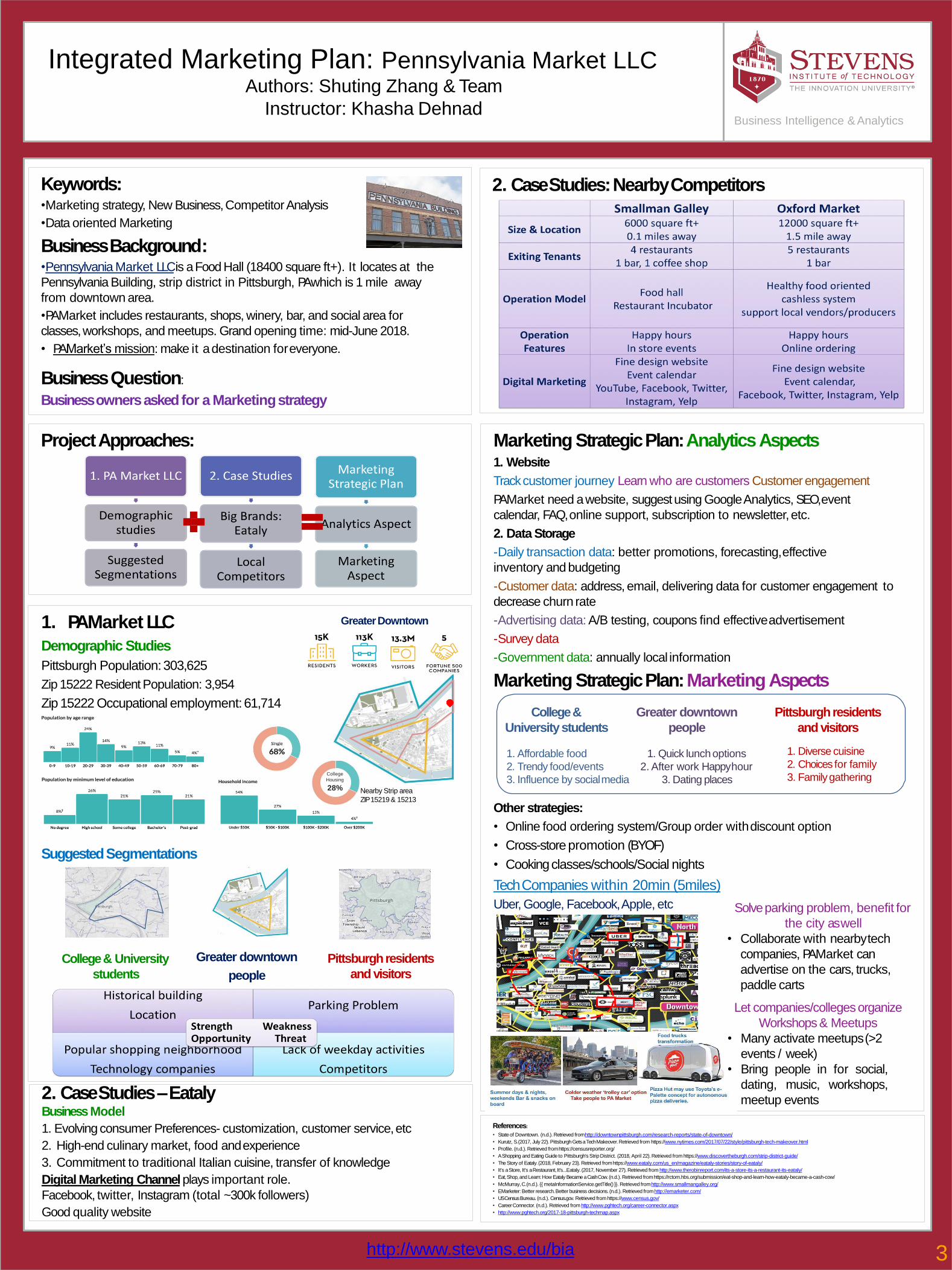
Business Background:•Pennsylvania Market LLCis a Food Hall (18400 square ft+). It locates at the
Pennsylvania Building, strip district in Pittsburgh, PA which is 1 mile away
from downtown area.
•PA Market includes restaurants, shops, winery, bar, and social area for
classes, workshops, and meetups. Grand opening time: mid-June 2018.
• PA Market’s mission: make it a destination foreveryone.
BusinessQuestion:
Business owners asked for a Marketingstrategy
1. PA Market LLC
Demographic Studies
Pittsburgh Population:303,625
Zip 15222 Resident Population: 3,954
Zip 15222 Occupational employment:61,714
SuggestedSegmentations
2. Case Studies –EatalyBusinessModel
1. Evolving consumer Preferences- customization, customer service,etc
2. High-end culinary market, food andexperience
3. Commitment to traditional Italian cuisine, transfer of knowledge
Digital Marketing Channelplays important role.
Facebook, twitter, Instagram (total ~300k followers)
Good quality website
2. Case Studies: NearbyCompetitors
Marketing Strategic Plan: AnalyticsAspects1. Website
Track customer journey Learn who are customers Customer engagement
PA Market need a website, suggest using Google Analytics, SEO, event
calendar, FAQ, online support, subscription to newsletter,etc.
2. Data Storage
-Daily transaction data: better promotions, forecasting,effective
inventory and budgeting
-Customer data: address, email, delivering data for customer engagement to
decrease churn rate
-Advertising data: A/B testing, coupons find effectiveadvertisement
-Survey data
-Government data: annually local information
Marketing Strategic Plan: Marketing Aspects
Other strategies:
• Online food ordering system/Group order withdiscount option
• Cross-store promotion (BYOF)
• Cooking classes/schools/Social nights
Tech Companies within 20min (5miles)
Uber, Google, Facebook, Apple, etc
References:
• State of Downtown. (n.d.). Retrieved fromhttp://downtownpittsburgh.com/research-reports/state-of-downtown/
• Kurutz, S. (2017, July 22). Pittsburgh Gets a Tech Makeover. Retrieved from https://www.nytimes.com/2017/07/22/style/pittsburgh-tech-makeover.html
• Profile. (n.d.). Retrieved fromhttps://censusreporter.org/
• A Shopping and Eating Guide to Pittsburgh's Strip District. (2018, April 22). Retrieved from https://www.discovertheburgh.com/strip-district-guide/
• The Story of Eataly. (2018, February 23). Retrieved fromhttps://www.eataly.com/us_en/magazine/eataly-stories/story-of-eataly/
• It's a Store, It's a Restaurant, It's...Eataly. (2017, November 27). Retrieved from http://www.therobinreport.com/its-a-store-its-a-restaurant-its-eataly/
• Eat, Shop, and Learn: How Eataly Became a Cash Cow. (n.d.). Retrieved fromhttps://rctom.hbs.org/submission/eat-shop-and-learn-how-eataly-became-a-cash-cow/
• McMurray, C. (n.d.). {{ metaInformationService.getTitle() }}. Retrieved fromhttp://www.smallmangalley.org/
• EMarketer: Better research. Better business decisions. (n.d.). Retrieved from http://emarketer.com/
• US Census Bureau. (n.d.). Census.gov. Retrieved from https://www.census.gov/
• Career Connector. (n.d.). Retrieved from http://www.pghtech.org/career-connector.aspx
• http://www.pghtech.org/2017-18-pittsburgh-techmap.aspx
ProjectApproaches:
GreaterDowntown
College
Housing
28% Nearby Strip area
ZIP 15219 & 15213
Pittsburgh residents
and visitors
Greater downtown
people
College & University
students
Pittsburgh residents
and visitors
Greater downtown
people
College &
Universitystudents
1. Diverse cuisine
2. Choices for family
3. Familygathering
1. Quick lunchoptions
2. After work Happyhour
3. Dating places
1. Affordable food
2. Trendy food/events
3. Influence by socialmedia
Solve parking problem, benefit for
the city aswell
• Collaborate with nearbytech
companies, PA Market can
advertise on the cars, trucks,
paddle carts
Let companies/collegesorganize
Workshops & Meetups
• Many activate meetups(>2
events / week)
• Bring people in for social,
dating, music, workshops,
meetup events
http://www.stevens.edu/bia 3
Wealth Management BranchPredictionAuthors: Shuting Zhang, Harsh Kava
Instructors: Prof. David Belanger, Prof. Edward Stohr, Prof. KhashaDehnad
Keywords:• Python, Tableau
• Supervised Learning
• Hybrid Data ScienceModeling
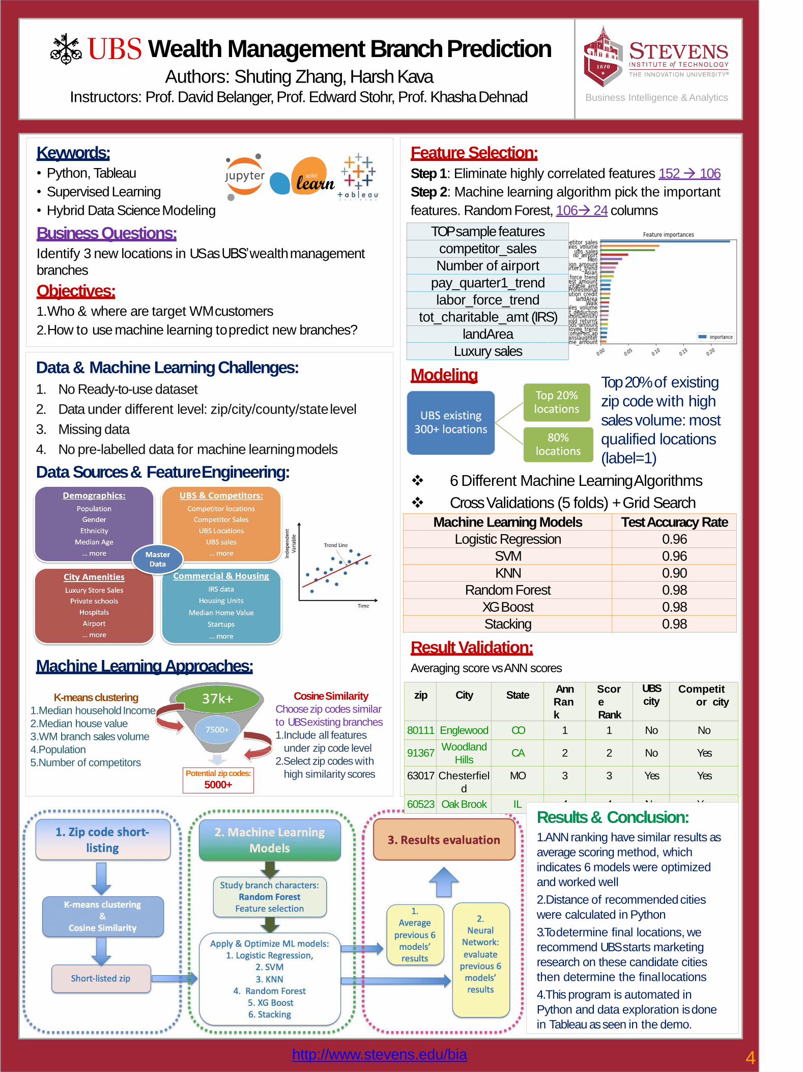
BusinessQuestions:Identify 3 new locations in US as UBS’ wealthmanagement
branches
Objectives:1.Who & where are target WMcustomers
2.How to use machine learning topredict new branches?
Data & Machine LearningChallenges:
1. No Ready-to-use dataset
2. Data under different level: zip/city/county/statelevel
3. Missing data
4. No pre-labelled data for machine learningmodels
Data Sources & FeatureEngineering:
Machine LearningApproaches:
Business Intelligence & Analytics
Feature Selection:Step 1: Eliminate highly correlated features 152→ 106
Step 2: Machine learning algorithm pick the important
features. Random Forest, 106→ 24 columns
Modeling
❖ 6 Different Machine LearningAlgorithms
❖ Cross Validations (5 folds) + Grid Search
Result Validation:Averaging score vs ANN scores
Potential zipcodes:
5000+
K-means clustering
1.Median household Income
2.Median house value
3.WM branch sales volume
4.Population
5.Number of competitors
Cosine Similarity
Choose zip codes similar
to UBS existing branches
1.Include all features
under zip code level
2.Select zip codeswith
high similarity scores
TOP sample features
competitor_sales
Number of airport
pay_quarter1_trend
labor_force_trend
tot_charitable_amt (IRS)
landArea
Luxury sales
Machine Learning Models Test Accuracy Rate
Logistic Regression 0.96
SVM 0.96
KNN 0.90
Random Forest 0.98
XGBoost 0.98
Stacking 0.98
http://www.stevens.edu/bia 4
Top 20% of existing
zip code with high
sales volume: most
qualified locations
(label=1)
zip City StateAnn
Ran
k
Scor
e
Rank
UBS
cityCompetit
or city
80111 Englewood CO 1 1 No No
91367Woodland
HillsCA 2 2 No Yes
63017 Chesterfiel
d
MO 3 3 Yes Yes
60523 OakBrook IL 4 4 No Yes
Results & Conclusion:1.ANN ranking have similar results as
average scoring method, which
indicates 6 models were optimized
and worked well
2.Distance of recommendedcities
were calculated in Python
3.To determine final locations, we
recommend UBS starts marketing
research on these candidate cities
then determine the finallocations
4.This program is automated in
Python and data exploration isdone
in Tableau as seen in the demo.
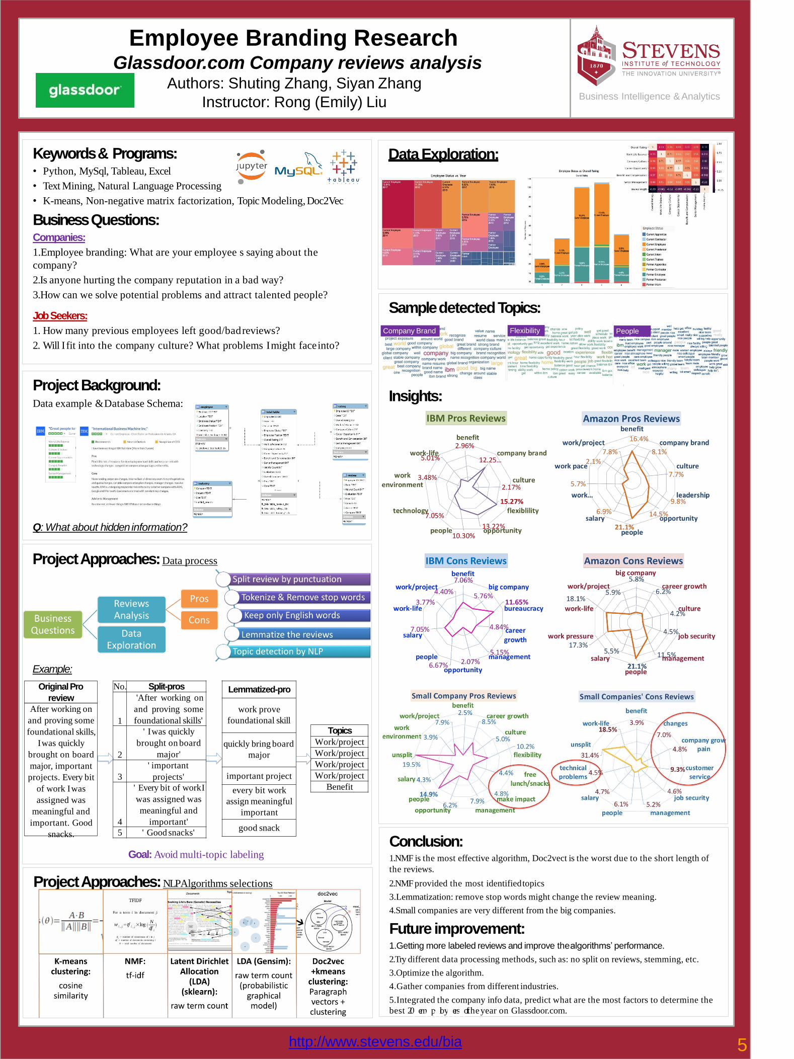
Employee Branding ResearchGlassdoor.com Company reviews analysis
Authors: Shuting Zhang, Siyan Zhang
Instructor: Rong (Emily) LiuBusiness Intelligence & Analytics
Sample detectedTopics:
Insights:
Keywords & Programs:• Python, MySql, Tableau, Excel
• Text Mining, Natural Language Processing
• K-means, Non-negative matrix factorization, Topic Modeling, Doc2Vec
BusinessQuestions:Companies:
1.Employee branding: What are your employee s saying about the
company?
2.Is anyone hurting the company reputation in a bad way?
3.How can we solve potential problems and attract talented people?
JobSeekers:
1. How many previous employees left good/badreviews?
2. Will I fit into the company culture? What problems I might faceinto?
Project Background:Data example & Database Schema:
Conclusion:1.NMF is the most effective algorithm, Doc2vect is the worst due to the short length of
the reviews.
2.NMF provided the most identifiedtopics
3.Lemmatization: remove stop words might change the review meaning.
4.Small companies are very different from the big companies.
Future improvement:1.Getting more labeled reviews and improve thealgorithms’ performance.
2.Try different data processing methods, such as: no split on reviews, stemming, etc.
3.Optimize the algorithm.
4.Gather companies from different industries.
5.Integrated the company info data, predict what are the most factors to determine the
best 20eemdpulo/yberisaof theyear on Glassdoor.com.
Q: What about hidden information?
Project Approaches: Data process
Example:
Goal: Avoid multi-topic labeling
Original Pro
review
After working on
and proving some
foundational skills,
I was quickly
brought on board
major, important
projects. Every bit
of work I was
assigned was
meaningful and
important. Good
snacks.
No. Split-pros
1
'After working on
and proving some
foundational skills'
2
' I was quickly
brought on board
major'
3
' important
projects'
4
' Every bit of workI
was assigned was
meaningful and
important'
5 ' Good snacks'
Lemmatized-pro
work prove
foundational skill
quickly bring board
major
important project
every bit work
assign meaningful
important
good snack
Topics
Work/project
Work/project
Work/project
Work/project
Benefit
Project Approaches: NLP Algorithms selections
Data Exploration:
Flexibility PeopleCompany Brand
http://www.stevens.edu/bia 5

Biometric Data Analysis over 120 years forOlympic
AthletesAuthors: Yanzhao Liang, Zhihao Zhang, Hao Xu, Yingjian Song
Instructor: Alkiviadis Vazacopoulos
Age AnalysisThe two figures contain the athlete's age and gender data. By
analyzing these data we canfind:
1. What is the age of the athletes? What age of athletes is
more suitable for the Olympics?
2. What is the best age for male athletes? What is the best
age for female atheletes?
IntroductionWe have selected data for all athletes in the history of the
Olympic Games. These data contain:
1. Data for athletes in allcountries.
2. Age, height, weight, championship status, etc. of all athletes.
3. The order of athletes is ranked by last name.
Gold Medals In Each CountryFrom the figure we can see which countries are stronger,
which countries are better at the Summer Olympics, and
which countries are better at the Winter Olympics.
The figure above show the gold medals for the Summer
Olympics. The figure below shows the gold medal for the
Winter Olympics.
Summer Olympics
Winter Olympics
Number Of SportsThe figure depicts the changes in sports as the year progresses.
One of the sharp declines is due to war, and other years are
steadily increasing.
Height/Weight AnalysisIn this section, we analyze the relationship between the
height and weight of the athlete and the gold medal. In
the figure on the left, the darker part represents the
height of the athlete and the weight.
Business Intelligence & Analytics
http://www.stevens.edu/bia 6
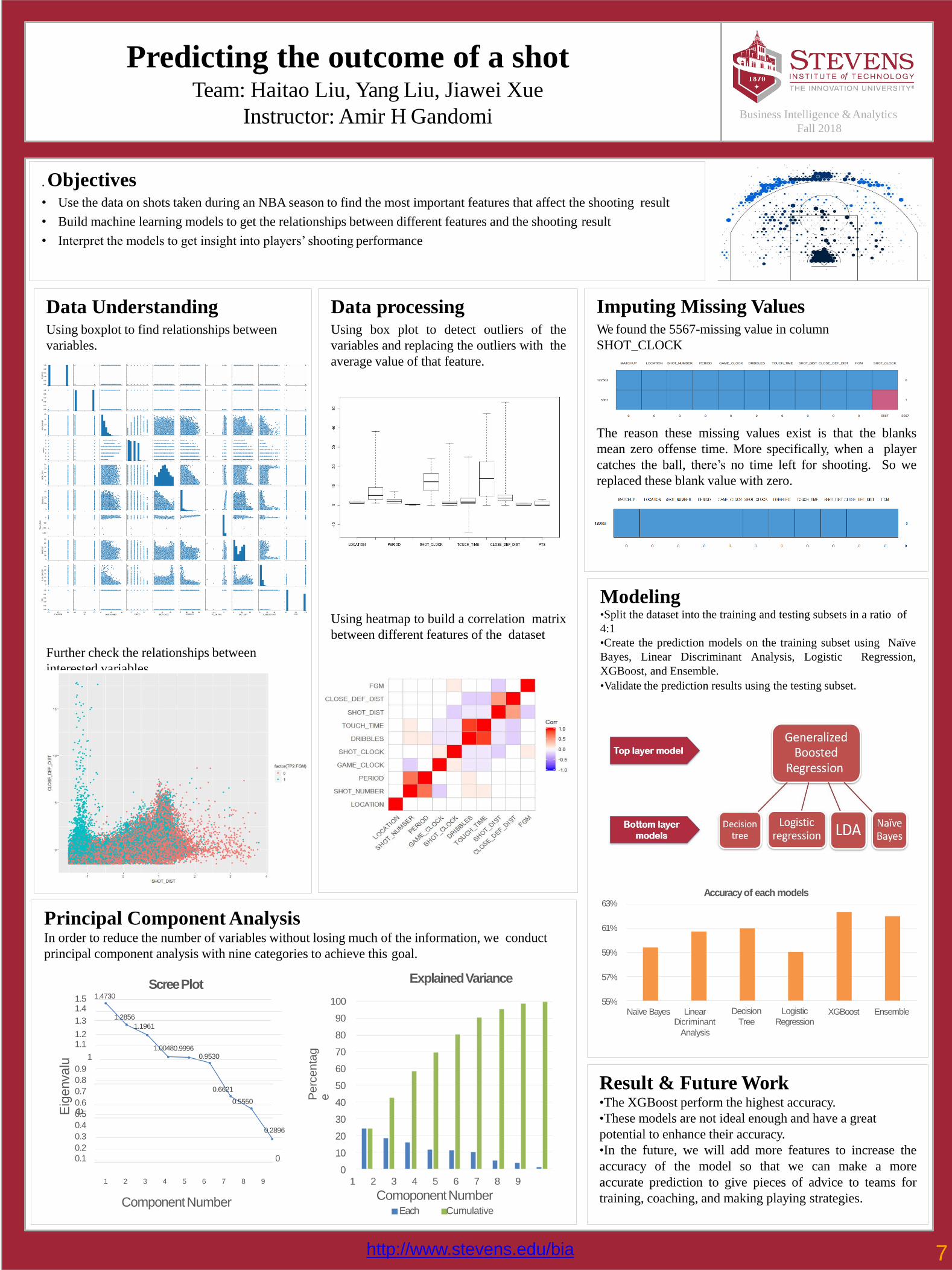
Predicting the outcome of a shotTeam: Haitao Liu, Yang Liu, Jiawei Xue
Instructor: Amir H Gandomi Business Intelligence &Analytics
Fall 2018
. Objectives• Use the data on shots taken during an NBA season to find the most important features that affect the shooting result
• Build machine learning models to get the relationships between different features and the shooting result
• Interpret the models to get insight into players’ shooting performance
Data UnderstandingUsing boxplot to find relationships between
variables.
Further check the relationships between
interested variables
Eig
envalu
e
ComponentNumber
ScreePlot1.5 1.4730
1.4
1.31.2856
1.1961
1.21.1
1.00480.9996
1 0.9530
0.9
0.8
0.7 0.6621
0.6 0.5550
0.5
0.40.2896
0.3
0.2
0.1 0
100
90
80
70
60
50
40
30
20
10
01 2 3 4 5 6 7 8 9 1 2 3 4 5 6 7 8 9
Perc
enta
ge
Principal Component AnalysisIn order to reduce the number of variables without losing much of the information, we conduct
principal component analysis with nine categories to achieve this goal.
ExplainedVariance
ComoponentNumberEach Cumulative
Data processingUsing box plot to detect outliers of the
variables and replacing the outliers with the
average value of that feature.
Using heatmap to build a correlation matrix
between different features of the dataset
Imputing Missing ValuesWe found the 5567-missing value in column
SHOT_CLOCK
The reason these missing values exist is that the blanks
mean zero offense time. More specifically, when a player
catches the ball, there’s no time left for shooting. So we
replaced these blank value with zero.
Modeling•Split the dataset into the training and testing subsets in a ratio of
4:1
•Create the prediction models on the training subset using Naïve
Bayes, Linear Discriminant Analysis, Logistic Regression,
XGBoost, and Ensemble.
•Validate the prediction results using the testing subset.
Result & Future Work•The XGBoost perform the highest accuracy.
•These models are not ideal enough and have a great
potential to enhance their accuracy.
•In the future, we will add more features to increase the
accuracy of the model so that we can make a more
accurate prediction to give pieces of advice to teams for
training, coaching, and making playing strategies.
63%
61%
59%
57%
55%
http://www.stevens.edu/bia 7
Naïve Bayes LinearDicriminant
Analysis
Decision
Tree
Logistic
RegressionXGBoost Ensemble
Accuracy of each models
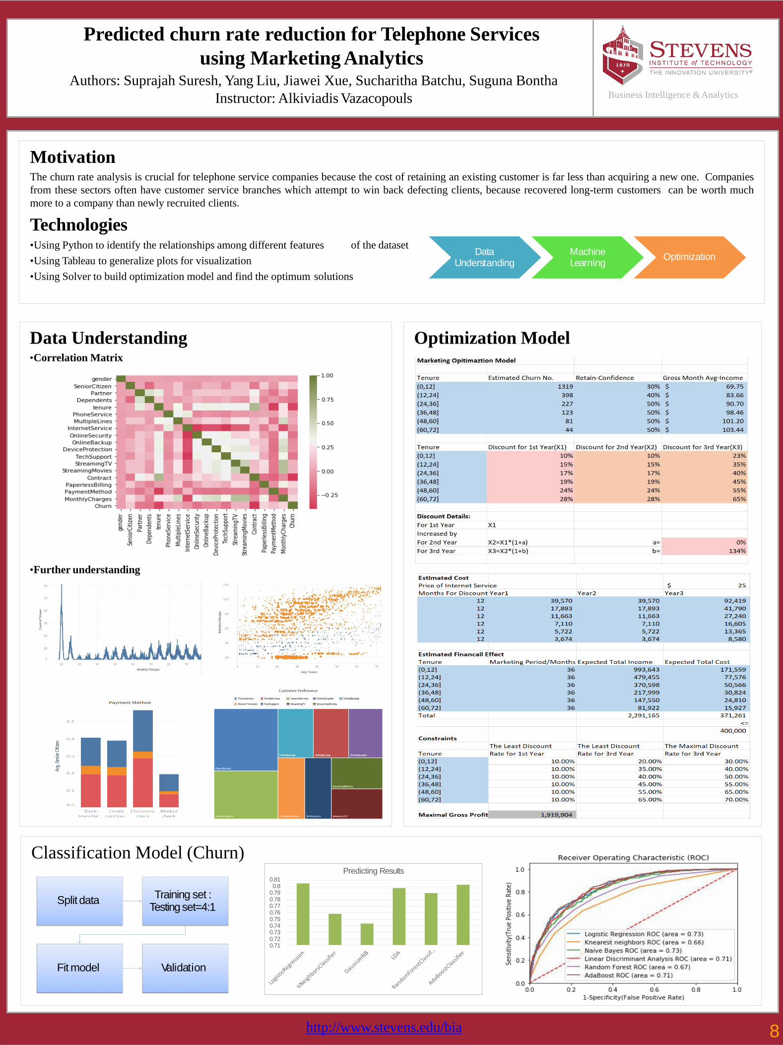
Predicted churn rate reduction for Telephone Services
using Marketing AnalyticsAuthors: Suprajah Suresh, Yang Liu, Jiawei Xue, Sucharitha Batchu, Suguna Bontha
Instructor: Alkiviadis Vazacopouls
MotivationThe churn rate analysis is crucial for telephone service companies because the cost of retaining an existing customer is far less than acquiring a new one. Companies
from these sectors often have customer service branches which attempt to win back defecting clients, because recovered long-term customers can be worth much
more to a company than newly recruited clients.
Technologiesof the dataset•Using Python to identify the relationships among different features
•Using Tableau to generalize plots for visualization
•Using Solver to build optimization model and find the optimum solutions
Data Understanding•Correlation Matrix
•Further understanding
Classification Model (Churn)
Business Intelligence &Analytics
Optimization Model
Data Understanding
Machine Learning
Optimization
Predicting Results0.810.8
0.790.780.770.760.750.740.730.720.71
Split dataTraining set :
Testing set=4:1
Fit model Validation
http://www.stevens.edu/bia 8

Budget allocation optimization for natural
disaster preparationAuthors: Nifan Yuan, Jiahao Shi, Lianhong Deng, Yuxuan Gu , Haohan Hu
Instructor: Alkis Vazacopoulos
Subject to:
Motivation -- Why we choose this topic:
During 1997 and 2017, The economic damages of natural disasters are getting bigger andbigger;
The United States ranked the first place of economic losses all over the world.
Technology:• We use R for generating the result NLP files of the
mathematical models and the visualization through
GGPLOT.
• We use NLP Solver for solving the optimization models.
Estimation of the future:• The expected trend of natural disasters is showingan
upward trend.
• Economic damage will rise as a share of gross domestic
product (GDP), which provides a measure of the nation’s
ability to pay for thatdamage.
Business Intelligence & Analytics
Current & FutureWork:• Development formulas to build the model to analyze the
past data and choosing the best model to predict the future.
• Seeking more factors and trying to find frequency which
would multiple the formula to make the model better.
• Development a visualization work of the budgetallocated
on the target states.
i
Experiment:P = population
G = GDP of State
E = Elevation of State
b = Budget
i
i
F (D) = P*G
E *(1+ b ) ^ 2
Constraint:n
i
i=1
b 10000M
ib 500M
n
Min F (D)i=1
i
State GDP Pop Feet Bud DF
Texas 2,056,072.41
2,056,072.41
1,700.00
14,812.24 6.34
Oklahoma 223,759.01 223,759.01 1,300.00
500.00 1.27
Ohio 728,350.81 728,350.81 850.00 7,415.40 4.05
Newyork 1,792,387.61
1,792,387.61
1,000.00
16,389.61 7.02
Missouri 342,407.18 342,407.18 800.00 2,670.47 2.49
Mississipi 126,029.20 126,029.20 300.00 500.00 1.75
Lousiana 284,111.46 284,111.46 100.00 8,493.19 4.43
Florida 1,135,263.31
1,135,263.31
100.00 29,748.68 10.67
California 3,268,754.11
3,268,754.11
2,900.00
17,380.22 7.36
Alabama 240,552.98 240,552.98 500.00 2,090.19 2.30
100,000.00
Minsubject 47.69
Top 10 states selected:Texas
Oklahoma
Ohio
New York
Missouri
Mississippi
Louisiana
Florida
California
Alabama
http://www.stevens.edu/bia 9
Revenue and Cost Optimization for a Clothing
Supply ChainAuthors: Weifeng Li, Liran Zhang, Mingxin Zheng, Zeyu Shao
Instructor : Alkiviadis Vazacopoulus
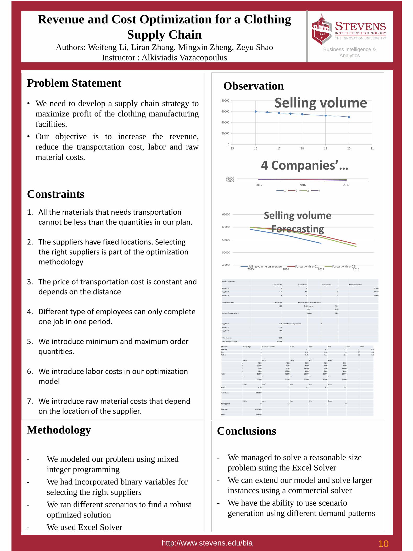
Observation
Methodology
- We modeled our problem using mixed
integer programming
- We had incorporated binary variables for
selecting the right suppliers
- We ran different scenarios to find a robust
optimized solution
- We used Excel Solver
Business Intelligence &
Analytics
http://www.stevens.edu/bia
Problem Statement
• We need to develop a supply chain strategy to
maximize profit of the clothing manufacturing
facilities.
• Our objective is to increase the revenue,
reduce the transportation cost, labor and raw
material costs.
Constraints
1. All the materials that needs transportation cannot be less than the quantities in our plan.
2. The suppliers have fixed locations. Selecting the right suppliers is part of the optimization methodology
3. The price of transportation cost is constant and depends on the distance
4. Different type of employees can only complete one job in one period.
5. We introduce minimum and maximum order quantities.
6. We introduce labor costs in our optimization model
7. We introduce raw material costs that depend on the location of the supplier.
Conclusions
- We managed to solve a reasonable size
problem suing the Excel Solver
- We can extend our model and solve larger
instances using a commercial solver
- We have the ability to use scenario
generation using different demand patterns
0
20000
40000
60000
80000
15 16 17 18 19 20 21
Selling volume
4500065000
2015 2016 2017
4 Companies’ …
1 2 3 4
45000
50000
55000
60000
65000
2015 2016 2017 2018
Selling volume Forecasting
Selling volume on average Forcast with a=0.1 Forcast with a=0.5
Supplier's location
X-coordinate Y-coordinate Vans needed Materials needed
Supplier 1 0 0 25 50000
Supplier 2 2.1 2.5 9 22500
Supplier 3 5 0 14 24500
Factory's location X-coordinate Y-coordinateEach Van's capacity
2.16 1.42 Drapery 2000
Fur 2500
Distance from suppliers Cotton 1800
Supplier 1 2.59 Trasportation fee(/van/km) 8
Supplier 2 1.08
Supplier 3 3.17
Total distance 684
Total transportation cost 94116
Material Price($/kg) Required quantity Shirts Jeans Hats Belts Shoes
Drapery 3 0.1 0.4 0.1 0.1 0.4
Fur 15 0.02 0.05 0 0.3 0.4
Cotton 1 0.06 0.15 0.1 0.1 0.2
Shirts Jeans Coats Belts Shoes
1 4000 4000 4000 4000 4000
2 38000 4000 4000 4000 4000
3 4000 4000 18000 4000 18000
4 4000 58000 4000 8000 4000
Total 50000 70000 30000 20000 30000
<= <= <= <= <=
50000 70000 30000 20000 30000
Shirts Jeans Hats Belts Shoes
Costs 0.66 2.1 0.4 4.9 7.4
Total Costs 512000
Shirts Jeans Hats Belts Shoes
Selling price 20 10 5 15 10
Revenue 2450000
Profit 1938000
10
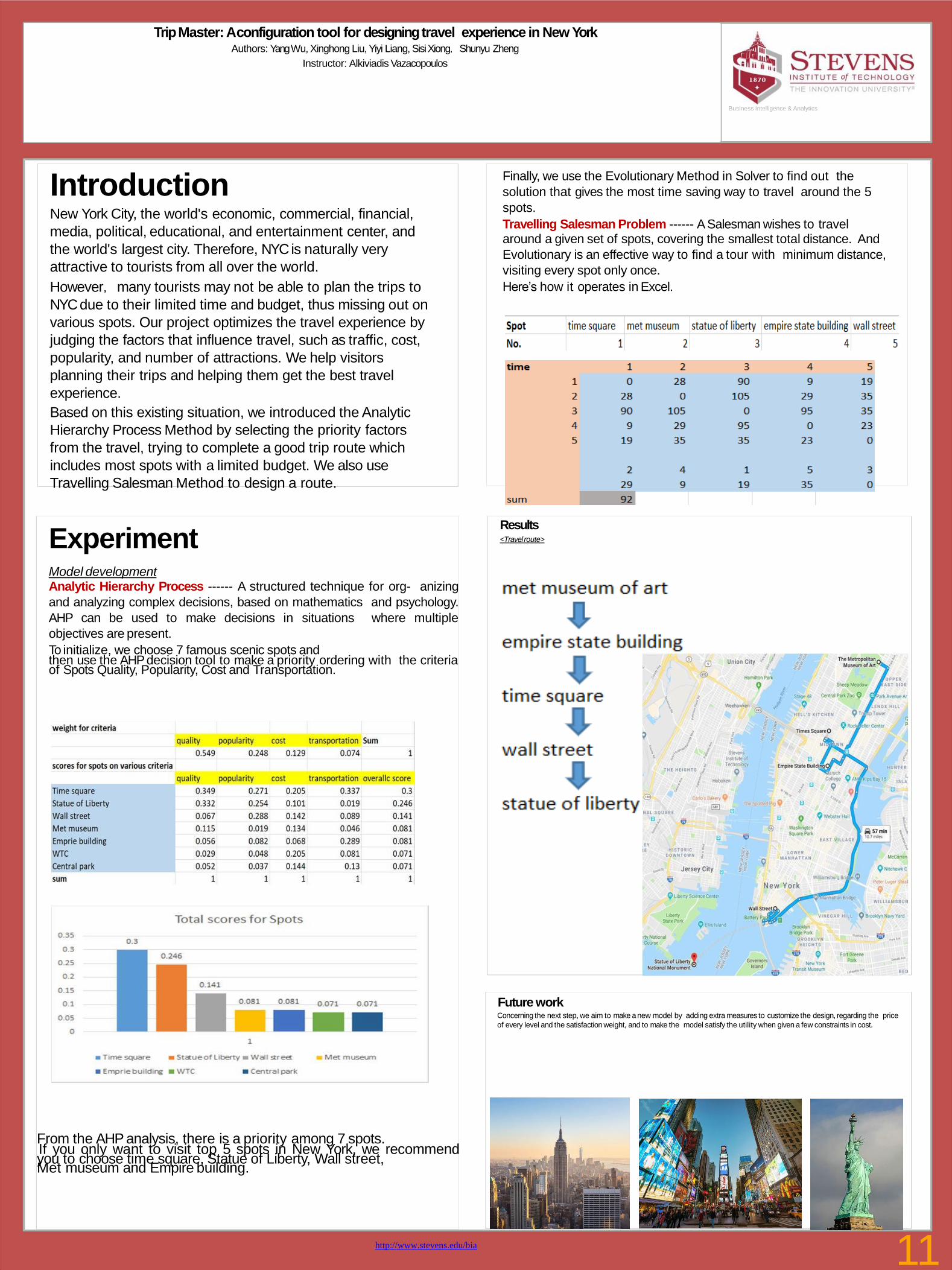
Trip Master: A configuration tool for designing travel experience in New YorkAuthors: Yang Wu, Xinghong Liu, Yiyi Liang, Sisi Xiong,Shunyu Zheng
Instructor: Alkiviadis Vazacopoulos
Results<Travelroute>
IntroductionNew York City, the world's economic, commercial, financial,
media, political, educational, and entertainment center, and
the world's largest city. Therefore, NYC is naturally very
attractive to tourists from all over the world.
However,many tourists may not be able to plan the trips to
NYCdue to their limited time and budget, thus missing out on
various spots. Our project optimizes the travel experience by
judging the factors that influence travel, such as traffic, cost,
popularity, and number of attractions. We help visitors
planning their trips and helping them get the best travel
experience.
Based on this existing situation, we introduced the Analytic
Hierarchy Process Method by selecting the priority factors
from the travel, trying to complete a good trip route which
includes most spots with a limited budget. We also use
Travelling Salesman Method to design a route.
ExperimentModel developmentAnalytic Hierarchy Process ------ A structured technique for org- anizing
and analyzing complex decisions, based on mathematics and psychology.
AHP can be used to make decisions in situations where multiple
objectives are present.
To initialize, we choose 7 famous scenic spots andthen use the AHP decision tool to make a priority ordering with the criteria of Spots Quality, Popularity, Cost and Transportation.
From the AHP analysis, there is a priority among 7 spots.If you only want to visit top 5 spots in New York, we recommendyou to choose time square, Statue of Liberty, Wall street,Met museum and Empire building.
Business Intelligence & Analytics
Finally, we use the Evolutionary Method in Solver to find out the
solution that gives the most time saving way to travel around the 5
spots.
Travelling Salesman Problem ------ A Salesman wishes to travelaround a given set of spots, covering the smallest total distance. And
Evolutionary is an effective way to find a tour with minimum distance,
visiting every spot only once.
Here’s how it operates in Excel.
Future workConcerning the next step, we aim to make a new model by adding extra measures to customize the design, regarding the price
of every level and the satisfaction weight, and to make the model satisfy the utility when given a few constraints in cost.
11http://www.stevens.edu/bia
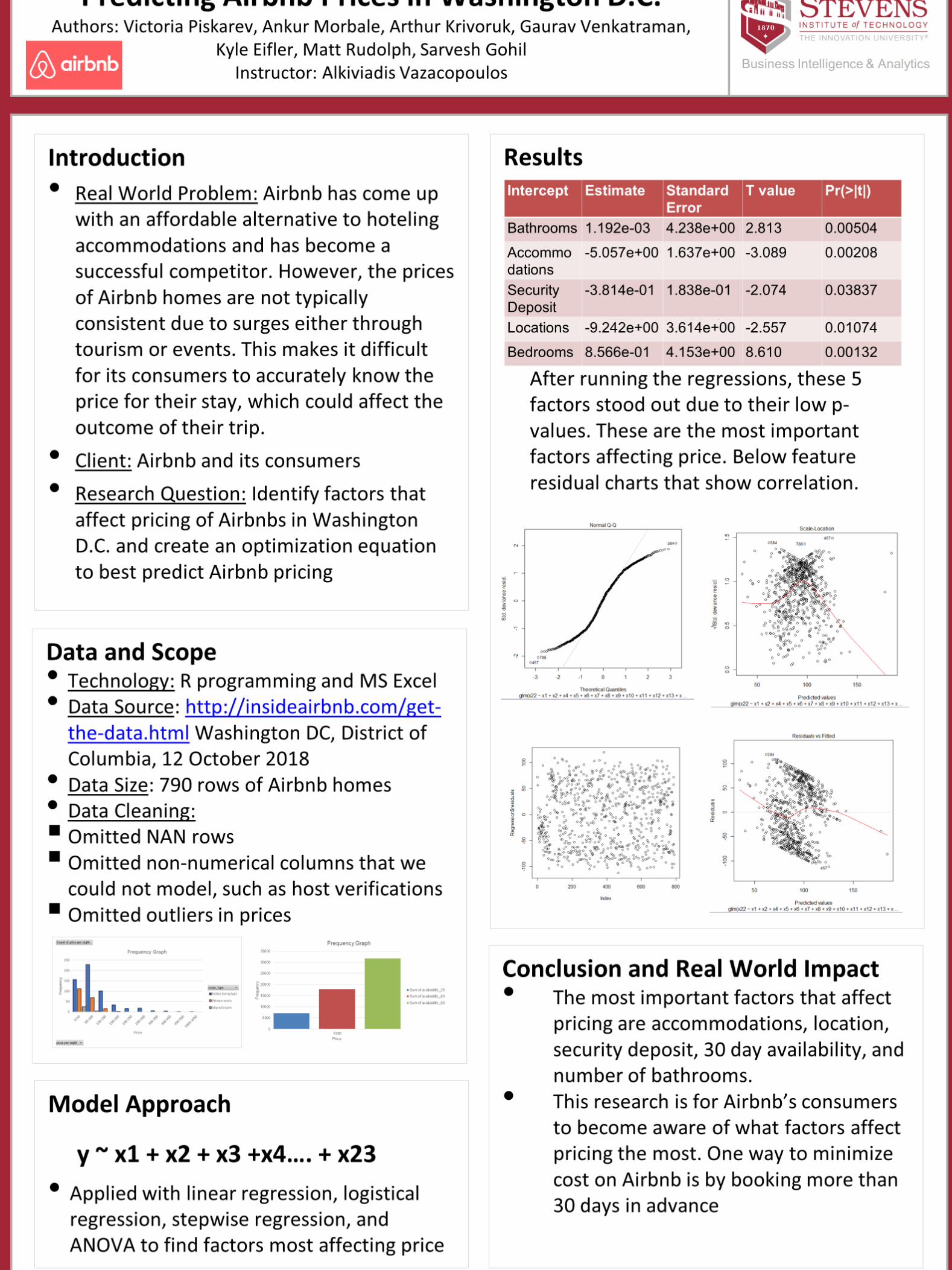
After running the regressions, these 5
factors stood out due to their low p-
values. These are the most important
factors affecting price. Below feature
residual charts that show correlation.
for its consumers to accurately know the
price for their stay, which could affect the
outcome of their trip.
• Client: Airbnb and its consumers
• Research Question: Identify factors that
affect pricing of Airbnbs in Washington
D.C. and create an optimization equation
to best predict Airbnb pricing
Real World Problem: Airbnb has come up
with an affordable alternative to hoteling
Intercept Estimate Standard T value Pr(>|t|)
Error
Accommo -5.057e+00 1.637e+00 -3.089 0.00208
successful competitor. However, the prices dations
of Airbnb homes are not typically Security -3.814e-01 1.838e-01 -2.074 0.03837
consistent due to surges either throughDeposit
Locations -9.242e+00 3.614e+00 -2.557 0.01074
tourism or events. This makes it difficult Bedrooms 8.566e-01 4.153e+00 8.610 0.00132
Predicting Airbnb Prices in Washington D.C.Authors: Victoria Piskarev, Ankur Morbale, Arthur Krivoruk, Gaurav Venkatraman, Kyle Eifler, Matt Rudolph, Sarvesh Gohil
Instructor: Alkiviadis VazacopoulosBusiness Intelligence & Analytics
Data and Scope• Technology: R programming and MS Excel
• Data Source: http://insideairbnb.com/get-the-data.html Washington DC, District of Columbia, 12 October 2018
• Data Size: 790 rows of Airbnb homes
• Data Cleaning:
▪ Omitted NAN rows
▪ Omitted non-numerical columns that we could not model, such as host verifications
▪ Omitted outliers in prices
ResultsIntroduction
•
accommodations and has become aBathrooms 1.192e-03 4.238e+00 2.813 0.00504
Conclusion and Real World Impact• The most important factors that affect pricing are accommodations, location, security
deposit, 30 day availability, and
number of bathrooms.• This research is for Airbnb’s consumers to become aware of what factorsaffect pricing
the most. One way to minimize cost on Airbnb is by booking more than
30 days in advance
ModelApproach
y ~ x1 + x2 + x3 +x4…. + x23
• Applied with linear regression, logistical regression, stepwise regression, and ANOVA to find
factors most affecting price
0
5000
10000
15000
20000
25000
30000
Fre
quency
Total
Price
Frequency Graph
35000
Sum of availability_30 Sum of availability_60 Sum
ofavailability_90
http://www.stevens.edu/bia
12
Acknowledgments:
allowing me to pursue a research a r e a I wa s v e r y interested in
whi l e providing all the knowledge and expereince he had in the
field. I would also like to thank Steven’s for providing the opportunity
to experience the research field firsthand.
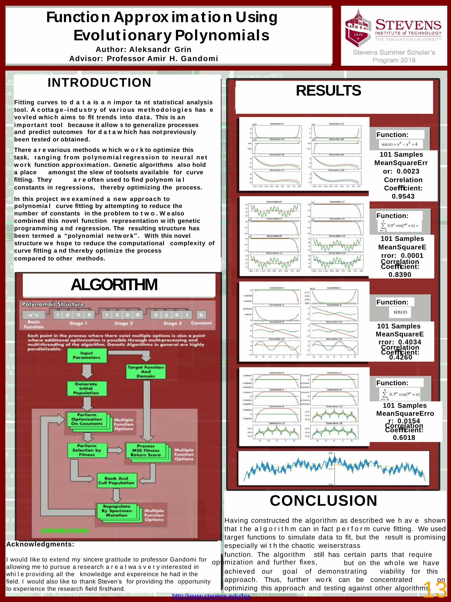
RESULTS
Function:
Function:
101 Samples MeanSquareError: 0.4034CorrelationCoefficient:
0.4260
101 Samples
MeanSquareE
rror: 0.0001CorrelationCoefficient:
0.8390
Function:
101 Samples
MeanSquareErr
or: 0.0023
Correlation
Coefficient:
0.9543
Function:
101 SamplesMeanSquareErro
r: 0.0154CorrelationCoefficient:
0.6018
Function Approx imat ion Using
Evolut ionary PolynomialsAuthor: Aleksandr Grin
Advisor: Professor Amir H. Gandomi
INTRODUCTION
Fitting curves to d a t a is a n impor ta nt statistical analysis
tool. A c otta g e - i nd u s tr y of va r i o us m e t h o d o l o g i e s has e
vo vled whic h aims to fit trends into data. This is an
important tool because it allow s to generalize processesand predict outcomes for d a t a w hich has not previously
been tested or obtained.
There a r e various methods w hich w o r k to optimize this
task, ranging from polynomial regression to neural ne t
w ork function approximation. Genetic algorithms also hold
a place amongst the slew of toolsets available for curve
fitting. They a r e often used to find polynom ia l
constants in regressions, thereby optimizing the process.
In this project w e examined a new appr oa ch topolynomia l curve fitting by attempting to reduce the
number of constants in the problem to t w o . W e also
combined this novel function representation w ith genetic
programming a nd regression. The resulting structure has
been termed a “polynomial netw or k” . With this novel
structure w e hope to reduce the computational complexity of
curve fitting a nd thereby optimize the process
compared to other methods.
CONCLUSIONHaving constructed the algorithm as described we h av e shown
that t he a l g o r i t h m can in fact p e r f o r m curve fitting. We used
target functions to simulate data to fit, but the result is promising
especially wi t h the chaotic weiserstrass
function. The algorithm still has certain parts that requireI would like to extend my sincere gratitude to professor Gandomi for optimization and further fixes, but on the wh ole we have
achieved our goal of demonstrating viability for this
approach. Thus, further wo rk can be concentrated on
optimizing this approach and testing against other algorithms.
ALGORITHM
13http://www.stevens.edu/bia
CorrelatingLong-TermInnovation with Successin
CareerProgressionAdam Coscia
Instructors:Aron Lindberg,Ph.D.,Amir Gandomi,Ph.D.
Motivation• Successful individuals and
businesses in all fields
explore new innovations and/or exploit
successful ones.
• Intervals of strategy exploration and
exploitation may affect long-term success,
independent of career type and field.
• Developing long-term innovation models to
maximize career success is the goal!
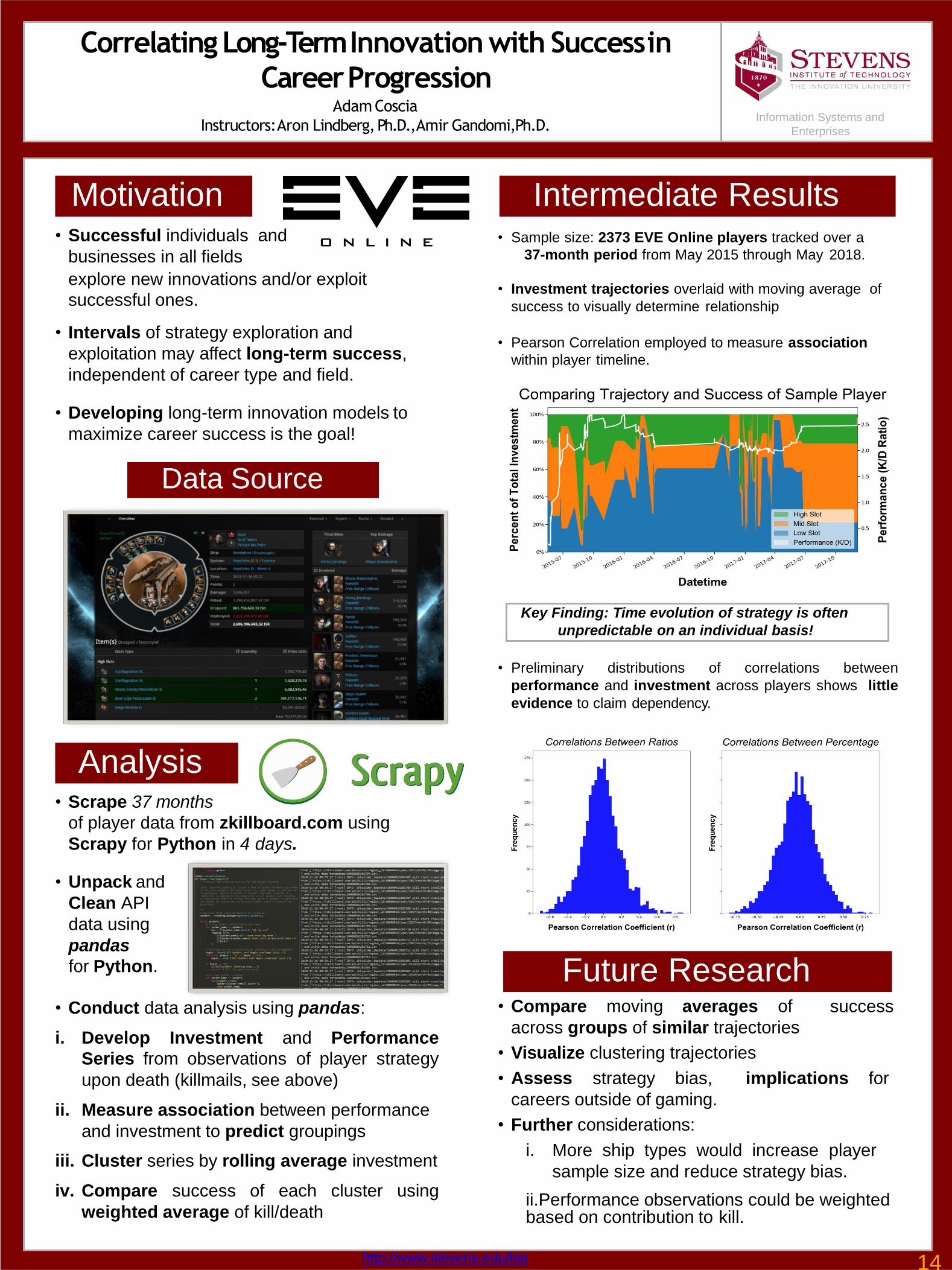
Intermediate Results• Sample size: 2373 EVE Online players tracked over a
37-month period from May 2015 through May 2018.
• Investment trajectories overlaid with moving average of
success to visually determine relationship
• Pearson Correlation employed to measure association
within player timeline.
Key Finding: Time evolution of strategy is often
unpredictable on an individual basis!
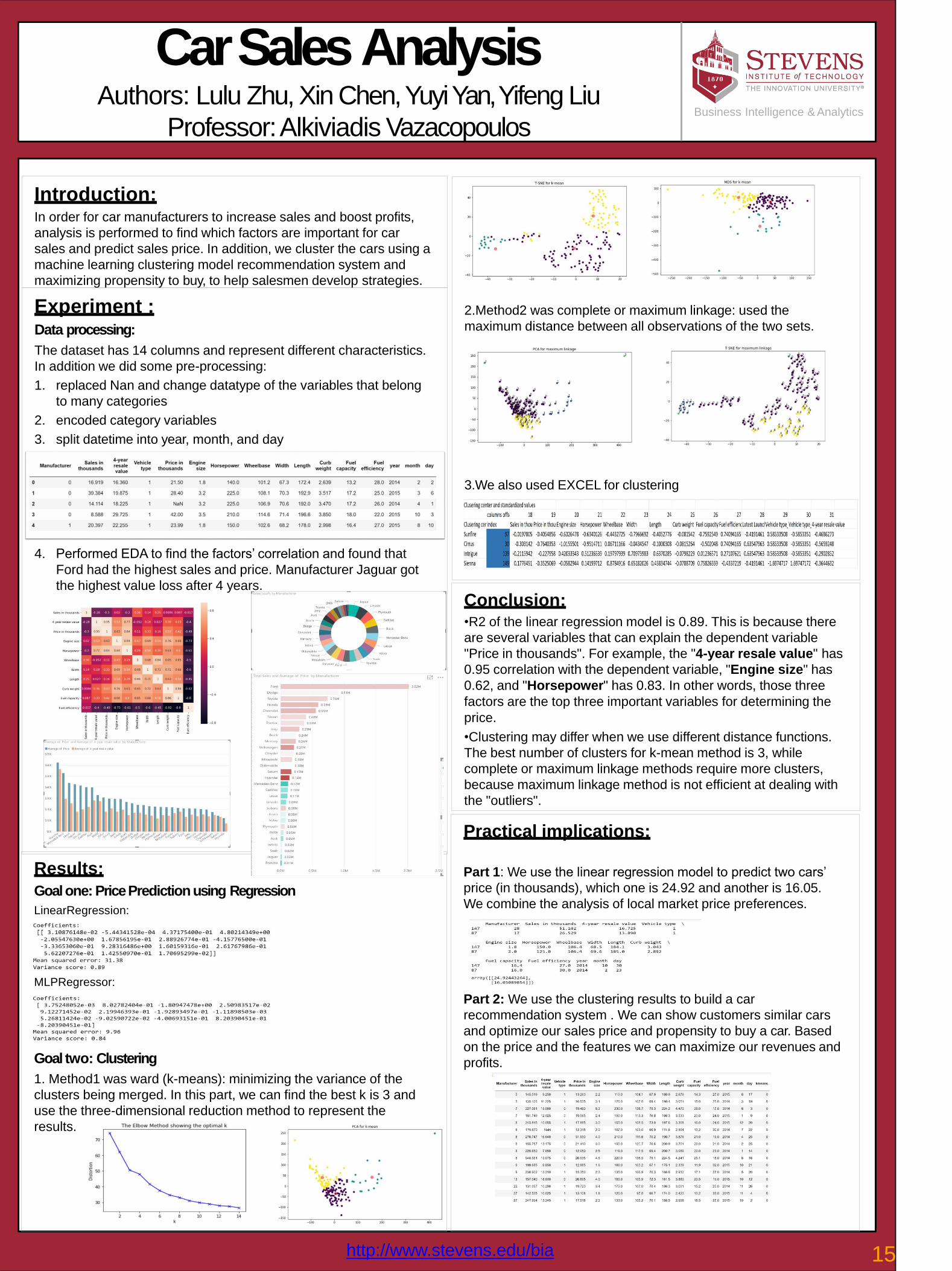
• Preliminary distributions of correlations between
performance and investment across players shows little
evidence to claim dependency.
Analysis• Scrape 37 months
of player data from zkillboard.com using
Scrapy for Python in 4 days.
• Unpack and
Clean API
data using
pandas
for Python.
• Conduct data analysis using pandas:
i. Develop Investment and Performance
Series from observations of player strategy
upon death (killmails, see above)
ii. Measure association between performance
and investment to predict groupings
iii. Cluster series by rolling average investment
iv. Compare success of each cluster using
weighted average of kill/death
Future Researchsuccess• Compare moving averages of
across groups of similar trajectories
• Visualize clustering trajectories
implications for• Assess strategy bias,
careers outside of gaming.
• Further considerations:
i. More ship types would increase player
sample size and reduce strategy bias.
Information Systems and
Enterprises
Data Source
ii.Performance observations could be weighted based on contribution to kill.
http://www.stevens.edu/bia 14
Car SalesAnalysisAuthors: Lulu Zhu, Xin Chen, Yuyi Yan, Yifeng Liu
Professor: Alkiviadis Vazacopoulos
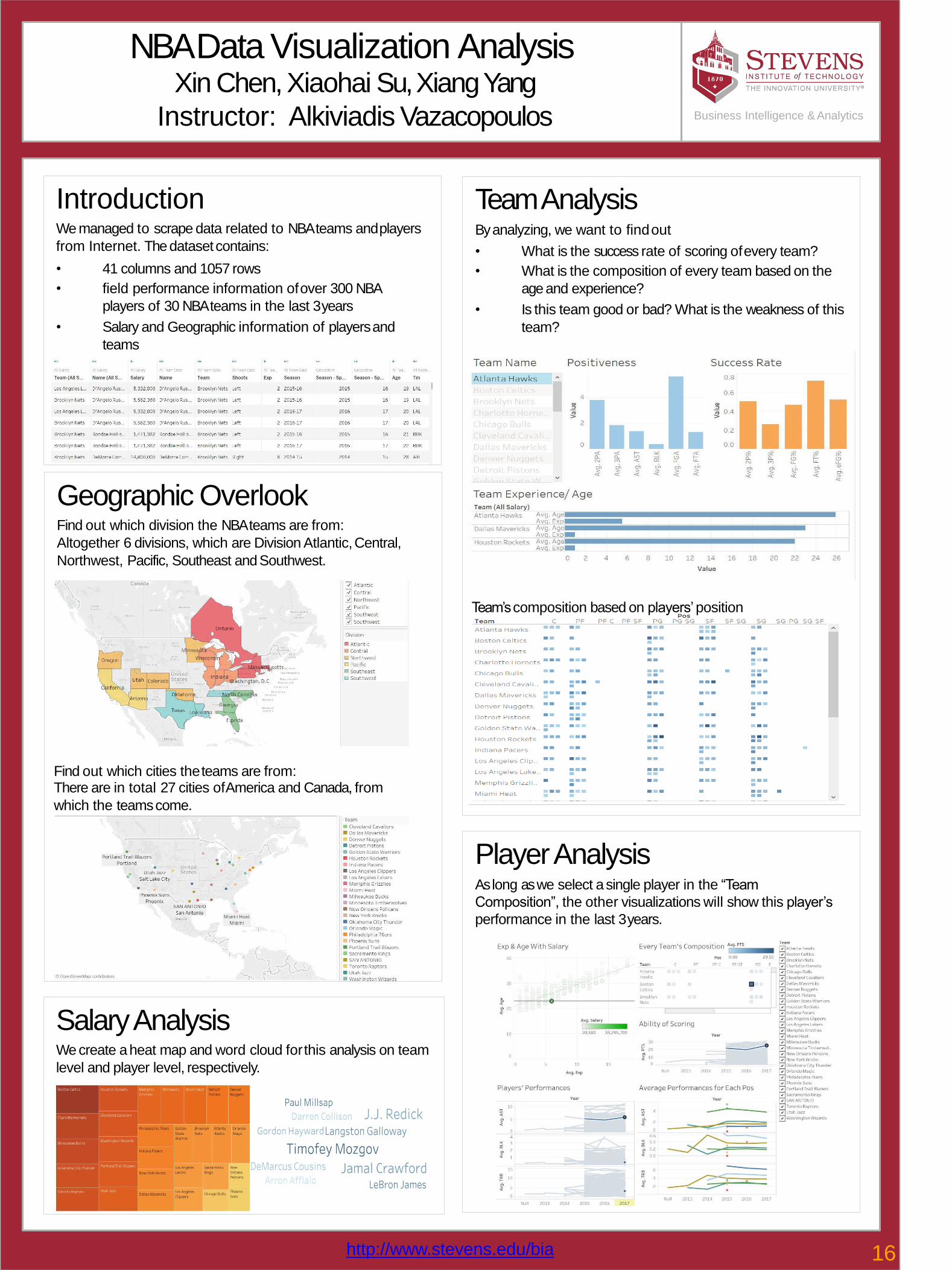
2.Method2 was complete or maximum linkage: used the
maximum distance between all observations of the two sets.
3.We also used EXCEL for clustering
Introduction:In order for car manufacturers to increase sales and boost profits,
analysis is performed to find which factors are important for car
sales and predict sales price. In addition, we cluster the cars using a
machine learning clustering model recommendation system and
maximizing propensity to buy, to help salesmen develop strategies.
Experiment :Data processing:
The dataset has 14 columns and represent different characteristics.
In addition we did some pre-processing:
1. replaced Nan and change datatype of the variables that belong
to many categories
2. encoded category variables
3. split datetime into year, month, and day
4. Performed EDA to find the factors’ correlation and found that
Ford had the highest sales and price. Manufacturer Jaguar got
the highest value loss after 4 years.
Conclusion:•R2 of the linear regression model is 0.89. This is because there
are several variables that can explain the dependent variable
"Price in thousands". For example, the "4-year resale value" has
0.95 correlation with the dependent variable, "Engine size" has
0.62, and "Horsepower" has 0.83. In other words, those three
factors are the top three important variables for determining the
price.
•Clustering may differ when we use different distance functions.
The best number of clusters for k-mean method is 3, while
complete or maximum linkage methods require more clusters,
because maximum linkage method is not efficient at dealing with
the "outliers".
Business Intelligence & Analytics
Results:
Goal one: Price Prediction using Regression
LinearRegression:
MLPRegressor:
Goal two: Clustering
1. Method1 was ward (k-means): minimizing the variance of the
clusters being merged. In this part, we can find the best k is 3 and
use the three-dimensional reduction method to represent the
results.
Practical implications:
Part 1: We use the linear regression model to predict two cars’
price (in thousands), which one is 24.92 and another is 16.05.
We combine the analysis of local market price preferences.
Part 2: We use the clustering results to build a car
recommendation system . We can show customers similar cars
and optimize our sales price and propensity to buy a car. Based
on the price and the features we can maximize our revenues and
profits.
http://www.stevens.edu/bia 15
NBA Data Visualization AnalysisXin Chen, Xiaohai Su, Xiang Yang
Instructor: Alkiviadis Vazacopoulos
IntroductionWe managed to scrape data related to NBA teams andplayers
from Internet. The datasetcontains:
• 41 columns and 1057 rows
• field performance information ofover 300 NBA
players of 30 NBA teams in the last 3years
• Salary and Geographic information of playersand
teams
PlayerAnalysisAs long as we select a single player in the “Team
Composition”, the other visualizations will show this player’s
performance in the last 3years.
Business Intelligence & Analytics
Geographic OverlookFind out which division the NBA teams are from:
Altogether 6 divisions, which are Division Atlantic,Central,
Northwest, Pacific, Southeast andSouthwest.
Find out which cities theteams are from:There are in total 27 cities ofAmerica and Canada, from
which the teamscome.
TeamAnalysisBy analyzing, we want to findout
• What is the success rate of scoring ofevery team?
• What is the composition of every team based on the
age and experience?
• Is this team good or bad? What is the weakness of this
team?
Team’s composition based on players’position
SalaryAnalysisWe create a heat map and word cloud forthis analysis on team
level and player level, respectively.
http://www.stevens.edu/bia 16
HOT WHEELS ANALYSIS FOR NYC YELLOW TAXIAuthors: Abhitej Kodali, Nikhil Lohiya
Instructor: Prof. AlkisVazacopoulus
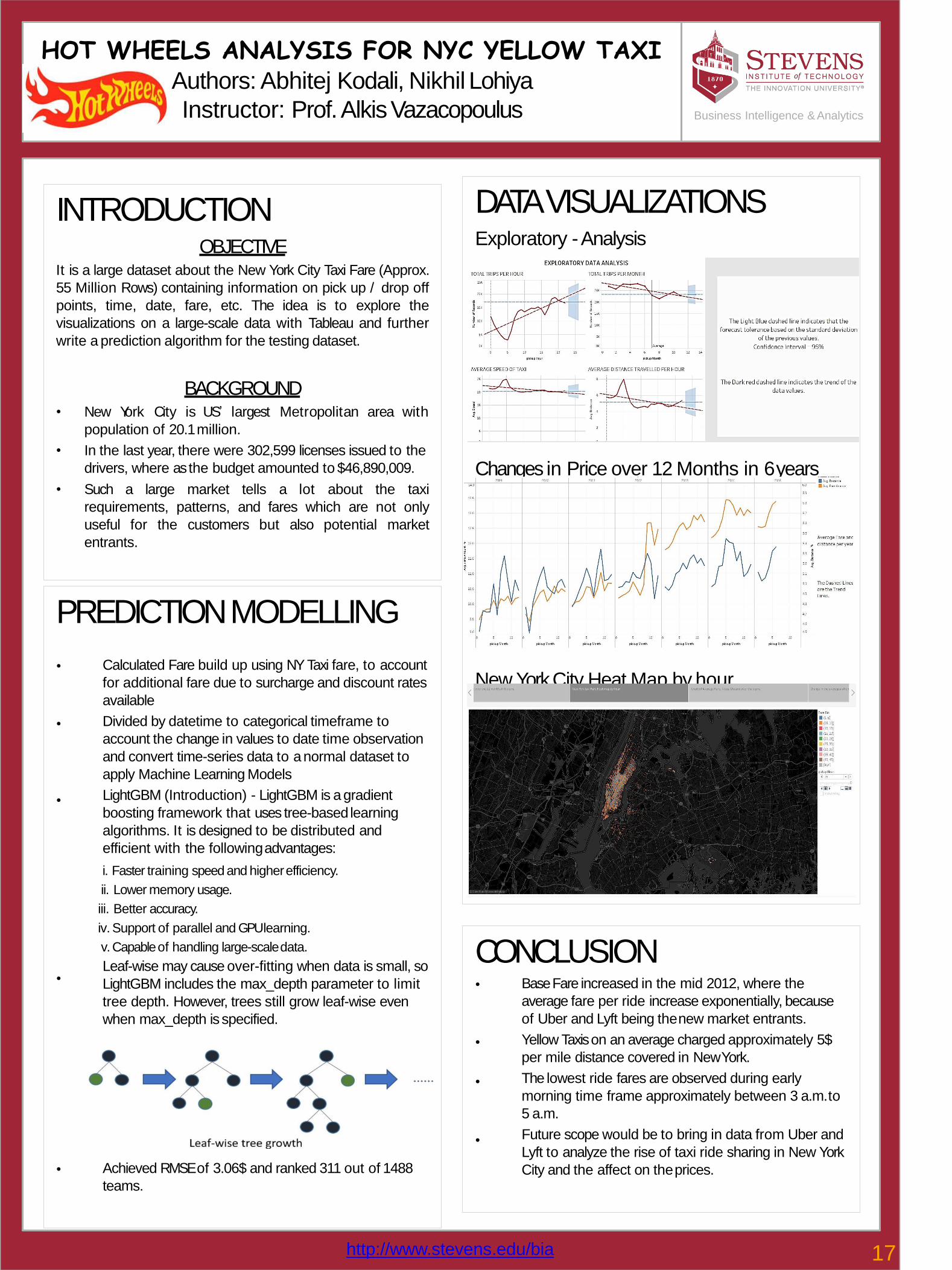
DATAVISUALIZATIONSExploratory -Analysis
Changes in Price over 12 Months in 6years
New York City Heat Map by hour
INTRODUCTIONOBJECTIVE
It is a large dataset about the New York City Taxi Fare (Approx.
55 Million Rows) containing information on pick up / drop off
points, time, date, fare, etc. The idea is to explore the
visualizations on a large-scale data with Tableau and further
write a prediction algorithm for the testing dataset.
BACKGROUND• New York City is US’ largest Metropolitan area with
population of 20.1million.
• In the last year, there were 302,599 licenses issued to the
drivers, where as the budget amounted to $46,890,009.
• Such a large market tells a lot about the taxi
requirements, patterns, and fares which are not only
useful for the customers but also potential market
entrants.
PREDICTIONMODELLING
•
•
•
•
Calculated Fare build up using NY Taxi fare, to account
for additional fare due to surcharge and discount rates
available
Divided by datetime to categorical timeframe to
account the change in values to date time observation
and convert time-series data to a normal dataset to
apply Machine Learning Models
LightGBM (Introduction) - LightGBM is a gradient
boosting framework that uses tree-based learning
algorithms. It is designed to be distributed and
efficient with the followingadvantages:
i. Faster training speed and higherefficiency.
ii. Lower memory usage.
iii. Better accuracy.
iv. Support of parallel and GPUlearning.
v. Capable of handling large-scaledata.
Leaf-wise may cause over-fitting when data is small, so
LightGBM includes the max_depth parameter to limit
tree depth. However, trees still grow leaf-wise even
when max_depth isspecified.
• Achieved RMSE of 3.06$ and ranked 311 out of 1488
teams.
CONCLUSION•
•
•
•
Base Fare increased in the mid 2012, where the
average fare per ride increase exponentially, because
of Uber and Lyft being thenew market entrants.
Yellow Taxis on an average charged approximately 5$
per mile distance covered in NewYork.
The lowest ride fares are observed during early
morning time frame approximately between 3 a.m.to
5 a.m.
Future scope would be to bring in data from Uber and
Lyft to analyze the rise of taxi ride sharing in New York
City and the affect on theprices.
Business Intelligence & Analytics
http://www.stevens.edu/bia 17
Customer Revenue Prediction for Google Store
ProductsAuthors: Nikhil Lohiya, Abhitej Kodali
Instructor: Prof. AlkisVazacopoulos
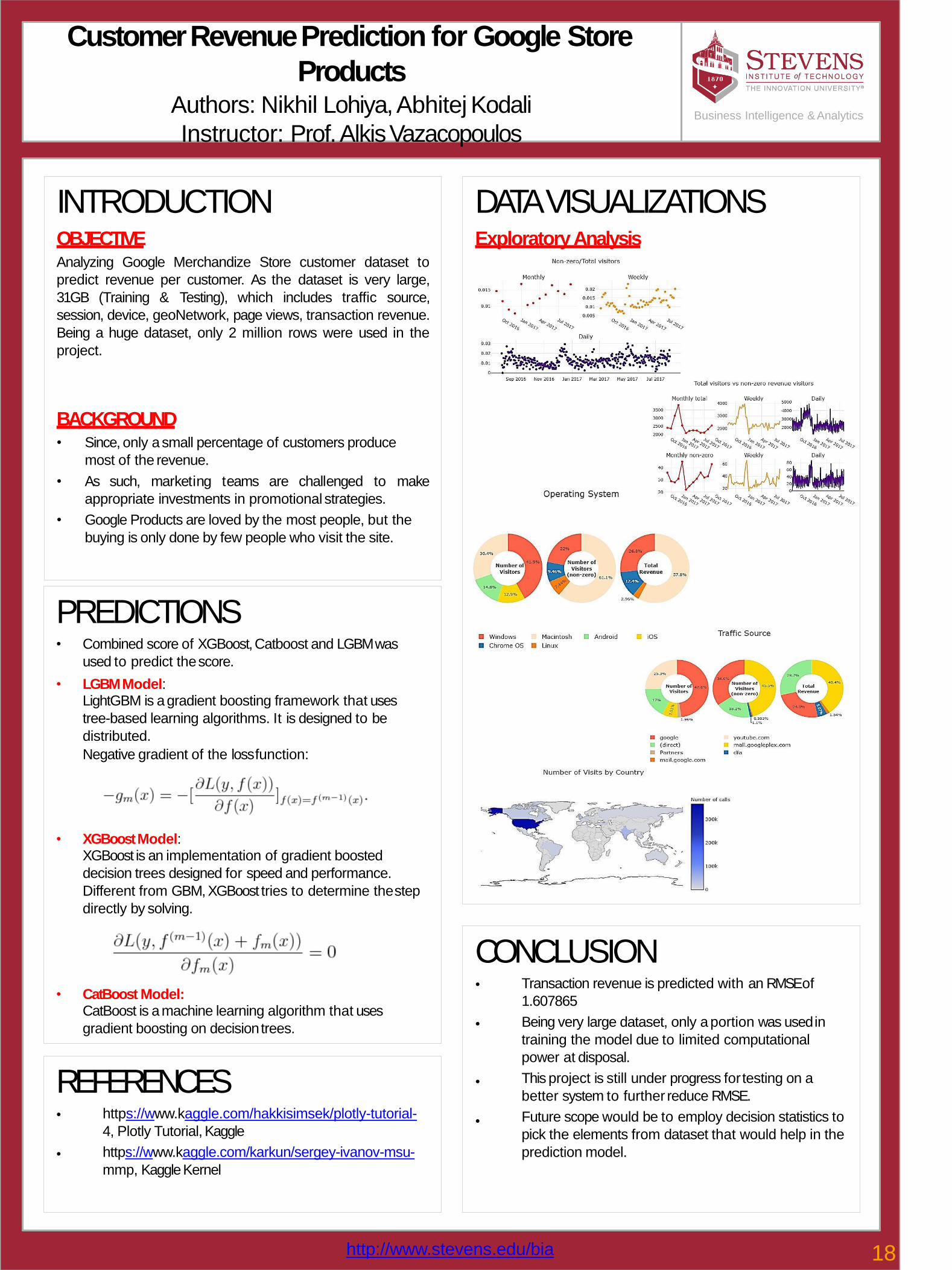
DATAVISUALIZATIONSExploratoryAnalysis
INTRODUCTIONOBJECTIVEAnalyzing Google Merchandize Store customer dataset to
predict revenue per customer. As the dataset is very large,
31GB (Training & Testing), which includes traffic source,
session, device, geoNetwork, page views, transaction revenue.
Being a huge dataset, only 2 million rows were used in the
project.
BACKGROUND• Since, only a small percentage of customers produce
most of the revenue.
• As such, marketing teams are challenged to make
appropriate investments in promotional strategies.
• Google Products are loved by the most people, but the
buying is only done by few people who visit the site.
PREDICTIONS• Combined score of XGBoost, Catboost and LGBM was
used to predict thescore.
• LGBMModel:LightGBM is a gradient boosting framework that uses
tree-based learning algorithms. It is designed to be
distributed.
Negative gradient of the lossfunction:
• XGBoostModel:XGBoost is an implementation of gradient boosted
decision trees designed for speed and performance.
Different from GBM, XGBoost tries to determine thestep
directly by solving.
• CatBoost Model:CatBoost is a machine learning algorithm that uses
gradient boosting on decisiontrees.
CONCLUSION•
•
•
•
Transaction revenue is predicted with an RMSEof
1.607865
Being very large dataset, only a portion was usedin
training the model due to limited computational
power at disposal.
This project is still under progress fortesting on a
better system to further reduce RMSE.
Future scope would be to employ decision statistics to
pick the elements from dataset that would help in the
prediction model.
Business Intelligence & Analytics
REFERENCES•
•
https://www.kaggle.com/hakkisimsek/plotly-tutorial-
4, Plotly Tutorial, Kaggle
https://www.kaggle.com/karkun/sergey-ivanov-msu-
mmp, KaggleKernel
http://www.stevens.edu/bia 18
Clustering Large Cap Stocks During Different Phases of the
EconomicCycleStudents: Nikhil Lohiya, Raj Mehta
Instructor: Amir H. Gandomi
Results
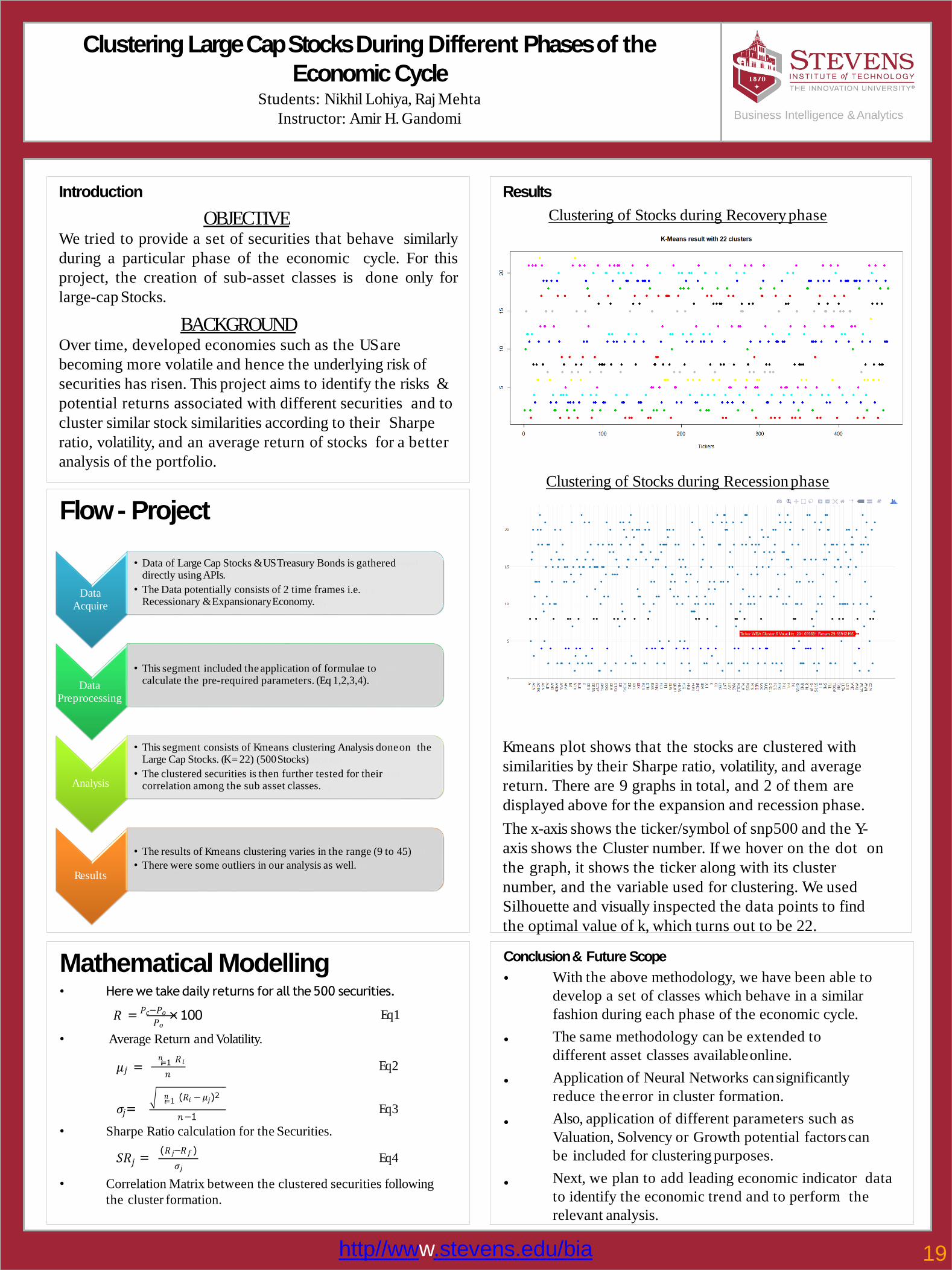
Clustering of Stocks during Recoveryphase
Clustering of Stocks during Recession phase
K means plot shows that the stocks are clustered with
similarities by their Sharpe ratio, volatility, and average
return. There are 9 graphs in total, and 2 of them are
displayed above for the expansion and recession phase.
The x-axis shows the ticker/symbol of snp500 and the Y-
axis shows the Cluster number. If we hover on the dot on
the graph, it shows the ticker along with its cluster
number, and the variable used for clustering. We used
Silhouette and visually inspected the data points to find
the optimal value of k, which turns out to be 22.
Introduction
OBJECTIVEWe tried to provide a set of securities that behave similarly
during a particular phase of the economic cycle. For this
project, the creation of sub-asset classes is done only for
large-cap Stocks.
BACKGROUNDOver time, developed economies such as the US are
becoming more volatile and hence the underlying risk of
securities has risen. This project aims to identify the risks &
potential returns associated with different securities and to
cluster similar stock similarities according to their Sharpe
ratio, volatility, and an average return of stocks for a better
analysis of the portfolio.
Business Intelligence & Analytics
http//www.stevens.edu/bia
Data
Acquire
• Data of Large Cap Stocks & US Treasury Bonds is gathered directly using APIs.
• The Data potentially consists of 2 time frames i.e. Recessionary & ExpansionaryEconomy.
Data
Preprocessing
• This segment included the application of formulae to calculate the pre-required parameters. (Eq 1,2,3,4).
Analysis
• This segment consists of K means clustering Analysis doneon the Large Cap Stocks. (K = 22) (500Stocks)
• The clustered securities is then further tested for their correlation among the sub asset classes.
Results
• The results of Kmeans clustering varies in the range (9 to 45)
• There were some outliers in our analysis as well.
Flow - Project
Conclusion & Future Scope
•
•
•
•
•
With the above methodology, we have been able to
develop a set of classes which behave in a similar
fashion during each phase of the economic cycle.
The same methodology can be extended to
different asset classes availableonline.
Application of Neural Networks cansignificantly
reduce the error in cluster formation.
Also, application of different parameters such as
Valuation, Solvency or Growth potential factorscan
be included for clustering purposes.
Next, we plan to add leading economic indicator data
to identify the economic trend and to perform the
relevant analysis.
Mathematical Modelling• Here we take daily returns for all the 500 securities.
𝑅 = 𝑃𝑐−𝑃𝑜×100
•
𝑃𝑜
Average Return and Volatility.
𝑗
Eq1
𝜇 =𝑅 𝑖𝑛
𝑖=1
𝑛Eq2
𝜎𝑗=(𝑅𝑖 −𝜇𝑗)2𝑛
𝑖=1
𝑛−1Eq3
• Sharpe Ratio calculation for the Securities.
𝑗𝑆𝑅 =(𝑅 𝑗−𝑅𝑓)
𝜎𝑗Eq4
• Correlation Matrix between the clustered securities following
the cluster formation.
19
FIN-FINICKY : Financial Analyst’s Toolkit
Author: NikhilLohiya
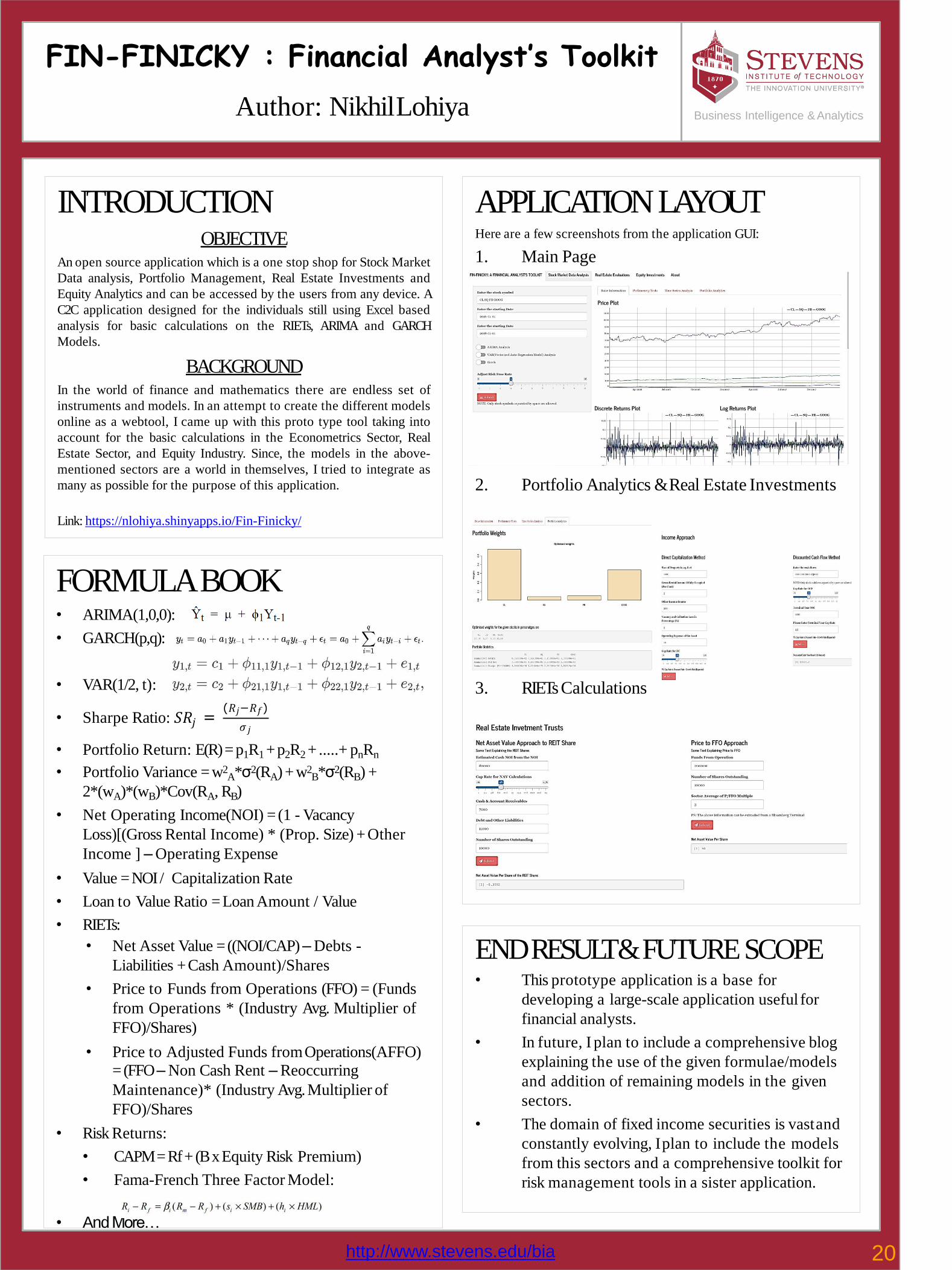
APPLICATIONLAYOUTHere are a few screenshots from the application GUI:
1. Main Page
2. Portfolio Analytics & Real Estate Investments
3. RIETsCalculations
INTRODUCTIONOBJECTIVE
An open source application which is a one stop shop for Stock Market
Data analysis, Portfolio Management, Real Estate Investments and
Equity Analytics and can be accessed by the users from any device. A
C2C application designed for the individuals still using Excel based
analysis for basic calculations on the RIETs, ARIMA and GARCH
Models.
BACKGROUNDIn the world of finance and mathematics there are endless set of
instruments and models. In an attempt to create the different models
online as a webtool, I came up with this proto type tool taking into
account for the basic calculations in the Econometrics Sector, Real
Estate Sector, and Equity Industry. Since, the models in the above-
mentioned sectors are a world in themselves, I tried to integrate as
many as possible for the purpose of this application.
Link: https://nlohiya.shinyapps.io/Fin-Finicky/
FORMULABOOK• ARIMA(1,0,0):
• GARCH(p,q):
𝑗(𝑅𝑗−𝑅𝑓)
𝜎 𝑗
• VAR(1/2, t):
• Sharpe Ratio: 𝑆𝑅 =
• Portfolio Return: E(R) = p1R1 + p2R2 + .....+ pnRn
• Portfolio Variance = w2A*σ2(RA) + w2
B*σ2(RB) +
2*(wA)*(wB)*Cov(RA, RB)
• Net Operating Income(NOI) = (1 - Vacancy
Loss)[(Gross Rental Income) * (Prop. Size) + Other
Income ] – Operating Expense
• Value = NOI / Capitalization Rate
• Loan to Value Ratio = Loan Amount / Value
• RIETs:
• Net Asset Value = ((NOI/CAP) – Debts -
Liabilities + Cash Amount)/Shares
• Price to Funds from Operations (FFO) = (Funds
from Operations * (Industry Avg. Multiplier of
FFO)/Shares)
• Price to Adjusted Funds fromOperations(AFFO)
= (FFO – Non Cash Rent – Reoccurring
Maintenance)* (Industry Avg. Multiplier of
FFO)/Shares
• Risk Returns:
• CAPM = Rf + (B x Equity Risk Premium)
• Fama-French Three Factor Model:
• And More…
END RESULT & FUTURESCOPE• This prototype application is a base for
developing a large-scale application useful for
financial analysts.
• In future, I plan to include a comprehensive blog
explaining the use of the given formulae/models
and addition of remaining models in the given
sectors.
• The domain of fixed income securities is vastand
constantly evolving, I plan to include the models
from this sectors and a comprehensive toolkit for
risk management tools in a sister application.
Business Intelligence & Analytics
20http://www.stevens.edu/bia
Group Emailing using Robotic Process AutomationAuthors: Pallavi Naidu, Abhitej Kodali
Instructor: Prof. Edward Stohr Business Intelligence &
Analytics
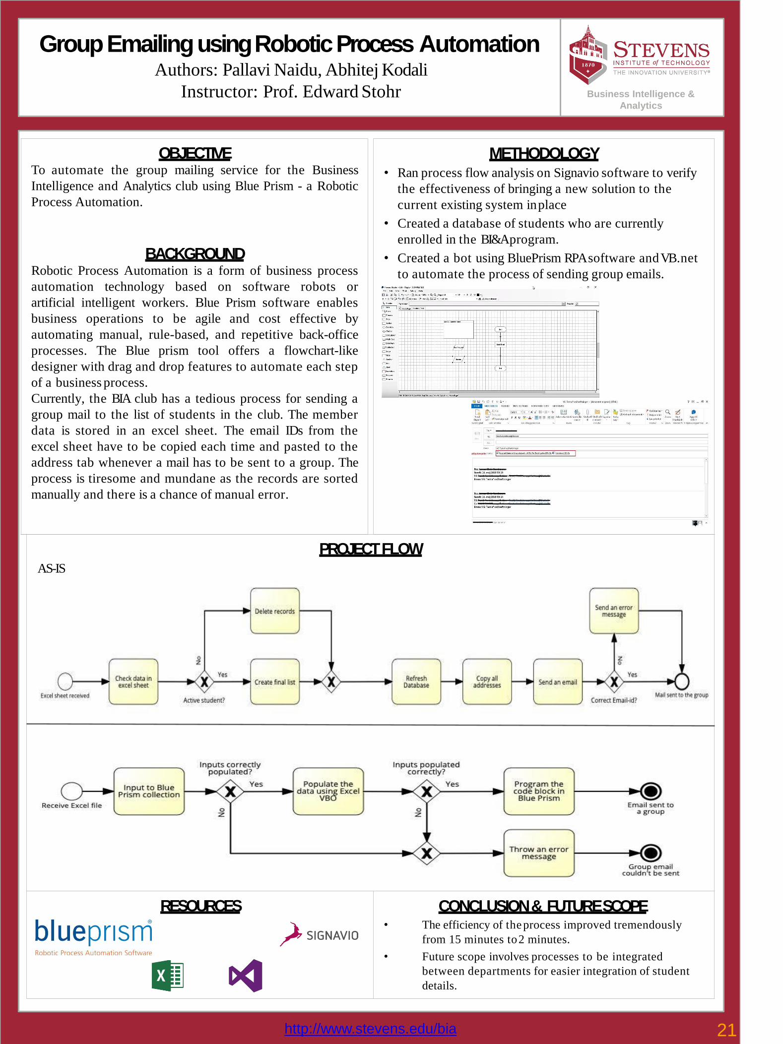
OBJECTIVETo automate the group mailing service for the Business
Intelligence and Analytics club using Blue Prism - a Robotic
Process Automation.
BACKGROUNDRobotic Process Automation is a form of business process
automation technology based on software robots or
artificial intelligent workers. Blue Prism software enables
business operations to be agile and cost effective by
automating manual, rule-based, and repetitive back-office
processes. The Blue prism tool offers a flowchart-like
designer with drag and drop features to automate each step
of a business process.
Currently, the BIA club has a tedious process for sending a
group mail to the list of students in the club. The member
data is stored in an excel sheet. The email IDs from the
excel sheet have to be copied each time and pasted to the
address tab whenever a mail has to be sent to a group. The
process is tiresome and mundane as the records are sorted
manually and there is a chance of manual error.
METHODOLOGY• Ran process flow analysis on Signavio software to verify
the effectiveness of bringing a new solution to the
current existing system inplace
• Created a database of students who are currently
enrolled in the BI&Aprogram.
• Created a bot using BluePrism RPA software andVB .net
to automate the process of sending group emails.
PROJECTFLOWAS-IS
SHOULD-BE
RESOURCES CONCLUSION & FUTURESCOPE• The efficiency of the process improved tremendously
from 15 minutes to2 minutes.
• Future scope involves processes to be integrated
between departments for easier integration of student
details.
21http://www.stevens.edu/bia

Cognitive Application to Determine Adverse Side Effects of
VaccinesAuthors: Pallavi Naidu, Kathy Chowaniec, KrishanuAgrawal
Instructor: Dr. ChrisAsakiewicz Business Intelligence &
Analytics
OBJECTIVETo develop a cognitive chat bot application that would
enable the public to discover the potential symptoms of a
particular vaccine based on their demographics using past
reported events from the VAERS Dataset. The vaccine bot
would be featured on a medical website to attract potential
users, but could be expanded to doctors and more
experienced medical professionals.
BACKGROUNDThe Centers for Disease Control and Prevention (CDC) and
the U.S. Food and Drug Administration (FDA) maintain a
database of adverse reactions to vaccines, called the
Vaccine Adverse Event Reporting System (VAERS).
According to the CDC, over 30,000 VAERS reports are filed
each year. By using this data, our chat bot would help users
know the symptoms of a reaction to a vaccine and the
number of days after which it would manifest. This would
help users to be aware of and be prepared for any adverse
events in the future.
DISCOVERYARCHITECTURE
Below is thestandard architecture for Watson Discovery:
To extract the symptom data, we used the Discovery
Language Query concept by building queries and
integrating them with ourapplication.
Discovery Language Query
We applied the Natural Language Query feature of Watson
Discovery, which gives results closest to the input when no
exact match is found from the Discovery language query.
Natural LanguageQuery
PROJECTFLOW
VAERS dataset of 2000 records
Cleaned and converted the files to JSON
Data format to upload to Watson DiscoveryProcessing
Queries using Watson Discovery Language
Analysisand Natural Language Query features
API to give symptoms by connecting
API Watson Assistant & Discovery applications
Vaccine Side Effects Chatbot which asks user demographics and gives results from
Results API accordingly
RESOURCES
• IBM Watson Assistant & Discoveryservices
• API using IBM CloudFunctions
• Languages: Python &JavaScript
• Bluemix/IBM Cloud deployment
FUTURESCOPE• Can be expanded to include pharmaceutical drug
symptoms from FEARSdataset
• Allow doctors and pharmacists to use chat bot in advising
and helping diagnose symptoms in patients
• Expand vaccine dataset for more accurate results
22http://www.stevens.edu/bia
Predict Potential Customers by Analyzing Bank’s
Telemarketing DataAuthors: Shreyas Menon, Pallavi Naidu
Instructor: Prof. DavidBelangerBusiness Intelligence &
Analytics
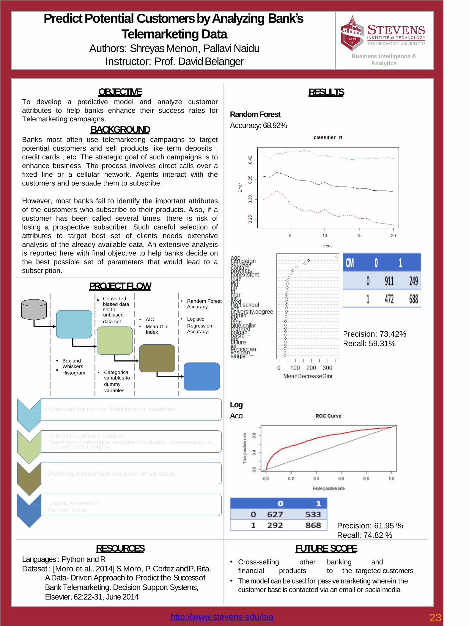
OBJECTIVETo develop a predictive model and analyze customer
attributes to help banks enhance their success rates for
Telemarketing campaigns.
BACKGROUNDBanks most often use telemarketing campaigns to target
potential customers and sell products like term deposits ,
credit cards , etc. The strategic goal of such campaigns is to
enhance business. The process involves direct calls over a
fixed line or a cellular network. Agents interact with the
customers and persuade them to subscribe.
However, most banks fail to identify the important attributes
of the customers who subscribe to their products. Also, if a
customer has been called several times, there is risk of
losing a prospective subscriber. Such careful selection of
attributes to target best set of clients needs extensive
analysis of the already available data. An extensive analysis
is reported here with final objective to help banks decide on
the best possible set of parameters that would lead to a
subscription.
RESULTS
RandomForest
Accuracy: 68.92%
Precision: 73.42%
Recall: 59.31%
LogisticRegression
Accuracy: 64.43%
Precision: 61.95 %
Recall: 74.82 %
PROJECTFLOW
• Converted• Random Forest
biased dataAccuracy:
Dataset set tounbiased
Data data set • AIC • Logistic
Exploration • Mean Gini Regression
Index Accuracy:
Data
Preprocessing
Variable• Box and Selection
Whiskers• Histogram • Categorical Classification
variables to and
dummy Prediction
variables
• Checked the normal distribution of variablesData
Exploration
• Deleted insignificant variables• Transformed categorical variables into dummy representation to
Data preserve useful insightsPreprocessing
• Performed dimension reduction on variablesVariableSelection
• Logistic RegressionClassification • Random forestand Prediction
RESOURCESLanguages : Python andR
Dataset : [Moro et al., 2014] S. Moro, P. Cortez andP. Rita.A Data- Driven Approach to Predict the Successof
Bank Telemarketing. Decision Support Systems,
Elsevier, 62:22-31, June2014
FUTURESCOPE
• Cross-selling other banking and
financial products to the targeted customers
• The model can be used for passive marketing wherein the
customer base is contacted via an email or socialmedia
23http://www.stevens.edu/bia
Quora - Answer Recommendation Using
Deep Learning ModelsAuthors: Tsen-Hung Wu, Cheng Yu, Shreyas Menon
Instructor: Rong Liu
Results and Evaluations• Selected the best similarity score threshold
to achieve the optimal model performance on test data (CNN)
BackgroundQuora is a question-and-answer website where askers can post
questions or find answers. Around 38 millions of questions have been
asked on Quora. To be more specific, we focused on the topic of Bitcoin
discussed on Quora because it becoming a popular topic recently.
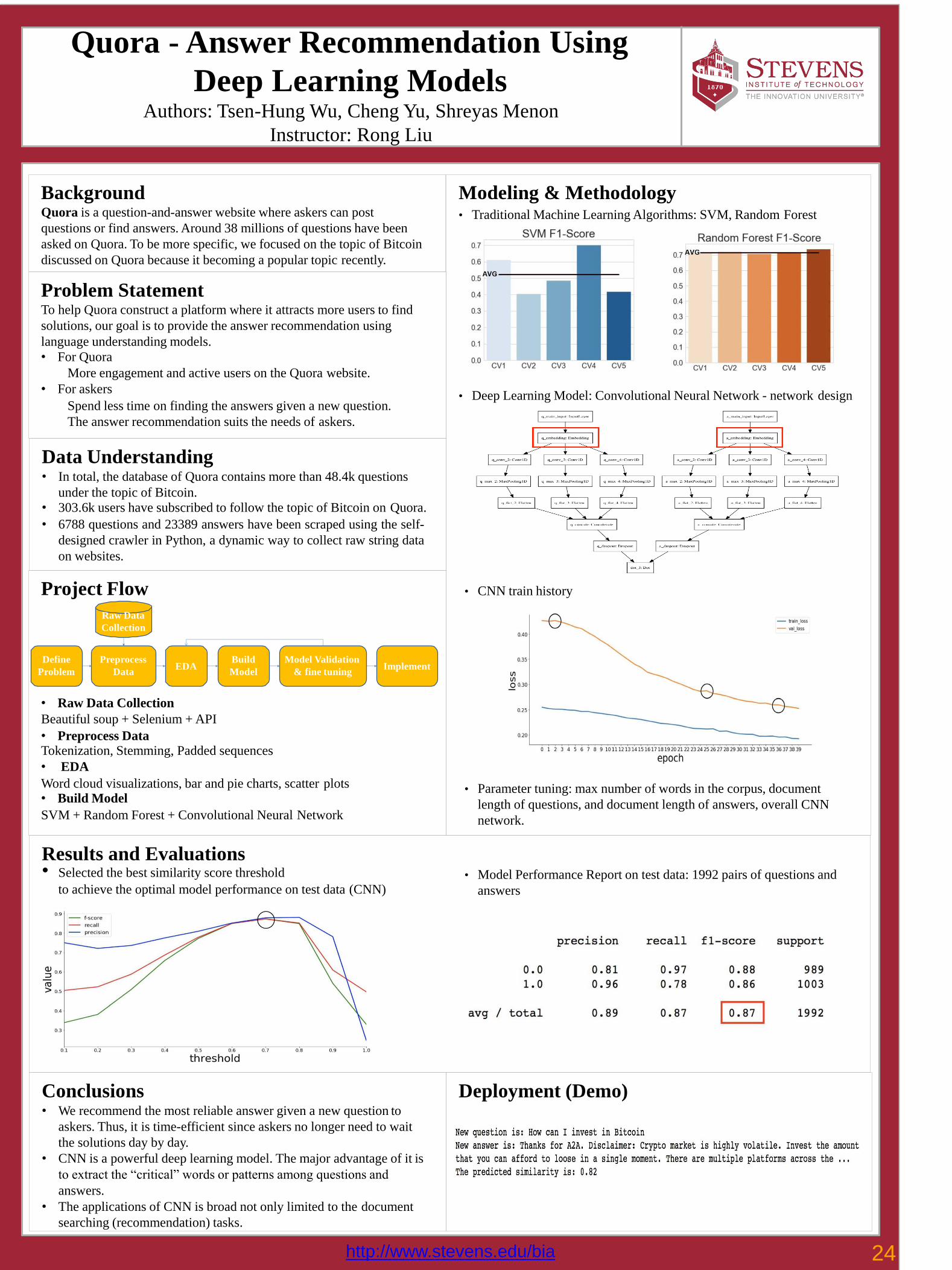
Modeling & Methodology• Traditional Machine Learning Algorithms: SVM, Random Forest
• Deep Learning Model: Convolutional Neural Network - network design
• CNN train history
• Parameter tuning: max number of words in the corpus, document
length of questions, and document length of answers, overall CNN
network.
• Model Performance Report on test data: 1992 pairs of questions and
answers
Problem StatementTo help Quora construct a platform where it attracts more users to find
solutions, our goal is to provide the answer recommendation using
language understanding models.
• For Quora
More engagement and active users on the Quora website.
• For askers
Spend less time on finding the answers given a new question.
The answer recommendation suits the needs of askers.
Data Understanding• In total, the database of Quora contains more than 48.4k questions
under the topic of Bitcoin.
• 303.6k users have subscribed to follow the topic of Bitcoin on Quora.
• 6788 questions and 23389 answers have been scraped using the self-
designed crawler in Python, a dynamic way to collect raw string data
on websites.
• Raw Data Collection
Beautiful soup + Selenium + API
• Preprocess DataTokenization, Stemming, Padded sequences
• EDA
Word cloud visualizations, bar and pie charts, scatter plots• Build Model
SVM + Random Forest + Convolutional Neural Network
Conclusions• We recommend the most reliable answer given a new question to
askers. Thus, it is time-efficient since askers no longer need to wait
the solutions day by day.
• CNN is a powerful deep learning model. The major advantage of it is
to extract the “critical” words or patterns among questions and
answers.
• The applications of CNN is broad not only limited to the document
searching (recommendation) tasks.
Deployment (Demo)
Define
Problem
Preprocess
Data
Project Flow
Raw Data
Collection
EDABuild
Model
Model Validation
& fine tuningImplement
24http://www.stevens.edu/bia
LendingClub – How to Forecast the Loan Status of Loan Applications?
Use Machine Learning Algorithms to Predict the Probability of Defaulting
Authors: Tsen-Hung Wu, Shreyas Menon
Instructor: Rong Liu
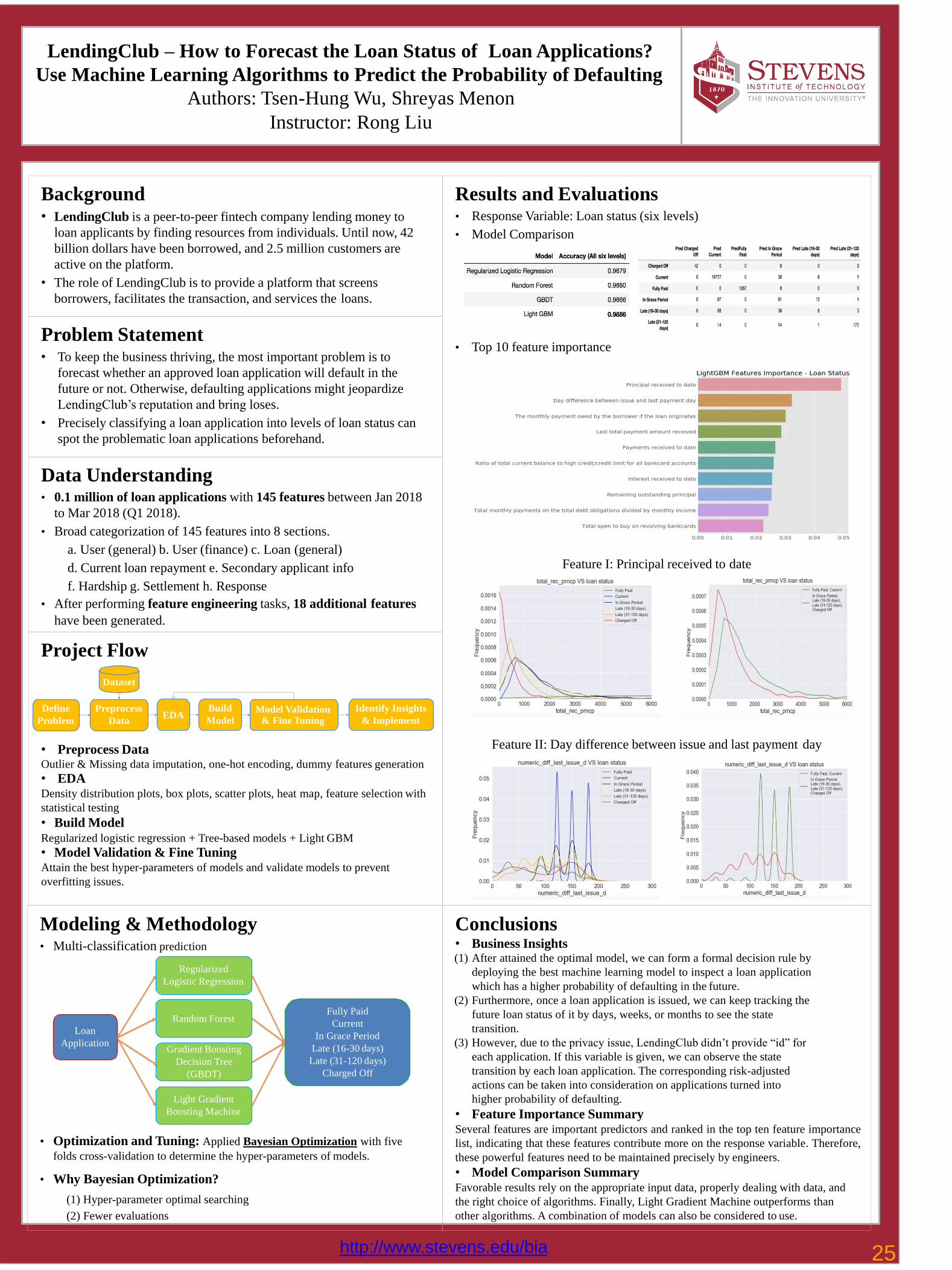
• Response Variable: Loan status (six levels)
• Model Comparison
• Top 10 feature importance
Feature I: Principal received to date
Feature II: Day difference between issue and last payment day
Background Results and Evaluations• LendingClub is a peer-to-peer fintech company lending money to
loan applicants by finding resources from individuals. Until now, 42
billion dollars have been borrowed, and 2.5 million customers are
active on the platform.
• The role of LendingClub is to provide a platform that screens
borrowers, facilitates the transaction, and services the loans.
• Optimization and Tuning: Applied Bayesian Optimization with five
folds cross-validation to determine the hyper-parameters of models.
• Why Bayesian Optimization?
(1) Hyper-parameter optimal searching
(2) Fewer evaluations
Problem Statement• To keep the business thriving, the most important problem is to
forecast whether an approved loan application will default in the
future or not. Otherwise, defaulting applications might jeopardize
LendingClub’s reputation and bring loses.
• Precisely classifying a loan application into levels of loan status can
spot the problematic loan applications beforehand.
Data Understanding• 0.1 million of loan applications with 145 features between Jan 2018
to Mar 2018 (Q1 2018).
• Broad categorization of 145 features into 8 sections.
a. User (general) b. User (finance) c. Loan (general)
d. Current loan repayment e. Secondary applicant info
f. Hardship g. Settlement h. Response
• After performing feature engineering tasks, 18 additional features
have been generated.
• Preprocess DataOutlier & Missing data imputation, one-hot encoding, dummy features generation
• EDADensity distribution plots, box plots, scatter plots, heat map, feature selection with
statistical testing
• Build Model
Regularized logistic regression + Tree-based models + Light GBM
• Model Validation & Fine TuningAttain the best hyper-parameters of models and validate models to prevent
overfitting issues.
Conclusions• Business Insights(1) After attained the optimal model, we can form a formal decision rule by
deploying the best machine learning model to inspect a loan application
which has a higher probability of defaulting in the future.
(2) Furthermore, once a loan application is issued, we can keep tracking the
future loan status of it by days, weeks, or months to see the state
transition.
(3) However, due to the privacy issue, LendingClub didn’t provide “id” for
each application. If this variable is given, we can observe the state
transition by each loan application. The corresponding risk-adjusted
actions can be taken into consideration on applications turned into
higher probability of defaulting.
• Feature Importance SummarySeveral features are important predictors and ranked in the top ten feature importance
list, indicating that these features contribute more on the response variable. Therefore,
these powerful features need to be maintained precisely by engineers.
• Model Comparison SummaryFavorable results rely on the appropriate input data, properly dealing with data, and
the right choice of algorithms. Finally, Light Gradient Machine outperforms than
other algorithms. A combination of models can also be considered to use.
Project Flow
Dataset
Define
Problem
Preprocess
DataEDA
Build
Model
Model Validation
& Fine Tuning
Identify Insights
& Implement
Modeling & Methodology• Multi-classification prediction
Regularized
Logistic Regression
Random Forest
Gradient Boosting
Decision Tree
(GBDT)
Light Gradient
Boosting Machine
Loan
Application
Fully Paid
Current
In Grace Period
Late (16-30 days)
Late (31-120 days)
Charged Off
25http://www.stevens.edu/bia

Visualization of Chicago CrimeAuthors: Xuanyan Li, Zihan Chen
Instructor: Prof. Alkiviadis Vazacopoulos Business Intelligence & Analytics
IntroductionUsing Tableau and Python, we shows the distribution of
each kind of crimes in Chicago city on the map. This
poster also tries to explore the relationship between
prime crime type and time period (Hour, Month &
Date), geographic information, criminal citizenship and
FBI code.
Data Source:
Crimes - 2001 to Present, Chicago Data Portal Website
https://data.cityofchicago.org/
Hours – Location Relationship
26http://www.stevens.edu/bia
These graphs show the different Chicago crime distribution in
each hour. We select 5:00 am and 5:00 pm to display the result.
Domestic – Prime Type Relationship
Following graphs show how criminal citizenship relate with
crime prime type, as well as the relationship with each location.
Arrest – Type & Location Relationship
Here are the results of whether a criminal was been arrested in
different time period, crime type and location information.
Prime Type – Location & Month Relationship
These four pictures utilizing maps and bar graphs to show the
trend and distribution of each crime in different year, month
and location. We select Narcotics to demonstrate the results.
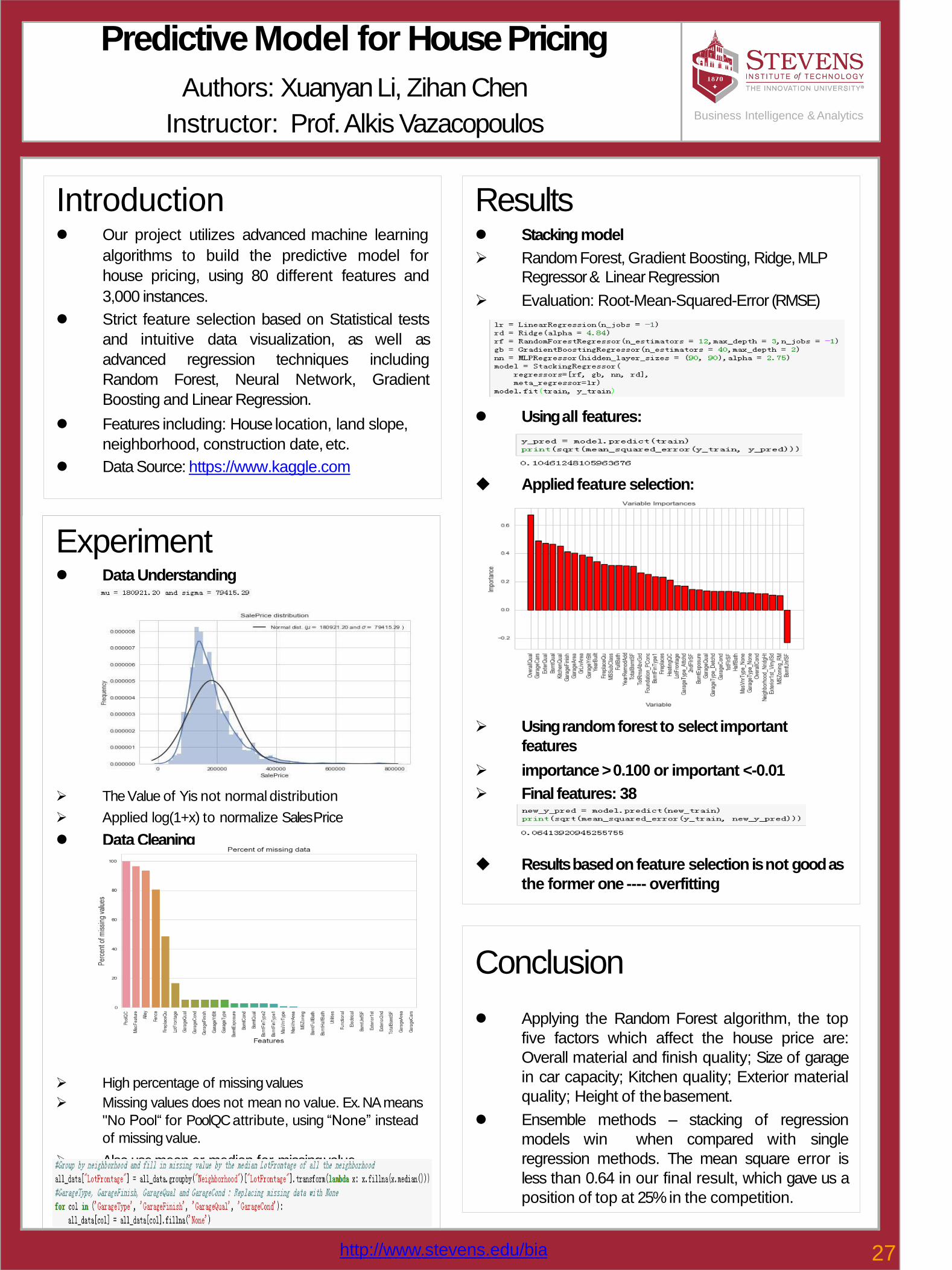
Business Intelligence & Analytics
Predictive Model for HousePricing
Authors: Xuanyan Li, Zihan Chen
Instructor: Prof. Alkis Vazacopoulos
Introduction Results⚫ Our project utilizes advanced machine learning ⚫ Stacking model
algorithms to build the predictive model for ➢ Random Forest, Gradient Boosting, Ridge, MLP house pricing, using 80 different features and Regressor & LinearRegression
3,000 instances. ➢ Evaluation: Root-Mean-Squared-Error (RMSE)⚫ Strict feature selection based on Statistical tests
and intuitive data visualization, as well as
advanced regression techniques including
Random Forest, Neural Network, Gradient
Boosting and Linear Regression.
⚫ Features including: House location, land slope, ⚫ Using all features:
neighborhood, construction date,etc.
⚫ Data Source: https://www.kaggle.com◆ Applied feature selection:
Experiment⚫ Data Understanding
➢ The Value of Y is not normal distribution
➢ Applied log(1+x) to normalize SalesPrice
⚫ Data Cleaning
➢ High percentage of missingvalues
➢ Missing values does not mean no value. Ex. NA means
"No Pool“ for PoolQC attribute, using “None” instead
of missing value.
➢ Also use mean or median for missingvalue
➢ Using random forest to select important
features
➢ importance > 0.100 or important <-0.01
➢ Final features: 38
◆ Results based on feature selection is not good as
the former one ---- overfitting
Conclusion
⚫ Applying the Random Forest algorithm, the top
five factors which affect the house price are:
Overall material and finish quality; Size of garage
in car capacity; Kitchen quality; Exterior material
quality; Height of thebasement.
⚫ Ensemble methods – stacking of regression
models win when compared with single
regression methods. The mean square error is
less than 0.64 in our final result, which gave us a
position of top at 25%in the competition.
27http://www.stevens.edu/bia

DOE for Amazon RecommendationEmailAuthors: Siyan Zhang, Xuanyan Li, Biyan Xie
Instructor: Prof. ChihoonLee
ProjectApproaches:
Future improvement:1.To improve responses: a) increase replications; b) use click-through rate as a
response;
2.To acquire better data: randomly select students from a school’s enrollment list;
3. To improve survey method: send emails to respondents simultaneously.
Business Intelligence & Analytics
Keywords& Programs:- JMP
- Fractional Factorial Design
BusinessQuestions:How can a company effectively attract people to visit thewebsite and
convert the browsers intobuyers?
Objectives:1.What are the important factors in Amazon recommendation emails
2.How to apply fractional factorial design to test best combination of
factor levels
ExperimentalDesign:1. Fractional factorial design with 6 factors and 2blocks:
2. 16 recommendation emails were created with 3 responses foreach
3. Target Audience: Students at Stevens Institute ofTechnology
Factors Lower Level (-) Higher Level (+)
1 Sender’s name Amazon.com Amazon.com
Recommendation
s
2 Subject Laptops... HP Flyer Red 15.6 Inch...
3 Ad’s content Popular product on
Amazon
(e.g. Amazon Echo)
Similar product with
recommended ones
(e.g. Samsung Odyssey 15.6)
4 Ad’s placement On the top of the
On the bottom of theemail
5 Provide rating and review
numbers
Yes No
6 Product list sortingby
price
Randomly From lowest to highest
Block Membership status 1: Non-prime 2: Prime
Results:
Significant Factors:
●Subject
●Rating and Review●Sender’s name*Subject
●Sender’s name*Sortby
price
(* denotes interactioneffect)
1. ParetoPlot:
significant
effects
(above line)
2. Normal Plot:
Regression Equation: Expected Response Under
Best Experiment Setting: Recommendation:
- Provide rating and
review numbers:Yes
- Product list sortingby
price: Random
- Sender’s name:Amazon.com
- Subject: Specificproducts
1. Examine the
distribution of data
2. Examine the
variance of each run
(experimental error)
28http://www.stevens.edu/bia
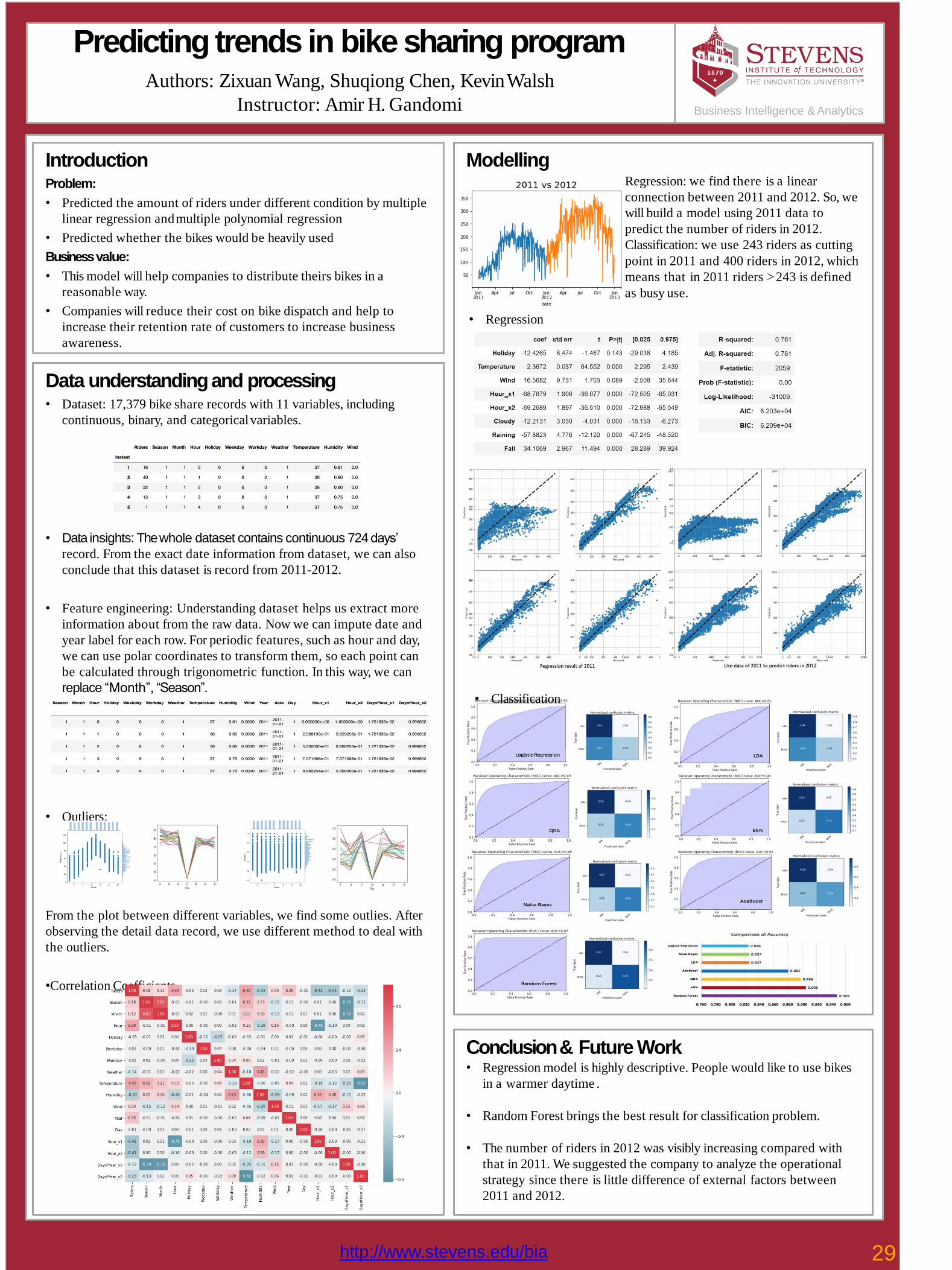
Predicting trends in bike sharing programAuthors: Zixuan Wang, Shuqiong Chen, KevinWalsh
Instructor: Amir H. Gandomi Business Intelligence & Analytics
IntroductionProblem:
• Predicted the amount of riders under different condition by multiple
linear regression andmultiple polynomial regression
• Predicted whether the bikes would be heavily used
Businessvalue:
• This model will help companies to distribute theirs bikes in a
reasonable way.
• Companies will reduce their cost on bike dispatch and help to
increase their retention rate of customers to increase business
awareness.
Data understanding and processing• Dataset: 17,379 bike share records with 11 variables, including
continuous, binary, and categoricalvariables.
• Data insights: The whole dataset contains continuous 724 days’
record. From the exact date information from dataset, we can also
conclude that this dataset is record from 2011-2012.
• Feature engineering: Understanding dataset helps us extract more
information about from the raw data. Now we can impute date and
year label for each row. For periodic features, such as hour and day,
we can use polar coordinates to transform them, so each point can
be calculated through trigonometric function. In this way, we can
replace “Month”, “Season”.
• Outliers:
From the plot between different variables, we find some outlies. After
observing the detail data record, we use different method to deal with
the outliers.
•Correlation Coefficients
Conclusion & Future Work• Regression model is highly descriptive. People would like to use bikes
in a warmer daytime .
• Random Forest brings the best result for classification problem.
• The number of riders in 2012 was visibly increasing compared with
that in 2011. We suggested the company to analyze the operational
strategy since there is little difference of external factors between
2011 and 2012.
ModellingRegression: we find there is a linear
connection between 2011 and 2012. So, we
will build a model using 2011 data to
predict the number of riders in 2012.
Classification: we use 243 riders as cutting
point in 2011 and 400 riders in 2012, which
means that in 2011 riders > 243 is defined
as busy use.
• Regression
• Classification
29http://www.stevens.edu/bia
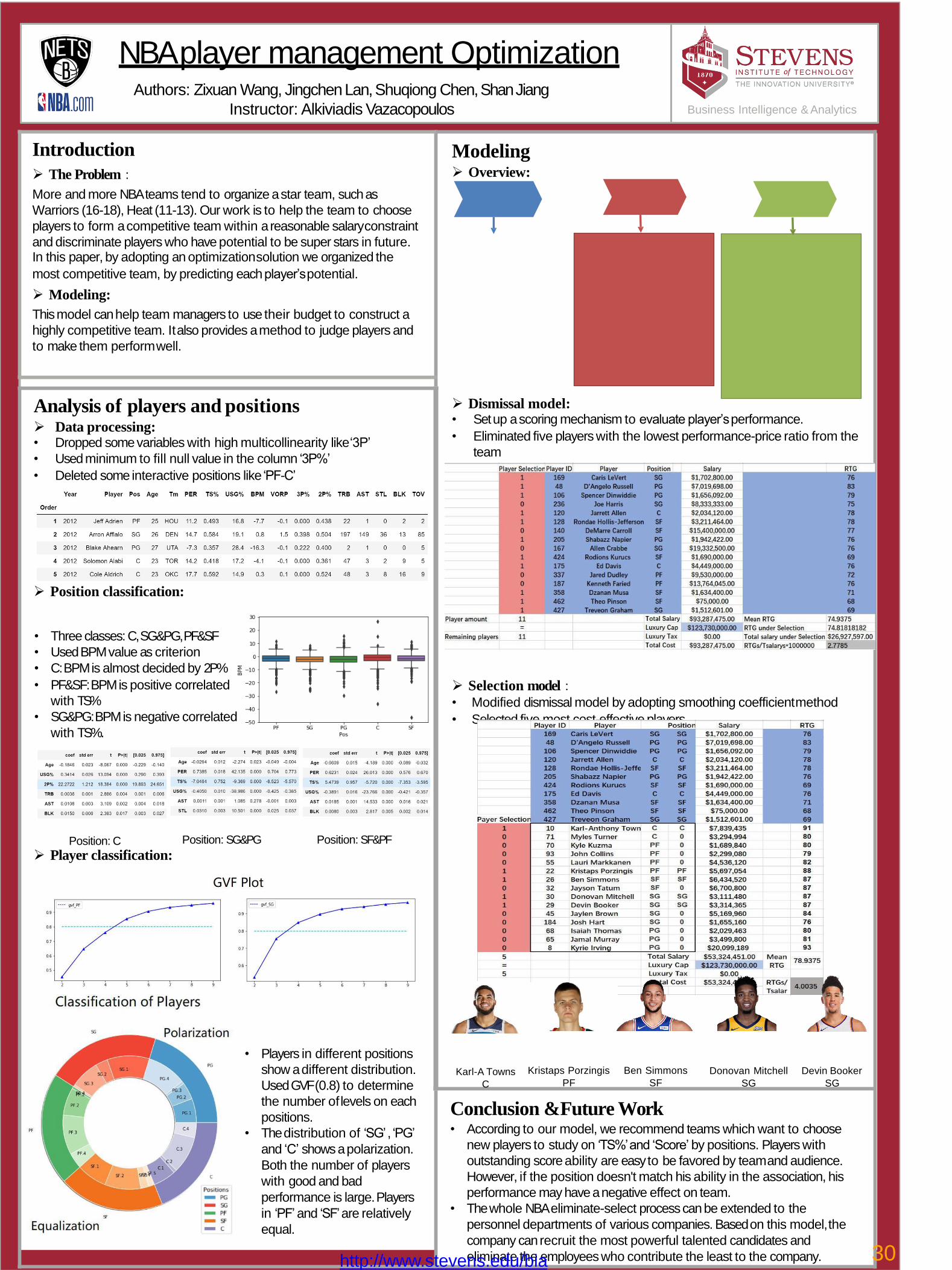
NBA player management OptimizationAuthors: Zixuan Wang, Jingchen Lan, Shuqiong Chen, Shan Jiang
Instructor: Alkiviadis Vazacopoulos Business Intelligence & Analytics
Introduction
➢ The Problem:
More and more NBA teams tend to organize a star team, such as
Warriors (16-18), Heat (11-13). Our work is to help the team to choose
players to form a competitive team within a reasonable salaryconstraint
and discriminate players who have potential to be super stars in future.In this paper, by adopting an optimizationsolution we organized the
most competitive team, by predicting each player’spotential.
➢ Modeling:
This model can help team managers to use their budget to construct a
highly competitive team. Italso provides a method to judge players and
to make them performwell.
Modeling➢ Overview:
Dismissal Candidate Selection
model pre-selection model
First, we set up a scoring Second, using the traditional Finally, considering the actual
mechanism to measure the "trial and error" method, and situation, most players in the
player's performance-price based on the existing scoring league are strong enough to
ratio according to the score mechanism, an adjusted replace other’s position.
of 2K19 combined with the parameter is established. We Therefore, in order to get the
salary given by the league, give the players measurement final model, we use the
according to the player's criteria under the constraint of smoothing coefficient method
performance-price ratio we different positions and select to modify the dismissalmodel.
eliminated five players with several strong candidates in Finally, five of the most cost-
the lowest performance- different positions from the effective players were selected
price ratio from the team pool of players in the league. from the candidates to fillthe
vacancies in the team position.
➢ Dismissal model:• Set up a scoring mechanism to evaluate player’sperformance.
• Eliminated five players with the lowest performance-price ratio from the
team
➢ Selection model:• Modified dismissal model by adopting smoothing coefficientmethod
• Selected five most cost-effective players
Karl-A Towns Kristaps Porzingis Ben Simmons Donovan Mitchell Devin Booker
C PF SF SG SG
Analysis of players and positions➢ Data processing:• Dropped some variables with high multicollinearity like‘3P’
• Usedminimum to fill null value in the column ‘3P%’
• Deleted some interactive positions like ‘PF-C’
➢ Position classification:
• Three classes: C, SG&PG,PF&SF
• Used BPM value as criterion
• C: BPM is almost decided by 2P%
• PF&SF: BPM is positive correlated
with TS%
• SG&PG: BPM is negative correlated
with TS%.
Position: C Position: SG&PG Position: SF&PF
➢ Player classification:
• Players in different positions
show a different distribution.
Used GVF (0.8) to determine
the number oflevels on each
positions.
• The distribution of ‘SG’ , ‘PG’
and ‘C’ shows a polarization.
Both the number of players
with good and bad
performance is large.Players
in ‘PF’ and ‘SF’ are relatively
equal.
Conclusion & Future Work• According to our model, we recommend teams which want to choose
new players to study on ‘TS%’ and ‘Score’ by positions. Players with
outstanding score ability are easy to be favored by teamand audience.
However, if the position doesn't match his ability in the association, his
performance may have a negative effect on team.
• The whole NBA eliminate-select process can be extended to the
personnel departments of various companies. Based on this model,the
company can recruit the most powerful talented candidates and
eliminate the employeeswho contribute the least to the company. 30http://www.stevens.edu/bia

Improvement of medical wire manufacturingAuthors: Zixuan Wang, Jingchen Lan
Instructor: Chihoon LeeBusiness Intelligence & Analytics
Conclusion
• We find the manufacturing of medical wires is a multi-factor
interactive process. Experiments of changing one factor at a
time may not maximize the YieldStrength
• For a medical wire manufacturer, we recommend using a
short bearing length and wide reduction angle with type 2
machine (even machine is not a significant factor).
SpoolIDBlo
2
ck
Mac
h 1
ine
Angl
e 0
Lengt
h
0
Diam
e
0
ter Order YS/UTS
0 1
93.3
26 1 1 0 0 1 2 92.5
9 1 0 1 0 1 3 92.9
35 1 1 1 0 0 4 93.5
11 1 0 0 1 1 5 93.2
36 1 1 0 1 0 6 92.4
5 1 0 1 1 0 7 93.7
29 1 1 1 1 1 8 92.9
New responsevariable
Avg(YS/UTS)
1/Avg(YS/UTS)
Log(YS/UTS)
Spool ID Machine Angle Length Diameter Mean
20 0 0 0 3 93.43
47 0 0 1 7 93.34
46 0 1 0 20 93.36
23 0 1 1 6 93.3
13 1 0 0 12 93.42
18 1 0 1 15 92.23
14 1 1 0 19 94.2641 1 1 1 4 94.04
Medical wire is a very inconspicuous device but plays a bigrole
during the surgery. The strength of the Medical wire is critical.
Problem:
• Design an experiment with four main factors to test the
effects of factors or interactions to the Yield Strength of the
medical wire.
• Find the combination that will yield the best quality of
medical wire.
Implications:
• This experiment will help manufacturers to select a more
suitable method to improve efficiency and quality on their
operation.
Fractional factorial design• Design of experiment:
24−1 fractional factorial with 4 factors, 3 blocks and5
replications.
We used 24 different spools at this level ofexperiment.
From figures above, we replaced the outliers by theaverage
value in their spoolthen:
R-square adj=44%
• Improvement:
Significant Factors:X2(Angle); X3(Length); X1(Machine)&X2(Angle);
X1(Machine)&X3(Length)With DV:Avg(YS/UTS)
R-square adj=56%
Full factorial design• Design of experiment:
23 Full FD with 3 factors and 3 replications. We used new set
of spools at this level to avoid bias.
Significant Factors:
B(Angle); A(Machine)&B(Angle); B(Angle)& C(Length)
R-square adj=87%
• Regression equation
𝒀 = 𝟎.𝟒𝟏 ∗𝑩 +𝟎.𝟑𝟓 ∗𝑨𝑩 + 𝟎.𝟏𝟔 ∗𝑩𝑪 + 𝟗𝟑.𝟒
• Effect graph:From the main effect and interaction plots wecan make a
conclusion that optimization of the process may be a
consequence of the combination ofmultifactor.
• Outliers:Conducted a regression analysis using the design table
directly.
R-Square adj=28%
Soit is necessary to explore the data and try to exclude
outliers.
• Correlation coefficient
After exploring themodel’s correlation, we
decide to use X1, X2
and X3 to design a full
factorial experiment in
the next step.
http://www.stevens.edu/bia 31
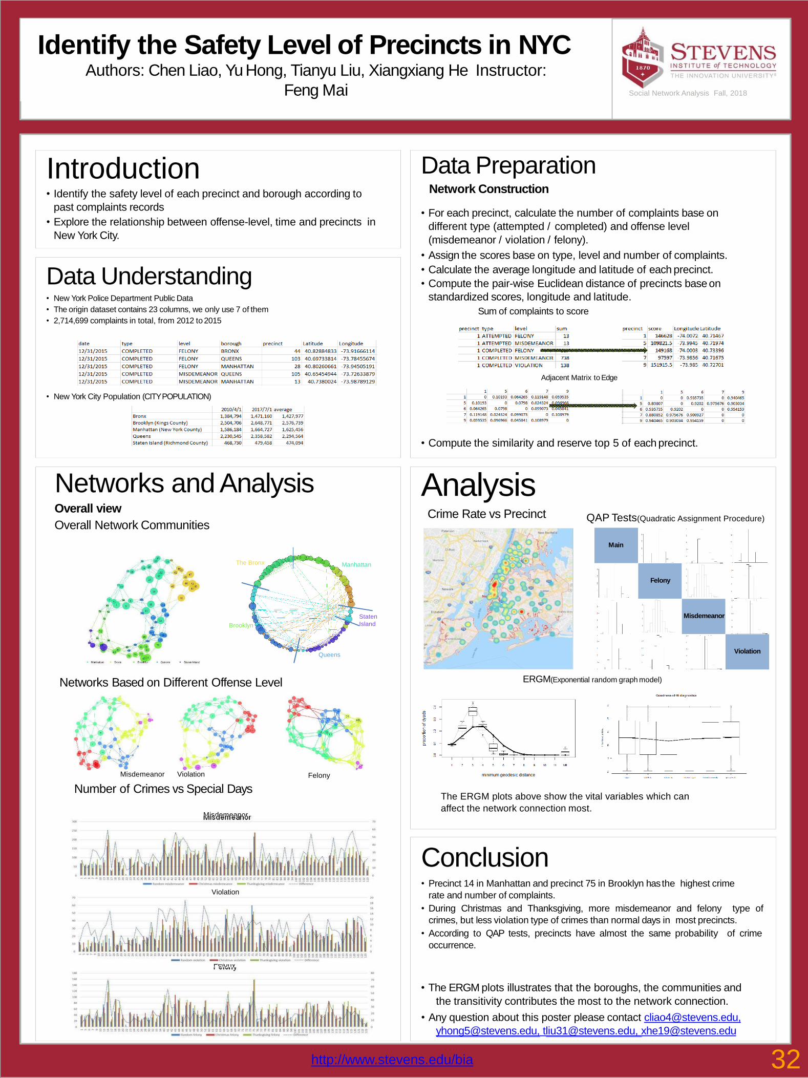
Identify the Safety Level of Precincts in NYCAuthors: Chen Liao, Yu Hong, Tianyu Liu, Xiangxiang He Instructor:
Feng Mai
Networks and AnalysisOverall view
Overall Network Communities
Networks Based on Different Offense Level
Introduction• Identify the safety level of each precinct and borough according to
past complaints records
• Explore the relationship between offense-level, time and precincts in
New York City.
Conclusion• Precinct 14 in Manhattan and precinct 75 in Brooklyn hasthe highest crime
rate and number of complaints.
• During Christmas and Thanksgiving, more misdemeanor and felony type of
crimes, but less violation type of crimes than normal days in most precincts.
• According to QAP tests, precincts have almost the same probability of crime
occurrence.
• The ERGM plots illustrates that the boroughs, the communities and
the transitivity contributes the most to the network connection.
• Any question about this poster please contact [email protected],
[email protected], [email protected], [email protected]
Social Network Analysis Fall, 2018
Data Understanding• New York Police Department Public Data
• The origin dataset contains 23 columns, we only use 7 of them
• 2,714,699 complaints in total, from 2012 to 2015
• New York City Population (CITYPOPULATION)
Data PreparationNetwork Construction
• For each precinct, calculate the number of complaints base on
different type (attempted / completed) and offense level
(misdemeanor / violation / felony).
• Assign the scores base on type, level and number of complaints.
• Calculate the average longitude and latitude of each precinct.
• Compute the pair-wise Euclidean distance of precincts base on
standardized scores, longitude and latitude.
Sum of complaints to score
Adjacent Matrix to Edge
• Compute the similarity and reserve top 5 of each precinct.
AnalysisCrime Rate vs Precinct QAP Tests(Quadratic Assignment Procedure)
ERGM(Exponential random graph model)
Misdemeanor Violation
Number of Crimes vs Special Days
Felony
Misdemeanor
Felony
ManhattanThe Bronx
Brooklyn
Queens
Staten
Island
Violation
Main
Felony
Misdemeanor
Violation
The ERGM plots above show the vital variables which can
affect the network connection most.
http://www.stevens.edu/bia 32
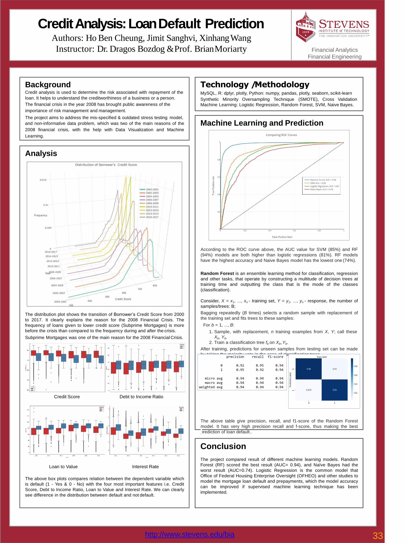
Credit Analysis: Loan Default PredictionAuthors: Ho Ben Cheung, Jimit Sanghvi, XinhangWang
Instructor: Dr. Dragos Bozdog & Prof. BrianMoriarty Financial Analytics
Financial Engineering
BackgroundCredit analysis is used to determine the risk associated with repayment of the
loan. It helps to understand the creditworthiness of a business or a person.
The financial crisis in the year 2008 has brought public awareness of the
importance of risk management and management.
The project aims to address the mis-specified & outdated stress testing model,
and non-informative data problem, which was two of the main reasons of the
2008 financial crisis, with the help with Data Visualization and Machine
Learning.
Technology /MethodologyMySQL, R: dplyr, plotly, Python: numpy, pandas, plotly, seaborn, scikit-learn
Synthetic Minority Oversampling Technique (SMOTE), Cross Validation
Machine Learning: Logistic Regression, Random Forest, SVM, Naive Bayes.
Analysis
The distribution plot shows the transition of Borrower’s Credit Score from 2000
to 2017. It clearly explains the reason for the 2008 Financial Crisis. The
frequency of loans given to lower credit score (Subprime Mortgages) is more
before the crisis than compared to the frequency during and after the crisis.
Subprime Mortgages was one of the main reason for the 2008 Financial Crisis.
Loan to Value Interest Rate
The above box plots compares relation between the dependent variable which
is default (1 - Yes & 0 - No) with the four most important features i.e. Credit
Score, Debt to Income Ratio, Loan to Value and Interest Rate. We can clearly
see difference in the distribution between default and not default.
Conclusion
The project compared result of different machine learning models. Random
Forest (RF) scored the best result (AUC= 0.94), and Naïve Bayes had the
worst result (AUC=0.74). Logistic Regression is the common model that
Office of Federal Housing Enterprise Oversight (OFHEO) and other studies to
model the mortgage loan default and prepayments, which the model accuracy
can be improved if supervised machine learning technique has been
implemented.
Machine Learning and Prediction
According to the ROC curve above, the AUC value for SVM (85%) and RF
(94%) models are both higher than logistic regressions (81%). RF models
have the highest accuracy and Naive Bayes model has the lowest one (74%).
Random Forest is an ensemble learning method for classification, regression
and other tasks, that operate by constructing a multitude of decision trees at
training time and outputting the class that is the mode of the classes
(classification).
Consider, X = x1, ..., xn - training set, Y = y1, ..., yn - response, the number of
samples/trees: B;
Bagging repeatedly (B times) selects a random sample with replacement of
the training set and fits trees to these samples:
For b = 1, ..., B:
1. Sample, with replacement, n training examples from X, Y; call these
Xb, Yb.
2. Train a classification tree fb on Xb,Yb.
After training, predictions for unseen samples from testing set can be made
by taking the majority vote in the case of classification trees.
The above table give precision, recall, and f1-score of the Random Forest
model. It has very high precision recall and f-score, thus making the best
prediction of loan default..
Credit Score
33http://www.stevens.edu/bia
Debt to Income Ratio

Better Photography using Design of ExperimentsAuthors: Sibo Xu, Ping-Lun Yeh, Kumar Bipulesh, Sanjay Pattanayak
Instructor: Dr. Chihoon Lee
Results
Fractional FactorialDesign
Regression Equation for Predicting Ratings
Rating = Intercept + Aperture[L1] + White Balance[L1] +
Shuttering Speed[L1] + Metering Mode[L1] + Block[1] +
Block[2] + Aperture[L1] * Shutter Speed[L1]
(where L1 = +1 , L2 = -1)
Max Rating obtained: 9.27
Optimal Setting: Aperture[L1] , White Balance[L2] , Shutter
Speed[L1], Metering Mode[L1]
One Factor at a Time (OFAT):
TheProblem
- Photography Enthusiasts buy expensive DSLRs but
shoot in AutoMode
-Common thinking that a high-end camera
automatically makes the photographsamazing
Why Design an experiment?
-To understand what factors influence the quality ofa
photograph most in asetting
-To help photographer improve their skills in shooting
pictures
Conclusion-Aperture, Shutter speed, White Balance, Metering
Mode, Block, and Interaction of Aperture and Shutter
Speedare significant factors.
-Performing replication and blocking helped identify the
significant factors with blocks serving as significant
factor.
-OFAT design helps us quickly identify the optimal
setting for photography, although it doesn’t guarantee
the samemeasurable precision for thequality.
Business Intelligence & Analytics
Do camera settings affect the image quality?
Aperture 8
White Balance Cloudy
Shutter Speed 1/100
Metering Mode Center-weighted
Angle Left-hand
Stabilizer On
Aperture 3.5
White Balance Daylight
Shutter Speed 1/100
Metering Mode Evaluative
Angle Left-hand
Stabilizer On
Factors Level 1 (-) Level 2 (+)
Aperture 8 3.5
ShutterSpeed 1/320 1/100
Metering Mode Center-Weighted Evaluative
Angle Left-hand Side Right-hand Side
WhiteBalance Cloudy Daylight
Stabilizer On Off
To
p R
ate
dP
ictu
re
34http://www.stevens.edu/bia

Driver Safety using CNN & TransferLearningAuthor: Kumar Bipulesh
Instructor: Dr. Christopher Asakiewicz Business Intelligence & Analytics
Reaching behind (c7) Safe driving (c0) Talking on phone (c2)
10
cla
ss
im
ag
ela
be
ls
35http://www.stevens.edu/bia
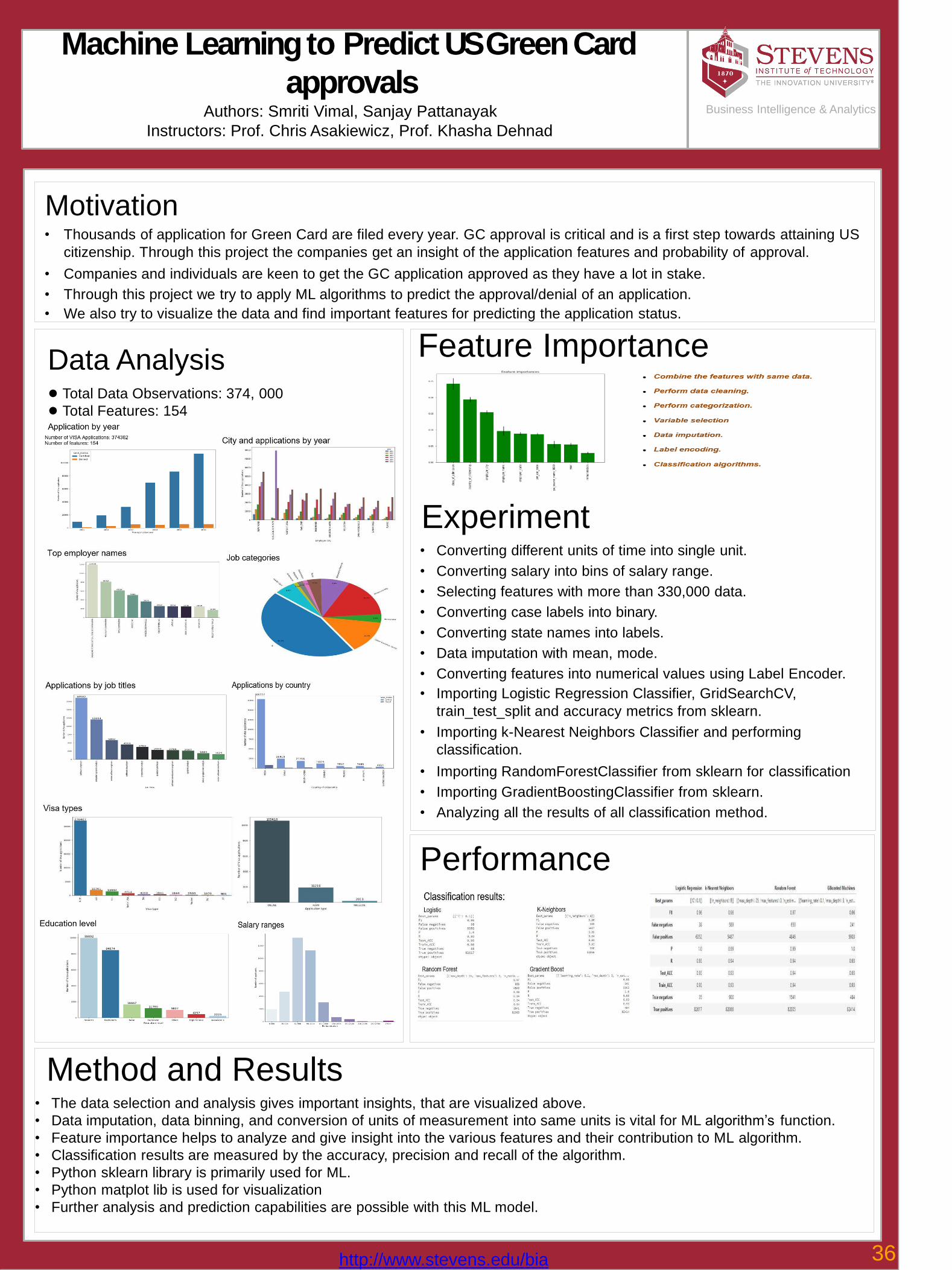
Machine Learning to Predict US GreenCard
approvalsAuthors: Smriti Vimal, Sanjay Pattanayak
Instructors: Prof. Chris Asakiewicz, Prof. Khasha Dehnad
Business Intelligence & Analytics
Motivation• Thousands of application for Green Card are filed every year. GC approval is critical and is a first step towards attaining US
citizenship. Through this project the companies get an insight of the application features and probability of approval.
• Companies and individuals are keen to get the GC application approved as they have a lot in stake.
• Through this project we try to apply ML algorithms to predict the approval/denial of an application.
• We also try to visualize the data and find important features for predicting the application status.
Data Analysis● Total Data Observations: 374, 000
● Total Features: 154
Performance
Method and Results• The data selection and analysis gives important insights, that are visualized above.
• Data imputation, data binning, and conversion of units of measurement into same units is vital for ML algorithm’s function.
• Feature importance helps to analyze and give insight into the various features and their contribution to ML algorithm.
• Classification results are measured by the accuracy, precision and recall of the algorithm.
• Python sklearn library is primarily used for ML.
• Python matplot lib is used for visualization
• Further analysis and prediction capabilities are possible with this ML model.
Feature Importance
Experiment• Converting different units of time into single unit.
• Converting salary into bins of salary range.
• Selecting features with more than 330,000 data.
• Converting case labels into binary.
• Converting state names into labels.
• Data imputation with mean, mode.
• Converting features into numerical values using Label Encoder.
• Importing Logistic Regression Classifier, GridSearchCV,
train_test_split and accuracy metrics from sklearn.
• Importing k-Nearest Neighbors Classifier and performing
classification.
• Importing RandomForestClassifier from sklearn for classification
• Importing GradientBoostingClassifier from sklearn.
• Analyzing all the results of all classification method.
36http://www.stevens.edu/bia
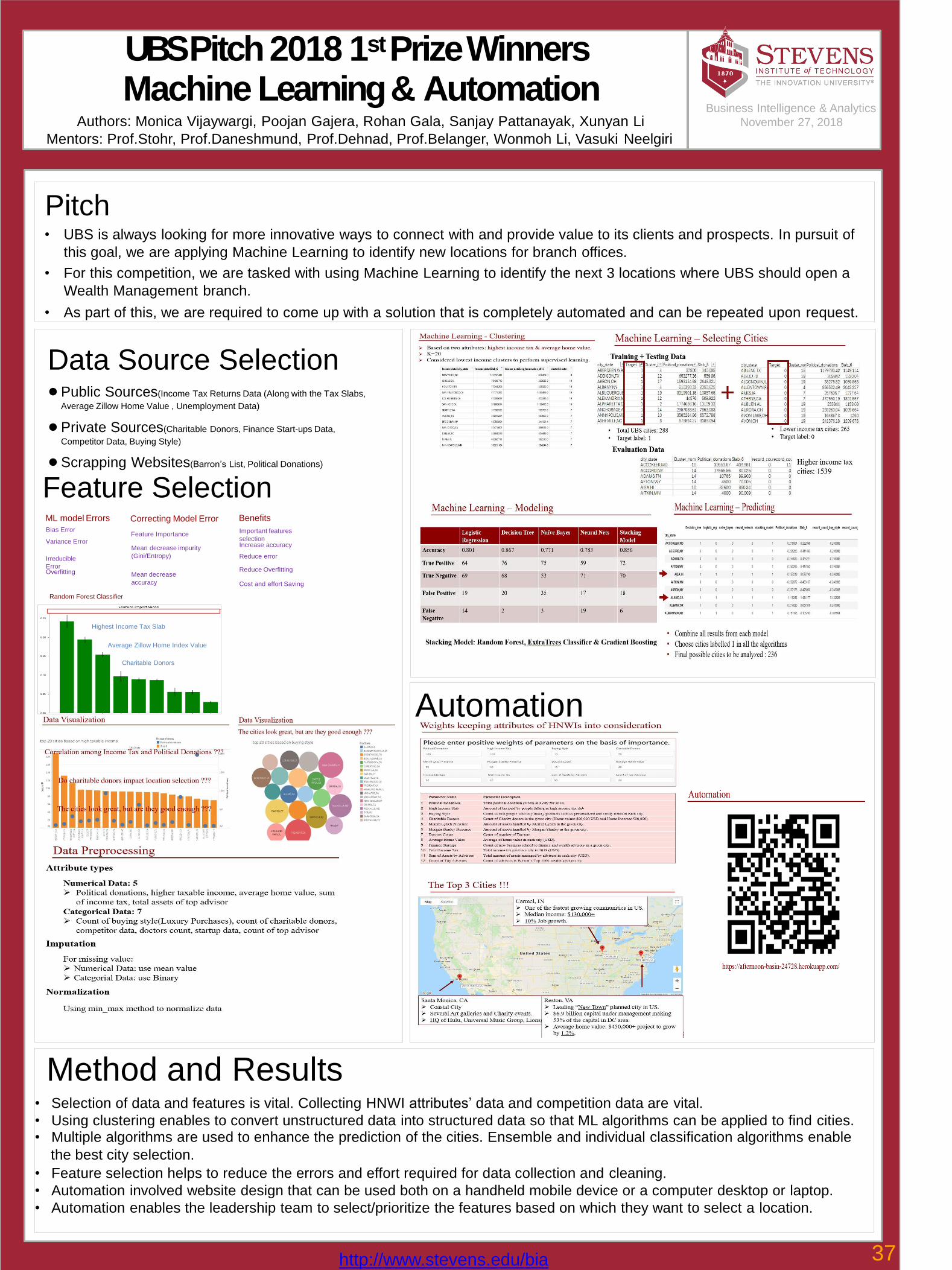
UBS Pitch 2018 1st PrizeWinnersMachine Learning & Automation
Authors: Monica Vijaywargi, Poojan Gajera, Rohan Gala, Sanjay Pattanayak, Xunyan Li
Mentors: Prof.Stohr, Prof.Daneshmund, Prof.Dehnad, Prof.Belanger, Wonmoh Li, Vasuki Neelgiri
Business Intelligence & Analytics
November 27, 2018
Pitch• UBS is always looking for more innovative ways to connect with and provide value to its clients and prospects. In pursuit of
this goal, we are applying Machine Learning to identify new locations for branch offices.
• For this competition, we are tasked with using Machine Learning to identify the next 3 locations where UBS should open a
Wealth Management branch.
• As part of this, we are required to come up with a solution that is completely automated and can be repeated upon request.
Automation
Method and Results• Selection of data and features is vital. Collecting HNWI attributes’ data and competition data are vital.
• Using clustering enables to convert unstructured data into structured data so that ML algorithms can be applied to find cities.• Multiple algorithms are used to enhance the prediction of the cities. Ensemble and individual classification algorithms enable
the best city selection.
• Feature selection helps to reduce the errors and effort required for data collection and cleaning.
• Automation involved website design that can be used both on a handheld mobile device or a computer desktop or laptop.
• Automation enables the leadership team to select/prioritize the features based on which they want to select a location.
Data Source Selection● Public Sources(Income Tax Returns Data (Along with the Tax Slabs,
Average Zillow Home Value , Unemployment Data)
● Private Sources(Charitable Donors, Finance Start-ups Data,
Competitor Data, Buying Style)
● Scrapping Websites(Barron’s List, Political Donations)
Feature SelectionML model Errors
Bias Error
Variance Error
Irreducible
Error Overfitting
Correcting Model Error
Feature Importance
Mean decrease impurity
(Gini/Entropy)
Mean decrease
accuracy
Benefits
Important features
selectionIncrease accuracy
Reduce error
Reduce Overfitting
Cost and effort Saving
Random Forest Classifier
Highest Income Tax Slab
Average Zillow Home Index Value
Charitable Donors
37http://www.stevens.edu/bia
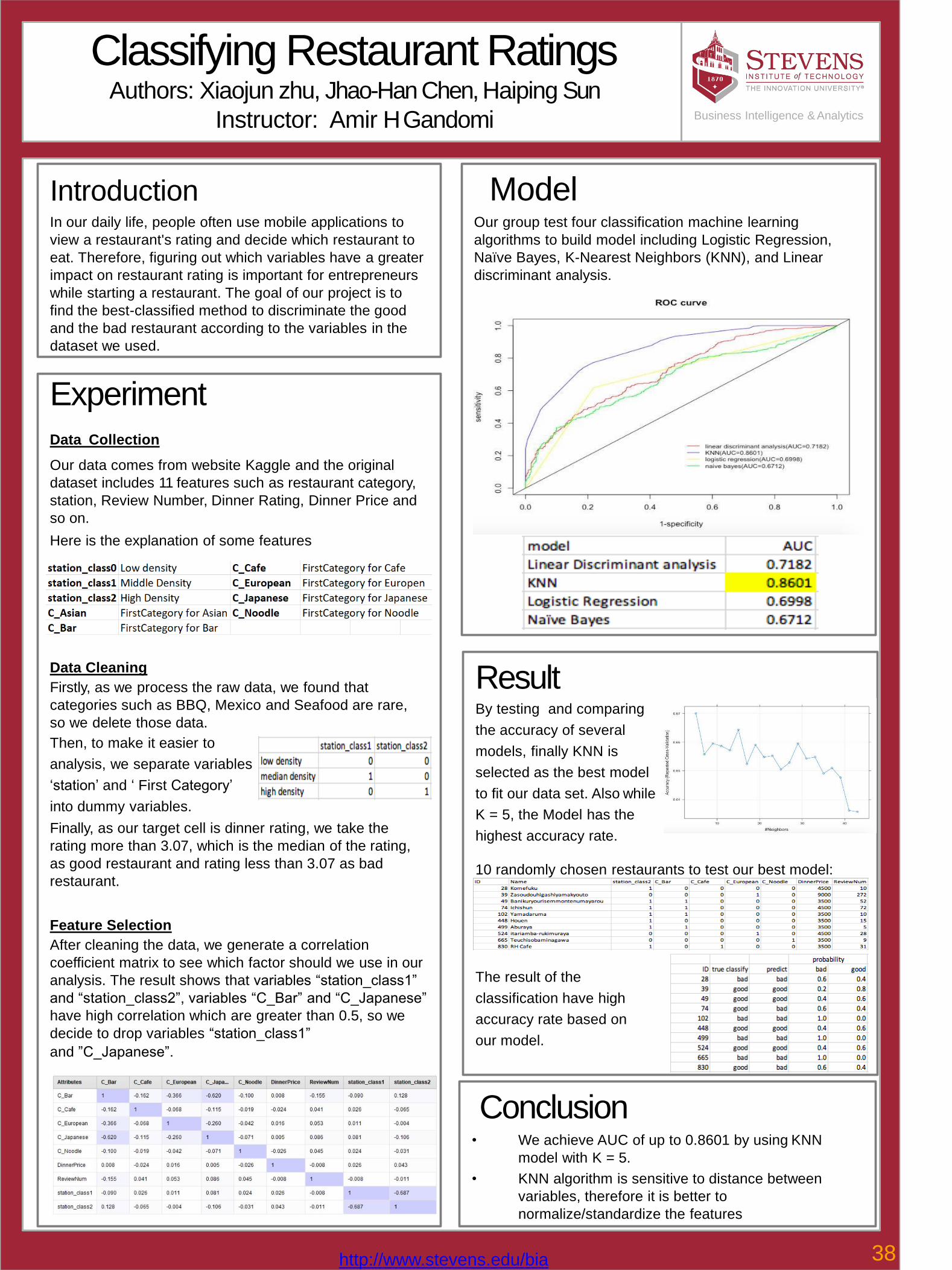
Classifying Restaurant RatingsAuthors: Xiaojun zhu, Jhao-Han Chen, Haiping Sun
Instructor: Amir HGandomi Business Intelligence & Analytics
IntroductionIn our daily life, people often use mobile applications to
view a restaurant's rating and decide which restaurant to
eat. Therefore, figuring out which variables have a greater
impact on restaurant rating is important for entrepreneurs
while starting a restaurant. The goal of our project is to
find the best-classified method to discriminate the good
and the bad restaurant according to the variables in the
dataset we used.
Conclusion• We achieve AUC of up to 0.8601 by using KNN
model with K = 5.
• KNN algorithm is sensitive to distance between
variables, therefore it is better to
normalize/standardize the features
ModelOur group test four classification machine learning
algorithms to build model including Logistic Regression,
Naïve Bayes, K-Nearest Neighbors (KNN), and Linear
discriminant analysis.
Experiment
Data Collection
Our data comes from website Kaggle and the original
dataset includes 11 features such as restaurant category,
station, Review Number, Dinner Rating, Dinner Price and
so on.
Here is the explanation of some features
Data Cleaning
Firstly, as we process the raw data, we found that
categories such as BBQ, Mexico and Seafood are rare,
so we delete those data.
Then, to make it easier to
analysis, we separate variables
‘station’ and ‘ First Category’
into dummy variables.
Finally, as our target cell is dinner rating, we take the
rating more than 3.07, which is the median of the rating,
as good restaurant and rating less than 3.07 as bad
restaurant.
Feature Selection
After cleaning the data, we generate a correlation
coefficient matrix to see which factor should we use in our
analysis. The result shows that variables “station_class1”
and “station_class2”, variables “C_Bar” and “C_Japanese”
have high correlation which are greater than 0.5, so we
decide to drop variables “station_class1”
and ”C_Japanese”.
ResultBy testing and comparing
the accuracy of several
models, finally KNN is
selected as the best model
to fit our data set. Also while
K = 5, the Model has the
highest accuracy rate.
10 randomly chosen restaurants to test our best model:
The result of the
classification have high
accuracy rate based on
our model.
38http://www.stevens.edu/bia
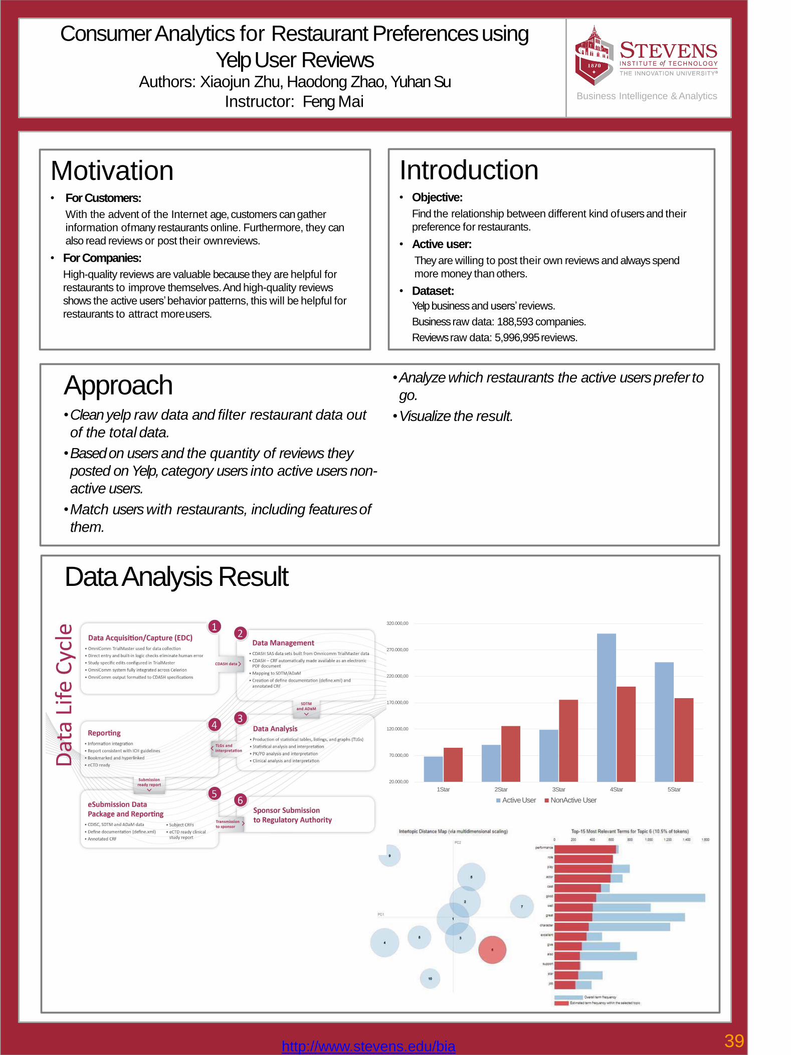
Consumer Analytics for Restaurant Preferencesusing
Yelp User ReviewsAuthors: Xiaojun Zhu, Haodong Zhao, Yuhan Su
Instructor: Feng Mai
Approach•Clean yelp raw data and filter restaurant data out
of the total data.
•Based on users and the quantity of reviews they
posted on Yelp, category users into active users non-
active users.
•Match users with restaurants, including featuresof
them.
•Analyze which restaurants the active users prefer to
go.
•Visualize the result.
Business Intelligence & Analytics
Motivation• For Customers:
With the advent of the Internet age, customers can gather
information ofmany restaurants online. Furthermore, they can
also read reviews or post their ownreviews.
• For Companies:
High-quality reviews are valuable because they are helpful for
restaurants to improve themselves. And high-quality reviews
shows the active users’ behavior patterns, this will be helpful for
restaurants to attract moreusers.
Introduction• Objective:
Find the relationship between different kind ofusers and their
preference for restaurants.
• Active user:
Theyare willing to post their own reviews and always spend
more money than others.
• Dataset:
Yelp business and users’ reviews.
Business raw data: 188,593 companies.
Reviews raw data: 5,996,995reviews.
Data Analysis Result
20.000,00
70.000,00
120.000,00
170.000,00
220.000,00
270.000,00
320.000,00
1Star 4Star 5Star2Star
ActiveUser
3Star
NonActive User
39http://www.stevens.edu/bia
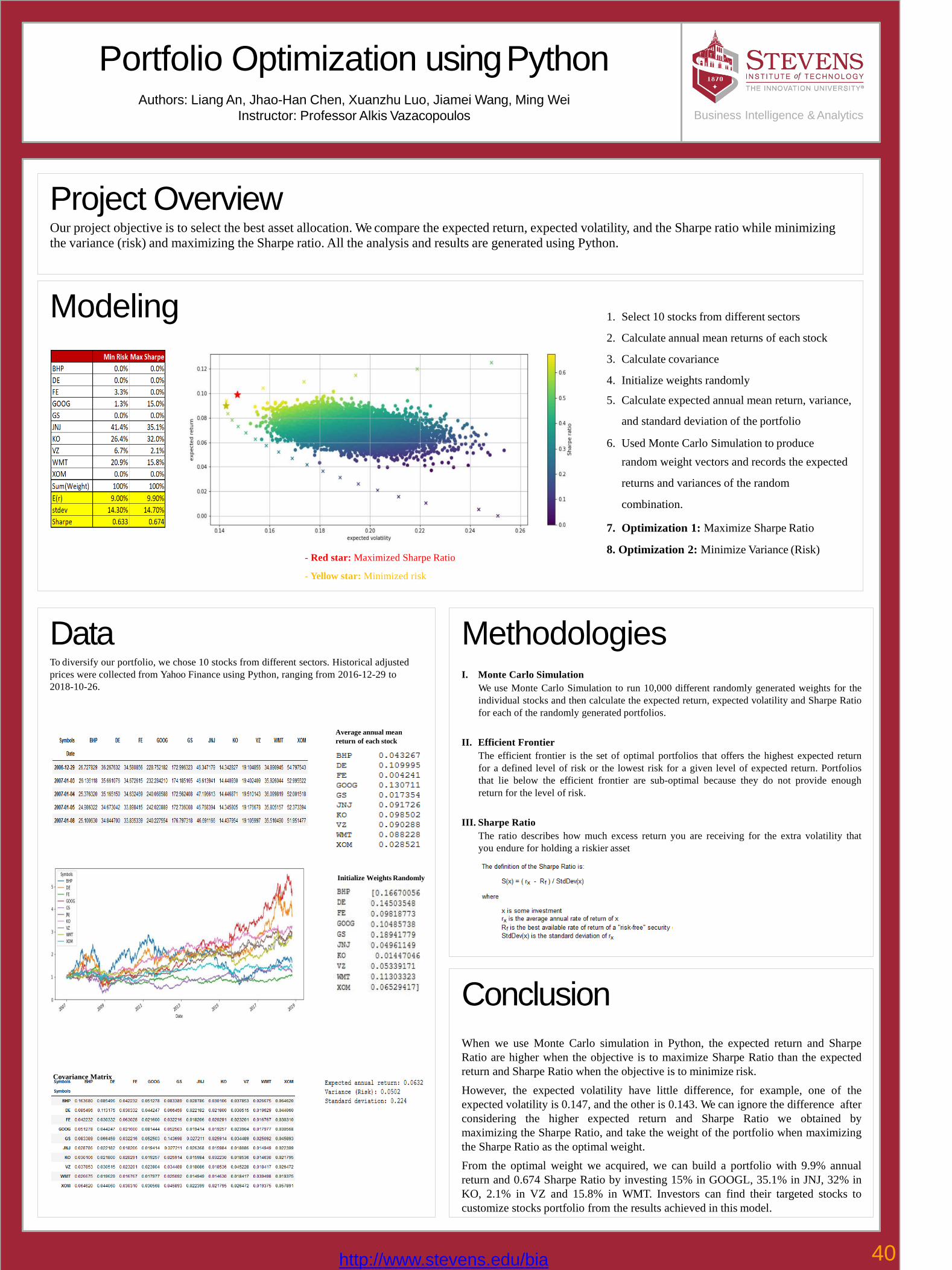
Portfolio Optimization usingPythonAuthors: Liang An, Jhao-Han Chen, Xuanzhu Luo, Jiamei Wang, Ming Wei
Instructor: Professor Alkis Vazacopoulos
Modeling
Project OverviewOur project objective is to select the best asset allocation. We compare the expected return, expected volatility, and the Sharpe ratio while minimizing
the variance (risk) and maximizing the Sharpe ratio. All the analysis and results are generated using Python.
MethodologiesI. Monte Carlo Simulation
We use Monte Carlo Simulation to run 10,000 different randomly generated weights for the
individual stocks and then calculate the expected return, expected volatility and Sharpe Ratio
for each of the randomly generated portfolios.
II. Efficient Frontier
The efficient frontier is the set of optimal portfolios that offers the highest expected return
for a defined level of risk or the lowest risk for a given level of expected return. Portfolios
that lie below the efficient frontier are sub-optimal because they do not provide enough
return for the level of risk.
III. Sharpe Ratio
The ratio describes how much excess return you are receiving for the extra volatility that
you endure for holding a riskier asset
Business Intelligence & Analytics
Conclusion
When we use Monte Carlo simulation in Python, the expected return and Sharpe
Ratio are higher when the objective is to maximize Sharpe Ratio than the expected
return and Sharpe Ratio when the objective is to minimize risk.
However, the expected volatility have little difference, for example, one of the
expected volatility is 0.147, and the other is 0.143. We can ignore the difference after
considering the higher expected return and Sharpe Ratio we obtained by
maximizing the Sharpe Ratio, and take the weight of the portfolio when maximizing
the Sharpe Ratio as the optimal weight.
From the optimal weight we acquired, we can build a portfolio with 9.9% annual
return and 0.674 Sharpe Ratio by investing 15% in GOOGL, 35.1% in JNJ, 32% in
KO, 2.1% in VZ and 15.8% in WMT. Investors can find their targeted stocks to
customize stocks portfolio from the results achieved in this model.
- Red star: Maximized Sharpe Ratio
- Yellow star: Minimized risk
1. Select 10 stocks from different sectors
2. Calculate annual mean returns of each stock
3. Calculate covariance
4. Initialize weights randomly
5. Calculate expected annual mean return, variance,
and standard deviation of the portfolio
6. Used Monte Carlo Simulation to produce
random weight vectors and records the expected
returns and variances of the random
combination.
7. Optimization 1: Maximize Sharpe Ratio
8. Optimization 2: Minimize Variance (Risk)
DataTo diversify our portfolio, we chose 10 stocks from different sectors. Historical adjusted
prices were collected from Yahoo Finance using Python, ranging from 2016-12-29 to
2018-10-26.
Average annual mean
return of each stock
Initialize Weights Randomly
Covariance Matrix
40http://www.stevens.edu/bia

Radiology Assistant
INSTRUCTOR: Dr. Christopher Asakiewicz AMIT
KUMAR | JAYESH MEHTA | YASH WANVE
OBJECTIVE: To create a model that recognizes different x-ray types by exposing them through an input
device.
INTRODUCTION:
Machine learning as a technology that has several
implementations and the scope of growth is beyond
current human comprehension. During our
research to choose a topic we came across an idea
in which we wanted to expose an X-ray copy to our
model through an input device and it would give an
output which would tell us whether the lungs are
infected with a disease or not.
DATA:
We derived our dataset online over which we
implemented our neural network to develop the
model. The dataset consists of multiple folders
with x-rays of different diseases segregated
accordingly.
MODELLING:
We have used Convoluted Neural Networks
(CNN) for analyzing our input i.e. x-ray images.
The CNN architectures make the assumption that
the inputs are images, which allows us to encode
certain properties into the architecture. These then
make the forward function more efficient to
implement and vastly reduce the amount of
parameters in the network.
We used 3 convolutional layers and 3 maxpooling
layers of 2x2 size in our CNN.
Our model experiences a log loss of 0.8 .
OPENCV:
We have utilized OpenCV library for computer
vision. We have used a camera as input device
through which
the x-ray images are fed.
RESULTS:
After training our model on the dataset we then fed a
sample x-ray from the input device and the program
generates an output which tells us whether the set of
lungs have contracted a disease or not and if yes,
then which disease would
it be.
The heatmap on
the output
image tells us about
the probability of
whether that
area is infected or
not. The green
patches on the
lower side of both the lungs show positiveprediction of an infection.
We tested some random x-ray to test the model.
Example : This image shows the symptoms of
effusion and when we tested it using our model we
also got the same result.
[0,1,0,0]
CONCLUSION
CNNs compare images piece by piece. The pieces
that it looks for are called features. By finding rough
feature matches in roughly the same positions in two
images, CNNs get a lot better at seeing41
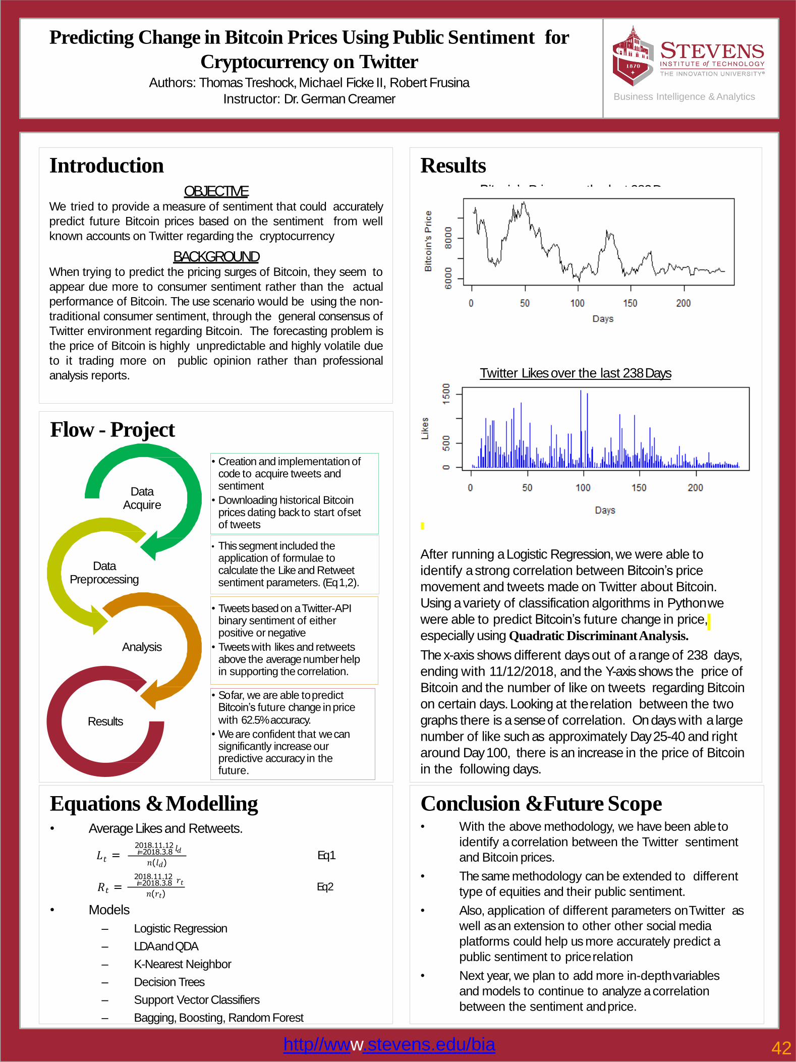
Predicting Change in Bitcoin Prices Using Public Sentiment for
Cryptocurrency on TwitterAuthors: Thomas Treshock, Michael Ficke II, Robert Frusina
Instructor: Dr. German Creamer
Bitcoin’s Price over the last 283Days
Results
Twitter Likes over the last 238Days
After running a Logistic Regression, we were able to
identify a strong correlation between Bitcoin’s price
movement and tweets made on Twitter about Bitcoin.
Using a variety of classification algorithms in Pythonwe
were able to predict Bitcoin’s future change in price,
especially using Quadratic DiscriminantAnalysis.
The x-axis shows different days out of a range of 238 days,
ending with 11/12/2018, and the Y-axis shows the price of
Bitcoin and the number of like on tweets regarding Bitcoin
on certain days. Looking at therelation between the two
graphs there is a sense of correlation. On days with a large
number of like such as approximately Day 25-40 and right
around Day 100, there is an increase in the price of Bitcoin
in the following days.
IntroductionOBJECTIVE
We tried to provide a measure of sentiment that could accurately
predict future Bitcoin prices based on the sentiment from well
known accounts on Twitter regarding the cryptocurrency
BACKGROUNDWhen trying to predict the pricing surges of Bitcoin, they seem to
appear due more to consumer sentiment rather than the actual
performance of Bitcoin. The use scenario would be using the non-
traditional consumer sentiment, through the general consensus of
Twitter environment regarding Bitcoin. The forecasting problem is
the price of Bitcoin is highly unpredictable and highly volatile due
to it trading more on public opinion rather than professional
analysis reports.
Business Intelligence & Analytics
http//www.stevens.edu/bia
Flow - Project
Conclusion & Future Scope• With the above methodology, we have been ableto
identify a correlation between the Twitter sentiment
and Bitcoin prices.
• The same methodology can be extended to different
type of equities and their public sentiment.
• Also, application of different parameters onTwitter as
well as an extension to other other social media
platforms could help us more accurately predict a
public sentiment to pricerelation
• Next year, we plan to add more in-depthvariables
and models to continue to analyze a correlation
between the sentiment andprice.
Equations &Modelling• Average Likes and Retweets.
𝑡𝐿 =2018.11.12 𝑙𝑑𝑖=2018.3.8
𝑛(𝑙𝑑)
𝑡
Eq1
𝑅 =𝑟𝑡
2018.11.12𝑖=2018.3.8
𝑛(𝑟𝑡)Eq2
• Models
– Logistic Regression
– LDA andQDA
– K-Nearest Neighbor
– Decision Trees
– Support Vector Classifiers
– Bagging, Boosting, Random Forest
• Creation and implementation of code to acquire tweets and sentiment
• Downloading historical Bitcoin prices dating back to start ofset of tweets
Data Acquire
• This segment included the application of formulae to calculate the Like and Retweet sentiment parameters. (Eq1,2).
Data Preprocessing
• Tweets based on a Twitter-API binary sentiment of either positive or negative
• Tweets with likes and retweets above the average numberhelp in supporting thecorrelation.
Analysis
• So far, we are able topredictBitcoin’s future change inpricewith 62.5%accuracy.
• We are confident that wecan significantly increase our predictive accuracy in the future.
Results
42

Surface-Enhancement Raman Scattering of Urine
Samples for Risk Assessment of Prostate CancerAuthors: Yiwei Ma, Yanbo Wang, Guohao Gao
Instructor: Prof. Amir H Gandomi, Ph.D.
https://www.stevens.edu/bia
Introduction
➢ Prostate cancer is the most commonly diagnosed non-cutaneous cancer in men
in the US, with approximately 1 in 6 men will be diagnosed with prostate cancer at
some point in their lives.
➢ Not all cancers are equal since prostate cancer is heterogeneous and can follow
multiple paths. An indolent case is induced that can cause no harm during
patients’ lifetime.
➢ PSA (prostate specific antigen) level cannot predict prostate cancer with high
degree of accuracy.
➢ This discriminant of biomarker(s) will further increase the accuracy of the
current prediction of tumor aggressiveness, and guide physicians to
choose a safe approach, increase the survival rate.
➢ Decrease the possibility of leading overtreatment and avoids the risk in
both economical cost and long-lasting side effects.
➢ The method identifies the novel biomarker(s) also can be applied in other
disease treatment which is closely related with the urethra system.
Our Methods
➢
➢
Research Objectives
We hypothesize that SERS can be utilized to detect biomarker(s) in the
urine of prostate cancer patients that could serve as an indicator of
severity of cancer.
Statistical analysis method, PCA-LDA, can be applied into differentiate
SERS spectra of indolent and lethal cases.
➢ Carrying out SERS investigation of
banked urine specimens from two
groups of prostate cancer patients.
Group A–low risk, indolent cases.
Group B–high risk, lethal cases.
Impact Statement
Overview
➢ New and novel approaches that will enable clinicians to differentiate indolent and lethal prostate cancer so as to
aggressively treat only the latter type.
➢ Distinguishing the indolent cases from the minority of lethal ones in order to minimize overtreatment intervention.
Current Results
➢ Conducting principle component
analysis (PCA) and linear
discriminant analysis (LDA) of
SERS spectra for classification.
➢ the SERS findings and clinicalEstablishing the correlation between
outcome of the prostate cancer.
➢ SERS spectra of indolent and lethal cases.
➢ The scatter plot of LDA of binary classifications after PCA-LDA treatment.
500 1000 1500 2000
55000
110000
165000
220000
275000
Raman Shift (cm-1)
Indolent Group
500 1000 2000 2500
79000
158000
237000
316000
395000
Lethal ou
Gr p
1500
Raman Shift (cm-1)
Inte
ns
ity
(a.u
.)
0 20 100 120
-1.0
-0.8
-0.6
-0.4
-0.2
0.0
0.2
0.4
Indolent
Lethal
Dis
cri
min
an
tS
co
re
s
40 60 80
Samplenumbers
500 2000-20000
0
140000
160000
Inte
nsit
y (
a.u
.) In
ten
sit
y(a
.u.)
1000 1500
Raman Shift (cm-1)
Indolent
Lethal
Indolent-Lethal
1
1133
638
120000
100000
777
603
80000
60000
40000
20000
➢ 20 urine samples are analyzed, 16
in the indolent group and 4 in the
lethal group. For each sample, the
SERS measurement is repeated 6
times. In total, 120 SERS spectra
are acquired and used.
➢ PCA is used to visualize the
variances between groups with
corresponding to score plots. PCs
with higher associations with their
class identities are preferentially
used in LDA to achieve a better
classification performance.
Urine sample Ag nanoparticles colloidal solution
Mixture
He-Ne
Laser
(632.8 nm)
-2000000 0-1500000
-1000000
-500000
0
500000
1000000
Indolent
Lethal
PC
2(2
.7%
)
2000000 4000000 6000000 8000000
PC1(94.6%)
-1500000 -1000000 -500000 0 500000 1000000
-800000
-600000
-400000
-200000
0
200000
400000
600000
800000 Indolent
Lethal
PC
3(1
.3%
)
PC2(2.7%)
-2000000 0
-800000
-600000
-400000
-200000
0
200000
400000
600000
800000 Indolent
Lethal
PC
3(1
.3%
)
2000000 4000000 6000000 8000000
PC1(94.6%)
43
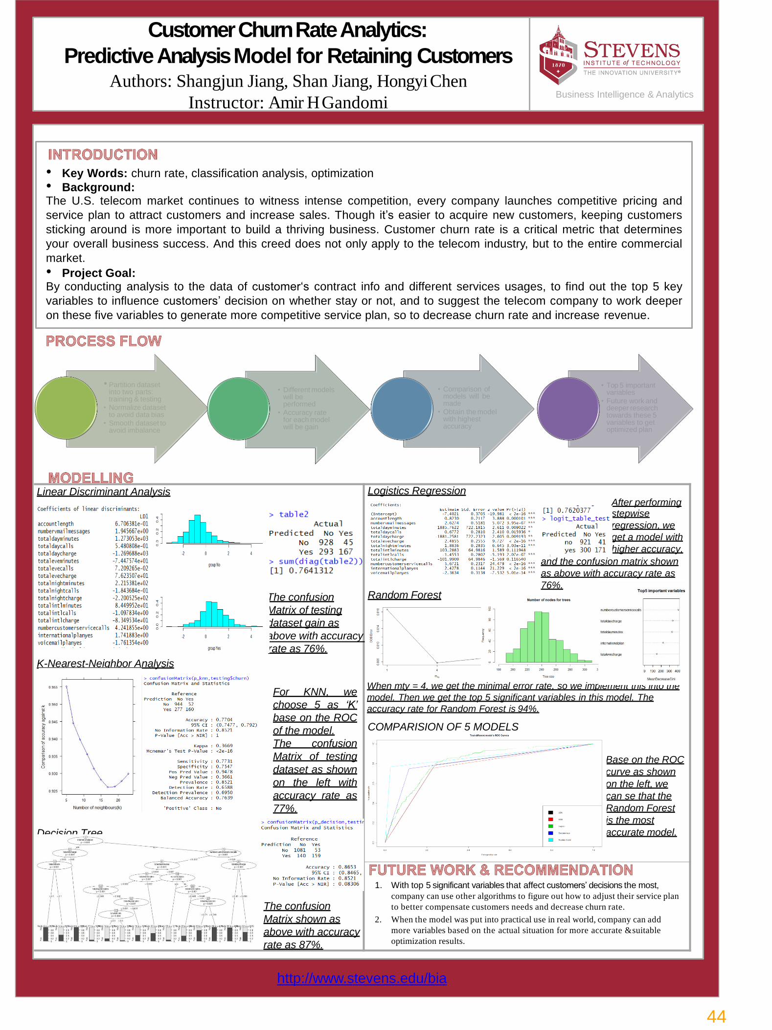
Customer Churn Rate Analytics:
Predictive Analysis Model for Retaining CustomersAuthors: Shangjun Jiang, Shan Jiang, HongyiChen
Instructor: Amir HGandomiBusiness Intelligence & Analytics
• Key Words: churn rate, classification analysis, optimization
• Background:The U.S. telecom market continues to witness intense competition, every company launches competitive pricing and
service plan to attract customers and increase sales. Though it’s easier to acquire new customers, keeping customers
sticking around is more important to build a thriving business. Customer churn rate is a critical metric that determines
your overall business success. And this creed does not only apply to the telecom industry, but to the entire commercial
market.
• Project Goal:By conducting analysis to the data of customer‘s contract info and different services usages, to find out the top 5 key
variables to influence customers’ decision on whether stay or not, and to suggest the telecom company to work deeper
on these five variables to generate more competitive service plan, so to decrease churn rate and increase revenue.
• Partition dataset into two parts: training & testing
• Normalize dataset to avoid data bias
• Smooth dataset to avoid imbalance
DATA WRANGLING
• Different models will be performed
• Accuracy rate for each model will be gain
EXPLORATORY DATA
ANALYSIS
• Comparison ofmodels will bemade
• Obtain the model with highest accuracy
OPTIMAZION
• Top 5 important variables
• Future work and deeper research towards these 5 variables to get optimized plan
CONSLUSION
http://www.stevens.edu/bia
Linear Discriminant Analysis
The confusion
Matrix of testing
dataset gain as
above with accuracy
Logistics RegressionAfter performingstepwise
regression, we
get a model with
higher accuracy,
and the confusion matrix shown
as above with accuracy rate as
76%.Random Forest
When mty = 4, we get the minimal error rate, so we implement this into the
model. Then we get the top 5 significant variables in this model. The
accuracy rate for Random Forest is 94%.
COMPARISION OF 5 MODELS
Base on the ROC
curve as shown
on the left, we
can se that the
Random Forest
is the most
accurate model.
rate as 76%.
K-Nearest-Neighbor Analysis
For KNN, we
choose 5 as ‘K’
base on the ROC
of the model.
The confusion
Matrix of testing
dataset as shown
on the left with
accuracy rate as
77%.
Decision Tree
The confusion
Matrix shown as
above with accuracy
rate as 87%.
1. With top 5 significant variables that affect customers’ decisions the most,
company can use other algorithms to figure out how to adjust their service plan
to better compensate customers needs and decrease churn rate.
2. When the model was put into practical use in real world, company can add
more variables based on the actual situation for more accurate & suitable
optimization results.
44
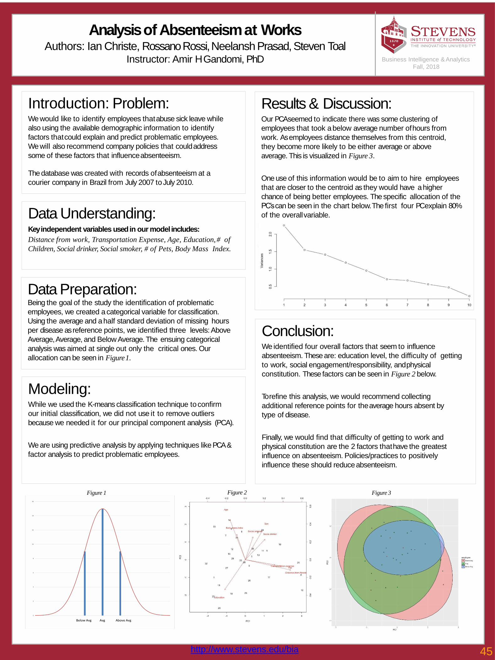
Analysis of Absenteeism at WorksAuthors: Ian Christe, Rossano Rossi, Neelansh Prasad, Steven Toal
Instructor: Amir H Gandomi, PhD
Results & Discussion:Our PCA seemed to indicate there was some clustering of
employees that took a below average number ofhours from
work. As employees distance themselves from this centroid,
they become more likely to be either average or above
average. This is visualized in Figure 3.
One use of this information would be to aim to hire employees
that are closer to the centroid as they would have a higher
chance of being better employees. The specific allocation of the
PC’s can be seen in the chart below.The first four PC explain 80%
of the overallvariable.
Introduction: Problem:We would like to identify employees thatabuse sick leave while
also using the available demographic information to identify
factors thatcould explain and predict problematic employees.
We will also recommend company policies that couldaddress
some of these factors that influenceabsenteeism.
The database was created with records ofabsenteeism at a
courier company in Brazil from July 2007 toJuly 2010.
Modeling:While we used the K-means classification technique toconfirm
our initial classification, we did not use it to remove outliers
because we needed it for our principal component analysis (PCA).
We are using predictive analysis by applying techniques likePCA &
factor analysis to predict problematic employees.
Conclusion:We identified four overall factors that seem to influence
absenteeism. These are: education level, the difficulty of getting
to work, social engagement/responsibility, andphysical
constitution. These factors can be seen in Figure 2 below.
To refine this analysis, we would recommend collecting
additional reference points for theaverage hours absent by
type of disease.
Finally, we would find that difficulty of getting to work and
physical constitution are the 2 factors thathave the greatest
influence on absenteeism. Policies/practices to positively
influence these should reduceabsenteeism.
Business Intelligence & Analytics
Fall, 2018
Data Understanding:Key independent variables used in our model includes:
Distance from work, Transportation Expense, Age, Education, # of
Children, Social drinker, Social smoker, # of Pets, Body Mass Index.
Data Preparation:Being the goal of the study the identification of problematic
employees, we created a categorical variable for classification.
Using the average and a half standard deviation of missing hours
per disease as reference points, we identified three levels: Above
Average, Average, and Below Average. The ensuing categorical
analysis was aimed at single out only the critical ones. Our
allocation can be seen in Figure1.
Figure 1 Figure 2 Figure 3
http://www.stevens.edu/bia 45
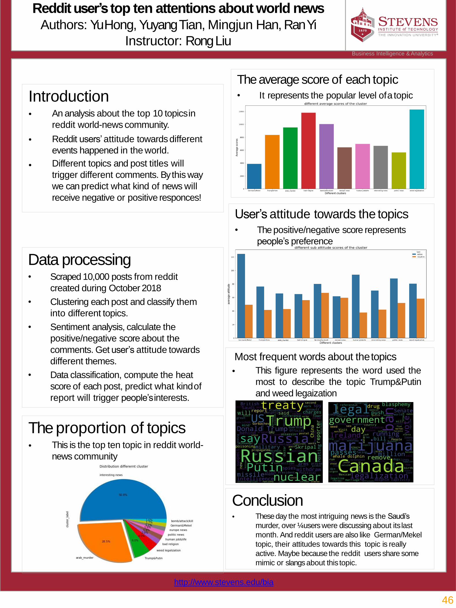
Reddit user’s top ten attentions about world news Authors: Yu Hong, Yuyang Tian, Mingjun Han, Ran Yi
Instructor: RongLiu
The average score of each topic• It represents the popular level ofa topicIntroduction
•
•
•
An analysis about the top 10 topicsin
reddit world-news community.
Reddit users’ attitude towardsdifferent
events happened in the world.
Different topics and post titles will
trigger different comments. By this way
we can predict what kind of news will
receive negative or positive responces!
Data processing• Scraped 10,000 posts from reddit
created during October 2018
• Clustering each post and classify them
into different topics.
• Sentiment analysis, calculate the
positive/negative score about the
comments. Get user’s attitude towards
different themes.
• Data classification, compute the heat
score of each post, predict what kindof
report will trigger people’sinterests.
Conclusion• These day the most intriguing news is the Saudi’s
murder, over ¼users were discussing about its last
month. And reddit users are also like German/Mekel
topic, their attitudes towards this topic is really
active. Maybe because the reddit users share some
mimic or slangs about this topic.
Business Intelligence & Analytics
The proportion of topics• This is the top ten topic in reddit world-
news community
Most frequent words about thetopics
• This figure represents the word used the
most to describe the topic Trump&Putin
and weed legaization
User’s attitude towards the topics• The positive/negative score represents
people’s preference
http://www.stevens.edu/bia
46
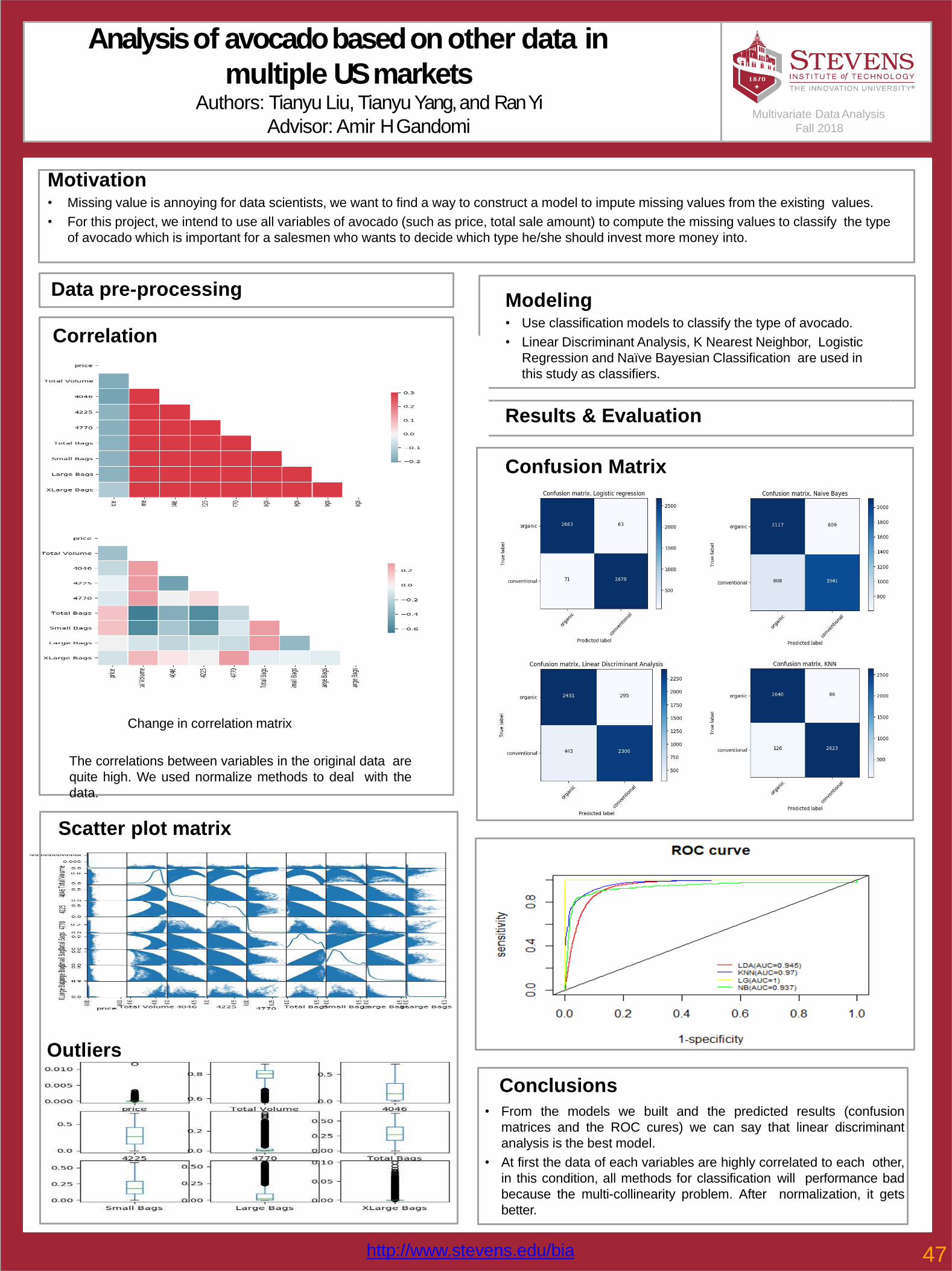
Analysis of avocado based on other data in
multiple USmarketsAuthors: Tianyu Liu, Tianyu Yang, and Ran Yi
Advisor: Amir HGandomi
Results & Evaluation
Motivation• Missing value is annoying for data scientists, we want to find a way to construct a model to impute missing values from the existing values.
• For this project, we intend to use all variables of avocado (such as price, total sale amount) to compute the missing values to classify the type
of avocado which is important for a salesmen who wants to decide which type he/she should invest more money into.
Modeling• Use classification models to classify the type of avocado.
• Linear Discriminant Analysis, K Nearest Neighbor, Logistic
Regression and Naïve Bayesian Classification are used in
this study as classifiers.
Multivariate Data Analysis
Fall 2018
Data pre-processing
Correlation
Change in correlation matrix
The correlations between variables in the original data are
quite high. We used normalize methods to deal with the
data.
Scatter plot matrix
Outliers
ROC curve
Confusion Matrix
Conclusions
• From the models we built and the predicted results (confusion
matrices and the ROC cures) we can say that linear discriminant
analysis is the best model.
• At first the data of each variables are highly correlated to each other,
in this condition, all methods for classification will performance bad
because the multi-collinearity problem. After normalization, it gets
better.
http://www.stevens.edu/bia 47
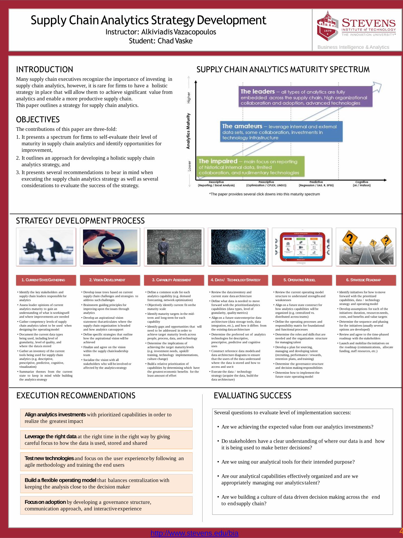
Supply ChainAnalytics Strategy DevelopmentInstructor: AlkiviadisVazacopoulos
Student: ChadVaskeBusiness Intelligence & Analytics
INTRODUCTIONMany supply chain executives recognize the importance of investing in
supply chain analytics, however, it is rare for firms to have a holistic
strategy in place that will allow them to achieve significant value from
analytics and enable a more productive supply chain.
This paper outlines a strategy for supply chain analytics.
OBJECTIVESThe contributions of this paper are three-fold:
1. It presents a spectrum for firms to self-evaluate their level of
maturity in supply chain analytics and identify opportunities for
improvement,
2. It outlines an approach for developing a holistic supply chain
analytics strategy, and
3. It presents several recommendations to bear in mind when
executing the supply chain analytics strategy as well as several
considerations to evaluate the success of the strategy.
1. CURRENT STATEGATHERING 2. VISIONDEVELOPMENT 3. CAPABILITY ASSESSMENT 5. OPERATINGMODEL4. DATA / TECHNOLOGYSTRATEGY 6. STRATEGICROADMAP
• Identify the key stakeholders and
supply chain leaders responsible for
analytics
• Assess leader opinions of current
analytics maturity to gain an
understanding of what is workingwell
and where improvements are needed
• Gather competency levels of supply
chain analytics talent to be used when
designing the operating model
• Document the current data types
being used, including level of
granularity, level of quality, and
where the data is stored
• Gather an inventory of the current
tools being used for supply chain
analytics (e.g. descriptive,
prescriptive, predictive, cognitive,
visualization)
• Summarize themes from the current
state to keep in mind while building
the analytics strategy
• Develop issue trees based on current
supply chain challenges and strategies to
address such challenges
• Brainstorm guiding principles for
improving upon the issues through
analytics
• Develop an aspirational vision
statement thatarticulates where the
supply chain organization is headed
and how analytics cansupport
• Define specific strategies that outline
how the aspirational vision will be
achieved
• Finalize and agree on the vision
within the supply chain leadership
team
• Socialize the vision with all
stakeholders who will be involved or
affected by the analytics strategy
• Define a common scale for each
analytics capability (e.g. demand
forecasting, network optimization)
• Objectively identify current fit onthe
maturity scale
• Identify maturity targets in the mid-
term and long-term for each
capability
• Identify gaps and opportunities that will
need to be addressed in order to
achieve target maturity levels across
people, process, data, and technology
• Determine the implications of
achieving the target maturity levels
(e.g. investment needs, upskill/
training, technology implementations,
culture change)
• Build a relative prioritization of
capabilities by determining which have
the greatest economic benefits for the
least amount of effort
• Review the data inventory and
current state data architecture
• Define what data is needed to move
forward with the prioritizedanalytics
capabilities (data types, level of
granularity, quality metrics)
• Align on a future stateenterprise data
architecture (data storage tools, data
integration, etc.), and how it differs from
the existing data architecture
• Determine the preferred set of analytics
technologies for descriptive,
prescriptive, predictive and cognitive
uses
• Construct reference data models and
data architecture diagrams to ensure
that the users of the data understand
where the data is stored and how to
access and use it
• Execute the data / technology
strategy (acquire the data, build the
data architecture)
• Review the current operating model
structure to understand strengths and
weaknesses
• Align on a future state construct for
how analytics capabilities will be
organized (e.g. centralized vs.
distributed across teams)
• Define the operating processes and
responsibility matrix for foundational
and functional processes
• Determine the roles and skills that are
needed and the organization structure
for managing talent
• Develop a plan for sourcing,
managing and developing talent
(recruiting, performance / rewards,
retention plans, and training)
• Determine the governance structure
and decision making responsibilities
• Determine how to implement the
future state operating model
• Identify initiatives for how to move
forward with the prioritized
capabilities, data / technology
strategy and operating model
• Develop assumptions for each of the
initiatives: duration, resources needs,
costs, and benefits and value targets
• Determine the sequence and phasing
for the initiatives (usually several
options are developed)
• Review and agree to the time-phased
roadmap with the stakeholders
• Launch and mobilize the initiatives on
the roadmap (communications, allocate
funding, staff resources, etc.)
STRATEGY DEVELOPMENTPROCESS
EXECUTION RECOMMENDATIONS
Align analytics investments with prioritized capabilities in order to
realize the greatest impact
Leverage the right data at the right time in the right way by giving
careful focus to how the data is used, stored and shared
Test new technologies and focus on the user experience by following an
agile methodology and training the end users
Build a flexible operating model that balances centralization with
keeping the analysis close to the decision maker
Focus on adoption by developing a governance structure,
communication approach, and interactiveexperience
Several questions to evaluate level of implementation success:
• Are we achieving the expected value from our analytics investments?
• Do stakeholders have a clear understanding of where our data is and how
it is being used to make better decisions?
• Are we using our analytical tools for their intended purpose?
• Are our analytical capabilities effectively organized and are we
appropriately managing our analytics talent?
• Are we building a culture of data driven decision making across the end
to endsupply chain?
EVALUATING SUCCESS
SUPPLY CHAIN ANALYTICS MATURITY SPECTRUM
*The paper provides several click downs into this maturity spectrum
http://www.stevens.edu/bia 48
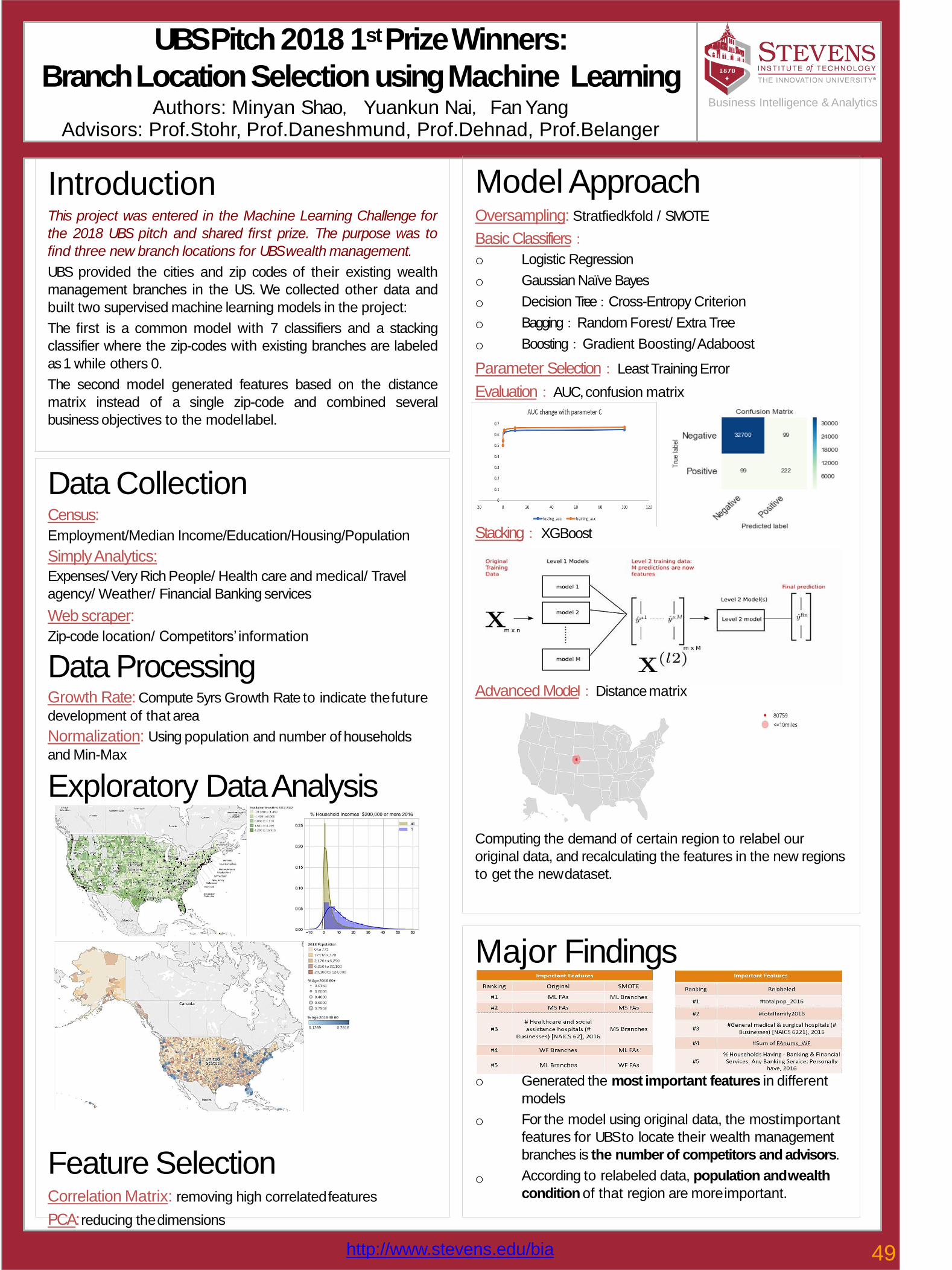
UBS Pitch 2018 1st PrizeWinners:
Branch Location Selection using Machine LearningAuthors: Minyan Shao,Yuankun Nai,Fan Yang
Advisors: Prof.Stohr, Prof.Daneshmund, Prof.Dehnad, Prof.Belanger
Model ApproachOversampling: Stratfiedkfold / SMOTE
Basic Classifiers:
o
o
o
o
o
Logistic Regression
Gaussian Naïve Bayes
Decision Tree:Cross-Entropy Criterion
Bagging:Random Forest/ Extra Tree
Boosting:Gradient Boosting/Adaboost
Parameter Selection:Least TrainingError
Evaluation:AUC, confusion matrix
Stacking:XGBoost
Advanced Model:Distancematrix
Computing the demand of certain region to relabel our
original data, and recalculating the features in the new regions
to get the newdataset.
IntroductionThis project was entered in the Machine Learning Challenge for
the 2018 UBS pitch and shared first prize. The purpose was to
find three new branch locations for UBSwealth management.
UBS provided the cities and zip codes of their existing wealth
management branches in the US. We collected other data and
built two supervised machine learning models in the project:
The first is a common model with 7 classifiers and a stacking
classifier where the zip-codes with existing branches are labeled
as1 while others 0.
The second model generated features based on the distance
matrix instead of a single zip-code and combined several
business objectives to the modellabel.
Data CollectionCensus:
Employment/Median Income/Education/Housing/Population
SimplyAnalytics:
Expenses/ Very Rich People/ Health care and medical/ Travel
agency/ Weather/ Financial Banking services
Web scraper:
Zip-code location/ Competitors’ information
Data ProcessingGrowth Rate: Compute 5yrs Growth Rate to indicate thefuture
development of that area
Normalization: Using population and number of households
and Min-Max
Exploratory DataAnalysis
Feature SelectionCorrelation Matrix: removing high correlatedfeatures
PCA: reducing thedimensions
Major Findings
o
o
o
Generated the most important features in different
models
For the model using original data, the mostimportant
features for UBS to locate their wealth management
branches is the number of competitors and advisors.
According to relabeled data, population andwealth
condition of that region are moreimportant.
Business Intelligence & Analytics
http://www.stevens.edu/bia 49

Predicting Overall Health from Behavioral Risk Factor
Surveillance Survey DataAuthors: Malik Mubeen and ErikaDeckter
Instructor: Amir H.Gandomi
ProblemStatement
•
•
•
•
•
The Centers for Disease Control and
Prevention performs an annualhealth
survey via telephone.
Data from the 2015 survey conducted in
New York State have been used to build a
prediction model to determine overall
health of the surveyrespondents
Data Reference:
https://health.data.ny.gov/Health/Behaviora
l-Risk-Factor-Surveillance-Survey-2015/rcr8-
b3jj
The data contain 12,357 survey responses.
Overall health is classified as either “Pooror
Fair Health” or “Good or BetterHealth.”
Multivariate Data Analytics
Fall 2018
DataPreparation
•
•
•
•
Survey responses without a overall health
class value were removed from the data(67
rows).
In general, unknown values for each variable
were replaced with the most common value
for eachresponse
Continuous variables were capped at a
reasonable maximum value, andmissing
values were replaced by the mean
The data set was divided into trainingdata
(75%) and test data (25%)
Results & Evaluation
Sensitivity of Model Accuracy to K for K-Nearest
Neighbor Model
Principal ComponentAnalysis
Classification Model Comparison
Accuracy Rate by Classification
Sensitivity vs. Specificity for Various ClassificationModels
Using Kaiser’s
Rule, dimensions
can be reduced to
38 principal
components
(versus 77
original variables)
Approximately a
50%reduction
The first 38
principal
components
explain 71%
of the total
variance
Classification
LogisticRegression
(LR)
LinearDiscriminant
Analys
is
(LDA)
NaïveBayes
K-Nearest
Neighbo
rs (K =
6)
K-Nearest
Neighbo
rs (K =
15)
Fair orPoor Health
Accuracy Rate 72.6% 71.7% 71.7% 69.6% 65.4%
Good or BetterHealth
Accuracy Rate 77.7% 78.2% 78.2% 66.7% 74.3%
Overall
Accuracy Rate 76.8% 77.1% 75.2% 67.3% 72.8%
http://www.stevens.edu/bia 50
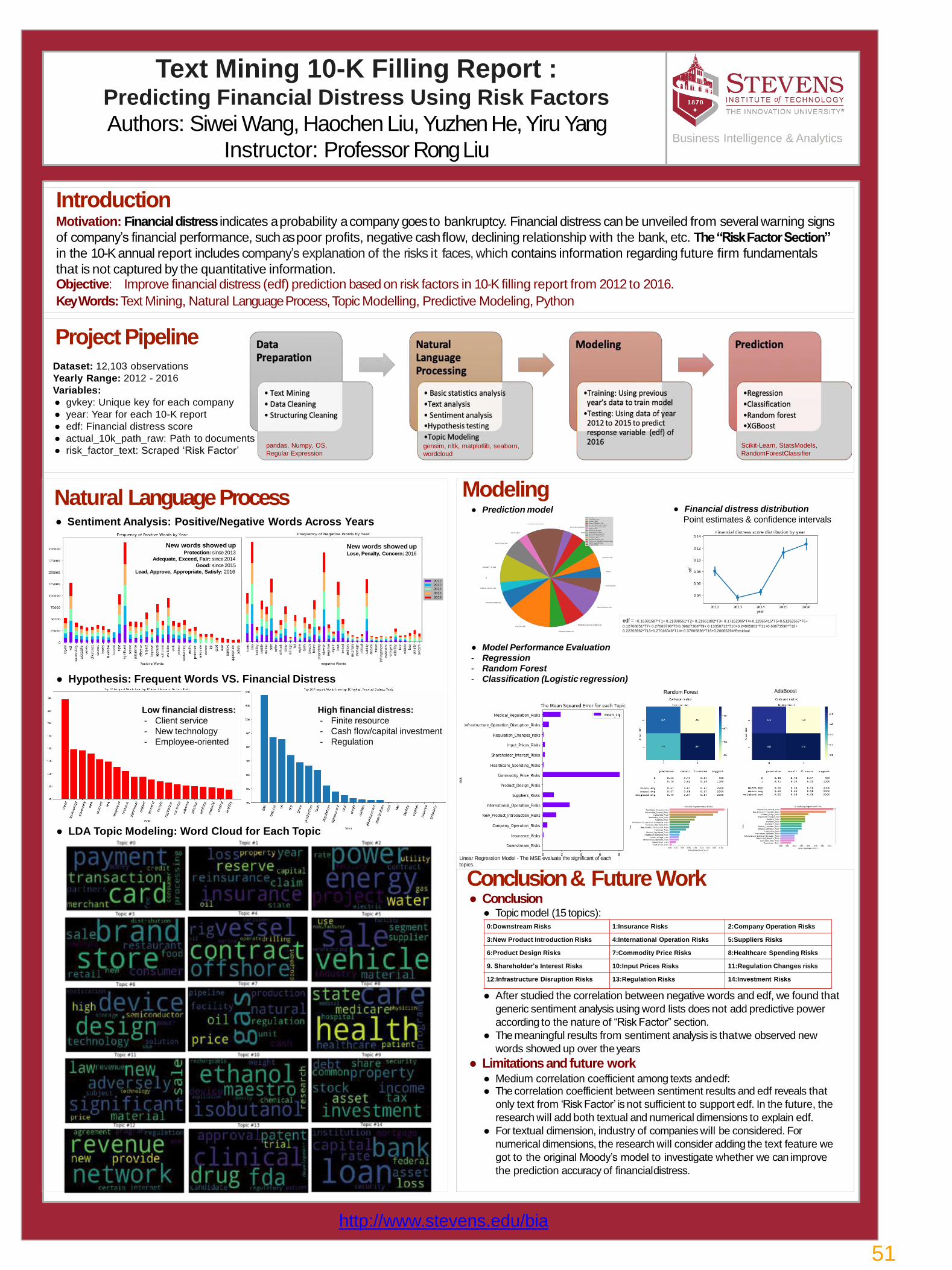
Text Mining 10-K Filling Report : Predicting Financial Distress Using Risk Factors
Authors: Siwei Wang, Haochen Liu, Yuzhen He, Yiru Yang
Instructor: Professor RongLiu
● Model Performance Evaluation
- Regression
- Random Forest
- Classification (Logistic regression)
IntroductionMotivation: Financial distress indicates a probability a company goes to bankruptcy. Financial distress can be unveiled from several warning signs
of company’s financial performance, such as poor profits, negative cash flow, declining relationship with the bank, etc. The “Risk Factor Section”
in the 10-K annual report includes company’s explanation of the risks it faces, which contains information regarding future firm fundamentals
that is not captured by the quantitative information.Objective: Improve financial distress (edf) prediction based on risk factors in 10-K filling report from 2012 to 2016.
Key Words: Text Mining, Natural Language Process, Topic Modelling, Predictive Modeling, Python
● After studied the correlation between negative words and edf, we found that
generic sentiment analysis using word lists does not add predictive power
according to the nature of “Risk Factor” section.
● The meaningful results from sentiment analysis is thatwe observed new
words showed up over theyears
● Limitations and future work● Medium correlation coefficient among texts andedf:● The correlation coefficient between sentiment results and edf reveals that
only text from ‘Risk Factor’ is not sufficient to support edf. In the future, the
research will add both textual and numerical dimensions to explain edf.
● For textual dimension, industry of companies will be considered. For
numerical dimensions, the research will consider adding the text feature we
got to the original Moody’s model to investigate whether we can improve
the prediction accuracy of financialdistress.
Business Intelligence & Analytics
Natural LanguageProcess● Sentiment Analysis: Positive/Negative Words Across Years
● LDA Topic Modeling: Word Cloud for Each Topic
● Hypothesis: Frequent Words VS. Financial Distress
Low financial distress:
- Client service
- New technology
- Employee-oriented
High financial distress:
- Finite resource
- Cash flow/capital investment
- Regulation
Project PipelineDataset: 12,103 observations
Yearly Range: 2012 - 2016
Variables:
● gvkey: Unique key for each company
● year: Year for each 10-K report
● edf: Financial distress score
● actual_10k_path_raw: Path to documents
● risk_factor_text: Scraped ‘Risk Factor’
Modeling● Prediction model
Conclusion & Future Work● Conclusion
● Topic model (15 topics):0:Downstream Risks 1:Insurance Risks 2:Company Operation Risks
3:New Product Introduction Risks 4:International Operation Risks 5:Suppliers Risks
6:Product Design Risks 7:Commodity Price Risks 8:Healthcare Spending Risks
9. Shareholder’s Interest Risks 10:Input Prices Risks 11:Regulation Changes risks
12:Infrastructure Disruption Risks 13:Regulation Risks 14:Investment Risks
pandas, Numpy, OS,
Regular Expressiongensim, nltk, matplotlib, seaborn,
wordcloud
Scikit-Learn, StatsModels,
RandomForestClassifier
Linear Regression Model - The MSE evaluate the significant of each
topics.
New words showed upProtection: since2013
Adequate, Exceed, Fair: since2014
Good: since 2015
Lead, Approve, Appropriate, Satisfy: 2016
AdaBoost
New words showed upLose, Penalty, Concern: 2016
edf = -0.15381587*T1+ 0.21388551*T2+ 0.21651892*T3+ 0.17162305*T4+0.12565415*T5+0.51262567*T6+
0.12708051*T7+ 0.27069798*T8 0.39627308*T9+ 0.13350712*T10+0.24905881*T11+0.60673596*T12+
0.22353962*T13+0.27016046*T14+ 0.37805898*T15+0.20005294*Residual
● Financial distress distribution
Point estimates & confidence intervals
Random Forest
http://www.stevens.edu/bia
51

Ship Detection Along Maritime Shipping Routes using
Convolutional Neural Networks (CNNs)Authors: Kevin Walsh, Erdong Xia, Ping-Lun Yeh
Instructor: Dr. Christopher Asakiewicz
Methodology Approach (Model)Convolutional layers apply a convolution
operation to the input, passing the result
to the next layer. The convolution
emulates the response of an individual
neuron to visual stimuli. Each neuron
processes data only for its receptivefield.
The Business Problem
There are tons of ships navigating the
ocean every day, but few can be
detected by satellites or other means
quickly and accurately. How can we
automatedetection and quantification of
ships found in satellite imagery, and then
make these results easy to access?
Data and Scope
We used segments of satellite imagery
submitted to the public by Airbus for use
in a Kaggle classification competition.
This dataset contains a database of more
than 200,000 small images oftankers,
commercial ships, or fishingships.
▪ Sample Images:
ConclusionThe test accuracy is more than 80% which
is excellent. We interface this with a
chatbot made in IBM Watson Analytics
Studio so that certain routes or areas can
be investigated through asking a chatbot.
Business Intelligence & Analytics
Ship Existence Rate▪ 0: Ships do not exist in the images
▪ 1: Ships exist in the images
▪ Existing Rate is around 35%
Methodology Approach (Concept)CNNs consist of an input and an output
layer, as well as multiple hiddenlayers.
The hidden layers of a CNN typically
consist of convolutional layers, pooling
layers, fully connected layers, and
normalization layers.
http://www.stevens.edu/bia 52
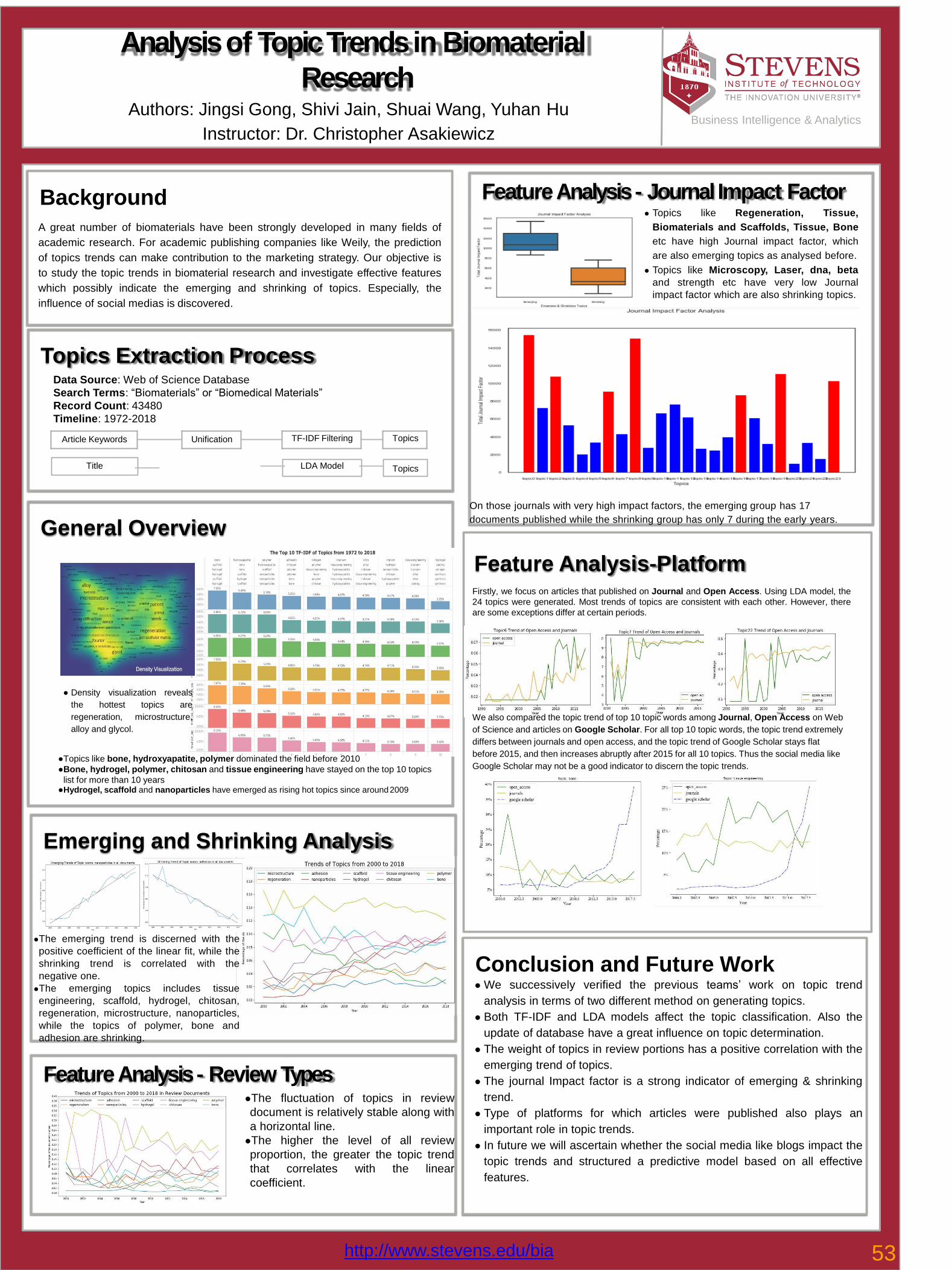
Business Intelligence & Analytics
Analysis of Topic Trends in Biomaterial
ResearchAuthors: Jingsi Gong, Shivi Jain, Shuai Wang, Yuhan Hu
Instructor: Dr. Christopher Asakiewicz
Feature Analysis - Journal Impact Factor● Topics like Regeneration, Tissue,
Biomaterials and Scaffolds, Tissue, Bone
etc have high Journal impact factor, which
are also emerging topics as analysed before.
● Topics like Microscopy, Laser, dna, beta
and strength etc have very low Journal
impact factor which are also shrinking topics.
On those journals with very high impact factors, the emerging group has 17
documents published while the shrinking group has only 7 during the early years.
General Overview
Title LDA Model Topics
Topics Extraction ProcessData Source: Web of Science Database
Search Terms: “Biomaterials” or “Biomedical Materials”
Record Count: 43480
Timeline: 1972-2018
Article Keywords Unification TF-IDF Filtering Topics
● Density visualization reveals
the hottest topics are
regeneration, microstructure,
alloy and glycol.
Background
A great number of biomaterials have been strongly developed in many fields of
academic research. For academic publishing companies like Weily, the prediction
of topics trends can make contribution to the marketing strategy. Our objective is
to study the topic trends in biomaterial research and investigate effective features
which possibly indicate the emerging and shrinking of topics. Especially, the
influence of social medias is discovered.
●Topics like bone, hydroxyapatite, polymer dominated the field before 2010
●Bone, hydrogel, polymer, chitosan and tissue engineering have stayed on the top 10 topics
list for more than 10 years●Hydrogel, scaffold and nanoparticles have emerged as rising hot topics since around2009
Emerging and Shrinking Analysis
●The emerging trend is discerned with the
positive coefficient of the linear fit, while the
shrinking trend is correlated with the
negative one.
●The emerging topics includes tissue
engineering, scaffold, hydrogel, chitosan,
regeneration, microstructure, nanoparticles,
while the topics of polymer, bone and
adhesion are shrinking.
Feature Analysis-PlatformFirstly, we focus on articles that published on Journal and Open Access. Using LDA model, the
24 topics were generated. Most trends of topics are consistent with each other. However, there
are some exceptions differ at certain periods.
We also compared the topic trend of top 10 topic words among Journal, Open Access on Web
of Science and articles on Google Scholar. For all top 10 topic words, the topic trend extremely
differs between journals and open access, and the topic trend of Google Scholar stays flat
before 2015, and then increases abruptly after 2015 for all 10 topics. Thus the social media like
Google Scholar may not be a good indicator to discern the topic trends.
Feature Analysis - Review Types●The fluctuation of topics in review
document is relatively stable along with
a horizontal line.
●The higher the level of all review
proportion, the greater the topic trend
that correlates with the linear
coefficient.
http://www.stevens.edu/bia 53
Conclusion and Future Work● We successively verified the previous teams’ work on topic trend
analysis in terms of two different method on generating topics.
● Both TF-IDF and LDA models affect the topic classification. Also the
update of database have a great influence on topic determination.
● The weight of topics in review portions has a positive correlation with the
emerging trend of topics.
● The journal Impact factor is a strong indicator of emerging & shrinking
trend.
● Type of platforms for which articles were published also plays an
important role in topic trends.
● In future we will ascertain whether the social media like blogs impact the
topic trends and structured a predictive model based on all effective
features.
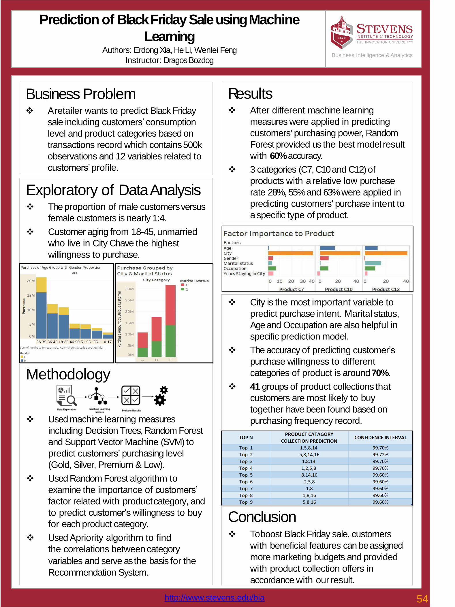
Prediction of Black Friday Sale using Machine
LearningAuthors: Erdong Xia, He Li, Wenlei Feng
Instructor: DragosBozdog
Results❖ After different machine learning
measures were applied in predicting
customers' purchasing power, Random
Forest provided us the best model result
with 60%accuracy.
❖ 3 categories (C7, C10 and C12) of
products with a relative low purchase
rate 28%, 55% and 63% were applied in
predicting customers' purchase intent to
a specific type of product.
Business Problem❖ A retailer wants to predict Black Friday
sale including customers’ consumption
level and product categories based on
transactions record which contains500k
observations and 12 variables related to
customers’ profile.
Business Intelligence & Analytics
❖ City is the most important variable to
predict purchase intent. Marital status,
Age and Occupation are also helpful in
specific prediction model.
❖ The accuracy of predicting customer’s
purchase willingness to different
categories of product is around70%.
❖ 41 groups of product collections that
customers are most likely to buy
together have been found based on
purchasing frequency record.
Conclusion❖ To boost Black Friday sale, customers
with beneficial features can beassigned
more marketing budgets and provided
with product collection offers in
accordance with our result.
Exploratory of DataAnalysis❖ The proportion of male customersversus
female customers is nearly 1:4.
❖ Customer aging from 18-45,unmarried
who live in City C have the highest
willingness to purchase.
Methodology
Model Deployment
❖ Used machine learning measures
including Decision Trees, Random Forest
and Support Vector Machine (SVM) to
predict customers’ purchasing level
(Gold, Silver, Premium & Low).
❖ Used Random Forest algorithm to
examine the importance of customers’
factor related with productcategory, and
to predict customer’s willingness to buy
for each product category.
❖ Used Apriority algorithm to find
the correlations betweencategory
variables and serve as the basis for the
Recommendation System.
http://www.stevens.edu/bia 54
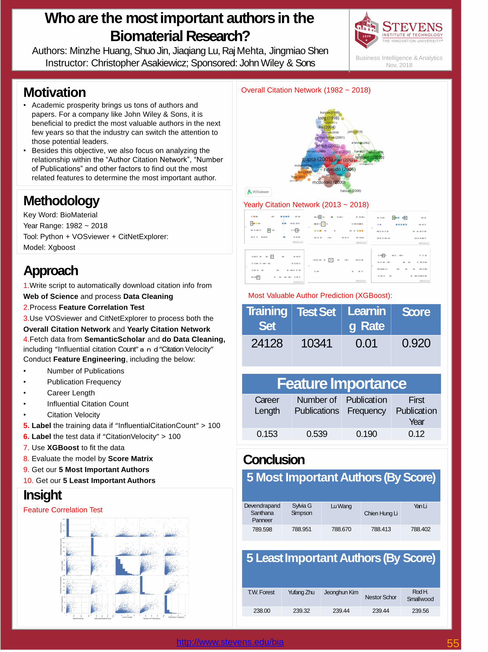
Who are the most important authors in the
Biomaterial Research?Authors: Minzhe Huang, Shuo Jin, Jiaqiang Lu, Raj Mehta, Jingmiao Shen
Instructor: Christopher Asakiewicz; Sponsored: John Wiley & Sons
Motivation• Academic prosperity brings us tons of authors and
papers. For a company like John Wiley & Sons, it is
beneficial to predict the most valuable authors in the next
few years so that the industry can switch the attention to
those potential leaders.
• Besides this objective, we also focus on analyzing the
relationship within the “Author Citation Network”, “Number
of Publications” and other factors to find out the most
related features to determine the most important author.
Business Intelligence & Analytics
Nov, 2018
MethodologyKey Word: BioMaterial
Year Range: 1982 ~ 2018
Tool: Python + VOSviewer + CitNetExplorer:
Model: Xgboost
Approach1.Write script to automatically download citation info from
Web of Science and process Data Cleaning
2.Process Feature Correlation Test
3.Use VOSviewer and CitNetExplorer to process both the
Overall Citation Network and Yearly Citation Network
4.Fetch data from SemanticScholar and do Data Cleaning,
including “Influential citation Count”and“Citation Velocity”
Conduct Feature Engineering, including the below:
• Number of Publications
• Publication Frequency
• Career Length
• Influential Citation Count
• Citation Velocity
5. Label the training data if “InfluentialCitationCount” > 100
6. Label the test data if “CitationVelocity” > 100
7. Use XGBoost to fit the data
8. Evaluate the model by Score Matrix
9. Get our 5 Most Important Authors
10. Get our 5 Least Important Authors
InsightFeature Correlation Test
Most Valuable Author Prediction (XGBoost):
Yearly Citation Network (2013 ~ 2018)
Overall Citation Network (1982 ~ 2018)
TestSet ScoreTraining
Set
24128 10341
Learnin
g Rate
0.01 0.920
Feature ImportanceCareer Number of Publication
Length Publications Frequency
0.153 0.539 0.190
First
Publication
Year
0.12
Conclusion
5 Most Important Authors (By Score)
Sylvia G
SimpsonLuWang
Chien Hung Li
YanLiDevendrapand
Santhana
Panneer
789.598 788.951 788.670 788.413 788.402
5 Least Important Authors (By Score)
T. W.Forest Yufang Zhu Jeonghun KimNestor Schor
238.00 239.32 239.44 239.44
Rod H.
Smallwood
239.56
http://www.stevens.edu/bia 55
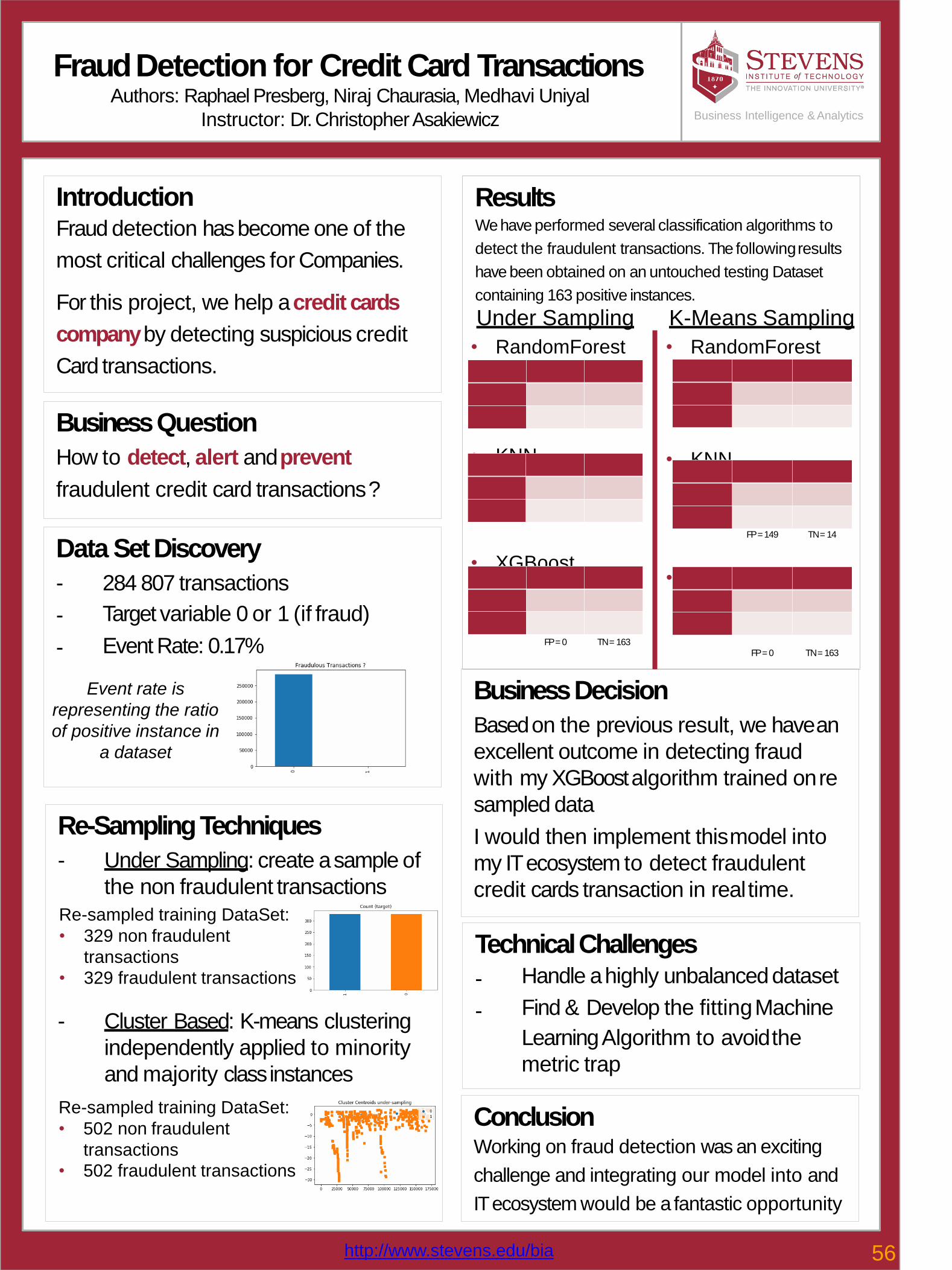
Fraud Detection for Credit Card TransactionsAuthors: Raphael Presberg, Niraj Chaurasia, Medhavi Uniyal
Instructor: Dr. ChristopherAsakiewicz
IntroductionFraud detection has become one of the
most critical challenges for Companies.
For this project, we help a credit cards
company by detecting suspicious credit
Card transactions.
BusinessQuestion
How to detect, alert andprevent
fraudulent credit card transactions?
ConclusionWorking on fraud detection was an exciting
challenge and integrating our model into and
IT ecosystem would be a fantastic opportunity
Business Intelligence & Analytics
BusinessDecision
Based on the previous result, we havean
excellent outcome in detecting fraud
with my XGBoost algorithm trained onre
sampled data
I would then implement thismodel into
my IT ecosystem to detect fraudulent
credit cards transaction in realtime.
Data SetDiscovery
-
-
-
284 807 transactions
Target variable 0 or 1 (if fraud)
Event Rate: 0.17%
Re-SamplingTechniques
- Under Sampling: create a sample of
the non fraudulent transactions
- Cluster Based: K-means clustering
independently applied to minority
and majority classinstances
Re-sampled training DataSet:
• 329 non fraudulent
transactions
• 329 fraudulent transactions
Re-sampled training DataSet:
• 502 non fraudulent
transactions
• 502 fraudulent transactions
Event rate is
representing the ratio
of positive instance in
a dataset
TechnicalChallenges
-
-
Handle a highly unbalanceddataset
Find & Develop the fittingMachine
Learning Algorithm to avoidthe
metric trap
ResultsWe have performed several classification algorithms to
detect the fraudulent transactions. The followingresults
have been obtained on an untouched testing Dataset
containing 163 positive instances.
Under Sampling K-Means Sampling
• RandomForestPredicted:
Predicte
d: 1 0
Actual: TP= 93799 FN =25
1
Actual: FP= 0 TN = 163
0
• KNNPredicted: Predicted:
1 0
Actual: TP=57469 FN =36355
1
Actual: FP=56 TN = 107
0
• XGBoostPredicted:
Predicte
d: 1 0
Actual: TP= 93824 FN =0
1
Actual: FP= 0 TN = 163
0
• RandomForestPredicted:
Predicte
d: 1 0
Actual: TP=18265 FN =75568
1
Actual: FP= 0 TN = 163
0
• KNNPredicted:
Predicte
d: 1 0
Actual: TP=93823 FN =1
1
Actual: FP=149 TN = 14
0
• XGBoostPredicted:
Predicte
d: 1 0
Actual: TP=77299 FN =16525
1
Actual: FP= 0 TN = 163
0
http://www.stevens.edu/bia 56
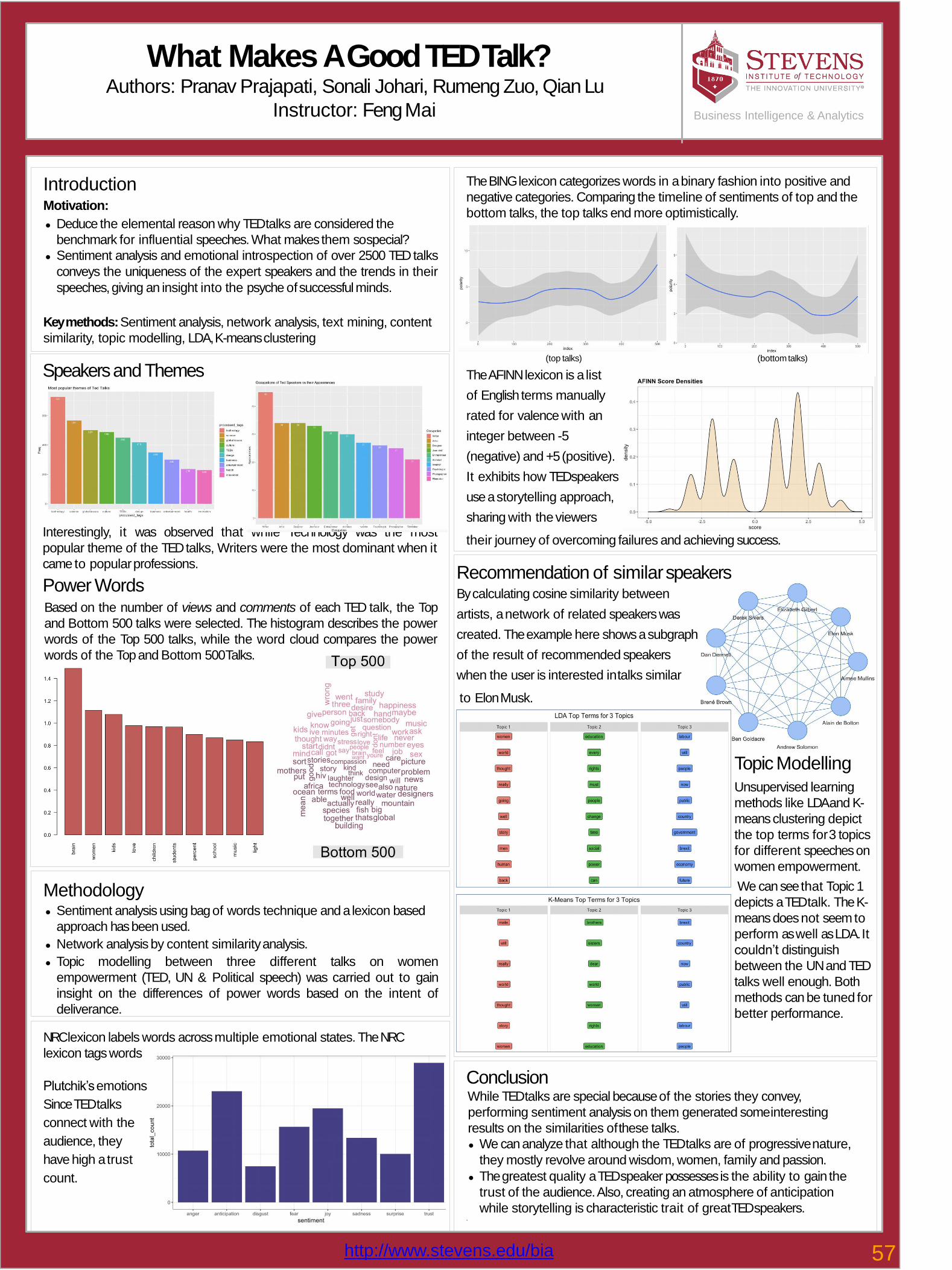
What Makes A Good TEDTalk?Authors: Pranav Prajapati, Sonali Johari, Rumeng Zuo, Qian Lu
Instructor: FengMai
The BING lexicon categorizes words in a binary fashion into positive and
negative categories. Comparing the timeline of sentiments of top and the
bottom talks, the top talks end more optimistically.
(top talks) (bottomtalks)
The AFINN lexicon is a list
of English terms manually
rated for valence with an
integer between -5
(negative) and +5(positive).
It exhibits how TEDspeakers
use a storytelling approach,
sharing with theviewers
their journey of overcoming failures and achieving success.
IntroductionMotivation:
● Deduce the elemental reason why TED talks are considered the
benchmark for influential speeches. What makes them sospecial?
● Sentiment analysis and emotional introspection of over 2500 TEDtalks
conveys the uniqueness of the expert speakers and the trends in their
speeches,giving an insight into the psyche ofsuccessfulminds.
Key methods: Sentiment analysis, network analysis, text mining, content
similarity, topic modelling, LDA, K-meansclustering
Speakers and Themes
Interestingly, it was observed that while Technology was the most
popular theme of the TEDtalks, Writers were the most dominant when it
came to popularprofessions.
Power WordsBased on the number of views and comments of each TED talk, the Top
and Bottom 500 talks were selected. The histogram describes the power
words of the Top 500 talks, while the word cloud compares the power
words of the Topand Bottom 500Talks.
ConclusionWhile TED talks are special because of the stories they convey,
performing sentiment analysis on them generated someinteresting
results on the similarities ofthese talks.
● We can analyze that although the TED talks are of progressivenature,
they mostly revolve around wisdom, women, family and passion.
● The greatest quality a TED speaker possesses is the ability to gain the
trust of the audience.Also, creating an atmosphere of anticipation
while storytelling is characteristic trait of greatTED speakers.`
Business Intelligence & Analytics
Methodology● Sentiment analysis using bag of words technique and a lexicon based
approach has been used.
● Network analysis by content similarityanalysis.
● Topic modelling between three different talks on women
empowerment (TED, UN & Political speech) was carried out to gain
insight on the differences of power words based on the intent of
deliverance.
NRC lexicon labels words across multiple emotional states. The NRC
lexicon tagswords
according to the8
Plutchik’semotions
Since TED talks
connect with the
audience, they
have high a trust
count.
Recommendation of similarspeakersBy calculating cosine similarity between
artists, a network of related speakers was
created. The example here shows a subgraph
of the result of recommended speakers
when the user is interested intalks similar
to ElonMusk.
Topic Modelling
Unsupervised learning
methods like LDA and K-
means clustering depict
the top terms for3 topics
for different speeches on
women empowerment.
We can see that Topic 1
depicts a TED talk. The K-
means does not seem to
perform as well as LDA. It
couldn’t distinguish
between the UN and TED
talks well enough. Both
methods can be tuned for
better performance.
http://www.stevens.edu/bia 57

Optimizing London Fire Station Resources to Better
Serve the CommunityAuthors: Sonali Johari, Pranav Prajapati, David McFarland, Erika Deckter and Marielle Nwana
Instructor: TedStohr
Motivation
By simulating real-world emergency scenarios, fire station resources can be
efficiently deployed to each incident while minimizing overall travel distance
for the fire engines. This analysis also showed the impact of adding
additional resources to existing fire stations in order to better serve the
community.
Data
Using data provided by the London Fire Brigade as well as informationfrom
Kaggle, we were able to obtain a historical database for over 85,000 fire
incidents for 2017 (from January toOctober).
KeyMethods
Integer Programming Optimization, Simulation, Great Circle distance andR
Simulation
• 9,600 simulated time periods (15-minute intervals over 100days)
• A zero-truncated Poisson distribution was used to determine the number of
incidents in each simulation period
• Incidents for each time period were selected using a random draw of a
subset of the historicaldata
• The Integer Programming (IP) optimization model was applied to each
simulation period
• The model assumed fire engines are deployed at the end of each 15-
minute period and do not return for 30 minutes (i.e., a fire engine deployed
in the previous two simulation periods cannot be used in the current
period
Incidents Per 15-Minute Period for Historical Data and Simulation Set
Business Intelligence & Analytics
Concentration of Simulated Incidents Over 100
Days and Fire Stations Included in Analysis
Perio
d
ID
Inciden
t
Numbe
r
Incident Fire Engine Deployment
Dowgate Euston Holloway Islington
Kentish
Town Paddingto
n
Soho
West
Hampstead
26 071065-03062017 0 0 1 0 0 0 0 0
26 111710-18082017 0 0 0 0 0 0 0 1
26 079544-18062017 0 0 0 0 0 1 0 0
26 141792-21102017 0 0 0 0 0 0 1 0
27 061388-16052017 0 1 0 0 0 0 0 0
27 024617-27022017 0 0 0 0 0 0 1 0
27 116856-29082017 0 0 0 0 1 0 0 0
28 026377-03032017 0 0 0 0 0 1 0 0
28 070188-02062017 1 0 0 0 0 0 0 0
28 039442-02042017 0 0 0 1 0 0 0 0
29 082627-23062017 0 0 0 0 1 0 0 0
29 142806-23102017 0 0 1 0 0 0 0 0
30 026696-04032017 0 0 0 0 1 0 0 0
SensitivityAnalysisFire Engine Availability
Dowgate Euston Holloway Islington
Kentish
Town Paddingto
n
Soho
West
Hampstead
Total Fire
Engines
BaseModel 1 1 1 1 2 2 2 2 12
Sensitivity +1 2 2 2 2 3 3 3 3 20
Sensitivity +2 3 3 3 3 4 4 4 4 28• The base analysis was performed using actual fire engine counts from London Fire
Brigade’s fleet list (as of September 2017).• Two sensitivity analyses were performed by adding 1 fire engine and 2 fire engines to the
starting fleet of each fire station.
• For the base analysis, slightly over 400 simulation periods (about 4.4%) did not have a
sufficient number of fire engines available to deploy to all incidents for that time period
(i.e., there was no feasible solution for the optimization problem).
• When increasing the starting number of fire engines at each station by 1, there was only
one simulation without a feasible solution.
• The sensitivity analysis with two additional fire engines per station had no infeasible
solutions.
Optimization ModelInputs
Distance Matrix, D
𝑑𝑖𝑗= distance between ith incident and jth fire station
Delay Factor Matrix, F
𝑓𝑖𝑗= randomly generated factor (between 0 and 1) to simulate arrival delays
Effective Distance Matrix, E
𝑒𝑖𝑗= 𝑑𝑖𝑗+ 𝑓𝑖𝑗𝑑𝑖𝑓= (1 + 𝑓𝑖𝑗)𝑑𝑖𝑓
Availability Vector,A
𝑎𝑗= number of fire engines available at jth station
Decision Variable
Sent Matrix, S1,
𝑠𝑖𝑗= 0,iffireengineisdispatchedtoincidentifromstationj iffireengineis
notsenttoincidentifromstaionj
Constraints
𝑖𝑠𝑖𝑗= 1, one fire engine is dispatched to eachincident
𝑗𝑠𝑖𝑗≤𝑎𝑗, the total number of fire engines dispatched from a station cannot exceed the
available number
Output
Minimize the Total EffectiveDistance
𝑠𝑖𝑗𝑒𝑖𝑗𝑖 𝑗
ResultsSample Result Output for Select Simulation Periods
Simulated Incidents
by Fire Station
2000
Borough shapefile
contains National
Statistics and Ordnance
Survey data
© Crown copyright and
database right 2018
3000
http://www.stevens.edu/bia 58
5000
Count of
Simulated
Incidents
Perio
d
ID
Total Fire EngineDeployment
Total
Incident
s
Total
Effectiv
e
Distanc
e
Dowgate Euston Holloway Islington
Kentish
Town Paddingto
n
Soho
West
Hampstead
26 0 0 1 0 0 1 1 1 4 11.43
27 0 1 0 0 1 0 1 0 3 32.46
28 1 0 0 1 0 1 0 0 3 11.23
29 0 0 1 0 1 0 0 0 2 18.08
30 0 0 0 0 1 0 0 0 1 0.41
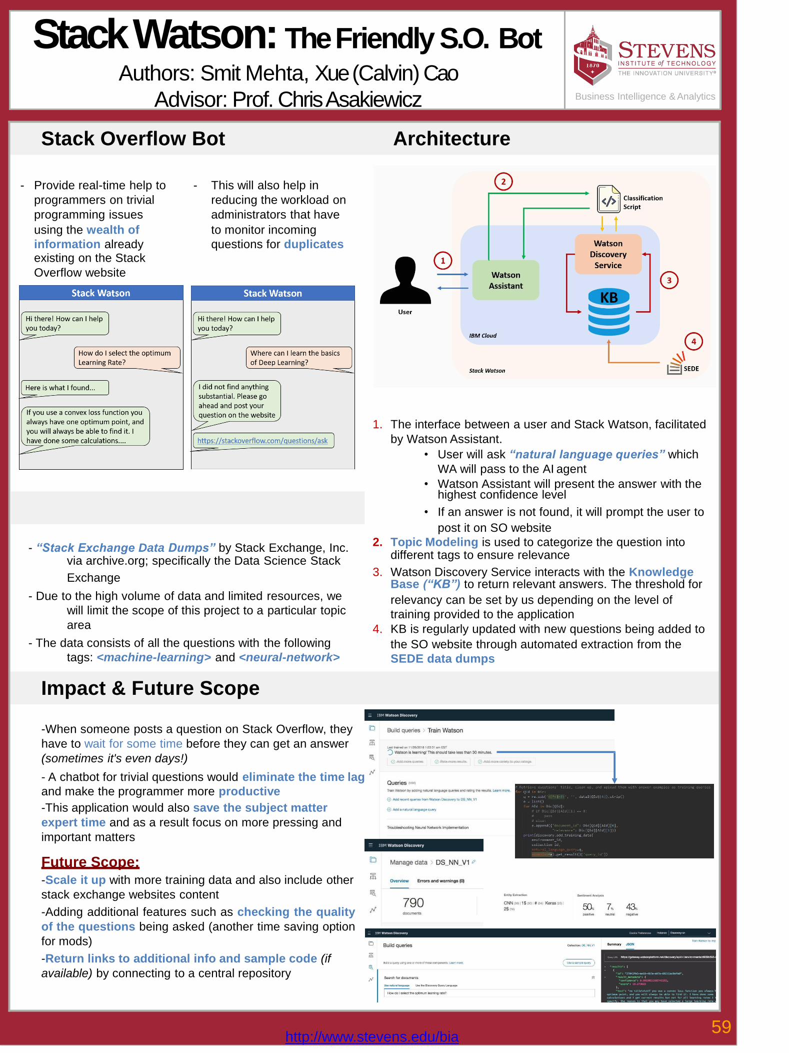
Stack Watson: The Friendly S.O. BotAuthors: Smit Mehta, Xue (Calvin) Cao
Advisor: Prof. ChrisAsakiewicz Business Intelligence & Analytics
Stack Overflow Bot Architecture
- Provide real-time help to - This will also help in
programmers on trivial reducing the workload on
programming issues administrators that have
using the wealth of to monitor incoming
information already questions for duplicatesexisting on the Stack
Overflow website
1. The interface between a user and Stack Watson, facilitated
by Watson Assistant.
• User will ask “natural language queries” which
WA will pass to the AI agent
• Watson Assistant will present the answer with thehighest confidence level
Data & Scope • If an answer is not found, it will prompt the user to
post it on SO website
- “Stack Exchange Data Dumps” by Stack Exchange, Inc.2. Topic Modeling is used to categorize the question into
via archive.org; specifically the Data Science Stackdifferent tags to ensure relevance
Exchange3. Watson Discovery Service interacts with the Knowledge
Base (“KB”) to return relevant answers. The threshold for- Due to the high volume of data and limited resources, we relevancy can be set by us depending on the level of
will limit the scope of this project to a particular topic training provided to the applicationarea 4. KB is regularly updated with new questions being added to
- The data consists of all the questions with the following the SO website through automated extraction from thetags: <machine-learning> and <neural-network> SEDE data dumps
Impact & Future Scope
-When someone posts a question on Stack Overflow, they
have to wait for some time before they can get an answer
(sometimes it's even days!)
- A chatbot for trivial questions would eliminate the time lag
and make the programmer more productive
-This application would also save the subject matter
expert time and as a result focus on more pressing and
important matters
Future Scope:-Scale it up with more training data and also include other
stack exchange websites content
-Adding additional features such as checking the quality
of the questions being asked (another time saving option
for mods)
-Return links to additional info and sample code (if
available) by connecting to a central repository
http://www.stevens.edu/bia59
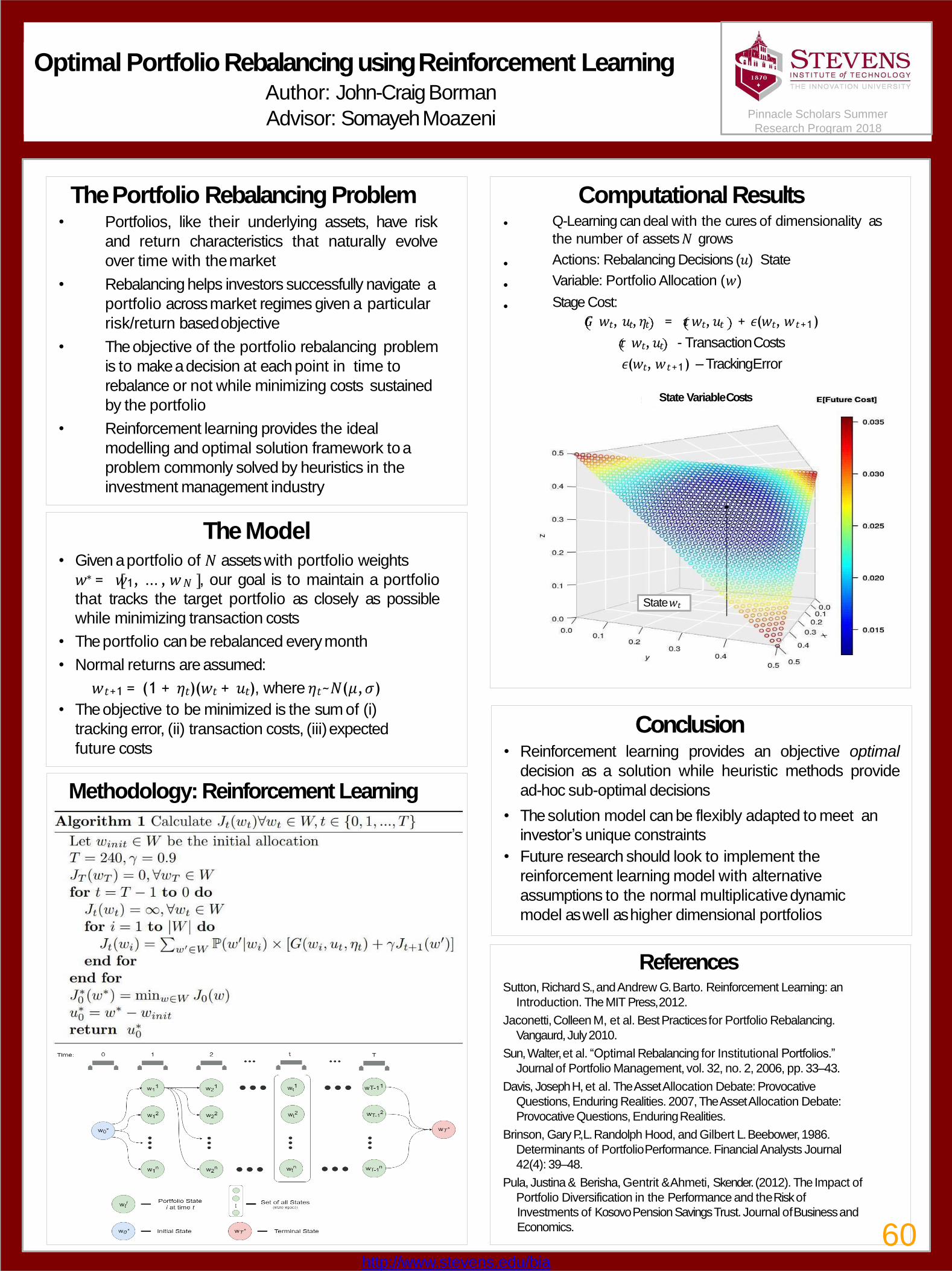
Optimal Portfolio Rebalancing using Reinforcement LearningAuthor: John-CraigBorman
Advisor: SomayehMoazeni
The Portfolio Rebalancing Problem• Portfolios, like their underlying assets, have risk
and return characteristics that naturally evolve
over time with themarket
• Rebalancing helps investors successfully navigate a
portfolio across market regimes given a particular
risk/return basedobjective
• The objective of the portfolio rebalancing problem
is to make a decision at each point in time to
rebalance or not while minimizing costs sustained
by the portfolio
• Reinforcement learning provides the ideal
modelling and optimal solution framework toa
problem commonly solved by heuristics in the
investment management industry
•
•
•
•
Computational ResultsQ-Learning can deal with the cures of dimensionality as
the number of assets 𝑁 grows
Actions: Rebalancing Decisions (𝑢) State
Variable: Portfolio Allocation (𝑤)
Stage Cost:
𝐺 𝑤𝑡, 𝑢𝑡,𝜂𝑡 = 𝜏𝑤𝑡,𝑢𝑡 + 𝜖(𝑤𝑡, 𝑤𝑡+1)
𝜏 𝑤𝑡,𝑢𝑡 - TransactionCosts
𝜖(𝑤𝑡, 𝑤𝑡+1) – TrackingError
The Model• Given a portfolio of 𝑁 assets with portfolio weights
𝑤∗ = 𝑤1, … ,𝑤𝑁 , our goal is to maintain a portfolio
that tracks the target portfolio as closely as possible
while minimizing transaction costs
• The portfolio can be rebalanced everymonth
• Normal returns are assumed:
𝑤𝑡+1 = (1 + 𝜂𝑡)(𝑤𝑡 + 𝑢𝑡), where 𝜂𝑡~𝑁(𝜇,𝜎)
• The objective to be minimized is the sum of (i)
tracking error, (ii) transaction costs, (iii)expected
future costs
Conclusion• Reinforcement learning provides an objective optimal
decision as a solution while heuristic methods provide
ad-hoc sub-optimal decisions
• The solution model can be flexibly adapted to meet an
investor’s unique constraints
• Future research should look to implement the
reinforcement learning model with alternative
assumptions to the normal multiplicativedynamic
model as well as higher dimensional portfolios
Pinnacle Scholars Summer
Research Program 2018
Methodology: Reinforcement Learning
State𝑤𝑡
State VariableCosts
ReferencesSutton, Richard S., and Andrew G. Barto. Reinforcement Learning: an
Introduction. The MIT Press,2012.
Jaconetti,Colleen M, et al. Best Practicesfor Portfolio Rebalancing.
Vangaurd, July2010.
Sun,Walter,et al. “Optimal Rebalancing for Institutional Portfolios.”
Journal of Portfolio Management, vol. 32, no. 2, 2006, pp. 33–43.
Davis, Joseph H, et al. The Asset Allocation Debate: Provocative
Questions, Enduring Realities. 2007, The Asset Allocation Debate:
Provocative Questions, EnduringRealities.
Brinson, Gary P., L. Randolph Hood, and Gilbert L. Beebower,1986.
Determinants of PortfolioPerformance. Financial Analysts Journal
42(4): 39–48.
Pula, Justina & Berisha, Gentrit &Ahmeti, Skender. (2012). The Impact of
Portfolio Diversification in the Performance and theRisk of
Investments of Kosovo Pension Savings Trust. Journal ofBusiness and
Economics.
http://www.stevens.edu/bia
60
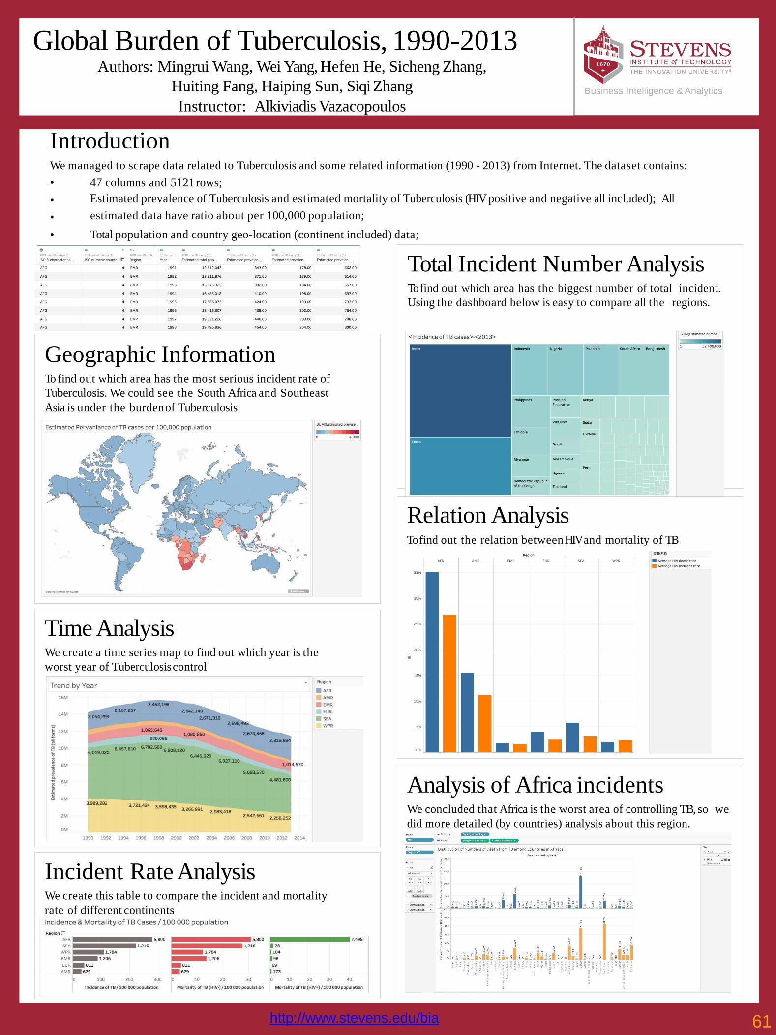
Global Burden of Tuberculosis, 1990-2013Authors: Mingrui Wang, Wei Yang, Hefen He, Sicheng Zhang,
Huiting Fang, Haiping Sun, Siqi Zhang
Instructor: Alkiviadis Vazacopoulos
IntroductionWe managed to scrape data related to Tuberculosis and some related information (1990 - 2013) from Internet. The dataset contains:
•
•
•
•
47 columns and 5121rows;
Estimated prevalence of Tuberculosis and estimated mortality of Tuberculosis (HIV positive and negative all included); All
estimated data have ratio about per 100,000 population;
Total population and country geo-location (continent included) data;
Geographic InformationTo find out which area has the most serious incident rate of
Tuberculosis. We could see the South Africa and Southeast
Asia is under the burdenof Tuberculosis
Business Intelligence & Analytics
http://www.stevens.edu/bia
Time AnalysisWe create a time series map to find out which year is the
worst year of Tuberculosiscontrol
Incident Rate AnalysisWe create this table to compare the incident and mortality
rate of different continents
Total Incident Number AnalysisTo find out which area has the biggest number of total incident.
Using the dashboard below is easy to compare all the regions.
Relation AnalysisTo find out the relation betweenHIV and mortality of TB
Analysis of Africa incidentsWe concluded that Africa is the worst area of controlling TB, so we
did more detailed (by countries) analysis about this region.
61
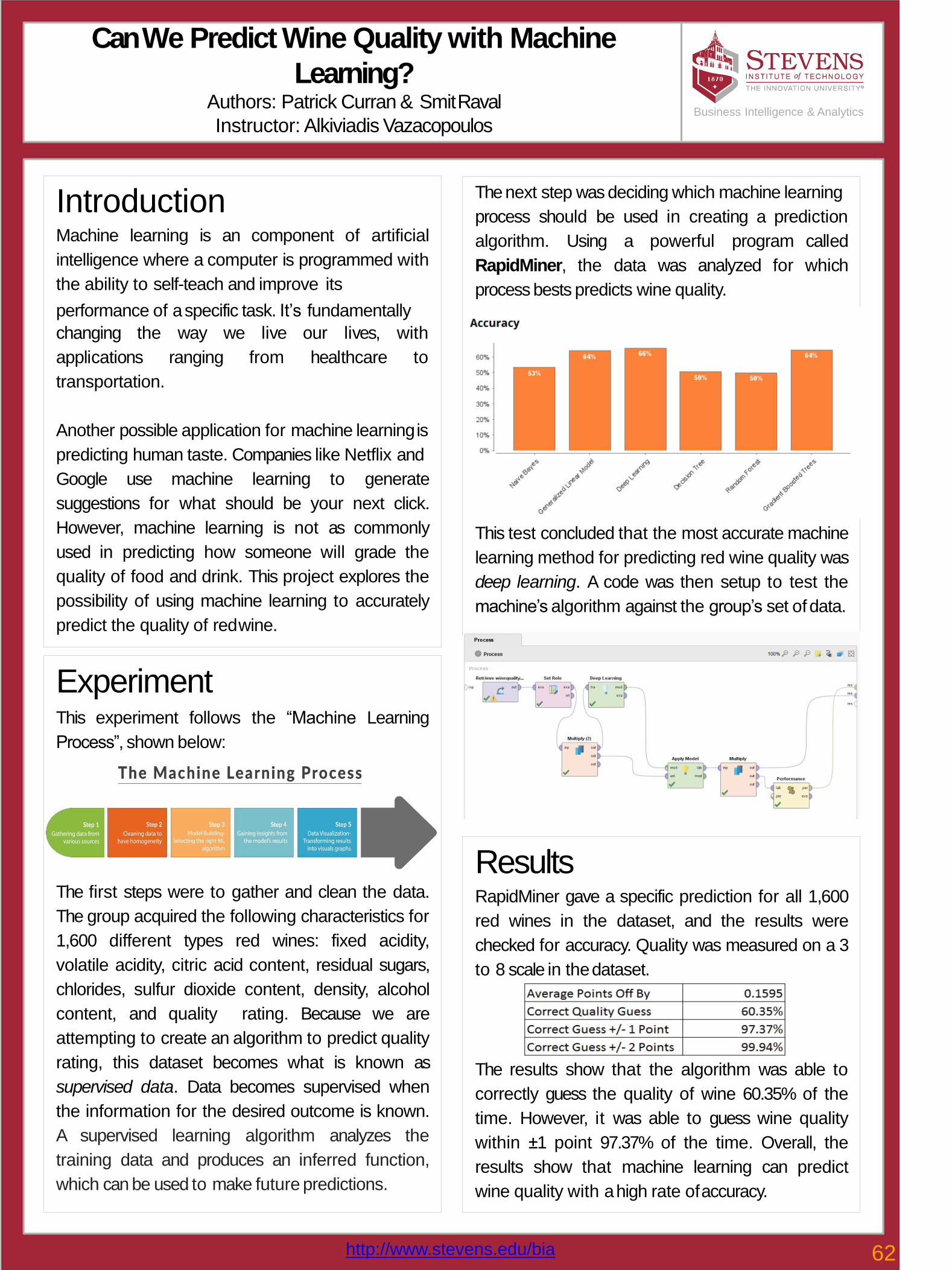
Can We Predict Wine Quality with Machine
Learning?Authors: Patrick Curran & SmitRaval
Instructor: Alkiviadis Vazacopoulos
The next step was deciding which machine learning
process should be used in creating a prediction
called
which
algorithm. Using a powerful program
RapidMiner, the data was analyzed for
process bests predicts wine quality.
This test concluded that the most accurate machine
learning method for predicting red wine quality was
deep learning. A code was then setup to test the
machine’s algorithm against the group’s set ofdata.
IntroductionMachine learning is an component of artificial
intelligence where a computer is programmed with
the ability to self-teach and improve its
performance of a specific task. It’s fundamentally
we live our lives, with
from healthcare to
changing the way
applications ranging
transportation.
Another possible application for machine learningis
predicting human taste. Companies like Netflix and
Google use machine learning to generate
suggestions for what should be your next click.
However, machine learning is not as commonly
used in predicting how someone will grade the
quality of food and drink. This project explores the
possibility of using machine learning to accurately
predict the quality of redwine.
Business Intelligence & Analytics
ExperimentThis experiment follows the “Machine Learning
Process”, shown below:
The first steps were to gather and clean the data.
The group acquired the following characteristics for
1,600 different types red wines: fixed acidity,
volatile acidity, citric acid content, residual sugars,
chlorides, sulfur dioxide content, density, alcohol
content, and quality rating. Because we are
attempting to create an algorithm to predict quality
rating, this dataset becomes what is known as
supervised data. Data becomes supervised when
the information for the desired outcome is known.
A supervised learning algorithm analyzes the
training data and produces an inferred function,
which can be used to make future predictions.
ResultsRapidMiner gave a specific prediction for all 1,600
red wines in the dataset, and the results were
checked for accuracy. Quality was measured on a 3
to 8 scale in thedataset.
The results show that the algorithm was able to
correctly guess the quality of wine 60.35% of the
time. However, it was able to guess wine quality
within ±1 point 97.37% of the time. Overall, the
results show that machine learning can predict
wine quality with ahigh rate ofaccuracy.
http://www.stevens.edu/bia 62
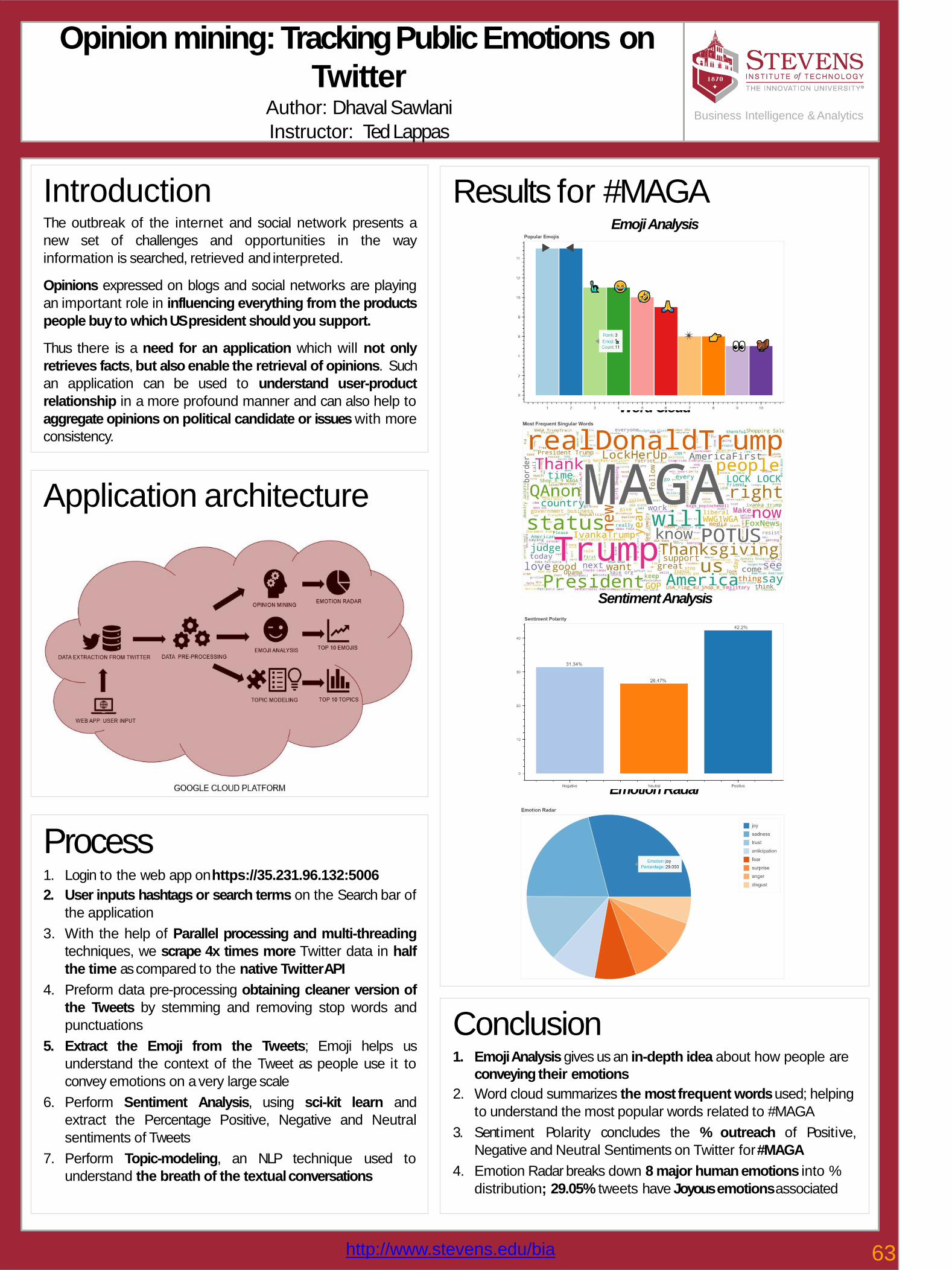
Opinion mining: Tracking Public Emotions on
TwitterAuthor: Dhaval Sawlani
Instructor: TedLappas
Results for #MAGAEmojiAnalysis
Word Cloud
SentimentAnalysis
EmotionRadar
Business Intelligence & Analytics
Application architecture
IntroductionThe outbreak of the internet and social network presents a
new set of challenges and opportunities in the way
information is searched, retrieved and interpreted.
Opinions expressed on blogs and social networks are playing
an important role in influencing everything from the products
people buyto whichUSpresident shouldyou support.
Thus there is a need for an application which will not only
retrieves facts, but also enable the retrieval of opinions. Such
an application can be used to understand user-product
relationship in a more profound manner and can also help to
aggregate opinions on political candidate or issues with more
consistency.
Process1. Login to the web app onhttps://35.231.96.132:5006
2. User inputs hashtags or search terms on the Search bar of
the application
3. With the help of Parallel processing and multi-threading
techniques, we scrape 4x times more Twitter data in half
the time ascompared to the native TwitterAPI
4. Preform data pre-processing obtaining cleaner version of
the Tweets by stemming and removing stop words and
punctuations
5. Extract the Emoji from the Tweets; Emoji helps us
understand the context of the Tweet as people use it to
convey emotions on avery large scale
6. Perform Sentiment Analysis, using sci-kit learn and
extract the Percentage Positive, Negative and Neutral
sentiments of Tweets
7. Perform Topic-modeling, an NLP technique used to
understand the breath of the textualconversations
Conclusion1. Emoji Analysis gives us an in-depth idea about how people are
conveying their emotions
2. Word cloud summarizes the most frequent words used; helping
to understand the most popular words related to #MAGA
3. Sentiment Polarity concludes the % outreach of Positive,
Negative and Neutral Sentiments on Twitter for#MAGA
4. Emotion Radar breaks down 8 major human emotions into %
distribution; 29.05% tweets have Joyous emotionsassociated
http://www.stevens.edu/bia 63
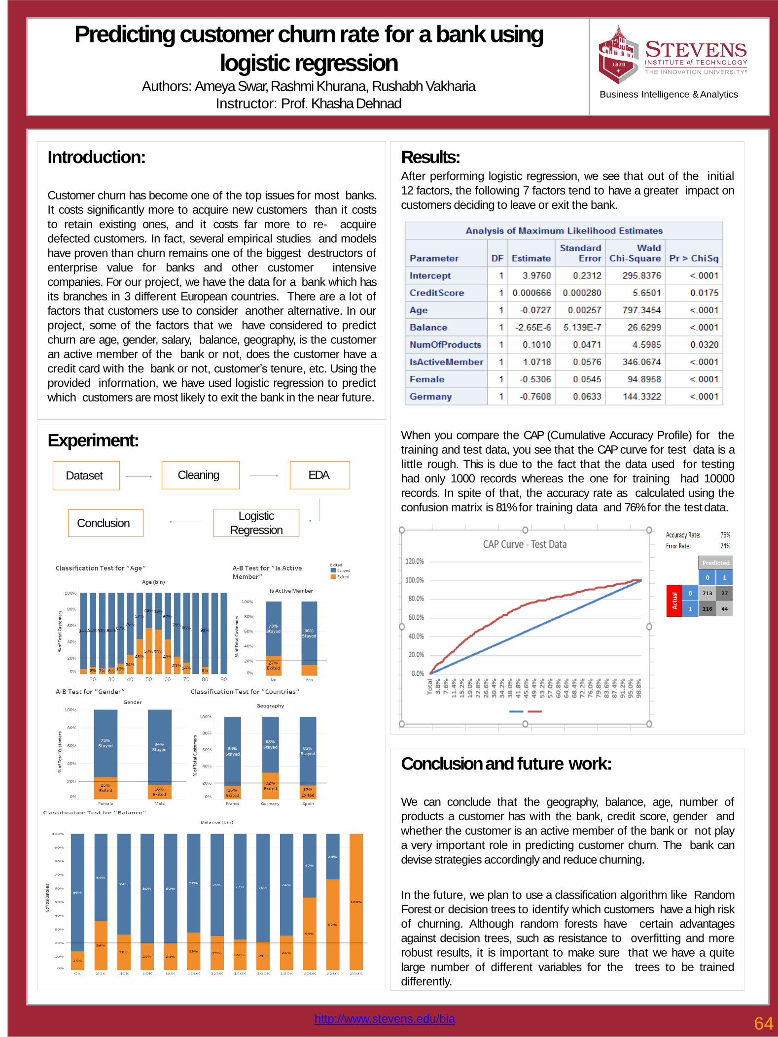
Predicting customer churn rate for a bank using
logistic regressionAuthors: Ameya Swar, Rashmi Khurana, Rushabh Vakharia
Instructor: Prof. KhashaDehnad
Results:After performing logistic regression, we see that out of the initial
12 factors, the following 7 factors tend to have a greater impact on
customers deciding to leave or exit the bank.
When you compare the CAP (Cumulative Accuracy Profile) for the
training and test data, you see that the CAP curve for test data is a
little rough. This is due to the fact that the data used for testing
had only 1000 records whereas the one for training had 10000
records. In spite of that, the accuracy rate as calculated using the
confusion matrix is 81%for training data and 76%for the test data.
Introduction:
Customer churn has become one of the top issues for most banks.
It costs significantly more to acquire new customers than it costs
to retain existing ones, and it costs far more to re- acquire
defected customers. In fact, several empirical studies and models
have proven than churn remains one of the biggest destructors of
enterprise value for banks and other customer intensive
companies. For our project, we have the data for a bank which has
its branches in 3 different European countries. There are a lot of
factors that customers use to consider another alternative. In our
project, some of the factors that we have considered to predict
churn are age, gender, salary, balance, geography, is the customer
an active member of the bank or not, does the customer have a
credit card with the bank or not, customer’s tenure, etc. Using the
provided information, we have used logistic regression to predict
which customers are most likely to exit the bank in the near future.
Experiment:
Conclusion and future work:
We can conclude that the geography, balance, age, number of
products a customer has with the bank, credit score, gender and
whether the customer is an active member of the bank or not play
a very important role in predicting customer churn. The bank can
devise strategies accordingly and reduce churning.
In the future, we plan to use a classification algorithm like Random
Forest or decision trees to identify which customers have a high risk
of churning. Although random forests have certain advantages
against decision trees, such as resistance to overfitting and more
robust results, it is important to make sure that we have a quite
large number of different variables for the trees to be trained
differently.
Business Intelligence & Analytics
http://www.stevens.edu/bia
Dataset Cleaning EDA
Logistic
RegressionConclusion
64
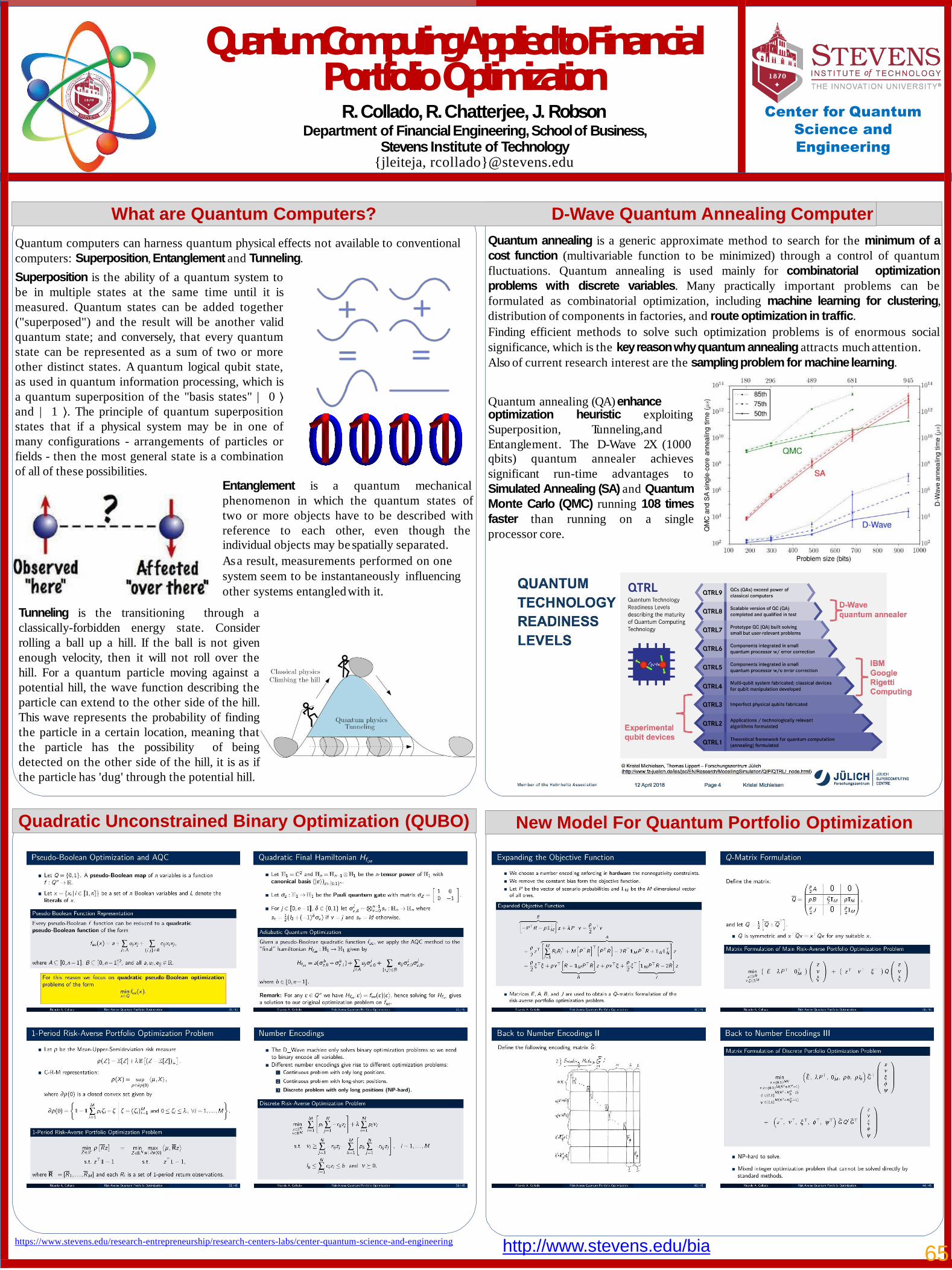
Quantum Computing Applied to Financial PortfolioOptimization
R. Collado, R. Chatterjee, J. RobsonDepartment of Financial Engineering, School of Business,
Stevens Institute of Technology{jleiteja, rcollado}@stevens.edu
Center for Quantum
Science and
Engineering
Quadratic Unconstrained Binary Optimization (QUBO)
What are Quantum Computers? D-Wave Quantum Annealing Computer
New Model For Quantum Portfolio Optimization
https://www.stevens.edu/research-entrepreneurship/research-centers-labs/center-quantum-science-and-engineering
Quantum computers can harness quantum physical effects not available to conventional
computers: Superposition, Entanglement and Tunneling.
Superposition is the ability of a quantum system to
be in multiple states at the same time until it is
measured. Quantum states can be added together
("superposed") and the result will be another valid
quantum state; and conversely, that every quantum
state can be represented as a sum of two or more
other distinct states. A quantum logical qubit state,
as used in quantum information processing, which is
a quantum superposition of the "basis states" | 0 ⟩and | 1 ⟩. The principle of quantum superposition
states that if a physical system may be in one of
many configurations - arrangements of particles or
fields - then the most general state is a combination
of all of these possibilities.
Entanglement is a quantum mechanical
phenomenon in which the quantum states of
two or more objects have to be described with
reference to each other, even though the
individual objects may be spatially separated.
As a result, measurements performed on one
system seem to be instantaneously influencing
other systems entangledwith it.
Tunneling is the transitioning through a
classically-forbidden energy state. Consider
rolling a ball up a hill. If the ball is not given
enough velocity, then it will not roll over the
hill. For a quantum particle moving against a
potential hill, the wave function describing the
particle can extend to the other side of the hill.
This wave represents the probability of finding
the particle in a certain location, meaning that
the particle has the possibility of being
detected on the other side of the hill, it is as if
the particle has 'dug' through the potential hill.
Quantum annealing is a generic approximate method to search for the minimum of a
cost function (multivariable function to be minimized) through a control of quantum
fluctuations. Quantum annealing is used mainly for combinatorial optimization
problems with discrete variables. Many practically important problems can be
formulated as combinatorial optimization, including machine learning for clustering,
distribution of components in factories, and route optimization in traffic.
Finding efficient methods to solve such optimization problems is of enormous social
significance, which is the keyreasonwhyquantum annealing attracts much attention.
Also of current research interest are the samplingproblem for machinelearning.
Quantum annealing (QA) enhanceoptimization
Superposition,
Entanglement.
heuristic exploiting
Tunneling,and
The D-Wave 2X (1000
qbits) quantum annealer achieves
significant run-time advantages to
Simulated Annealing (SA) and Quantum
Monte Carlo (QMC) running 108 times
faster than running on a single
processor core.
http://www.stevens.edu/bia 65

Object Detection in Autonomous Driving CarAuthors: Taru Tak, Pravin Mukare, Amit Agarwal
Instructor: ChristopherAsakiewicz
INTRODUCTION
Object detection is an essential component for autonomous driving cars. Accurate detection of vehicles, street
buildings, pedestrians and road signs could assist self-driving cars the drive as safely as humans. However,
conventional classification-after-localization methods are in slow in real-time situations. We need an object
detection model which can detect object with high accuracy while also running in real-time.
MODEL
We used a specialized Convolutional Neural Network algorithm called YOLO(You only
look once). It assists in real time object prediction. Solution is implemented with
Python, TensorFlow and Keras.
YOLO requires a large dataset and is computationally very expensive to train. Hence,
weights that have been pre-trained on Microsoft’s COCO dataset have been used. MS-
COCO contains 91 labelled object types in 328Kimages.
Implementation Details:
• Our model runs a pre-processed input image through a DeepCNN.
• We filter through all the boxes using non-maxsuppression.
• Filter out detected object classes with lowprobability.
• Use Intersection over Union (IoU) to get thefinal bounding box.
• We get output image of detected objects and corresponding boundingboxes.
Business Intelligence & Analytics
OBJECTIVE
Given an image taken by a camera mounted on top of the car, our objective would be to successfully detect a car in
the image and put a bounding box around thecar.
Input: Image from Mounted Camera Output: Detected Cars withboxes
CONCLUSION
This implementation provides a practical object recognition example that will enable
autonomous applications such as self-driving cars. It allows the car to build an accurate
mapping of its surrounding which will allow it to steer safely in complex surroundings.
For now, it can be used to augment human driving capabilities. The object recognition
task can be paired with segmentation and GPS to mark lanes, pedestrian cross-walks,
etc. to develop more robustsolutions.
http://www.stevens.edu/bia 66
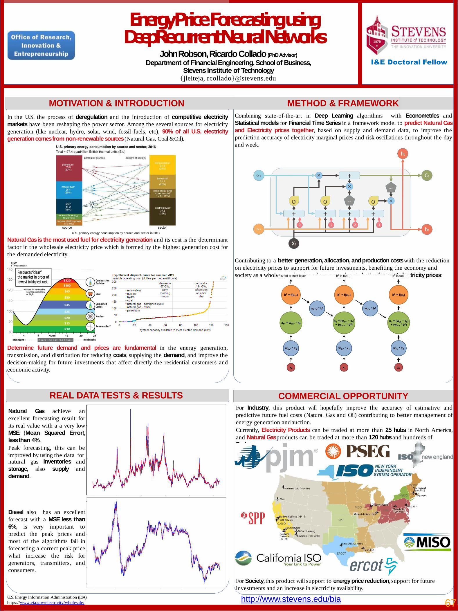
Energy Price Forecasting using Deep Recurrent NeuralNetworks
John Robson, Ricardo Collado (PhD Advisor)
Department of Financial Engineering, School of Business, Stevens Institute of Technology
{jleiteja, rcollado}@stevens.edu
In the U.S. the process of deregulation and the introduction of competitive electricity
markets have been reshaping the power sector. Among the several sources for electricity
generation (like nuclear, hydro, solar, wind, fossil fuels, etc), 90% of all U.S. electricity
generationcomesfrom non-renewablesources(Natural Gas, Coal &Oil).
Determine future demand and prices are fundamental in the energy generation,
transmission, and distribution for reducing costs, supplying the demand, and improve the
decision-making for future investments that affect directly the residential customers and
economic activity.
I&E Doctoral Fellow
REAL DATA TESTS & RESULTS
MOTIVATION & INTRODUCTION METHOD & FRAMEWORK
COMMERCIAL OPPORTUNITY
U.S. Energy Information Administration (EIA)
https://www.eia.gov/electricity/wholesale/
Combining state-of-the-art in Deep Learning algorithms with Econometrics and
Statistical models for Financial Time Series in a framework model to predict Natural Gas
and Electricity prices together, based on supply and demand data, to improve the
prediction accuracy of electricity marginal prices and risk oscillations throughout the day
and week.
e, was developed a new product to better forecast elec
U.S. primary energy consumption by source and sector in 2017
Natural Gas is the most used fuel for electricity generation and its cost is the determinant
factor in the wholesale electricity price which is formed by the highest generation cost for
the demanded electricity.Contributing to a better generation, allocation, and production costs with the reduction
on electricity prices to support for future investments, benefiting the economy and
society as a whol tricity prices:
Natural Gas achieve an
excellent forecasting result for
its real value with a a very low
MSE (Mean Squared Error),
lessthan 4%.
Peak forecasting, this can be
improved by using the data fornatural gas inventories and
storage, also supply and
demand.
Diesel also has an excellent
forecast with a MSE less than
6%, is very important to
predict the peak prices and
most of the algorithms fail in
forecasting a correct peak price
what increase the risk for
generators, transmitters, and
consumers.
For Industry, this product will hopefully improve the accuracy of estimative and
predictive future fuel costs (Natural Gas and Oil) contributing to better management of
energy generation and auction.
Currently, Electricity Products can be traded at more than 25 hubs in North America,
and Natural Gasproducts can be traded at more than 120 hubsand hundreds of
Brokers.
For Society, this product will support to energy price reduction, support for future
investments and an increase in electricity availability.
http://www.stevens.edu/bia 67
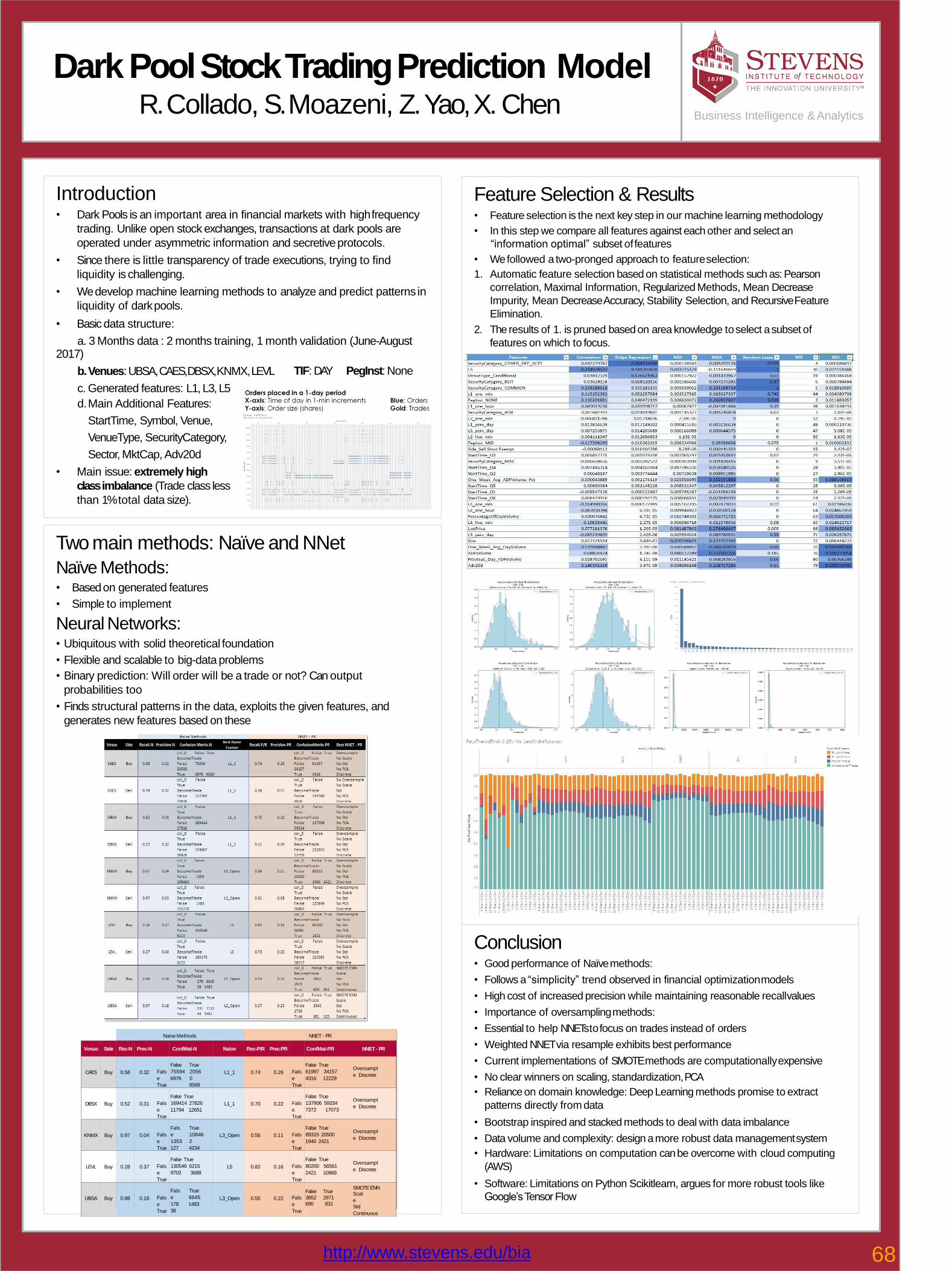
Dark Pool Stock Trading Prediction ModelR. Collado, S. Moazeni, Z. Yao, X. Chen
Feature Selection & Results• Feature selection is the next key step in our machine learning methodology
• In this step we compare all features against each other and select an
“information optimal” subset offeatures
• We followed a two-pronged approach to featureselection:
1. Automatic feature selection based on statistical methods such as: Pearson
correlation, Maximal Information, Regularized Methods, Mean Decrease
Impurity, Mean Decrease Accuracy, Stability Selection, and RecursiveFeature
Elimination.
2. The results of 1. is pruned based on area knowledge toselect a subset of
features on which to focus.
Conclusion• Good performance of Naïvemethods:
• Follows a “simplicity” trend observed in financial optimizationmodels
• High cost of increased precision while maintaining reasonable recallvalues
• Importance of oversamplingmethods:
• Essential to help NNETs tofocus on trades instead of orders
• Weighted NNET via resample exhibits best performance
• Current implementations of SMOTE methods are computationallyexpensive
• No clear winners on scaling, standardization,PCA
• Reliance on domain knowledge: Deep Learning methods promise to extract
patterns directly from data
• Bootstrap inspired and stacked methods to deal with data imbalance
• Data volume and complexity: design a more robust data managementsystem
• Hardware: Limitations on computation can be overcome with cloud computing
(AWS)
• Software: Limitations on Python Scikitlearn, argues for more robust tools like
Google’s Tensor Flow
Business Intelligence & Analytics
http://www.stevens.edu/bia
Introduction• Dark Pools is an important area in financial markets with highfrequency
trading. Unlike open stock exchanges, transactions at dark pools are
operated under asymmetric information and secretiveprotocols.
• Since there is little transparency of trade executions, trying to find
liquidity is challenging.
• We develop machine learning methods to analyze and predict patterns in
liquidity of darkpools.
• Basic data structure:
a. 3 Months data : 2 months training, 1 month validation (June-August
TIF: DAY PegInst:None
2017)
b.Venues: UBSA, CAES, DBSX, KNMX,LEVL
c. Generated features: L1, L3, L5
d.Main Additional Features:
StartTime, Symbol, Venue,
VenueType, SecurityCategory,
Sector, MktCap, Adv20d
• Main issue: extremely high
class imbalance (Trade class less
than 1% total data size).
Two main methods: Naïve and NNet
Naïve Methods:• Based on generated features
• Simple to implement
Neural Networks:• Ubiquitous with solid theoretical foundation
• Flexible and scalable to big-data problems
• Binary prediction: Will order will be a trade or not? Can output
probabilities too
• Finds structural patterns in the data, exploits the given features, and
generates new features based on these
Naïve Methods NNET - PR
Venue Side Rec-N Prec-N ConfMat-N Naïve Rec-P/R Prec-PR ConfMat-PR NNET - PR
CAES Buy 0.58 0.32 Fals
e
True
False
75594
6976
True
2056
0
9569
L1_1 0.74 0.26 Fals
e
True
False True
61997 34157
4316 12229
Oversampl
e Discrete
DBSX Buy 0.52 0.31 Fals
e
True
False True
169414 27826
11794 12651L1_1 0.70 0.22 Fals
e
True
False True
137906 59334
7372 17073
Oversampl
e Discrete
KNMX Buy 0.97 0.04 Fals
e
True
Fals
e
1353
127
True
10846
2
4234
L3_Open 0.56 0.11 Fals
e
True
False True
89315 20500
1940 2421
Oversampl
e Discrete
LEVL Buy 0.28 0.37 Fals
e
True
False True
130546 6215
9702 3688L5 0.82 0.16 Fals
e
True
False True
80200 56561
2421 10969
Oversampl
e Discrete
UBSA Buy 0.98 0.18 Fals
e
True
Fals
e
178
38
True
6645
1483L3_Open 0.55 0.22 Fals
e
True
False True
3852 2971
690 831
SMOTEENNScal
e
Std
Continuous
68
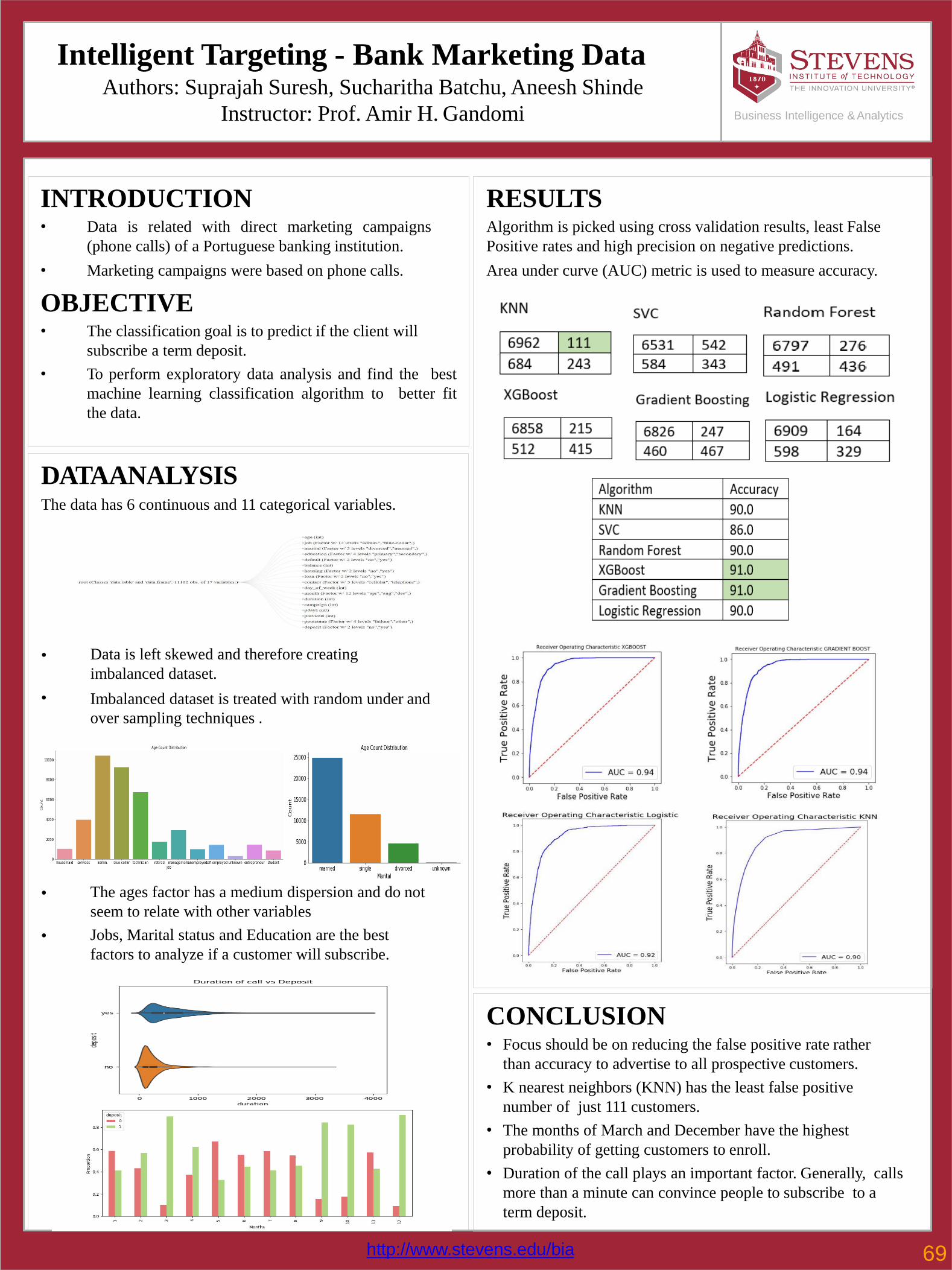
Intelligent Targeting - Bank Marketing DataAuthors: Suprajah Suresh, Sucharitha Batchu, Aneesh Shinde
Instructor: Prof. Amir H. Gandomi
RESULTSAlgorithm is picked using cross validation results, least False
Positive rates and high precision on negative predictions.
Area under curve (AUC) metric is used to measure accuracy.
INTRODUCTION• Data is related with direct marketing campaigns
(phone calls) of a Portuguese banking institution.
• Marketing campaigns were based on phone calls.
OBJECTIVE• The classification goal is to predict if the client will
subscribe a term deposit.
• To perform exploratory data analysis and find the best
machine learning classification algorithm to better fit
the data.
DATAANALYSISThe data has 6 continuous and 11 categorical variables.
•
•
Data is left skewed and therefore creating
imbalanced dataset.
Imbalanced dataset is treated with random under and
over sampling techniques .
•
•
The ages factor has a medium dispersion and do not
seem to relate with other variables
Jobs, Marital status and Education are the best
factors to analyze if a customer will subscribe.
CONCLUSION• Focus should be on reducing the false positive rate rather
than accuracy to advertise to all prospective customers.
• K nearest neighbors (KNN) has the least false positive
number of just 111 customers.
• The months of March and December have the highest
probability of getting customers to enroll.
• Duration of the call plays an important factor. Generally, calls
more than a minute can convince people to subscribe to a
term deposit.
Business Intelligence & Analytics
http://www.stevens.edu/bia 69
Related Documents


