A smoothed NR neural network for solving nonlinear convex programs with second-order cone constraints

Information Sciences 268 (2014) 255–270

Contents lists available at ScienceDirect

Information Sciences

journal homepage: www.elsevier .com/locate / ins

A smoothed NR neural network for solving nonlinear convexprograms with second-order cone constraints

0020-0255/$ - see front matter � 2013 Elsevier Inc. All rights reserved.http://dx.doi.org/10.1016/j.ins.2013.10.017

⇑ Corresponding author. Address: National Center Theoretical Sciences, Taipei Office, Taiwan. Tel.: +886 2 77346641; fax: +886 2 29332342.E-mail addresses: [email protected] (X. Miao), [email protected] (J.-S. Chen), [email protected] (C.-H. Ko).

1 The author’s work is also supported by National Young Natural Science Foundation (No. 11101302) and The Seed Foundation of Tianjin Unive60302041).

2 The author’s work is supported by National Science Council of Taiwan.

Xinhe Miao a,1, Jein-Shan Chen b,⇑,2, Chun-Hsu Ko c

a Department of Mathematics, School of Science, Tianjin University, Tianjin 300072, PR Chinab Department of Mathematics, National Taiwan Normal University, Taipei 11677, Taiwanc Department of Electrical Engineering, I-Shou University, Kaohsiung 84001, Taiwan

a r t i c l e i n f o

Article history:Received 2 January 2012Received in revised form 22 June 2013Accepted 16 October 2013Available online 24 October 2013

Keywords:Merit functionNeural networkNR functionSecond-order coneStability

a b s t r a c t

This paper proposes a neural network approach for efficiently solving general nonlinearconvex programs with second-order cone constraints. The proposed neural network modelwas developed based on a smoothed natural residual merit function involving an uncon-strained minimization reformulation of the complementarity problem. We study the exis-tence and convergence of the trajectory of the neural network. Moreover, we show somestability properties for the considered neural network, such as the Lyapunov stability,asymptotic stability, and exponential stability. The examples in this paper provide a furtherdemonstration of the effectiveness of the proposed neural network. This paper can beviewed as a follow-up version of [20,26] because more stability results are obtained.

� 2013 Elsevier Inc. All rights reserved.

1. Introduction

In this paper, we are interested in finding a solution to the following nonlinear convex programs with second-order coneconstraints (henceforth SOCP):

min f ðxÞs:t: Ax ¼ b

�gðxÞ 2 K

ð1Þ

where A 2 Rm�n has full row rank, b 2 Rm, f : Rn ! R; g ¼ ½g1; . . . ; gl�T : Rn ! Rl with f and gi’s being two order continuous

differentiable and convex on Rn, and K is a Cartesian product of second-order cones (also called Lorentz cones), expressedas

K ¼ Kn1 �Kn2 � � � � �KnN

with N, n1, . . . , nN P 1, n1 + � � � + nN = l and

Kni :¼ fðxi1; xi2; . . . ; xiniÞT 2 Rni j kðxi2; . . . ; xini

Þk 6 xi1g:

rsity (No.

256 X. Miao et al. / Information Sciences 268 (2014) 255–270

Here, k � k denotes the Euclidean norm and K1 means the set of nonnegative reals Rþ. In fact, the problem (1) is equivalent tothe following variational inequality problem, which is to find x 2 D satisfying

hrf ðxÞ; y� xiP 0; 8y 2 D;

where D ¼ fx 2 RnjAx ¼ b; �gðxÞ 2 Kg. Many problems in the engineering, transportation science, and economics commu-nities can be solved by transforming the original problems into the mentioned convex optimization problems or variationalinequality problems, see [1,7,10,17,23].

Many studies have proposed computational approaches to solve convex optimization problems. Examples of these meth-ods include the interior-point method [29], merit function method [5,16], Newton method [18,25], and projection method[10]. However, real-time solutions are imperative in many applications, such as force analysis in robot grasping and controlapplications. The traditional optimization methods may not be suitable for these applications because of stringent compu-tational time requirements. Therefore, a feasible and efficient method is required to solve real-time optimization problems.The neural network method is an ideal method for solving real-time optimization problems. Compared with previous meth-ods, the neural network method has an advantage in solving real-time optimization problems. Hence, researchers havedeveloped many continuous-time neural networks for constrained optimization problems. The literature contains manystudies on neural networks for solving real-time optimization problems, please see [4,9,12,14,15,19–22,27,30–34,36] andreferences therein.

Neural networks stemmed back from McCulloch and Pitts’ pioneering work a half century ago, and neural networks werefirst introduced to the optimization domain in the 1980s [13,28]. The essence of neural network method for optimization [6]is to establish a nonnegative Lyapunov function (or energy function) and a dynamic system that represents an artificial neu-ral network. This dynamic system usually adopts the form of a first-order ordinary differential equation. For an initial point,the neural network is likely to approach its equilibrium point, which corresponds to the solution to the considered optimi-zation problem.

This paper presents a neural network method to solve general nonlinear convex programs with second-order cone con-straints. In particular, we consider the Karush–Kuhn–Tucker (KKT) optimality conditions of the problem (1), which can betransformed into a second-order cone complementarity problems (SOCCP), as well as some equality constraints. Followinga reformulation of the complementarity problem, an unconstrained optimization problem is formulated. A smoothed naturalresidual (NR) complementarity function is then used to construct a Lyapunov function and a neural network model. At thesame time, we show the existence and convergence of the solution trajectory for the dynamic system. This study also inves-tigates the stability results, such as the Lyapunov stability, the asymptotic stability, and the exponential stability. We want topoint out that the optimization problem considered in this paper is more general than the one studied in [20] where g(x) = �xis investigated therein. From [20], for solving the specific SOCP (i.e., g(x) = �x), we know that the neural network based on thecone projection function has better performance than the one based on the Fischer–Burmeister function in most cases (ex-cept for some oscillating cases). In light of considering this phenomenon, we employ a neural network model based on thecone projection function for a more general SOCP. Thus, this paper can be viewed as a follow-up of [20] in this sense. Nev-ertheless, the neural network model studied here is not exactly the same as the one considered in [20]. More specifically, weconsider a neural network based on the smoothed NR function which was studied in [16]. Why do we make such a change?As in Section 4, we can establish various stability results, including exponential stability for the proposed neural networkthat were not achieved in [20]. In addition, the second neural network studied in [27] (for various types of problems) is alsosimilar to the proposed network. Again, the stability is not guaranteed in that study, but three stabilities are proved here.

The remainder of this paper is organized as follows. Section 2 presents stability concepts and provides related results.Section 3 describes the neural network architecture, which is based on the smoothed NR function, to solve the problem(1). Section 4 presents the convergence and stability results of the proposed neural network. Section 5 shows the simulationresults of the new method. Finally, Section 6 gives the conclusion of this paper.

2. Preliminaries

In this section, we briefly recall background materials of the ordinary differential equation (ODE) and some stability con-cepts regarding the solution of ODE. We also present some related results that play an essential role in the subsequentanalysis.

Let H : Rn ! Rn be a mapping. The first order differential equation (ODE) means

dudt¼ HðuðtÞÞ; uðt0Þ ¼ u0 2 Rn: ð2Þ

We start with the existence and uniqueness of the solution of Eq. (2). Then, we introduce the equilibrium point of (2) anddefine various stabilities. All of these materials can be found in a typical ODE textbook, such as [24].

Lemma 2.1 (The existence and uniqueness 21, Theorem 2.5). Assume that H : Rn ! Rn is a continuous mapping. Then forarbitrary t0 P 0 and u0 2 Rn, there exists a local solution u(t), t 2 [t0,s) to (2) for some s > t0. Furthermore, if H is locally Lipschitzcontinuous at u0, then the solution is unique; if H is Lipschitz continuous in Rn , then s can be extended to 1.

X. Miao et al. / Information Sciences 268 (2014) 255–270 257

Remark 2.1. For Eq. (2), if a local solution defined on [t0,s) cannot be extended to a local solution on a larger interval [t0,s1),where s1 > s, then it is called a maximal solution, and this interval [t0,s) is the maximal interval of existence. It is obviousthat an arbitrary local solution has an extension to a maximal one.

Lemma 2.2 (21, Theorem 2.6). Let H : Rn ! Rn be a continuous mapping. If u(t) is a maximal solution, and [t0,s) is the maximalinterval of existence associated with u0 and s < +1, then limt"sku(t)k = +1.

For the first-order differential Eq. (2), a point u� 2 Rn is called an equilibrium point of (2) if H(u⁄) = 0. If there is a neigh-borhood X # Rn of u⁄ such that H(u⁄) = 0 and H(u) – 0 for any u 2Xn{u⁄}, then u⁄ is called an isolated equilibrium point. Thefollowing are definitions of various stabilities, and related materials can be found in [21,24,27].

Definition 2.1 (Lyapunov stability and Asymptotic stability). Let u(t) be a solution to Eq. (2).

(a) An isolated equilibrium point u⁄ is Lyapunov stable (or stable in the sense of Lyapunov) if for any u0 = u(t0) and e > 0,there exists a d > 0 such that

ku0 � u�k < d ) kuðtÞ � u�k < e for t P t0:

(b) Under the condition that an isolated equilibrium point u⁄ is Lyapunov stable, u⁄ is said to be asymptotically stable if ithas the property that if ku0 � u⁄k < d, then u(t) ? u⁄ as t ?1.

Definition 2.2 (Lyapunov function). Let X # Rn be an open neighborhood of �u. A continuously differentiable functiong : Rn ! R is said to be a Lyapunov function (or energy function) at the state �u (over the set X) for Eq. (2) if

gð�uÞ ¼ 0;gðuÞ > 0 8u 2 X n f�ug;dgðuðtÞÞ

dt 6 0; 8u 2 X:

8><>:

The following Lemma shows the relationship between stabilities and a Lyapunov function, see [3,8,35].

Lemma 2.3.

(a) An isolated equilibrium point u⁄ is Lyapunov stable if there exists a Lyapunov function over some neighborhood X of u⁄.(b) An isolated equilibrium point u⁄ is asymptotically stable if there exists a Lyapunov function over some neighborhood X of u⁄

that satisfies

dgðuðtÞÞdt

< 0; 8u 2 X n fu�g:

Definition 2.3 (Exponential stability). An isolated equilibrium point u⁄ is exponentially stable for Eq. (2) if there exist x < 0,j > 0, d > 0 such that arbitrary solution u(t) to Eq. (2), with the initial condition u(t0) = u0, ku0 � u⁄k < d, is defined on [0,1)and satisfies

kuðtÞ � u�k 6 jextkuðt0Þ � u�k; t P t0:

From the above definitions, it is obvious that exponential stability is asymptotic stable.

3. NR neural network model

This section shows how the dynamic system in this study was formed. As mentioned previously, the key steps in the neu-ral network method lie in constructing the dynamic system and Lyapunov function. To this end, we first look into the KKTconditions of the problem (1) which are presented as below:

rf ðxÞ � AT yþrgðxÞz ¼ 0;z 2 K; �gðxÞ 2 K; zT gðxÞ ¼ 0;Ax� b ¼ 0;

8><>: ð3Þ

where y 2 Rm,rg(x) denotes the gradient matrix of g. According to the KKT condition, it is well known that if the problem (1)satisfies Slater’s condition, which means there exists a strictly feasible point for (1), i.e., there exists an x 2 Rn such that�gðxÞ 2 intðKÞ and Ax = b. Then x⁄ is a solution of the problem (1) if and only if there exist y⁄, z⁄ such that (x⁄,y⁄,z⁄) satisfiesthe KKT conditions (3). Hence, we assume that the problem (1) satisfies the Slater’s condition in this paper.

258 X. Miao et al. / Information Sciences 268 (2014) 255–270

The following paragraphs provide a brief review of particular properties of the spectral factorization with respect to a sec-ond-order cone, which will be used in the subsequent analysis. Spectral factorization is one of the basic concepts in Jordanalgebra. For more details, see [5,11,25].

For any vector z ¼ ðz1; z2Þ 2 R� Rl�1ðl P 2Þ, its spectral factorization with respect to the second-order cone K is defined as

z ¼ k1e1 þ k2e2;

where ki = z1 + (�1)ikz2k, (i = 1,2) are the spectral values of z, and

ei ¼12 ð1; ð�1Þi zi

kzikÞ; z2 – 0

12 ð1; ð�1ÞiwÞ; z2 ¼ 0

(

with w 2 Rl�1 such that kwk = 1. The terms e1, e2 are called the spectral vectors of z. The spectral values of z and the vector zhave the following properties: for any z 2 Rl, there have k1 6 k2 and

k1 P 0 () z 2 K:

Now we review the concept of metric projection onto K. For arbitrary element z 2 Rl, the metric projection of z onto K is de-noted by PKðzÞ and defined as

PKðzÞ :¼ arg minw2Kkz�wk:

Combining the spectral decomposition of z with the metric projection of z onto K yields the expression of metric projectionPKðzÞ in [11]:

PKðzÞ ¼maxf0; k1ge1 þmaxf0; k2ge2:

The projection function PK has the following property, which is called the Projection Theorem (see [2]).

Lemma 3.1. Let X be a closed convex set of Rn. Then, for all x; y 2 Rn and any z 2X,

ðx� PXðxÞÞTðPXðxÞ � zÞP 0 and kPXðxÞ � PXðyÞk 6 kx� yk:

Given the definition of the projection, suppose z+ denotes the metric projection PKðzÞ of z 2 Rl onto K. Then, the naturalresidual (NR) function is given as follows [11]:

UNRðx; yÞ :¼ x� ðx� yÞþ 8x; y 2 Rl:

The NR function is a popular SOC-complementarity function, i.e.,

UNRðx; yÞ ¼ 0() x 2 K; y 2 K and hx; yi ¼ 0:

Because of the non-differentiability of UNR, we consider a class of smoothed NR complementarity function. To this end, weemploy a continuously differentiable convex function g : R! R such that

lima!�1

gðaÞ ¼ 0; lima!1ðgðaÞ � aÞ ¼ 0 and 0 < g0ðaÞ < 1: ð4Þ

What kind of functions satisfies the condition (4)? Here we present two examples:

gðaÞ ¼ffiffiffiffiffiffiffiffiffiffiffiffiffiffia2 þ 4p

þ a2

and gðaÞ ¼ lnðea þ 1Þ:

Suppose z = k1e1 + k2e2, where ki and ei (i = 1,2) are the spectral values and spectral vectors of z, respectively. By applying thefunction g, we define the following function:

PlðzÞ :¼ lgk1

l

� �e1 þ lg

k2

l

� �e2: ð5Þ

Fukushima et al. [11] show that Pl is smooth for any l > 0; moreover Pl is a smoothing function of the projection PK, i.e.,liml#0Pl ¼ PK. Hence, a smoothed NR complementarity function is given in the form of

Ulðx; yÞ :¼ x� Plðx� yÞ:

In particular, from [11, Proposition 5.1], there exists a positive constant c > 0 such that

kUlðx; yÞ �UNRðx; yÞk 6 cl

for any l > 0 and ðx; yÞ 2 Rn � Rn.

X. Miao et al. / Information Sciences 268 (2014) 255–270 259

Now we look into the KKT conditions (3) of the problem (1). Let

Lðx; y; zÞ ¼ rf ðxÞ � AT yþrgðxÞz; HðuÞ :¼

lAx� b

Lðx; y; zÞUlðz;�gðxÞÞ

26664

37775

and

WlðuÞ :¼ 12kHðuÞk2 ¼ 1

2kUlðz;�gðxÞÞk2 þ 1

2kLðx; y; zÞk2 þ 1

2kAx� bk2 þ 1

2l2;

where u ¼ ðl; xT ; yT ; zTÞT 2 Rþ � Rn � Rm � Rl. It is known that Wl(u) serves as a smoothing function of the merit functionWNR which means the KKT conditions (3) are shown to be equivalent to the following unconstrained minimization problemvia the merit function approach:

min WlðuÞ :¼ 12kHðuÞk2

: ð6Þ

Theorem 3.1.

(a) Let Pl be defined by (5). Then, r Pl(z) and I �rPl(z) are positive definite for any l > 0 and z 2 Rl.(b) Let Wl be defined as in (6). Then, the smoothed merit function Wl is continuously differentiable everywhere withrWl(u) =rH(u)H(u) where

rHðuÞ ¼

1 0 0 � @PlðzþgðxÞÞ@l

� �T

0 AT r2f ðxÞ þ r2g1ðxÞ þ � � � þ r2glðxÞ �rxPlðzþ gðxÞÞ0 0 �A 00 0 rgðxÞT I �rzPlðzþ gðxÞÞ

2666664

3777775: ð7Þ

Proof. Form the proof of [16, Proposition 3.1], it is clear that rPl(z) and I �rPl(z) are positive definite for any l > 0 andz 2 Rl. With the help of the definition of the smoothed merit function Wl, part (b) easily follows from the chain rule. h

In light of the main ideas for constructing artificial neural networks (see [6] for details), we establish a specific first orderordinary differential equation, i.e., an artificial neural network. More specifically, based on the gradient of the objective func-tion Wl in minimization problem (6), we propose the neural network for solving the KKT system (3) of nonlinear SOCP (1)with the following differential equation:

duðtÞdt¼ �qrWlðuÞ; uðt0Þ ¼ u0; ð8Þ

where q > 0 is a time scaling factor. In fact, if s = qt, then duðtÞdt ¼ q duðsÞ

ds . Hence, it follows from (8) that duðsÞds ¼ �rWlðuÞ. In view

of this, for simplicity and convenience, we set q = 1 in this paper. Indeed, the dynamic system (8) can be realized by an archi-tecture with the cone projection function shown in Fig. 1. Moreover, the architecture of this artificial neural network is cat-egorized as a ‘‘recurrent’’ neural network according to the classifications of artificial neural networks as in [6, Chapter 2.3.1].The circuit for (8) requires n + m + l + 1 integrators, n processors for rf(x), l processors for g(x), ln processors for rg(x),(l + 1)2n processors for r2f ðxÞ þ

Pli¼1r2giðxÞ, 1 processor for Ul, 1 processor for @Pl

@l ;n processors for rxPl,l processors forrzPl, n2 + 4mn + 3ln + l2 + l connection weights and some summers.

4. Stability analysis

In this section, in order to study the stability issues of the proposed neural network (8) for solving the problem (1), wefirst make an assumption that will be required in our subsequent analysis.

Assumption 4.1.

(a) The problem (1) satisfies the Slater’s condition.(b) The matrix r2 f(x) +r2g1(x) + � � � +r2gl(x) is positive definite for each x.

Here we say a few words about Assumption 4.1(a and b). The Slater’s condition is a standard condition that is widely usedin optimization field. Assumption 4.1(b) seems stringent at first glance. Indeed, since f and gi’s are two order continuouslydifferentiable and convex functions on Rn, if there exists at least one function which is strictly convex among these functions,then Assumption 4.1(b) is guaranteed.

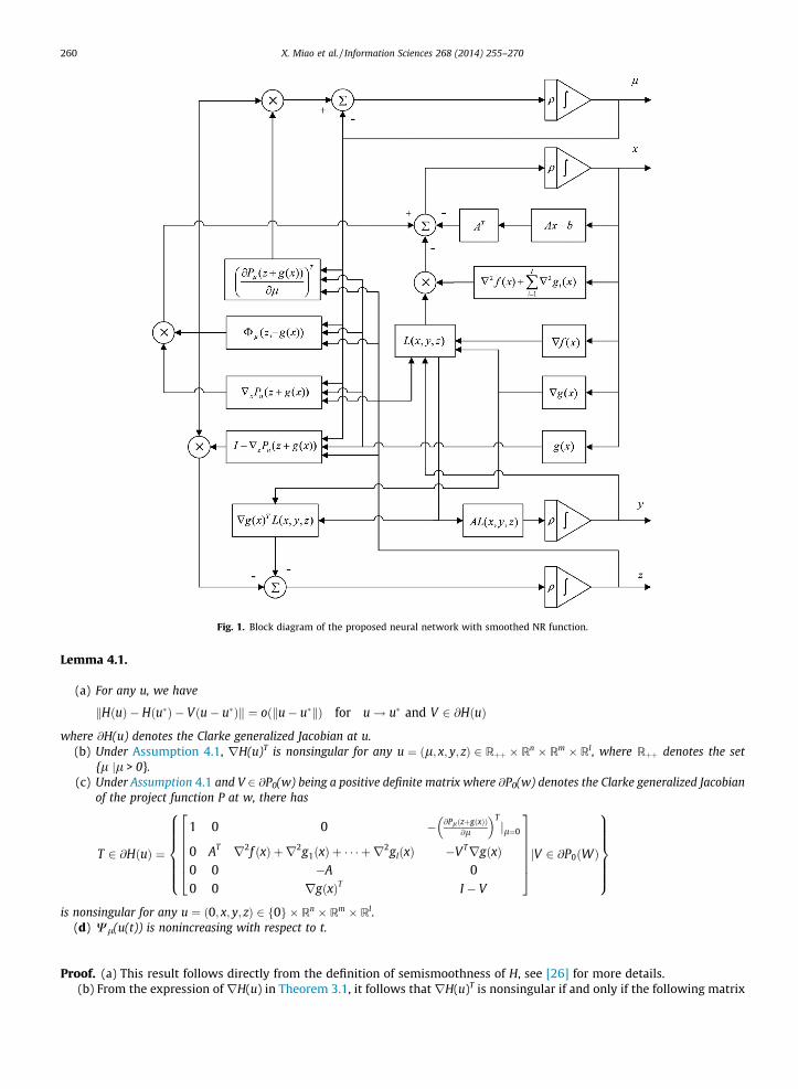
Fig. 1. Block diagram of the proposed neural network with smoothed NR function.

260 X. Miao et al. / Information Sciences 268 (2014) 255–270

Lemma 4.1.

(a) For any u, we have

kHðuÞ � Hðu�Þ � Vðu� u�Þk ¼ oðku� u�kÞ for u! u� and V 2 @HðuÞ

where @H(u) denotes the Clarke generalized Jacobian at u.(b) Under Assumption 4.1, rH(u)T is nonsingular for any u ¼ ðl; x; y; zÞ 2 Rþþ � Rn � Rm � Rl, where Rþþ denotes the set

{l jl > 0}.(c) Under Assumption 4.1 and V 2 @P0(w) being a positive definite matrix where @P0(w) denotes the Clarke generalized Jacobian

of the project function P at w, there has

T 2 @HðuÞ ¼

1 0 0 � @PlðzþgðxÞÞ@l

� �Tjl¼0

0 AT r2f ðxÞ þ r2g1ðxÞ þ � � � þ r2glðxÞ �VTrgðxÞ0 0 �A 00 0 rgðxÞT I � V

2666664

3777775jV 2 @P0ðWÞ

8>>>>><>>>>>:

9>>>>>=>>>>>;

is nonsingular for any u ¼ ð0; x; y; zÞ 2 f0g � Rn � Rm � Rl.(d) Wl(u(t)) is nonincreasing with respect to t.

Proof. (a) This result follows directly from the definition of semismoothness of H, see [26] for more details.(b) From the expression ofrH(u) in Theorem 3.1, it follows thatrH(u)T is nonsingular if and only if the following matrix

X. Miao et al. / Information Sciences 268 (2014) 255–270 261

M :¼A 0 0

r2f ðxÞ þ r2g1ðxÞ þ � � � þ r2glðxÞ �AT rgðxÞ�rxPlðzþ gðxÞÞT 0 ðI �rzPlðzþ gðxÞÞÞT

264

375

is nonsingular. Suppose v ¼ ðx; y; zÞ 2 Rn � Rm � Rl. To show the nonsingularity of M, it is enough to prove that

Mv ¼ 0 ) x ¼ 0; y ¼ 0 and z ¼ 0:

Because �rxPl(z + g(x))T = �rPl(w)Tr g(x)T, where w ¼ zþ gðxÞ 2 Rl, from Mv = 0, we have

Ax ¼ 0; ðr2f ðxÞ þ r2g1ðxÞ þ � � � þ r2glðxÞÞx� AT yþrgðxÞz ¼ 0 ð9Þ

and

�rPlðwÞTrgðxÞT xþ ðI �rPlðwÞÞT z ¼ 0: ð10Þ

From (9), it follows that

xTðr2f ðxÞ þ r2g1ðxÞ þ � � � þ r2glðxÞÞxþ ðrgðxÞT xÞTz ¼ 0: ð11Þ

Moveover, Eq. (10) and Theorem 3.1 yield

rgðxÞT x ¼ ðrPlðwÞTÞ�1ðI �rPlðwÞÞT z: ð12Þ

Combining (11) and (12) and Theorem 3.1, under the condition of Assumption 4.1, it is not hard to obtain that x = 0 and z = 0.By looking at Eq. (9) again, since A is full row rank, we have y = 0. Therefore, rH(u)T is nonsingular.

(c) The proof of Part (c) is similar to that of Part (b), in which the only option is to replace rPl(w) with V 2 @ P0(w).(d) According to the definition of Wl(u(t)) and Eq. (8), it is clear that

dWlðuðtÞÞdt

¼ rWlðuðtÞÞduðtÞ

dt¼ �qkrWlðuðtÞÞk2

6 0:

Consequently, Wl(u(t)) is nonincreasing with respect to t. h

Proposition 4.1. Assume that rH(u) is nonsingular for any u 2 Rþ � Rn � Rm � Rl. Then,

(a) (x⁄, y⁄, z⁄) satisfies the KKT conditions (3) if and only if (0,x⁄, y⁄, z⁄) is an equilibrium point of the neural network (8);(b) Under the Slater’s condition, x⁄ is a solution to the problem (1) if and only if (0,x⁄, y⁄, z⁄) is an equilibrium point of the neural

network (8).

Proof. (a) Because U0 = UNR when l = 0, it follows that (x⁄,y⁄,z⁄) satisfies the KKT conditions (3) if and only if H(u⁄) = 0,where u⁄ = (0,x⁄,y⁄,z⁄)T. Since rH(u) is nonsingular, we have that H(u⁄) = 0 if and only if r Wl(u⁄) =rH(u⁄)TH(u⁄) = 0. Thus,the desired result follows.

(b) Under the Slater’s condition, it is well known that x⁄ is a solution of the problem (1) if and only if there exist y⁄ and z⁄

such that (x⁄,y⁄,z⁄) satisfying the KKT conditions (3). Hence, according to Part (a), it follows that (0,x⁄,y⁄,z⁄) is an equilibriumpoint of the neural network (8). h

The next result addresses the existence and uniqueness of the solution trajectory of the neural network (8).

Theorem 4.1.

(a) For any initial point u0 = u(t0), there exists a unique continuously maximal solution u(t) with t 2 [t0,s) for the neural net-work (8), where [t0,s) is the maximal interval of existence.

(b) If the level set Lðu0Þ :¼ fujWlðuÞ 6 Wlðu0Þg is bounded, then s can be extended to +1.

Proof. This proof is exactly the same as the proof of [27, Proposition 3.4], and therefore omitted here. h

Theorem 4.2. Assume that rH(u) is nonsingular and that u⁄ is an isolated equilibrium point of the neural network (8). Then thesolution of the neural network (8) with any initial point u0 is Lyapunov stable.

Proof. From Lemma 2.3, we only need to argue that there exists a Lyapunov function over some neighborhood X of u⁄. Now,we consider the smoothed merit function

WlðuÞ ¼12kHðuÞk2:

262 X. Miao et al. / Information Sciences 268 (2014) 255–270

Since u⁄ is an isolated equilibrium point of (8), there is a neighborhood X of u⁄ such that

rWlðu�Þ ¼ 0 and rWlðuðtÞÞ– 0; 8uðtÞ 2 X n fu�g:

By the nonsingularity of rH(u) and the definition of Wl, it is easy to obtain that Wl(u⁄) = 0. From the definition of Wl, weclaim that Wl(u(t)) > 0 for any u(t) 2Xn{u⁄}, where X is a neighborhood of u⁄. Suppose not, namely, Wl(u(t)) = 0. It followsthat H(u(t)) = 0. Then, we haverWl(u(t)) = 0 which contradicts with the assumption that u⁄ is an isolated equilibrium pointof (8). Thus, Wl(u(t)) > 0 for any u(t) 2Xn{u⁄}. Furthermore, by the proof of Lemma 4.1(d), we know that for any u(t) 2X

dWlðuðtÞÞdt

¼ rWlðuðtÞÞduðtÞ

dt¼ �qkrWlðuðtÞÞk2

6 0: ð13Þ

Consequently, the function Wl is a Lyapunov function over X. This implies that u⁄ is Lyapunov stable for the neural network(8). h

Theorem 4.3. Assume thatrH(u) is nonsingular and that u⁄ is an isolated equilibrium point of the neural network (8). Then u⁄ isasymptotically stable for neural network (8).

Proof. From the proof of Theorem 4.2, we consider again the Lyapunov function Wl. By Lemma 2.3 again, we only need toverify that the Lyapunov function Wl over some neighborhood X of u⁄ satisfies

dWlðuðtÞÞdt

< 0; 8uðtÞ 2 X n fu�g: ð14Þ

In fact, by using (13) and the definition of the isolated equilibrium point, it is not hard to check that the Eq. (14) is true.Hence, u⁄ is asymptotically stable. h

Theorem 4.4. Assume that u⁄ is an isolated equilibrium point of the neural network (8). If rH(u)T is nonsingular for anyu ¼ ðl; x; y; zÞ 2 Rþ � Rn � Rm � Rl, then u⁄ is exponentially stable for the neural network (8).

Proof. From the definition of H(u), we know that H is semismooth. Hence, by Lemma 4.1, we have

HðuÞ ¼ Hðu�Þ þ rHðuðtÞÞTðu� u�Þ þ oðku� u�kÞ; 8u 2 X n fu�g; ð15Þ

where rH(u(t))T 2 @H(u(t)) and X is a neighborhood of u⁄. Now, we let

gðuðtÞÞ ¼ kuðtÞ � u�k2; t 2 ½t0;1Þ:

Then, we have

dgðuðtÞÞdt

¼ 2ðuðtÞ � u�ÞT duðtÞdt¼ �2qðuðtÞ � u�ÞTrWlðuðtÞÞ ¼ �2qðuðtÞ � u�ÞTrHðuÞHðuÞ: ð16Þ

Substituting Eq. (15) into Eq. (16) yields

dgðuðtÞÞdt

¼ �2qðuðtÞ � u�ÞTrHðuðtÞÞðHðu�Þ þ rHðuðtÞÞTðuðtÞ � u�Þ þ oðkuðtÞ � u�kÞÞ

¼ �2qðuðtÞ � u�ÞTrHðuðtÞÞrHðuðtÞÞTðuðtÞ � u�Þ þ oðkuðtÞ � u�k2Þ:

Because rH(u) and rH(u)T are nonsingular, we claim that there exists an j > 0 such that

ðuðtÞ � u�ÞTrHðuÞrHðuÞTðuðtÞ � u�ÞP jkuðtÞ � u�k2: ð17Þ

Otherwise, if (u(t) � u⁄)TrH(u(t))r H(u(t))T(u(t) � u⁄) = 0, it implies that

rHðuðtÞÞTðuðtÞ � u�Þ ¼ 0:

Indeed, from the nonsingularity of H(u), we have u(t) � u⁄ = 0, i.e., u(t) = u⁄which contradicts with the assumption of u⁄ beingan isolated equilibrium point. Consequently, there exists an j > 0 such that (17) holds. Moreover, for o(ku(t) � u⁄k2), there ise > 0 such that o(ku(t) � u⁄k2) 6 e ku(t) � u⁄k2. Hence,

dgðuðtÞÞdt

6 ð�2qjþ eÞkuðtÞ � u�k2 ¼ ð�2qjþ eÞgðuðtÞÞ:

This implies

gðuðtÞÞ 6 eð�2qjþeÞtgðuðt0ÞÞ

Table 1Stability comparisons of neural networks considered in current paper, [20,27].

Current paper [20] [27]

Problem min f ðxÞs:t: Ax ¼ b

�gðxÞ 2 K

min f ðxÞs:t: Ax ¼ b

x 2 K

hFðxÞ; y� xiP 0; 8y 2 CC ¼ fxj hðxÞ ¼ 0;�gðxÞ 2 Kg

ODE Based on smoothed NR-function Based on NR-function and FB-function Based on NR-function and smoothed FB-functionStability Lyapunov (smoothed NR) Lyapunov (NR) Lyapunov (NR)

Asymptotical (smoothed NR) Lyapunov (FB) Asymptotical (NR)Exponential (smoothed NR) asymptotical (FB) Exponential (smoothed FB)

X. Miao et al. / Information Sciences 268 (2014) 255–270 263

which means

kuðtÞ � u�k 6 e�qjþe2kuðt0Þ � u�k:

Thus, u⁄ is exponentially stable for the neural network (8). h

To show the contribution of this paper, we present the stability comparisons of neural networks considered in the currentpaper, [20,27] in Table 1. More convergence comparisons will be presented in the next section. Generally speaking, we estab-lish three stabilities for the proposed neural network, whereas not all three stabilities for the similar neural networks studiedin [20,27] are guaranteed. Why do we choose to investigate the proposed neural network? Indeed, in [20], two neural net-works based on NR function and FB function are considered which does not reach exponential stability. Our target optimi-zation problem is a wider class than the one studied in [20]. In contrast, the smoothed FB has good performance as is shownin [27], but not all the three stabilities are established even though exponential stability is good enough. In light of theseobservations, we decide to look into the smoothed NR function for our problem which turns out to have better theoreticalresults. We summarize their differences in problems format, dynamical model, and stability issues in Table 1.

5. Numerical examples

In order to demonstrate the effectiveness of the proposed neural network, in this section we test several examples for ourneural network (8). The numerical implementation is coded by Matlab 7.0 and the ordinary differential equation solveradopted here is ode23, which uses the Ruge–Kutta (2;3) formula. As mentioned earlier, the parameter q is set to be 1.How is l chosen initially? From Theorem 4.2 in previous section, we know the solution converges with any initial point,we set initial l = 1 in the codes (and of course l ? 0, as seen in the trajectory behavior).

Example 5.1. Consider the following nonlinear convex programming problem:

min eðx1�3Þ2þx22þðx3�1Þ2þðx4�2Þ2þðx5þ1Þ2

s:t: x 2 K5;

Here, we denote f ðxÞ :¼ eðx1�3Þ2þx22þðx3�1Þ2þðx4�2Þ2þðx5þ1Þ2 and g(x) = �x. Then, we compute

Lðx; zÞ ¼ rf ðxÞ þ rgðxÞz ¼ 2f ðxÞ

x1 � 3x2

x3 � 1x4 � 2x5 þ 1

26666664

37777775�

z1

z2

z3

z4

z5

26666664

37777775: ð18Þ

Moreover, let x :¼ ðx1; �xÞ 2 R� R4 and z :¼ ðz1;�zÞ 2 R� R4. Then, the element z � x can be expressed as

z� x :¼ k1e1 þ k2e2

where ki ¼ z1 � x1 þ ð�1Þik�z� �xk and ei ¼ 12 1; ð�1Þi �z��x

k�z��xk

� �ði ¼ 1;2Þ if �z� �x – 0, otherwise ei ¼ 1

2 ð1; ð�1ÞiwÞ with w being anyvector in R4 satisfying kwk = 1. This implies that

Ulðz;�gðxÞÞ ¼ z� Plðzþ gðxÞÞ ¼ z� lgk1

l

� �e1 þ lg

k2

l

� �e2 ð19Þ

with gðaÞ ¼ffiffiffiffiffiffiffiffia2þ4p

þa2 or gðaÞ ¼ lnðea þ 1Þ. Therefore, by Eqs. (18) and (19), we obtain the expression of H(u) as follows:

HðuÞ ¼l

Lðx; zÞUlðz;�gðxÞÞ

264

375:

264 X. Miao et al. / Information Sciences 268 (2014) 255–270

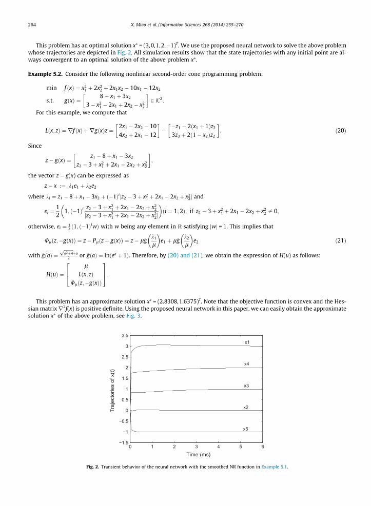
This problem has an optimal solution x⁄ = (3,0,1,2,�1)T. We use the proposed neural network to solve the above problemwhose trajectories are depicted in Fig. 2. All simulation results show that the state trajectories with any initial point are al-ways convergent to an optimal solution of the above problem x⁄.

Example 5.2. Consider the following nonlinear second-order cone programming problem:

min f ðxÞ ¼ x21 þ 2x2

2 þ 2x1x2 � 10x1 � 12x2

s:t: gðxÞ ¼8� x1 þ 3x2

3� x21 � 2x1 þ 2x2 � x2

2

� �2 K2:

For this example, we compute that

Lðx; zÞ ¼ rf ðxÞ þ rgðxÞz ¼2x1 � 2x2 � 104x2 þ 2x1 � 12

� ���z1 � 2ðx1 þ 1Þz2

3z3 þ 2ð1� x2Þz2

� �: ð20Þ

Since

z� gðxÞ ¼z1 � 8þ x1 � 3x2

z2 � 3þ x21 þ 2x1 � 2x2 þ x2

2

� �;

the vector z � g(x) can be expressed as

z� x :¼ k1e1 þ k2e2

where ki ¼ z1 � 8þ x1 � 3x2 þ ð�1Þijz2 � 3þ x21 þ 2x1 � 2x2 þ x2

2j and

ei ¼12

1; ð�1Þi z2 � 3þ x21 þ 2x1 � 2x2 þ x2

2

jz2 � 3þ x21 þ 2x1 � 2x2 þ x2

2j

� �ði ¼ 1;2Þ; if z2 � 3þ x2

1 þ 2x1 � 2x2 þ x22 – 0;

otherwise, ei ¼ 12 ð1; ð�1ÞiwÞ with w being any element in R satisfying jwj = 1. This implies that

Ulðz;�gðxÞÞ ¼ z� Plðzþ gðxÞÞ ¼ z� lgk1

l

� �e1 þ lg

k2

l

� �e2 ð21Þ

with gðaÞ ¼ffiffiffiffiffiffiffiffia2þ4p

þa2 or gðaÞ ¼ lnðea þ 1Þ. Therefore, by (20) and (21), we obtain the expression of H(u) as follows:

HðuÞ ¼l

Lðx; zÞUlðz;�gðxÞÞ

264

375:

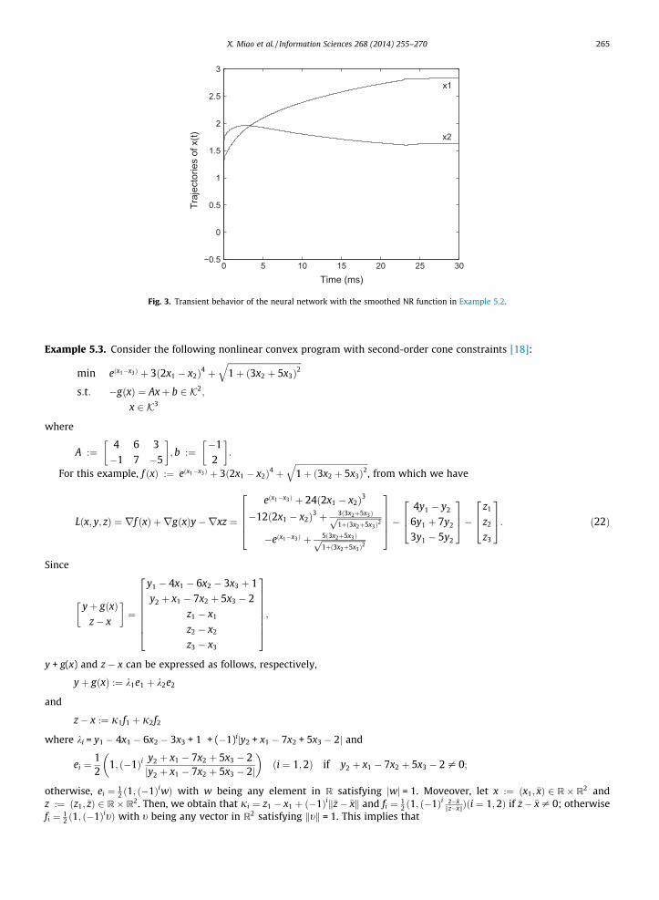
This problem has an approximate solution x⁄ = (2.8308,1.6375)T. Note that the objective function is convex and the Hes-sian matrixr2f(x) is positive definite. Using the proposed neural network in this paper, we can easily obtain the approximatesolution x⁄ of the above problem, see Fig. 3.

0 1 2 3 4 5 6−1.5

−1

−0.5

0

0.5

1

1.5

2

2.5

3

3.5

Time (ms)

Traj

ecto

ries

of x

(t)

x1

x2

x3

x4

x5

Fig. 2. Transient behavior of the neural network with the smoothed NR function in Example 5.1.

0 5 10 15 20 25 30−0.5

0

0.5

1

1.5

2

2.5

3

Time (ms)

Traj

ecto

ries

of x

(t)

x1

x2

Fig. 3. Transient behavior of the neural network with the smoothed NR function in Example 5.2.

X. Miao et al. / Information Sciences 268 (2014) 255–270 265

Example 5.3. Consider the following nonlinear convex program with second-order cone constraints [18]:

min eðx1�x3Þ þ 3ð2x1 � x2Þ4 þffiffiffiffiffiffiffiffiffiffiffiffiffiffiffiffiffiffiffiffiffiffiffiffiffiffiffiffiffiffiffiffiffiffiffi1þ ð3x2 þ 5x3Þ2

qs:t: �gðxÞ ¼ Axþ b 2 K2;

x 2 K3

where

A :¼4 6 3�1 7 �5

� �; b :¼

�12

� �: ffiffiffiffiffiffiffiffiffiffiffiffiffiffiffiffiffiffiffiffiffiffiffiffiffiffiffiffiffiffiffiffiffiffiffiq

For this example, f ðxÞ :¼ eðx1�x3Þ þ 3ð2x1 � x2Þ4 þ 1þ ð3x2 þ 5x3Þ2, from which we have

Lðx; y; zÞ ¼ rf ðxÞ þ rgðxÞy�rxz ¼

eðx1�x3Þ þ 24ð2x1 � x2Þ3

�12ð2x1 � x2Þ3 þ 3ð3x2þ5x3Þffiffiffiffiffiffiffiffiffiffiffiffiffiffiffiffiffiffiffiffiffi1þð3x2þ5x3Þ2p

�eðx1�x3Þ þ 5ð3x2þ5x3Þffiffiffiffiffiffiffiffiffiffiffiffiffiffiffiffiffiffiffiffiffi1þð3x2þ5x3Þ2p

26664

37775�

4y1 � y2

6y1 þ 7y2

3y1 � 5y2

264

375�

z1

z2

z3

264

375: ð22Þ

Since

yþ gðxÞz� x

� �¼

y1 � 4x1 � 6x2 � 3x3 þ 1y2 þ x1 � 7x2 þ 5x3 � 2

z1 � x1

z2 � x2

z3 � x3

26666664

37777775;

y + g(x) and z � x can be expressed as follows, respectively,

yþ gðxÞ :¼ k1e1 þ k2e2

and

z� x :¼ j1f1 þ j2f2

where ki = y1 � 4x1 � 6x2 � 3x3 + 1 + (�1)ijy2 + x1 � 7x2 + 5x3 � 2j and

ei ¼12

1; ð�1Þi y2 þ x1 � 7x2 þ 5x3 � 2jy2 þ x1 � 7x2 þ 5x3 � 2j

� �ði ¼ 1;2Þ if y2 þ x1 � 7x2 þ 5x3 � 2 – 0;

otherwise, ei ¼ 12 ð1; ð�1ÞiwÞ with w being any element in R satisfying jwj = 1. Moveover, let x :¼ ðx1; �xÞ 2 R� R2 and

z :¼ ðz1;�zÞ 2 R� R2. Then, we obtain that ji ¼ z1 � x1 þ ð�1Þik�z� �xk and fi ¼ 12 ð1; ð�1Þi �z��x

k�z��xkÞði ¼ 1;2Þ if �z� �x – 0; otherwisefi ¼ 1

2 ð1; ð�1ÞitÞ with t being any vector in R2 satisfying ktk = 1. This implies that

266 X. Miao et al. / Information Sciences 268 (2014) 255–270

Ulð�Þ ¼y� Plðyþ gðxÞÞ

z� Plðz� xÞ

� �¼

y� lg k1l

� �e1 þ lg k2

l

� �e2

z� lg j1l

� �f1 þ lg j2

l

� �f2

264

375 ð23Þ

with gðaÞ ¼ffiffiffiffiffiffiffiffia2þ4p

þa2 or gðaÞ ¼ lnðea þ 1Þ. Therefore, by (22) and (23), we obtain the expression of H(u) as below:

HðuÞ ¼l

Lðx; y; zÞUlð�Þ

264

375:

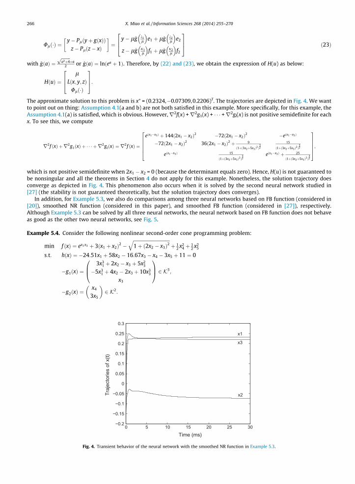
The approximate solution to this problem is x⁄ = (0.2324,�0.07309,0.2206)T. The trajectories are depicted in Fig. 4. We wantto point out on thing: Assumption 4.1(a and b) are not both satisfied in this example. More specifically, for this example, theAssumption 4.1(a) is satisfied, which is obvious. However,r2f(x) +r2g1(x) + � � � +r2gl(x) is not positive semidefinite for eachx. To see this, we compute

r2f ðxÞ þ r2g1ðxÞ þ � � � þ r2glðxÞ ¼ r2f ðxÞ ¼

eðx1�x3Þ þ 144ð2x1 � x2Þ2 �72ð2x1 � x2Þ2 �eðx1�x3Þ

�72ð2x1 � x2Þ2 36ð2x1 � x2Þ2 þ 9

ð1þð3x2þ5x3Þ2Þ32

15

ð1þð3x2þ5x3Þ2Þ32

eðx1�x3Þ 15

ð1þð3x2þ5x3Þ2Þ32

eðx1�x3Þ þ 25

ð1þð3x2þ5x3Þ2Þ32

266664

377775;

which is not positive semidefinite when 2x1 � x2 = 0 (because the determinant equals zero). Hence, H(u) is not guaranteed tobe nonsingular and all the theorems in Section 4 do not apply for this example. Nonetheless, the solution trajectory doesconverge as depicted in Fig. 4. This phenomenon also occurs when it is solved by the second neural network studied in[27] (the stability is not guaranteed theoretically, but the solution trajectory does converges).

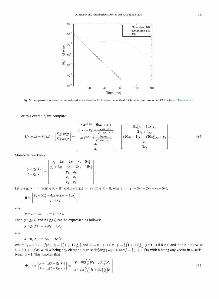
In addition, for Example 5.3, we also do comparisons among three neural networks based on FB function (considered in[20]), smoothed NR function (considered in this paper), and smoothed FB function (considered in [27]), respectively.Although Example 5.3 can be solved by all three neural networks, the neural network based on FB function does not behaveas good as the other two neural networks, see Fig. 5.

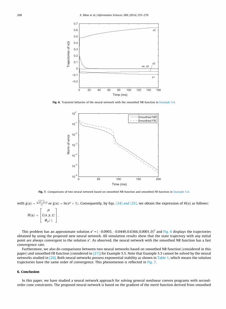
Example 5.4. Consider the following nonlinear second-order cone programming problem:

min f ðxÞ ¼ ex1x3 þ 3ðx1 þ x2Þ2 �ffiffiffiffiffiffiffiffiffiffiffiffiffiffiffiffiffiffiffiffiffiffiffiffiffiffiffiffiffiffiffiffi1þ ð2x2 � x3Þ2

qþ 1

2 x24 þ 1

2 x25

s:t: hðxÞ ¼ �24:51x1 þ 58x2 � 16:67x3 � x4 � 3x5 þ 11 ¼ 0

�g1ðxÞ ¼3x3

1 þ 2x2 � x3 þ 5x23

�5x31 þ 4x2 � 2x3 þ 10x3

3

x3

0B@

1CA 2 K3;

�g2ðxÞ ¼x4

3x5

� �2 K2:

0 5 10 15 20 25 30−0.2

−0.15

−0.1

−0.05

0

0.05

0.1

0.15

0.2

0.25

0.3

Time (ms)

Traj

ecto

ries

of x

(t)

x1

x2

x3

Fig. 4. Transient behavior of the neural network with the smoothed NR function in Example 5.3.

0 20 40 60 80 10010−6

10−5

10−4

10−3

10−2

10−1

100

Time (ms)

Nor

m o

f erro

r

Smoothed NRSmoothed FBFB

Fig. 5. Comparisons of three neural networks based on the FB function, smoothed NR function, and smoothed FB function in Example 5.3.

X. Miao et al. / Information Sciences 268 (2014) 255–270 267

For this example, we compute

Lðx; y; zÞ ¼ rf ðxÞ þrg1ðxÞyrg2ðxÞz

� �¼

x3eðx1x3Þ þ 6ðx1 þ x2Þ6ðx1 þ x2Þ þ 2ð2x2�x3Þffiffiffiffiffiffiffiffiffiffiffiffiffiffiffiffiffiffiffi

1þð2x2�x3Þ2p

x1eðx1x3Þ þ 2x2�x3ffiffiffiffiffiffiffiffiffiffiffiffiffiffiffiffiffiffiffi1þð2x2�x3Þ2p

x4

x5

2666666664

3777777775�

9x21y1 � 15x2

1y2

2y1 þ 4y2

ð10x3 � 1Þy1 þ ð30x23Þy2 þ y3

z1

3z2

26666664

37777775: ð24Þ

Moreover, we know

yþ g1ðxÞzþ g2ðxÞ

� �¼

y1 � 3x31 � 2x2 þ x3 � 5x2

3

y2 þ 5x31 � 4x2 þ 2x3 � 10x3

3

y3 � x3

z1 � x4

z2 � x5

26666664

37777775:

Let yþ g1ðxÞ :¼ ðu; �uÞ 2 R� R2 and zþ g2ðxÞ :¼ ðv ; �vÞ 2 R� R, where u ¼ y1 � 3x31 � 2x2 þ x3 � 5x2

3,

�u ¼ y2 þ 5x31 � 4x2 þ 2x3 � 10x3

3

y3 � x3

" #

and

v ¼ z1 � x4; �v ¼ z2 � x5:

Then, y + g1(x) and z + g2(x) can be expressed as follows:

yþ g1ðxÞ :¼ k1e1 þ k2e2

and

zþ g2ðxÞ :¼ j1f1 þ j2f2

where ki ¼ uþ ð�1Þik�uk; ei ¼ 12 1; ð�1Þi �u

k�uk

� �and ji ¼ v þ ð�1Þij�vj; f i ¼ 1

2 1; ð�1Þi �vj�v j

� �(i = 1,2) if �u – 0 and �v – 0, otherwise

ei ¼ 12 ð1; ð�1ÞiwÞ with w being any element in R2 satisfying kwk = 1, and fi ¼ 1

2 ð1; ð�1ÞitÞ with t being any vector in R satis-fying jtj = 1. This implies that

Ulð�Þ ¼y� Plðyþ g1ðxÞÞz� Plðzþ g2ðxÞÞ

� �¼

y� lg k1l

� �e1 þ lgðk2

l Þe2

z� lg j1l

� �f1 þ lg j2

l

� �f2

264

375 ð25Þ

0 20 40 60 80 100 120 140 160

−0.2

−0.1

0

0.1

0.2

0.3

0.4

0.5

0.6

0.7

Time (ms)

Traj

ecto

ries

of x

(t)

x1

x2

x3

x4, x5

Fig. 6. Transient behavior of the neural network with the smoothed NR function in Example 5.4.

0 50 100 150 20010−6

10−5

10−4

10−3

10−2

10−1

100

Time (ms)

Nor

m o

f erro

r

Smoothed NRSmoothed FB

Fig. 7. Comparisons of two neural network based on smoothed NR function and smoothed FB function in Example 5.4.

268 X. Miao et al. / Information Sciences 268 (2014) 255–270

with gðaÞ ¼ffiffiffiffiffiffiffiffia2þ4p

þa2 or gðaÞ ¼ lnðea þ 1Þ. Consequently, by Eqs. (24) and (25), we obtain the expression of H(u) as follows:

HðuÞ ¼l

Lðx; y; zÞUlð�Þ

264

375:

This problem has an approximate solution x⁄ = (�0.0903,�0.0449,0.6366,0.0001,0)T and Fig. 6 displays the trajectoriesobtained by using the proposed new neural network. All simulation results show that the state trajectory with any initialpoint are always convergent to the solution x⁄. As observed, the neural network with the smoothed NR function has a fastconvergence rate.

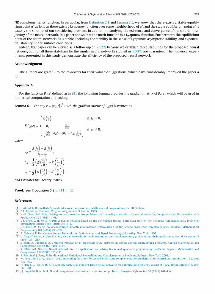
Furthermore, we also do comparisons between two neural networks based on smoothed NR function (considered in thispaper) and smoothed FB function (considered in [27]) for Example 5.5. Note that Example 5.5 cannot be solved by the neuralnetworks studied in [20]. Both neural networks possess exponential stability as shown in Table 1, which means the solutiontrajectories have the same order of convergence. This phenomenon is reflected in Fig. 7.

6. Conclusion

In this paper, we have studied a neural network approach for solving general nonlinear convex programs with second-order cone constraints. The proposed neural network is based on the gradient of the merit function derived from smoothed

X. Miao et al. / Information Sciences 268 (2014) 255–270 269

NR complementarity function. In particular, from Definition 2.1 and Lemma 2.3, we know that there exists a stable equilib-rium point u⁄ as long as there exists a Lyapunov function over some neighborhood of u⁄, and the stable equilibrium point u⁄ isexactly the solution of our considering problem. In addition to studying the existence and convergence of the solution tra-jectory of the neural network, this paper shows that the merit function is a Lyapunov function. Furthermore, the equilibriumpoint of the neural network (8) is stable, including the stability in the sense of Lyapunov, asymptotic stability, and exponen-tial stability under suitable conditions.

Indeed, this paper can be viewed as a follow-up of [20,27] because we establish three stabilities for the proposed neuralnetwork, but not all three stabilities for the similar neural networks studied in [20,27] are guaranteed. The numerical exper-iments presented in this study demonstrate the efficiency of the proposed neural network.

Acknowledgment

The authors are grateful to the reviewers for their valuable suggestions, which have considerably improved the paper alot.

Appendix A

For the function Pl(z) defined as in (5), the following Lemma provides the gradient matrix of Pl(z), which will be used innumerical computation and coding.

Lemma 6.1. For any z ¼ ðz1; zT2Þ

T 2 Rn, the gradient matrix of Pl(z) is written as

rPlðzÞ ¼

g0 z1l

� �I if z2 ¼ 0;

blclzT

2kz2k

clz2kz2k

alI þ ðbl � alÞz2zT

2

kz2k2

264

375 if z2 – 0;

8>>>><>>>>:

where

al ¼g k2

l

� �� g k1

l

� �k2l �

k1l

;

bl ¼12

g0k2

l

� �þ g0

k1

l

� �� �;

cl ¼12

g0k2

l

� �� g0

k1

l

� �� �;

and I denotes the identity matrix.

Proof. See Proposition 5.2 in [11]. h

References

[1] F. Alizadeh, D. Goldfarb, Second-order cone programming, Mathematical Programming 95 (2003) 3–52.[2] D.P. Bertsekas, Nonlinear Programming, Athena Scientific, 1995.[3] Y.-H. Chen, S.-C. Fang, Solving convex programming problems with equality constraints by neural networks, Computers and Mathematics with

Applications 36 (1998) 41–68.[4] J.-S. Chen, C.-H. Ko, S.-H. Pan, A neural network based on the generalized Fischer–Burmeister function for nonlinear complementarity problems,

Information Sciences 180 (2010) 697–711.[5] J.-S. Chen, P. Tseng, An unconstrained smooth minimization reformulation of the second-order cone complementarity problem, Mathematical

Programming 104 (2005) 293–327.[6] A. Cichocki, R. Unbehauen, Neural Networks for Optimization and Signal Processing, John wiley, New York, 1993.[7] C. Dang, Y. Leung, X. Gao, K. Chen, Neural networks for nonlinear and mixed complementarity problems and their applications, Neural Networks 17

(2004) 271–283.[8] S. Effati, A. Ghomashi, A.R. Nazemi, Application of projection neural network in solving convex programming problems, Applied Mathematics and

Computation 188 (2007) 1103–1114.[9] S. Effati, A.R. Nazemi, Neural network and its application for solving linear and quadratic programming problems, Applied Mathematics and

Computation 172 (2006) 305–331.[10] F. Facchinei, J. Pang, Finite-dimensional Variational Inequalities and Complementarity Problems, Springer, New York, 2003.[11] M. Fukushima, Z.-Q. Luo, P. Tseng, Smoothing functions for second-order-cone complementarity problems, SIAM Journal on Optimization 12 (2002)

436–460.[12] Q. Han, L.-Z. Liao, H. Qi, L. Qi, Stability analysis of gradient-based neural networks for optimization problems, Journal of Global Optimization 19 (2001)

363–381.[13] J.J. Hopfield, D.W. Tank, Neural computation of decision in optimization problems, Biological Cybernetics 52 (1985) 141–152.

270 X. Miao et al. / Information Sciences 268 (2014) 255–270

[14] X. Hu, J. Wang, A recurrent neural network for solving nonlinear convex programs subject to linear constraints, IEEE Transactions on Neural network16 (3) (2005) 379–386.

[15] X. Hu, J. Wang, A recurrent neural network for solving a class of general variational inequalities, IEEE Transactions on Systems, Man, and Cybernetics-B37 (2007) 528–539.

[16] S. Hayashi, N. Yamashita, M. Fukushima, A combined smoothing and regularization method for monotone second-order cone complementarityproblems, SIAM Journal on Optimization 15 (2005) 593–615.

[17] N. Kalouptisidis, Sigunal Processing Systems, Theory and Design, Wiley, New York, 1997.[18] C. Kanzow, I. Ferenczi, M. Fukushima, On the local convergence of semismooth Newton methods for linear and nonlinear second-order cone programs

without strict complementarity, SIAM Journal on Optimization 20 (2009) 297–320.[19] M.P. Kennedy, L.O. Chua, Neural network for nonlinear programming, IEEE Transactions on Circuits and Systems 35 (1988) 554–562.[20] C.-H. Ko, J.-S. Chen, C.-Y. Yang, Recurrent neural networks for solving second-order cone programs, Neurocomputing 74 (2011) 3646–3653.[21] L.-Z. Liao, H. Qi, L. Qi, Solving nonlinear complementarity problems with neural networks: a reformulation method approach, Journal of Computational

and Applied Mathematics 131 (2001) 342–359.[22] D.R. Liu, D. Wang, X. Yang, An iterative adaptive dynamic programming algorithm for optimal control of unknown discrete-time nonlinear systems

with constrained inputs, Information Sciences 220 (2013) 331–342.[23] O. Mancino, G. Stampacchia, Convex programming and variational inequalities, Journal of Optimization Theory and Applications 9 (1972) 3–23.[24] R.K. Miller, A.N. Michel, Ordinary Differential Equations, Academic Press, 1982.[25] S.-H. Pan, J.-S. Chen, A semismooth Newton method for the SOCCP based on a one-parametric class of SOC complementarity functions, Computational

Optimization and Applications 45 (2010) 59–88.[26] J.-S. Pang, L. Qi, Nonsmooth equation: motivation and algorithms, SIAM Journal on Optimization 3 (1993) 443–465.[27] J.-H. Sun, J.-S. Chen, C.-H. Ko, Neural networks for solving second-order cone constrained variational inequality problem, Computational Optimization

and Applications 51 (2012) 623–648.[28] D.W. Tank, J.J. Hopfield, Simple neural optimization network: an A/D converter, signal decision circuit, and a linear programming circuit, IEEE

Transactions on Circuits and Systems 33 (1986) 533–541.[29] S.J. Wright, An infeasible-interior-point algorithm for linear complementarity problems, Mathematical Programming 67 (1994) 29–51.[30] A.L. Wu, S.P. Wen, Z.G. Zeng, Synchronization control of a class of memristor-based recurrent neural networks, Information Sciences 183 (2012) 106–

116.[31] Y. Xia, H. Leung, J. Wang, A projection neural network and its application to constrained optimization problems, IEEE Transactions on Circuits and

Systems-I 49 (2002) 447–458.[32] Y. Xia, H. Leung, J. Wang, A general projection neural network for solving monotone variational inequalities and related optimization problems, IEEE

Transactions on Neural Networks 15 (2004) 318–328.[33] Y. Xia, J. Wang, A recurrent neural network for solving nonlinear convex programs subject to linear constraints, IEEE Transactions on Neural Networks

16 (2005) 379–386.[34] M. Yashtini, A. Malek, Solving complementarity and variational inequalities problems using neural networks, Applied Mathematics and Computation

190 (2007) 216–230.[35] J. Zabczyk, Mathematical Control Theorem: An Introduction, Birkhäuser, Boston, 1992.[36] G.D. Zhang, Y. Shen, Q. Yin, J.W. Sun, Global exponential periodicity and stability of a class of memristor-based recurrent neural networks with multiple

delays, Information Sciences 232 (2013) 386–396.