A Simulation Study of a Parametric Mixture Model of Three Different Distributions to Analyze Heterogeneous Survival Data

Modern Applied Science; Vol. 7, No. 7; 2013 ISSN 1913-1844 E-ISSN 1913-1852

Published by Canadian Center of Science and Education

1

A Simulation Study of a Parametric Mixture Model of Three Different Distributions to Anlayze Heterogeneous Survival Data

Yusuf Abbakar Mohammed1,2, Bidin Yatim1 & Suzilah Ismail1

1 School of Quantitative Sciences, College of Arts and Sciences, Universiti Utara Malaysia, Malaysia 2 Dept. of Mathematics and Statistics, Faculty of Sciences, University of Maiduguri, Nigeria

Correspondence: Yusuf Abbakar Mohammed, 17, 2D, Sisiran Universiti Utara Malaysia, Sintok, Kedah, Malaysia. Tel: 60-1-463-7205. E-mail: [email protected]

Received: April 7, 2013 Accepted: May 27, 2013 Online Published: June 6, 2013

doi:10.5539/mas.v7n7p1 URL: http://dx.doi.org/10.5539/mas.v7n7p1

Abstract

In this paper a simulation study of a parametric mixture model of three different distributions is considered to model heterogeneous survival data. Some properties of the proposed parametric mixture of Exponential, Gamma and Weibull are investigated. The Expectation Maximization Algorithm (EM) is implemented to estimate the maximum likelihood estimators of three different postulated parametric mixture model parameters. The simulations are performed by simulating data sampled from a population of three component parametric mixture of three different distributions, and the simulations are repeated 10, 30, 50, 100 and 500 times to investigate the consistency and stability of the EM scheme. The EM Algorithm scheme developed is able to estimate the parameters of the mixture which are very close to the parameters of the postulated model. The repetitions of the simulation give parameters closer and closer to the postulated models, as the number of repetitions increases, with relatively small standard errors.

Keywords: survival time analysis, maximum likelihood, em-algorithm, mixture model, simulation, exponential distribution, gamma distribution, weibull distribution

1. Introduction

The survival time data analysis is concerned with the analysis of time to occurrence of a particular event of interest. The data are usually related to clinical studies of human or laboratory studies of animal or studies to test the life time of some devices. Historically, nonparametric techniques were used to handle survival data. Parametric distributions are the conventional techniques in statistics; they are very useful if the selected parametric probability distribution fits the data properly. The most frequently used parametric distributions in survival time data analysis includes the Exponential, Gamma, and Weibull among others (Ibrahim, Chen, & Sinha, 2001; Kalbfleisch & Prentice, 2002; Lawless, 2003; Lee & Wang, 2003). In cases of data with heterogeneous structure, mixture distributions are more convenient to handle such data. Recently, a considerable number of authors used mixture model technique to analyse survival time data. Cheng and Fu (1982) proposed a parametric mixture model of Weibull distribution where they employed the weighted least squares method to estimate the parameters. Jiang and Kececioglu (1992a) estimated the parameters of a mixture model of Weibull distribution using graphical approach. They (Jiang & Kececioglu, 1992b) also developed a new procedure to estimate the parameters of a mixture model of Weibull.

Zhang (2008) proposed a two-component mixture model of the Weibull-Weibull distribution to model survival time data and investigated the suitability of the model in survival analysis. Also Erisoglu, Erisoglu and Erol (2012) modelled heterogeneous survival time data by a mixture model of Gamma-Gamma, a mixture of Lognormal-Lognormal and a mixture of the Weibull- Weibull distributions, where they investigated the best fit model to real survival time data. A mixture model of mixed distributions was proposed by Ersioglu and Erol (2010), to model heterogeneous survival time data, where they employed a two component mixture model of the Extended Exponential-Geometric (EEG) distribution. In Erisoglu, Erisoglu and Erol (2011), a mixture of two different distributions Exponential-Gamma, Exponential-Weibull and Gamma-Weibull were used to model heterogeneous survival data.

www.ccsenet.org/mas Modern Applied Science Vol. 7, No. 7; 2013

2

In the case of open-heart surgery, Blackstone, Naftel and Turner Jr. (1986) identified three overlapping phases of death after surgery which could be modelled by a three component parametric mixture model instead of the conventional parametric survival time model, as was pointed out by Ng, Mclachan, Yau, and Lee (2004) and Philips, Coldman, and McBride (2002). Mixture of different distributions would be appropriate to model a different mode of hazard in heterogeneous survival time data. The Expectation Maximization Algorithm (EM) is effectively used in cases of data with missing of unobserved observations (Dempster, Laird, & Rubin, 1977). The maximum likelihood estimates of the parameters of the survival mixture model are estimated usually via (EM) (Mclachlan & Peel, 2000; Mclachlan & Krishnan, 2008).

The purpose of this paper is to investigate the consistency and stability of EM in estimating the parameters and the appropriateness of a mixture of three different distributions in analysing heterogeneous survival time data. The article is arranged as follows. Section two to discusses survival analysis and some frequently used theoretical distributions and their properties. Section three will be devoted to discussing the mixture model of three different distributions in the survival time analysis. Section four for the implementation of EM scheme to estimate the maximum likelihood estimator of the model. Section five is devoted to simulation, estimation of the parameters of the model and demonstrates the successful convergence of the EM, consistency and stability of the scheme.

2. Survival Analysis and Functions

Survival analysis deals with the implementation of certain statistical techniques to model and analyze survival time data. The primary interest in such data is the endpoint time when an event of interest occurs. Generally, the events of interest are referred to as failures. They could be; the time to death of a patient, time to learning a new skill, time to exit from unemployment, time to promotion for employees and time to breakdown of some device. The response of primary interest, T is a non-negative random variable representing survival time of an individual and can be described by three important functions. The probability density function (pdf) denoted by ( )f t , which can be written as

( )dF tf t

dt (1)

Where ( )F t is the the responsetion function of response variable T. The probability density function can also be presented graphically, the graph of ( )f t , is known as the density curve. The density function ( )f t is a nonnegative function and the area between the curve and the t axis is equal to 1. The survival function denoted by ( )S t , which can be written as

1S t F x (2)

that represents the probability that an individual survives beyond time . Note that the survival function is a monotonic decreasing continuous function with 0 1S and lim 0

tS S t

. The hazard function which

is denoted by ( )h t , and can be written as

0

( | ) ( )lim

( )t

p t T t t T t f th t

t s t

(3)

representing the probability that an individual fails within a small interval ( , Δ )t t t , given that the individual survived to the beginning of the interval. The cumulative hazard function of the survival time T is defined by;

0

t

H t h u du (4)

Therefore, when 0t then 1S t and 0H t , and when t then, 0S t and H t . That is, the cumulative hazard function can assume any value between zero to infinity. The hazard function specifies the instantaneous rate of failure at time given that the individual survived up to time , and sometimes it is known as the instantaneous failure rate, force of mortality, conditional mortality rate, and age-specific failure rate. The hazard function is also presented graphically. These three functions are equivalent if any one of them is known then the two others can be derived (Lee & Wang, 2003).

Parametric statistical techniques are convenient tools in survival analysis; provided that the selected parametric distribution adequately fit the data at hand. In the literature the Exponential, Gamma and Weibull probability distributions are the most frequently used density functions in modelling survival time data (Cheng & Fu, 1982; Jian & Kececioglu, 1992a; Ng, Mclachan, Yau, & Lee, 2004; Zhang, 2008; Erisoglu & Erol, 2010; Erisoglu,

www.ccsenet.org/mas Modern Applied Science Vol. 7, No. 7; 2013

3

Erisoglu, & Erol, 2011, 2012). The probability density function ( )f t , survival functions ( )S t and hazard functions ( )h t of these distributions are highlighted below.

Exponential Distribution

, 0tExpf t e t (5)

tExpS t e (6)

1ExpE t

(7)

Gamma Distribution

1 , 0Γ( )

t

Gm

ef t t t and

(8)

xΓ (α)1

Γ( )GmS t

(9)

GmE (10)

where Γ ( )x is known as the incomplete Gamma function.

Weibull Distribution

1

, 0Wbl

t tf t exp t and

(11)

Wbl

tS t exp

(12)

1Γ 1WblE t

(13)

3. Parametric Mixture of Three Different Distributions

Mixture models are implemented to analyse survival time data in different situations, because of their flexibility, and they are the best choice in situations where a single parametric distribution may not suffice (Mclachlan & Peel, 2000; Fruhwirth-Schnatter, 2006). A mixture model of three different distributions is considered where it is assumed that it is sampled from a population consisting of three subpopulation or subgroups. The mixture model can be expressed as

, , 1 2 3;Θ ( ; ) ( ; ) ( ; )X Y Q X X Y Y Q Qf t f t f t f t (14)

Where the vector 1 2 3Θ ( , , , , , )X Y Q , contains all the unknown parameters in the mixture model. The functions ; , ( ; )X X Y Yf t f t and ( ; )Q Qf t are known as the mixture component density functions for some parameters ,X Y and Q respectively.

In this paper a mixture of three different distributions of Exponential, Gamma and Weibull is proposed to model heterogeneous survival time data, the different distribution takes care of different hazard mode in the heterogeneous data, and the model defined as

1 2 1 1 3 2 2;Θ ( ; ) ( ; , ) ( ; , )Exp Gm Wbl Exp Gm Wblf t f t f t f t (15)

Where 'i s are the mixing proportions or mixing probabilities and3

1

1ii

. The functions Expf , Gmf and Wblf ,

as defined in (5), (8) and (11), are the probability density functions of Exponential, Gamma and Weibull distributions respectively.

4. The Expectation Maximization Algorithm (EM) and Parameter Estimation

The EM Algorithm is frequently employed in the literature as an efficient technique to estimate the maximum likelihood estimators of finite mixture models (Mclachlan & Krishnan, 2008).

Let 1 2, , , nt t t be a set of observations of n incomplete data and 1 2 3, ,z z z be a set of missing observations, where 1ki k iz z t , if the observation belongs to the kth component and 0 otherwise for 1,2,3k and

1, ,i n . Here z`s are treated as missing values when applying the EM Algorithm to the mixture distribution.

www.ccsenet.org/mas Modern Applied Science Vol. 7, No. 7; 2013

4

The EM Algorithm proceeds in two steps, the Expectation step or the E-step and Maximization step or the M-step.

In the E step the iz Variables are considered as missing data, the expectation ,( | )ki iE z t is obtained to estimate the hidden variable vector 1 2 3, ][ ,i i i iz z z z .

Thus

1

1 11 2 3

( ; )|

; ; ( ; )ˆ X i X

i i iX i X Y i Y Q i Q

f tz E z t

f t f t f t

(16)

2

2 21 2 3

( ; )|

; ; ( ; )ˆ Y i Y

i i iX i X Y i Y Q i Q

f tz E z t

f t f t f t

(17)

3

3 31 2 3

( ; )|

; ; ( ; )ˆ Q i Q

i i iX i X Y i Y Q i Q

f tz E z t

f t f t f t

(18)

The functions 1 2| , |i i i iE z t E z t and 3 |i iE z t calculated in the E step will be maximized in the M step of the

EM Algorithm under the condition3

1

1ii

. The Lagrange method can be employed to estimate the mixing

probabilities and parameter vector [ , , ]X Y Q . The estimated mixing probabilities are;

1 11

ˆ ˆ1 n

ii

zn

(19)

2 21

ˆ ˆ1 n

ii

zn

(20)

3 31

ˆ ˆ1 n

ii

zn

(21)

The maximum likelihood estimator of the parameter for the proposed model can be obtained by the equation (22)

1

1 11 1

ˆ ˆ ˆn n

i i ii i

z t z

(22)

The maximum likelihood estimators of the parameters and for the proposed model can be estimated from the equations (23) and (24) respectively

n n

2i i 2i it 1 t 11, 1, n n

2i 2it 1 t 11,( 1) 1,

'1,

1,

ˆ ˆˆ ˆ

ˆ

z t z ln tln( ) Ψ ln

ˆˆ ˆ

ˆ

z

1ˆ

z

Ψ

r r

r r

rr

(23)

and 1

1 1 2 21 1

ˆ ˆ ˆ ˆn n

i i ii i

z z t

(24)

Where is the number of Newton-Raphson iteration within EM Algorithm and Ψ . and Ψ′ . are a digamma and trigamma functions respectively.

The maximum likelihood estimators of the parameters and for the proposed model can be estimated from the equations (25) and (26) respectively.

2,

2,( 1) 2, 2

2 22,

ˆˆ ˆ

1ˆ

1 rr

r r

r r

r r r

r r

CA

B

B D C

B

(25)

www.ccsenet.org/mas Modern Applied Science Vol. 7, No. 7; 2013

5

Where1

3 31 1

ˆ ˆ lnn n

r i i ii i

A z z t

, 2,ˆ

31

ˆ r

n

r i ii

B z t

, 2,

31

ˆˆ lnr

n

r i i ii

C z t t

, 2, 2ˆ

31

ˆ lnr

n

r i i ii

D z t t

and r is the number

of Newton-Raphson iteration within EM Algorithm.

2

2

11

2 3 31 1

ˆˆˆ ˆ ˆ

n n

i i ii i

z z t

(26)

5. Simulation

Simulations were performed to investigate the convergence of the proposed EM scheme. Samples of size 400 observations were generated, each of them randomly sampled from three-component survival mixture model of Exponential, Gamma and Weibull. There was no restriction imposed on the number of iterations and convergence was achieved when the differences between successive estimates were less than 10-4. Three different postulated models were considered with a different set of parameters. The result of the parameter estimation of the three sets of mixture model is given below:

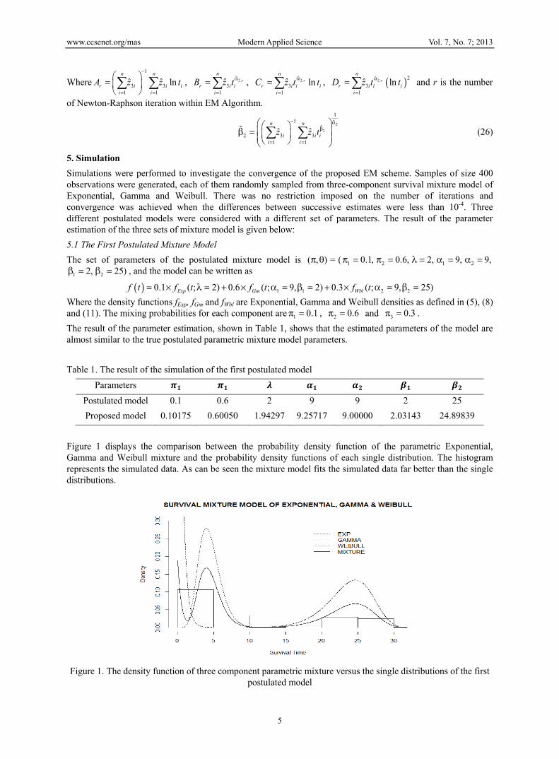
5.1 The First Postulated Mixture Model

The set of parameters of the postulated mixture model is 1 2 1 20.1, 0.6( , ) = ( 2, 9,, 9, 1 22, 25) , and the model can be written as

1 1 2 20.1 ( ; 2) 0.6 ( ; 9, 2) 0.3 ( ; 9, 25)Exp Gm Wblf t f t f t f t

Where the density functions fExp, fGm and fWbl are Exponential, Gamma and Weibull densities as defined in (5), (8) and (11). The mixing probabilities for each component are 1 0.1 , 2 0.6 and 3 0.3 .

The result of the parameter estimation, shown in Table 1, shows that the estimated parameters of the model are almost similar to the true postulated parametric mixture model parameters.

Table 1. The result of the simulation of the first postulated model

Parameters

Postulated model 0.1 0.6 2 9 9 2 25

Proposed model 0.10175 0.60050 1.94297 9.25717 9.00000 2.03143 24.89839

Figure 1 displays the comparison between the probability density function of the parametric Exponential, Gamma and Weibull mixture and the probability density functions of each single distribution. The histogram represents the simulated data. As can be seen the mixture model fits the simulated data far better than the single distributions.

Figure 1. The density function of three component parametric mixture versus the single distributions of the first

postulated model

www.ccsenet.org/mas Modern Applied Science Vol. 7, No. 7; 2013

6

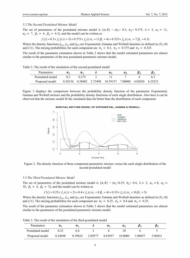
5.2 The Second Postulated Mixture Model

The set of parameters of the postulated mixture model is , = ( = 0.3, = 0.375, 3, 11, 7, 4, 6.3), and the model can be written as

1 1 2 20.3 ( ; 3) 0.375 ( ; 11, 4) 0.325 ( ; 7, 6.3)E G Wf t f t f t f t

Where the density functions fExp, fGm and fWbl are Exponential, Gamma and Weibull densities as defined in (5), (8) and (11). The mixing probabilities for each component are 0.3, 0.375 and 0.325.

The result of the parameter estimation shown in Table 2 shows that the model estimated parameters are almost similar to the parameters of the true postulated parametric mixture model.

Table 2. The result of the simulation of the second postulated model

Parameters

Postulated model 0.3 0.375 3 11 7 4 6.3

Proposed model 0.30154 0.38002 2.72490 10.39157 7.00000 4.02030 6.25523

Figure 2 displays the comparison between the probability density function of the parametric Exponential, Gamma and Weibull mixture and the probability density functions of each single distribution. Also here it can be observed that the mixture model fit the simulated data far better than the distribution of each component.

Figure 2. The density function of three component parametric mixture versus the each single distribution of the

second postulated model

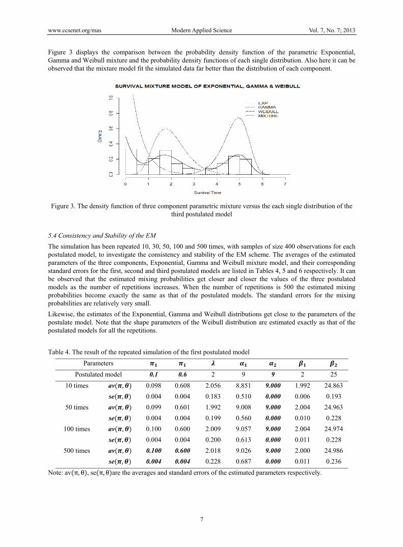
5.3 The Third Postulated Mixture Model

The set of parameters of the postulated mixture model is , = ( =0.25, = 0.4, 2, 8, 10, 4, 5), and the model can be written as

1 1 2 20.25 ( ; 2) 0.4 ( ; 8, 4) 0.35 ( ; 10, 5)E G Wf t f t f t f t

Where the density functions fExp, fGm and fWbl are Exponential, Gamma and Weibull densities as defined in (5), (8) and (11). The mixing probabilities for each component are 0.25, 0.4 and 0.35.

The result of the parameter estimation shown in Table 3 shows that the model estimated parameters are almost similar to the parameters of the postulated parametric mixture model.

Table 3. The result of the simulation of the third postulated model

Parameters

Postulated model 0.25 0.4 2 8 10 4 5

Proposed model 0.24698 0.39824 2.09577 8.03957 10.0000 3.98857 5.00431

www.ccsenet.org/mas Modern Applied Science Vol. 7, No. 7; 2013

7

Figure 3 displays the comparison between the probability density function of the parametric Exponential, Gamma and Weibull mixture and the probability density functions of each single distribution. Also here it can be observed that the mixture model fit the simulated data far better than the distribution of each component.

Figure 3. The density function of three component parametric mixture versus the each single distribution of the

third postulated model

5.4 Consistency and Stability of the EM

The simulation has been repeated 10, 30, 50, 100 and 500 times, with samples of size 400 observations for each postulated model, to investigate the consistency and stability of the EM scheme. The averages of the estimated parameters of the three components, Exponential, Gamma and Weibull mixture model, and their corresponding standard errors for the first, second and third postulated models are listed in Tables 4, 5 and 6 respectively. It can be observed that the estimated mixing probabilities get closer and closer the values of the three postulated models as the number of repetitions increases. When the number of repetitions is 500 the estimated mixing probabilities become exactly the same as that of the postulated models. The standard errors for the mixing probabilities are relatively very small.

Likewise, the estimates of the Exponential, Gamma and Weibull distributions get close to the parameters of the postulate model. Note that the shape parameters of the Weibull distribution are estimated exactly as that of the postulated models for all the repetitions.

Table 4. The result of the repeated simulation of the first postulated model

Parameters Postulated model 0.1 0.6 2 9 9 2 25

10 times av , 0.098 0.608 2.056 8.851 9.000 1.992 24.863

se , 0.004 0.004 0.183 0.510 0.000 0.006 0.193

50 times av , 0.099 0.601 1.992 9.008 9.000 2.004 24.963

se , 0.004 0.004 0.199 0.560 0.000 0.010 0.228

100 times av , 0.100 0.600 2.009 9.057 9.000 2.004 24.974

se , 0.004 0.004 0.200 0.613 0.000 0.011 0.228

500 times av , 0.100 0.600 2.018 9.026 9.000 2.000 24.986

se , 0.004 0.004 0.228 0.687 0.000 0.011 0.236

Note: av π, θ , se π, θ are the averages and standard errors of the estimated parameters respectively.

www.ccsenet.org/mas Modern Applied Science Vol. 7, No. 7; 2013

8

Table 5. The result of the simulation of the second postulated model

Parameters

Postulated model 0.3 0.375 3 11 7 4 6.3

10 times

av , 0.299 0.375 2.963 10.746 7.000 4.011 6.291

se , 0.004 0.007 0.225 0.863 0.000 0.004 0.059

50 times

av , 0.301 0.372 3.014 10.845 7.000 3.993 6.277

se , 0.004 0.009 0.231 0.866 0.000 0.005 0.082

100 times

av , 0.301 0.375 3.016 10.920 7.000 4.004 6.298

se , 0.005 0.009 0.214 0.775 0.000 0.005 0.074

500 times

av , 0.300 0.375 3.018 11.053 7.000 3.997 6.291

se , 0.005 0.009 0.223 0.848 0.000 0.005 0.076

Note: av π, θ , se π, θ are the averages and standard errors of the estimated parameters respectively.

Table 6. The result of the repeated simulation of the third postulated model

Parameters

Postulated model 0.25 0.4 2 8 10 4 5

10 times av , 0.249 0.399 2.007 7.978 10.000 3.999 5.022

se , 0.009 0.007 0.098 0.475 0.000 0.004 0.025

50 times av , 0.251 0.399 1.990 7.951 10.000 4.012 4.996

se , 0.010 0.010 0.096 0.491 0.000 0.005 0.038

100 times av , 0.250 0.400 2.005 8.028 10.000 4.004 5.000

se , 0.010 0.099 0.105 0.529 0.000 0.005 0.041

500 times av , 0.250 0.400 2.001 8.014 10.000 3.999 5.001

se , 0.009 0.010 0.103 0.494 0.000 0.005 0.041

Note: av π, θ , se π, θ are the averages and standard errors of the estimated parameters respectively.

The table’s show that the EM scheme converged to the true values of the parameter in 10, 50, 100 and 500 repetitions and that emphasizes the stability of the algorithm in estimating the parameters with different proportion of mixing probabilities. The averages are close to the true values of the parameters and the standard errors are relatively small which suggest that the EM parameter estimates performed consistently.

6. Conclusions

The paper proposed a mixture model of three different distributions namely, Exponential, Gamma and Weibull to model the heterogeneous survival time data. EM algorithm was employed to estimate the maximum likelihood estimator of the parameter of the parametric mixture model. The convergence of the EM was investigated through the simulations performed. The results revealed that the EM successfully estimated the parameters of the three component mixture model. The mixture model of three different distributions, Exponential, Gamma and Weibull could be successfully applied to model heterogeneous survival time data instead of the conventional parametric models.

References

Blackstone, E. H., Naftel, D. C., & Turner Jr., M. E. (1986). The decomposition of time-varying hazard into phases, each incorporating a separate stream of concomitant information. Journal of the American Statistical Association, 81(395), 615-624. http://dx.doi.org/10.1080/01621459.1986.10478314

Cheng, S. W., & Fu, J. C. (1982). Estimation of mixed Weibull parameters in life testing. Reliability, IEEE Transactions on, R-31(4), 377-381. http://dx.doi.org/10.1109/TR.1982.5221382

www.ccsenet.org/mas Modern Applied Science Vol. 7, No. 7; 2013

9

Dempster, A. P., Laird, N. M., & Rubin, D. B. (1977). Maximum likelihood estimation from incomplete data via the EM algorithm (with discussion)”. Journal of Royal Statistical Society. Series B, 39, 1-38.

Erişoğlu, Ü., Erişoğlu, M., & Erol, H. (2011). A mixture model of two different distributions approach to the analysis of heterogeneous survival data. International Journal of Computational and Mathematical Sciences, 5(2).

Erişoğlu, Ü., Erişoğlu, M., & Erol, H. (2012). Mixture model approach to the analysis of heterogeneous survival time data. Pakistan Journal of Statistics, 28(1), 115-130.

Erişoğlu, Ü., & Erol, H. (2010). Modelling heterogeneous survival data using mixture of extended exponential-geometric distributions. Communications in Statistics - Simulation and Computation, 39(10), 1939-1952. http://dx.doi.org/10.1080/03610918.2010.524335

Fruhwirth-Schnatter, S. (2006). Finite mixture and markovs switching models: Springer.

Ibrahim, J. G., Chen, M. H., & Sinha, D. (2001). Bayesian survival analysis. New York: Springer-verlag. http://dx.doi.org/10.1007/978-1-4757-3447-8

Jiang, S., & Kececioglu, D. (1992a). Graphical representation of two mixed-Weibull distributions. IEEE Transaction on Reliability, 41, 241-247. http://dx.doi.org/10.1109/24.257789

Jiang, S., & Kececioglu, D. (1992b). Maximum likelihood estimates, from censored data, for mixed-Weibull distributions. IEEE Transaction on Reliability, 41, 248-255. http://dx.doi.org/10.1109/24.257791

Kalbfleisch, J. D., & Prentice, R. L. (2002). The statistical analysis of failure time data (2nd ed.). Hoboken, New Jersey: John Wiley & Sons, Inc. http://dx.doi.org/10.1002/9781118032985

Lawless, J. F. (2003). Statistical models and methods of lifetime data (2nd ed.). Hoboken, New Jersey: John Wiley and Sons, Inc.

Lee, E. T., & Wang, J. W. (2003). Statistical methods for survival time data analysis (3rd ed.). John Wiley & son.

McLachlan, G. J., & Peel, D. (2000). Finite mixture models. John Wiley & Sons, Inc. http://dx.doi.org/10.1002/0471721182

McLachlan, G. J., & Krishnan, T. (2008). The EM algorithm and extensions (2nd ed.). Hoboken, New Jersey: John Wiley & Sons, Inc. http://dx.doi.org/10.1002/9780470191613

Ng, A. S. K., McLachlan, G. J., Yau, K. K. W., & Lee, A. H. (2004). Modelling the distribution of ischaemic stroke-specific survival time using an EM-based mixture approach with random effects adjustment. Statistics in Medicine, 23(17), 2729-2744. http://dx.doi.org/10.1002/sim.1840

Phillips, N., Coldman, A., & McBride, M. L. (2002). Estimating cancer prevalence using mixture models for cancer survival. Statistics in Medicine, 21(9), 1257-1270. http://dx.doi.org/10.1002/sim.1101

Sun, J. (2006). The statistical analysis of interval-cencored failure time data. New York: Springer Science, Business Media.

Zhang, Y. (2008). Parametric mixture models in survival analysis with application, (Doctoral Dissertation) UMI Number: 3300387, Graduate School, Temple University.

Note

All computations are performed with the R language version 2.14.1 (2011 -12-22). http://CRAN.R-project.org

Copyrights Copyright for this article is retained by the author(s), with first publication rights granted to the journal.

This is an open-access article distributed under the terms and conditions of the Creative Commons Attribution license (http://creativecommons.org/licenses/by/3.0/).