A Simulation Analysis of the Relationship between Retail Sales and Shopping Center Rents

Marquette Universitye-Publications@Marquette

Finance Faculty Research and Publications Finance, Department of

5-1-2001

A Simulation Analysis of the Relationship betweenRetail Sales and Shopping Center RentsGregory H. ChunUniversity of Wisconsin - Madison

Mark EppliMarquette University, [email protected]

James D. ShillingUniversity of Wisconsin - Madison

Published version. Journal of Real Estate Research, Vol. 21, No. 3 (May/June 2001): 163-186.Publisher Link. © 2001 American Real Estate Society. Used with permission.Mark Eppli was affiliated with George Washington University at the time of publication.

https://epublications.marquette.edu

https://epublications.marquette.edu/fin_fac

https://epublications.marquette.edu/fin

http://aresjournals.org/doi/abs/10.5555/rees.21.3.b0415617172ju3g5

A Simulation Analysis

between Retail Sales and

of the Relationship

Shopping

Center Rents

Authors

Abstract

Introduction

Gregory H. Chun, Mark J. Eppli and

James D. Shilling

This article examines the variation in rents per square foot among regional shopping centers in the United States in response to variation in retail sales per square foot. The analysis breaks new ground by treating base and percentage rents as endogenous functions of retail sales. The analysis further distinguishes between de facto, if not de jure, fixed and percentage leases, and between new versus existing leases. Simulation results suggest that shopping center rents can easily increase in the short-run as retail sales decrease, or they can easily decrease as retail sales increase. In addition, the results suggest that shopping center rents per square foot generally react more aggressively to an increase in retail sales per square foot over time than to a decrease in retail sales per square foot, all else equal.

This article is concerned with the effects of variations in retail sales on the time path of shopping center rents. On the basis of a variety of evidence, including a recent article by Wheaton and Torto (1995), the case for examining the relationship between retail sales and shopping center rents is compelling. 1 Between 1968 and 1993, for example, retail sales in regional shopping centers in the United States (in constant dollars per square foot) fell by 20% to 40%, while rents per square foot (constant dollars) almost doubled. Since then shopping center rent and retail sales changes, for many retailers, have been such that rents and retail sales are now, as it were, just in balance. For other retailers, changes in shopping center rents have continued to outpace changes in retail sales. Still for other retailers, the changes in shopping center rent and retail sales would appear to be on the "yellow brick road" leading back to an eqUilibrium level (see Exhibits 1-10).

As an explanation for some of these trends-particularly, the tendency for changes in shopping center rents to deviate noticeably from changes in retail sales in the short-run-this article develops a theoretical model of shopping center rents, with

J R E R v 0 I. 2 1 No.3-2001

164 Chun, Eppli and Shilling

Exh I b It 1 I Rents vs. Sales Per Square Foot: Specialty Foods 11961 = 100)

1200~------------------------------------------------

1000+-------------------------------------------~r_ ~ 800+-__________________________________ ~R~~+t~~.~~ c:I L:::{L ~ 600+---------------------------------------~--~~-----.: /-,,~'

400+-------------------------------~~~~--~_T------.~~ Sales

200~==~==~==~~==~--=---------~~---0+---.--.---.--.---.--.---.--.---.--.---.--.---.--.

N

" 0\ -Year

-ex: 0\ -

numerical parameters. The objectives of the article are to describe the model and to present a variety of simulations results based on it.

The particular model specified here and the simulation results obtained relate wholly to regional shopping centers in the U.S. The model has several antecedents in the literature (Benjamin, Boyle and Sirmans, 1992; Brueckner, 1993; and Miceli and Sirmans, 1995). However, it breaks new ground by (1) treating base and percentage rents as endogenous functions of retail sales; (2) distinguishing between de facto, if not de jure, fixed and percentage leases; and (3) relaxing

900 800

700

600 ~ 500 ~

.: 400 300

200 100

o

Ex h I b It 2 I Rents vs. Soles Per Square Foot: ladies Specialty Wear (1961 = 100)

-\C 0\ -

\C \C 0\ -~-

ex: " 0\ -

Year

,.,--

-00 0\ ....

R~ntL

/ -......-

/ Ii"'" /L Sales /~

o 0\ 0\ - " 0\

0\ -

Retail Sales and Shopping Center Rents 165

Ex h I bit 3 I Rents vs. Sales Per Square Foot: ladies Wear 11961 = 100)

600.------------------------------------------------~

500+----------------------------------DruKI~~lt~~--~~~------

400+---------------------------------~7'--------------

! ~ 300 +-____________________________ ~c~~-"~=----'"l't"='---r.:::_---.5 ~ Sales

200+-----------_______ -----=~~~--------------------

100+---------~~---------------------------------

O+--r--.--.-.--.-~r-_.-_.-._-._-.--.-_.__.

.... \C C'\ ....

\C \C C'\ ....

N ...... C'\ ....

00 ...... C'\ -

Year

.... 00 C'\ ....

~ C'\ -

...... 00 C'\ -

o ~ - ~

C'\

II)

~ - ....

assumptions regarding lagged effects. The model is also unique in that it is estimated completely with cross-section data. The model is used to generate a set of ex post forecasts over time. Our major findings are:

1. There is not a direct proportionality between changes in retail sales and shopping center rents, at least not in most cases and particularly not in the short-run. In the short-run, shopping center rents can easily increase as retail sales decrease, or they can easily decrease as retail sales increase.

2. The analysis here suggests that a given percentage increase in retail sales per square foot raises rents per square foot over time, all else equal, with the rent increases in the short-run being greater for shopping centers

1200

1000

~ 800

II)

"C 600 c - 400

200

0

Exhibit 4 I Rents vs. Sales Per Square Foot: Children's Wear 11961 = 100)

-\C C'\ ....

\C \C C'\ ....

C'\ \C C'\ ....

N ...... C'\ ....

II) ...... C'\ ....

Year

J R E R

.... 00 C'\ ....

Vo I. 2 1

c::: 0\ 0', -

Rent /

II') C'\ C'\ ....

...... C'\ C'\ ....

No.3-2001


Exh I b It 5 I Rents vs. Sales Per Square Foot: Men's Wear (1961 = 100)

600

500

400 ~

Rent ~ -41

] 300 ~.,. Sales -200

100 -0 ....

\0 0\ ....

I"l \0 \0 \0 0\ 0\ .... ....

Year

-00 0\ -

experiencing nsmg retail sales per square foot than for centers experiencing constant (or declining) retail sales per square foot.

3. In the long run, shopping center rents per square foot generally react more aggressively to an increase in retail sales per square foot over time than to a decrease in retail sales per square foot, all else equal.

These conclusions are, of course, subject to several limitations. First, the theory underlying the analysis deals with rents per square foot and retail sales per square foot for individual stores over time, yet the variables we measure are at a point in time (except for retail sales per square foot) and apply to aggregate data. Second, we use cross-sectional data to make inferences about how rents per square

Ex hI bIt 6 I Rents vs. Sales Per Square Foot: Family Apparel (1961 = 100)

1000.-------------------------------------------------800+-__________________________________ ~R~en~t~--7----~----

~ ~ 600+-----------------------------------/--~----~--------

] 400+---------------------------------~~~~-~~~-~~-------~------~ Sales

200+-------------~~--=~----=---------------------

----------------~ .. ~ 0+---.--.---.---.--.---.---.--.---.---.--.---.---.--. .... I"l 1.0 0\ N trl 00 .... ~ ~ 0 I"l trl ~

\0 \0 1.0 1.0 ~ ~ ~ 00 ex:: ex:: 0\ 0\ 0\ 0\ 0\ 0\ 0\ 0\ 0\ 0\ 0\ 0\ 0\ 0\ 0\ 0\ 0\ 0\ - .... .... .... - .... .... .... .... .... .... .... -

Year · ... ·M. ~ r, • '~'_"


Exhibit 7 I Rents vs. Sales Per Square Foot; Family Shoes 11961 = 1001

600~-----------------------------------------------

Rent / 500+-----------------------~~lr~~~------

400+-------------------------~~===~--~~J~~--~ ~. ~ ~;'es ]300+--------------------~--~~~--~~-~~--~~=---

200+-------------------~~~~----------------------

100+-----~~~~~~~-----------------------------O+---r_~--_r--~--~~r_~--_.--,_--.__.--_.--_.__. -\C

a.. -N r-a.. - oe r-

a.. -Year

-oe a.. -

foot would change from one equilibrium at a point in time to another eqUilibrium at a later point in time. This use depends on the assumption that the cross-sectional observations themselves represent equilibria. Third, to the extent that the estimated parameters in our cross-sectional model change over time, our approach would not necessarily be the best way to track a true rental price trend.2

An Economic Model for Analyzing Retail Rents

The model is mainly based on a model of regional shopping centers proposed by Brueckner (1993), although similar ideas are presented in Benjamin, Boyle and

1200

1000

l< 800

OJ 't:I 600 c ...

400

200

0

Ex hi bl t 8 I Rents vs. Sales Per Square Foot; Jewelry 11961 = 100)

r-------------------~/.~---./ Sales

-\C C"\ - \C

\C a.. -

N r-a.. - oe r-

a.. -Year

J R E R

-oe C\ -

r-oe C\ -

v 0 I. 2 1

e C"\ C"\ -

on C\ C\ -

r-C"\ C\ -

No.3-2001


Exhibit 9 I Rents vs. Sales Per Square Foot; Sporting Goods 11961 = 100)

500.-------------------------------------=-~-------

R~L:: 400+---------------------------------------~~~,===--

~ T -.. _____ /~ Sales

~ 300+-------------------------------~~~~'_J~~---------------~ --~ ...... ~~. -~ 200+-------------------~~~~~~-----------------------

~---100+---~~----~------------------------------

O+---~_.--_r--._--.__,~_.--_r--._--r__.--~--~~ -\C 0\ - to r--

0\ -Year

-IX) 0\ - r-

IX) 0\ -

o 0\ 0\ -

Sinnans (1992), Miceli and Sirmans (1995) and Chun (1996).3 The theory assumes that the shopping center owner behaves as a perfectly discriminhting monopolist. Thus, instead of facing a horizontal demand curve for retail space, each shopping center owner faces a negatively sloped demand curve. This demand curve depends on the quantity of space that is allocated to the store as well as on the space allocated to other stores in the center (the latter reflecting the presence of interstore externalities).

To maximize profits, the shopping center owner quotes an individualized rental price per square foot of space to each store and then allocates the store the amount of space it demands at that price. The equilibrium condition is:

800 700 600

~ 500 '" ] 400

.... 300 200 100

o

Ex hi b It 10 I Rents vs. Sales Per Square Foot: Cards and GiNs 11961 . = 100)

--Rent ~ \/~

~ ----' Salcs "<;;

~

IX) -r-- IX) 0\ 0\ - -

Year

r-IX) 0\ - o

0\ 0\ - to

0\ 0\ -


"DJ(Q)-::-~S/ i)Qj = -O"~ 'i'~s> i)'Qj"-- j"='-i:'2:~:'~'~ ,-~:' -_····(1)--1 "·r

.-~---... --.------,----:.!..--~---,-.-. .,-.-.-.. ,-.. "-.'---".~.-."'~--'-'-.--

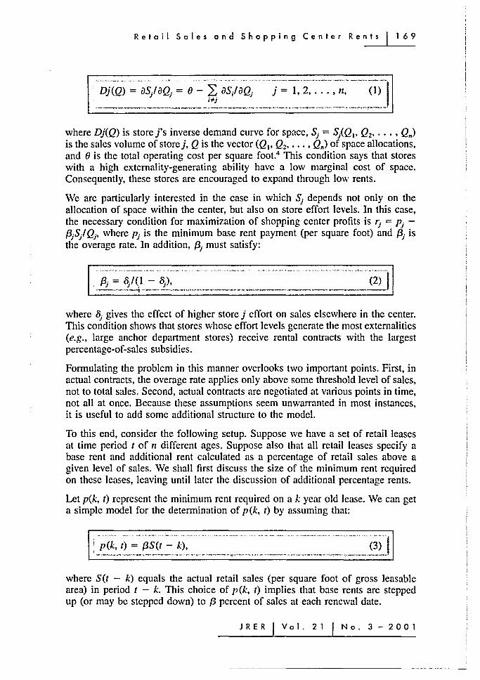
where Dj(Q) is store j's inverse demand curve for space, Sj = SiQI' Q2' .•. , Qn) is the sales volume of storej, Q is the vector (QI' Q2' •.• , Qn) of space allocations, and 0 is the total operating cost per square foot.4 This condition says that stores with a high externality-generating ability have a low marginal cost of space. Consequently, these stores are encouraged to expand through low rents.

We are particularly interested in the case in which Sj depends not only on the allocation of space within the center, but also on store effort levels. In this case, the necessary condition for maximization of shopping center profits is rj = Pj -{3jS/ Qj' where Pj is the minimum base rent payment (per square foot) and {3j is the overage rate. In addition, {3j must satisfy:

where 5j gives the effect of higher store j effort on sales elsewhere in the center. This condition shows that stores whose effort levels generate the most externalities (e.g., large anchor department stores) receive rental contracts with the largest percentage-of-sales subsidies.

Formulating the problem in this manner overlooks two important points. First, in actual contracts, the overage rate applies only above some threshold level of sales, not to total sales. Second, actual contracts are negotiated at various points in time, not all at once. Because these assumptions seem unwarranted in most instances, it is useful to add some additional structure to the model.

To this end, consider the following setup. Suppose we have a set of retail leases at time period t of n different ages. Suppose also that all retail leases specify a base rent and additional rent calculated as a percentage of retail sales above a given level of sales. We shall first discuss the size of the minimum rent required on these leases, leaving until later the discussion of additional percentage rents.

Let p(k, t) represent the minimum rent required on a k year old lease. We can get a simple model for the determination of p(k, t) by assuming that:

where Set - k) equals the actual retail sales (per square foot of gross leasable area) in period t - k. This choice of p(k, t) implies that base rents are stepped up (or may be stepped down) to {3 percent of sales at each renewal date.

JRER Vol.21 No.3-2001

- - ------- ------------------

170 (hun, Eppli and Shilling

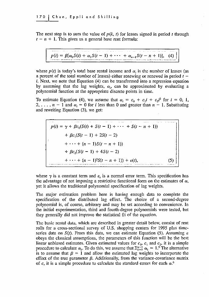
The next step is to sum the value of p(k, t) for leases signed in period I through I - 11 + 1. This gives us a general base rent formula:

where p(/) is today's total base rental income and a; is the number of leases (as a percent of the total number of leases) either renewing or renewed in period I -i. Next, we note that Equation (4) can be transformed into a regression equation by assuming that the lag weights, a;, can be approximated by evaluating a polynomial function at the appropriate discrete points in time.

To estimate Equation (4), we assume that a; = Co + cli + ci2 for i = 0, 1, 2, ... , II - 1 and a; = ° for i less than ° and greater than 11 - 1. Substituting and rewriting Equation (3), we get:

p(/) = 'Y + (3co(S(/) + S(t - 1) + ... + S(I - II + 1»

+ (3c l (S(t - 1) + 2S(t - 2)

+ ... + (ll - I)S(t - II + 1» + (3ciS(1 - 1) + 4S(t - 2)

+ ... + (11 - 1)2S(1 - 11 + 1» + e(/), (5) I

where 'Y is a constant term and e, is a normal error term. This specification has the advantage of not imposing a restrictive functional form on the estimates of a, yet it allows the traditional polynomial specification of lag weights.

The major estimation problem here is having enough data to complete the specification of the distributed lag effect. The choice of a second-degree polynomial is, of course, arbitrary and may be set according to convenience. In the initial experimentation, third and fourth-degree polynomials were tested, but they generally did not improve the statistical fit of the equation.

The basic rental data, which are described in greater detail below, consist of rent rolls for a cross-sectional survey of U.S. shopping centers for 1995 plus timeseries data on Set). From this data, we can estimate Equation (5). Assuming e obeys the classical assumptions, the parameters of this function will be the best linear unbiased estimates. Given estimated values for Co' C I and c2, it is a simple procedure to calculate ak • To do this, we assume that Lk:(~ ak = 1.5 The alternative is to assume that {3 = 1 and allow the estimated lag weights to incorporate the effect of the true parameter {3. Additionally, from the variance-covariance matrix of c, it is a simple procedure to calculate the standard errors for each a.6


In estimating Equation (5), a number of values of n arc tried, the first corresponding to 11 = 6, the longest lag we could obtain for retail sales. In order to assess the sensitivity of our results to this assumption, we also estimated Equation (5) assuming lags of four and five years (most specialty store tenants in a regional shopping center sign leases for five to ten years).

Turning now to the calculation of total rent, we let r(k, t) denote the total rent for leases originated in period t - k. The expected level of r(k, t) is defined by the following relationship:

r(k t) = {P(k, t) + (3(S(t) - S*(k, t» for S(t~ > S*(k, t) (6) , P (k, t) otherwise.

where S*(k, t) is the actual sales breakpoint specified in the lease. Now, summing over k, we have:

·;(;)"~'·~~;i·o·:·-t)·~··~':;(·i:~)'~-~-.. ~ ~n'~I~(;I' ~-1, t), _ ... _"'--(7)-'J -.-,~ .".-,. .......... - .... ~,.. .. ~ ,., ......... , .... ,,, .... ,'!'" ,~ ... -. 1- ......... - - '.-•••• -- ~" .. ,--, - ", ~'~-"'"--~""""" -," "--. .. -.- .... ,-~ .. -----.~-__ ,_ ..........

which can be used to make forecasts of total retail rents, both forward and backward in time beginning at time t, and to test for the responsiveness of rents to changes in retail sales.

Finally, we point out that the model in Equation (7) can lead to situations where the actual rate of change of r(t) may be opposite of that of S(t). First, we note that any arbitrary .1S(t) implies an associated Llp(t) of the form:

. _dp = ,-P (.:.....t _+_I~)_--,p--,(~t) dS Set + 1) - S(t)

[

(S(t) - Set - n + I)] g + Set)

= an-I (3, g

(8)

where g denotes the percentage rate of change in Set), i.e., g = .1S(t)/S(t). This result implies that dp/dS = a n- l {3 » 0 only when S(t) = S(t - 11 + I) and an-I

> 0, otherwise the value of dp/dS could be positive or negative, depending on the perturbation in Set) - S(t - n + 1) over the term of the lease. For example, in the case where g is negative, but where Set) - Set - 11 + 1) is positive, it is quite possible for dp/dS to be negative, implying p(t) should increase, rather than decrease, beyond t. By analogous reasoning, it also is quite possible for the reverse



to occur. That is, g could be positive, while Set) - Set - n + 1) could be negative, implying a decrease in pet) beyond t. This indeterminacy prevails whether actual contracts are negotiated all at once, i.e., an-I = 1, or at various points in time. It is only when we choose to work with 12 = 1 period leases instead of n = 5 or n = 10 period leases that dp/dS unambiguously becomes positive. In this special case, dp/dS takes on the value of {3, regardless of the past values of S(t), and with dp/p = (dp/dS)(dS/S)(S/p), dS/S = g, andp/S = (3, this implies dp/p = g, which is a very intuitive result.

Next, moving on to the relationship between the value of ret) and Set), it is important to distinguish between two separate cases: one where Set) < S*(k, t) for all k and one where Set) :::= S*(k, t) for all k. All other cases are simply some combination of these two. Where S(t) < S*(k, t) for all k, we have that:

dr r(t + 1) - r(t) - = ---"-----'------'-'-dS S(t + 1) - Set)

[

Set) - Set - 12 + 1)] g + S(t)

= an_I (3. g

(9)

This result is, of course, nothing but a replay of Equation (8). This is because, when Set) < S*(k, t) for all k, no tenant pays any overage, and, so, any effect of a higher Set) on ret) through higher overage rents is brushed aside, and the value of dr/dS in Equation (9) is automatically equal to the value of dp/dS in Equation (8).

A different outcome emerges, however, when Set) :2! S*(k, t) for all k. In this case, we have:

dr r(t + 1) - r(t) - = ~-~-----'''':;'' dS Set + 1) - Set)

g + Set) [

S(t) - S(t - n + 1)] = (1 - a n - I ){3 + all_I g {3. (10)

This result enables us, assuming S (t) = S (t - 12 + I), to write drl dS = (3. But this suggests that drl r, the rate of change in ret), should be equal to g, the rate of change in retail sales. This provides the intuition for Equation (10). For a value of Set) > Set - n + 1), on the other hand, the resulting value of dridS can be positive or negative, depending on the value of g. Likewise, for a value of

Reteil Seles end Shopping Center Rents 173

Set) < S(t - 11 + 1), the resulting value of dr/dS can also be positive or negative. Again, such results are critically dependent on the value of g.

As the data will show, another important parameter in this regard is the breakpoint! sales ratio, defined as S *(k, 1)/ S (I). Theoretically, the higher this ratio, the more gradual is the change in rents-the argument being that a change in retail sales will produce an immediate change in r(k, t), only if Set) rises above S*(k, t) (or if Set) starts out above S*(k, t»; otherwise, r(k, I) will only gradually change as leases are renewed and as p(k, t) is stepped up (or stepped down) to Set).

In the following sections, we turn to several numerical simulation analyses of the theoretical model. These simulations highlight interesting and nontrivial interactions of theoretical parameters, and also the difficulty involved in attempts to develop robust aggregate implications from such a framework. But before proceeding to the simulation analyses, we shall try to give an empirical account of the theoretical model and parameter values.

Estimation and Empirical Results

Data Description

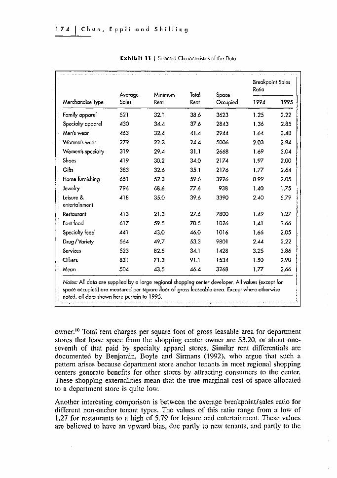
The basic data assembled for this study, mean values of pet), ret), Set) and S*(k, 1)IS(t) for tenants in U.S. regional shopping centers for 1995, are shown in Exhibit 11. The exhibit also contains average store size (in gross leasable square feet) and average lease term for various principal tenant types. The exact definition of each variable, the source of the data, their nature, and their derivation are all stated in considerable detail in the notes to the exhibit.7 Here the values are arranged according to major groups: department stores, clothing and accessories, shoes, home furnishings, home appliances/music, building materials/hardware, hobby/special interest, gifts/specialty, jewelry, drugs, personal services, food and food services.s

The data presented in Exhibit 11 show that jewelry stores, home furnishings, fast food restaurants and other services (including optical stores, pet shops, flower shops, stationers and news stands) are among the highest sales volume tenants (per square foot) in a regional shopping center. The mean sales volume, for example, for home furnishings and jewelry is between $650 and $800 per square foot of gross leasable area. The mean sales volume of all non-anchor tenants is $265 per square foot. Low sales volume tenants (excluding department stores) include women's wear, women's specialty and gifts.9

Because jewelry stores, fast food restaurants and other services are among the highest sales volume tenants in a regional shopping center, it comes as no surprise to find that they also are among the highest total rent tenants in a regional shopping center. The lowest total rent tenants (in rents per square foot) in a regional shopping center arc department stores that lease space from the shopping center

JRER Vol.21 No.3 - 2001


ExhIbit 11 I Selected Characteristics of the Data

Breakpoint Sales Ratio

Average Minimum Total Space Merchandise Type Sales Rent Rent Occupied 1994 1995

Family apparel 521 32.1 38.6 3623 1.25 2.22

Specialty apparel 430 34.4 37.6 2843 1.36 2.85

Men's wear 463 32.4 41.4 2944 1.64 3.48

Women's wear 279 22.3 24.4 5006 2.03 2.84

Women's specialty 319 29.4 31.1 2668 1.69 3.04

Shoes 419 30.2 34.0 2174 1.97 2.00

Gifts 383 32.6 35.1 2176 1.77 2.64

Home furnishing 651 52.3 59.6 3926 0.99 2.05

Jewelry 796 68.6 77.6 938 1.40 1.75

Leisure & 418 35.0 39.6 3390 2.40 5.79 entertainment

Restaurant 413 21.3 27.6 7800 1.49 1.27

Fast food 617 59.5 70.5 1026 1.41 1.66

Specialty food 441 43.0 46.0 1016 1.66 2.05

Drug / Variety 564 49.7 53.3 9801 2.44 2.22

Services 523 82.5 34.1 1428 3.25 3.86

Others 831 71.3 91.1 1534 1.50 2.90

Mean 504 43.5 46.4 3268 1.77 2.66

Noles: All data are supplied by a large regional shopping center developer. All values (except for space occupied) are measured per square Aoor of gross leaseable area. Except where otherwise noted, all data shown here pertain to 1995.

,'-, ... ~ .~. ,,-- ~ .. -. . ,. ~ .. ' _ .... _. -". _. ~ ~- . -'" . ~- _.-

owner. to Total rent charges per square foot of gross leasable area for department stores that lease space from the shopping center owner are S3.20, or about oneseventh of that paid by specialty apparel stores. Similar rent differentials are documented by Benjamin, Boyle and Sirmans (1992), who argue that such a pattern arises because department store anchor tenants in most regional shopping centers generate benefits for other stores by attracting consumers to the center. These shopping externalities mean that the true marginal cost of space allocated to a department store is quite low.

Another interesting comparison is between the average breakpoint/sales ratio for different non-anchor tenant types. The values of this ratio range from a low of 1.27 for restaurants to a high of 5.79 for leisure and entertainment. These values are believed to have an upward bias, due partly to new tenants, and partly to the


use of partial year sales. For this reason, we also report the average breakpointl sales ratio on leases in their first full year of operation. The values of this ratio (again for non-anchor tenant types) range from a low of 0.99 for home furnishings to a high of 3.25 in services, with a mean value of 1.77 (see Column 5 of Exhibit 11). These results suggest that retail sales, on average, must grow by 7.50% to 12% per annum over the remaining term of the lease-and in some cases as much as 16% per annum-if the tenant is ever to pay percentage rents. In the 1995 environment of, say, 3% expected inflation, it seems clear that most tenants will never pay overage rents. While most stores in a regional shopping center may be offered percentage-of-sales contracts rather than fixed rental contracts (see Benjamin, Boyle and Sirmans, 1992; and Miceli and Sirmans, 1995), these are generally far, far "out of the money" options and might reasonably be viewed as fixed rent contracts. This evidence is also difficult to reconcile with the view that percentage rent payments are smallest for stores that generate the most externalities (see Brueckner, 1993).

We assume in the rest of this article that the units of observation are regional shopping centers. This means, of course, that the variability of the data is greatly reduced. Nevertheless, there are many reasons why rents per square foot and sales per square foot will vary among regional shopping centers. Among the most important are differences in age of the shopping center, and recent rates of population and income growth. We proceed by regressing these average rents on present and past values of aggregate retail sales in a manner consistent with the statistical model described.

Empirical Estimates

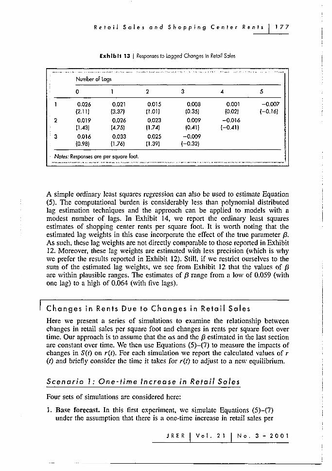
We estimated Equation (5) on our cross-section of shopping centers, with no endpoint priors. The results are presented in Exhibit 12. In all cases, the structure of the underlying model seems to fit the data reasonably well. The lag weights implied by the second-degree polynomial distributed lag model in Exhibit 12 are given in Exhibit 13, with standard errors reported in parentheses. It is apparent that lag length has a minor impact on the coefficient estimates. Nonetheless, several points should be made. First, Equations 1 and 2 in Exhibit 12 trace out a humped distributed lag. Both lag structures peak at a lag of one year, and then decline thereafter. Looking at the actual estimates, we find that the lag weights in Equation 1 turn negative after three years, while those in Equation 2 turn negative after two years. Second, the coefficients in Equation 3 result in a monotonically declining lag structure. The lag weights (on the assumption that the as sum to one) range from 0.42 in period t to 0.01 in period t - 4. In period t - 5, the lag weight is -0.11. Third, for the sum of the unadjusted coefficients (i.e., for the expression f3 ~k:J ak)' the respective values for Equations 1-3 are 0.061, 0.064 and 0.062. These are valid for a regional shopping center setting. They imply a percentage rental rate ranging from 6.05% to 6.40% of retail sales, which is entirely plausible.

JRER Vol.21 No.3 - 2001

Exhibit 12 I Estimates of Retail Rents

Coefficient Estimates Summary Statistics

Constant Co c. C2 C3 R2 Adj. R2 F-Value MSE

2.18 0.026 -0.005 -0.000 68.1 66.1 34.83 3.54 (1.42) (2.09) (-0.32) (-0.10)

2 1.97 0.019 0.013 -0.005 69.0 67.1 36.42 3.49 (1.29) (1.43) (0.61) (-1.05)

3 2.20 0.016 0.030 -0.013 68.5 66.5 35.47 3.52 (1.41) (0.97) (0.62) (-0.46)

4 1.94 0.011 0.081 -0.050 0.007 69.8 67.3 27.80 3.48 (1.28) (0.71) (1.50) (-1.67) (1.67)

5 2.09 0.014 0.050 -0.031 0.004 69.2 66.5 26.91 3.52 (1.34) (0.82) (0.57) (-0.52) (0.44)

6 2.19 0.016 0.029 -0.012 -0.000 68.5 65.8 26.06 3.55 (1.39) (0.90) (0.12) (-0.05) (-0.D1)

Noles: The dependent variable is minimum rents per square Foot. Estimates are per square foot. The t-Statistics are in parentheses. N = 52. ___ '~~R~~~

# of lags:

6

5

4

6

5

4

~ c: :I

m "U

"U

o :I

a.. c.n :r

:I

co


Exh Ib It 13 I Responses to logged Changes in Refail Sales

2

3

Number of Logs

o

0.026 0.021 (2.11) (3.37)

0.019 (1.43)

0.016 (0.98)

0.026 (.4.75)

0.033 (1.76)

Noles: Responses arc per square fool.

2

0.015 (1.01)

0.023 (1.74)

0.025 (1.39)

3 4

0.008 0.001 (0.35) (0.02)

0.009 -0.016 (0.41) (-0.41)

-0.009 (-0.32)

5

-0.007 (-0.16)

A simple ordinary least squares regression can also be used to estimate Equation (5). The computational burden is considerably less than polynomial distributed lag estimation techniques and the approach can be applied to models with a modest number of lags. In Exhibit 14, we report the ordinary least squares estimates of shopping center rents per square foot. It is worth noting that the estimated lag weights in this case incorporate the effect of the true parameter {3. As such, these lag weights are not directly comparable to those reponed in Exhibit 12. Moreover, these lag weights are estimated with less precision (which is why we prefer the results reported in Exhibit 12). Still, if we restrict ourselves to the sum of the estimated lag weights, we see from Exhibit 12 that the values of {3 are within plausible ranges. The estimates of {3 range from a low of 0.059 (with one lag) to a high of 0.064 (with five lags).

Changes in Rents Due to Changes in Retail Sales

Here we present a series of simulations to examine the relationship between changes in retail sales per square foot and changes in rents per square foot over time. Our approach is to assume that the as and the {3 estimated in the last section are constant over time. We then use Equations (5)-(7) to measure the impacts of changes in Set) on ret). For each simulation we report the calculated values of r (t) and briefly consider the time it takes for r(t) to adjust to a new equilibrium.

Scenario 1: One-time Increase in Retail Sales

Four sets of simulations arc considered here:

1. Base forecast. In this first experiment, we simulate Equations (5)-(7) under the assumption that there is a one-time increase in retail sales per

JRER Vol.21 No.3 - 2001

Exhibit 14 I OlS Estimates of Retail Rents Per Square Foot

Coemcient Estimates Summary Statistics

Constant Co c. C2 C3 C4 Cs f?2 Adj. f?2

3.64 0.06 63.2 62.5 (2.46) (9.36)

; 2 i

2.12 0.02 0.05 68.3 67.1 (1.42) (1.01) (2.84)

3 2.05 0.02 0.03 0.01 68.4 66.4 (1.35) (1.06) (0.61) (0.32)

;4 2.20 0.02 0.03 0.02 -0.01 68.5 65.8 , (1.39) (0.90) (0.62) (0.45) (-0.37)

5 2.09 0.01 0.04 0.02 0.00 -0.01 69.2 65.9 (1.32) (0.78) (0.74) (0.41) -0.16 (-1.03)

; 6 1.85 0.01 0.04 0.03 -0.01 -0.03 0.02 69.9 65.9 (1.16) (0.73) (0.73) (0.54) (-0.32) (-1.45) (1.04)

Notes: The dependent variable is minimun rents per square foot. The t-Statistics are in parenthesis. N = 53.

F-Value MSE

87.55 3.73

53.90 3.49

35.32 3.52

26.06 3.55

21.08 3.55

17.78 3.55

Sum of aj

0.059

0.064

0.064

0.064

0.061

0.064

~ C

::J

m "U "U

o ::J

0...

UI :r

::J

co


square foot of 10%. In addition, this simulation has S*(k, 1)/S(t) = 1.75, n = 6 and as == 0. 11 The simulation also uses historical values for past S(t - k).

2. Natural breakpoint experiment. In this experiment, the value of S*(k, t)/S(t) is reduced from 1.75 to 1.00 as a sensitivity test.

3. Shopping centers with growing sales. This experiment is identical to Simulation 1 except now, instead of using historical values for retail sales per square to forecast r(t), we assume that past sales per square foot were growing at 10% per year. This more rapid growth in retail sales per square foot should result in a more rapid growth of r(t).

4. Shopping centers with stagnant sales. In this last experiment, we assume that past retail sales per square foot are constant. The other parameters are the same as in experiment 3. The objective is to examine how r(t) adjusts in shopping centers with stagnant sales per square foot.

The results of the first two simulations are presented in Exhibit 15. The simulations suggest that rents are normally very slow to adjust to a new equilibrium. For instance, in our baseline simulation a one-time increase in retail sales per square foot of 10% causes rents to increase by slightly more than 8% over a six-year period. Of this increase, something like 20% of the adjustment occurs after three years, and then another 20% occurs in years four and five, with the remainder of the adjustment occurring in year six.

Under Simulation 2, we see that there is no adjustment lag effect. Here a onetime increase in retail sales per square foot of 10% leads to an immediate increase in rents per square foot of about 8%, as one would expect. When the breakpoint

ExhIbit 15 I Response to One-time Increase in Retail Sales of 10%

Rent adjustment with natural breakpoint 110 108 106

>( C!) 104 "0 ..: 102 .... c:

100 C!)

0:: 98

I ./

I ./ , ~

I ---- I Rent adjustment with saks breakpoint of 1.75

96 94

o 2 3 4 5 6 7 8 9 10

Adjustment Period (in years)

J R E R Vo I. 2 1 No.3-2001


!sales ratio is set equal to 1.00, the expression for ret) simplifies to ret) = f3S(t) for Set) > S*(k, t); and ret) = p(t) otherwise. Given this, a one-time increase in Set) of 10% should increase rents per square foot by f3 percent. Furthermore, this increase should occur all at once, rather than being spread out over several years. Note that in our case ret) goes up by slightly more than ~ percent owing to our simplifying assumption that as = O.

Our next two simulations address the question of path-dependency. From Equations (5)-(7), it is clear that the calculated values of ret) are enhanced by higher past values of Set). The procedure we propose to illustrate this is to simulate values of ret) using two different growth rates in past retail sales: one assuming a high growth rate and the other assuming a low (or zero) growth rate. These experiments suggest that, when past sales are constant, a 10% increase in retail sales per square foot causes rents per square foot to increase by slightly more than 8%, but that, when the same 10% increase in sales follows an annual growth rate in past sales of 10%, the percentage change in ret) is approximately 18% (see Exhibit 16). The explanation is that p(k, t) rises markedly upon lease renewal in the latter experiment, but not in the former experiment.

Scenario 2: One-time Decrease in Retail Sales

We now consider the effect of a one-time decrease in retail sales of 10% on rents per square foot. We do this by simulating the same four scenarios as above but with a one-time decrease in retail sales of 10% instead of a one-time increase in sales of 10%.

In our baseline simulation (with S*(k, t)/S(t) = 1.75, and as = 0), a one-time decrease in retail sales per square foot of 10% causes average rents per square

125

120

~ 115 '0

.5 110 i: ~ 105

100

95

Exh I bit 16 I Effect of Post Growth Rates in Retail Sales on Rent Increase

Rent adjustment assuming past growth rate of 1 ()';l; per annum

_\ .. - - -- - -- ---- -.. .-..

.. "...,...., + .-.. :""------Rent adjustment assuming Izero growth rate in retail sales ..

o 2 3 4 5 6 7 8 9 10



foot to fall by less than 1 % after three years, and by less than 3% after years five (see Exhibit 17). The surprising result is that by year six, the full impact of the decline is less than 5.5%. This result suggests that, because the base shifts, percentage increases and decreases in rents are not symmetrical (compare the results in Exhibit 15 with those in Exhibit 17).

Our next exercise is to simulate the rent adjustment process when the breakpoint! sales ratio, S*(k, 1)IS(I), is set equal to 1.00. Other than starting out at a slightly higher rate, these results do not vary much from the previous result.

We also simulate the change in r(l) resulting from a one-time decrease in sales, with and without a fairly large run-up in S(I) just prior to the fall in S(I) (see Exhibit 18). In the former case, rents per square foot actually rise in years two to five, before falling in year six. In the latter case, rents fall throughout, before stabilizing in years six to ten. These results are generally sensible. The temporary increase in rents in the former case comes about as old leases with low minimum base rents renew. They then decline thereafter as newer leases rollover at lower minimum base rents. In the latter case, both old and newer leases rollover at lower minimum base rents. Consequently, r(t) decreases monotonically over time.

Scenario 3: Actual Change in Retail Sales

In this simulation, we start out with data on actual retail sales per square foot for the years 1963-1995 from UU's survey of regional shopping centers. Average rents per square foot are then projected for the years 1968-1995 to the same tenant mix and quality of space that characterizes the regional shopping centers in Simulation 1.

102

100

~ 98 "0

.5 96 C ~ 94

92

90

Exhibit 17 I Response to One-time Decrease in Retail Soles of 10%

.... Rent adjustment with natural breakpoint

~

'" ~- Rent adjustment with sales breakpoint ratio of 1.75

"-"

o 2 3 4 5 6 7 8 9 10

Adjustment Period (in years) _-""'_"F>;-"_""~"~" ______ "".''''''''''''''''' __ ''''''' ___ ~~' ___ ''' __ '---'''''''_~'''_'' _______ ..... -- .. ",.~_!.-....--__ ."

J R E R Vo I. 21 No.3-2001


Exhibit 18 I Effect of Past Grovvth Rate in Retail Sales on Rent Decrease

106 104 102

>(

Rent adjustment assuming past growth rate of 10% per annum

.. - - -, tI .. .. .. , <I) 100 "0 c

98 -C 96 <:.I

p:: 94 92

.. --....... - -.. - .. - .. .. -- - -~~ __ Rent adjustment assuming zero

-........... growth rate an retail sales growth

" 90 o 2 3 4 5 6 7 8 9 10


The results of this simulation (deflated by the CPI deflator) are given in Exhibit 19. It is possible to get a rough idea of the relation between rents per square foot and sales per square foot over this time period by calculating a Pearson correlation coefficient in the following way. Note that observationally retail sales per square foot show less of a decline (in constant dollars) during the 1980s and 1990s than during the 1960s 'and 1970s. Also, during the 1980s, retail sales per square foot increased slightly, only to turn downward again in the 1990s.12 We find a Pearson correlation coefficient between our estimate of current rents per square foot and

Ex h I b It 19 I Simulated Shopping Center Rents vs. Actual Sales Per Square Foot (1968 = 100)

120

100 Rent -

80 x Q)

60 'C

t Sates

of: 40

20

0 <Xl 0 C\J ;:! CD ,.... ,.... 0> 0> 0> 0>

Year


actual sales per square foot of 0.97 (with a p-value of 0.0001) during the period 1968-1980. In contrast, similar calculations for the period 1981-1995 show a Pearson correlation coefficient between our estimate of current rents per square foot and actllal sales per square foot of 0.18 (with a p-value of 0.52). Over the entire 1968-1995 period, it appears that the Pearson correlation coefficient between our estimate of current rents per square foot and actual sales per square foot is 0.86 (with a p-value of 0.0001).

These results are noteworthy in several respects. First, the results suggest much the same predictions about the effects of retail sales growth on shopping center rents as in our first two scenarios-faster retail sales growth is associated with roughly proportionate higher rental growth, while a decline in retail sales will cause a roughly proportionate decline in rents. Second, as regards short-run dynamics, a faster rate of growth in retail sales will, at least in some neighborhood of time t, cause ret) to increase. This is attributable to the fact that any increase in ret) is conditional on the sluggishness inherent in the underlying retail lease agreements, which in some sense is the core point of the article. Third, the results indicate that ret) will overshoot its new, lower, equilibrium value and converge downward to it, when S(t - 11 + 1) < S(t + 1) < Set). Similarly, ret) will undershoot its new, higher equilibrium vallie and converge upward to it, when Set - Il + 1) > Set + 1) > Set). As regards the time path of r(t), from Exhibit 17 it is seen that while movements in S (t) do not induce exactly equal movements in the value of ret), the two values remain inextricably linked when looked at over the entire time period. This occurs, in large part, because the vallie of r(t) is projected to the same tenant mix and quality of space, which is in stark contrast to Exhibit 1-10.

Conclusion

This article has accomplished the following. We began by developing an economic model of retail rents. This model, which follows Brueckner's (1994) treatment of the optimal allocation of space in a regional shopping center, was then estimated using cross-sectional data on average rents per square foot combined with some corresponding time-series data on sales per square foot.

Interestingly, the evidence suggests that average rents per square foot in a regional shopping center generally do not respond immediately to a change in the incomegenerating capacity of the shopping center, but rather the response is "smoothed" out over time. Perhaps the most obvious reason for this rent smoothing is that most retail lease agreements in regional shopping centers are de facto, if not de jure, fixed lease arrangements. Part of this smoothing behavior also occurs because not all retail leases agreements are negotiated all at once. Consequently, during periods in which sales per square foot in a regional shopping center are rising (falling), average rents per square foot for most retail leases that are already in place will tend to remain relatively fixed. However, it is noted that some



adjustment in rents does occur as leases rollover (at which time minimum base rents are adjusted to some fixed percentage of retail sales).

We then used our cross-sectional estimates to make inferences about how rents per square foot would change from one equilibrium at a point in time to another equilibrium at a later point in time. This use depends on the assumption that the cross-sectional observations themselves represent equilibria, and that the model itself can be applied through time (i.e., that none of the parameters changes dramatically through time). The evidence suggests that average rents per square foot are not nearly as tied to retail sales as most observers would believe. The findings provide a useful perspective from which to view the theoretical models of retail rents reported above.

Endnotes

I A potential problem with Wheaton and Torto's (1995) analysis is that their data are not based on the same shopping centers over time, and, therefore, are not very comparable. Furthermore, in the 1960s and 1970s most regional shopping centers included one or more variety stores, one or more drug stores, and one or more supermarkets as leading tenants. During the 1980s and 1990s, most regional shopping centers repositioned themselves by shifting their emphasis from supermarkets, which have very high sales per square foot but low rent per square foot, to smaller specialty stores, like apparel stores, accessories, music and shoe stores, which have low sales per square foot but high rents per square foot. Then too, a noticeable movement has occurred away from the traditional arrangement in the 1960s and 1970s in which a department store leased space from the shopping center owner in the same general manner as other stores in the center. The current development trend is toward arrangements whereby the department store building is owned by the store itself, not by the shopping center owner, and one might expect this to have caused reported rents per square foot in regional shopping centers to rise over time.

2 This is in contrast to the main problem associated with longitudinal studies of shopping center rents, which is the difficulty of comparing rents and retail sales in a newly developed shopping center with those in a shopping center that has, over time, become more fully developed. The quality of the shopping center being different in the two cases is a source of error that can easily lead to the notion that rents have risen somewhat paradoxically over time, while what has, in fact, happened is that the risk of locating at that center has gone down markedly between the two dates, thereby causing shopping center rents to rise.

3 See also Eppli and Shilling (1995). They investigate the optimal time to develop a large regional shopping center.

4 Note that 0 is constant cross-sectionally, presupposing a single tenant improvement allowance. The theory also presupposes that all tenant improvements are paid for by the shopping center owner.

S As written, it is impossible to estimate Uk and {3 directly unless it can be assumed that LZ,:J Uk = 1.

6 The calculated standard errors are a function of the variance-covariance matrix of the


cs, appropriately weighted by the estimated values of Co' CI and c2• We can write the expression for var (a) as var (a) = var (co + cli + ci2

) = var (co) + P var (cl) + i4 var (c2) + 2i COl' (co. c l ) + 2P cov (co, c2) + 2P COl' (C., c2) for i = 0, 1, 2, ...• n - 1.

7 The data are proprietary, obtained from a single large shopping center developer/owner. Because the developer has asked to remain anonymous, many details cannot be made explicit. Information was collected not at the shopping center level, but specifically at t the tenant level.

g The data cover 178 stores and 8,538 specialty store tenants. Among the largest anchor tenants in the sample are JC Penney, Inc., Sears, Roebuck & Co., Dillard Department Stores, Federated. The May Department Stores, Montgomery Ward & Co., Inc., Dayton Hudson Corporation and Nordstrom, Inc. Among the specialty store tenants included are The Limited, F. W. Woolworth, Intimate Brands, The Gap, The Musicland Group, Edison Brothers Stores, Inc., County Seat and Borders.

9 Pashigian and Gould (1995) use reported sales per square foot from ULI's survey of shopping centers and find similar sales differentials across the various tenant types.

10 Six out of ten department stores in the sample own their own stores and the land underneath. Many department stores in the sample fall in both categories. That is, they lease space from some shopping centers, while owning their own stores in other shopping centers. For example, Montgomery Ward and Co., Inc. and JC Penney, Inc., own approximately 60% of their stores operated within the sample.

II Setting as equal to zero was done as a matter of convenience. While this formulation causes a slight overstatement in the calculated values of ret) (see text for more details), none of the qualitative results are changed when r(t) is calculated assuming as = 0 compared with those when ret) is calculated assuming as = -0.1138.

12 The decrease is especially noticeable during 1993-1995. One might have expected this decrease given the shifting priorities of the Baby Boomers away from apparel toward family-oriented home and electronic purchases.

References

Benjamin, J. D., G. W. Boyle and C. F. Sirmans, Price Discrimination in Shopping Center Leases, JOllmai of Urban Economics, 1992,32,299-317.

Brueckner, J. K., Inter-Store Externalities and Space Allocation in Shopping Centers, JOllmai of Real Estate Finance and Economics, 1993, 7, 5-16.

Chun, G., The Theory of Percentage Lease Contracts: The Case of Shopping Centers, University of Wisconsin, Unpublished Ph.D. dissertation, 1996.

Eppli. M. J. and J. D. Shilling. Large-Scale Shopping Center Development Opportunities, Land Economics, 1995, 71:1, 35-41.

J R E R Vo I. 2 1 No.3-2001


Miceli, T. J. and C. F. Sirmans, Contracting with Spatial Externalities and Agency Problems: The Case of Retail Leases, Regional Science and Urban Economics, 1995,25, 355-72.

Wheaton, W. C. and R. G. Torto, Retail Sales and Retail Real Estate, Real Estate Finance, 1995, 12,22-31.

Gregory H. Chun, University of Wisconsin, Madison. WI 53706 or [email protected]. edll.

Mark J. Eppli. George Washington University, Washington. DC 20052 or meppli@ gWll.edu.

James D. Shilling. University of Wisconsin. Madison. WI 53706 or js/Zilling@bus. wise.edll.

A Simulation Analysis of the Relationship between Retail Sales and Shopping Center Rents

Documents