A simple statistical-dynamical downscaling scheme based on weather types and conditional resampling

A simple statistical-dynamical downscaling scheme

based on weather types and conditional resampling

J. Boe,1 L. Terray,1 F. Habets,2 and E. Martin2

Received 15 November 2005; revised 12 June 2006; accepted 14 August 2006; published 15 December 2006.

[1] A multivariate statistical downscaling methodology is implemented to generatelocal precipitation and temperature series at different sites based on the results from avariable resolution general circulation model. It starts from regional climate properties toestablish discriminating weather types for the chosen local variable, precipitation in thiscase. Intratype variations of the relevant forcing parameters are then taken into accountby multivariate regression using the distances of a given day to the different weather typesas predictors. The final step consists of conditional resampling. The methodology isevaluated in the Seine basin in France. Using reanalysis fields as predictors, satisfyingresults are obtained at daily timescale and concerning low-frequency variations, both fortemperature and precipitation. The use of model results as predictors gives a realisticrepresentation of regional climate properties. Nevertheless, as the validation of a statisticaldownscaling algorithm for present day climate conditions does not necessarily imply thevalidity of its climate change projections, the plausibility of the downscaled climateprojections is assessed by verifying the consistency between spatially averageddownscaled results and direct model outputs for two climate change scenarios. Despitesome discrepancies for precipitation with the more extreme scenario, the consistency isgood for both local variables. This result reinforces the confidence in the use of thedownscaling scheme in altered climates. Finally, it is shown that the intertype variations ofthe atmospheric circulation represent only a fraction of the climate change signal for thelocal variables. Thus a downscaling methodology based on weather typing shouldincorporate information concerning intratype modifications.

Citation: Boe, J., L. Terray, F. Habets, and E. Martin (2006), A simple statistical-dynamical downscaling scheme based on weather

types and conditional resampling, J. Geophys. Res., 111, D23106, doi:10.1029/2005JD006889.

1. Introduction

[2] Water plays a central role in the behavior of the Earthsystem, and human activities are very dependent on waterresources. The question of water cycle modifications underclimate change conditions appears crucial, both to under-stand anthropogenic influence on climate and assess itsimpacts. Global modifications of precipitation are expectedto be important in terms of mean but also in terms ofstatistical distribution [Allen and Ingram, 2002; Trenberth etal., 2003]. To quantify the impacts of hydrological cyclemodifications at watershed scale, a solution would consist inusing an hydrometeorological model forced by the results ofa Coupled Atmospheric-Oceanic General Circulation Model(AOGCM). A major difficulty however exists following thisapproach: hydrometeorological models need most of thetime very high resolution forcings that AOGCM are unable

to provide. At present, a typical resolution for an AOGCMis 300 km, whereas hydrometeorological models often needdata with a resolution lower than 10 km. As a preliminarystep, methodologies must be consequently used to derivethe high-resolution forcings from the AOGCMs coarseresolution results: this is the downscaling issue.[3] Several studies interested by the modification of

different hydrological variables on French watersheds useda scale factor adjustment to obtain the high-resolutionforcings required for the hydrometeorological models[Etchevers et al., 2002]. Coarse-scale climate change projec-tions were applied to a high-resolution observed climatebaseline using the monthly anomalies between present andfuture climate simulation to modify current climate meteoro-logical parameters. This methodology eliminates the meanbiases due to the climate simulation upon the hydrometeoro-logical forcings but the modifications that occur at thesubmonthly level (concerning dry and wet spells or dailyextreme events for example) are not captured. To go further,other methodologies to bridge the scale gap betweenAOGCM and hydrometeorological models must be used.[4] Two main families of downscaling techniques can be

distinguished [Mearns et al., 1999]. A first approach, ordynamical downscaling, is a model-based methodology

JOURNAL OF GEOPHYSICAL RESEARCH, VOL. 111, D23106, doi:10.1029/2005JD006889, 2006ClickHere

for

FullArticle

1Climate Modelling and Global Change Team, Centre Europeen deRecherche et de Formation Avancee en Calcul Scientifique, Centre Nationalde la Recherche Scientifique, Toulouse, France.

2Centre National de Recherches Meteorologiques, Meteo-France,Toulouse, France.

Copyright 2006 by the American Geophysical Union.0148-0227/06/2005JD006889$09.00

D23106 1 of 20

leading to sub-AOGCM grid-scale features by most of thetime nesting a finer-scale Limited Area Model (LAM)within a GCM [Giorgi et al., 1990]. The current generationof LAMs have a typical resolution of about 50 km. Thesecond approach, statistical downscaling (SD), is based onthe idea that regional climate is conditioned by two factors:the large-scale circulation (LSC) that is well resolved by themodels, and small-scale features (e.g., land use, topography,land-sea distribution) that are not adequately described inGCMs [von Storch, 1999]. Thus an empirical relationshiplinking large-scale information (‘‘predictors’’) and local orregional variables (‘‘predictands’’) is first established forcurrent climate. Then, applying this empirical relationship,the local variables for future climate are derived from theLSC simulated by an AOGCM. This approach is based onthe strong hypothesis that the empirical relationship estab-lished for present climate is still valid under altered climateconditions [Wilby et al., 2004]. This ‘‘stationarity assump-tion’’ is the major theoretical weakness of SD as it is notverifiable (note that this limitation also exists for dynamicalmodel concerning the physical parameterizations).[5] The goal of this paper is to describe and validate a

new downscaling procedure intended to provide the high-resolution variables necessary to force the SAFRAN-ISBA-MODCOU (SIM) hydrometeorological model developed atMeteo-France [Habets et al., 1999] in order to investigatethe impacts of climate change on the Seine basin hydrologyin a future study. In this context, the downscaling method-ology must deal with multiple variables at an 8 km hori-zontal resolution. It is based on an hybrid dynamical/statistical approach. Terray et al. [2004] studied theresponse to climate change in terms of wintertime NorthAtlantic weather regimes and suggest that improved modelrepresentation of the atmospheric circulation at regionalscale is needed to achieve more reliable projectionsfor anthropogenic climate change on European climate.Moreover, the quality of the LSC simulated by the modelis a crucial point for statistical downscaling. For thesereasons, a variable resolution GCM of the atmosphere withhigher horizontal resolution over Europe is used to providethe predictors needed by the Statistical Downscaling Model(SDM).[6] This paper is divided into seven sections. Section 2 is

devoted to the description of the data and models used inthis study. Section 3 deals with the construction of thestatistical downscaling methodology and section 4 presentsits validation for current climate. In section 5 the perform-ances of the SDM using GCM outputs for current climateare assessed. In section 6 analyses based on climate changeprojection are described. The conclusions of our study arepresented in section 7.

2. Data Sets and Model

[7] The need for a downscaling procedure comes fromthe objective to study the impacts of climate change on thehydrological cycle of the Seine basin using the SIMhydrometeorological coupled system. In this system,SAFRAN [Durand et al., 1993] analyses the low-leveland surface atmospheric variables needed by the surfacescheme ISBA [Noilhan and Planton, 1989] such as precip-itation, incoming longwave and shortwave radiation fluxes,

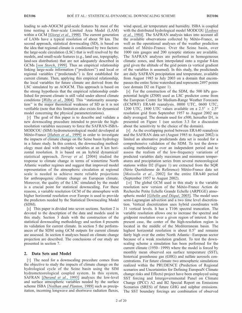
wind speed, air temperature and humidity. ISBA is coupledwith the distributed hydrological model MODCOU [Ledouxet al., 1984]. The SAFRAN analysis takes into account allthe available observations collected by Meteo-France, aswell as the operational analyses of the weather predictionmodel of Meteo-France. Over the Seine basin, over1000 rain gauges and 200 synoptic stations are available.The SAFRAN analyses are performed in homogeneousclimatic zones, and then interpolated onto a regular 8-kmgrid given the altitude of the grid points (a vertical gradientof the variables is assumed). In this study, the predictandsare daily SAFRAN precipitation and temperature, availablefrom August 1985 to July 2003 on a domain that encom-passes the entire Seine watershed and represents 2497 points(see domain D2 on Figure 1).[8] For the construction of the SDM, the 500 hPa geo-

potential height (Z500) used as LSC predictor come fromthe European Centre for Medium-Range Weather Forecasts(ECMWF) ERA40 reanalysis. 0000 UTC, 0600 UTC,1200 UTC, 1800 UTC values available on a 2.5� � 2.5�resolution grid from September 1957 to August 2002 aredaily averaged. The domain used for z500, hereafter D1, ispresented on Figure 1 (see section 3.3 for a discussionabout the sensitivity to the choice of the domain).[9] As the overlapping period between ERA40 reanalysis

and the SAFRAN data set (August 1985 to August 2002) islimited an alternative predictands data set is needed for acomprehensive validation of the SDM. To test the down-scaling methodology over an independent period and toassess the realism of the low-frequency variations ofpredicted variables daily maximum and minimum temper-atures and precipitation series from several meteorologicalstations within D2 (Figure 1) are extracted from the SQR(Serie Quotidienne de Reference) Meteo-France data set[Moisselin et al., 2002] for the entire ERA40 period(September 1957 to August 2002).[10] The global GCM used in this study is the variable

resolution new version of the Meteo-France Action deRecherche Petite Echelle Grande Echelle (ARPEGE) atmo-spheric model [Gibelin and Deque, 2003]. The model usessemi-Lagrangian advection and a two time level discretiza-tion. Vertical discretization uses hybrid coordinates with31 vertical levels. It has a T106 spectral truncation. Thevariable resolution allows one to increase the spectral andgridpoint resolution over a given region of interest. In thepresent case, the center of the high-resolution region islocated in the middle of the Mediterranean basin. Thehighest horizontal resolution is about 0.5� and remainsfairly high over the entire North Atlantic–European sectorbecause of a weak resolution gradient. To test the down-scaling scheme a simulation has been performed for thecurrent climate (1950–1999) where the model is forced bymonthly mean observed sea surface temperature (SST),historical greenhouse gas (GHG) and sulfate aerosols con-centrations. For future climate two atmospheric simulationsrealized within the PRUDENCE (Prediction of Regionalscenarios and Uncertainties for Defining EuropeaN Climatechange risks and Effects) project have been employed usingSST forcing and Intergovernmental Panel on ClimateChange (IPCC) A2 and B2 Special Report on EmissionsScenarios (SRES) of future GHG and sulphur emissions.The SST boundary forcings are combination of observed

D23106 BOE ET AL.: STATISTICAL-DYNAMICAL DOWNSCALING SCHEME

2 of 20

D23106

SSTs and mean SSTs changes derived from transient sim-ulations with the ARPEGE-Ocean Parallelise (OPA [Royeret al., 2002]) AOGCM for the B2 simulation and the ThirdHadley Center Coupled Ocean-Atmosphere General Circu-lation Model (HAD CM3 [Jones et al., 2003]) for the A2simulation. As the present day simulation described aboveis based on a slightly different version of the ARPEGEmodel, a control simulation with the same version as thefuture climate simulations is also used. It is forced bymonthly mean observed SST and historical GHG concen-trations for the period 1960–2000.

3. Downscaling Methodology

3.1. Concepts

[11] The most intuitive statistical downscaling approachis probably the analog method. This SDM is based on theidea that the same causes (here the LSC as predictor)produce the same effects (for the predictands, i.e., theregional climate). To obtain the local variables for aparticular day, the one with the most similar LSC patternis searched on the past observations given a measure ofdistance. Lorenz introduced the analog approach in the fieldof weather forecasting in 1969 but its use for downscalingpurposes is more recent [Zorita et al., 1995; Martin et al.,1997; Timbal, 2004]. This method which allows to deal withspatial and multivariate problems in a quite easy way givessatisfactory results. It often favorably compares with moresophisticated techniques [Zorita and von Storch, 1999] andcan thus be considered as a natural ‘‘benchmark’’ methodwhen developing a SDM. However, two difficulties arisewith the analog approach. First, the main weakness of all theempirical downscaling methods is that their basic assump-tion (i.e., that the statistical relationship established forpresent climate is still valid under altered climate) is notverifiable. In order to weaken this stationarity hypothesis it

is preferable to build a SDM that yields physically inter-pretable linkage between LSC predictors and regionalclimate [Wilby et al., 2004]. It is not the case for the analogmethod.[12] In addition, considering that the same causes in terms

of LSC give the same effects for the regional climate is animportant approximation. It is better to see the regionalclimate as a random process conditioned upon a drivingLSC [von Storch, 1999]. As the regional climate is notcompletely determined by the LSC, quasi-identical LSCpatterns can have large different effects in terms of regionalclimate [Roebber and Bosart, 1998]. Following this view,instead of searching only for the day with the nearest LSCpattern it could be preferable to search for an ensemble ofdays with similar LSC patterns and to consider the statisticaldistribution of the regional variables for these days.[13] The classical analog approach can be generalized in a

k-nearest neighbors analog method based on an ensemble ofanalog days [Gutierrez et al., 2004], but the first drawbackstill remains. Another possibility consists in using a smallnumber of weather types. Each day is classified in a weathertype and local variables are attributed depending on thistype. Two main issues are to address. The weather types,defined in terms of LSC similarity, should bring enoughinformation concerning the regional climate and a procedureto link local variables and weather types is necessary.Moreover, to be really more attractive than the analogmethod, the weather typing approach should be based ona small number of weather types (as the analog method canbe seen as a limit case of weather typing where each daydefines a weather type), in order to examine the physicalmechanisms that support the statistical model.[14] During the last decades, because of the development

of high-speed computers, objective automatic classificationalgorithms have been developed to complement oldersubjective schemes. In particular, the k-means algorithm

Figure 1. Location of the study area. (left) Domain used for the atmospheric predictors (D1) anddomain of SAFRAN predictands (D2). (right) Zoom on D2 and location of the meteorological stationsused as alternative predictands data set. Tmax and Tmin are daily maximum and minimum temperature,respectively, and Pre is precipitation.

D23106 BOE ET AL.: STATISTICAL-DYNAMICAL DOWNSCALING SCHEME

3 of 20

D23106

[Wilson et al., 1992] is now widely used in climate research.Given a prescribed number of clusters k and a measure ofsimilarity it searches to produce k clusters of greatestpossible distinction. The classifications in weather regimesby automatic classification algorithm can be useful when itcomes to explore the links between LSC and regionalclimate [Zhang et al., 1997; Corte-Real et al., 1999; Cassouet al., 2005]. Nevertheless, Plaut et al. [2001] showed thatthe classical North Atlantic weather regimes are not verydiscriminating for the French Alps precipitation. In order toobtain discriminating LSC patterns, they perform a prese-lection of the days characterized by heavy precipitationevents (defined in terms of fixed precipitation threshold)and then classify the corresponding LSC patterns with thek-means algorithm. This procedure leads to highly discrim-inating weather types for Alpine precipitation. This idea of abottom-up approach, which starts from local variable prop-erties to define discriminating weather types is retained inthis study. A data-driven method more adapted to thecontext and goal of this study is used to establish theprecipitation classes: the k-means algorithm is first usedto separate the precipitations within the domain D2 in a fewcharacteristic types. The LSC pattern of the days belongingto each precipitation types is then classified with thek-means algorithm. The priority is given to precipitationwhen building the weather types as it is the most importantvariable for hydrological application but it will be tested ifthe weather types are also discriminating for temperature.[15] The choice of predictor(s) is a major issue for statis-

tical downscaling. Predictor(s) must have strong predictiveskills for the predictands in present climate, but also besensitive to climate change signal [Wilby et al., 1998].Conversely, a predictor that does not seem to be importantfor present climate could become essential under perturbedclimate conditions. For instance, it is suspected that futurechanges in surface temperature will be dominated by changesin the radiative properties of the atmosphere, rather than bycirculation changes [Schubert, 1998]. Thus the use of a singledynamical predictor could be problematic when one isinterested in temperature. Another example concerns precip-itation: the changes in the water-holding capacity of theatmosphere (linked with temperature change through theClausius-Clapeyron equation) is supposed to play an impor-tant role on precipitation changes [Allen and Ingram, 2002].Coherently, some studies show that the inclusion of humidityas a predictor can have significant impacts on the results of aSDM [Charles et al., 1999]. In addition, the predictors shouldalso be realistically simulated by theGCMs and this conditionmight be a major constraint for the choice of predictors. Ingeneral, more confidence is given to the simulated large-scaledynamical variables. The use of thermodynamical variableslike surface temperature or humidity, for which the local andsurface effects can be important is more questionable. Thisissue will be addressed in the following. A downscalingprocedure which only uses a LSC predictor will be comparedto one that incorporates in addition temperature or humidityinformation from the model.

3.2. Application: Weather Typing Approach

3.2.1. Derivation of the Weather Types[16] The first step of the downscaling process consists in

establishing the weather types (step 1 on Figure 2). A

k-means classification of SAFRAN precipitations is realizedon D2 for the learning period (August 1985 to August 2002).Three seasons are considered. Traditional summer (June toAugust, JJA) and winter (December to February, DJF)seasons are kept and spring and autumn days are gatheredto constitute the third season for the classification. Onlyconfigurations with two or three clusters per season aretested as the spatial variations of precipitations are quitehomogeneous on the domain.[17] The days belonging to each precipitation cluster are

then classified depending upon their LSC. Daily maps of500 hPa geopotential height are classified within eachprecipitation cluster over the domain D1 with the k-meansalgorithm in the subspace of the first ten Principal Compo-nents (PC), accounting for more than 95% of the explainedvariance. This number of PCs is considered sufficient tocapture the main features of Z500 variability. Here, the PCshave not been scaled with their eigen values to have unitlength. Nevertheless, note that when the PC are scaled orwhen the number of PCs retained is modified, the results ofthe classification are essentially the same. The major draw-back of the k-means algorithm is that the number k ofclusters must be chosen a priori. Different approaches areused to determine the optimal value of k, but no consensusexists. Here, two tests are employed: the test based on aclassifiabilty index described by Michelangeli et al. [1995],and the test based on a inter/intra cluster variance ratio usedby Straus and Molteni [2004]. Following those twoapproaches, k varying between two and five are tested foreach precipitation cluster. Only solutions for which the twotests are coherent are kept. When there is no valid solution,a composite including all the days within the precipitationcluster is alternatively used. As several valid combinationsstill remain after the two tests, the most discriminatingcombination of weather types in terms of precipitation issearched. An inter/intra cluster variance ratio is computedfor precipitation for each valid combination of weathertypes and the configuration with the highest ratio is chosen.[18] The precipitation clusters obtained mainly differ by

their global intensity on D2. For the sake of simplicitythey will be thus hereafter designated given their observedcharacteristics (not shown) as ‘‘dry,’’ ‘‘wet’’ or ‘‘very wet.’’Table 1 shows the number of weather types obtained foreach season and associated with the three precipitationclusters.[19] The procedure described above based on precipita-

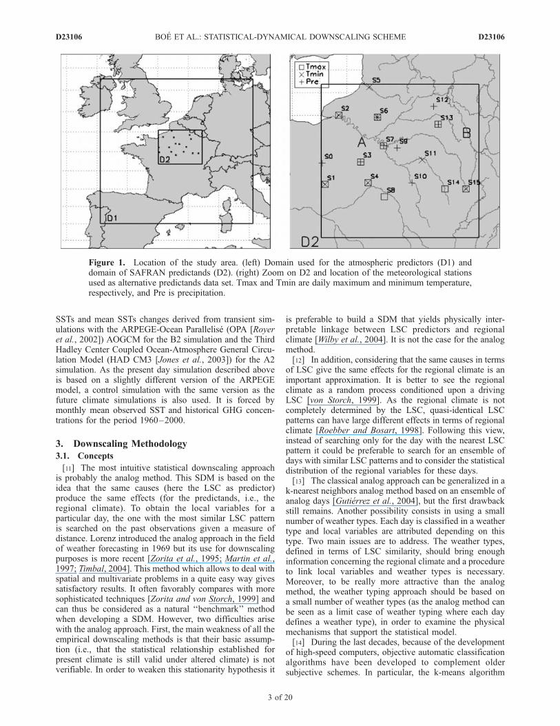
tion clustering is only a preliminary step to establish theLSC weather types. Once the weather types have beenobtained, each day is associated to a weather type depend-ing only on it LSC. The nearest weather types in terms ofEuclidian distance between the daily map of Z500 and theweather types is searched (step 2 on Figure 2). Figure 3shows the Z500 anomalies that correspond to each winterweather type and Table 2 presents spatially averaged char-acteristics of rainfall and temperature for each winterweather type. WT0, related to the ‘‘very’’ wet precipitationcluster, is characterized by a dipole pressure pattern with avery strong Z500 negative anomaly centered over theBritish isles, and a weaker positive anomaly over Algeria.The pronounced zonal flow over the Seine basin leads tovery warm and wet conditions on D2 (Table 2). For thisweather type, 98% (96%) of the days have greater rainfall

D23106 BOE ET AL.: STATISTICAL-DYNAMICAL DOWNSCALING SCHEME

4 of 20

D23106

(temperature) than the global winter median. WT1, obtainedfrom the ‘‘wet’’ precipitation cluster, is quite spatiallysimilar to WT0, although less intense. WT1 is also relatedto warm and wet anomalies over D2, but less intense thanwith WT0. The last three weather types are derived from the‘‘dry’’ rainfall cluster. WT2 features a strong anomaloushigh over the North Sea and corresponds to very drycondition on the Seine basin. WT3 is close to the meanstate both in terms of rainfall and LSC pattern (note that thisweather type occurs only 26% of the time). With a negativeZ500 anomaly centered on the study area, WT4 circulationis characterized by anomalous northeasterlies leading toadvection of cold air and snow type events. 64% of snowfallamounts occur within this weather type (which representsonly 0.10 mm/day as snowfall on the domain D2 is not verylarge).3.2.2. Downscaling Algorithms[20] Weather is a continuous process and discretizing it

into discrete states can rise issues in downscaling context asnoted by Mehrotra and Sharma [2005] who present analternative approach based on continuous weather states. Inparticular, intratype variations concerning the regional cli-mate may not be captured [Wilby et al., 2004]. Themethodology described above leads to weather types thatare really discriminating for precipitation on D2. They alsoprove their efficiency in discriminating temperature eventseven if they have not been explicitly constructed for thelatter. Nevertheless, when looking at the standard deviationof rainfall amounts and temperature for each weather type inTable 2 it is also seen that intracluster variability in terms of

regional climate is not negligible. Intracluster regionalclimate variability has two causes. A spread of LSC patternswithin a given weather type exists and the regional climateis not entirely determined by the LSC. Considering thesimilarity between the circulation of a particular day and theweather types is a way to deal with the LSC intraclustervariability. In particular, Plaut [2004] showed that strongrelationships exist between precipitation in the Alpes Mar-itimes (France) and the similarity to some particular circu-lation patterns. Here, the distances to the weather types areused to better capture intracluster variability. The distancedk(t) between the LSC of day t and the weather type k ismeasured by an Euclidean distance computed over the tenfirst principal components of Z500 (step 20 on Figure 2):

d2k tð Þ ¼X10i¼1

ai tð Þ � Aki

� �2 ð1Þ

where ai refers to Z500 PC scores and Aik to the coordinates

of the weather types k in the PC-space. PC have been scaledto have unit variances.

Figure 2. Flowchart presenting the main step of the downscaling algorithm ‘‘weather typing 1’’ for aseason. Pr is precipitation, Ta is temperature and Z500 is 500 hPa geopotential height. WT is weathertype. Ci

Pr is the ensemble of the days that belong to the precipitation cluster i. CiZ500 is the ensemble of

the days that belong to the weather type i. The bk are the regression coefficients and a the constant of theregression equations (index Ta for temperature and index Pr for precipitation).

Table 1. Number of Weather Types Retained for Each Season

Depending on the Precipitation Class

Precipitation Cluster Winter Summer Spring/Autumn

Very wet 1 1 1Wet 1 1 1Dry 3 4 4

D23106 BOE ET AL.: STATISTICAL-DYNAMICAL DOWNSCALING SCHEME

5 of 20

D23106

[21] The N daily series of distances corresponding to theN weather types of the season are used as predictors in amultiple linear regression. The predictand is the spatialmean of precipitation on D2, hPr(t)i (here and hereafterthe symbol h.i refers to the spatial mean on D2). Because ofthe skewed character of daily precipitation, the precipitationseries is transformed before solving the regression equation(note also that only the spatial average, less skewed, is usedhere). A square root transformation is applied. For the

learning period the following regression equation is thussolved:

hPr tð Þi1=2 ¼XNk¼1

bk :dk tð Þ½ þ aþ e tð Þ ð2Þ

where the bk are the regression coefficients, a a constantand e(t) the residuals. The high multiple linear correlation

Figure 3. Winter weather types: Z500 anomalies composite (gpm). WT0 corresponds to the very wetprecipitation cluster, WT1 to the wet precipitation cluster and WT2, WT3 and WT4 to the dryprecipitation cluster.

D23106 BOE ET AL.: STATISTICAL-DYNAMICAL DOWNSCALING SCHEME

6 of 20

D23106

coefficients obtained (between 0.64 and 0.71 according tothe season) indicates that a strong physical link actuallyexists between the distances to the weather types and theprecipitation on D2 at the daily level. During the down-scaling procedure, the regression equation is used tocompute a precipitation index that only depend upon LSC(Z500). As the temporal variance of the precipitation indexcomputed by linear regression is underestimated, its directvalues are not used in the algorithm. Instead, the values ofthe index are classified into ten equally populated categoriesand only these categories are considered. This procedure issimilar to the one described in Plaut [2004].[22] To take into account temperature, two different

approaches are tested. In the first one, a temperature indexis computed using a multiple linear regression with thedistances to the weather types as predictors as in theprecipitation case. A high multiple linear correlation coef-ficient is also obtained (between 0.66 and 0.77). Thismethod, named hereafter ‘‘weather typing 1,’’ only uses alarge-scale dynamical predictor (Z500). Note that thisscheme does not directly account for the radiative compo-nent associated with global temperature increase. Thisscheme is thus likely to be partly insensitive to climatechange signal, in particular for temperature. To overcomethis intrinsic drawback and to assess its potential associatedimprovement an alternative procedure is proposed. In thissecond procedure the temperature index based on LSCdescribed above is not used. Instead, the direct temperaturefrom the model for which the downscaling is needed (orfrom ERA40 in case of validation) is averaged on D2 andused as temperature index. This downscaling algorithm ishereafter named weather typing 2.[23] In the two approaches the final step of the down-

scaling algorithm is identical. It consists of conditionalresampling from the historical record (step 3 on Figure 2).[24] To recapitulate, once the weather types have been

derived, three steps are necessary to downscale GCM out-puts or reanalysis data for a particular day (step 2,20, and 3on Figure 2). First, the day is classified in the nearestweather type. Next, using the regression coefficients esti-mated for the learning period, the value of the precipitationindex for this day is computed. For temperature, withthe weather typing 1 method, the temperature index iscomputed in the same way as for precipitation. Withweather typing 2, the temperature from the GCM averagedon D2 is used as temperature index. Finally, a day from thelearningperiod that belongs to the sameweather type, andwithprecipitation and temperature indices belonging to the samedeciles is randomly chosen. If there is no overlapping day

between the three conditions in the learning period, thoseconcerningtheweathertypeandtheprecipitationindexremain,and the neighboring quantiles are searched for temperature.[25] In the following, the results obtained with the weather

typing approaches are compared with those obtained by theanalog method. A detailed description of the analog methodis presented in Zorita and von Storch [1999]. In our case, thedistance between the circulation of two days necessary inthe analog algorithm is computed in the space spanned bythe ten first principal components of the predictor. The LSCdomain (D1) and predictor (Z500 only) are the same as forweather typing 1 in order to allow the comparison of the twomethods.

3.3. Sensitivity to Different Parameters

[26] Several choices have been required during the con-struction of the SDMs. Mainly, the domain for the LSCpredictor, the LSC variable used as main predictor, and theseasonal stratification during the construction of the weathertypes. To evaluate the impacts of these choices, differentsensitivity tests have been performed. Different domains forLSC predictors have been tested: from a small domaincentered on France to the entire North Atlantic sector. Alarge domain sometimes gives an improved representationof spell properties, in particular for the analog method (asthe LSC on the North Atlantic sector for a particular dayprovides also information about the LSC for Europe for theforthcoming days). Nevertheless, the correlations betweenoriginal and downscaled series with predictors from ERA40reanalysis quickly decrease when the domain is enlarged, inparticular for precipitation. To account for a realistic simu-lation of the LSC by the GCM, the domain must also not betoo small. The domain D1 finally used here appeared as thebest compromise. Mean sea level pressure and 700 hPageopotential height have been tested instead of Z500. Theoverall performances of the SDMs used in this study arerather insensitive to the choice of the LSC predictor. For theweather classification three seasons have been chosen(winter (DJF), summer (JJA), and the rest of the months).It appeared important to keep only DJF months for winterand JJA months for summer. When these seasons areextended a deterioration of the downscaling results is seen.Conversely, separate spring and autumn days for the clas-sification does not improve the results. With the weathertyping methods, at the conditional resampling stage, tencategories are used for the temperature and precipitationindices. This is a conservative choice allowing for largeresampling sets for the majority of the days. More catego-ries can improve the results of the two downscaling schemes

Table 2. Area-Averaged (D2) Rainfall and Temperature Characteristics Depending Upon the Weather Type for Winter (1985–2002)a

WT0 WT1 WT2 WT3 WT4 All Days

Occurrence 9.1% 8.9% 40.5% 23.6% 17.7%Percentage of days with rainfall > global median 98% 88% 27% 55% 53% 50%Rainfall amounts, mm/day 7.50 (5.27) 4.63 (3.93) 0.79 (1.59) 2.06 (2.99) 2.02 (2.69) 2.27 (3.49)95th percentile of rainfall amounts, mm/day 19.47 12.62 4.36 7.82 7.13 9.26Percentage of days with temperature > global median 96% 81% 49% 43% 21% 50%Mean temperature, K 281.1 (2.23) 279.2 (2.98) 277.5 (3.71) 276.4 (3.71) 274.2 (4.04) 277.1 (4.06)95th percentile of temperature, K 284.6 282.8 283.5 281.8 279.6 283.3

aStandard deviation is shown in brackets.

D23106 BOE ET AL.: STATISTICAL-DYNAMICAL DOWNSCALING SCHEME

7 of 20

D23106

with the ERA40 predictors, but with the ARPEGE ones, thepicture is less clear.

4. Validation of the Downscaling Algorithms

4.1. SAFRAN Predictands

[27] The two weather typing methods are applied and theresults are compared with those obtained by the analogmethod. In this section, Z500 comes from the ERA40reanalysis and predictands are SAFRAN daily precipitationand temperature. Downscaling results are evaluated for theentire learning period (August 1985 to August 2002). Notethat when searching the analog of a specific day, the latterand its ten predecessors and successors are rejected fromthe possible resampling set in order to avoid artificial skill.The predictand time series are reconstructed day by dayand the relative performances of the three SDMs are as-sessed by first comparing different skill scores already usedin Timbal et al. [2003]. Linear correlations are computedbetween observed and reconstructed series (unless specifiedotherwise, here and hereafter all the correlation coefficientsgiven are significant at the 0.05 level, using the ‘‘random-phase’’ test accounting for autocorrelation described inEbisuzaki [1997]). Brier score (BS) is defined as:

BS ¼ 100� 1� MSE

MSEref

� �ð3Þ

where MSE is the Mean Square Error for downscaled seriesand MSEref the one for a reference scheme: here, a purelyrandom choice of analogs. BS varies between 100%(perfect forecast) and 0% (random choice of analogs). Forprecipitation, an additional score (Ind) quantifying the skillof the SDM in reproducing rain occurrence is defined as:

Ind ¼ 100� 1� m

wþ m� f

d þ f

� �ð4Þ

The letter w stands for a wet day both forecast and observed,d to a dry day both forecast and observed, m to a wet daymissed by the forecast and f to a dry day missed by theforecast (here and hereafter a dry day is defined as a daywith no rain). For a perfect forecast Ind equals 100%.Scores are computed for each grid point and then averagedover the entire domain.[28] For temperature, as expected since ERA40 tempera-

ture information is incorporated through the downscalingprocess, the skill scores are better for weather typing 2 thanothers (Table 3). Weather typing 1 and analogs give very

similar results. Concerning precipitation, the two weathertyping schemes perform better than the analog method.Brier scores and correlations are weaker than for tempera-ture (precipitation is well known to be a difficult variable todownscale), but skill exists. Note that at the monthly levelthe correlations between reconstructed and original precip-itation series is much higher (between 0.63 and 0.75 on D2with weather typing 1).[29] Correlation between downscaled and original series

can be a good indicator of the relative performances ofdifferent SDMs, but it might be misleading. To assess thehydrological impacts of climate change, it is important thatstatistical properties like first and second moments, persis-tence, extremes are well represented. However, in theempirical downscaling context, the objective to obtain thebest correlation and the objective to obtain the best repre-sentation of some statistical properties, like daily variance,are often conflicting. For example, regression-based meth-ods are known to give good time correlation but also to tendto strongly underestimate temporal variance [Zorita and vonStorch, 1999]. Here, with an analog based approach, a bettercorrelation could also be achieved. If instead of consideringonly a single analog, the means of local variables arecomputed for the five days with the most similar LSCpatterns, the correlation for precipitation practically doublesbut the daily variance becomes greatly underestimated.[30] Table 4 introduces several diagnostics of daily pre-

cipitation concerning first and second moments, extremes,persistence, used by Wilby et al. [1998]. These diagnosticsare computed for original and downscaled precipitations(Table 5). Each diagnostic is computed on each point of D2for the four seasons. Mean and RMSE are then computed onthese values (4 seasons by 2497 points values). Globally,the results from the different SDMs are close to theobservations. Mean, SD wet, 95% wet and pd are wellrepresented (but a purely random resampling of the learningperiod days would also be successful). Persistence proper-ties (pdd, pww and spell diagnostics) are also well reproducedby the weather typing methods. These latter properties arevery important for hydrological applications and moredifficult to achieve. The major differences between weathertyping and analog methods concern pdd, pww and Ld as theanalog method underestimates these properties.[31] Mean, standard deviation, 95th percentile were also

computed for downscaled and original temperature series.These properties are very well reproduced by all themethods (not shown).

Table 3. Skill Achieved by the Different Downscaling Models for

Daily Temperature and Precipitation (1985–2002)

Variable Analog Weather Typing 1 Weather Typing 2

PrecipitationCorrelation 0.17 0.30 0.31Brier score 18 29 30Ind 25 35 35

TemperatureCorrelation 0.85 0.85 0.93Brier score 85 86 93

Table 4. Standard Precipitation Diagnostics

Daily Precipitation Diagnostics

Mean mean wet-day amount, mmSD wet standard deviation of wet day amount, mm95% wet 95th percentile of wet day amount, mmpd unconditional probability of a dry daypdd probability of a dry day conditional

on the previous day being drypww probability of a wet day conditional

on the previous day being wet

Spell Diagnostics

Lw mean wet spell length in daysLd mean dry spell length in days

D23106 BOE ET AL.: STATISTICAL-DYNAMICAL DOWNSCALING SCHEME

8 of 20

D23106

4.2. Alternative Predictands Data Set

[32] When validating a SDM, it is particularly importantto test its ability to reproduce low-frequency variations ofpast climate, like trends or oscillations, as it can beconsidered as a sort of ‘‘natural’’ climate change [Zoritaand von Storch, 1999]. Several downscaling methods, inparticular stochastic weather generators and also somecirculation-based methods, often greatly underestimatelow-frequency variability [Wilby et al., 1998]. As the lengthof the SAFRAN data set is quite short, the validation of thelow-frequency variability of downscaled variables is prob-lematic. Moreover, the previous diagnostics were computedfor a period identical to the learning period, which canhamper the conclusions. To address these two problems,several meteorological station observations are now used asalternative predictands (section 2, Figure 1). Eight precip-itation, ten maximum temperature (Tmax) and seven min-imum temperature (Tmin) stations are available with nomissing values for the complete ERA40 reanalysis period(1957–2002) on D2. Five stations provide both Tmax andTmin, and hereafter temperature indicates the mean betweenTmax and Tmin for these stations. The three SDMs areapplied with these new predictands. The local variables arereconstructed for all the ERA40 period (1957–2002) withthe same learning period as previously (1985–2002).[33] RMSE and mean correlation between reconstructed

and original local variables series for the learning period,the independent period (September 1957 to August 1985)and the entire period are given in Table 6. The resultsobtained for the learning period and for the independentperiod are very similar. Here, using the same period for theconstruction and the validation of the SDMs does not leadto artificial skill.[34] The interannual variability of original and down-

scaled series is now explored. Table 7 shows the meancorrelations between seasonally averaged series of temper-

ature and precipitation. Concerning precipitation, the twoweather typing approaches clearly outperform the analogmethod for all the seasons. The best results are obtained forwinter and the worst for summer independently of theSDMs. The convective nature of precipitation in summerprobably explains the weaker link between LSC and pre-cipitation for this particular season.[35] As expected by construction, for temperature, weather

typing 2 is the best SDM in all seasons. For summer andwinter weather typing 1 gives also very good resultswhereas for spring and autumn correlations are weaker.The worst results are obtained with the analog methodwhatever the seasons.[36] To further pursue the study of low-frequency varia-

tions at different timescales, downscaled and original dailyseries of temperature and precipitation are filtered usingdifferent Hanning window width, and correlations betweenobserved and downscaled series are computed. Results areplotted on Figure 4.[37] In order to see if the use of humidity predictor from

ERA40 reanalysis allows to better capture time variabilityof precipitation, an additional weather typing method is alsoused. It corresponds to a modified version of weathertyping 2 where temperature as secondary predictor isreplaced by ERA40 1000 hPa humidity (this method isnamed weather typing 2bis). With this alternative secondarypredictor, at daily timescale, the results for the diagnosticsdescribed in section 4.1 are very similar with those obtainedwith temperature predictor (not shown). For temperature, upto 365 days, all the methods give high correlations. Oncethe annual cycle is filtered only weather typing 2 is able towell reproduce the temporal variations while the othermethods lead to an important decrease of correlation. Thedifference between weather typing 1 and weather typing 2results seems to indicate that a part of temperature low-frequency variability is not driven by LSC as the use oftemperature as secondary predictor seems to be required to

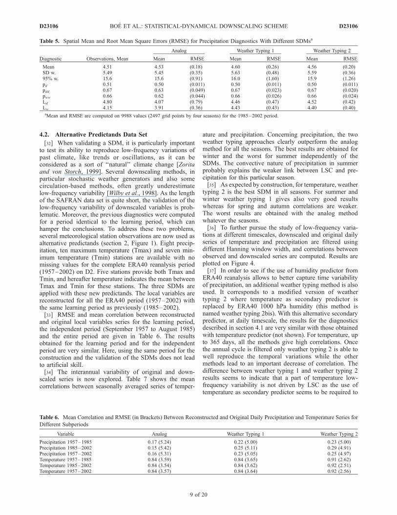
Table 5. Spatial Mean and Root Mean Square Errors (RMSE) for Precipitation Diagnostics With Different SDMsa

Diagnostic Observations, Mean

Analog Weather Typing 1 Weather Typing 2

Mean RMSE Mean RMSE Mean RMSE

Mean 4.51 4.53 (0.18) 4.60 (0.26) 4.56 (0.20)SD w. 5.49 5.45 (0.35) 5.63 (0.48) 5.59 (0.36)95% w. 15.6 15.6 (0.91) 16.0 (1.60) 15.9 (1.26)pd 0.51 0.50 (0.011) 0.50 (0.011) 0.50 (0.011)pdd 0.67 0.63 (0.049) 0.67 (0.023) 0.67 (0.020)pww 0.66 0.62 (0.044) 0.66 (0.026) 0.66 (0.024)Ld 4.80 4.07 (0.79) 4.46 (0.47) 4.52 (0.42)Lw 4.15 3.91 (0.36) 4.43 (0.43) 4.40 (0.40)aMean and RMSE are computed on 9988 values (2497 grid points by four seasons) for the 1985–2002 period.

Table 6. Mean Correlation and RMSE (in Brackets) Between Reconstructed and Original Daily Precipitation and Temperature Series for

Different Subperiods

Variable Analog Weather Typing 1 Weather Typing 2

Precipitation 1957–1985 0.17 (5.24) 0.22 (5.00) 0.23 (5.00)Precipitation 1985–2002 0.15 (5.42) 0.25 (5.11) 0.29 (4.91)Precipitation 1957–2002 0.16 (5.31) 0.23 (5.05) 0.25 (4.97)Temperature 1957–1985 0.84 (3.59) 0.84 (3.65) 0.91 (2.62)Temperature 1985–2002 0.84 (3.54) 0.84 (3.62) 0.92 (2.51)Temperature 1957–2002 0.84 (3.57) 0.84 (3.64) 0.92 (2.56)

D23106 BOE ET AL.: STATISTICAL-DYNAMICAL DOWNSCALING SCHEME

9 of 20

D23106

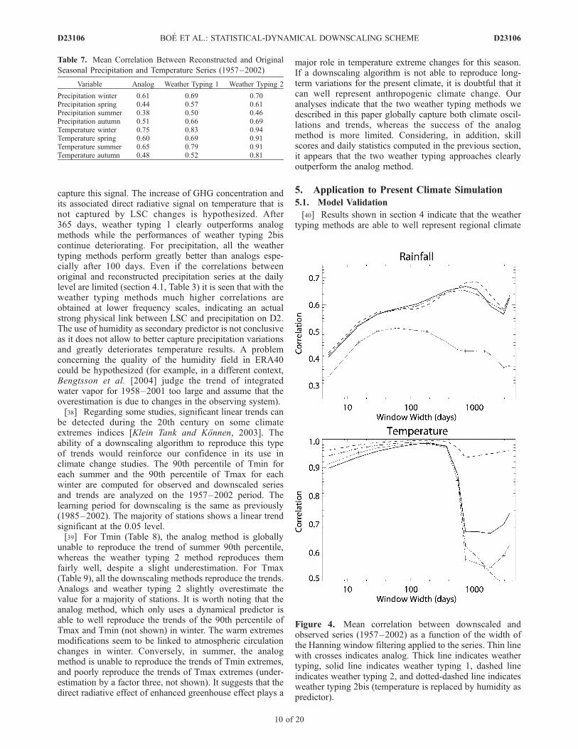
capture this signal. The increase of GHG concentration andits associated direct radiative signal on temperature that isnot captured by LSC changes is hypothesized. After365 days, weather typing 1 clearly outperforms analogmethods while the performances of weather typing 2biscontinue deteriorating. For precipitation, all the weathertyping methods perform greatly better than analogs espe-cially after 100 days. Even if the correlations betweenoriginal and reconstructed precipitation series at the dailylevel are limited (section 4.1, Table 3) it is seen that with theweather typing methods much higher correlations areobtained at lower frequency scales, indicating an actualstrong physical link between LSC and precipitation on D2.The use of humidity as secondary predictor is not conclusiveas it does not allow to better capture precipitation variationsand greatly deteriorates temperature results. A problemconcerning the quality of the humidity field in ERA40could be hypothesized (for example, in a different context,Bengtsson et al. [2004] judge the trend of integratedwater vapor for 1958–2001 too large and assume that theoverestimation is due to changes in the observing system).[38] Regarding some studies, significant linear trends can

be detected during the 20th century on some climateextremes indices [Klein Tank and Konnen, 2003]. Theability of a downscaling algorithm to reproduce this typeof trends would reinforce our confidence in its use inclimate change studies. The 90th percentile of Tmin foreach summer and the 90th percentile of Tmax for eachwinter are computed for observed and downscaled seriesand trends are analyzed on the 1957–2002 period. Thelearning period for downscaling is the same as previously(1985–2002). The majority of stations shows a linear trendsignificant at the 0.05 level.[39] For Tmin (Table 8), the analog method is globally

unable to reproduce the trend of summer 90th percentile,whereas the weather typing 2 method reproduces themfairly well, despite a slight underestimation. For Tmax(Table 9), all the downscaling methods reproduce the trends.Analogs and weather typing 2 slightly overestimate thevalue for a majority of stations. It is worth noting that theanalog method, which only uses a dynamical predictor isable to well reproduce the trends of the 90th percentile ofTmax and Tmin (not shown) in winter. The warm extremesmodifications seem to be linked to atmospheric circulationchanges in winter. Conversely, in summer, the analogmethod is unable to reproduce the trends of Tmin extremes,and poorly reproduce the trends of Tmax extremes (under-estimation by a factor three, not shown). It suggests that thedirect radiative effect of enhanced greenhouse effect plays a

major role in temperature extreme changes for this season.If a downscaling algorithm is not able to reproduce long-term variations for the present climate, it is doubtful that itcan well represent anthropogenic climate change. Ouranalyses indicate that the two weather typing methods wedescribed in this paper globally capture both climate oscil-lations and trends, whereas the success of the analogmethod is more limited. Considering, in addition, skillscores and daily statistics computed in the previous section,it appears that the two weather typing approaches clearlyoutperform the analog method.

5. Application to Present Climate Simulation

5.1. Model Validation

[40] Results shown in section 4 indicate that the weathertyping methods are able to well represent regional climate

Table 7. Mean Correlation Between Reconstructed and Original

Seasonal Precipitation and Temperature Series (1957–2002)

Variable Analog Weather Typing 1 Weather Typing 2

Precipitation winter 0.61 0.69 0.70Precipitation spring 0.44 0.57 0.61Precipitation summer 0.38 0.50 0.46Precipitation autumn 0.51 0.66 0.69Temperature winter 0.75 0.83 0.94Temperature spring 0.60 0.69 0.91Temperature summer 0.65 0.79 0.91Temperature autumn 0.48 0.52 0.81

Figure 4. Mean correlation between downscaled andobserved series (1957–2002) as a function of the width ofthe Hanning window filtering applied to the series. Thin linewith crosses indicates analog. Thick line indicates weathertyping, solid line indicates weather typing 1, dashed lineindicates weather typing 2, and dotted-dashed line indicatesweather typing 2bis (temperature is replaced by humidity aspredictor).

D23106 BOE ET AL.: STATISTICAL-DYNAMICAL DOWNSCALING SCHEME

10 of 20

D23106

when using predictors from ERA40 reanalysis. The abilityof the SDMs must now be evaluated using GCM results aspredictors. Here, the variable resolution version of theARPEGE model with high resolution on the study area(around 60 km on D1) is used to provide suitable predic-tor(s). First, a brief validation of the GCM results in thedownscaling context is carried out.[41] Figure 5 shows the comparison of Z500 in winter

and summer between the ARPEGE model and the ERA40reanalysis. Mean and standard deviations for the 1958–1999 period are given. The model well reproduces the mainspatial features of the mean Z500 but biases in variabilityexist. In particular, in the model, an underestimation of thewinter variability in the northeast is seen. The ARPEGEmodel has realistic modes of variability. The first four Z500Empirical Orthogonal Functions (EOF) of the model com-puted on the domain D1 are spatially well correlated withtheir ERA40 counterparts (the absolute value of correlationcoefficients is always greater than 0.85. Not shown). For thedownscaling procedure, the daily Z500 anomalies from themodel are projected on the first ten EOFs from ERA40reanalysis. Then the results of the projection can be directlyclassified in the weather types established for the learningperiod with ERA40 reanalysis. As the weather types areimposed to the model, the validation will be focused on twoaspects: the probability of occurrence of each weather types,and their persistence properties.[42] Figure 6 gives the probability of occurrence of each

weather type from ERA40 and model simulation for thedifferent seasons. The model results are globally close to theoccurrences estimated from ERA40 reanalysis with somediscrepancies particularly in winter and summer. This couldhave an impact on downscaling results. For example, inwinter, the weather types WT0 and WT1 that correspond towet conditions are too frequent and the occurrence of thedriest weather type (WT3) is underestimated. The persis-tence properties of the weather types are also very importantin the downscaling context, in particular to reproduce wetand dry spell properties. Figure 7 depicts the probability thata weather type lasts at least N consecutive days, derivedfrom ERA40 reanalysis and model simulation. Modelresults are similar to those from ERA40 in all seasons.

5.2. Downscaling

[43] In all this section, the two weather typing methodsare used to downscale the ARPEGE model present climatesimulation.[44] Figure 8 depicts the mean annual cycle of tempera-

ture and rainfall over the domain D2 for the 1985–1999

period. Direct model signals are compared with thoseobtained by downscaling (weather typing 2). Large overes-timation of modelled rainfall occurs for all the monthsexcept August, September and October. A cold bias is seenin all seasons, and is particularly marked in summer.Despite the use of the modelled temperature as secondarypredictor with weather typing 2 there is no bias in meandownscaled temperature. For rainfall, downscaling resultsare far better than the direct model values, and are veryclose to observations. Even with the variable resolutionversion of ARPEGE allowing for higher resolution over thezone of interest important biases exist for mean regionalclimate of the Seine basin. Here, the dynamical downscalingis not sufficient to obtain a realistic representation ofregional climate. By contrast, statistical downscaling cor-rects the raw model errors concerning local climate, mainlybecause of its good representation of LSC.[45] The diagnostics described in Table 4 are now com-

puted for downscaled precipitation (Table 10). The periodconsidered is August 1985 to December 1999. The resultsare close to the observations for both methods. Moreover,they are very similar to those previously obtained usingERA40 predictors (Table 4). In particular, persistence prop-erties like pdd and pww are quite well reproduced.[46] For hydrometeorological studies, a realistic represen-

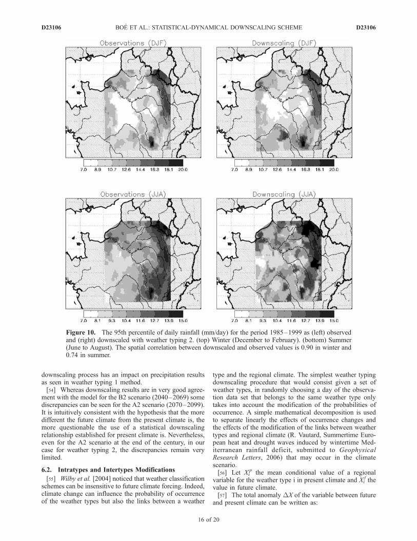
tation of the spatial variability of the regional climate isnecessary. Here, the SDMs are based on resampling strat-egies, which are known to provide a good way to deal withspatial variability issues. As anticipated, the downscaledARPEGE simulation with the weather typing 2 methodpresents a realistic representation of the spatial variabilityof mean rainfall amounts both in winter and summer asshown on Figure 9. The spatial variability of the 95thpercentile of daily downscaled rainfall in winter and sum-mer is also spatially close to the observations (Figure 10).[47] Figure 11 shows the Probability Density Function

(PDF) of rainfall and temperature as observed and down-scaled. Two grid points are considered, corresponding todifferent rainfall characteristics. The point A, characterizedby wet conditions, is located in the east of D2. The point Bis situated in the west of the domain and is characterized bydriest condition (see Figure 1 for the exact location of thepoints). Some minor discrepancies are seen. For the point Athe model slightly underestimates the probability to havedry conditions whereas it is the inverse for the point B.Concerning temperature, the shape of the PDF is well

Table 8. Linear Trend for the 90th Percentile of Minimum

Temperature in Summer (K by Decade), 1957–2002a

Station Observations Analog Weather Typing 1 Weather Typing 2

S11 0.28 0.02 0.10 0.19S4 0.41 0.05 0.20 0.26S15 0.31 0.05 0.20 0.33S6 0.36 �0.07 0.20 0.28S1 0.42 0.04 0.17 0.31S2 0.47 0.16 0.16 0.29S5 0.33 �0.04 0.11 0.21aThe values significant at the 0.05 level are presented in bold.

Table 9. Linear Trend for the 90th Percentile of Maximum

Temperature in Winter (K by Decade), 1957–2002a

Station Observations Analog Weather Typing 1 Weather Typing 2

S8 0.24 0.43 0.33 0.47S14 0.30 0.38 0.35 0.46S3 0.26 0.40 0.25 0.39S4 0.21 0.42 0.27 0.43S13 0.23 0.42 0.26 0.47S15 0.35 0.36 0.30 0.33S6 0.31 0.45 0.25 0.48S1 0.27 0.34 0.22 0.33S7 0.32 0.45 0.28 0.44S2 0.30 0.22 0.23 0.30aThe values significant at the 0.05 level are presented in bold.

D23106 BOE ET AL.: STATISTICAL-DYNAMICAL DOWNSCALING SCHEME

11 of 20

D23106

Figure 5. Mean and standard deviation of Z500 in (top) winter (December to February) and (bottom)summer (June to August) over the 1958–1999 period for (left) ERA40 and (right) the ARPEGE Model.Contour lines indicate mean (m). Shading indicates standard deviation (m).

Figure 6. Probability of occurrence of the weather types for each season (1961–1990): ERA40 (solid)versus ARPEGE (shaded).

D23106 BOE ET AL.: STATISTICAL-DYNAMICAL DOWNSCALING SCHEME

12 of 20

D23106

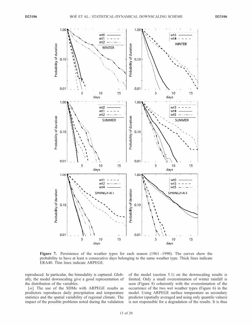
reproduced. In particular, the bimodality is captured. Glob-ally, the model downscaling give a good representation ofthe distribution of the variables.[48] The use of the SDMs with ARPEGE results as

predictors reproduces daily precipitation and temperaturestatistics and the spatial variability of regional climate. Theimpact of the possible problems noted during the validation

of the model (section 5.1) on the downscaling results islimited. Only a small overestimation of winter rainfall isseen (Figure 8) coherently with the overestimation of theoccurrence of the two wet weather types (Figure 6) in themodel. Using ARPEGE surface temperature as secondarypredictor (spatially averaged and using only quantile values)is not responsible for a degradation of the results. It is thus

Figure 7. Persistence of the weather types for each season (1961–1990). The curves show theprobability to have at least n consecutive days belonging to the same weather type. Thick lines indicateERA40. Thin lines indicate ARPEGE.

D23106 BOE ET AL.: STATISTICAL-DYNAMICAL DOWNSCALING SCHEME

13 of 20

D23106

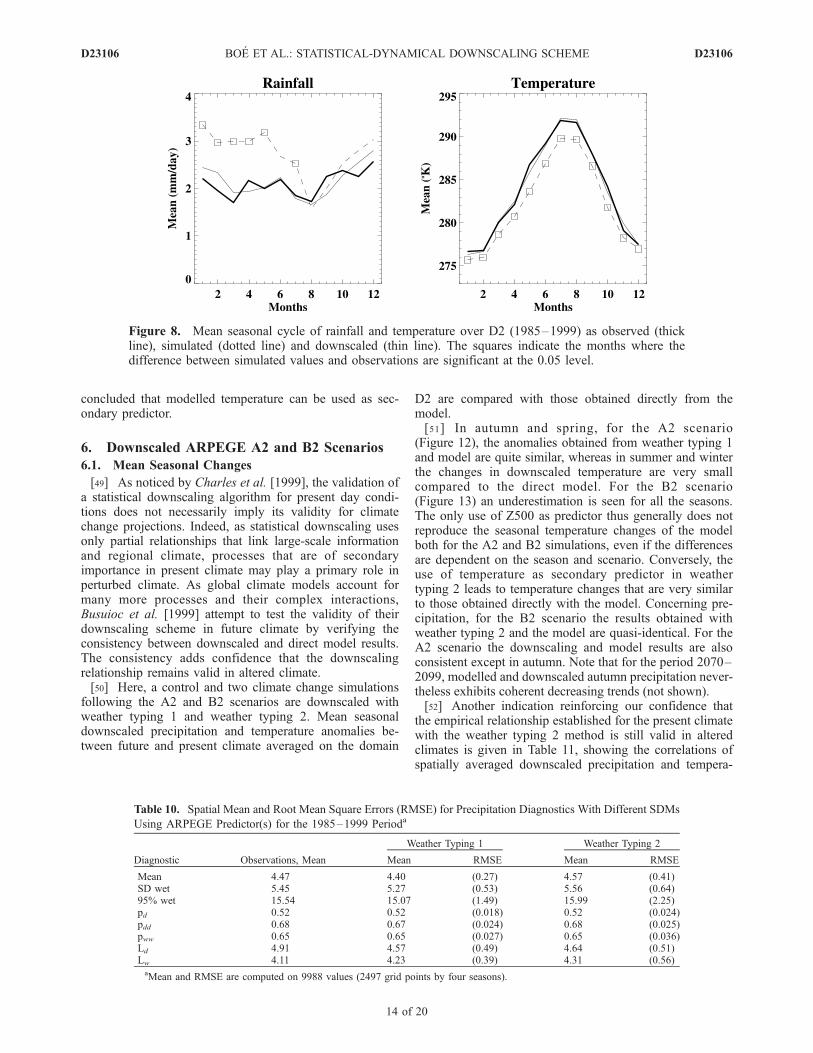
concluded that modelled temperature can be used as sec-ondary predictor.

6. Downscaled ARPEGE A2 and B2 Scenarios

6.1. Mean Seasonal Changes

[49] As noticed by Charles et al. [1999], the validation ofa statistical downscaling algorithm for present day condi-tions does not necessarily imply its validity for climatechange projections. Indeed, as statistical downscaling usesonly partial relationships that link large-scale informationand regional climate, processes that are of secondaryimportance in present climate may play a primary role inperturbed climate. As global climate models account formany more processes and their complex interactions,Busuioc et al. [1999] attempt to test the validity of theirdownscaling scheme in future climate by verifying theconsistency between downscaled and direct model results.The consistency adds confidence that the downscalingrelationship remains valid in altered climate.[50] Here, a control and two climate change simulations

following the A2 and B2 scenarios are downscaled withweather typing 1 and weather typing 2. Mean seasonaldownscaled precipitation and temperature anomalies be-tween future and present climate averaged on the domain

D2 are compared with those obtained directly from themodel.[51] In autumn and spring, for the A2 scenario

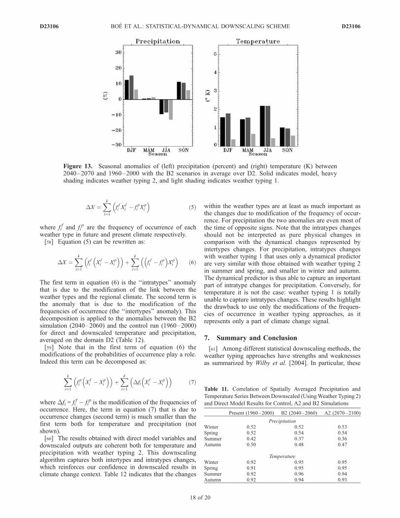
(Figure 12), the anomalies obtained from weather typing 1and model are quite similar, whereas in summer and winterthe changes in downscaled temperature are very smallcompared to the direct model. For the B2 scenario(Figure 13) an underestimation is seen for all the seasons.The only use of Z500 as predictor thus generally does notreproduce the seasonal temperature changes of the modelboth for the A2 and B2 simulations, even if the differencesare dependent on the season and scenario. Conversely, theuse of temperature as secondary predictor in weathertyping 2 leads to temperature changes that are very similarto those obtained directly with the model. Concerning pre-cipitation, for the B2 scenario the results obtained withweather typing 2 and the model are quasi-identical. For theA2 scenario the downscaling and model results are alsoconsistent except in autumn. Note that for the period 2070–2099, modelled and downscaled autumn precipitation never-theless exhibits coherent decreasing trends (not shown).[52] Another indication reinforcing our confidence that

the empirical relationship established for the present climatewith the weather typing 2 method is still valid in alteredclimates is given in Table 11, showing the correlations ofspatially averaged downscaled precipitation and tempera-

Figure 8. Mean seasonal cycle of rainfall and temperature over D2 (1985–1999) as observed (thickline), simulated (dotted line) and downscaled (thin line). The squares indicate the months where thedifference between simulated values and observations are significant at the 0.05 level.

Table 10. Spatial Mean and Root Mean Square Errors (RMSE) for Precipitation Diagnostics With Different SDMs

Using ARPEGE Predictor(s) for the 1985–1999 Perioda

Diagnostic Observations, Mean

Weather Typing 1 Weather Typing 2

Mean RMSE Mean RMSE

Mean 4.47 4.40 (0.27) 4.57 (0.41)SD wet 5.45 5.27 (0.53) 5.56 (0.64)95% wet 15.54 15.07 (1.49) 15.99 (2.25)pd 0.52 0.52 (0.018) 0.52 (0.024)pdd 0.68 0.67 (0.024) 0.68 (0.025)pww 0.65 0.65 (0.027) 0.65 (0.036)Ld 4.91 4.57 (0.49) 4.64 (0.51)Lw 4.11 4.23 (0.39) 4.31 (0.56)aMean and RMSE are computed on 9988 values (2497 grid points by four seasons).

D23106 BOE ET AL.: STATISTICAL-DYNAMICAL DOWNSCALING SCHEME

14 of 20

D23106

ture series with the direct model results. Even if a GCM failsto totally reproduce the small scale features of regionalclimate by construction, it should nevertheless partiallycapture the links between the large-scale climatic state andthe regional climate. Consequently, for present climate, asignificant correlation is found between the downscaledseries and the direct model results averaged on D2 fortemperature and precipitation in all seasons. It is theninteresting to note that the strength of this statistical linkis unchanged in future climate simulations for both scenar-ios with the weather typing 2 method. If a major modifica-tion (captured by the model) of the link between LSCpatterns and regional climate has occurred with climatechange, a net degradation of the correlation between down-scaled and direct model results would have been be noted. Itis not the case for weather typing 2. For weather typing 1,an important diminution of the correlation for temperature isnoted (not shown).

[53] In summary, our results give confidence in the use ofthe weather typing 2 SDM for climate change studies.Conversely it is concluded that weather typing 1 is notapplicable to altered climates. Downscaling based onlyupon LSC predictors does not correctly represent tempera-ture changes and even, to a lesser extent precipitationmodifications. Differences are noticed between weathertyping 1 and weather typing 2 results concerning precipita-tion. As these two methods only differ by the use of modeltemperature as secondary predictor in weather typing 2, thismight underline the role of temperature changes in precip-itation modifications. The relative change in water-holdingcapacity of the atmosphere is governed by the Clausius-Clapeyron equation and is therefore approximately propor-tional to temperature change. As the models suggest that thechanges in relative humidity are small, the moisture contentshould vary proportionally to temperature changes[Trenberth et al., 2003]. Even if the interactions betweenhumidity modifications and precipitation are complex,the misrepresentation of temperature changes through

Figure 9. Rainfall climatologies (1985–1999) as (left) observed and (right) downscaled with weathertyping 2 (mm/day). (top) Winter (December to February). (bottom) Summer (June to August). The spatialcorrelation between downscaled and observed fields is 0.91 in winter and 0.90 in summer.

D23106 BOE ET AL.: STATISTICAL-DYNAMICAL DOWNSCALING SCHEME

15 of 20

D23106

downscaling process has an impact on precipitation resultsas seen in weather typing 1 method.[54] Whereas downscaling results are in very good agree-

ment with the model for the B2 scenario (2040–2069) somediscrepancies can be seen for the A2 scenario (2070–2099).It is intuitively consistent with the hypothesis that the moredifferent the future climate from the present climate is, themore questionable the use of a statistical downscalingrelationship established for present climate is. Nevertheless,even for the A2 scenario at the end of the century, in ourcase for weather typing 2, the discrepancies remain verylimited.

6.2. Intratypes and Intertypes Modifications

[55] Wilby et al. [2004] noticed that weather classificationschemes can be insensitive to future climate forcing. Indeed,climate change can influence the probability of occurrenceof the weather types but also the links between a weather

type and the regional climate. The simplest weather typingdownscaling procedure that would consist given a set ofweather types, in randomly choosing a day of the observa-tion data set that belongs to the same weather type onlytakes into account the modification of the probabilities ofoccurrence. A simple mathematical decomposition is usedto separate linearly the effects of occurrence changes andthe effects of the modification of the links between weathertypes and regional climate (R. Vautard, Summertime Euro-pean heat and drought waves induced by wintertime Med-iterranean rainfall deficit, submitted to GeophysicalResearch Letters, 2006) that may occur in the climatescenario.[56] Let Xi

p the mean conditional value of a regionalvariable for the weather type i in present climate and Xi

f thevalue in future climate.[57] The total anomaly DX of the variable between future

and present climate can be written as:

Figure 10. The 95th percentile of daily rainfall (mm/day) for the period 1985–1999 as (left) observedand (right) downscaled with weather typing 2. (top) Winter (December to February). (bottom) Summer(June to August). The spatial correlation between downscaled and observed values is 0.90 in winter and0.74 in summer.

D23106 BOE ET AL.: STATISTICAL-DYNAMICAL DOWNSCALING SCHEME

16 of 20

D23106

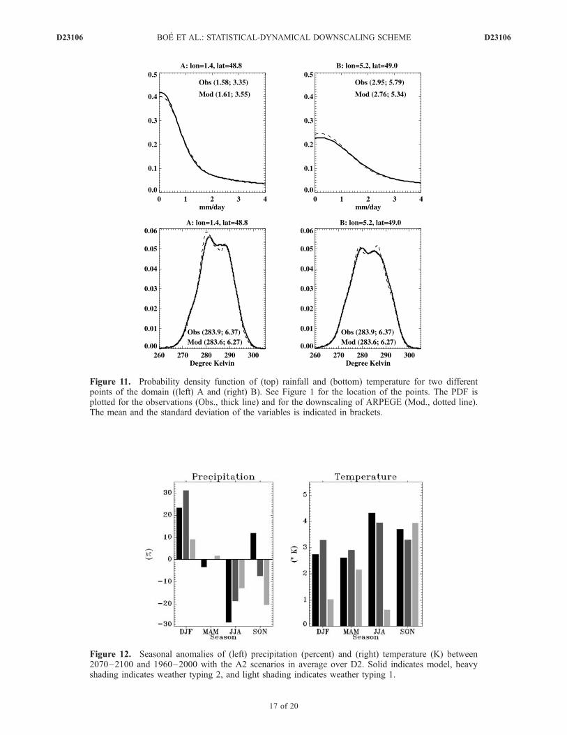
Figure 11. Probability density function of (top) rainfall and (bottom) temperature for two differentpoints of the domain ((left) A and (right) B). See Figure 1 for the location of the points. The PDF isplotted for the observations (Obs., thick line) and for the downscaling of ARPEGE (Mod., dotted line).The mean and the standard deviation of the variables is indicated in brackets.

Figure 12. Seasonal anomalies of (left) precipitation (percent) and (right) temperature (K) between2070–2100 and 1960–2000 with the A2 scenarios in average over D2. Solid indicates model, heavyshading indicates weather typing 2, and light shading indicates weather typing 1.

D23106 BOE ET AL.: STATISTICAL-DYNAMICAL DOWNSCALING SCHEME

17 of 20

D23106

DX ¼Xki¼1

ffi X

fi � f

pi X

pi

� �ð5Þ

where fif and fi

p are the frequency of occurrence of eachweather type in future and present climate respectively.[58] Equation (5) can be rewritten as:

DX ¼Xki¼1

ffi X

fi � X

pi

� �� �þXki¼1

ffi � f

pi

� �X

pi

� �ð6Þ

The first term in equation (6) is the ‘‘intratypes’’ anomalythat is due to the modification of the link between theweather types and the regional climate. The second term isthe anomaly that is due to the modification of thefrequencies of occurrence (the ‘‘intertypes’’ anomaly). Thisdecomposition is applied to the anomalies between the B2simulation (2040–2060) and the control run (1960–2000)for direct and downscaled temperature and precipitation,averaged on the domain D2 (Table 12).[59] Note that in the first term of equation (6) the

modifications of the probabilities of occurrence play a role.Indeed this term can be decomposed as:

Xki¼1

fpi X

fi � X

pi

� �� �þXki¼1

Dfi Xfi � X

pi

� �� �ð7Þ

where Dfi = fif � fi

p is the modification of the frequencies ofoccurrence. Here, the term in equation (7) that is due tooccurrence changes (second term) is much smaller than thefirst term both for temperature and precipitation (notshown).[60] The results obtained with direct model variables and

downscaled outputs are coherent both for temperature andprecipitation with weather typing 2. This downscalingalgorithm captures both intertypes and intratypes changes,which reinforces our confidence in downscaled results inclimate change context. Table 12 indicates that the changes

within the weather types are at least as much important asthe changes due to modification of the frequency of occur-rence. For precipitation the two anomalies are even most ofthe time of opposite signs. Note that the intratypes changesshould not be interpreted as pure physical changes incomparison with the dynamical changes represented byintertypes changes. For precipitation, intratypes changeswith weather typing 1 that uses only a dynamical predictorare very similar with those obtained with weather typing 2in summer and spring, and smaller in winter and autumn.The dynamical predictor is thus able to capture an importantpart of intratype changes for precipitation. Conversely, fortemperature it is not the case: weather typing 1 is totallyunable to capture intratypes changes. These results highlightthe drawback to use only the modifications of the frequen-cies of occurrence in weather typing approaches, as itrepresents only a part of climate change signal.

7. Summary and Conclusion

[61] Among different statistical downscaling methods, theweather typing approaches have strengths and weaknessesas summarized by Wilby et al. [2004]. In particular, these

Figure 13. Seasonal anomalies of (left) precipitation (percent) and (right) temperature (K) between2040–2070 and 1960–2000 with the B2 scenarios in average over D2. Solid indicates model, heavyshading indicates weather typing 2, and light shading indicates weather typing 1.

Table 11. Correlation of Spatially Averaged Precipitation and

Temperature Series Between Downscaled (UsingWeather Typing 2)

and Direct Model Results for Control, A2 and B2 Simulations

Present (1960–2000) B2 (2040–2060) A2 (2070–2100)

PrecipitationWinter 0.52 0.52 0.53Spring 0.52 0.54 0.54Summer 0.42 0.37 0.36Autumn 0.50 0.48 0.47

TemperatureWinter 0.92 0.95 0.95Spring 0.91 0.95 0.95Summer 0.92 0.96 0.94Autumn 0.92 0.94 0.93

D23106 BOE ET AL.: STATISTICAL-DYNAMICAL DOWNSCALING SCHEME

18 of 20

D23106

methods yield physically interpretable linkages to surfaceclimate and can be applied to a wide range of problems.Nevertheless they require additional task of weather classi-fication and can be insensitive to future climate forcing. Inparticular they may not capture intratype variations insurface climate. In this study, a simple yet efficient weathertyping-based methodology intended to overcome theseweaknesses is developed.[62] A bottom-up approach starting from regional climate

properties to establish discriminating weather types for localvariables is applied. To take into account the intratypevariations in surface climate, the distances to the weathertypes are then used in the downscaling process. Theperformance of the weather typing methods is tested againsta standard analog approach, considered as a natural ‘‘bench-mark’’ method, as it has proven to be both simple andskillful (Zorita and von Storch [1999]). The major advan-tages of weather typing compared to analogs is the possiblestudy of the physical mechanisms on which the statisticaldownscaling is based.[63] First, using ERA40 reanalysis fields as predictors

(z500 for weather typing 1, z500 and surface temperaturefor weather typing 2), it was shown that the weather typingmethod developed in this paper is superior to the standardanalog method and successfully reproduces daily statisticproperties of precipitation. Moreover, low-frequency varia-tions of downscaled temperature and precipitation are wellsimulated and close to the observations. Next, the weathertyping methods were tested using as predictors the results ofa global GCM simulation with high resolution over thestudy area thanks to a variable resolution. As the atmo-spheric circulation is globally well reproduced in the GCM,when applying the SDMs, a good representation of regionalclimate properties is obtained. The model temperature canbe used as secondary predictor without loss of performance,even if temperature is globally underestimated by the modelbecause of the way it is used within the downscalingprocess. It is worth noting that even with high resolutionover the study area the model has important biases for meantemperature and precipitation. Using statistical downscalingprovides an important improvement of the results.

[64] The consistency of downscaling and raw modelresults are tested for two future climate simulations. Theweather typing method that uses temperature as a secondarypredictor yields results that are consistent with modelchanges both for temperature and precipitation with theB2 scenario. With the A2 scenario the results are alsoconsistent except in autumn for precipitation. These resultsgive confidence in the use of this SDM for climate changeapplications. Conversely, if the temperature is not used assecondary predictor, the SDM fails to reproduce the tem-perature changes and in a lesser extent the precipitationchanges. The latter is considered not applicable in alteredclimates. By contrast, this SDM correctly reproduces pres-ent day regional climate. As in Charles et al. [1999], theseresults highlight the importance of evaluating the plausibil-ity of climate change projections on the basis of statisticaldownscaling.[65] The SDMs used in this study are based on a

resampling strategy. The major weakness of this approachis that resampling is incapable of giving values outside thealready observed range of values. This drawback is com-mon to many SDM, as resampling strategies are oftenchosen when dealing with spatial and multivariate prob-lems. It is the case for the weather typing and analogmethods, and also when single-site results are extended tomultiple sites from regression-based methods [Wilby et al.,2003] or weather generators [Palutikof et al., 2002]. Forhydrological applications, as the greatest present day cumu-lated amount of precipitation over N days can be exceeded,the greatest streamflow of present climate can also beexceeded in future climate. Depending upon the character-istics of the watershed, the limitation of resampling strate-gies concerning the extreme values is more or lessimportant. It must also be noted that in the A2 scenariofor the whole 2070–2100 period, the greatest value of meanprecipitation on the domain D2 in the control run (1960–2000) is only exceeded for 16 days. This thus reinforces ourconfidence in the use of a resampling strategy for thedownscaling of the Seine basin precipitation. Nevertheless,generally, when analyzing the results of climate changeimpact assessments obtained by SDM on the basis ofresampling this point should be carefully considered.[66] Finally it is concluded that the downscaling method-

ology developed in this paper can be applied to the study ofthe impacts of climate change on the Seine basin hydrology,which will be the object of a future study. This method mayalso find other applications, as for example seasonal hydro-logical forecast.

[67] Acknowledgments. This work was supported by the ProgrammeNational de Recherche en Hydrologie (PNRH) under the RIVAGES projectand by the European Community via the sixth framework programENSEMBLES project under contract GOCE-CT-2003-505539. ECMWFERA-40 data used in this study have been obtained from the ECMWF dataserver. The authors are grateful to the Division de la Climatologie (DCLIM)at Meteo-France for providing the SQR data set. They would like to thankM. Deque for providing the PRUDENCE simulations and C. Cassou forstimulating discussion about this work.

ReferencesAllen, M. R., and W. J. Ingram (2002), Constraints on future changes inclimate and the hydrologic cycle, Nature, 419, 224–232.

Bengtsson, L., S. Hagemann, and K. I. Hodges (2004), Can climate trendsbe calculated from reanalysis data?, J. Geophys. Res., 109, D11111,doi:10.1029/2004JD004536.

Table 12. Decomposition of the Temperature and Precipitation

Seasonal Anomalies Averaged on the Domain D2 Between the B2

Simulation (2040–2060) and the Control Run (1960–2000) for

Direct Model and Downscaled Results With Weather Typing 2a

Model Downscaling

Intertypes Intratypes Intertypes Intratypes

Precipitation, mm/dayDJF �0.03 0.38 0.06 0.26 (0.10)MAM �0.31 0.37 �0.34 0.38 (0.39)JJA �0.41 0.21 �0.72 0.45 (0.44)SON �0.17 0.38 �0.24 0.47 (0.36)

Temperature, KDJF 0.16 1.37 0.24 1.54 (0.11)MAM 0.73 0.67 0.86 0.72 (�0.32)JJA 0.84 1.32 0.89 1.32 (�0.49)SON 0.45 0.41 0.44 0.52 (0.12)

aFor intratypes changes results obtained with weather typing 1 are alsoshown in brackets (the intertypes changes are quasi-identical with the twomethods). See text for calculation explanation.

D23106 BOE ET AL.: STATISTICAL-DYNAMICAL DOWNSCALING SCHEME

19 of 20

D23106

Busuioc, A., H. von Storch, and R. Schnur (1999), Verification of GCM-generated regional seasonal precipitation for current climate and of sta-tistical downscaling estimates under changing climate conditions,J. Clim., 12(1), 258–272.

Cassou, C., L. Terray, and A. S. Phillips (2005), Tropical Atlantic influenceon European heatwaves, J. Clim., 18(15), 2805–2811.

Charles, S. P., B. C. Bates, P. H. Whetton, and J. P. Hugues (1999), Valida-tion of downscaling models for changes climate conditions: Case study ofsouthwestern Australia, Clim. Res., 12, 1–14.

Corte-Real, J., B. Qian, and H. Xu (1999), Circulation patterns, daily pre-cipitation in Portugal and implications for climate change simulated bythe second Hadley Centre GCM, Clim. Dyn., 15, 921–935.

Durand, Y., E. Brun, L. Merindol, G. Guyomarc’h, B. Lesaffre, andE. Martin (1993), A meteorological estimation of relevant parameters forsnow schemes used with atmospheric models, Ann. Glaciol., 18, 65–71.

Ebisuzaki, W. (1997), A method to estimate the statistical significance of acorrelation when the data are serially correlated, J. Clim., 10(9), 2147–2153.

Etchevers, P., C. Golaz, F. Habets, and J. Noilhan (2002), Impact of aclimate change on the Rhone river catchment hydrology, J. Geophys.Res., 107(D16), 4293, doi:10.1029/2001JD000490.

Gibelin, A.-L., and M. Deque (2003), Anthropogenic climate changeover the Mediterranean region simulated by a global variable resolutionmodel, Clim. Dyn., 20, 327–339.

Giorgi, F., M. R. Marinucci, and G. Visconti (1990), Use of a limited-areamodel nested in a general circulation model for regional climate simula-tion over Europe, J. Geophys. Res., 95(D11), 18,413–18,431.

Gutierrez, J. M., A. S. Cofino, R. Cano, and M. A. Rodrıguez (2004),Clustering methods for statistical downscaling in short-range weatherforecast, Mon. Weather Rev., 132(9), 2169–2183.

Habets, F., P. Etchevers, C. Golaz, E. Leblois, E. Ledoux, E. Martin,J. Noilhan, and C. Ottle (1999), Simulation of the water budgetand the river flows of the Rhone basin, J. Geophys. Res.,104(D24), 31,145–31,172.

Jones, T. C., et al. (2003), Anthropogenic climate change for 1860 to 2100simulated with the HadCM3 model under updated emission scenarios,Clim. Dyn., 20, 583–612.

Klein Tank, A. M. G., and G. P. Konnen (2003), Trends in indices of dailytemperature and precipitation extremes in Europe, 1946–99, J. Clim.,16(22), 3665–3680.

Ledoux, E., G. Girard, and J. P. Villeneuve (1984), Proposition d’un modelecouple pour la simulation conjointe des ecoulements de surface et desecoulements souterrains sur un bassin hydrologique, Houille Blanche,1/2-1984, 101–110.

Martin, E., B. Timbal, and E. Brun (1997), Downscaling of general circula-tion model outputs: Simulation of the snow climatology of the FrenchAlps and sensitivity to climate change, Clim. Dyn., 13, 45–56.

Mearns, L. O., I. Bogardi, F. Giorgi, I. Matyasovszky, and M. Palecki(1999), Comparison of climate change scenarios generated from regionalclimate model experiments and statistical downscaling, J. Geophys. Res.,104(D6), 6603–6621.

Mehrotra, R., and A. Sharma (2005), A nonparametric nonhomogeneoushidden Markov model for downscaling of multisite daily rainfall occur-ences, J. Geophys. Res., 110, D16108, doi:10.1029/2004JD005677.

Michelangeli, P.-A., R. Vautard, and B. Legras (1995), Weather regimes:Recurrence and quasi stationarity, J. Atmos. Sci., 52(8), 1237–1256.

Moisselin, J. M., M. Schneider, C. Canellas, and O. Mestre (2002), Chan-gements climatiques en France au 20eme siecle. Etude des longues seriesde donnees homogeneises francaises de precipitations et temperatures,Meteorologie, 38, 45–46.

Noilhan, J., and S. Planton (1989), A simple parametrization of land surfaceprocesses for meteorological models, Mon. Weather Rev., 117, 536–549.

Palutikof, J. P., C. M. Goodess, S. J. Watkins, and T. Holt (2002), Generat-ing rainfall and temperature scenarios at multiple sites: Examples fromthe Mediterranean, J. Clim., 15(24), 3529–3548.

Plaut, G. (2004), Building downscaling algorithms for precipitation: The‘‘Potential Precipitation Circulation Index’’or ‘‘ppci’’, an adaptive pre-dictor to downscale extreme precipitation on the french Alpes Maritimes,STARDEX project partner 5 (CNRS-INLN) report for deliverable D10,Clim. Res. Unit, Univ. of East Anglia, Norwich, U.K. (Available http://www.cru.uea.ac.uk/cru/projects/stardex/deliverables/D10/)

Plaut, G., E. Schuepbach, and M. Doctor (2001), Heavy precipitation eventsover a few Alpine sub-regions and the links with large-scale circulation,1971–1995, Clim. Res., 17, 285–302.

Roebber, P. J., and L. F. Bosart (1998), The sensitivity of precipitation tocirculation details. Part I: An analysis of regional analogs, Mon. WeatherRev., 126, 437–455.

Royer, J. F., et al. (2002), Simulation of climate changes during the 21stcentury including stratospheric ozone, C. R. Geosci., 334, 147–154.

Schubert, S. (1998), Downscaling local extreme temperature changes insouth-eastern Australia from the CSIRO MARK2 GCM, Int. J. Climatol.,18, 1419–1438.

Straus, D. M., and F. Molteni (2004), Circulation regimes and SST forcings:Results from large GCM ensembles, J. Clim., 17(8), 1641–1656.

Terray, L., M.-E. Demory, M. Deque, G. de Coetlogon, and E. Maisonnave(2004), Simulation of late-twenty-first-century changes in wintertime at-mospheric circulation over Europe due to anthropogenic causes, J. Clim.,17(24), 4630–4635.

Timbal, B. (2004), Southwest Australia past and future rainfall trends, Clim.Res., 26(3), 233–249.

Timbal, B., A. Dufour, and B. McAvaney (2003), An estimate of futureclimate change for western France using a statistical downscaling tech-nique, Clim. Dyn., 20, 807–823.

Trenberth, K. E., A. Dai, R. M. Rasmussen, and D. B. Parsons (2003), Thechanging character of precipitation, Bull. Am. Meteorol. Soc, 84, 1205–1217.

von Storch, H. (1999), On the use of ‘‘inflation’’ in statistical downscaling,J. Clim., 12(12), 3505–3506.

Wilby, R. L., T. M. L. Wigley, D. Conway, P. D. Jones, B. C. Hewitson,J. Main, and D. S. Wilks (1998), Statistical downscaling of generalcirculation model output: A comparison of methods, Water Resour.Res., 34(11), 2995–3008.

Wilby, R. L., O. J. Tomlinson, and C. W. Dawson (2003), Multi-site simu-lation of precipitation by conditional resampling, Clim. Res., 23, 183–194.

Wilby, R. L., S. P. Charles, E. Zorita, B. Timbal, P. Whetton, and L. O.Mearns (2004), Guidelines for use of climate scenarios developed fromstatistical downscaling methods, Data Distrib. Cent. of the Intergovt.Panel on Clim. Change, Geneva, Switzerland.

Wilson, L. L., D. P. Lettenmaier, and E. Skyllingstad (1992), A hierarchicalstochastic model of large-scale atmospheric circulation patterns and mul-tiple station daily precipitation, J. Geophys. Res., 97(D3), 2791–2809.

Zhang, X., X. Wang, and J. Corte-Real (1997), On the relationships be-tween daily circulation patterns and precipitation in Portugal, J. Geophys.Res., 102(D12), 13,495–13,507.

Zorita, E., and H. von Storch (1999), The analog method as a simplestatistical downscaling technique: comparison with more complicatedmethods, J. Clim., 12(8), 2474–2489.

Zorita, E., J. P. Hughes, D. P. Lettemaier, and H. von Storch (1995), Sto-chastic characterization of regional circulation patterns for climate modeldiagnosis and estimation of local precipitation, J. Clim., 8(5), 1023–1042.

�����������������������J. Boe and L. Terray, Climate Modelling and Global Change Team,

CERFACS/CNRS, SUC URA1875, 42 Avenue Gaspard Coriolis, F-31057,Toulouse Cedex 1, France. ([email protected])F. Habets and E. Martin, Centre National de Recherches Meteorologi-

ques, Meteo-France, F-31057 Toulouse, France.

D23106 BOE ET AL.: STATISTICAL-DYNAMICAL DOWNSCALING SCHEME

20 of 20

D23106