A simple predatorâ€“prey model of exploited marine fish populations

ICES Journal of Marine Science, 53: 615–628. 1995

A simple predator–prey model of exploited marine fishpopulations incorporating alternative prey

Paul D. Spencer and Jeremy S. Collie

Spencer, P. D. and Collie, J. S. 1996. A simple predator–prey model of exploitedmarine fish populations incorporating alternative prey. – ICES Journal of MarineScience, 53: 615–628.

A simple two-species population model in which the predator is partially coupled tothe prey is developed. The model is an extension of traditional two-species models butless complex than a three-species system. The growth rate of the predator dependsupon predation on the modeled and alternate prey; this formulation provides greaterrealism in describing marine piscivores, such as spiny dogfish (Squalus acanthias), thantwo-species predator–prey models. Two stable equilibria separated by a saddle pointpotentially exist for the predator–prey system, and stochastic variability can lead tomovement between equilibrium abundance levels. In addition, endogenous limit cyclesmay exist in the presence of predator fishing mortality. The model is applied to thepredation of spiny dogfish on a representative groundfish species, the Georges Bankhaddock (Melanogrammus aeglefinus). Stochastic variability is input to the model inthe form of ‘‘red noise’’ (variance is a decreasing function of frequency), a featureobserved in marine environments. Predator abundance can increase when the modeledprey abundance is low, due to consumption of alternate prey, consistent with thepattern observed in the spiny dogfish–haddock abundances. Increased harvesting onthe predator species allows the prey species to spend a greater proportion of time at thehigh equilibrium. The model presented here poses the interesting management problemof finding the optimal combination of fishing mortality rates for the two species.

? 1996 International Council for the Exploration of the Sea

Key words: predator–prey model, autocorrelated variability, functional response,marine fisheries, exploitation, management.

Received 15 February 1995; accepted 20 October 1995

P. D. Spencer and J. S. Collie: University of Rhode Island, Graduate School ofOceanography, Narragansett, Rhode Island, USA, 02882.

Introduction

A characteristic feature of marine fish populations isdramatic changes in abundance over decadal time scales.A review by Caddy and Gulland (1983) indicated thatexploited populations can be classified as ‘‘steady, cyclic,irregular or spasmodic’’, with no exact criteria for theboundaries between groups. Because the management ofmarine fisheries is complicated greatly by populationfluctuations, the identification of causes of non-equilibrium behavior is of significant practical impor-tance. Early fisheries models assumed a single-speciesequilibrium view, in which temporal changes in popu-lation size are caused by corresponding changes inexploitation (Schaefer, 1954). (‘‘Equilibrium’’ is definedhere as a fixed point which a population is very closelyassociated with; any slight perturbation in populationsize is countered by compensatory biotic interactions. Incontrast, ‘‘non-equilibrium’’ refers to systems which

show little association with specific fixed points.) Datafrom scale deposits in anaerobic sediments, however,indicate that population fluctuations can occur in theabsence of exploitation (Soutar and Isaacs, 1974), andan ongoing debate in fisheries science is ascertaining therelative importance of exploitation and environmentalfactors in determining population levels.The effect of environmental variability on populations

depends on its time scale (ô) relative to the characteristicresponse time of the population (Tr, the ‘‘speed’’ atwhich a population returns to equilibrium once dis-turbed), and in marine systems it is reasonable to expectenvironmental variability to produce non-equilibriumfluctuations. Relatively short-term changes in environ-mental conditions can be viewed as affecting populationsprimarily through changes in growth rate, whereaspersistent, long-term changes may affect equilibriumpopulation levels (Pimm, 1984, Ch. 3). The latter case ispertinent to marine systems, where variability is a

1054–3139/96/030615+14 $18.00/0 ? 1996 International Council for the Exploration of the Sea

Dow

nloaded from https://academ

ic.oup.com/icesjm

s/article/53/3/615/625714 by guest on 01 Decem

ber 2021

decreasing function of frequency (‘‘red noise’’) and thushas important low frequency components (Steele, 1985).The effects of persistent changes in equilibria have beenillustrated by introducing cyclic change to the carryingcapacity, K, of the logistic model; when ô°Tr thepopulation dynamics will tend to smooth out the effectsof variability whereas when ô±Tr, the populationdynamics will be driven by environmental variability(May, 1976). Environmental variability can thus sub-stantially affect marine ecosystems where the Tr ofmany organisms is less than ô (Steele, 1985). Steele andHenderson (1984) showed that a commonly used single-species model can ‘‘flip’’ between multiple stableequilibria when forced with red noise. Similarly, atwo-species, predator–prey model forced with red noisewas used to describe the dynamics of Pacific herring(Clupea pallasi) preyed on by Pacific hake (Merlucciusproductus) (Collie and Spencer, 1994).Compensatory biotic interactions are likely to exist in

marine communities, although they are often obscuredby environmental variability. In particular, predation isbelieved to play a major role in the community structureof marine fish; for example, in the north-west Atlanticthe importance of predation by spiny dogfish (Squalusacanthias) in structuring the Georges Bank fish com-munity is becoming increasingly recognized (Overholtzet al., 1991). Thus, harvesting may affect entire com-munities via species interactions, although the modelscurrently being used for management purposes arepredominantly single-species approaches. In addition,many marine piscivores, including spiny dogfish in thenorth-west Atlantic and Pacific hake, undertake exten-sive seasonal migrations on a spatial scale much largerthan the habitat occupied by some of their prey, and thedevelopment of realistic models for these predator–preysystems will require consideration of alternate prey.Early predator–prey models have focused on one-

predator, one-prey systems, and the dynamics of thesemodels are well known. More recent theoretical modelshave considered additional trophic levels (Abrams andRoth, 1994) and alternate prey (Vance, 1978). Addition-ally, many investigators have moved from traditionalmodels with clear equilibria to non-equilibrium modelsthat focus on the persistence of communities; popu-lations may be unstable at small, ‘‘patch’’ scales, butmovement between ‘‘patches’’ may provide persis-tence at larger, ‘‘landscape’’ scales (DeAngelis andWaterhouse, 1987). Unfortunately, these developmentshave not provided a rigorous correspondence betweentheory and observations of real ecological systems(Kareiva, 1989). Determining the appropriate level ofdetail is critical for applied work; as one considers three(or more) species, the inherent complexity may precludeany rigorous application to field data (May, 1977).Spatially explicit models are of interest in a variety ofresource management applications (Dunning et al.,

1995), but the required additional knowledge of disper-sal and movement rates makes their validation difficult(Conroy et al., 1995). On large spatial scales, whichare usually of interest in marine fisheries management,simplified, traditional models may serve as usefulapproximations to system dynamics (DeAngelis andWaterhouse, 1987).Most applications of predator–prey models to marine

fisheries have been age-structured because predation isgenerally age- or size-dependent. Andersen and Ursin’s(1977) ecosystem model of the North Sea has evolvedinto what is known as Multispecies Virtual PopulationAnalysis (MSVPA, Sparre, 1991). This multispeciesanalysis reconstructs the abundance of each cohort,accounting for the observed feeding interactionsbetween species. The goal of MSVPA has been primarilyto improve stock assessment and to estimate predationrates and feeding preference functions. Combined withassumptions about recruitment, the feeding preferencemodel can be simulated forward in time to providemedium-term management advice (Gislason, 1991). Upto 11 species have been included in MSVPA, but endog-enous dynamics (cycles, chaos) generally do not occurwhen predation and recruitment are not modeled withstrongly nonlinear functions. Attempts to link age-structured and age-aggregated models include introduc-ing density-dependent recruitment into age-structuredmodels (Overholtz et al., 1991), or constructing pro-duction models with the output of MSVPA (Blinov,1991).In this study, we develop a simple, two-species

predator–prey model that incorporates the effect ofalternative prey. Because our intent is to understand thedynamics of specific predator–prey systems, the model isdeliberately kept simple; it is an extension of traditionaltwo-species models but less complex than a three-speciessystem. First, the theoretical development of the modelwill be discussed, and the effects of harvesting either orboth of the predator–prey species will be examined.Second, realistic parameter values will be used to applythe model to the spiny dogfish–Georges Bank ground-fish interaction, and stochastic simulations will be run byforcing the model with a range of variability typical ofmarine environments.

Predator–prey model developmentA class of models describing populations experiencingpredation, reviewed by May (1977), is helpful in describ-ing dramatic fluctuations in abundance. A commonexample is a logistic production function combined witha sigmoidal type III predator functional response(Holling, 1965), leading to the presence of multipleequilibrium population levels. Continuous changes inthe intrinsic growth rate, carrying capacity, or rate ofpredation can lead to discontinuous bifurcations in

616 P. D. Spencer and J. S. Collie

Dow


ic.oup.com/icesjm


ber 2021

population size. Models of this form have been used todescribe the dynamics of grazed vegetation (Noy-Meir,1975) and the spruce budworm (Ludwig et al., 1978).Steele and Henderson (1984) have shown these modelsto be relevant to marine fishery systems. The modelformulation is

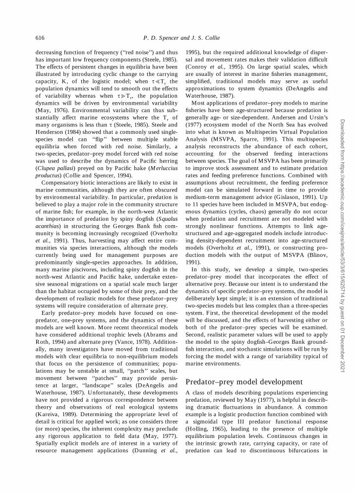
where P is the prey population size, r is an intrinsicgrowth rate, K is carrying capacity, C is a consumptionrate reflecting predator abundance (i.e. C=cH, where cis the per capita consumption rate and H is predatorabundance), and A is the prey abundance where pred-ator satiation begins. The location of equilibria can beseen graphically by plotting the prey and predatorisoclines (defined where dP/dt=0 and dH/dt=0, respec-tively) in the predator–prey phase space. The systemequilibria exist where the predator and prey isoclinesintersect; certain combinations of parameter valuesresult in three equilibria (referred to as the triple-valueregion (TVR)), with the outermost equilibria beingstable and the central equilibrium point being unstable(Fig. 1a). Either a single high or low equilibrium canoccur with different combinations of parameter values.The predator dynamics are not explicitly considered inthis system as H is assumed constant, leading to ahorizontal predator isocline. This situation occurs if theprey are an insignificant portion of the predators’ dietand thus the predator abundance is independent of preyabundance, although predation is clearly important inprey dynamics.The opposite limiting case describes situations in

which the predator consume only the modeled prey.Steele and Henderson (1981) extended system (1) byexplicitly including the predator dynamics:

where e is the conversion of prey biomass to predatorbiomass (thus, ec is the intrinsic growth rate of thepredator) and D is a quadratic closure coefficient. Ithas been shown that a linear form (DH) leads to un-stable equilibria and limit cycles (Rosenzweig, 1971)and is inappropriate for marine plankton (Steele andHenderson, 1992). Of several possible alternatives, theform DH2 is used here as the most economical inparameters. It can be regarded, formally, as applying alogistic closure for H (Getz, 1984). In contrast to system(1), the predator isocline is now constrained to passthrough the origin of the predator–prey phase space;when prey abundance is zero, the equilibrium predatorabundance is also zero (Fig. 1b). Note that different

values of the predator closure term D can also lead tosingle-equilibrium solutions, with high (or low) values ofD resulting in high (or low) equilibrium prey abundance.Local stability analysis (May, 1974) was used to cor-roborate the graphical approach (Fig. 1b) and to verifythat the unstable equilibrium of the TVR is a saddlepoint. Because the predator isocline is forced to passthrough the origin, extreme reductions in D do not resultin extreme increases in predator abundance (Fig. 1b).Instead, the lower equilibrium point is determinedlargely by the prey abundance at which satiation occurs,and reductions in D have relatively minor effects at lowprey abundances. This system was used to describeclosed experimental enclosures in which an aggregategroup of zooplankton fed upon an aggregate group ofphytoplankton (Steele and Henderson, 1981). Becausethe type III functional response is common amongvertebrates (Holling, 1965), this general predator–preyinteraction can be expected to occur at higher trophiclevels, as in the Pacific hake–Pacific herring interaction(Collie and Spencer, 1994).

Prey abundance

Pre

dato

r ab

un

dan

ce

High D

Low D (c)P

reda

tor

abu

nda

nce

High D

Low D(b)

Pre

dato

r ab

un

dan

ce

High C

(a)

Low C

Figure 1. Predator (dotted lines) and prey (solid lines) isoclinesfor (a) single-species model of Steele and Henderson (1984),(b) two-species model of Steele and Henderson (1981), and(c) two-species model developed in this study with F1=F2=0and 0<B<1. Stable (,) or unstable (#) equilibria occur wherethe isoclines intersect.

617A predator–prey model incorporating alternative prey

Dow


ic.oup.com/icesjm


ber 2021

Intermediate to the two limiting cases above is thesituation in which the predator dynamics are partiallycoupled to any particular prey species. The sigmoidalpredator response was derived by Holling (1965) inexperiments where the animals (mice preying on sawflylarvae) had an alternative but less preferred food source(broken biscuits). Feeding upon multiple prey seemsappropriate for fish which are predators on the larvaeand juveniles of numerous fish species and have alterna-tive sources of relatively abundant food. Thus, thegrowth rate of the predator should be maximal when P isabundant but non-zero when P]0. Consumption ofmultiple prey could occur over short time and spacescales or could be the result of seasonal migrations, orsome combination.System (2) can be modified to describe a partially

coupled predator–prey interaction:

The fishing mortality rates F1 and F2 are added to allowthe model to correspond to exploited fish populations;the effect of harvesting will be considered in the follow-ing section. The dimensionless parameter B representsthe degree of coupling between the predator andmodeled prey species. If B=1 the predator feeds onlyupon the modeled prey species and thus it is clear thatsystem (2) is a special case of system (3). Setting B=0corresponds to the two populations not interacting andthe growth rate of the predator is determined by preyoutside the two-species system. For simplicity, it isassumed that the alternate prey have a high abundanceso that the predator consumes them at the maximumrate. A predator which alternates between two sourcesof prey can be represented with 0<B<1. Althoughthe degree of coupling may change over short timescales, our interest here is annual changes of abundanceover decadal time scales and allowing B to take on aconstant, annual value averages over any seasonalpatterns.When 0<B<1, system (3) has unique properties not

observed in system (2). Again, certain combinations ofparameter values can result in a TVR solution, as seen inFigure 1c, and changes in D can result in single equilib-rium solutions. Because of the partial dependence of thepredator on the modeled prey, the predator isoclineincreases with prey abundance at low prey abundancesbut does not pass through the origin of the phase space.Lower levels of D now lead to noticeable increases of thepredator isocline over the entire range of prey abun-dances, not simply those prey abundances larger thanthe satiation level. Thus, when the system is in the low

prey equilibrium, very low values of D can result in highequilibrium predator abundance. This pattern clearlydepends on an alternate prey and would not occur in acompletely coupled two-species system.

Effects of harvestingThe analysis above pertains to unexploited predator–prey systems, and the two-species system shown inFigure 1c can also show single or multiple equilibria asa result of intensity of harvest on the prey and/orpredator. Each of these cases is discussed below.

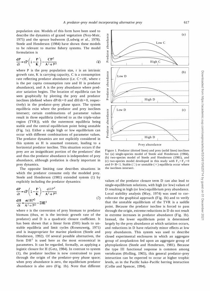
Prey is harvested, predator is not harvested. This situ-ation was analyzed by Collie and Spencer (1994) for thecase where B=1; allowing 0<B<1 does not change theessential features of the system. Harvesting of the preyspecies lowers the prey isocline in a manner shown inFigure 2a. Here, increasing F1 to high (or low) valuesresults in a single low (or high) prey equilibrium. Notethat as P]0 the prey isocline approaches £ so that

Prey abundance

Pre

dato

r ab

un

dan

ce

High D

Low D (c)P

reda

tor

abu

nda

nce

High F2

(b)

Pre

dato

r ab

un

dan

ce (a)

Low F2

Low F1

High F1

0

Figure 2. Predator (dotted lines) and prey (solid lines) isoclines;stable (,) or unstable (#) equilibria occur where the isoclinesintersect. (a) and (b) Effect of fishing mortality rates F1 and F2on the prey and predator isoclines, respectively. (c) Effect of thepredator closure term D when high levels of F2 result in anegative y-intercept of the predator isocline.


Dow


ic.oup.com/icesjm


ber 2021

changing F1 does not significantly affect this isocline atlow prey abundances, although it clearly affects theexistence of the lower equilibrium. Further, the rate offishing can be increased such that the hump in theisocline disappears.

Predator is harvested, prey is not harvested. Harvestingthe predator lowers the predator isocline but, in contrastto harvesting prey, the predator isocline is lowereduniformly over the entire range of prey abundances. Asan analogy to prey harvesting, high (or low) levels ofF2 result in high (or low) prey equilibria (Fig. 2b).Changes in F2 and D have similar effects on the predatorisocline, but the latter acts in a nonlinear manner due tothe quadratic closure term.At high levels of predator harvest, the predator

isocline has a negative y-intercept in the phase plane, asseen in Figure 2b. The value of the intercept is

H=

and negative values of the intercept will occur when thefishing mortality exceeds the population increase fromthe alternative prey (i.e. F2>ec(1"B)). This illustratesthe significance, in the model, of the alternative foodsource. Further, it can be shown that real-valued sol-utions for the x-intercept exist only for ec(1"B)<F2<ecand are independent of D. If a positive x-intercept exists,then as D]0 the y-intercept approaches "£ and thelocation of the lower equilibrium is constrained as thepredator isocline approaches a vertical line at low preyabundances (Fig. 2c). Thus, the dramatic increases inequilibrium predator abundance with decreased D arenot necessarily seen with predator harvesting.Predator fishing mortality can result in a single,

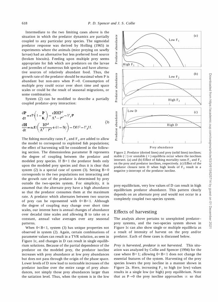
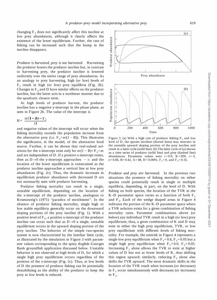
unstable equilibrium, depending on the location ofthe x-intercept of the predator isocline, analogous toRosenzweig’s (1971) ‘‘paradox of enrichment’’. In theabsence of predator fishing mortality, single high orlow stable equilibria generally occur on the downwardsloping portions of the prey isocline (Fig. 1). With apositive level of F2, a positive x-intercept of the predatorisocline can occur such that as D]0 a single, unstableequilibrium occurs in the upward sloping portion of theprey isocline. The behavior of the simple two-speciessystem is now characterized by the familiar limit cycle,as illustrated by the simulation in Figure 3 with param-eter values corresponding to the spiny dogfish–GeorgesBank groundfish application discussed below. Unstablebehavior is not observed at high levels of D, for which asingle high prey equilibrium occurs regardless of theposition of the x-intercept (Fig. 2c). Thus, at low levelsof D the presence of predator fishing can be potentiallydestabilizing as the ability of the predator to keep theprey at low levels is reduced.

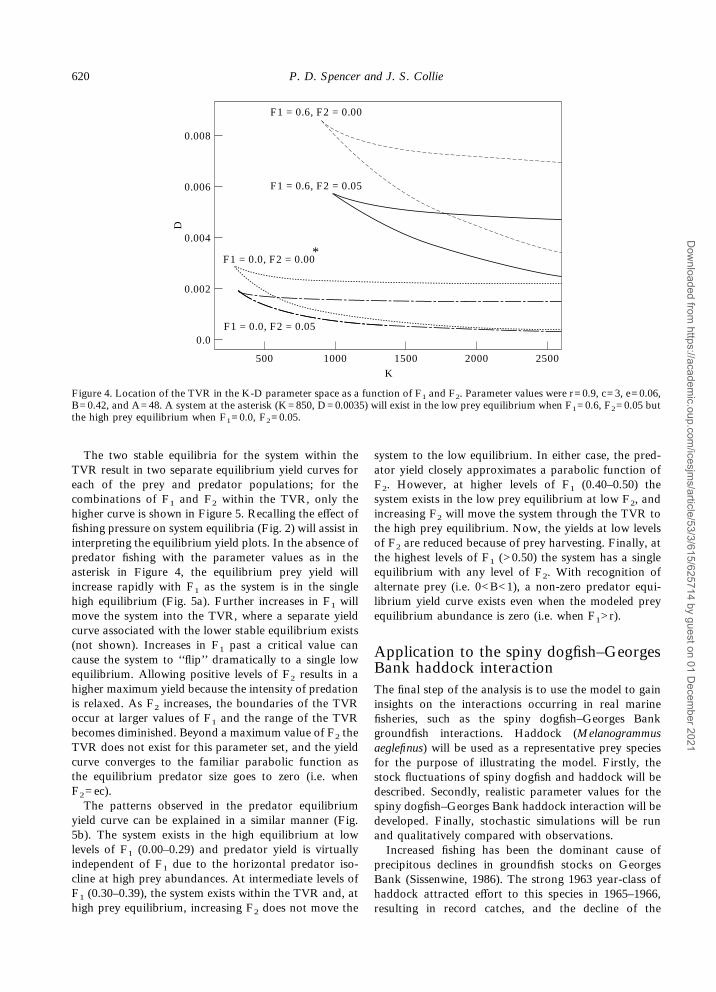
Predator and prey are harvested. In the previous twosituations the presence of fishing mortality on eitherspecies could potentially result in single or multipleequilibria, depending, in part, on the level of D. Withfishing on both species, the location of the TVR in theK–D parameter space varies as a function of both F1and F2. Each of the wedge shaped areas in Figure 4indicates the portion of the K–D parameter space wherea TVR solution exists for a given combination of fishingmortality rates. Parameter combinations above (orbelow) any individual TVR result in a high (or low) preyequilibrium; thus, a given combination of K and D mayexist in either the high prey equilibrium, TVR, or lowprey equilibrium with different levels of fishing mor-tality. For example, the asterisk in Figure 4 represents asingle low prey equilibrium when F1=0.6, F2=0.05 but asingle high prey equilibrium when F1=0.0, F2=0.05.Increasing F1 alone allows the TVR to exist at highervalues of D but not at lower levels of K, thus shiftingthis region upward; similarly, reducing F2 alone alsoshifts the TVR upward. The most dramatic shifts in thelocation of the TVR result when increases (or decreases)in F1 occur simultaneously with decreases (or increases)in F2.

Time

Pop

ula

tion

abu

nda

nce (b)

0 200 400 600 800 1000

Prey abundance

Pre

dato

r ab

un

dan

ce

(a)

Figure 3. (a) With a high rate of predator fishing F2 and lowlevel of D, the species isoclines (dotted lines) may intersect inthe unstable upward sloping portion of the prey isocline andresult in a limit cycle (solid line). (b) The limit cycle of (a) shownas a time series of predator (solid line) and prey (dashed line)abundances. Parameter values were r=0.9, K=850, c=3,e=0.06, B=0.42, A=48, D=0.0001, F1=0, and F2=0.16.


Dow


ic.oup.com/icesjm


ber 2021

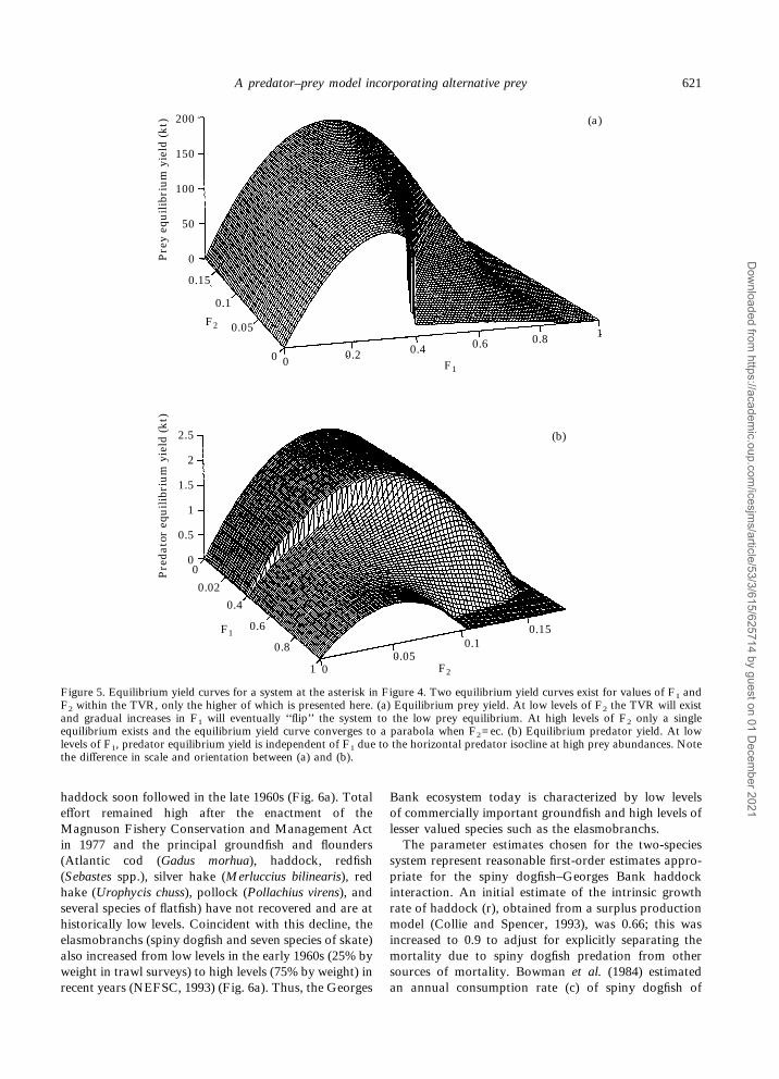
The two stable equilibria for the system within theTVR result in two separate equilibrium yield curves foreach of the prey and predator populations; for thecombinations of F1 and F2 within the TVR, only thehigher curve is shown in Figure 5. Recalling the effect offishing pressure on system equilibria (Fig. 2) will assist ininterpreting the equilibrium yield plots. In the absence ofpredator fishing with the parameter values as in theasterisk in Figure 4, the equilibrium prey yield willincrease rapidly with F1 as the system is in the singlehigh equilibrium (Fig. 5a). Further increases in F1 willmove the system into the TVR, where a separate yieldcurve associated with the lower stable equilibrium exists(not shown). Increases in F1 past a critical value cancause the system to ‘‘flip’’ dramatically to a single lowequilibrium. Allowing positive levels of F2 results in ahigher maximum yield because the intensity of predationis relaxed. As F2 increases, the boundaries of the TVRoccur at larger values of F1 and the range of the TVRbecomes diminished. Beyond a maximum value of F2 theTVR does not exist for this parameter set, and the yieldcurve converges to the familiar parabolic function asthe equilibrium predator size goes to zero (i.e. whenF2=ec).The patterns observed in the predator equilibrium

yield curve can be explained in a similar manner (Fig.5b). The system exists in the high equilibrium at lowlevels of F1 (0.00–0.29) and predator yield is virtuallyindependent of F1 due to the horizontal predator iso-cline at high prey abundances. At intermediate levels ofF1 (0.30–0.39), the system exists within the TVR and, athigh prey equilibrium, increasing F2 does not move the

system to the low equilibrium. In either case, the pred-ator yield closely approximates a parabolic function ofF2. However, at higher levels of F1 (0.40–0.50) thesystem exists in the low prey equilibrium at low F2, andincreasing F2 will move the system through the TVR tothe high prey equilibrium. Now, the yields at low levelsof F2 are reduced because of prey harvesting. Finally, atthe highest levels of F1 (>0.50) the system has a singleequilibrium with any level of F2. With recognition ofalternate prey (i.e. 0<B<1), a non-zero predator equi-librium yield curve exists even when the modeled preyequilibrium abundance is zero (i.e. when F1>r).

Application to the spiny dogfish–GeorgesBank haddock interactionThe final step of the analysis is to use the model to gaininsights on the interactions occurring in real marinefisheries, such as the spiny dogfish–Georges Bankgroundfish interactions. Haddock (Melanogrammusaeglefinus) will be used as a representative prey speciesfor the purpose of illustrating the model. Firstly, thestock fluctuations of spiny dogfish and haddock will bedescribed. Secondly, realistic parameter values for thespiny dogfish–Georges Bank haddock interaction will bedeveloped. Finally, stochastic simulations will be runand qualitatively compared with observations.Increased fishing has been the dominant cause of

precipitous declines in groundfish stocks on GeorgesBank (Sissenwine, 1986). The strong 1963 year-class ofhaddock attracted effort to this species in 1965–1966,resulting in record catches, and the decline of the

2500

0.008

0.0

K

D0.006

0.004

0.002

500 1500 2000

F1 = 0.0, F2 = 0.05

F1 = 0.0, F2 = 0.00*

F1 = 0.6, F2 = 0.05

F1 = 0.6, F2 = 0.00

1000

Figure 4. Location of the TVR in the K-D parameter space as a function of F1 and F2. Parameter values were r=0.9, c=3, e=0.06,B=0.42, and A=48. A system at the asterisk (K=850, D=0.0035) will exist in the low prey equilibrium when F1=0.6, F2=0.05 butthe high prey equilibrium when F1=0.0, F2=0.05.


Dow


ic.oup.com/icesjm


ber 2021

haddock soon followed in the late 1960s (Fig. 6a). Totaleffort remained high after the enactment of theMagnuson Fishery Conservation and Management Actin 1977 and the principal groundfish and flounders(Atlantic cod (Gadus morhua), haddock, redfish(Sebastes spp.), silver hake (Merluccius bilinearis), redhake (Urophycis chuss), pollock (Pollachius virens), andseveral species of flatfish) have not recovered and are athistorically low levels. Coincident with this decline, theelasmobranchs (spiny dogfish and seven species of skate)also increased from low levels in the early 1960s (25% byweight in trawl surveys) to high levels (75% by weight) inrecent years (NEFSC, 1993) (Fig. 6a). Thus, the Georges

Bank ecosystem today is characterized by low levelsof commercially important groundfish and high levels oflesser valued species such as the elasmobranchs.The parameter estimates chosen for the two-species

system represent reasonable first-order estimates appro-priate for the spiny dogfish–Georges Bank haddockinteraction. An initial estimate of the intrinsic growthrate of haddock (r), obtained from a surplus productionmodel (Collie and Spencer, 1993), was 0.66; this wasincreased to 0.9 to adjust for explicitly separating themortality due to spiny dogfish predation from othersources of mortality. Bowman et al. (1984) estimatedan annual consumption rate (c) of spiny dogfish of

0

F1

Pre

dato

r eq

uil

ibri

um

yie

ld (

kt)

2

2.5

1.5

1

0.5

0

0.02

0.4

0.6

0.8

1 00.05

0.10.15

F2

(b)

F2

Pre

y eq

uil

ibri

um

yie

ld (

kt) 200

150

100

50

0

0.15

0.1

0.05 1

0.2 0.4 0.6 0.8

F1

(a)

00

Figure 5. Equilibrium yield curves for a system at the asterisk in Figure 4. Two equilibrium yield curves exist for values of F1 andF2 within the TVR, only the higher of which is presented here. (a) Equilibrium prey yield. At low levels of F2 the TVR will existand gradual increases in F1 will eventually ‘‘flip’’ the system to the low prey equilibrium. At high levels of F2 only a singleequilibrium exists and the equilibrium yield curve converges to a parabola when F2=ec. (b) Equilibrium predator yield. At lowlevels of F1, predator equilibrium yield is independent of F1 due to the horizontal predator isocline at high prey abundances. Notethe difference in scale and orientation between (a) and (b).


Dow


ic.oup.com/icesjm


ber 2021

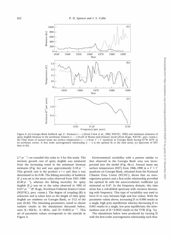
2.7 yr"1; we rounded this value to 3 for this study. Theintrinsic growth rate of spiny dogfish was estimatedfrom the increasing trend in the minimum biomassestimates (Fig. 6a) and was approximately 0.18 yr"1.This growth rate is the product e#c and thus e wasdetermined to be 0.06. The fishing mortality of haddock(F1) was set to the mean value observed from 1931–1990(0.40 yr"1), whereas the fishing mortality for spinydogfish (F2) was set to the value observed in 1992 of0.017 yr"1 (P. Rago, Northeast Fisheries Science Center(NEFSC), pers. comm.). The degree of coupling (B) isunknown and is taken here as the length of time spinydogfish are residents on Georges Bank, or 5/12 of theyear (0.42). The remaining parameters, tuned to obtainrealistic results in the simulations discussed below,were K=850 kt, A=48 kt, and D=0.0035 yr"1. Thisset of parameter values corresponds to the asterisk inFigure 4.

Environmental variability with a pattern similar tothat observed in the Georges Bank area was incor-porated into the model (Fig. 6b,c). Annual mean seasurface temperature (SST) from 1946–1990 in a 1)#1)quadrant on Georges Bank, obtained from the NationalClimatic Data Center (NCDC), shows that an auto-regressive pattern and a first-order relationship providedthe optimal fit with the autocorrelation coefficient (ñ)estimated as 0.47. In the frequency domain, this timeseries has a red-shifted spectrum with variance decreas-ing with frequency. This type of variability was used toforce D to vary between high and low values. With theparameter values above, increasing D to 0.006 results ina single, high prey equilibrium whereas decreasing D to0.001 results in a single, low prey equilibrium; the inter-mediate case of D=0.0035 results in the TVR (Fig. 7a).The simulations below were produced by varying D

with the first-order autoregressive relationship such that:

1.0

0.05Frequency (per year)

Var

ian

ce (

C2 p

er y

ear)

0.10

0.5

(c)

0.50

12

1950Year

Tem

pera

ture

(C

)

19609

(b)

1990

1000

1930Year

Bio

mas

s (k

t)

19700

(a)

1990

10

11

13

19801970

200

400

1940 1950 1960

800

600

1980

Figure 6. (a) Georges Bank haddock age 2+ biomass (——) (from Clark et al., 1982; NEFSC, 1992) and minimum estimates ofspiny dogfish biomass in the northwest Atlantic (– – –) (Gulf of Maine–mid-Atlantic stock) (from Rago, NEFSC, pers. comm.).(b) Time series of annual mean sea surface temperature (——) from 1)#1) quadrant in Georges Bank having 67)W 42)N asits northeast corner. A first order autoregressive relationship (– – –) is the optimal fit to the time series. (c) Spectrum of SSTdata in (b).


Dow


ic.oup.com/icesjm


ber 2021

Dt=ñDt"1+(1"ñ)D0+ìåt (7)

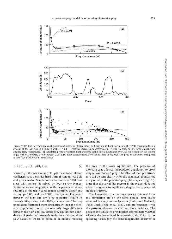
where D0 is the mean value of D, ñ is the autocorrelationcoefficient, å is a standardized normal random variableand ì is a scalar. Simulations were run over 1000 timesteps with system (3) solved by fourth-order Runge-Kutta numerical integration. With the parameter valuesresulting in the triple-value region identified above andsetting ñ=0.80, and ì=0.0011, the system fluctuatedbetween the high and low prey equilibria; Figure 7bshows a 300-yr slice of the 1000-yr simulation. The preypopulation fluctuated more dramatically than the pred-ator population due to the relatively large differencebetween the high and low stable prey equilibrium abun-dances. A period of favorable environmental conditions(low values of D) led to predator outbreaks, reducing

the prey to the lower equilibrium. The presence ofalternate prey allowed the predator population to growdespite low modeled prey. The effect of multiple attrac-tors can be seen clearly when the simulated abundancesare plotted in the predator–prey phase space (Fig. 7c).Note that the variability present in the system does notallow the system to equilibrate despite the presence ofstable attractors.The fluctuations for the prey species obtained from

this simulation are on the same decadal time scalesobserved in many marine fisheries (Caddy and Gulland,1983; Lluch-Belda et al., 1989), and are consistent withthe patterns observed in Georges Bank haddock. Thepeak of the simulated prey reaches approximately 360 ktwhereas the lower level is approximately 50 kt, corre-sponding to roughly the same magnitudes observed in

Figure 7. (a) The intermediate configuration of predator (dotted lines) and prey (solid line) isoclines in the TVR corresponds to asystem at the asterisk in Figure 4 with F1=0.4, F2=0.017; increases or decreases in D lead to high or low prey equilibriumabundances, respectively. (b) Simulated predator (dotted line) and prey (solid line) abundances over 300 time steps for the systemin (a) with D0=0.0035, ñ=0.8, and ì=0.0011. (c) Time series of simulated abundances in the predator–prey phase space; each pointis one year of the 300-yr simulation.


Dow


ic.oup.com/icesjm


ber 2021

the haddock stock. The pattern of predator abundance,increasing despite the modeled prey species being low,is consistent with the observed haddock–spiny dogfishpatterns (Fig. 6a).The simulated abundance of the prey population

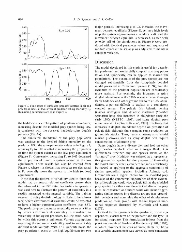
was sensitive to the level of fishing mortality on thepredator. With the same parameter values as in Figure 7,reducing F2 to 0.00 resulted in increasing the proportionof time the system existed at the low prey equilibrium(Figure 8). Conversely, increasing F2 to 0.05 decreasedthe proportion of time the system existed at the lowequilibrium. These results can also be inferred fromFigure 4, where it is shown that increases (or decreases)in F2 generally move the system to the high (or low)equilibrium.Note that the pattern of variability used to force the

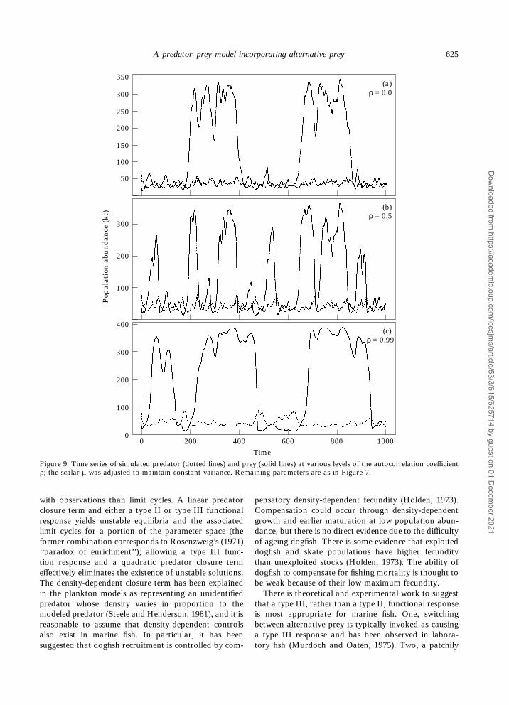
model had an autocorrelation coefficient greater thanthat observed in the SST data. Sea surface temperaturewas used here to illustrate the pattern of variability in areadily measured environmental variable. The habitatrelevant to spiny dogfish biology is likely to be subsur-face, where environmental variables would be expectedto have a higher autocorrelation coefficient than SST.The predator–prey dynamics essentially serve as a filterby which environmental variability is translated tovariability in biological processes, but the exact natureby which this occurs is unknown. Various assumptionsregarding the nature of variability lead to remarkablydifferent model outputs. With ñ=0, or white noise, theprey population exists at the high equilibrium for two

major periods; increasing ñ to 0.5 increases the move-ment between equilibria (Figure 9). At very high levelsof ñ the system approximates a random walk and themovement between equilibria is decreased, as seen withñ=0.99. All of the simulations in Figure 9 were pro-duced with identical parameter values and sequence ofrandom errors å; the scalar ì was adjusted to maintainconstant variance.

DiscussionThe model developed in this study is useful for describ-ing predators that are partially coupled to a prey popu-lation and, specifically, can be applied to marine fishpopulations. The dynamics of the prey species are notchanged substantially from the completely coupledmodel presented in Collie and Spencer (1994), but thedynamics of the predator population are considerablymore realistic. For example, the increases in spinydogfish abundance in the 1980s occurred when GeorgesBank haddock and other groundfish were at low abun-dances, a pattern difficult to explain in a completelycoupled system. The pelagic fish Atlantic herring(Clupea harengus) and Atlantic mackerel (Scomberscombrus) have also increased in abundance since theearly 1980s (NEFSC, 1993), and spiny dogfish preyupon these stocks (Overholtz et al., 1991). It is likely thatincreases in dogfish abundance depend on predation ofpelagic fish, although there remains some predation ongroundfish stocks. Thus, realistic attempts to modelmarine piscivores such as spiny dogfish will requireconsideration of alternate prey.Spiny dogfish have a diverse diet and feed on other

prey besides haddock when on Georges Bank; it isquestionable whether any one species serves as the‘‘primary’’ prey. Haddock was selected as a representa-tive groundfish species for the purpose of illustratingthe model, but the results seen here can most realisticallybe viewed as applying to the aggregate community ofsimilar groundfish species, including Atlantic cod.Groundfish are a logical choice for the modeled preybecause of the commercial importance of their dynam-ics, although one could view pelagic fish as the modeledprey species. In either case, the effect of alternative preymust be considered and future work will include aggre-gating similar species into discrete groups (e.g. ground-fish, pelagics) and examining the effect of simultaneouspredation on these groups with the multispecies func-tional responses discussed by Murdoch and Oaten(1975).Critical to the dynamics is the quadratic, or density-

dependent, closure term of the predator and the type IIIfunctional response. This formulation follows from theplankton models of Steele and Henderson (1981, 1992),in which movement between alternate stable equilibriain a variable environment was viewed as more consistent

Figure 8. Time series of simulated predator (dotted lines) andprey (solid lines) at two levels of predator fishing mortality F2.Remaining parameters are as in Figure 7.


Dow


ic.oup.com/icesjm


ber 2021

with observations than limit cycles. A linear predatorclosure term and either a type II or type III functionalresponse yields unstable equilibria and the associatedlimit cycles for a portion of the parameter space (theformer combination corresponds to Rosenzweig’s (1971)‘‘paradox of enrichment’’); allowing a type III func-tion response and a quadratic predator closure termeffectively eliminates the existence of unstable solutions.The density-dependent closure term has been explainedin the plankton models as representing an unidentifiedpredator whose density varies in proportion to themodeled predator (Steele and Henderson, 1981), and it isreasonable to assume that density-dependent controlsalso exist in marine fish. In particular, it has beensuggested that dogfish recruitment is controlled by com-

pensatory density-dependent fecundity (Holden, 1973).Compensation could occur through density-dependentgrowth and earlier maturation at low population abun-dance, but there is no direct evidence due to the difficultyof ageing dogfish. There is some evidence that exploiteddogfish and skate populations have higher fecunditythan unexploited stocks (Holden, 1973). The ability ofdogfish to compensate for fishing mortality is thought tobe weak because of their low maximum fecundity.There is theoretical and experimental work to suggest

that a type III, rather than a type II, functional responseis most appropriate for marine fish. One, switchingbetween alternative prey is typically invoked as causinga type III response and has been observed in labora-tory fish (Murdoch and Oaten, 1975). Two, a patchily

400

800Time

Pop

ula

tion

abu

nda

nce

(kt

)

200

(c)

6004000

100

0

300

ρ = 0.99

200 1000

200

(b)

100

300ρ = 0.5

200

(a)

100

300 ρ = 0.0

50

150

250

350

Figure 9. Time series of simulated predator (dotted lines) and prey (solid lines) at various levels of the autocorrelation coefficientñ; the scalar ì was adjusted to maintain constant variance. Remaining parameters are as in Figure 7.


Dow


ic.oup.com/icesjm


ber 2021

distributed prey combined with aggregation of predatorscan produce a type III response (Murdoch and Oaten,1975), and patchiness is a characteristic feature ofmarine systems. Finally, should a predator have a de-celerating type II response, it may involve a thresholdbelow which feeding does not occur; if this threshold isnormally distributed among individual predators a typeIII form will result for the population (Peterman, 1977).Unfortunately, empirical field data for marine fishpopulations are usually inadequate to confirm a specificfunctional response.Ecological systems can be classified with respect to the

causal mechanisms leading to variations in abundance,including stochasticity and overcompensatory bioticinteractions (DeAngelis and Waterhouse, 1987). In themodel presented here, exogenous forcing constantlymoves the system around and between two stable attrac-tors. Exogenous forcing alone can produce a remarkablearray of complex patterns; each of the simulations inFigure 9 was produced from the same simple model withidentical parameters values, and only the level of auto-correlation in the variability was changed. Allowingfishing mortality to vary could also result in the endog-enous dynamics demonstrated in this study. The limitcycle in Figure 3 could not occur in this model withoutpredator fishing, which essentially lowers the effectivegrowth rate of the predator and limits its ability tocontrol the prey. Although cyclic patterns in abundanceare suggested for some species, such as the CaliforniaDungeness crab, to our knowledge a pattern ofpredator–prey cycles has not been observed in marinefisheries. The relative importance of endogenous andexogenous mechanisms has been viewed differentlyamong ecologists; theoretical and terrestrial ecologistshave concentrated on the former (Turchin and Taylor,1992; Abrams and Roth, 1994), whereas the latter hasbeen discussed among marine ecologists (Steele, 1985).Our emphasis here on exogenous forcing is in recog-nition of the importance of variability in marine eco-systems, and the range of endogenous behavior is limitedby the two-dimensional differential equation format.More complex nonlinear models that explicitly considerthree (or more) species may reveal substantially morecomplex endogenous dynamics.The examination of the model with stochastic changes

in the density-dependent term, D, is consistent withthe earlier marine plankton models of Steele andHenderson, 1981, 1992), but in practice one wouldexpect environmental variability to affect several pro-cesses. Varying the intrinsic rate of growth, r, theconsumption rate, c, or the degree of coupling, B, leadsto similar flips between high and low prey abundancesbut not the dramatic increases in predator equilibriumabundances obtained by varying D. That variations in Dshould have this effect is easily seen; D is analogous tothe carrying capacity K in the traditional logistic model.

Environmental variability can affect population growthrates directly via density-independent rate processes(Beddington and May, 1977) or via density-dependentprocesses and equilibrium abundances (Roughgarden,1975; Shepherd and Horwood, 1979). The latter case isconsistent with variability at long time scales (Pimm,1984) and is used here. The highly simplified nature ofthe model and uncertainty of marine ecosystems doesnot allow specific consideration of how variability affectspopulations. Several mechanisms may be important inthe north-west Atlantic, including fish distributions.Spiny dogfish and their pelagic prey, Atlantic mackerel,are generally distributed at more northern latitudesduring warm years (Mountain and Murawski, 1992),and the dramatic increases in spiny dogfish and mackerelabundances in the 1980s occurred when water tempera-tures, on average, were higher than in the late 1960s(Holzwarth and Mountain, 1992).The model presented here can be used to address the

problem of finding the optimal combination of fishingmortality rates for the two species. A unique feature ofthis model is that nonlinear predation rates can causemultiple stable equilibria, differing from models withlinear predation rates (May et al., 1979). Increasedharvesting of a predator species generally results inincreased prey yield, but the presence of alternate stableequilibria makes these increases non-uniform. The pres-ence of fishing increases the potential causes for shiftsbetween equilibria relative to the earlier planktonmodels, as a shift to the low prey equilibrium can now becaused by either increased fishing on the prey, decreasedfishing on the predator, environmental variability, orsome combination of these factors. For example, therelatively high fishing mortality rates on spiny dogfishfrom 1971–1976 (P. Rago, NEFSC, pers. comm.) mayhave kept spiny dogfish biomass low, permitting apartial haddock recovery in the late 1970s (Fig. 6).The concept of multispecies management has particularrelevance for Georges Bank fisheries, as the task ofrebuilding the important groundfish stocks will requireconsideration of how exploitation of predators such asspiny dogfish affects recovery rates.The generality of the results above is limited because

of simplifications made with respect to age structure andtime delays. In particular, spiny dogfish generally do notconsume fish until they are approximately five years old(Overholtz et al., 1991). This may be stabilizing, asMaynard-Smith and Slatkin (1973) found in a theoreti-cal model with age-dependent predator hunting abilities.Predation on predominately young fish, such that preyage serves as a refuge, would also be expected to bestabilizing (May, 1974). Conversely, time delays in regu-latory processes are generally thought to be destabiliz-ing. Steele and Henderson (1981) found that introducinga time delay in the predator closure term DH2 increasedthe variability of predator–prey responses.


Dow


ic.oup.com/icesjm


ber 2021

In summary, an unsettling fact of any predator–preymodel is that it is impossible to incorporate all therelevant details into a simplified framework. Like system(2), system (3) is a grossly simplified depiction of reality,with the additional concept of alternative prey. From anecological viewpoint, it is desirable to have a moredetailed understanding of species interactions but, forfisheries management, it is necessary to have models thatcan be used with the data typically available for stockassessment. Obtaining unequivocal parameter estimatesis difficult even in the simplest single-species models, andadding model complexity further exacerbates the prob-lem. The lack of any precise fit of the model to the datashould not be surprising, as it is likely that severalvariables vary stochastically, resulting in the uniquerealizations seen in nature. With regard to spiny dogfishabundance, part of the lack of fit can be explainedsimply by defining population size; the observed datacorrespond to the entire spiny dogfish population in thenorthwest Atlantic, whereas the model pertains to onlythat portion of the stock that interacts with GeorgesBank haddock. Thus, the modeled spiny dogfishabundance (Fig. 7) is lower than the total estimateddogfish abundance (Fig. 6a). The model presented in thisstudy is a link between the completely coupled case ofCollie and Spencer (1994) and more complex three-species models. More detailed models will be pursued infuture research, while recognizing that optimal modelcomplexity is a compromise between desired realism andanalytical tractability.

Acknowledgements

We thank Glenn Strout and the staff at the FisheriesClimatology Investigation, NMFS, Narragansett,Rhode Island for providing the SST data. Paul Ragoprovided spiny dogfish biomass and fishing mortalityestimates. We are grateful to John Steele and HenrikGislason for their comments on an earlier draft. Thispublication is the result of research sponsored byRhode Island Sea Grant College Program with fundsfrom the National Oceanic and Atmospheric Ad-ministration, Office of Sea Grant, Department ofCommerce, under grant no. NA36RG0503 (project no.R/F-931).

ReferencesAndersen, K. P. and Ursin, E. 1977. A multispecies extension tothe Beverton and Holt theory, with accounts of phosphorouscirculation and primary production. Meddr. Danm. Fisk.-ogHavunders. N.S., 7: 319–435.

Abrams, P. A. and Roth, J. D. 1994. The effects of enrichmentof three-species food chains with nonlinear effects of preda-tion. Ecology, 75: 1118–1130.

Beddington, J. G. and May, R. M. 1977. Harvesting naturalpopulations in a randomly fluctuating environment. Science,197: 463–465.

Blinov, V. V. 1991. A robust approach to the analysis of feedingdata and an attempt to link multispecies virtual populationanalysis and Volterra predator–prey system analysis. ICESMarine Science Symposium, 193: 80–85.

Bowman, R. E., Eppi, R., and Grosslein, M. D. 1984. Diet andconsumption of spiny dogfish in the northwest Atlantic.ICES C.M. 1984/G: 27.

Caddy, J. F. and Gulland, J. A. 1983. Historical patterns of fishstocks. Marine Policy, 7: 267–278.

Clark, S. H., Overholtz, W. J., and Hennemuth, R. C. 1982.Review and assessment of the Georges Bank and Gulf ofMaine haddock fishery. Journal of Northwest AtlanticFishery Science, 3: 1–27.

Collie, J. S. and Spencer, P. D. 1993. Management strategies forfish populations subject to long-term environmental variabil-ity and depensatory predation. In Proceedings of the inter-national symposium on management strategies of exploitedfish populations, pp. 629–650. Ed. by G. H. Kruse, D. M.Eggers, R. J. Marasco, C. Pautzke, and T. J. Quinn. AlaskaSea Grant College Program Report No. 93–02. 825 pp.

Collie, J. S. and Spencer, P. D. 1994. Modeling predator–preydynamics in a fluctuating environment. Canadian Journal ofFisheries and Aquatic Sciences, 51: 2665–2672.

Conroy, M. J., Cohen, Y., James, F. C., Matsinos, Y. G., andMaurer, B. A. 1995. Parameter estimation, reliability, andmodel improvement for spatially explicit models of animalpopulations. Ecological Applications, 5: 17–19.

DeAngelis, D. L. and Waterhouse, J. C. 1987. Equilibrium andnonequilibrium concepts in ecological models. EcologicalMonographs, 57: 1–21.

Dunning, J. B. Jr, Stewart, D. J., Danielson, B. J., Noon, B. R.,Root, T. L., Lamberson, R. H., and Stevens, E. E. 1995.Spatially explicit population models: current forms andfuture uses. Ecological Applications, 5: 3–11.

Getz, W. M. 1984. Population dynamics: a per capita approach.Journal of Theoretical Biology, 108: 623–643.

Gislason, H. 1991. The influence of variations in recruitment onmultispecies yield predictions in the North Sea. ICES MarineScience Symposium, 193: 50–59.

Holden, M. J. 1973. Are long-term sustainable fisheries forelasmobranchs possible? Rapports et Procés-Verbaux desreunions du Conseil International pour l’Exploration de laMer, 164: 360–367.

Holling, C. S. 1965. The functional response of predators toprey density and its role in mimicry and population regu-lation. Memoirs of the Entomological Society of Canada, 45:1–60.

Holzwarth, T. and Mountain, D. 1992. Surface and bottomtemperature distributions from the Northeast FisheriesCenter spring and fall bottom trawl survey program, 1963–1987, with addendum for 1988–1990. NEFSC ReferenceDocument 90–03. 62 pp.

Kareiva, P. 1989. Renewing the dialogue between theory andexperiments in population ecology. In Perspectives in ecologi-cal theory, pp. 68–88. Ed. by J. Roughgarden, R. M. May,and S. A. Levin. Princeton University Press, Princeton, NJ.394 pp.

Lluch-Belda, D., Crawford, R. J. M., Kawasaki, T., MacCall,A. D., Parrish, R. H., Schwartzlose, R. A., and Smith, P. E.1989. World-wide fluctuations of sardine and anchovystocks: the regime problem. South African Journal of MarineScience, 8: 195–205.

Ludwig, D., Jones, D. D., and Holling, C. S. 1978. Qualitativeanalysis of insect outbreak systems: the spruce budworm andthe forest. Journal of Animal Ecology, 47: 315–332.

May, R. M. 1974. Stability and complexity in model eco-systems, 2nd ed. Princeton University Press, Princeton, NJ.265 pp.


Dow


ic.oup.com/icesjm


ber 2021

May, R. M. (Ed.) 1976. Theoretical ecology: principles andapplications. Blackwell Scientific Publications, Oxford,England. 317 pp.

May, R. M. 1977. Thresholds and breakpoints in ecosystemswith a multiplicity of stable states. Nature, 269: 471–477.

May, R. M., Beddington, J. R., Clark, C. W., Holt, S. J., andLaws, R. M. 1979. Management of multispecies fisheries.Science, 205: 267–277.

Maynard-Smith, J. and Slatkin, M. 1973. The stability ofpredator–prey systems. Ecology, 54: 384–391.

Mountain, D. G. and Murawski, S. A. 1992. Variation in thedistribution of fish stocks on the northeast continental shelfin relation to their environment, 1980–1989. ICES MarineScience Symposium, 195: 424–432.

Murdoch, W. W. and Oaten, A. 1975. Predation and popu-lation stability. Advances in Ecological Research, 9: 1–132.

NEFSC (Northeast Fisheries Science Center) 1992. Report ofthe thirteenth regional stock assessment workshop (13thSAW). NEFSC. Ref. Doc. 92-02. 183 pp.

NEFSC (Northeast Fisheries Science Center) 1993. Status ofthe fisheries resources off the northeastern United States for1993. NOAA Tech. Mem. NMFS-F/NEC-86. 140 pp.

Noy-Meir, I. 1975. Stability of grazing systems: an applicationof predator–prey graphs. Journal of Ecology, 63: 459–481.

Overholtz, W. J., Murawski, S. A., and Foster, K. L. 1991.Impact of predatory fish, marine mammals, and seabirds onthe pelagic fish ecosystem of the northeastern USA. ICESMarine Science Symposium, 193: 198–208.

Peterman, R. M. 1977. A simple mechanism that causes col-lapsing stability regions in expoited salmon populations.Journal of the Fisheries Research Board of Canada, 34:1130–1142.

Pimm, S. L. 1984. Food webs. Chapman and Hall, London.219 pp.

Rosenzweig, M. L. 1971. Paradox of enrichment: destabiliza-tion of exploitation ecosystems in ecological time. Science,171: 385–387.

Roughgarden, J. 1975. A simple model for population dy-namics in stochastic environments. American Naturalist,109: 713–736.

Shaefer, M. B. 1954. Some aspects of the dynamics of popu-lations important to the management of commercial marinefisheries. Bulletin of the Inter-American Tropical TunaCommission, 1: 27–56.

Shepherd, J. G. and Horwood, J. W. 1979. The sensitivity ofexploited populations to environmental ‘‘noise’’, and theimplications for management. Journal du Conseil Inter-national de la Mer, 38: 318–323.

Sissenwine, M. P. 1986. Perturbation of a predator-controlledcontinental shelf ecosystem. In Variability and managementof large marine ecosystems, pp. 55–85. Ed. by K. Sherman,K., and L. M. Alexander. Westview Press, Boulder, CO.319 pp.

Soutar, A. and Isaacs, J. D. 1974. Abundance of pelagic fishduring the 19th and 20th centuries as recorded in anaerobicsediment off the Californias. Fishery Bulletin, 72(2): 257–273.

Sparre, P. 1991. Introduction to multispecies virtual populationanalysis. ICES Marine Science Symposium, 193: 12–21.

Steele, J. H. 1985. A comparison of terrestrial and marineecological systems. Nature, 313: 355–358.

Steele, J. H. and Henderson, E. W. 1981. A simple planktonmodel. American Naturalist, 117: 676–691.

Steele, J. H. and Henderson, E. W. 1984. Modeling long-termfluctuations in fish stocks. Science, 224: 985–987.

Steele, J. H. and Henderson, E. W. 1992. The role of predationin plankton models. Journal of Plankton Research, 14:157–172.

Turchin, P. and Taylor, A. D. 1992. Complex dynamics inecological time series. Ecology, 73: 289–305.

Vance, P. R. 1978. Predation and resource partitioning in onepredator–two prey model communities. American Naturalist,112: 797–813.


Dow


ic.oup.com/icesjm


ber 2021

A simple predatorâ€“prey model of exploited marine fish populations

Documents