A simple inertial formulation of the shallow water ... et al... · A simple inertial formulation of the shallow water equations for efﬁcient ... a School of Geographical ... gradually

Journal of Hydrology 387 (2010) 33–45

Contents lists available at ScienceDirect

Journal of Hydrology

journal homepage: www.elsevier .com/ locate / jhydrol

A simple inertial formulation of the shallow water equations for efficienttwo-dimensional flood inundation modelling

Paul D. Bates a,*, Matthew S. Horritt b, Timothy J. Fewtrell a

a School of Geographical Sciences, University of Bristol, University Road, Bristol BS8 1SS, UKb Halcrow Ltd., Burderop Park, Swindon, Wiltshire SN4 0QD, UK

a r t i c l e i n f o

Article history:Received 27 May 2009Received in revised form 19 October 2009Accepted 22 March 2010

This manuscript was handled byK. Georgakakos, Editor-in-Chief, with theassistance of Ehab A. Meselhe, AssociateEditor

Keywords:Shallow water flowFlood propagationInundation modellingHydraulic modelling

0022-1694/$ - see front matter � 2010 Elsevier B.V. Adoi:10.1016/j.jhydrol.2010.03.027

* Corresponding author. Tel.: +44 117 928 9108; faE-mail address: [email protected] (P.D. Bate

s u m m a r y

This paper describes the development of a new set of equations derived from 1D shallow water theory foruse in 2D storage cell inundation models where flows in the x and y Cartesian directions are decoupled.The new equation set is designed to be solved explicitly at very low computational cost, and is here testedagainst a suite of four test cases of increasing complexity. In each case the predicted water depths com-pare favourably to analytical solutions or to simulation results from the diffusive storage cell code ofHunter et al. (2005). For the most complex test involving the fine spatial resolution simulation of flowin a topographically complex urban area the Root Mean Squared Difference between the new formulationand the model of Hunter et al. is �1 cm. However, unlike diffusive storage cell codes where the stabletime step scales with (1/Dx)2, the new equation set developed here represents shallow water wave prop-agation and so the stability is controlled by the Courant–Freidrichs–Lewy condition such that the stabletime step instead scales with 1/Dx. This allows use of a stable time step that is 1–3 orders of magnitudegreater for typical cell sizes than that possible with diffusive storage cell models and results in commen-surate reductions in model run times. For the tests reported in this paper the maximum speed upachieved over a diffusive storage cell model was 1120�, although the actual value seen will depend onmodel resolution and water surface gradient. Solutions using the new equation set are shown to begrid-independent for the conditions considered and to have an intuitively correct sensitivity to friction,however small instabilities and increased errors on predicted depth were noted when Manning’s n = 0.01.The new equations are likely to find widespread application in many types of flood inundation modellingand should provide a useful additional tool, alongside more established model formulations, for a varietyof flood risk management studies.

� 2010 Elsevier B.V. All rights reserved.

Introduction

Since first proposed by Zanobetti et al. (1970) methods to predictfloodplain inundation using storage cell approaches have becomejustifiably popular. Initially, such methods discretized floodplainsinto irregular polygonal units representing large (surface areas of100–101 km2) natural storage compartments and calculated thefluxes of water between these according to some uniform flow for-mulae such as the weir or Manning’s equations. For many suchmodels in-channel flows are calculated using some form of the1D Saint–Venant equations, and when bankfull flow is exceededwater is routed into and between the floodplain storage units. Mostcommercial 1D codes now include such a floodplain representation.More recently the availability of increased computing power anddetailed descriptions of floodplain topography available throughremote sensing (e.g. LiDAR data, Marks and Bates, 2000) has

ll rights reserved.

x: +44 117 928 7878.s).

allowed a move away from large, irregular storage units to the dis-cretization of the floodplain as a fine spatial resolution regular grid(cell areas of 10�2–10�3 km2). Here each cell within the grid is astorage area for which the mass balance is updated at each timestep according to the fluxes of water into and out of each cell. Sim-ilar to polygonal storage cell models, fluxes are calculated analyti-cally using uniform flow formulae but with the advantage ofhigher resolution predictions and removal of the need for the mod-eller to make explicit decisions about the location of storage com-partments and the linkages between these. Numerous suchmodels are now available (e.g. Estrela and Quintas, 1994; Bechteleret al., 1994; Bates and De Roo, 2000) and a similar blueprint hasincreasingly been adopted in commercial modelling packages (e.g.JFLOW by JBA Ltd., FlowRoute by Ambiental and the RMS Ltd., UKFlood Risk Model). Such models therefore solve a continuity equa-tion relating flow into a cell and its change in volume:

DhDt¼ DQ

DxDyð1Þ

http://dx.doi.org/10.1016/j.jhydrol.2010.03.027

mailto:[email protected]

http://www.sciencedirect.com/science/journal/00221694

http://www.elsevier.com/locate/jhydrol

34 P.D. Bates et al. / Journal of Hydrology 387 (2010) 33–45

and a flux equation for each direction where flow between cells iscalculated according to Manning’s law (only the x direction is givenhere):

Q i;jx ¼

h5=3flow

nhi�1;j � hi;j

Dx

!1=2

Dy ð2Þ

where hi,j is the water free surface height [L] at the node (i, j), Dxand Dy are the cell dimensions [L], t is the time [T], n is the Man-ning’s friction coefficient [L�1/3 T], and Qx and Qy describe the volu-metric flow rates between floodplain cells [L3 T�1]. Qy is definedanalogously to Eq. (2). The flow depth, hflow, represents the depththrough which water can flow between two cells, and is definedas the difference between the highest water free surface in thetwo cells and the highest bed elevation. These equations are solvedexplicitly using a finite difference discretization of the time deriva-tive term:

tþDthi;j � thi;j

Dt¼

tQ i�1;jx � tQ i;j

x þ tQ i;j�1y � tQ i;j

y

DxDyð3Þ

where th and tQ represent depth and volumetric flow rate at time trespectively, and Dt is the model time step which is held constantthroughout the simulation.

The advantage of the storage cell formulation is that fluxes arecalculated analytically so the computational costs per time step arepotentially much lower than in equivalent numerical solutions ofthe full shallow water equations. The method is also simple in con-cept and it is therefore relatively easy to develop and maintaincode that can perform the calculations. Such methods also inter-face readily with newly available remotely sensed terrain datawhich typically arrives in the form of a regular grid. For this reasonthe number of research and commercial codes based on these tech-niques has proliferated over the last decade (for a review see Hun-ter et al. (2007)). Whilst the method can only be applied togradually varied flows and does not include inertia or the abilityto capture supercritical effects, for many floodplain inundationproblems the representation is appropriate.

Such storage cell models were originally conceived for applica-tion at relatively coarse grid resolutions (25–100 m) and earlyapplications showed that at these scales there was a distinct com-putational advantage over full solutions of the 2D Saint–Venantequations (see for example Horritt and Bates, 2001, 2002). This al-lowed new applications of hydraulic models to be consideredincluding Monte Carlo uncertainty analysis (Aronica et al., 2002),inclusion of hydraulic models in ensemble forecasting chains (Pap-penberger et al., 2005) and model applications to domain scales or-ders of magnitude larger than anything previously attempted (e.g.Wilson et al., 2007). Despite these successes, a number of concernsbecame apparent. First, unless the constant time step used to solveEq. (3) was small, simulations with storage cell models quicklydeveloped ‘chequerboard’ type instabilities as all the water in aparticular cell drained into the adjacent ones in a single (large)time step (Cunge et al., 1980). At the next time step, this situationwould reverse and all the water would flow back. To solve thisproblem many modellers introduced some kind of ‘flow limiter’to prevent the solution over-shooting and too much water leavinga given cell in a single time step. The flow limiter sets the maxi-mum flow that can occur between cells and is typically a functionof flow depth, grid cell size and time step. In LISFLOOD-FP, forexample, the flow limiter used is:

Q i;jx ¼min Q i;j

x ;DxDyðhi;j � hi�1;jÞ

4Dt

!ð4Þ

This value is determined by considering the change in depth of acell, and ensuring it is not large enough to reverse the flow in or out

of the cell at the next time step. This limiter replaces fluxes calcu-lated using Manning’s equation with values dependent on modelparameters, and hence when the flow limiter is in use floodplainflows are sensitive to grid cell size and time step, and insensitiveto Manning’s n.

Flow limiters were rarely discussed in journal publications atthe time as their significance was not appreciated, but it was clearfrom the cell sizes and time steps used in these early applicationsthat for many cells at each time step a flow limiter was being in-voked. As a result flow-limited storage cell models often showedvery little sensitivity to floodplain friction and their results werestrongly dependent on the grid size and time step selected. Thereis a legitimate debate over the degree of sensitivity to floodplainfriction one should expect in an inundation model given that flood-plain velocities are usually very small, but the almost completelack of such sensitivity in certain applications of flow-limited stor-age cell models appeared to be more than could be explained inphysical terms.

A solution to this problem was provided by Hunter et al. (2005)based on adaptive time-stepping. This approach seeks to removethe need to invoke the flow limiter (Eq. (4)) by finding the opti-mum time step (large enough for computational efficiency, smallenough for stability) at each iteration. This optimum time step isobtained using an analysis of the governing equations and theiranalogy to a diffusion system which gives the following expressionfor Dt:

Dt ¼ Dx2

4min

2n

h5=3flow

@h@x

��1=2

;2n

h5=3flow

@h@y

��1=2

!ð5Þ

A scheme that uses this criterion can be implemented bysearching the domain for the minimum time step value and usingthis to update h in Eq. (3). The time step will thus be adaptive andchange during the course of a simulation, but is uniform in space ateach time step. Hunter et al. (2005) tested this new uncondition-ally stable time step formulation against analytical solutions forwave propagation over flat and planar slopes and showed a consid-erable improvement over the classical fixed time-step version ofthe model. Moreover, the adaptive scheme was shown to yield re-sults that were independent of grid size or choice of initial timestep and which showed an intuitively correct sensitivity to flood-plain friction over spatially-complex topography. Hunter et al.(2006) went on to test the new version of the LISFLOOD-FP modelagainst real world flood extent and wave travel time data for theupper River Severn in the UK for a model at 60 m spatial resolution.The adaptive time step model showed a better absolute perfor-mance than the classical fixed time-step version at this spatial res-olution, but at approximately six times the computational cost. Inparticular the adaptive model appeared able to simulate floodplainwetting and drying more realistically.

Despite this success, the results obtained by Hunter et al. (2006)identified a fundamental problem with Eq. (5), namely that theoptimum stable time step reduces quadratically with decreasinggrid size. For an explicit code this means that the computationalcost will increase as (1/Dx)4. For applications with grid sizes inthe range for which LISFLOOD-FP was originally designed (25–100 m, Bates and De Roo, 2000) this led to a 2–10� increase in sim-ulation times which could be offset through advances in processorspeed. Any residual cost increases could then be justified easily assimulations were more realistic. However, for the finer resolution(1–10 m) grids required for application of hydraulic models to ur-ban areas (Fewtrell et al., 2008) simulation costs increased by sev-eral orders of magnitude such that at these scales adaptive timestep storage cell codes actually proved slower than full 2D solu-tions of the shallow water equations. Hunter et al. (2008) foundduring benchmark testing of six 2D models applied at 2 m spatial

P.D. Bates et al. / Journal of Hydrology 387 (2010) 33–45 35

resolution to a 0.4 km2 area of Glasgow UK that numerical solu-tions of the full shallow water equations completed a 2 h real timesimulation in around 1 h (depending on code complexity and pro-cessor architecture), whilst the storage cell codes took approxi-mately an order of magnitude longer.

Although a less serious problem, the dependence of the timestep on the water surface slope in Eq. (5) also means that the timestep is reduced for areas with flat water surfaces, where intuitivelywe would expect the governing equations to be easier to solve. Inthe limit of a horizontal water surface, the time step is forced tozero, whereas the solution (zero flow in all directions) is trivial.In practice, the divergence of computation times in time-adaptivestorage cell models as the water comes to rest is avoided by apply-ing a linearization for small surface slopes (see Hunter et al., 2005).

Adaptive time step storage cell codes are therefore incompati-ble with the fine spatial resolution grids increasingly required forurban flood modelling. The only solution to date is to invoke a flowlimiter, but this leads to a poor representation of flow dynamics.Whilst for fine grids full 2D models give shorter simulation timesat current processor speeds, for practical applications they are stillonly able to treat small (<1 km2) areas at the required level of de-tail. It is clear that to allow wide area urban flood modelling at finespatial resolution a new hydraulic model formulation is required.Development and testing of such an approach is the fundamentalaim of this paper where we describe a set of flow equations foradaptive time step storage cell models which can overcome thequadratic dependency on grid size in Eq. (5) yet which can besolved analytically with approximately the same computationalcost as Eq. (2). The new scheme therefore retains all the computa-tional advantages of storage cell models over full 2D codes whoseequations require expensive numerical solution, yet with none ofthe previous disadvantages. Below we describe the derivation ofthe new set of equations from first principles, and then the newformulation is subject to a number of analytical and benchmarktests of increasing complexity. Finally, results are discussed andconclusions drawn.

Derivation of an inertial formulation of the shallow waterequations

The route to a new set of equations for fast inundation model-ling in two dimensions was identified in the urban model bench-marking study of Hunter et al. (2008). It was clear from thiscomparison that the lack of mass and inertia in Eq. (2) was thekey reason why storage cell models required the strict time stepcontrol implied by Eq. (5). In gradually varying shallow water flowsthe effect of inertia is to reduce fluxes between cells, yet in Eq. (5)flux is merely a function of gravity and friction. Eq. (5) thereforeoverestimates fluxes, particularly, as noted above, in areas of deepwater where there is only a small free surface gradient. Hunteret al. (2008) suggested that the solution was to modify explicitstorage cell codes to include inertial terms (or simple approxima-tions to these) that may allow the use of a larger stable time step,and hence quicker run times. In addition, inclusion of inertial ef-fects may also be important to represent the flow physics in partic-ular environmental settings.

Our starting point for derivation of such an equation is thereforethe momentum equation from the quasi-linearized one-dimen-sional Saint–Venant or Shallow Water equations:

@Q@t|{z}

acceleration

þ @

@xQ2

A

" #|fflfflfflfflffl{zfflfflfflfflffl}

advection

þ gA@ðhþ zÞ@x|fflfflfflfflfflfflffl{zfflfflfflfflfflfflffl}

water slope

þ gn2Q 2

R4=3A|fflfflffl{zfflfflffl}friction slope

¼ 0 ð6Þ

where Q [L3 T�1] is the discharge, A is the flow cross section area[L2], z is the bed elevation [L], R is the hydraulic radius [L], g is

the acceleration due to gravity [L T�2] and all other terms are de-fined as above. For many floodplains flows advection is relativelyunimportant (see Hunter et al. (2007) for a discussion of the magni-tude of terms in the shallow water equations) so we neglect thisterm, assume a rectangular channel and divide through by a con-stant flow width, w [L], to obtain an equation in terms of flow perunit width, q [L2 T�1]:

@q@tþ gh@ðhþ zÞ

@xþ gn2q2

R4=3h¼ 0 ð7Þ

For wide, shallow flows we can approximate the hydraulic ra-dius, R, with the flow depth, h. We can now discretize Eq. (7) withrespect to the time step, Dt, to give:

qtþDt � qt

Dt

� �þ ght@ðht þ zÞ

@xþ gn2q2

t

h7=3t

¼ 0 ð8Þ

And rearrange to give an explicit equation for q at time t + Dt:

qtþDt ¼ qt � ghtDt@ðht þ zÞ

@xþ n2q2

t

h10=3t

" #ð9Þ

This gives an equation for the unit flow at the next time step,qt+Dt, in terms of qt, ht and z and hence can be solved explicitly ata very similar cost to Eq. (2), as it contains only a single additionalterm. The advantage of this formulation is that since the accelera-tion term is now included, the water being modelled has somemass, and it is therefore less likely to generate the rapid reversalsin flow which lead to a chequerboard oscillation. Shallow waterwave propagation will also be represented, rather than the diffu-sive behaviour typical of previous storage cell models.

Eq. (9) can be improved further, since instabilities may still ariseat shallow depths when the friction term becomes large. Replacinga qt in the friction term by a qt+Dt leads to an equation linear in theunknown qt+Dt but which has some of the improved convergenceproperties of an implicit time stepping scheme:

qtþDt ¼ qt � ghtDt@ðht þ zÞ

@xþ n2qtqtþDt

h10=3t

" #ð10Þ

Eq. (10) can rearranged into an explicit form for calculation offlows at the new time step in the model:

qtþDt ¼qt � ghtDt @ðhtþzÞ

@x

1þ ghtDtn2qt=h10=3t

� � ð11Þ

The enhanced stability of Eq. (11) stems from the increase in thedenominator as the friction term increases, forcing the flow to zero,as would be expected for shallow depths. A similar approach isused in Liang et al. (2006) to improve the stability of a full 2D shal-low water model.

Unlike (2), Eq. (11) includes shallow water wave propagation sowhile stability is improved, it is still subject to the Courant–Freid-richs–Levy condition:

Cr ¼VDtDx

ð12Þ

where the non-dimensional Courant number, Cr, needs to be lessthan 1 for stability and V is a characteristic velocity [L T�1]. In thecase of a shallow water flow where advection is ignored this char-acteristic velocity is:ffiffiffiffiffiffi

ghp

ð13Þ

whereffiffiffiffiffiffigh

pis the celerity of a long wavelength, small amplitude

gravity wave. Eq. (12) gives a necessary but not sufficient condition


for model stability, and is used to estimate a suitable model timestep at t + Dt:

Dtmax ¼ aDxffiffiffiffiffiffiffight

p ð14Þ

where a is a coefficient in the range 0.2–0.7 used to produce a stablesimulation for most floodplain flow situations. The parameter a isincluded because Eq. (12) is not sufficient to ensure model stability,because the assumption of small amplitude in calculating the wavecelerity is not always valid, and because of the inclusion of frictionterms in the model. The stable time step is therefore often some-what less than that indicated by the Courant–Friedrichs–Lewy con-dition, and so the parameter a is introduced to reduce the time step.Despite these limitations in the application of the condition, Eq. (14)represents a useful approach to time step selection for a wide rangeof flow conditions, subject to an appropriate choice of a.

This time step is typically 1–3 orders of magnitude larger thanthe stable time step for the purely diffusive scheme of Eq. (5).Moreover, within this range, proportionally larger time step differ-ences become apparent as the grid size decreases, as for Eq. (14)time step scales with 1/Dx rather than (1/Dx)2. Hence, we expectthe new flux equation and adaptive time step constraint to be sig-nificantly more computationally efficient than previous storagecell models. The performance of this new set of equations andthe extent of this potential improvement is analysed in the follow-ing section.

Fig. 1. Predicted water surface elevation (z) at t = 3600 s for wave propagation overa horizontal beach simulated at 50 m spatial resolution and n = 0.03 using: (a) afixed time step (Dt = 1 s) flow limited diffusive model (Eqs. (2)–(4), light greydashed line); (b) an adaptive time step diffusive model (Eqs. (2), (3), and (5), midgrey dashed line); and (c) the new adaptive time step inertial model developed inthis paper (Eqs. (3), (11), and (14), dark grey dashed line). Each model is comparedto the analytical solution of Eq. (15) (solid black line). Summary numerical resultsfor these simulations are reported in Table 1.

Model testing and results

Eqs. (11) and (14) were implemented within the LISFLOOD-FPhydraulic model of Bates and De Roo (2000). This code has beendeveloped extensively since conception from a simple storage cellmodel written in the PC-RASTER language (Bates and De Roo,2000), to a flow limited code written in C++ (Horritt and Bates,2001) and finally to an adaptive time step code using Eq. (5) (Hun-ter et al., 2005, 2006). At each step previous variants were retainedin the code and can be readily switched on or off. Finally, the LIS-FLOOD-FP code has recently been placed within a version controlsystem, re-written in modular form (Fewtrell, 2009) and parallel-ized using Open-MP (Neal et al., 2009). Implementing and compar-ing new code variants is thus relatively straightforward givenprevious work on refining the code structure and bug fixing.

The new inertial formulation of LISFLOOD-FP was assessedagainst a structured sequence of numerical experiments that pro-vide a rigorous test of its numerical and computational perfor-mance. Three of these tests are taken from Hunter et al. (2005),and for the final test we simulate the urban flooding problem usedin the benchmarking studies of Hunter et al. (2008) and Fewtrellet al. (2008). Specifically these tests are:

Test 1: Non-breaking wave propagation over a horizontal planeand comparison to an analytical solution.Test 2: Non-breaking wave run-up on a planar beach and com-parison to an analytical solution.Test 3: Wetting and drying of a planar beach (i.e. a full tidalcycle).Test 4: Simulation of flood propagation through a complexstreet and building network at fine spatial resolution.

In each case the new inertial formulation is compared to theadaptive time step diffusive model (Eqs. (2) and (5)) of Hunteret al. (2005) in terms of root mean squared error (or difference),% volume error, minimum time step during the simulation and to-tal computational time. Tests 1–3 were run on a single 2.66 GHznode of a dual-core Intel Core2 Duo processor with 3 Gb of RAM,

whilst Test 4 was run on a single 2.8 GHz node of a quad-core IntelXeon Harpertown E5462 processor with 12 Mb of cache memory.The executables for both processors were built using the IntelC++ compiler. Test 4 has also been used by Hunter et al. (2008)to benchmark the performance of six 2D inundation models, byLamb et al. (2009) to evaluate an implementation of the JFLOWadaptive time step diffusive storage cell code designed to run onmassively parallel Graphics Processor Units (GPUs) and by Schu-bert et al. (2008) to test an unstructured finite element model forurban applications. These latter studies also report data on compu-tational efficiency which provides important information on thelikely comparative speed of models built with our new equationset.

Test 1: non-breaking wave propagation over a horizontal plane

Hunter et al. (2005) developed a one-dimensional analyticalsolution for inundation model testing where the full Saint–Venantequations can be simplified to yield an ordinary non-linear differ-ential equation. This can then be solved analytically to provide rig-orous validation solutions. The analytical solution presented belowis for the propagation of a non-breaking wave over a horizontalplane which allows us to test the ability of inundation models tosimulate wave movement correctly in the absence of a bed slopeterm (i.e. So = 0). In fact, this is not a true analytical solution tothe inertial equation solved by the model and thus we would notexpect the model results to fully converge to the analytical solutionalthough at fine grid resolutions it should be a close approxima-tion. The derivation of the analytical solution is given in Hunteret al. (2005) and is not repeated here, however the final equationfor the water depth, h, at any point in space x or at any time, t, is:

hx;t ¼73

C � n2u3ðx� utÞ� � 7=3

ð15Þ

where u is the component of depth-averaged velocity in the x direc-tion, C is a constant of integration, which can be fixed by referring tothe initial conditions of the problem (i.e. h at x = 0 and t = 0) and allother terms are defined as previously. Eq. (15) can now be used toprovide an analytical solution against which the model can betested with boundary conditions in the form of h(t) at x = 0, and ini-tial conditions in the form of h(x) at t = 0. Here this solution was

Table 1Summary of numerical and computational efficiency results from Tests 1, 2, 3 and 4.

Test case Model Root Mean Square Error (RMSE, in m) from analyticalsolution, or Root Mean Squared Difference (RMSD, inm), from diffusive model

Volume errorfrom analyticalsolution (%)

Minimum timestep duringsimulation (s)

Totalcomputationtime (min)

Speed upusinginertialversion

Test 1: horizontal beach,Dx = 50 m, n = 0.03

Diffusive 0.06 1.27 0.15 0.33Inertial 0.03 �1.25 7.25 0.02 17�

Test 2: planar beach,Dx = 50 m, n = 0.03

Diffusive 0.02 �0.17 0.02 1.22Inertial 0.11 �1.16 4.93 0.02 61�

Test 3: wetting and dryingof a planar beach,Dx = 50 m, n = 0.03

Diffusive – – 0.03 1.80Inertial See Fig. 7 – 5.59 0.03 60�

Test 4: Glasgow flooding,2 m resolution, spatiallyuniform friction

Diffusive 0.003 155.0Inertial 0.01 0.43 1.47 105�

Table 2Impact of grid resolution on RMSE and volume error for simulations of non-breakingwave propagation over a horizontal plane with n = 0.03.

Gridresolution(m)

Model Root MeanSquareError(RMSE, inm) fromanalyticalsolution

Volumeerrorfromanalyticalsolution(%)

Minimumtime stepduringsimulation(s)


5 Diffusive 0.006 �0.099 0.002 514.7Inertial 0.07 �2.37 0.73 2.33

10 Diffusive 0.013 0.071 0.006 32.02Inertial 0.065 �2.25 1.45 0.35



100 Diffusive 0.09 2.67 0.60 0.05Inertial 0.05 0.25 14.51 0.02

200 Diffusive 0.15 4.94 2.41 0.03Inertial 0.11 2.95 29.04 0.01


implemented using parameter values of u = 1 ms�1, Dx = 50 m andn = 0.03 m�1/3s for a simulation of duration 3600 s.

Fig. 1 shows the water surface elevations predicted by the diffu-sive and inertial models at the end of the simulation (i.e. att = 3600 s) compared to the analytical solution (solid black line) gi-ven by Eq. (15). For this case only, Fig. 1 also shows the water ele-vations predicted by a flow limited diffusive model with a fixedtime step of 1 s. The Root Mean Square Error (RMSE), volume error,minimum time step during the simulation and the total computa-tion time for each of these simulations are also summarised in Ta-ble 1. These results show that the new inertial formulation is ableto match the analytical solution well, with an RMSE half that of thediffusive solution (0.03 m compared to 0.06 m) and similar volumeerrors. By contrast, the flow limited diffusive model simulateswave propagation, wave front position and water depths poorlyand therefore is not considered here further. The minimum timestep achieved during the inertial model run is also �48� largerthan that for the diffusive model, and this translates to a 17� speedup in computational time. The gearing of minimum time step tocomputation time is due to the fact that: (a) for short simulationsthe fixed costs of running LISFLOOD-FP (data input and output,data consistency checks, etc.) actually become a relatively largeproportion of the total simulation time; and (b) timings for simu-lations which last only a few seconds may not necessarily be suffi-ciently precise. Hence the full speed up potential may not be seenfor this particular test case.

To test whether these results were sensitive to grid resolution,identical simulations were also run with the diffusive and inertialmodels at Dx = 5, 10, 25, 100 and 200 m. Predicted water eleva-

Fig. 2. Predicted water surface elevation (z) at t = 3600 s for wave propagation over a(denoted with dark to light grey lines respectively) and n = 0.03 using: (a) an adaptive timodel (dotted lines). Each model is compared to the analytical solution (solid black line

tions from these simulations at t = 3600 s are shown in Fig. 2 andsummarised in Table 2. The inertial model outperformed the diffu-sive model in terms of RMSE and volume error at Dx = 50, 100 and200 m, whereas the diffusive model was marginally better atDx = 5, 10 and 25 m. Errors are low for all resolution models apartfrom Dx = 200 m where the solution quality for both schemes isdominated by the effect of the coarse grid resolution which is

horizontal beach simulated at Dx = 5, 10, 25, 50, 100 and 200 m spatial resolutionme step diffusive model (dashed lines); and (b) the new adaptive time step inertial).


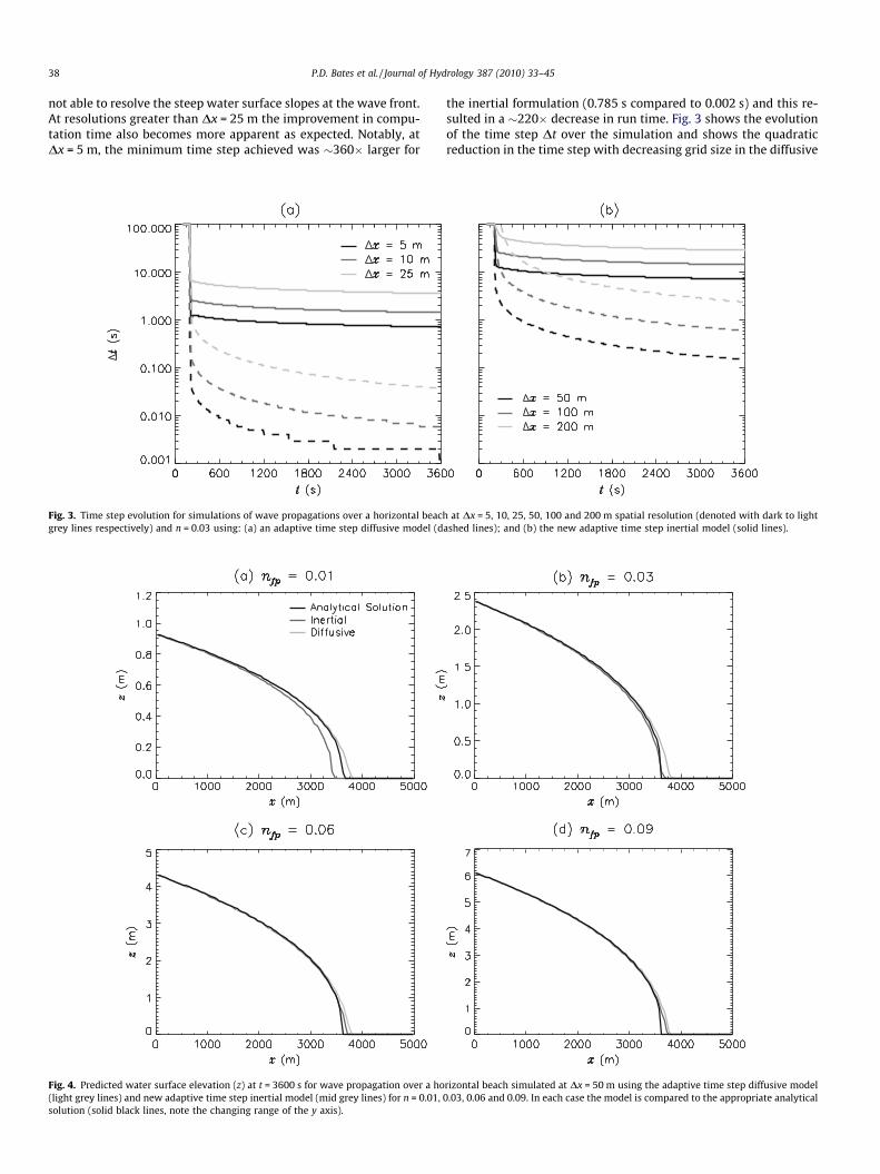
not able to resolve the steep water surface slopes at the wave front.At resolutions greater than Dx = 25 m the improvement in compu-tation time also becomes more apparent as expected. Notably, atDx = 5 m, the minimum time step achieved was �360� larger for

Fig. 3. Time step evolution for simulations of wave propagations over a horizontal beachgrey lines respectively) and n = 0.03 using: (a) an adaptive time step diffusive model (d

Fig. 4. Predicted water surface elevation (z) at t = 3600 s for wave propagation over a ho(light grey lines) and new adaptive time step inertial model (mid grey lines) for n = 0.01,solution (solid black lines, note the changing range of the y axis).

the inertial formulation (0.785 s compared to 0.002 s) and this re-sulted in a �220� decrease in run time. Fig. 3 shows the evolutionof the time step Dt over the simulation and shows the quadraticreduction in the time step with decreasing grid size in the diffusive

at Dx = 5, 10, 25, 50, 100 and 200 m spatial resolution (denoted with dark to lightashed lines); and (b) the new adaptive time step inertial model (solid lines).

rizontal beach simulated at Dx = 50 m using the adaptive time step diffusive model0.03, 0.06 and 0.09. In each case the model is compared to the appropriate analytical


models as a result of the Dx2 term in Eq. (5). Fig. 3 also shows thatwith the diffusive model the time step continues to decrease overthe simulation as depths increase and water surface slopes reduce.By contrast the reduction of time step with grid size in the inertialformulation is more linear, and after an initial period of evolutionstabilizes to a near uniform value as one would expect given thevelocity in the analytical solution is fixed at 1 ms�1.

Lastly, sensitivity to friction was assessed by running the diffu-sive and inertial models for n = 0.01, 0.03, 0.06 and 0.09 for a modelwith Dx = 50 m. Results from these simulations are presented inFig. 4 and Table 3 and show the inertial model outperforming thediffusive scheme at frictions above n = 0.03, but the performanceadvantage switching to the diffusive scheme for n = 0.01. Whythe behaviour should change for low values of n is unknown at thisstage. One possible explanation is that for low Manning’s numbersthere is insufficient dissipation inherently in the numerical schemeto dissipate the energy of the flow. Hence, at n = 0.01 the accelera-tion terms in the shallow water equations start to dominate andwe get wave-like behaviour, whereas inertial LISFLOOD-FP is de-signed for situations where there is a dominance of surface slopeand friction terms. Thus for model domains dominated by verylow surface friction a full shallow water model may give moreaccurate results. Even with this divergence from the analyticalsolution at n = 0.01, the RMSE for the inertial model is still only0.05 m and this is probably acceptable for many applications asthis is less than the vertical error in typically available terrain data(e.g. LiDAR). For both models RMSE errors increase with increasingfriction, to a maximum in these tests of 0.1 m for the inertialscheme and 0.14 m for the diffusive scheme at n = 0.09.

Test 2: non-breaking wave run-up on a planar beach

The second test case developed by Hunter et al. (2005) consistsof solving Eq. (15) for a planar beach (i.e. where So – 0). Here no di-rect analytical solution exists, but an accurate numerical solutionto Eq. (15) with uniform velocity can be obtained using a 4th orderRunge–Kutta scheme. Again this can be used to develop initial con-ditions, boundary conditions and a numerical solution againstwhich the model can be tested. This numerical solution was imple-mented using parameter values of u = 1 m s�1, Dx = 50 m,So = 10�3 mm�1 and n = 0.03 m�1/3s for a simulation of duration3600 s. Again the models are compared in terms of Root MeanSquare Error (RMSE), volume error, minimum time step duringthe simulation and the total computation time. These the resultsare summarised in Table 1. In this case the 50 m diffusive modelhas lower RMSE than the inertial model (0.02 m compared to0.11 m), but at a significantly greater computational cost. The min-imum time step for the diffusive model is �250� smaller than thatfor the inertial model and this translates into a simulation timethat is �61� longer. The greater speed up with the inertial modelhere is due to the fact that in this case the minimum water surface

Table 3Impact of friction on RMSE and volume error for simulations of non-breaking wavepropagation over a horizontal plane with Dx = 50 m.

Friction(Manning’sn)

Model Root Mean Square Error(RMSE, in m) from analyticalsolution

Volume error fromanalytical solution(%)

0.01 Diffusive 0.02 1.15Inertial 0.05 4.98

0.03 Diffusive 0.06 1.27Inertial 0.03 �1.25



slope is much smaller and hence Eq. (5) leads to smaller stable timesteps for the diffusive model. In fact the minimum time stepachieved over the simulation with the diffusive model is �20�smaller for a planar beach compared to the horizontal case at5 m resolution. This compares to a difference of only �1.5� forthe inertial model at the same scale. Despite its lower accuracy,the RMSE for the inertial model is still within the typical verticalerror of high resolution floodplain topographic surveys (e.g. thosederived using airborne laser altimetry) and likely to be less thanuncertainties induced by boundary condition errors. It should alsobe noted that the increase in depth for this test case is relativelyrapid compared to that which would be typical for most dynamicfloodplain inundation in lowland rivers. In reality in such situa-tions flow evolves much more gradually and hence Test 2 actuallyrepresents rather a stringent case. It may therefore be that formany practical applications the minor increase in errors in pre-dicted depth are acceptable given the large improvement in com-putational efficiency, and that these can, like any other modelstructural error, be compensated for during calibration.

In Fig. 5 we show the impact of changing model resolution onthe prediction of non-breaking wave run-up. This shows predictedwater surface elevations at t = 3600 s for the diffusive (dashedlines) and inertial models (dotted lines) at Dx = 5, 10, 25, 50, 100and 200 m. Here there is no impact of resolution on the model re-sults and the only differences are generated by the choice of modelformulation. All the diffusive model runs overlay the analyticalsolution, apart from where h ? 0 where the impact of grid sizecan be seen. All the inertial models also over plot, but lag thenumerical solution by a short distance. This result, in combinationwith the accuracy assessment in Table 4, suggests that the inertialmodels are in fact tending to a subtly different numerical solution,as noted above. The computation time for the inertial model atDx = 5 m is 1120� shorter than for the diffusive model as a resultof the large difference in stable time step (0.493 s compared to0.0001 s) which in turn is a consequence of the shallow water sur-face slope generated by this test case. Furthermore, Fig. 6 showsthat the under-prediction of wave front position is related to fric-tion and that the effect has largely disappeared when n = 0.06, atand above which both diffusive and inertial models performequally well. For the simulations at n = 0.01 there is also asuggestion of some minor instabilities with the inertial model.

Fig. 5. Predicted water surface elevation (z) at t = 3600 s for wave propagation up aplanar beach simulated at Dx = 5, 10, 25, 50, 100 and 200 m spatial resolution(denoted with dark to light grey lines respectively) and n = 0.03 using: (a) anadaptive time step diffusive model (dashed lines); and (b) the new adaptive timestep inertial model (dotted lines). Each model is compared to the numericalsolution (solid black line).

Table 4Impact of grid resolution on RMSE and volume error for simulations of non-breakingwave run-up on a planar beach with n = 0.03.

Gridresolution(m)

Model Root MeanSquareError(RMSE, inm) fromanalyticalsolution

Volumeerrorfromanalyticalsolution(%)

Minimumtime stepduringsimulation(s)









Test 3: wetting and drying of a planar beach

Tests 1 and 2 have tested the ability of the new model formula-tion to simulate wave propagation over flat and sloping flood-plains, however correct simulation of floodplain inundation overwhole events also requires the accurate representation of flowreversals and inundation front recession during floodplain drying.The ability of the model to do this can be evaluated by extendingTest 2 to represent wave run-up and drying through the imple-

Fig. 6. Predicted water surface elevation (z) at t = 3600 s for wave propagation up a plangrey lines) and new adaptive time step inertial model (mid grey lines) for n = 0.01, 0.03solution (solid black lines, note the changing range of the y axis).

mentation of a sinusoidal wave boundary condition at x = 0 (seefor example Leendertse and Gritton, 1971; Falconer and Chen,1991). In this case we use a wave of amplitude 4 m, period 4 h,and So = 10�3 m m�1 for a simulation of duration 7200 s. This givesboundary conditions comparable to those used in Test 2. As far asthe authors are aware, there is no analytical solution to this prob-lem so in this case we simply look at differences between the dif-fusive and inertial formulations. These are shown in Fig. 7 for asimulation using Dx = 50 m and n = 0.03. This shows smaller differ-ences between the inertial and diffusive formulations than for Test2. For example, the RMSD at the end of flow advance at 3600 s isonly 0.074 m, compared to 0.11 m for Test 2 at the same time.Overall, Fig. 7 shows wave front position during wetting and dryingsimulations to differ only marginally between the two formula-tions, and for wave shape to show noticeable differences only atthe start of flood wave recession (maximum RMSD of 0.137 m at4500 s). Compared to Test 2 the differences between the inertialand diffusive formulations at lower frictions are also less pro-nounced. This is shown in Fig. 8 where we compare the outputfrom dynamic wetting and drying simulations at t = 1800, 3600,5400 and 7200 s for n = 0.01, 0.03, 0.06 and 0.09 for both inertialand diffusive models. Maximum differences occur at t = 3600 sand 4500 s for n = 0.01 and n = 0.03, whilst at other times and forother frictions the results are only marginally different. This sug-gests that the differences between diffusive and inertial formula-tions shown in Figs. 5 and 6 may be a worst case scenario andthat differences may be less marked for more realistic cases.Fig. 8 also confirms the presence of small instabilities during theinitial phase of the simulation with the inertial model whenn = 0.01, however these die out as the simulation proceeds.

ar beach simulated at Dx = 50 m using the adaptive time step diffusive model (light, 0.06 and 0.09. In each case the model is compared to the appropriate numerical

Fig. 7. Predicted water surface elevation (z) during wetting and drying of a planar beach simulated using Dx = 50 m and n = 0.03 for: (a) an adaptive time step diffusive model(grey lines); and (b) the new adaptive time step inertial model (black lines).


In terms of computational cost, Test 3 should be relativelyexpensive for the diffusive model to solve as during flow reversaland the start of wave front recession the water surface profile be-comes near horizontal. Fig. 7 clearly shows this happening be-tween 4500 and 5400 s. Flow reversals are a necessary feature ofany dynamic flood simulation and cause the minimum time stepin a diffusive model to become very small because of the presenceof the free surface gradient terms in Eq. (5). Hence we would ex-pect greater computational savings with the inertial model for Test3 than for Tests 1 or 2. This is clearly shown in Table 1 where theinertial scheme results in a minimum time step �186� larger thanthat for the diffusive model and a total simulation time that is

Fig. 8. Predicted water surface elevation (z) during wetting and drying of a planar beachrespectively) for: (a) the new adaptive time step inertial model (top four panels) and (b

�60� shorter. Fig. 9 shows the time step evolution for the diffusiveand inertial simulations for Test 3 and highlights the fact that theminimum stable time step differs by 1–2 orders of magnitude overthe majority of the simulation. Moreover, as expected the time stepevolution for the inertial model is quasi-linear and after an initialperiod of evolution stabilizes to a near uniform value over thewhole simulation.

Test 4: fine spatial resolution simulation of urban inundation

Tests 1–3 have demonstrated the numerical and computationalperformance of the inertial formulation in a series of idealised

simulated using Dx = 50 m and n = 0.01, 0.03, 0.06 and 0.09 (black to light grey lines) an adaptive time step diffusive model (bottom four panels).

Fig. 9. Time step evolution during wetting and drying of a planar beach simulatedusing Dx = 50 m and n = 0.03 for: (a) an adaptive time step diffusive model (dashedline); and (b) the new adaptive time step inertial model (solid line).

Fig. 11. Event hydrograph simulated in Test 4. The vertical dashed lines at 30 and60 min represent instances for which model results are presented in later figures.


cases of increasing complexity. However, the critical test of themodel is whether it is able to simulate flood propagation over com-plex topography and reduce the long run times of storage cellcodes when applied at fine spatial resolution. To test this we usedthe new inertial formulation of LISFLOOD-FP to simulate the urbaninundation test case used in Hunter et al. (2008) and Fewtrell et al.(2008). This comprises a 1.0 � 0.4 km domain in the Greenfieldsarea of Glasgow, UK which has been observed to flood in responseto heavy rainfall in the small (�5 km2) upstream catchment. Forthis site digital elevation data at 1 m resolution were availablefrom an airborne laser altimetry survey that can be used to buildhigh resolution inundation models. This was supplemented byHunter et al. (2008) with Ordnance Survey (OS) Mastermap� digi-tal map data that defined building locations, the road network andland-use type as vector layers. The LiDAR data acquired for thisstudy had already been filtered to remove vegetation and buildingfeatures to leave a ‘bare earth’ digital elevation model (DEM) withhorizontal and vertical accuracies less than 50 cm and 15 cm RootMean Square Error (RMSE) respectively. For hydraulic modellingHunter et al. (2008) aggregated the ‘bare earth’ LiDAR data to2 m and reinserted buildings, kerbs and roads based on their loca-tions in the digital map layer. Fig. 10 shows: (a) the road and build-ing layout at this study site overlaid onto the surface height (z)from the benchmark DEM and (b) a high resolution aerial photoof the same area.

(a)

Fig. 10. The Greenfields study site (Test 4): (a) building and road topology derived fromDEM shown as a grey scale and (b) high resolution aerial photo of the study site. All mapnorth–south along the y axis. Dimensions are in m.

Flooding at this site is caused, at least in part, by a small (�1 mwide) stream that enters near the north-east corner of the domain(located at point XQ on Fig. 10a) and almost immediately enters aculvert that runs under the entire site. Flooding has been observedto occur here as a result of flow exceeding the capacity of the cul-vert and spilling into the street network. Once the capacity of theculvert is exceeded water flows along two main east–west orientedstreets before converging and ponding in low-lying areas in thesouthern part of the domain.

The flow event simulated is based on a real flood that occurredat this site on 30 July 2002. The inflow boundary condition con-sisted of the hydrograph shown in Fig. 11, which was imposed asa point source internal to the model domain at location XQ. Thishydrograph represents the water volume overflowing the culvertand lasts <60 min, but as in Hunter et al. (2008) simulations werecontinued for 120 min to allow water to come to rest and pond indepressions. All external boundaries for each model were closed asmass flux across the external boundary is negligible. Lastly, frictionwas represented as in Fewtrell et al. (2008) using a single compos-ite value of n = 0.035. This was selected based on the spatial distri-bution of land use within the domain as determined from the OSMastermap� data.

Simulations were run with these data using the adaptive timestep storage cell formulation of Hunter et al. (2005) and the newinertial formulation developed in this paper. Fig. 12 shows the pre-dicted water depths at the end of the simulation (120 min) for bothformulations and a map of the absolute differences in water depth(diffusive minus inertial) at this time. Overall flood extents differonly marginally and the Root Mean Squared Difference in water

(b)

Ordnance Survey Mastermap� data with the surface height (z) from the benchmarkplots are in Cartesian coordinates where east–west is oriented along the x axis and


depth is only 0.01 m (see Table 1). Maximum differences in waterdepth are ±0.1 m, but these are very localized and over the major-ity of the domain water depth differences are close to the RMSD.The largest difference occurs at x = 180, y = 250 where the flood ex-tent is slightly greater in the diffusive version and fills up a small(�0.1 m deep) depression not flooded by the inertial model. Otherareas of difference, such as the higher predicted depths in the iner-tial model at x = 700, y = 200 at the end of the simulation, may be aresult of the additional physics in this scheme obtained by includ-ing the acceleration terms from the full shallow water equations.The run time for this test is �105� shorter for the inertial model(1.47 min compared to 155 min for the diffusive model) which isin line with theoretical expectations. The total computation timefor the inertial model also compares favourably with the run timesreported for other classes of model applied at this test site. Theseinclude Hunter et al. (2008) who report run times of around60 min for various structured grid, full shallow water models,Schubert et al. (2008) who report a �18 min run time for a 2 m res-

Fig. 12. Predicted water depths for at the end of the simulation for Test 4 (120 min) usinthe new adaptive time step inertial model. Panel (c) shows the difference in predicted w

olution unstructured grid, full shallow water model and Lamb et al.(2009) who report a �9 min run time for a structured grid, adap-tive time step diffusive model (JFLOW) run on a massively parallelGraphics Processor Unit (GPU). Whilst these are not controlledtests conducted with identical processors and compilers (for exam-ple the processors used for the simulations reported by Hunteret al. are now relatively old), these results do suggest that thenew inertial formulation would be faster for this case than any pre-viously applied code. This is a significant advance on diffusive stor-age cell models which were shown by Hunter et al. (2008) to be anorder of magnitude slower than full shallow water models at thisresolution because of the quadratic dependency on grid size inEq. (5). Moreover, when one couples the speed up achieved herewith the 5–6� speed up in LISFLOOD-FP run times achieved byNeal et al. (2009) using Open-MP parallelization on an 8 coreprocessor, the potential for a �600� reduction in run times forthis test case (i.e. down to �0.25 min) becomes a realisticexpectation.

g a grid resolution of Dx = 2 m for: (a) an adaptive time step diffusive mode and (b)ater depths (diffusive minus inertial) between (a) and (b).


Discussion and conclusions

The results outlined in the preceding section show the newinertial formulation of the shallow water equations developed inthis paper to produce flow predictions that compare favourablywith analytical solutions for non-breaking wave propagation overhorizontal and planar beaches and to the results from an adaptivetime step diffusive storage cell code. Like the diffusive model, theinertial code is relatively insensitive to grid resolution and displaysan intuitively correct response to changing friction.

The inertial code performs slightly better than the diffusivecode for a horizontal beach and slightly worse for a planar beachwhen compared to the analytical solution. However for either codethe Root Mean Squared Error is always less than the typical verticalerror (�0.1 m) in high resolution terrain data (such as airborne la-ser altimetry or LiDAR) used for inundation modelling. Waterdepth errors are independent of grid scale but do vary with friction,with the inertial model tending to perform worse than the diffu-sive model when n = 0.01. Differences between the inertial and dif-fusive codes become less marked for more realistic cases involvingdynamic wetting and drying and for higher frictions, and for a realtest case involving the fine spatial resolution simulation of flow ina topographically complex urban area the Root Mean Squared Dif-ference is �1 cm. Whilst water depths predicted by the new for-mulation are similar to benchmark solutions, these results areachieved at a significantly reduced computational cost becausethe minimum stable time step scales with Dx, rather than with(1/Dx)2 as would be the case for a purely diffusive scheme. The ex-act speed up over a diffusive code will depend on grid resolutionand water surface gradients within the flow domain but from the-oretical considerations is likely to be 1–3 orders of magnitude. Themaximum speed up achieved for the tests reported here is 1120�and as a result the inertial code will most likely be faster thaneither diffusive or full shallow water models at any given spatialresolution. Moreover, as the explicit equation we here describe isrelatively easy to code it should be simple to parallelize usingOpen-MP techniques (e.g. Neal et al., 2009) or software tools suchas NVIDIA’s Kuda which allow models to run on massively parallelGPU cards (e.g. Lamb et al., 2009). This will pave the way to furthersubstantial reductions in run times and make possible a wholerange of new applications of hydraulic models. These could includewhole city risk analyses at the native spatial resolution of LiDARdata (i.e. 0.25–1 m), real time two-dimensional inundation fore-casting using ensemble data assimilation, multi-year simulationsof flows at continental scales (e.g. the Amazon River basin, Wilsonet al., 2007), and explorations of model uncertainty using MonteCarlo analyses with orders of magnitude more realisations thanhas hitherto been possible.

Care should be taken when using the new inertial formulationfor domains where large areas of low friction land use dominate(i.e. where n is equal to �0.01), as here predicted water depth er-rors increase and small instabilities can creep into the solution.The instability seen at low Manning’s n results from the hybrid nat-ure of the model, and shortcomings in the stability criteria applied.The Courant–Friedrichs–Lewy condition is more usually applied toadvective problems where upwinding is applied, and thus may notbe strictly applicable to the centred difference approach adoptedhere. Hunter et al. (2005) showed that without the inertia terms,stable time step is proportional to n (Eq. (5)), and hence will be dri-ven to zero if the friction is neglected. Friction is acting to stabilisethe scheme in this respect, with stability increased further by addi-tion of the inertia term as described in this paper. A rigorous anal-ysis of the stability of a non-linear model including both frictionand wave propagation behaviour will be complex, if not impossi-ble, but the analysis presented here is a pragmatic approach takinginto account the limiting behaviours understood by the Courant–

Friedrichs–Lewy condition and the approach of Hunter et al.(2005). This approach has been shown to be reasonable throughthe test cases presented in this paper, for models of typical naturalfloodplains. While the absence of a rigorous analysis of stability is adrawback compared to other numerical schemes, in some circum-stances this is outweighed by the advantages of simplicity, whichmake implementation on parallel and non-standard architecturesas discussed above far easier. However, for model domains charac-terised by very low surface friction a full shallow water model maygive more accurate results.

Future research should test the new inertial formulation for fur-ther test cases and seek to benchmark model performance (interms of both predictions and computational times) against a vari-ety of other model types in controlled experiments such as thosedescribed by Hunter et al. (2008). Further work should also be con-ducted to try to improve stability of the new equation set at lowfriction or examine the possibility of developing models capableof using different physical formulations in different parts of themodel domain depending on changing flow dynamics. A spatiallyvarying time step may also improve model efficiency, althoughprevious work on this for 1D models shows that the potentialspeed up is reduced significantly by other computational over-heads associated with changing the time step for different partsof the model (Wright et al., 2003). Despite this need for ongoing re-search, this paper has demonstrated the utility of the new inertialformulation against a series of stringent tests of increasing com-plexity. The new equations are therefore likely to find widespreadapplication in many types of flood inundation modelling andshould provide a useful additional tool, alongside more establishedmodel formulations, for a variety flood risk management studies.

Acknowledgements

Timothy Fewtrell’s work on this paper forms part of his Re-search Fellowship funded by the Willis Research Network (http://www.willisresearchnetwork.com). The University of Bristol Blue-Crystal high performance computer was used to undertake thesimulations reported in this paper.

References

Aronica, G., Bates, P.D., Horritt, M.S., 2002. Assessing the uncertainty in distributedmodel predictions using observed binary pattern information within GLUE.Hydrological Processes 16 (10), 2001–2016.

Bates, P.D., De Roo, A.P.J., 2000. A simple raster-based model for flood inundationsimulation. Journal of Hydrology 236 (1–2), 54–77.

Bechteler, W., Hartmann, S., Otto, A.J., 1994. Coupling of 2D and 1D models andintegration into Geographic Information Systems (GIS). In: White, W.R., Watts,J. (Eds.), 2nd International Conference on River Flood Hydraulics. John Wileyand Sons Ltd., Chichester, pp. 155–166.

Cunge, J.A., Holly, F.M., Verwey, A., 1980. Practical Aspects of Computational RiverHydraulics. Pitman Publishing, London. 420 pp.

Estrela, T., Quintas, L., 1994. Use of a GIS in the modelling of flows on floodplains. In:White, W.R., Watts, J. (Eds.), 2nd International Conference on River FloodHydraulics. John Wiley and Sons Ltd., Chichester, pp. 177–190.

Falconer, R.A., Chen, Y., 1991. An improved representation of flooding and dryingand wind stress effects in a 2-D tidal numerical model. Proceedings ofInstitution of Civil Engineers: Research and Theory 91 (12), 659–678.

Fewtrell, T.J., 2009. Development of simple numerical methods for improving two-dimensional hydraulic models of urban flooding. Unpublished Ph.D. Thesis,University of Bristol.

Fewtrell, T.J., Bates, P.D., Horritt, M., Hunter, N., 2008. Evaluating the effect of scalein flood inundation modelling in urban environments. Hydrological Processes22, 5107–5118.

Horritt, M.S., Bates, P.D., 2001. Predicting floodplain inundation: raster-basedmodelling versus the finite-element approach. Hydrological Processes 15 (5),825–842.

Horritt, M.S., Bates, P.D., 2002. Evaluation of 1-D and 2-D numerical models forpredicting river flood inundation. Journal of Hydrology 268 (1–4), 87–99.

Hunter, N.M., Horritt, M.S., Bates, P.D., Wilson, M.D., Werner, M.G.F., 2005. Anadaptive time step solution for raster-based storage cell modelling of floodplaininundation. Advances in Water Resources 28, 975–991.

http://www.willisresearchnetwork.com

http://www.willisresearchnetwork.com


Hunter, N.M., Bates, P.D., Horritt, M.S., Wilson, M.D., 2006. Improved simulation offlood flows using storage cell models. Proceedings of the Institution of CivilEngineers, Water Management 159 (1), 9–18.

Hunter, N.M., Bates, P.D., Horritt, M.S., Wilson, M.D., 2007. Simple spatially-distributed models for predicting flood inundation: a review. Geomorphology90, 208–225.

Hunter, N.M., Bates, P.D., Neelz, S., Pender, G., Villanueva, I., Wright, N.G., Liang, D.,Falconer, R.A., Lin, B., Waller, S., Crossley, A.J., Mason, D., 2008. Benchmarking2D hydraulic models for urban flood simulations. Proceedings of the Institutionof Civil Engineers, Water Management 161 (1), 13–30.

Lamb, R., Crossley, A., Waller, S., 2009. A fast 2D floodplain inundation model.Proceedings of the Institution of Civil Engineers, Water Management 162 (1), 1–9.

Leendertse, J.J., Gritton, E.C., 1971. A Water Quality Simulation Model for Well-mixed Estuaries and Coastal Seas, vol. 2. Computation Procedures. The RandCorporation, Santa Monica, Report R-708-NYC.

Liang, D., Falconer, R.A., Lin, B., 2006. Improved numerical modelling of estuarineflows. Proceedings of the Institution of Civil Engineers, Maritime Engineering159 (1), 25–35.

Marks, K., Bates, P.D., 2000. Integration of high-resolution topographic data withfloodplain flow models. Hydrological Processes 14, 2109–2122.

Neal, J.C., Fewtrell, T.J., Trigg, M.A., 2009. Parallelisation of storage cell floodmodels using OpenMP. Environmental Modelling and Software 24 (7),872–877.

Pappenberger, F., Beven, K.J., Hunter, N., Bates, P.D., Gouweleeuw, B., Thielen, J., DeRoo, A.P.J., 2005. Cascading model uncertainty from medium range weatherforecasts (10 days) through a rainfall–runoff model to flood inundationpredictions within the European Flood Forecasting System (EFFS). Hydrologyand Earth System Science 9 (4), 381–393.

Schubert, J.E., Sanders, B.F., Smith, M.J., Wright, N.G., 2008. Unstructured meshgeneration and landcover-based resistance for hydrodynamic modeling ofurban flooding. Advances in Water Resources 31 (12), 1603–1621.

Wilson, M.D., Bates, P.D., Alsdorf, D., Forsberg, B., Horritt, M., Melack, J., Frappart, F.,Famiglietti, J., 2007. Modeling large-scale inundation of Amazonian seasonallyflooded wetlands. Geophysical Research Letters 34 (Paper No. L15404).

Wright, N.G., Whitlow, C., Crossley, A., 2003. Local time stepping for modeling openchannel flows. American Society of Civil Engineers, Journal of HydraulicEngineering 129 (6), 455–462.

Zanobetti, D., Longeré, H., Preissmann, A., Cunge, J.A., 1970. Mekong deltamathematical model program construction. American Society of CivilEngineers, Journal of the Waterways and Harbors Division 96 (WW2),181–199.

A simple inertial formulation of the shallow water ... et al... · A simple inertial formulation of the shallow water equations for efﬁcient ... a School of Geographical ... gradually

Documents