A Short Course on Polar Coding Theory and Applications Prof. Erdal Arıkan Electrical-Electronics Engineering Department, Bilkent University, Ankara, Turkey Center for Wireless Communications, University of Oulu, 23-25 May 2016 Table of Contents L1: Information theory review L2: Gaussian channel L3: Algebraic coding L4: Probabilistic coding L5: Channel polarization L6: Polar coding L7: Origins of polar coding L8: Coding for bandlimited channels L9: Polar codes for selected applications L1: Information theory review L2: Gaussian channel L3: Algebraic coding L4: Probabilistic coding L5: Channel polarization L6: Polar coding L7: Origins of polar coding L8: Coding for bandlimited channels L9: Polar codes for selected applications L1: Information theory review 1/20 Lecture 1 – Information theory review ◮ Objective ◮ Establish notation ◮ Review the channel coding theorem ◮ Reference for this part: T. Cover and J. Thomas, Elements of Information Theory, 2nd ed., Wiley: 2006. L1: Information theory review 2/20

Welcome message from author
This document is posted to help you gain knowledge. Please leave a comment to let me know what you think about it! Share it to your friends and learn new things together.
Transcript

A Short Course on Polar Coding
Theory and Applications
Prof. Erdal Arıkan
Electrical-Electronics Engineering Department,Bilkent University, Ankara, Turkey
Center for Wireless Communications,University of Oulu, 23-25 May 2016
Table of Contents
L1: Information theory review
L2: Gaussian channel
L3: Algebraic coding
L4: Probabilistic coding
L5: Channel polarization
L6: Polar coding
L7: Origins of polar coding
L8: Coding for bandlimited channels
L9: Polar codes for selected applications
L1: Information theory review
L2: Gaussian channel
L3: Algebraic coding
L4: Probabilistic coding
L5: Channel polarization
L6: Polar coding
L7: Origins of polar coding
L8: Coding for bandlimited channels
L9: Polar codes for selected applications
L1: Information theory review 1/20
Lecture 1 – Information theory review
◮ Objective
◮ Establish notation
◮ Review the channel coding theorem
◮ Reference for this part: T. Cover and J. Thomas, Elements ofInformation Theory, 2nd ed., Wiley: 2006.
L1: Information theory review 2/20
Notation and conventions - I
◮ Upper case letters X ,U,Y , . . . denote random variables
◮ Lower case letters x , u, y , . . . denote realization values
◮ Script letters X ,Y, · · · denote alphabets
◮ XN = (X1, . . . ,XN) denotes a vector of random variables
◮ X ji = (Xi , . . . ,Xj) denotes a sub-vector of XN
◮ Similar notation applies to realizations: xN and x ji
L1: Information theory review Notation 3/20
Notation and conventions - II
◮ PX (x) denotes the probability mass function (PMF) on adiscrete rv X ; we also write X ∼ PX (x)
◮ Likewise, we use the standard notation PX ,Y (x , y), PX |Y (x |y)to denote the joint and conditional PMF on pairs of discretervs
◮ For simplicity, we drop the subscripts and write P(x), P(x , y),etc., when there is no risk of ambiguity
L1: Information theory review Notation 4/20
Entropy
Entropy of X ∼ P(x) is defined as
H(X ) =∑
x∈XP(x) log
1
P(x)
◮ H(X ) is a non-negative convex function of the PMF PX
◮ H(X ) = 0 iff X is deterministic
◮ H(X ) ≤ log |X | with equality iff PX is uniform over X
L1: Information theory review Entropy 5/20
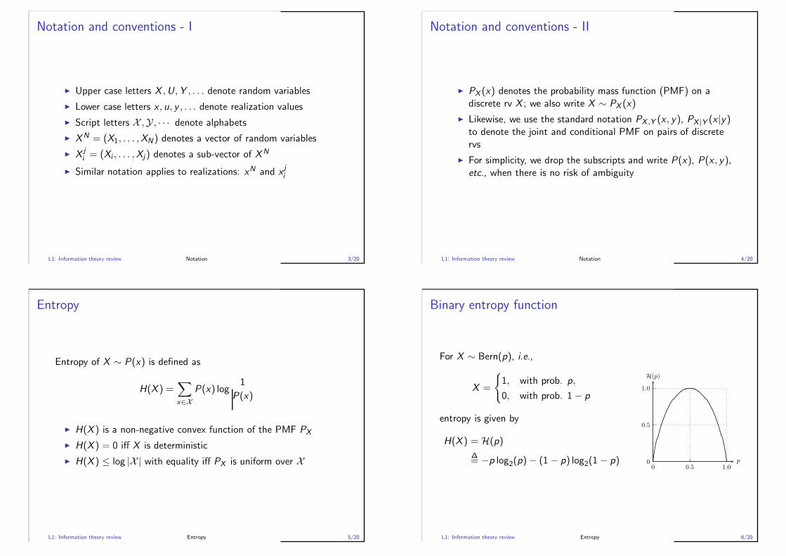
Binary entropy function
For X ∼ Bern(p), i.e.,
X =
{
1, with prob. p,
0, with prob. 1− p
entropy is given by
H(X ) = H(p)
∆= −p log2(p)− (1− p) log2(1− p) 0
0.5
1.0
0 0.5 1.0p
H(p)
L1: Information theory review Entropy 6/20

Joint Entropy
◮ Joint entropy of (X ,Y ) ∼ P(x , y)
H(X ,Y ) =∑
(x ,y)∈X×YP(x , y) log
1
P(x , y)
◮ Conditional entropy of X given Y
H(X |Y ) = H(X ,Y )− H(Y ) =∑
(x ,y)∈X×YP(x , y) log
1
P(x |y)
◮ H(X |Y ) ≥ 0 with eq. iff X if a function of Y
◮ H(X |Y ) ≤ H(X ) with eq. iff X and Y are independent
L1: Information theory review Entropy 7/20
Fano’s inequality
For any pair of jointly distributed rvs (X ,Y ) over a commonalphabet X , the “probability of error”
Pe∆= Pr(X 6= Y )
satisfies
H(X |Y ) ≤ H(Pe) + Pe log(|X | − 1) ≤ 1 + log |X |.
• Thus, if H(X |Y ) is bounded away from zero, so is Pe .
L1: Information theory review Entropy 8/20
Chain rule
◮ For any pair of rvs (X ,Y ),
◮ H(X ,Y ) = H(X ) + H(Y |X )
◮ H(X ,Y ) = H(Y ) + H(X |Y )
◮ H(X ,Y ) ≤ H(X ) + H(Y ) with equality iff X and Y areindependent.
L1: Information theory review Entropy 9/20
Chanin rule - II
For any random vector XN = (X1, . . . ,XN)
H(XN) = H(X1) + H(X2|X1) + · · · + H(XN |XN−1)
=
N∑
i=1
H(Xi |X i−1)
≤N∑
i=1
H(Xi )
with equality iff X1, . . . ,XN are independent.
L1: Information theory review Entropy 10/20

Mutual information
◮ For any (X ,Y ) ∼ P(x , y), the mutual information betweenthem is defined as
I (X ;Y ) = H(X )− H(X |Y ).
◮ Alternatively,
I (X ;Y ) = H(Y )− H(Y |Y )
orI (X ;Y ) = H(X ) + H(Y )− H(X ,Y )
L1: Information theory review Mutual information 11/20
Mutual information bounds
We have0 ≤ I (X ;Y ) ≤ min{H(X ),H(Y )}
with
◮ I (X ;Y ) = 0 iff X and Y are independent
◮ I (X ;Y ) = min{H(X ),H(Y )} iff X is a function of Y or viceversa
L1: Information theory review Mutual information 12/20
Conditional mutual information
◮ For any three-part ensemble (X ,Y ,Z ) ∼ P(x , y , z), themutual information between X and Y conditional on Z isdefined as
I (X ;Y |Z ) = H(X |Z )− H(X |YZ )
◮ Alternatively,
I (X ;Y |Z ) = H(Y |Z )−H(Y |YZ ) = H(X |Z )+H(Y |Z )−H(X ,Y |Z )
◮ Examples exist for both
I (X ;Y |Z ) < I (X ;Y ) and I (X ;Y |Z ) > I (X ;Y )
L1: Information theory review Mutual information 13/20
Chain rule of mutual information
For any ensemble (XN ,Y ) ∼ P(x1, . . . , xN , y), we have
I (XN ;Y ) = I (X1;Y ) + I (X2;Y |X1) + · · ·+ I (XN ;Y |XN−1)
=N∑
i=1
I (Xi ;Y |X i−1)
L1: Information theory review Mutual information 14/20
Data processing theorem
If X → Y → Z form a Markov chain, i.e., if P(z |yx) = P(z |y) forall x , y , z , then
I (X ;Z ) ≤ I (X ;Y ).
Proof: Use the chain rule to expand I (X ;YZ ) in two differentways.
I (X ;YZ ) = I (X ;Y ) + I (X ;Z |Y ) = I (X ;Y ) by Markov property
I (X ;YZ ) = I (X ;Z ) + I (X ;Y |Z ) ≥ I (X ;Z )
L1: Information theory review Mutual information 15/20
Discrete memoryless channels (DMC)
A DMC is a conditional probability assignment{W (y |x) : x ∈ X , y ∈ Y} for two discrete alphabets X , Y.
◮ We write W : X → Y or simply W to denote a DMC
◮ X is called the channel input alphabet
◮ Y is called the channel output alphabet
◮ W is called the channel transition probability matrix
L1: Information theory review Channel coding theorem 16/20
Channel coding
Channel coding is an operation to achieve reliable communicationover an unreliable channel. It has two parts.
◮ An encoder that maps messages to codewords
◮ A decoder that maps channel outputs back to messages
L1: Information theory review Channel coding theorem 17/20
Block code
Given a channel W : X → Y, a block code with length N and rateR is such that
◮ the message set consists of integers {1, . . . ,M = 2NR}◮ the codeword for each message m is a sequence xN(m) of
length N over XN
◮ the decoder operates on channel output blocks yN over YN
and produces estimates m of the transmitted message m.
◮ the performance is measured by the probability of frame(block) error, also called frame error rate (FER), which isdefined as
Pe = Pr(m 6= m)
where m is the transmitted message which is assumedequiprobable over the message set and m denotes the decoderoutput.
L1: Information theory review Channel coding theorem 18/20

Channel capacity
The capacity C (W ) of a DMC W : X → Y is defined as themaximum of I (X ;Y ) over all probability assignments of the form
PX ,Y (x , y) = Q(x)W (y |x)
where Q is an arbitrary probability assignment over the channelinput alphabet X , or briefly,
C (W ) = maxQ(x) I (X ;Y ).
L1: Information theory review Channel coding theorem 19/20
Channel capacity theorem
For any fixed rate R < C (W ) and ǫ > 0, there exist block codingschemes with rate R and Pe < ǫ provided the code block length Ncan be chosen as large as desired.
L1: Information theory review Channel coding theorem 20/20
L1: Information theory review
L2: Gaussian channel
L3: Algebraic coding
L4: Probabilistic coding
L5: Channel polarization
L6: Polar coding
L7: Origins of polar coding
L8: Coding for bandlimited channels
L9: Polar codes for selected applications
L2: Gaussian channel 1/34
Lecture 2 – Additive White Gaussian Noise (AWGN)
channel
◮ Objective: Review the basic AWGN channel
◮ Topics
◮ Discrete-time and continuous-time Gaussian channel
◮ Signaling over a Gaussian channel
◮ The union bound
◮ Reference for this part: David Forney, Lecture Notes forCourse 6.452 Principles of Digital Communication II, Spring2005, Available online: http://ocw.mit.edu.
L2: Gaussian channel Outline 2/34
Discrete-time (DT) AWGN channel
The input at time i is a real number xi , the output is given by
yi = xi + zi
where the noise sequence {zi} over the entire time frame is iidGaussian ∼ N(0, σ2).
L2: Gaussian channel Capacity 3/34
Capacity of the DT-AWGN channel
If a block code {xN(m) : 1 ≤ m ≤ M} is employed subject to a“power constraint”
N∑
i=1
x2i (m) ≤ NP , 1 ≤ m ≤ M,
the capacity is given by
C =1
2log2
(
1 +P
σ2
)
bits.
L2: Gaussian channel Capacity 4/34
Continuous-time (CT) AWGN channel
This is a waveform channel whose output is given by
y(t) = x(t) + w(t)
where x(t) is the channel input and w(t) is white Gaussian noisewith power spectral density No/2.
L2: Gaussian channel Capacity 5/34
Capacity of the CT-AWGN channel
If signaling over the CT-AWGN channel is restricted to waveforms{x(t) that are time-limited to [0,T ], band-limited to [−W ,W ],and power-limited to P , i.e.,
∫ T
0x2(t)dt ≤ PT ,
then the capacity is given by
C[b/s] = W log2
(
1 +P
NoW
)
bits/sec.
L2: Gaussian channel Capacity 6/34
DT model for the CT-AWGN model◮ By Nyquist theory, each use of the CT-AWGN channel with
signals of duration T and bandwidth W gives rise to 2WTindependent DT-AWGN channels.
◮ It is customary to use the DT channels in pairs of “in-phase”and “quadrature” components of a complex number
◮ Accordingly, the capacity of the two-dimensional (2D)DT-AWGN channels derived from a CT-AWGN channel aregiven by
C2D = log2
(
1 +Es
No
)
bits/2D or bits/Hz
where Es is the signal energy per 2D,
Es∆=
P
2W= PT J/2D or J/Hz.
L2: Gaussian channel Capacity 7/34
Signal-to-Noise Ratio
◮ Primary parameters in an AWGN channel are: Signalbandwidth W (Hz), signal power P (Watt), noise powerspectral density N0/2 (Joule/Hz).
◮ Capacity equals C[b/s] = W log2(1 + P/N0W ).
◮ Define SNR∆= P/N0W to write C[b/s] = W log2(1 + SNR).
◮ Writing SNR = (P/2W )/(N0/2), SNR can be interpreted asthe signal energy per real dimension divided by the noiseenergy per real dimension.
◮ For 2D complex signalling, one may write SNR = (P/W )/N0
and interpret SNR as signal energy per 2D divided by thenoise energy per 2D.
L2: Gaussian channel Signalling 8/34
Signal energy per 2D: Es
◮ Definition: Es∆= P/W (joules)
◮ Es can be interpreted as signal energy per two dimensions.
◮ For 2D (complex) signalling Es is the signal energy.
◮ For 1D (real) signalling, Es/2 is the energy per signal.
◮ Note that SNR = Es/N0 and one may write
C[b/2D] = log2(1 + Es/N0)
L2: Gaussian channel Signalling 9/34
Spectral efficiency ρ and data rate R
◮ ρ is defined as the number of bits per two dimension over theAWGN channel. Units: bits/two-dimension or b/2D.
◮ R is defined as the number of bits per second sent over theAWGN channel. Units: bits/sec or b/s.
◮ Since there are W (2D/s) 2D dimensions per second, we have
R = ρW .
◮ Since ρ = R/W , the units of ρ can also be expressed asb/s/Hz (bits per second per Hertz).
L2: Gaussian channel Signalling 10/34

Normalized SNR◮ Shannon’s law says that for reliable communication one has to
haveρ < log2(1 + SNR)
orSNR > 2ρ − 1.
◮ This motivates the definition
SNRnorm∆=
SNR
2ρ − 1.
◮ Shannon limit now reads
SNRnorm > 1 (0dB).
◮ The value of SNRnorm (in dB) for an operational systemmeasures “gap to capacity”, indicating how much room thereis for improvement.
L2: Gaussian channel Signalling 11/34
Another measure of signal-to-noise ratio: Eb/N0
◮ Energy per bit is defined as
Eb∆= Es/ρ,
and signal-to-noise ratio per information bit as
Eb/N0∆= Es/ρN0 = SNR/ρ.
◮ Shannon’s limit can be written in terms of Eb/N0 can bewritten as
Eb/N0 >2ρ − 1
ρ.
◮ The function (2ρ − 1)/ρ is an increasing function of ρ > 0,and as ρ → 0, approaches ln 2 ≈ 0.69 (1.59 dB), which iscalled the ultimate Shannon limit on Eb/N0.
L2: Gaussian channel Signalling 12/34
Power-limited and band-limited regimes
◮ Operation over an AWGN channels is classified as“power-limited” if SNR ≪ 1 and “band-limited” if SNR ≫ 1.
◮ The Shannon limit on the spectral efficiency can beapproximated as
ρ < log2(1 + SNR) ≈{
SNR log2 e, SNR ≪ 1;
log2 SNR , SNR ≫ 1.
◮ In the power-limited regime, the Shannon limit on ρ isdoubled by doubling the SNR (a 3 dB increase); while in theband-limited case, doubling the SNR increases the Shannonlimit by only 1 b/2D.
L2: Gaussian channel Signalling 13/34
Band-limited regime
−10 −5 0 5 10 15 20 25 30 35 400
5
10
15
20
25
SNR (dB)
Cap
acity
(b/
s)
Capacity and Bandwidth Tradeoff
W = 1W = 2
Band−limitedregime
◮ Doubling the bandwidth almost doubles the capacity in thedeep band-limited regime.
◮ Doubling the bandwidth has small effect if the SNR is low(power-limited regime).
L2: Gaussian channel Signalling 14/34
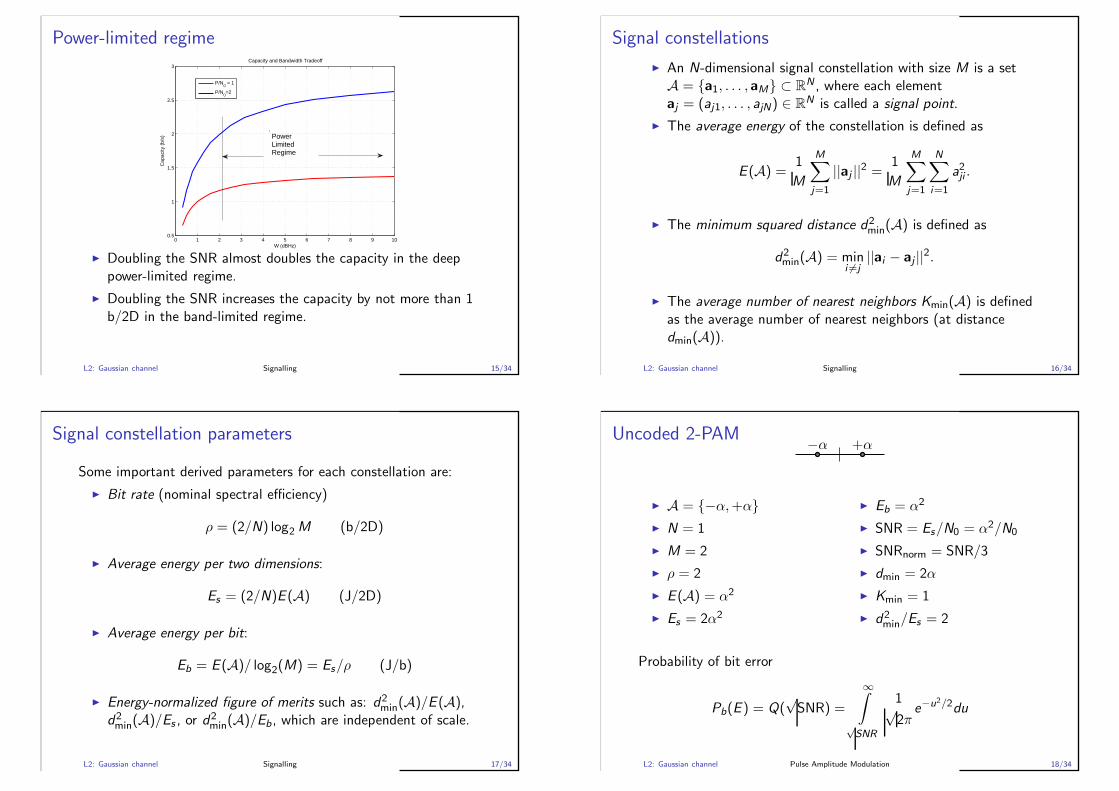
Power-limited regime
0 1 2 3 4 5 6 7 8 9 100.5
1
1.5
2
2.5
3
W (dBHz)
Cap
acity
(b/
s)
Capacity and Bandwidth Tradeoff
P/N0 = 1
P/N0=2
PowerLimitedRegime
◮ Doubling the SNR almost doubles the capacity in the deeppower-limited regime.
◮ Doubling the SNR increases the capacity by not more than 1b/2D in the band-limited regime.
L2: Gaussian channel Signalling 15/34
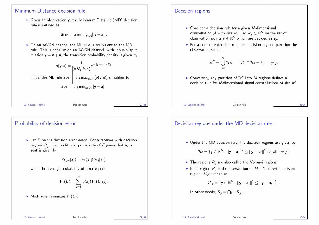
Signal constellations
◮ An N-dimensional signal constellation with size M is a setA = {a1, . . . , aM} ⊂ R
N , where each elementaj = (aj1, . . . , ajN) ∈ R
N is called a signal point.
◮ The average energy of the constellation is defined as
E (A) =1
M
M∑
j=1
||aj ||2 =1
M
M∑
j=1
N∑
i=1
a2ji .
◮ The minimum squared distance d2min(A) is defined as
d2min(A) = min
i 6=j||ai − aj ||2.
◮ The average number of nearest neighbors Kmin(A) is definedas the average number of nearest neighbors (at distancedmin(A)).
L2: Gaussian channel Signalling 16/34
Signal constellation parameters
Some important derived parameters for each constellation are:
◮ Bit rate (nominal spectral efficiency)
ρ = (2/N) log2 M (b/2D)
◮ Average energy per two dimensions:
Es = (2/N)E (A) (J/2D)
◮ Average energy per bit:
Eb = E (A)/ log2(M) = Es/ρ (J/b)
◮ Energy-normalized figure of merits such as: d2min(A)/E (A),
d2min(A)/Es , or d
2min(A)/Eb , which are independent of scale.
L2: Gaussian channel Signalling 17/34
Uncoded 2-PAM −α +α
◮ A = {−α,+α}◮ N = 1
◮ M = 2
◮ ρ = 2
◮ E (A) = α2
◮ Es = 2α2
◮ Eb = α2
◮ SNR = Es/N0 = α2/N0
◮ SNRnorm = SNR/3
◮ dmin = 2α
◮ Kmin = 1
◮ d2min/Es = 2
Probability of bit error
Pb(E ) = Q(√SNR) =
∞∫
√SNR
1√2π
e−u2/2du
L2: Gaussian channel Pulse Amplitude Modulation 18/34

Uncoded 2-PAM
−2 0 2 4 6 8 10 1210
−6
10−5
10−4
10−3
10−2
10−1
100
Eb/N
0 (dB)
Pb(E
)
Uncoded 2−PAM
Uncoded 2−PAMUltimate Shannon limitShannon limit at ρ = 2
Coding Gain 7.8 dB
◮ Spectral efficiency: ρ = 2 b/2D
◮ Shannon limit: Eb/N0 > (2ρ − 1)/ρ = 3/2 (1.76 dB)
◮ Target Pb(E ) = 10−5 achieved at Eb/N0 = 9.6 dB
◮ Potential coding gain is 9.6 − 1.76 = 7.84 dB
◮ Ultimate coding gain is 9.6− (−1.59) = 10 dB with ρ → 0
L2: Gaussian channel Pulse Amplitude Modulation 19/34
Uncoded M-PAM
◮ Signal set: A = α{±1,±3, . . . ,±(M − 1)}◮ Parameters:
◮ ρ = 2 log2 M b/2D
◮ E (A) = α2(M2 − 1)/3 J/D
◮ Es = 2E (A) = 2α2(M2 − 1)/3 J/2D
◮ SNR = Es/N0 = 2α2(M2 − 1)/3N0
◮ SNRnorm = SNR/(2ρ − 1) = 2α2/3
◮ Probability of symbol error, Ps(E ), is given by
Ps(E ) =2(M − 1)
MQ(α/σ) ≈ 2Q(α/σ) = 2Q(
√
3SNRnorm)
where σ =√
N0/2.
L2: Gaussian channel Pulse Amplitude Modulation 20/34
Uncoded M-PAM Performance
0 1 2 3 4 5 6 7 8 9 1010
−6
10−5
10−4
10−3
10−2
10−1
100
SNRnorm
(dB)
Ps(E
)
Uncoded M−PAM, M>>1
Uncoded PAMShannon limit
◮ This curve is valid for any M-PAM with M ≫ 1.
◮ Target Ps(E ) = 10−5 is achieved at SNRnorm = 8.1 dB.
◮ Shannon limit is SNRnorm = 0 dB.L2: Gaussian channel Pulse Amplitude Modulation 21/34
Uncoded 4-QAM
A = {(−α,−α), (−α,α), (α,−α), (α,α)}. Parameters:◮ N = 2◮ M = 4◮ ρ = 2◮ E (A) = 2α2
◮ Es = 2α2
◮ Eb = α2
◮ dmin = 2α◮ Kmin = 2◮ d2
min/Es = 2
L2: Gaussian channel Quadrature Amplitude Modulation 22/34

Uncoded M ×M-QAM
◮ The signal constellation is A = AM-PAM ×AM-PAM
◮ Parameters:
◮ ρ = log2 M2 = 2 log2 M b/2D
◮ E (A) = 2α2(M2 − 1)/3 J/2D
◮ Es = E (A) = 2α2(M2 − 1)/3 J/2D
◮ SNR = Es/N0 = 2α2(M2 − 1)/3N0
◮ SNRnorm = SNR/(2ρ − 1) = 2α2/3
◮ Probability of symbol error, Ps(E ), is given by (see notes)
Ps(E ) ≈ 4Q(√
3SNRnorm)
L2: Gaussian channel Quadrature Amplitude Modulation 23/34
Uncoded QAM performance
0 1 2 3 4 5 6 7 8 9 1010
−6
10−5
10−4
10−3
10−2
10−1
100
SNRnorm
(dB)
Ps(E
)
Uncoded QAM
Uncoded QAMShannon limit
◮ Curve valid for M ×M-QAM with M ≫ 1.
◮ Target Ps(E ) = 10−5 achieved at SNRnorm = 8.4 dB.
◮ Gap to Shannon limit is 8.4 dB.L2: Gaussian channel Quadrature Amplitude Modulation 24/34
Cartesian product constellations◮ Given a constellation A, define a new constellation A′ as the
K th Cartesian power of A:
A′ = AK = A×A× · · · × A︸ ︷︷ ︸
K
◮ E.g., 4−QAM is the second Cartesian power of 2− PAM.
◮ The parameters of A′ are related to those of A as follows:
◮ N ′ = KN
◮ M ′ = MK
◮ E (A′) = K E (A)
◮ K ′
min = K Kmin
◮ E ′
s = Es
◮ E ′
b = Eb
◮ d ′
min = dmin
◮ ρ′ = ρ
L2: Gaussian channel Quadrature Amplitude Modulation 25/34
MAP and ML decision rules◮ Consider transmission over an AWGN channel using a
constellation A = {a1, . . . , aM}. Suppose in each use of thesystem a signal aj ∈ A is selected with probability p(aj) andsent over the channel.
◮ Given the channel output y, the receiver needs to makes adecision a on which of the signal points aj was sent. Thereare various decision rules.
◮ The Maximum A-Posteriori Probability (MAP) rule sets
aMAP = argmaxa∈A[p(a|y)] = argmaxa∈A[p(a)p(y|a)/p(y)].
◮ The Maximum Likelihood (ML) rule sets
aML = argmaxa∈A[p(y|a)].
◮ ML and MAP rules are equivalent for the important specialcase where p(aj) = 1/M for all j .
L2: Gaussian channel Decision rules 26/34
Minimum Distance decision rule
◮ Given an observation y, the Minimum Distance (MD) decisionrule is defined as
aMD = argmina∈A||y − a||.
◮ On an AWGN channel the ML rule is equivalent to the MDrule. This is because on an AWGN channel, with input-outputrelation y = a+n, the transition probability density is given by
p(y|a) = 1
(πN0)N/2)e−||y−a||2/N0 .
Thus, the ML rule aML = argmaxa∈A[p(y|a)] simplifies to
aML = argmina∈A||y − a||.
L2: Gaussian channel Decision rules 27/34
Decision regions
◮ Consider a decision rule for a given N-dimensionalconstellation A with size M. Let Rj ⊂ R
N be the set ofobservation points y ∈ R
N which are decided as aj .
◮ For a complete decision rule, the decision regions partition theobservation space:
RN =
M⋃
j=1
Rj ; Rj ∩Ri = ∅, i 6= j .
◮ Conversely, any partition of RN into M regions defines adecision rule for N-dimensional signal constellations of size M.
L2: Gaussian channel Decision rules 28/34
Probability of decision error
◮ Let E be the decision error event. For a receiver with decisionregions Rj , the conditional probability of E given that aj issent is given by
Pr(E |aj ) = Pr(y /∈ Rj |aj),
while the average probability of error equals
Pr(E ) =
M∑
j=1
p(aj) Pr(E |aj).
◮ MAP rule minimizes Pr(E ).
L2: Gaussian channel Decision rules 29/34
Decision regions under the MD decision rule
◮ Under the MD decision rule, the decision regions are given by
Rj = {y ∈ RN : ||y − aj ||2 ≤ ||y − ai ||2 for all i 6= j}
◮ The regions Rj are also called the Voronoi regions.
◮ Each region Rj is the intersection of M − 1 pairwise decisionregions Rji defined as
Rji = {y ∈ RN : ||y − aj ||2 ≤ ||y − ai ||2}.
In other words, Rj =⋂
i 6=j Rji .
L2: Gaussian channel Decision rules 30/34
Probability of error under MD rule on AWGN
◮ Under any rigid motion (translation or rotation) of aconstellation A, the Voronoi regions also move in the sameway.
◮ Under the MD decision rule, on any additive AWGN channelwe have
Pr(E |aj) = 1−∫
Rj
p(y|aj )dy = 1−∫
Rj−aj
pN(n)dn
This probability of error is invariant under rigid motions.(Proof is left as exercise.) (Is this true for any additive noise?)
◮ Likewise, Pr(E ) is invariant under rigid motions.
◮ If the mean m = 1M
∑
j aj of a constellation A is not zero, wemay translate it by −m to reduce the mean energy from E (A)to E (A)− ||m||2 without changing Pr(E ).
L2: Gaussian channel Decision rules 31/34
Probability of decision error for some constellations
◮ For 2-PAMPr(E ) = Q(
√
2Eb/N0)
where Q(x) =∫∞x
1√2πe−u2/2du.
◮ For 4-QAM
Pr(E ) = 1− (1− Q(√
2Eb/N0))2 ≈ 2Q(
√
2Eb/N0).
◮ One can express exact error probabilities for M-PAM and(M ×M)-QAM in terms of the Q function. (Exercise)
◮ However, for general constellations it becomes impractical todetermine the exact error probability. Often one uses somebounds and approximations instead of the exact forms.
L2: Gaussian channel Decision rules 32/34
Pairwise error probabilities
We consider MD decision rules and AWGN channels here.
◮ The pairwise error probability Pr(aj → ai ) is defined as theprobability that, conditional on aj being transmitted, thereceived point y is closer to ai than to aj . In other words
Pr(aj → ai ) = Pr(||y − ai || ≤ ||y − aj || | aj)
◮ Recalling the pairwise error regions
Rji = {y ∈ RN : ||y − aj ||2 ≤ ||y − ai ||2},
it can be shown that
Pr(aj → ai) =1√πN0
∫ ∞
d(ai ,aj)/2e−x2/N0dx = Q
( ||ai − aj ||√2N0
)
.
L2: Gaussian channel Union bound 33/34
The union bound◮ The conditional probability of error is bounded (under the MD
decision rule on an AWGN channel) as
Pr(E |aj ) ≤∑
i 6=j
Pr(aj → ai) =∑
i 6=j
Q
( ||ai − aj ||√2N0
)
.
◮ This leads to
Pr(E ) ≤ 1
M
M∑
j=1
∑
i 6=j
Q
( ||ai − aj ||√2N0
)
.
◮ One may also use the approximation
Pr(E ) ≈ Kmin(A)Q
(dmin(A)√
2N0
)
.
◮ The union bound is tight at sufficiently high SNR.
L2: Gaussian channel Union bound 34/34
L1: Information theory review
L2: Gaussian channel
L3: Algebraic coding
L4: Probabilistic coding
L5: Channel polarization
L6: Polar coding
L7: Origins of polar coding
L8: Coding for bandlimited channels
L9: Polar codes for selected applications
L3: Algebraic coding 1/35
Lecture 3 – Algebraic coding
◮ Objective: Introduce the rationale for coding, discuss someimportant algebraic codes
◮ Topics
◮ Why coding?
◮ Some important algebraic codes
◮ Reed-Muller codes
◮ Reed-Solomon codes
◮ BCH codes
L3: Algebraic coding 2/35
Motivation for coding
◮ Simple contellations such as PAM and QAM are far fromdelivering Shannon’s promise. They have a large gap toShannon limit.
◮ Signaling schemes such as orthogonal, bi-orthogonal, simplexachieve Shannon capacity when one can expand thebandwidth indefinitely; however, after a certain point theybecome impractical both in terms of complexity per bit andbandwidth limitations.
◮ Shannon’s proof shows that in the power-limited regime, thekey to achieving capacity is to begin with a simple 1D or 2Dconstellation A, consider Cartesian powers AN of increasinglyhigh orders, and select a subset A′ ⊂ AN to improve theminimum distance of the constellation at the expense ofspectral efficiency.
L3: Algebraic coding Motivation 3/35
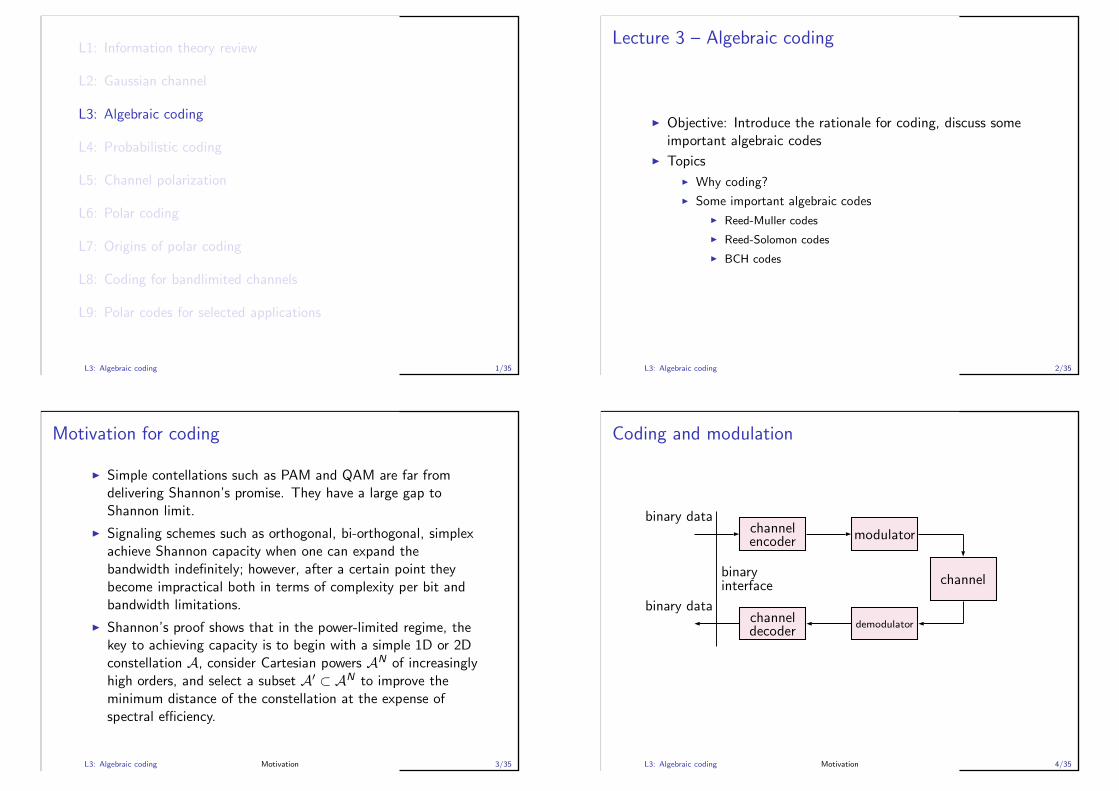
Coding and modulation
binary datachannelencoder modulator
channel
binary datachanneldecoder
demodulator
binaryinterface
L3: Algebraic coding Motivation 4/35
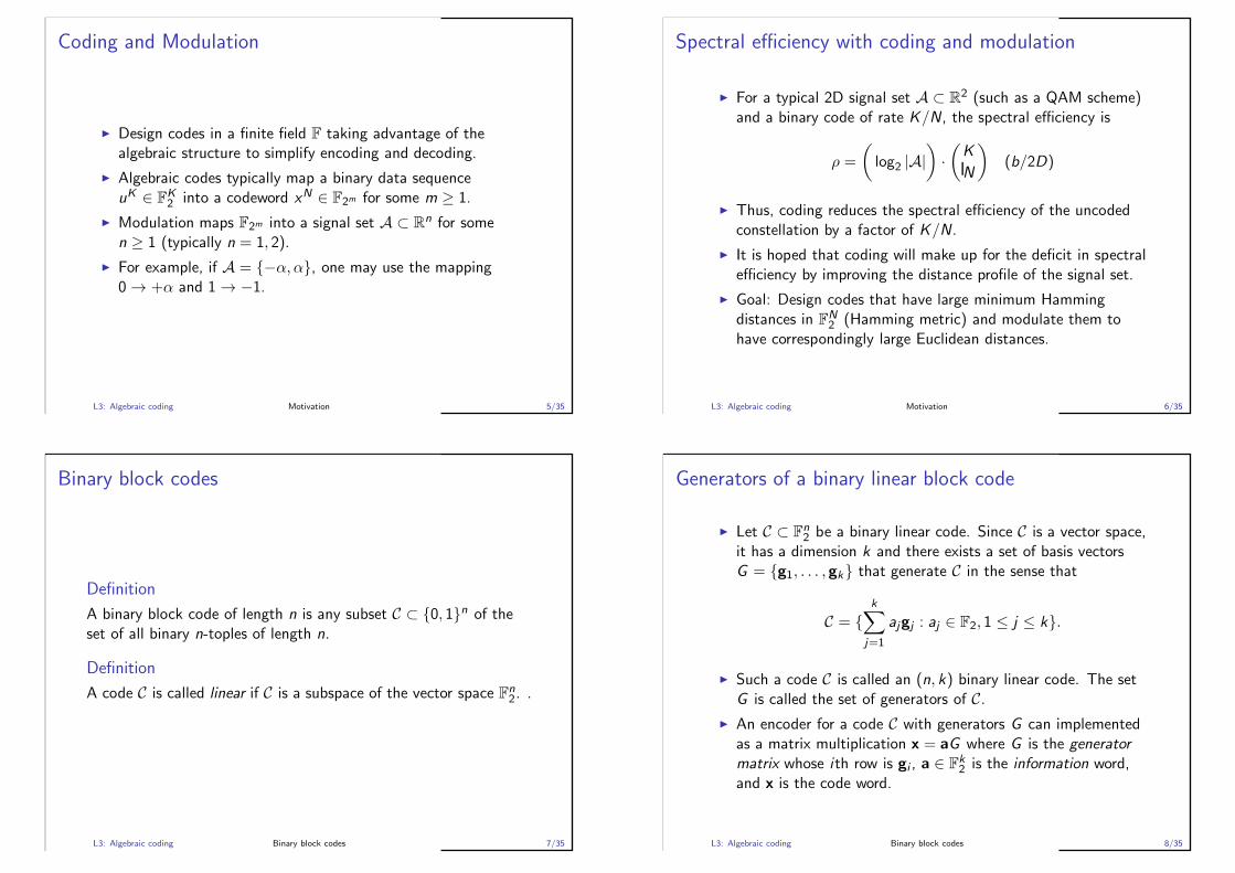
Coding and Modulation
◮ Design codes in a finite field F taking advantage of thealgebraic structure to simplify encoding and decoding.
◮ Algebraic codes typically map a binary data sequenceuK ∈ F
K2 into a codeword xN ∈ F2m for some m ≥ 1.
◮ Modulation maps F2m into a signal set A ⊂ Rn for some
n ≥ 1 (typically n = 1, 2).
◮ For example, if A = {−α,α}, one may use the mapping0 → +α and 1 → −1.
L3: Algebraic coding Motivation 5/35
Spectral efficiency with coding and modulation
◮ For a typical 2D signal set A ⊂ R2 (such as a QAM scheme)
and a binary code of rate K/N, the spectral efficiency is
ρ =
(
log2 |A|)
·(K
N
)
(b/2D)
◮ Thus, coding reduces the spectral efficiency of the uncodedconstellation by a factor of K/N.
◮ It is hoped that coding will make up for the deficit in spectralefficiency by improving the distance profile of the signal set.
◮ Goal: Design codes that have large minimum Hammingdistances in F
N2 (Hamming metric) and modulate them to
have correspondingly large Euclidean distances.
L3: Algebraic coding Motivation 6/35
Binary block codes
Definition
A binary block code of length n is any subset C ⊂ {0, 1}n of theset of all binary n-toples of length n.
Definition
A code C is called linear if C is a subspace of the vector space Fn2. .
L3: Algebraic coding Binary block codes 7/35
Generators of a binary linear block code
◮ Let C ⊂ Fn2 be a binary linear code. Since C is a vector space,
it has a dimension k and there exists a set of basis vectorsG = {g1, . . . ,gk} that generate C in the sense that
C = {k∑
j=1
ajgj : aj ∈ F2, 1 ≤ j ≤ k}.
◮ Such a code C is called an (n, k) binary linear code. The setG is called the set of generators of C.
◮ An encoder for a code C with generators G can implementedas a matrix multiplication x = aG where G is the generatormatrix whose ith row is gi , a ∈ F
k2 is the information word,
and x is the code word.
L3: Algebraic coding Binary block codes 8/35
The Hamming weight
Definition
For x ∈ Fn2, the Hamming weight of x is defined as
wH(x) = number of ones in x
The Hamming weight has the following properties:
◮ Non-negativity: wH(x) ≥ 0 with equality iff x = 0.
◮ Symmetry: wH(−x) = wH(x).
◮ Triangle inequality: wH(x+ y) ≤ wH(x) + wH(y).
L3: Algebraic coding Binary block codes 9/35
The Hamming distance
Definition
For x, y ∈ Fn2, the Hamming distance between x and y is defined as
dH(x, y) = wH(x− y)
The Hamming distance has the following properties for anyx, y, z ∈ F
n2:
◮ Non-negativity: dH(x, y) ≥ 0 with equality iff x = y.
◮ Symmetry: dH(x, y) = dH(y, x).
◮ Triangle inequality: dH(x, y) ≤ dH(x, z) + dH(z, y).
Thus, the Hamming distance is a metric in the mathematical senseof the word and the space F
n2 with this metric is called the
Hamming space.
L3: Algebraic coding Binary block codes 10/35
Distance invariance
Theorem
The set of Hamming distance dH(x, y) from any codeword x ∈ Cto all codewords y ∈ C is independent of x, and is equal to the setof Hamming weights wH(y) of all codewords y ∈ C.
Proof.
The set of distances from x is {dH(x, y) : y ∈ C}. This set can bewritten as {wH(x+ y : y ∈ C} = x+ C. But x+ C = C for a linearcode (why?). Taking x = 0, we obtain the proof.
L3: Algebraic coding Binary block codes 11/35
Minimum distance
Definition
The code minimum distance d of a code C is defined as theminimum of d(x, y) over all x, y ∈ C with x 6= y.
Remark
The minimum distance d equals the minimum of wH(x over allnon-zero codewords x ∈ C.
Remark
We refer to an (n, k) code with minimum distance d as an(n, k , d) code. For example, an (n, 1) repetition code has d = nand is an (n, 1, d) code.
L3: Algebraic coding Binary block codes 12/35

Euclidean Images of Binary Codes
Binary codes C are mapped to signal constellations by the mapping
s : Fn2 → R
n
which takes x → s so that
si =
{
+α, if xi = 0,
−α, if xi = 1.
L3: Algebraic coding Coding gain 13/35
Minimum distances
◮ When a code C is mapped to a signal constellation s(C) bythe mapping s defined above, the Hamming distancestranslate to Euclidean distances as follows:
||s(x) − s(y)||2 = 4α2dH(x, y)
◮ Thus, minimum code distance translates to a minimum signaldistance of
d2min(s(C)) = 4α2dH(C) = 4α2d .
L3: Algebraic coding Coding gain 14/35
Nominal coding gain, union bound
◮ When a code C is mapped to a signal constellation s(C), thenominal coding gain of the constellation is given by
γc(s(C)) =d2min(s(C))4Eb
=kd
n
◮ Every signal has the same number of nearest neighborsKmin(x) = Nd .
◮ Union bound:
Pb(E ) ≈ Kb/s(C))Q(√
γc(s(C))2Eb/N0
)
=Nd
kQ(√
2d R Eb/N0
)
where R = k/n is the code rate.
L3: Algebraic coding Coding gain 15/35
Decision rules
◮ Minimum distance (MD) decoding. Given a received vectorr ∈ R
n, find the signal point s(x) over all x ∈ C such that||r − s(x)||2 is minimized.
◮ Hard-decision decoding. Given a received vector r ∈ Rn,
quantize r into y ∈ F n2 and find the codeword x ∈ C closest to
y in the Hamming metric.
◮ Erasure-and-error decoding. Map the received word r into aword y ∈ {0, 1, ?}n and find the codeword x closest to y
ignoring the erased coordinates (where yk =?).
◮ Generalized minimum distance (GMD) decoding. Applyerasures and errors decoding by erasing successivelys = d − 1, d − 3, . . . positions, using the reliability metric |rk |to prioritize erasure locations. Pick the best candidate.
L3: Algebraic coding Coding gain 16/35

Hard-decision decoding
Hard-decisions are obtained by the mapping r → y such that
y =
{
0, r > 0,
1, r ≤ 0.
L3: Algebraic coding Coding gain 17/35
Performance of some early codes◮ Performance of some well-known codes under with
hard-decision decoding.
◮ Performance limited both by the short block length andhard-decision decoding.
L3: Algebraic coding Coding gain 18/35
Reed-Muller codes (Reed, 1954), (Muller, 1954)
◮ For every m ≥ 0 and 0 ≤ r ≤ m, there exists an RM codeRM(r ,m).
◮ Define the RM codes with extreme parameters as follows.
◮ RM(m,m)∆= {0, 1}n with (n, k , d) = (2m, 2m, 1).
◮ RM(0,m)∆= {0n, 1n} with (n, k , d) = (2m, 1, n).
◮ RM(−1,m)∆= {0n} with (n, k , d) = (2m, 0,∞).
◮ Define the remaining RM codes for m ≥ 1 and 0 ≤ r ≤ mrecursively by
RM(r ,m) = {(u,u+v)|u ∈ RM(r ,m−1), v ∈ RM(r−1,m−1)}.
◮ This construction of RM codes is called the Plotkinconstruction.
L3: Algebraic coding Reed-Muller codes 19/35
Generator matrices of RM codes
◮ Let
U1∆=
[1 01 1
]
, Um∆=
[Um−1 0Um−1 Um−1
]
, m ≥ 2.
The generator matrix of RM(r ,m) is the submatrix of Um
consisting of rows of Hamming weight 2r or greater.
◮ For any m ≥ 1, the matrix Um has( (m
), r) rows with
Hamming weight 2m−r , 0 ≤ r ≤ m.
L3: Algebraic coding Reed-Muller codes 20/35

Properties of RM codes
◮ RM(r ,m) is a binary linear block code with parameters withparameters (n, k , d) = (2m,
∑ri=0
(ri
), 2m−r ).
◮ The dimensions satisfy the relation
k(r ,m) = k(r ,m − 1) + k(r − 1,m − 1).
◮ The codes are nested: RM(r − 1,m) ⊂ RM(r ,m).
◮ The minimum distance of RM(r ,m) is d = 2m−r if r ≥ 0.
◮ No of nearest neighbors is given by
Nd = 2r∏
0≤i≤m−r−1
2m−i − 1
2m−r−i − 1.
L3: Algebraic coding Reed-Muller codes 21/35
Tableaux of RM codes
(Figure credit: Forney and Costello, Proc. IEEE, June 2007.)
L3: Algebraic coding Reed-Muller codes 22/35
Coding gains of various RM codes
◮ RM(m − 1,m) are single parity-check codes with nominalcoding gains 2k/n which goes to 2 (3 dB) as n → ∞.However, Nd = 2m(2m − 1)/2 and Kb = 2m−1, which limitsthe coding gain.
◮ RM(m − 2,m) are Hamming codes extended by an overallparity. These codes have d = 4. The nominal coding gain is4k/n which goes to 6 dB as n → ∞. The actual coding gainis severely limited since Nd = 2m(2m − 1)/24 and Kb → ∞.
◮ RM(1,m) (first-order RM codes) have parameters(2m,m + 1, 2m−1). They have a nominal coding gain of(m + 1)/2, which goes to infinity. These codes can achievethe Shannon limit as m → ∞. RM(1,m) generates thebi-orthogonal signal set of dimension 2m and size 2m+1.
L3: Algebraic coding Reed-Muller codes 23/35
Reed-Muller coding gains
L3: Algebraic coding Reed-Muller codes 24/35

Decoding algorithms for RM codes
◮ Majority-logic decoding (Reed, 1964): A form ofsuccessive-cancellation (SC) decoding. Sub-optimal but fast.
◮ Soft-decision SC decoding (Schnabl-Bossert, 1995): Superiorto Reed’s algorithm, but slower.
◮ ML decoding by using trellis representations: Feasible forsmall code sizes.
L3: Algebraic coding Reed-Muller codes 25/35
Linear codes over finite fields
◮ An (n, k) linear code C over a finite field Fq is a k-dimensionalsubspace of the vector space F n
q = (Fq)n of all n-tuples over
Fq. For q = 2, this reduces to our previous definition of binarylinear codes.
◮ As a linear subspace C has k linearly independent codewords(g1, . . . ,gk) that generate C, in the sense that
C = {k∑
j=1
ajgj : aj ∈ Fq, 1 ≤ j ≤ k}
Thus C has qk distinct codewords.
L3: Algebraic coding Reed-Solomon codes 26/35
Reed-Solomon (RS) codes
◮ Introduced by Irving S. Reed and Gustave Solomon in 1960
◮ Can be defined over any field Fq
◮ A (n, k) RS code over Fq exists for any 0 ≤ k ≤ n ≤ q
◮ Encoding: Given k data symbols (f0, . . . , fk−1) over Fq,
◮ form the polynomial
f (z) = f0 + f1z + · · ·+ fk−1zk−1
◮ evaluate f (z) at each field element βi , 1 ≤ i ≤ q, namely,
compute f (βi ) =∑k−1
j=0 fjβji , to obtain the code symbols
(f (β1), . . . , f (βq))
◮ truncate if necessary to obtain a code of length n < q
L3: Algebraic coding Reed-Solomon codes 27/35
Properties of RS codes
◮ Minimum distance separable (MDS): A (n, k) RS code hasdmin = n− k , meeting the Singleton bound with equality
◮ Typically constructed over Fq with q = 2m with each symbolconsisting of m bits
◮ Very effective against correcting burst errors confined to asmall number of symbols
◮ Major applications: Consumer electronics, outer code inconcatenated coding schemes
◮ Decoding is usually by hard-decision:
◮ Berlekamp-Massey algorithm can correct any pattrern oft ≤ n− k errors
◮ Sudan-Guruswami (1999) algorithm can go beyond theminimum distance bound
L3: Algebraic coding Reed-Solomon codes 28/35

RS code application: G.975 optical transmission standard
◮ ITU-T G.975 standard (year 2000) for long-distancesubmarine optical transmission systems specified RS(255,239)code as the forward error correction (FEC) method.
◮ In bits, this is a (2040, 1912) code with rate R = 0.9373.
◮ This RS code has dmin = 16 (in bytes) and can correct anypattern of 8 byte errors.
◮ The BER requirement in this application is 10−12
◮ Data throughput 1 - 100 Gbps are supported
◮ G.975 RS codes continue to serve but are being supersededlately by more powerful proprietary solutions (“3rd GenerationFEC”) that use soft-decision decoders and provide bettercoding gains with higher redundancy
L3: Algebraic coding Reed-Solomon codes 29/35
Performance of RS(255,239) code
BER performance under hard-decision decoding
0 1 2 3 4 5 6 7 8 9 10 11 12 13 14 15
Eb/N
0 (dB)
10-15
10-14
10-13
10-12
10-11
10-10
10-9
10-8
10-7
10-6
10-5
10-4
10-3
10-2
10-1
100
BE
R
RS(255,239)Uncoded
L3: Algebraic coding Reed-Solomon codes 30/35
Performance of RS(255,239) code
Input BER vs output BER
10-4 10-3 10-2 10-1
Input BER
10-15
10-14
10-13
10-12
10-11
10-10
10-9
10-8
10-7
10-6
10-5
10-4
10-3
10-2
10-1
100
Out
put B
ER
RS(255,239)
L3: Algebraic coding Reed-Solomon codes 31/35
RS coding with concatenation
Over memoryless channels such as the AWGN channel powerfulcodes may be obtained by concatenating an inner code consistingof q = 2m codewords or signal points with an outer code over Fq.
The inner code is typically a binary block or convolutional code.The outer code is typically an RS code.
L3: Algebraic coding Concatenated coding 32/35
Interleaving
In a concatenated coding scheme an error in the inner codeappears as a burst of errors to the outer code. To make the symbolerrors made by the inner decoder look memoryless “interleaving” isused. A two dimensional array is prepared where outer coding isapplied on the rows and inner coding is applied on the columns.
When an error occurs in the inner code, a column is affected,which appears only as a single symbol error in the outer code.
L3: Algebraic coding Concatenated coding 33/35
RS concatenated code application: NASA standard
◮ In 1970s NASA used an RS/CC concatenated code
◮ The inner code is a CC with rate-1/2 and 64 states
◮ The outer code is an RS(255,223) code over F256
◮ The code has an overall code rate 0.437 and a coding gain of7.3 dB at 10−6
L3: Algebraic coding Concatenated coding 34/35
Performance of NASA concatenated code
(Figure credit: Forney and Costello, Proc. IEEE, June 2007.)
L3: Algebraic coding Concatenated coding 35/35
L1: Information theory review
L2: Gaussian channel
L3: Algebraic coding
L4: Probabilistic coding
L5: Channel polarization
L6: Polar coding
L7: Origins of polar coding
L8: Coding for bandlimited channels
L9: Polar codes for selected applications
L4: Probabilistic coding 1/40

Lecture 4 – Probabilistic approach to coding
◮ Objective: Review codes based on random-looking structures
◮ Topics
◮ Convolutional codes
◮ Turbo codes
◮ Low-density parity-check (LPDC) codes
L4: Probabilistic coding 2/40
Convolutional codes
◮ Introduced by Peter Elias in 1955
◮ In the example, a data sequence, represented by a polynomialu(D), is multiplied by fixed generator polynomials to obtaintwo codeword polynomials
y1(D) = g1(D)u(D), y2(D) = g2(D)u(D)
L4: Probabilistic coding Convolutional codes 3/40
State diagram representation
◮ For an encoder with memory ν, the number of states is 2ν .
◮ For the above example, the state diagram is
◮ Code performance improves with the size of the statediagram, but decoding complexity also increases.
L4: Probabilistic coding Convolutional codes 4/40
Trellis representation
Including time in the state, we obtain the trellis diagramrepresentation.
L4: Probabilistic coding Convolutional codes 5/40
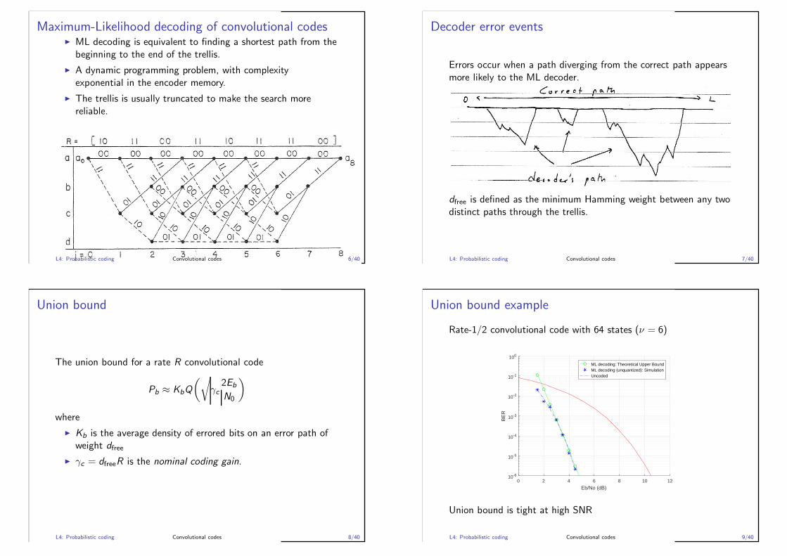
Maximum-Likelihood decoding of convolutional codes◮ ML decoding is equivalent to finding a shortest path from the
beginning to the end of the trellis.
◮ A dynamic programming problem, with complexityexponential in the encoder memory.
◮ The trellis is usually truncated to make the search morereliable.
L4: Probabilistic coding Convolutional codes 6/40
Decoder error events
Errors occur when a path diverging from the correct path appearsmore likely to the ML decoder.
dfree is defined as the minimum Hamming weight between any twodistinct paths through the trellis.
L4: Probabilistic coding Convolutional codes 7/40
Union bound
The union bound for a rate R convolutional code
Pb ≈ KbQ
(√
γc2Eb
N0
)
where
◮ Kb is the average density of errored bits on an error path ofweight dfree
◮ γc = dfreeR is the nominal coding gain.
L4: Probabilistic coding Convolutional codes 8/40
Union bound example
Rate-1/2 convolutional code with 64 states (ν = 6)
0 2 4 6 8 10 12
Eb/No (dB)
10-6
10-5
10-4
10-3
10-2
10-1
100
BE
R
ML decoding: Theoretical Upper BoundML decoding (unquantized): SimulationUncoded
Union bound is tight at high SNR
L4: Probabilistic coding Convolutional codes 9/40

Effective coding gain: γeff
The effective coding gain for a coding system on an AWGNchannel with 2-PAM modulation is defined as
γeff∆=
Eb
N0
∣∣∣∣coded 2-PAM
− Eb
N0
∣∣∣∣uncoded 2-PAM
where the EbNo are the values (in dB) required to achieve a targetBER.
L4: Probabilistic coding Convolutional codes 10/40
Best known convolutional codes
Rate-1/2 binary convolutional codes
ν dfree γc dB Kb γeff (dB)
1 3 1.5 1.8 1 1.82 5 2.5 4.0 1 4.03 6 3 4.8 2 4.64 7 3.5 5.2 4 4.85 8 4 6.0 5 5.66 10 5 7.0 46 5.66 9 4.5 6.5 4 6.17 10 5 7.0 6 6.78 12 6 7.8 10 7.1
◮ ν = log2(no of states)
◮ γeff calculated at Pb = 10−6
L4: Probabilistic coding Convolutional codes 11/40
Best known convolutional codes
Rate-1/3 binary convolutional codes
ν dfree γc dB Kb γeff (dB)
1 5 1.67 2.2 1 2.22 8 2.67 4.3 3 4.03 10 3.33 5.2 6 4.74 12 4 6.0 12 5.35 13 4.33 6.4 1 6.46 15 5 7.0 11 6.37 16 5.33 7.3 1 7.38 18 6 7.8 5 7.4
L4: Probabilistic coding Convolutional codes 12/40
Best known convolutional codes
Rate-1/4 binary convolutional codes
ν dfree γc dB Kb γeff (dB)
1 7 1.75 2.4 1 2.42 10 2.5 4.0 2 3.83 13 3.25 5.1 4 4.74 16 4 6.0 8 5.65 18 4.5 6.5 6 66 20 5 7.0 37 6.07 22 5.5 7.4 2 7.28 24 6 7.8 2 7.6
L4: Probabilistic coding Convolutional codes 13/40
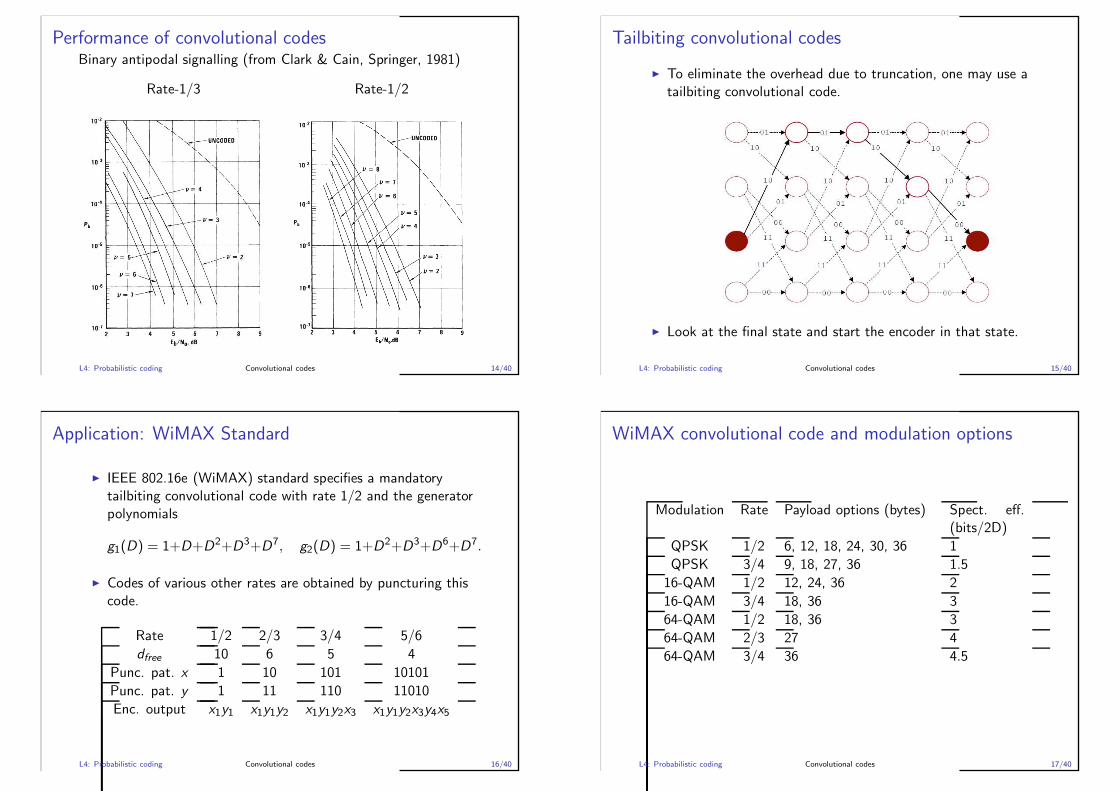
Performance of convolutional codesBinary antipodal signalling (from Clark & Cain, Springer, 1981)
Rate-1/3 Rate-1/2
L4: Probabilistic coding Convolutional codes 14/40
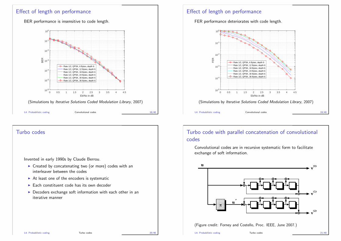
Tailbiting convolutional codes
◮ To eliminate the overhead due to truncation, one may use atailbiting convolutional code.
◮ Look at the final state and start the encoder in that state.
L4: Probabilistic coding Convolutional codes 15/40
Application: WiMAX Standard
◮ IEEE 802.16e (WiMAX) standard specifies a mandatorytailbiting convolutional code with rate 1/2 and the generatorpolynomials
g1(D) = 1+D+D2+D3+D7, g2(D) = 1+D2+D3+D6+D7.
◮ Codes of various other rates are obtained by puncturing thiscode.
Rate 1/2 2/3 3/4 5/6
dfree 10 6 5 4
Punc. pat. x 1 10 101 10101
Punc. pat. y 1 11 110 11010
Enc. output x1y1 x1y1y2 x1y1y2x3 x1y1y2x3y4x5
L4: Probabilistic coding Convolutional codes 16/40
WiMAX convolutional code and modulation options
Modulation Rate Payload options (bytes) Spect. eff.(bits/2D)
QPSK 1/2 6, 12, 18, 24, 30, 36 1
QPSK 3/4 9, 18, 27, 36 1.5
16-QAM 1/2 12, 24, 36 2
16-QAM 3/4 18, 36 3
64-QAM 1/2 18, 36 3
64-QAM 2/3 27 4
64-QAM 3/4 36 4.5
L4: Probabilistic coding Convolutional codes 17/40
Effect of length on performance
BER performance is insensitive to code length.
0 0.5 1 1.5 2 2.5 3 3.5 4 4.5
Eb/No in dB
10-6
10-5
10-4
10-3
10-2
10-1
100
BE
R
Rate 1/2, QPSK, 6 Bytes, depth 6Rate 1/2, QPSK, 12 Bytes, depth 6Rate 1/2, QPSK, 18 Bytes, depth 6Rate 1/2, QPSK, 24 Bytes, depth 6Rate 1/2, QPSK, 30 Bytes, depth 6Rate 1/2, QPSK, 36 Bytes, depth 6
(Simulations by Iterative Solutions Coded Modulation Library, 2007)
L4: Probabilistic coding Convolutional codes 18/40
Effect of length on performance
FER performance deteriorates with code length.
0 0.5 1 1.5 2 2.5 3 3.5 4 4.5
Eb/No in dB
10-5
10-4
10-3
10-2
10-1
100
FE
R
Rate 1/2, QPSK, 6 Bytes, depth 6Rate 1/2, QPSK, 12 Bytes, depth 6Rate 1/2, QPSK, 18 Bytes, depth 6Rate 1/2, QPSK, 24 Bytes, depth 6Rate 1/2, QPSK, 30 Bytes, depth 6Rate 1/2, QPSK, 36 Bytes, depth 6
(Simulations by Iterative Solutions Coded Modulation Library, 2007)
L4: Probabilistic coding Convolutional codes 19/40
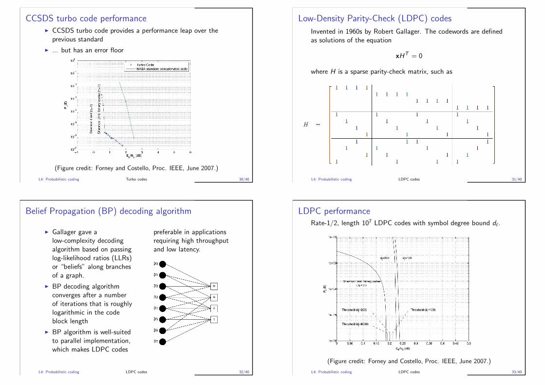
Turbo codes
Invented in early 1990s by Claude Berrou.
◮ Created by concatenating two (or more) codes with aninterleaver between the codes
◮ At least one of the encoders is systematic
◮ Each constituent code has its own decoder
◮ Decoders exchange soft information with each other in aniterative manner
L4: Probabilistic coding Turbo codes 20/40
Turbo code with parallel concatenation of convolutional
codes
Convolutional codes are in recursive systematic form to facilitateexchange of soft information.
(Figure credit: Forney and Costello, Proc. IEEE, June 2007.)
L4: Probabilistic coding Turbo codes 21/40

Turbo decoder
Turbo decoder for parallel concatenated turbo code uses twoseparate decoders that exchange soft information.
(Figure credit: Forney and Costello, Proc. IEEE, June 2007.)
L4: Probabilistic coding Turbo codes 22/40
Turbo code performance
Turbo codes improved the state-of-the-art by a wide margin!
(Figure credit: Forney and Costello, Proc. IEEE, June 2007.)
L4: Probabilistic coding Turbo codes 23/40
WiMAX Convolutional Turbo Codes (CTC)
IEEE 802.16e (WiMAX) specifies a CTC with constituent codes ofrate 2/3 (“duobinary”).
L4: Probabilistic coding Turbo codes 24/40
WiMAX CTC Adaptive Modulation and Coding (AMC)
WiMAX CTC offers a number of AMC options with variouspayload sizes.
Rate Modulation Spect. Eff. Payload options(b/2D) (bytes)
1/2 QPSK 1 12, 24, 36, 48, 60, 72,96, 108, 120
3/4 QPSK 1.5 9, 18, 27, 36, 45, 54
1/2 16-QAM 2 24, 48, 72, 96, 120
3/4 16-QAM 3 18, 36, 54
1/2 64-QAM 3 36, 72, 108
2/3 64-QAM 4 36, 72
3/4 64-QAM 4.5 36, 72
5/6 64-QAM 5 36, 72
L4: Probabilistic coding Turbo codes 25/40
WiMAX CTC performance: QPSK, Rate 1/2The figure shows the WiMAX CTC performance at half-rate withQPSK (4-QAM) modulation with payload ranging from 6 to 120bytes. (Shannon limit is EbNo = 0.188 dB.)
0 0.5 1 1.5 2 2.5 3 3.5 4 4.5
Eb/No in dB
10-7
10-6
10-5
10-4
10-3
10-2
10-1
100B
ER
(Simulations by Iterative Solutions Coded Modulation Library, 2007)L4: Probabilistic coding Turbo codes 26/40
WiMAX CTC performance vs spectral efficiencyThe figure shows the WiMAX CTC performance as the spectralefficiency ranges over 1, 1.5, 2, 3, 4, 4.5, 5 b/2D.
0 2 4 6 8 10 12
Eb/No in dB
10-6
10-5
10-4
10-3
10-2
10-1
100
BE
R
(120,60) QPSK AWGN(72,54) QPSK AWGN(120,60) 16-QAM AWGN(72,54) 16-QAM AWGN(108,54) 64-QAM AWGN(72,48) 64-QAM AWGN(72,54) 64-QAM AWGN(72,60) 64-QAM AWGN
(Simulations by Iterative Solutions Coded Modulation Library, 2007)
L4: Probabilistic coding Turbo codes 27/40
CCSDS (space telemetry) turbo code standard (1999)
L4: Probabilistic coding Turbo codes 28/40
CCSDS turbo code payload and frame size options
CCSDS turbo code supports a wide range of payload and framesizes as shown in the table (all lengths are in bits). Note that thereare 8 bits of termination.
L4: Probabilistic coding Turbo codes 29/40
CCSDS turbo code performance◮ CCSDS turbo code provides a performance leap over the
previous standard
◮ ... but has an error floor
(Figure credit: Forney and Costello, Proc. IEEE, June 2007.)
L4: Probabilistic coding Turbo codes 30/40
Low-Density Parity-Check (LDPC) codes
Invented in 1960s by Robert Gallager. The codewords are definedas solutions of the equation
xHT = 0
where H is a sparse parity-check matrix, such as
L4: Probabilistic coding LDPC codes 31/40
Belief Propagation (BP) decoding algorithm
◮ Gallager gave alow-complexity decodingalgorithm based on passinglog-likelihood ratios (LLRs)or “beliefs” along branchesof a graph.
◮ BP decoding algorithmconverges after a numberof iterations that is roughlylogarithmic in the codeblock length
◮ BP algorithm is well-suitedto parallel implementation,which makes LDPC codes
preferable in applicationsrequiring high throughputand low latency.
L4: Probabilistic coding LDPC codes 32/40
LDPC performanceRate-1/2, length 107 LDPC codes with symbol degree bound dℓ.
(Figure credit: Forney and Costello, Proc. IEEE, June 2007.)
L4: Probabilistic coding LDPC codes 33/40
Application: WiMAX LDPC codes
◮ WiMAX offers a number ofLDPC code alternatives.
◮ These codes may require amaximum of 30 - 100iterations for bestperformance.
◮ LDPC codes are not verysuitable for rate adaptation.
Rate Length
5/6 2304
3/4 2304
2/3 2304
1/2 2304
5/6 576
3/4 576
2/3 576
1/2 576
L4: Probabilistic coding LDPC codes 34/40
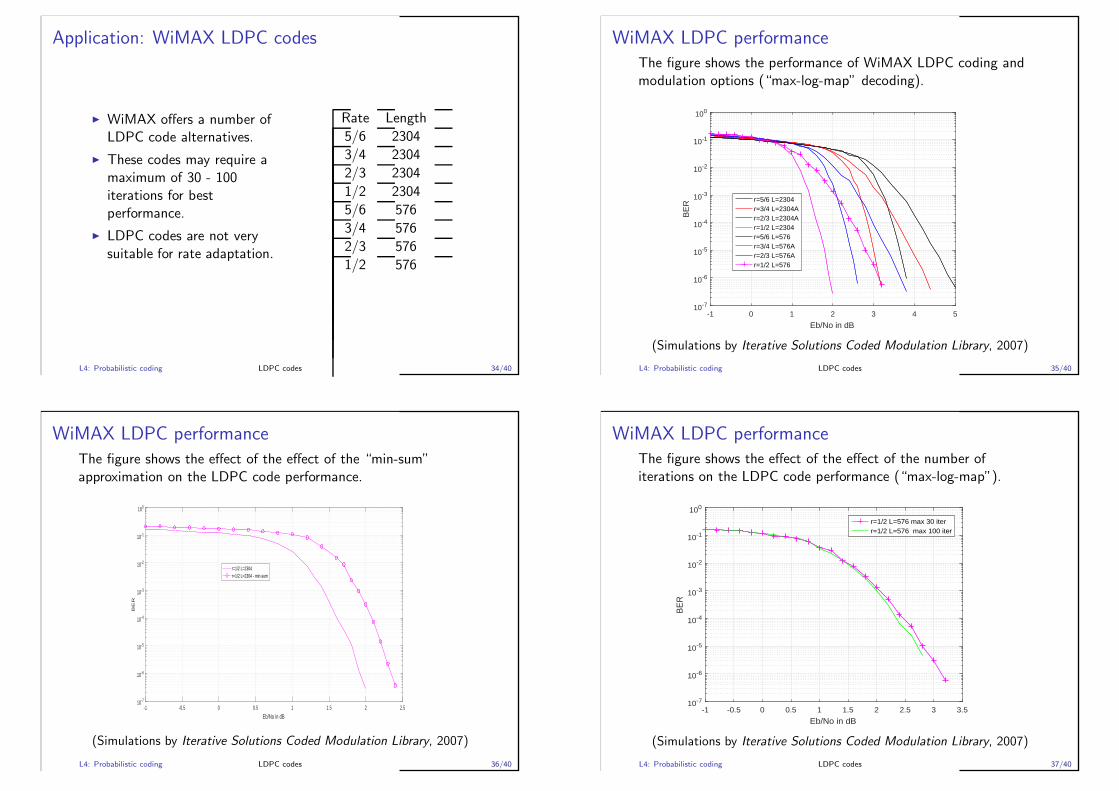
WiMAX LDPC performanceThe figure shows the performance of WiMAX LDPC coding andmodulation options (“max-log-map” decoding).
-1 0 1 2 3 4 5
Eb/No in dB
10-7
10-6
10-5
10-4
10-3
10-2
10-1
100
BE
R r=5/6 L=2304r=3/4 L=2304Ar=2/3 L=2304Ar=1/2 L=2304r=5/6 L=576r=3/4 L=576Ar=2/3 L=576Ar=1/2 L=576
(Simulations by Iterative Solutions Coded Modulation Library, 2007)
L4: Probabilistic coding LDPC codes 35/40
WiMAX LDPC performance
The figure shows the effect of the effect of the “min-sum”approximation on the LDPC code performance.
-1 -0.5 0 0.5 1 1.5 2 2.5
Eb/No in dB
10-7
10-6
10-5
10-4
10-3
10-2
10-1
100
BE
R
r=1/2 L=2304r=1/2 L=2304 - min-sum
(Simulations by Iterative Solutions Coded Modulation Library, 2007)
L4: Probabilistic coding LDPC codes 36/40
WiMAX LDPC performanceThe figure shows the effect of the effect of the number ofiterations on the LDPC code performance (“max-log-map”).
-1 -0.5 0 0.5 1 1.5 2 2.5 3 3.5
Eb/No in dB
10-7
10-6
10-5
10-4
10-3
10-2
10-1
100
BE
R
r=1/2 L=576 max 30 iterr=1/2 L=576 max 100 iter
(Simulations by Iterative Solutions Coded Modulation Library, 2007)
L4: Probabilistic coding LDPC codes 37/40

WiMAX LDPC/CTC performance comparison
The figure shows the relative performance of WiMAX LDPC andCTC codes.
−1 −0.5 0 0.5 1 1.5 2 2.5 3 3.510
−5
10−4
10−3
10−2
10−1
100
Eb/No in dB
FE
R
Turbo (576,288)Turbo (960,480)LDPC,(2304,1162)LDPC, (576,288)
(Simulations by Iterative Solutions Coded Modulation Library, 2007)
L4: Probabilistic coding WiMAX code comparisons 38/40
WiMAX CTC/CC performance comparison
The figure shows the relative performance of WiMAX CTC andWiMAX CC codes.
0 0.5 1 1.5 2 2.5 3 3.5 4 4.5
Eb/No in dB
10-6
10-5
10-4
10-3
10-2
10-1
100
BE
R
CC(12,6), QPSKCC(72,36) QPSKCTC(12,6) QPSKCTC(72,36) QPSK
(Simulations by Iterative Solutions Coded Modulation Library, 2007)
L4: Probabilistic coding WiMAX code comparisons 39/40
Summary
◮ Turbo and LDPC codes solve the coding problem for mostengineering purposes.
◮ Convolutional codes still have a place for very short payloads(up to 100 bits) that need to be protected well (controlchannel).
◮ LDPC codes perform better at long block lengths where highreliability, high throughput is required (optical channels, videochannels).
◮ Turbo codes are superior for applications where packet sizesare moderate and the reliability requirement is not too high(voice applications)
◮ Algebraic codes (RS and BCH in particular) have a role asexternal codes in concatenated schemes.
L4: Probabilistic coding WiMAX code comparisons 40/40
L1: Information theory review
L2: Gaussian channel
L3: Algebraic coding
L4: Probabilistic coding
L5: Channel polarization
L6: Polar coding
L7: Origins of polar coding
L8: Coding for bandlimited channels
L9: Polar codes for selected applications
L5: Channel polarization 1/26
Lecture 5 – Channel polarization
◮ Objective: Explain channel polarization
◮ Topics:
◮ Channel codes as polarizers of information
◮ Low-complexity polarization by channel combining and splitting
◮ The main polarization theorem
◮ Rate of polarization
L5: Channel polarization 2/26
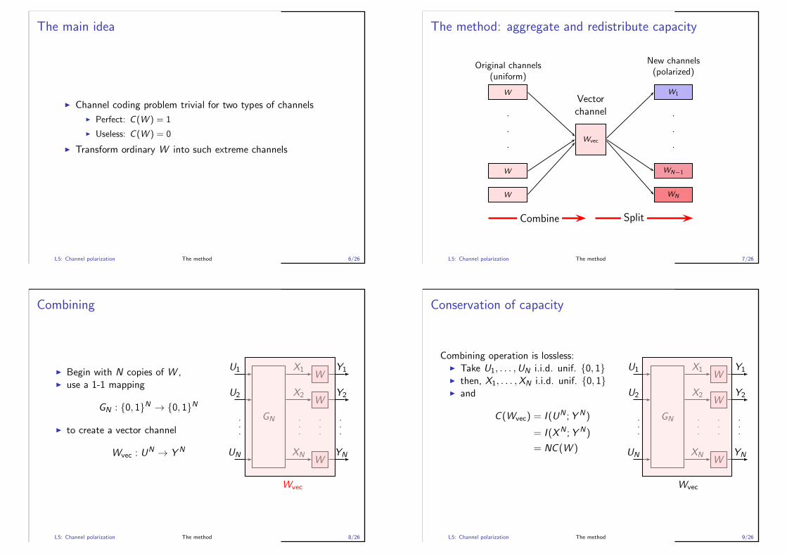
The channel
Let W : X → Y be a binary-input discrete memoryless channel
WX Y
◮ input alphabet: X = {0, 1},◮ output alphabet: Y,◮ transition probabilities:
W (y |x), x ∈ X , y ∈ Y
L5: Channel polarization The setup 3/26
Symmetry assumption
Assume that the channel has “input-output symmetry.”
Examples:
1− ǫ
1− ǫ
ǫ
ǫ
1
0
1
0
BSC(ǫ)
1− ǫ
1− ǫ
ǫ
ǫ
1
0
1
0
?
BEC(ǫ)
L5: Channel polarization The setup 4/26
Capacity
For channels with input-output symmetry, the capacity is given by
C (W )∆= I (X ;Y ), with X ∼ unif. {0, 1}
Use base-2 logarithms:
0 ≤ C (W ) ≤ 1
L5: Channel polarization The setup 5/26
The main idea
◮ Channel coding problem trivial for two types of channels
◮ Perfect: C (W ) = 1
◮ Useless: C (W ) = 0
◮ Transform ordinary W into such extreme channels
L5: Channel polarization The method 6/26
The method: aggregate and redistribute capacity
W
W
b
b
b
W
Original channels(uniform)
Wvec
Vectorchannel
Combine
WN
WN−1
b
b
b
W1
Split
New channels(polarized)
L5: Channel polarization The method 7/26
Combining
◮ Begin with N copies of W ,◮ use a 1-1 mapping
GN : {0, 1}N → {0, 1}N
◮ to create a vector channel
Wvec : UN → Y N
W
W
WXN
X2
X1
YN
Y2
Y1
GN
UN
U2
U1
Wvec
L5: Channel polarization The method 8/26
Conservation of capacity
Combining operation is lossless:◮ Take U1, . . . ,UN i.i.d. unif. {0, 1}◮ then, X1, . . . ,XN i.i.d. unif. {0, 1}◮ and
C (Wvec) = I (UN ;Y N)
= I (XN ;Y N)
= NC (W )
W
W
W
GN
XN
X2
X1
YN
Y2
Y1
UN
U2
U1
Wvec
L5: Channel polarization The method 9/26
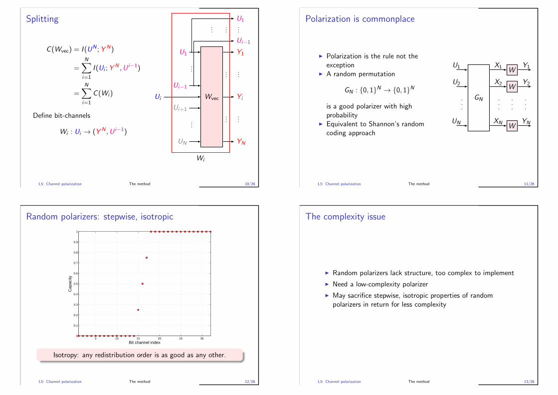
Splitting
C (Wvec) = I (UN ;Y N)
=
N∑
i=1
I (Ui ;YN ,U i−1)
=N∑
i=1
C (Wi )
Define bit-channels
Wi : Ui → (Y N ,U i−1)
Wvec
UN
Ui+1
Ui
Ui−1
U1
U1
Ui−1
YN
Yi
Y1
Wi
L5: Channel polarization The method 10/26
Polarization is commonplace
◮ Polarization is the rule not theexception
◮ A random permutation
GN : {0, 1}N → {0, 1}N
is a good polarizer with highprobability
◮ Equivalent to Shannon’s randomcoding approach
W
W
W
GN
XN
X2
X1
YN
Y2
Y1
UN
U2
U1
L5: Channel polarization The method 11/26
Random polarizers: stepwise, isotropic
5 10 15 20 25 300
0.1
0.2
0.3
0.4
0.5
0.6
0.7
0.8
0.9
1
Bit channel index
Cap
acity
Isotropy: any redistribution order is as good as any other.
L5: Channel polarization The method 12/26
The complexity issue
◮ Random polarizers lack structure, too complex to implement
◮ Need a low-complexity polarizer
◮ May sacrifice stepwise, isotropic properties of randompolarizers in return for less complexity
L5: Channel polarization The method 13/26
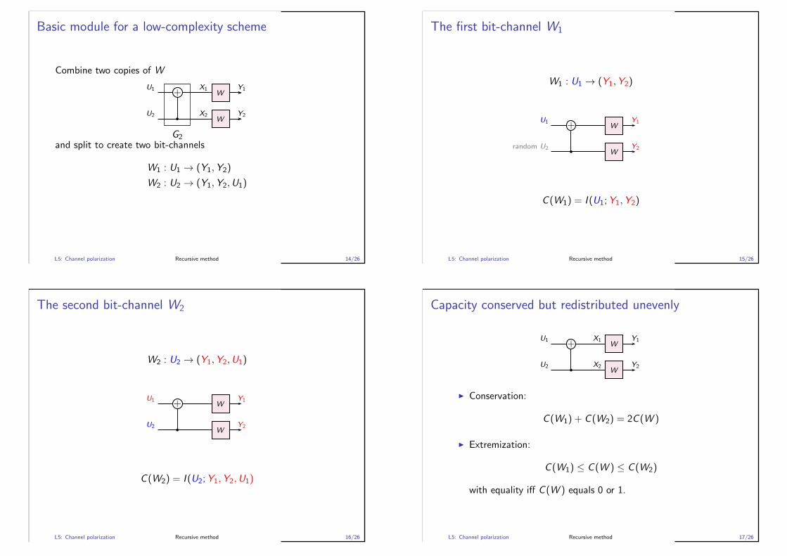
Basic module for a low-complexity scheme
Combine two copies of W
+
U2
U1
G2
W
W
Y2
Y1
X2
X1
and split to create two bit-channels
W1 : U1 → (Y1,Y2)
W2 : U2 → (Y1,Y2,U1)
L5: Channel polarization Recursive method 14/26
The first bit-channel W1
W1 : U1 → (Y1,Y2)
+
random U2
U1
W
W
Y2
Y1
C (W1) = I (U1;Y1,Y2)
L5: Channel polarization Recursive method 15/26
The second bit-channel W2
W2 : U2 → (Y1,Y2,U1)
+
U2
U1
W
W
Y2
Y1
C (W2) = I (U2;Y1,Y2,U1)
L5: Channel polarization Recursive method 16/26
Capacity conserved but redistributed unevenly
+
U2
U1
W
W
Y2
Y1
X2
X1
◮ Conservation:
C (W1) + C (W2) = 2C (W )
◮ Extremization:
C (W1) ≤ C (W ) ≤ C (W2)
with equality iff C (W ) equals 0 or 1.
L5: Channel polarization Recursive method 17/26
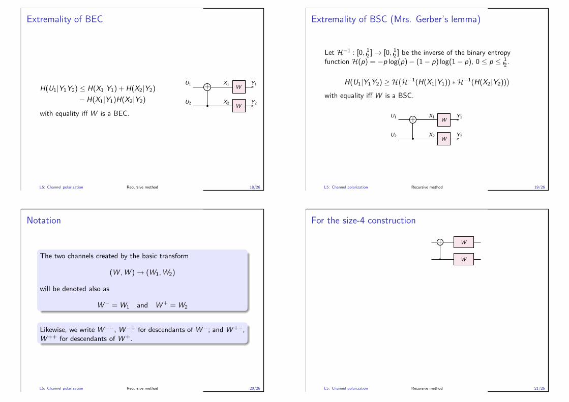
Extremality of BEC
H(U1|Y1Y2) ≤ H(X1|Y1) + H(X2|Y2)
− H(X1|Y1)H(X2|Y2)
with equality iff W is a BEC.
+
U2
U1
W
W
Y2
Y1
X2
X1
L5: Channel polarization Recursive method 18/26
Extremality of BSC (Mrs. Gerber’s lemma)
Let H−1 : [0, 12 ] → [0, 12 ] be the inverse of the binary entropyfunction H(p) = −p log(p)− (1− p) log(1− p), 0 ≤ p ≤ 1
2 .
H(U1|Y1Y2) ≥ H(H−1(H(X1|Y1)) ∗ H−1(H(X2|Y2))
)
with equality iff W is a BSC.
+
U2
U1
W
W
Y2
Y1
X2
X1
L5: Channel polarization Recursive method 19/26
Notation
The two channels created by the basic transform
(W ,W ) → (W1,W2)
will be denoted also as
W− = W1 and W+ = W2
Likewise, we write W−−, W−+ for descendants of W−; and W+−,W++ for descendants of W+.
L5: Channel polarization Recursive method 20/26
For the size-4 construction
+
W
W
L5: Channel polarization Recursive method 21/26
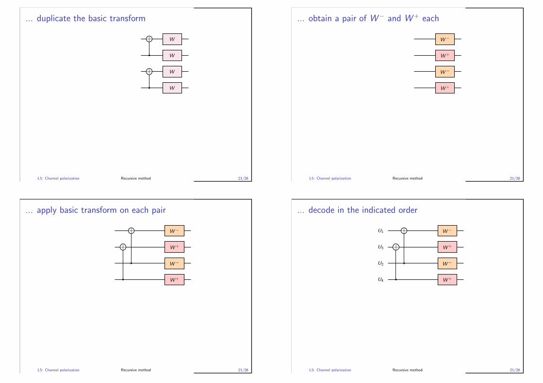
... duplicate the basic transform
+
+
W
W
W
W
L5: Channel polarization Recursive method 21/26
... obtain a pair of W− and W+ each
W+
W+
W−
W−
L5: Channel polarization Recursive method 21/26
... apply basic transform on each pair
+
+
W+
W+
W−
W−
L5: Channel polarization Recursive method 21/26
... decode in the indicated order
+
+
W+
W+
W−
W−
U4
U2
U3
U1
L5: Channel polarization Recursive method 21/26
... obtain the four new bit-channels
W++
W−+
W+−
W−−
U4
U2
U3
U1
L5: Channel polarization Recursive method 21/26
Overall size-4 construction
+
+
+
+
W
W
W
W
U4
U2
U3
U1
Y4
Y2
Y3
Y1
X4
X2
X3
X1
L5: Channel polarization Recursive method 21/26
“Rewire” for standard-form size-4 construction
+
+
+
+
W
W
W
W
U4
U3
U2
U1
Y4
Y3
Y2
Y1
X4
X3
X2
X1
L5: Channel polarization Recursive method 21/26
Size 8 construction
+
+
+
+
+
+
+
+
+
+
+
+
W
W
W
W
W
W
W
W
Y8
Y7
Y6
Y5
Y4
Y3
Y2
Y1
U8
U7
U6
U5
U4
U3
U2
U1
X8
X7
X6
X5
X4
X3
X2
X1
L5: Channel polarization Recursive method 22/26
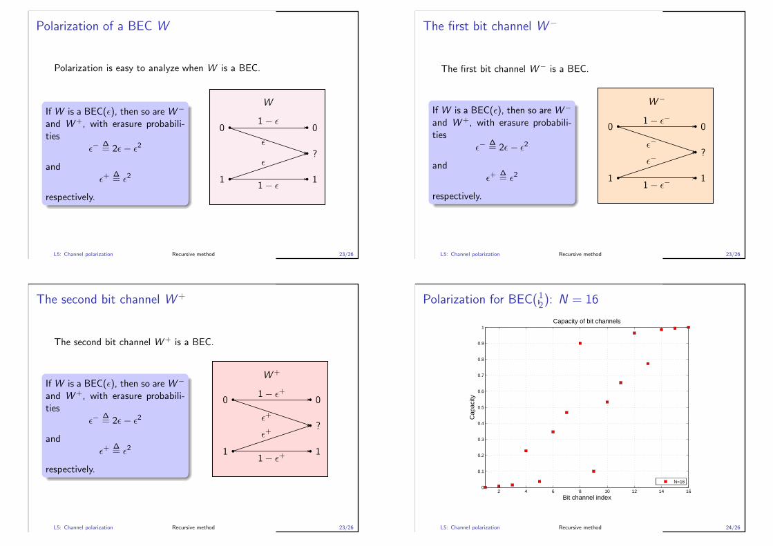
Polarization of a BEC W
Polarization is easy to analyze when W is a BEC.
If W is a BEC(ǫ), then so are W−
and W+, with erasure probabili-ties
ǫ−∆= 2ǫ− ǫ2
andǫ+
∆= ǫ2
respectively.1− ǫ
1− ǫ
ǫ
ǫ
1
0
1
0
?
W
L5: Channel polarization Recursive method 23/26
The first bit channel W−
The first bit channel W− is a BEC.
If W is a BEC(ǫ), then so are W−
and W+, with erasure probabili-ties
ǫ−∆= 2ǫ− ǫ2
andǫ+
∆= ǫ2
respectively.1− ǫ−
1− ǫ−
ǫ−ǫ−
1
0
1
0
?
W−
L5: Channel polarization Recursive method 23/26
The second bit channel W+
The second bit channel W+ is a BEC.
If W is a BEC(ǫ), then so are W−
and W+, with erasure probabili-ties
ǫ−∆= 2ǫ− ǫ2
andǫ+
∆= ǫ2
respectively.1− ǫ+
1− ǫ+
ǫ+
ǫ+
1
0
1
0
?
W+
L5: Channel polarization Recursive method 23/26
Polarization for BEC(12): N = 16
2 4 6 8 10 12 14 160
0.1
0.2
0.3
0.4
0.5
0.6
0.7
0.8
0.9
1
Bit channel index
Cap
acity
Capacity of bit channels
N=16
L5: Channel polarization Recursive method 24/26
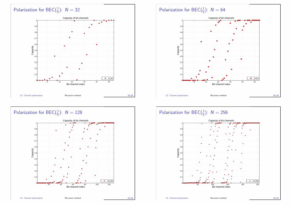
Polarization for BEC(12): N = 32
5 10 15 20 25 300
0.1
0.2
0.3
0.4
0.5
0.6
0.7
0.8
0.9
1
Bit channel index
Cap
acity
Capacity of bit channels
N=32
L5: Channel polarization Recursive method 24/26
Polarization for BEC(12): N = 64
10 20 30 40 50 600
0.1
0.2
0.3
0.4
0.5
0.6
0.7
0.8
0.9
1
Bit channel index
Cap
acity
Capacity of bit channels
N=64
L5: Channel polarization Recursive method 24/26
Polarization for BEC(12): N = 128
20 40 60 80 100 1200
0.1
0.2
0.3
0.4
0.5
0.6
0.7
0.8
0.9
1
Bit channel index
Cap
acity
Capacity of bit channels
N=128
L5: Channel polarization Recursive method 24/26
Polarization for BEC(12): N = 256
50 100 150 200 2500
0.1
0.2
0.3
0.4
0.5
0.6
0.7
0.8
0.9
1
Bit channel index
Cap
acity
Capacity of bit channels
N=256
L5: Channel polarization Recursive method 24/26

Polarization for BEC(12): N = 512
50 100 150 200 250 300 350 400 450 5000
0.1
0.2
0.3
0.4
0.5
0.6
0.7
0.8
0.9
1
Bit channel index
Cap
acity
Capacity of bit channels
N=512
L5: Channel polarization Recursive method 24/26
Polarization for BEC(12): N = 1024
100 200 300 400 500 600 700 800 900 10000
0.1
0.2
0.3
0.4
0.5
0.6
0.7
0.8
0.9
1
Bit channel index
Cap
acity
Capacity of bit channels
N=1024
L5: Channel polarization Recursive method 24/26
Polarization martingale
0
1
1 22 3333 44444444 5555555555555555 66666666666666666666666666666666 7777777777777777777777777777777777777777777777777777777777777777 88888888888888888888888888888888888888888888888888888888888888888888888888888888888888888888888888888888888888888888888888888888
C(W )
C(W2)
C(W1)
C(W++)
C(W−+)
C(W+−)
C(W−−)
L5: Channel polarization Recursive method 25/26
Theorem (Polarization, A. 2007)
The bit-channel capacities {C (Wi )} polarize: for anyδ ∈ (0, 1), as the construction size N grows
[no. channels with C (Wi) > 1− δ
N
]
−→ C (W )
and[no. channels with C (Wi) < δ
N
]
−→ 1− C (W )
Theorem (Rate of polarization, A. and Telatar (2008))
Above theorem holds with δ ≈ 2−√N .
0
δ
1− δ
1
L5: Channel polarization Recursive method 26/26
L1: Information theory review
L2: Gaussian channel
L3: Algebraic coding
L4: Probabilistic coding
L5: Channel polarization
L6: Polar coding
L7: Origins of polar coding
L8: Coding for bandlimited channels
L9: Polar codes for selected applications
L6: Polar coding 1/45
Lecture 6 – Polar coding
◮ Objective: Introduce polar coding
◮ Topics
◮ Code construction
◮ Encoding
◮ Decoding
◮ Performance
L6: Polar coding 2/45
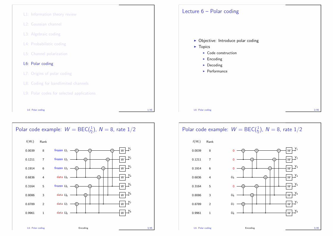
Polar code example: W = BEC(12), N = 8, rate 1/2
I (Wi )
0.0039
0.1211
0.1914
0.6836
0.3164
0.8086
0.8789
0.9961
Rank
8
7
6
4
5
3
2
1
+
+
+
+
+
+
+
+
+
+
+
+
W
W
W
W
W
W
W
W
Y8
Y7
Y6
Y5
Y4
Y3
Y2
Y1
U8
U7
U6
U5
U4
U3
U2
U1
data
data
data
frozen
data
frozen
frozen
frozen
L6: Polar coding Encoding 3/45
Polar code example: W = BEC(12), N = 8, rate 1/2
I (Wi )
0.0039
0.1211
0.1914
0.6836
0.3164
0.8086
0.8789
0.9961
Rank
8
7
6
4
5
3
2
1
+
+
+
+
+
+
+
+
+
+
+
+
W
W
W
W
W
W
W
W
Y8
Y7
Y6
Y5
Y4
Y3
Y2
Y1
U8
U7
U6
0
U4
0
0
0
L6: Polar coding Encoding 3/45
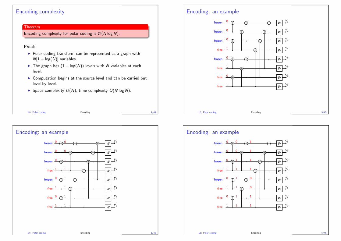
Encoding complexity
Theorem
Encoding complexity for polar coding is O(N logN).
Proof:
◮ Polar coding transform can be represented as a graph withN[1 + log(N)] variables.
◮ The graph has (1 + log(N)) levels with N variables at eachlevel.
◮ Computation begins at the source level and can be carried outlevel by level.
◮ Space complexity O(N), time complexity O(N logN).
L6: Polar coding Encoding 4/45
Encoding: an example
+
+
+
+
+
+
+
+
+
+
+
+
W
W
W
W
W
W
W
W
Y8
Y7
Y6
Y5
Y4
Y3
Y2
Y1
1
0
1
0
1
0
0
0
free
free
free
frozen
free
frozen
frozen
frozen
L6: Polar coding Encoding 5/45
Encoding: an example
+
+
+
+
+
+
+
+
+
+
+
+
W
W
W
W
W
W
W
W
Y8
Y7
Y6
Y5
Y4
Y3
Y2
Y1
1
0
1
0
1
0
0
0
1
1
1
1
1
1
0
0
free
free
free
frozen
free
frozen
frozen
frozen
L6: Polar coding Encoding 5/45
Encoding: an example
+
+
+
+
+
+
+
+
+
+
+
+
W
W
W
W
W
W
W
W
Y8
Y7
Y6
Y5
Y4
Y3
Y2
Y1
1
0
1
0
1
0
0
0
1
1
1
1
1
1
0
0
1
1
0
0
1
1
1
1
free
free
free
frozen
free
frozen
frozen
frozen
L6: Polar coding Encoding 5/45
Encoding: an example
+
+
+
+
+
+
+
+
+
+
+
+
W
W
W
W
W
W
W
W
Y8
Y7
Y6
Y5
Y4
Y3
Y2
Y1
1
0
1
0
1
0
0
0
1
1
1
1
1
1
0
0
1
1
0
0
1
1
1
1
1
1
0
0
0
0
1
1
free
free
free
frozen
free
frozen
frozen
frozen
L6: Polar coding Encoding 5/45
Successive Cancellation Decoding (SCD)
Theorem
The complexity of successive cancellation decoding for polar codesis O(N logN).
Proof: Given below.
L6: Polar coding Decoding 6/45
SCD: Exploit the x = |a|a+ b| structure
+
+
+
+
+
+
+
+
+
+
+
+
W
W
W
W
W
W
W
W
y8
y7
y6
y5
y4
y3
y2
y1
u8
u7
u6
u5
u4
u3
u2
u1
x8
x7
x6
x5
x4
x3
x2
x1
a4
a3
a2
a1
b4
b3
b2
b1
L6: Polar coding Decoding 7/45
First phase: treat a as noise, decode (u1, u2, u3, u4)
+
+
+
+
+
+
+
+
W
W
W
W
W
W
W
W
u4
u3
u2
u1
x8
x7
x6
x5
x4
x3
x2
x1
y8
y7
y6
y5
y4
y3
y2
y1
noise a4
noise a3
noise a2
noise a1
b4
b3
b2
b1
L6: Polar coding Decoding 8/45

End of first phase
+
+
+
+
+
+
+
+
+
+
+
+
W
W
W
W
W
W
W
W
y8
y7
y6
y5
y4
y3
y2
y1
u8
u7
u6
u5
u4
u3
u2
u1
x8
x7
x6
x5
x4
x3
x2
x1
a4
a3
a2
a1
b4
b3
b2
b1
L6: Polar coding Decoding 9/45
Second phase: Treat b as known, decode (u5, u6, u7, u8)
+
+
+
+
+
+
+
+
W
W
W
W
W
W
W
W
u8
u7
u6
u5
y8
y7
y6
y5
y4
y3
y2
y1
a4
a3
a2
a1
known b4
known b3
known b2
known b1
L6: Polar coding Decoding 10/45
First phase in detail
+
+
+
+
+
+
+
+
W
W
W
W
W
W
W
W
u4
u3
u2
u1
x8
x7
x6
x5
x4
x3
x2
x1
y8
y7
y6
y5
y4
y3
y2
y1
noise a4
noise a3
noise a2
noise a1
b4
b3
b2
b1
L6: Polar coding Decoding 11/45
Equivalent channel model
+
+
+
+
W
W
W
W
W
W
W
W
x8
x7
x6
x5
x4
x3
x2
x1
y8
y7
y6
y5
y4
y3
y2
y1
noise a4
noise a3
noise a2
noise a1
b4
b3
b2
b1
L6: Polar coding Decoding 12/45
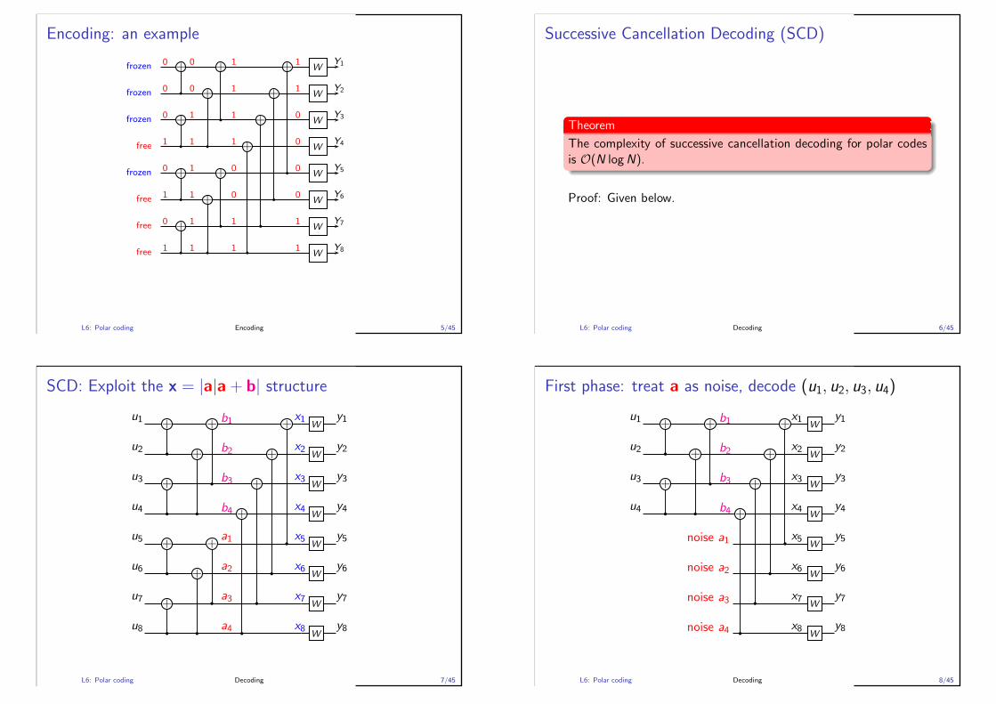
First copy of W−
+
+
+
+
W
W
W
W
W
W
W
W
W
W
x8
x7
x6
x5
x4
x3
x2
x1
y8
y7
y6
y5
y4
y3
y2
y1
noise a4
noise a3
noise a2
noise a1
b4
b3
b2
b1
L6: Polar coding Decoding 13/45
Second copy of W−
+
+
+
+
W
W
W
W
W
W
W
W
W
W
x8
x7
x6
x5
x4
x3
x2
x1
y8
y7
y6
y5
y4
y3
y2
y1
noise a4
noise a3
noise a2
noise a1
b4
b3
b2
b1
L6: Polar coding Decoding 14/45
Third copy of W−
+
+
+
+
W
W
W
W
W
W
W
W
W
W
x8
x7
x6
x5
x4
x3
x2
x1
y8
y7
y6
y5
y4
y3
y2
y1
noise a4
noise a3
noise a2
noise a1
b4
b3
b2
b1
L6: Polar coding Decoding 15/45
Fourth copy of W−
+
+
+
+
W
W
W
W
W
W
W
W
W
W
x8
x7
x6
x5
x4
x3
x2
x1
y8
y7
y6
y5
y4
y3
y2
y1
noise a4
noise a3
noise a2
noise a1
b4
b3
b2
b1
L6: Polar coding Decoding 16/45
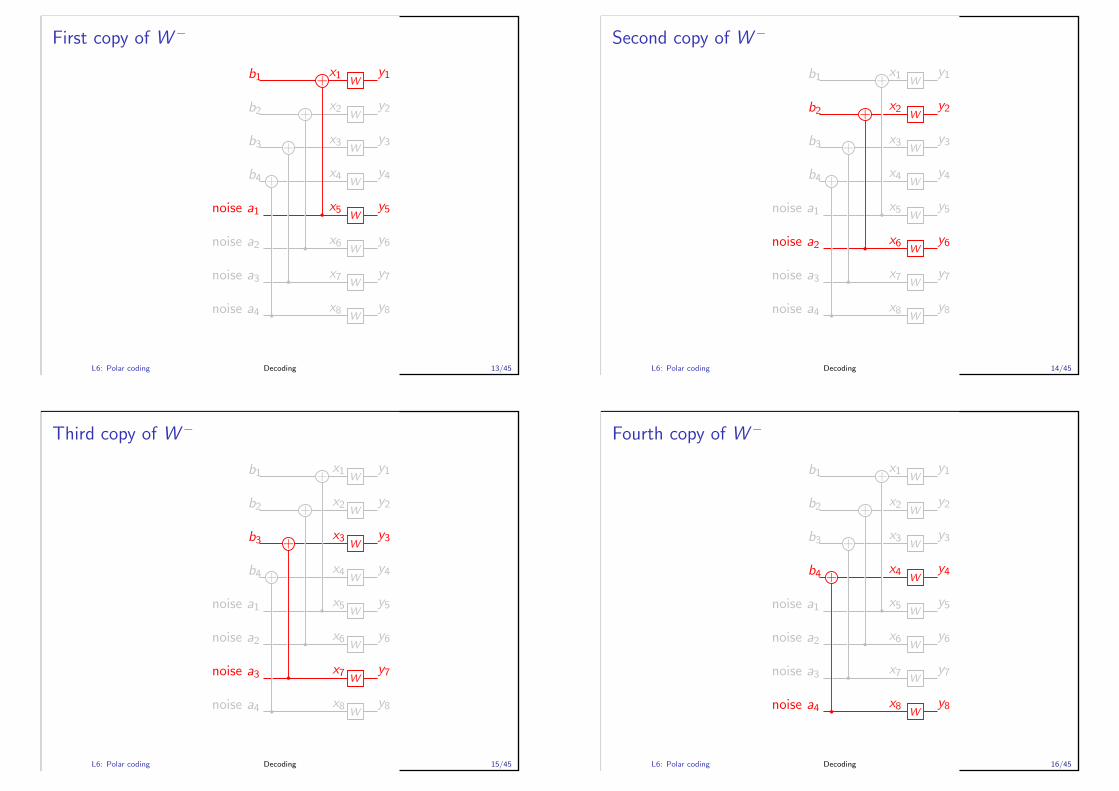
Decoding on W−
+
+
+
+
W−
W−
W−
W−
u4
u3
u2
u1
(y4, y8)
(y3, y7)
(y2, y6)
(y1, y5)
b4
b3
b2
b1
L6: Polar coding Decoding 17/45
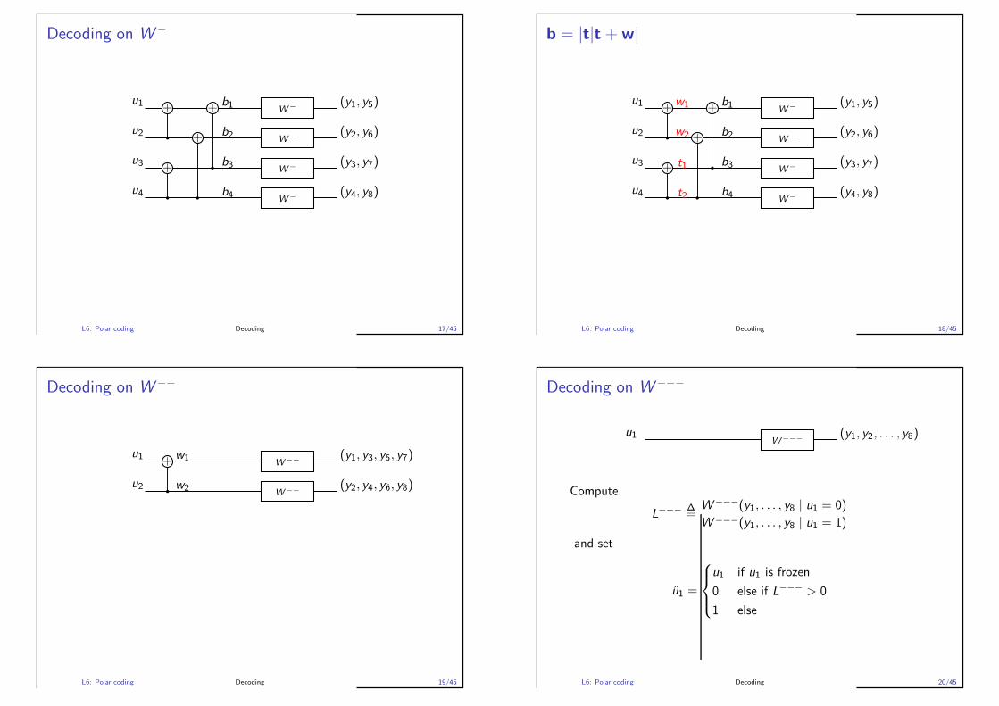
b = |t|t + w|
+
+
+
+
W−
W−
W−
W−
u4
u3
u2
u1
(y4, y8)
(y3, y7)
(y2, y6)
(y1, y5)
b4
b3
b2
b1
t2
t1
w2
w1
L6: Polar coding Decoding 18/45
Decoding on W−−
+
W−−
W−−
u2
u1
(y2, y4, y6, y8)
(y1, y3, y5, y7)
w2
w1
L6: Polar coding Decoding 19/45
Decoding on W−−−
W−−−u1 (y1, y2, . . . , y8)
Compute
L−−− ∆=
W−−−(y1, . . . , y8 | u1 = 0)
W−−−(y1, . . . , y8 | u1 = 1)
and set
u1 =
u1 if u1 is frozen
0 else if L−−− > 0
1 else
L6: Polar coding Decoding 20/45
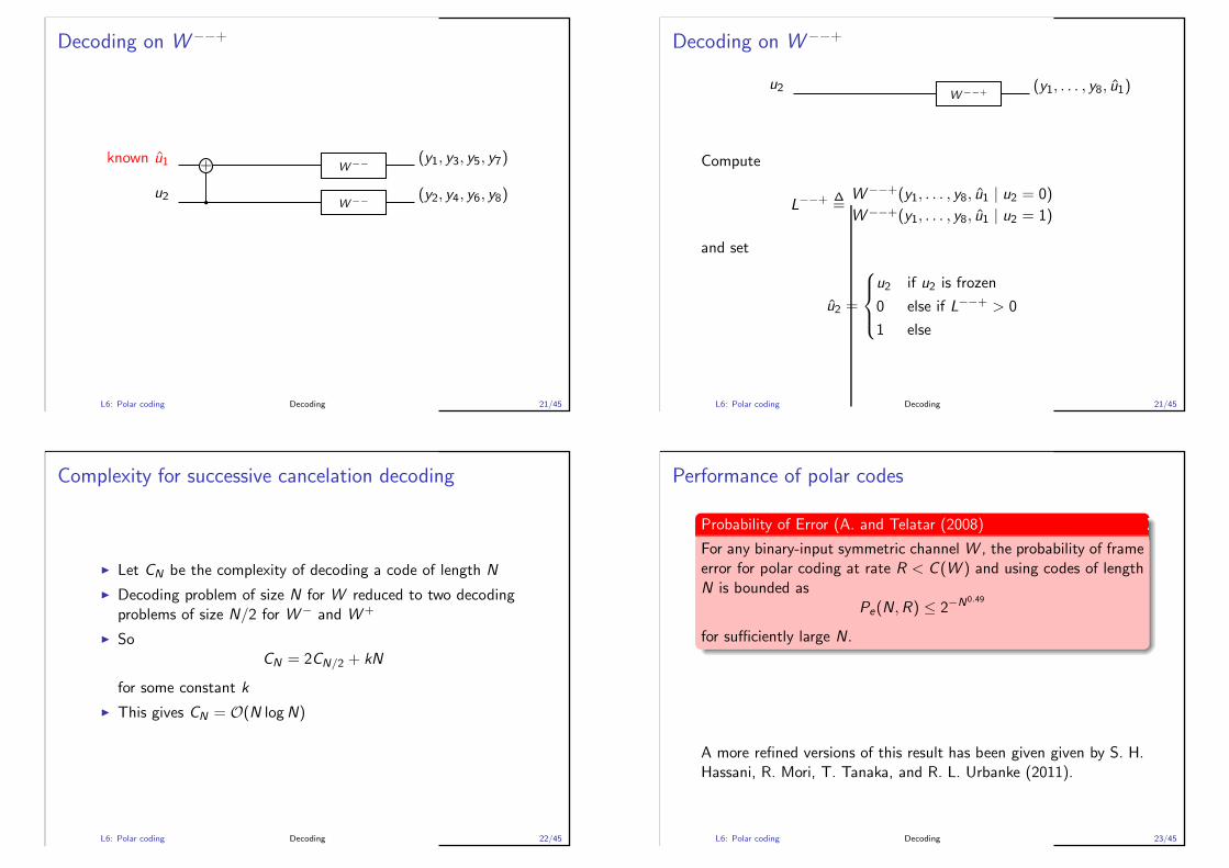
Decoding on W−−+
+
W−−
W−−
u2
known u1
(y2, y4, y6, y8)
(y1, y3, y5, y7)
L6: Polar coding Decoding 21/45
Decoding on W−−+
W−−+u2 (y1, . . . , y8, u1)
Compute
L−−+ ∆=
W−−+(y1, . . . , y8, u1 | u2 = 0)
W−−+(y1, . . . , y8, u1 | u2 = 1)
and set
u2 =
u2 if u2 is frozen
0 else if L−−+ > 0
1 else
L6: Polar coding Decoding 21/45
Complexity for successive cancelation decoding
◮ Let CN be the complexity of decoding a code of length N
◮ Decoding problem of size N for W reduced to two decodingproblems of size N/2 for W− and W+
◮ SoCN = 2CN/2 + kN
for some constant k
◮ This gives CN = O(N logN)
L6: Polar coding Decoding 22/45
Performance of polar codes
Probability of Error (A. and Telatar (2008)
For any binary-input symmetric channel W , the probability of frameerror for polar coding at rate R < C (W ) and using codes of lengthN is bounded as
Pe(N,R) ≤ 2−N0.49
for sufficiently large N.
A more refined versions of this result has been given given by S. H.Hassani, R. Mori, T. Tanaka, and R. L. Urbanke (2011).
L6: Polar coding Decoding 23/45

Construction complexity
Construction Complexity
Polar codes can be constructed in time O(Npoly(log(N))).
This result has been developed in a sequence of papers by
◮ R. Mori and T. Tanaka (2009)
◮ I. Tal and A. Vardy (2011)
◮ R. Pedarsani, S. H. Hassani, I. Tal, and E. Telatar (2011)
L6: Polar coding Construction 24/45
Gaussian approximation
◮ Trifonov (2011) introduced a Gaussian approximationtechnique for constructing polar codes
◮ Dai et al. (2015) studied various refinements of Gaussianapproximation for polar code construction
◮ These methods work extremely well although a satisfactoryexplanation of why they work is still missing
L6: Polar coding Construction 25/45
Example of Gaussian approximation
Polar code construction and performance estimation by Gaussianapproximation
0 1 2 3 4 5 6 7 8
Es/N
0 (dB)
10-6
10-5
10-4
10-3
10-2
10-1
100
FE
R
Polar(65536,61440,8) - BPSKUltimate Shannon limitBPSK Shannon limitThreshold SNR at target FERGaussian approximation
Shannon BPSK limit
Shannon limit
Gap to ultimate capacity = 3.42Gap to BPSK capacity = 1.06
L6: Polar coding Construction 26/45
Polar coding summary
Summary
Given W , N = 2n, and R < I (W ), a polar code can be constructedsuch that it has
◮ construction complexity O(Npoly(log(N))),◮ encoding complexity ≈ N logN,◮ successive-cancellation decoding complexity ≈ N logN,
◮ frame error probability Pe(N,R) = o(
2−√N+o(
√N))
.
L6: Polar coding Construction 27/45
Performance improvement for polar codes
◮ Concatenation to improve minimum distance
◮ List decoding to improve SC decoder performance
L6: Polar coding Performance 28/45
Concatenation
Method Ref
Block turbo coding with polar constituents AKMOP (2009)Generalized concatenated coding with polar inner AM (2009)Reed-Solomon outer, polar inner BJE (2010)Polar outer, block inner SH (2010)Polar outer, LDPC inner EP (ISIT’2011)
AKMOP: A., Kim, Markarian, Ozgur, PoyrazGCC: A., MarkarianBJE: Bakshi, Jaggi, and EffrosSH: Seidl and HuberEP: Eslami and Pishro-Nik
L6: Polar coding Performance 29/45
Overview of decoders for polar codes◮ Successive cancellation decoding: A depth-first search method
with complexity roughly N logN
◮ Sufficient to prove that polar codes achieve capacity
◮ Equivalent to an earlier algorithm by Schnabl and Bossert(1995) for RM codes
◮ Simple but not powerful enough to challenge LDPC and turbocodes in short to moderate lengths
◮ List decoding: A breadth-first search algorithm with limitedbranching (known as “beam search” in AI).
◮ First proposed by Tal and Vardy (2011) for polar codes.
◮ List decoding was used earlier by Dumer and Shabunov (2006)for RM codes
◮ Complexity grows as O(LN logN) for a list size L. Buthardware implementation becomes problematic as L grows dueto sorting and memory management.
◮ Sphere-decoding (“British Museum” search with branch andbound, starts decoding from the opposite side).
L6: Polar coding Performance 30/45
List decoder for polar codes
◮ First produce L candidate decisions
◮ Pick the most likely word from the list
◮ Complexity O(LN logN)
L6: Polar coding Performance 31/45
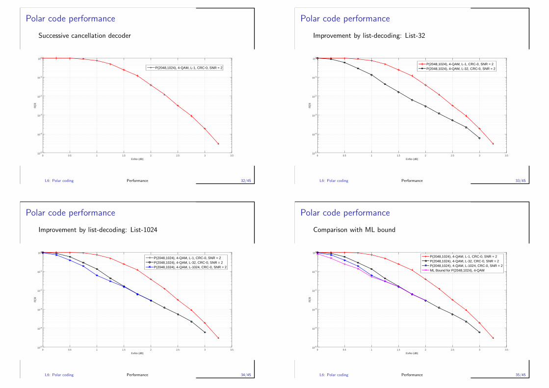
Polar code performance
Successive cancellation decoder
EsNo (dB)0 0.5 1 1.5 2 2.5 3 3.5
FE
R
10-5
10-4
10-3
10-2
10-1
100
P(2048,1024), 4-QAM, L-1, CRC-0, SNR = 2
L6: Polar coding Performance 32/45
Polar code performance
Improvement by list-decoding: List-32
EsNo (dB)0 0.5 1 1.5 2 2.5 3 3.5
FE
R
10-5
10-4
10-3
10-2
10-1
100
P(2048,1024), 4-QAM, L-1, CRC-0, SNR = 2P(2048,1024), 4-QAM, L-32, CRC-0, SNR = 2
L6: Polar coding Performance 33/45
Polar code performance
Improvement by list-decoding: List-1024
EsNo (dB)0 0.5 1 1.5 2 2.5 3 3.5
FE
R
10-5
10-4
10-3
10-2
10-1
100
P(2048,1024), 4-QAM, L-1, CRC-0, SNR = 2P(2048,1024), 4-QAM, L-32, CRC-0, SNR = 2P(2048,1024), 4-QAM, L-1024, CRC-0, SNR = 2
L6: Polar coding Performance 34/45
Polar code performance
Comparison with ML bound
EsNo (dB)0 0.5 1 1.5 2 2.5 3 3.5
FE
R
10-5
10-4
10-3
10-2
10-1
100
P(2048,1024), 4-QAM, L-1, CRC-0, SNR = 2P(2048,1024), 4-QAM, L-32, CRC-0, SNR = 2P(2048,1024), 4-QAM, L-1024, CRC-0, SNR = 2ML Bound for P(2048,1024), 4-QAM
L6: Polar coding Performance 35/45
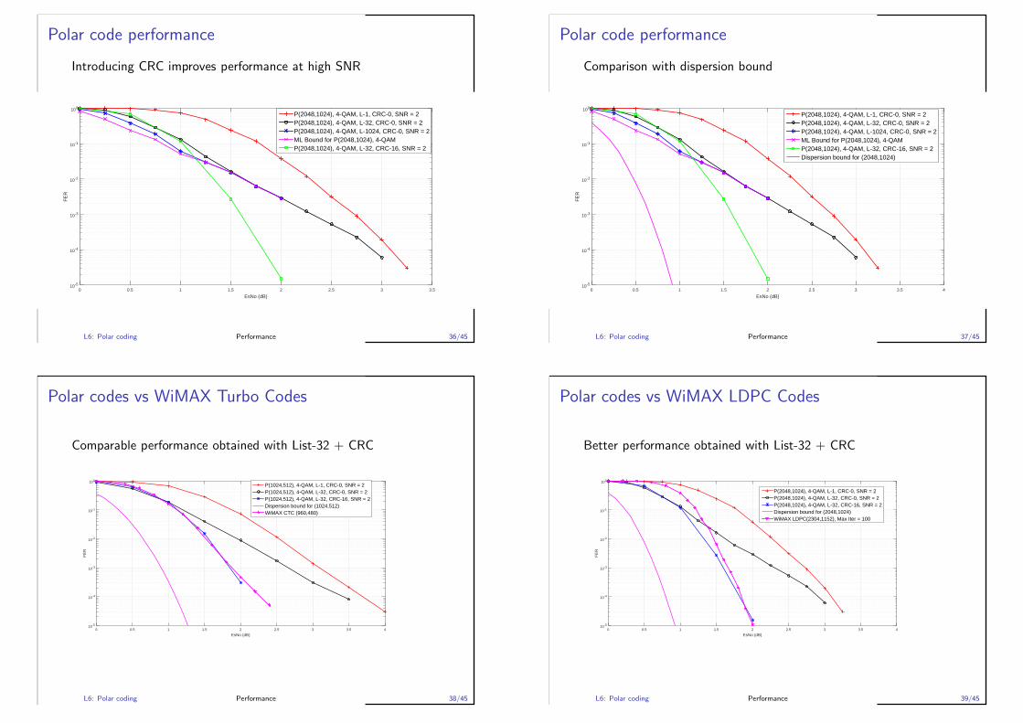
Polar code performance
Introducing CRC improves performance at high SNR
EsNo (dB)0 0.5 1 1.5 2 2.5 3 3.5
FE
R
10-5
10-4
10-3
10-2
10-1
100
P(2048,1024), 4-QAM, L-1, CRC-0, SNR = 2P(2048,1024), 4-QAM, L-32, CRC-0, SNR = 2P(2048,1024), 4-QAM, L-1024, CRC-0, SNR = 2ML Bound for P(2048,1024), 4-QAMP(2048,1024), 4-QAM, L-32, CRC-16, SNR = 2
L6: Polar coding Performance 36/45
Polar code performance
Comparison with dispersion bound
EsNo (dB)0 0.5 1 1.5 2 2.5 3 3.5 4
FE
R
10-5
10-4
10-3
10-2
10-1
100
P(2048,1024), 4-QAM, L-1, CRC-0, SNR = 2P(2048,1024), 4-QAM, L-32, CRC-0, SNR = 2P(2048,1024), 4-QAM, L-1024, CRC-0, SNR = 2ML Bound for P(2048,1024), 4-QAMP(2048,1024), 4-QAM, L-32, CRC-16, SNR = 2Dispersion bound for (2048,1024)
L6: Polar coding Performance 37/45
Polar codes vs WiMAX Turbo Codes
Comparable performance obtained with List-32 + CRC
EsNo (dB)0 0.5 1 1.5 2 2.5 3 3.5 4
FE
R
10-5
10-4
10-3
10-2
10-1
100
P(1024,512), 4-QAM, L-1, CRC-0, SNR = 2P(1024,512), 4-QAM, L-32, CRC-0, SNR = 2P(1024,512), 4-QAM, L-32, CRC-16, SNR = 2Dispersion bound for (1024,512)WiMAX CTC (960,480)
L6: Polar coding Performance 38/45
Polar codes vs WiMAX LDPC Codes
Better performance obtained with List-32 + CRC
EsNo (dB)0 0.5 1 1.5 2 2.5 3 3.5 4
FE
R
10-5
10-4
10-3
10-2
10-1
100
P(2048,1024), 4-QAM, L-1, CRC-0, SNR = 2P(2048,1024), 4-QAM, L-32, CRC-0, SNR = 2P(2048,1024), 4-QAM, L-32, CRC-16, SNR = 2Dispersion bound for (2048,1024)WiMAX LDPC(2304,1152), Max Iter = 100
L6: Polar coding Performance 39/45
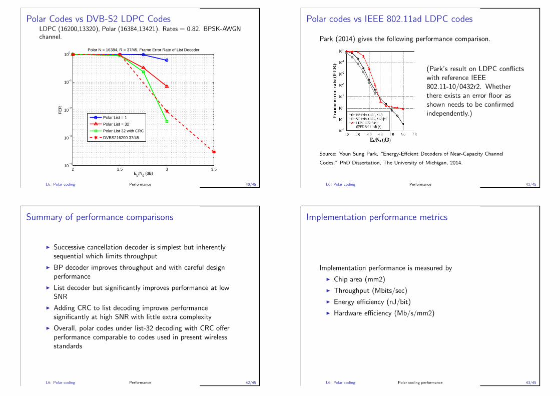
Polar Codes vs DVB-S2 LDPC CodesLDPC (16200,13320), Polar (16384,13421). Rates = 0.82. BPSK-AWGNchannel.
2 2.5 3 3.510
−4
10−3
10−2
10−1
100
Polar N = 16384, R = 37/45, Frame Error Rate of List Decoder
Eb/N
0 (dB)
FE
R
Polar List = 1
Polar List = 32
Polar List 32 with CRC
DVBS216200 37/45
L6: Polar coding Performance 40/45
Polar codes vs IEEE 802.11ad LDPC codes
Park (2014) gives the following performance comparison.
(Park’s result on LDPC conflictswith reference IEEE802.11-10/0432r2. Whetherthere exists an error floor asshown needs to be confirmedindependently.)
Source: Youn Sung Park, “Energy-Effcient Decoders of Near-Capacity Channel
Codes,” PhD Dissertation, The University of Michigan, 2014.
L6: Polar coding Performance 41/45
Summary of performance comparisons
◮ Successive cancellation decoder is simplest but inherentlysequential which limits throughput
◮ BP decoder improves throughput and with careful designperformance
◮ List decoder but significantly improves performance at lowSNR
◮ Adding CRC to list decoding improves performancesignificantly at high SNR with little extra complexity
◮ Overall, polar codes under list-32 decoding with CRC offerperformance comparable to codes used in present wirelessstandards
L6: Polar coding Performance 42/45
Implementation performance metrics
Implementation performance is measured by
◮ Chip area (mm2)
◮ Throughput (Mbits/sec)
◮ Energy efficiency (nJ/bit)
◮ Hardware efficiency (Mb/s/mm2)
L6: Polar coding Polar coding performance 43/45
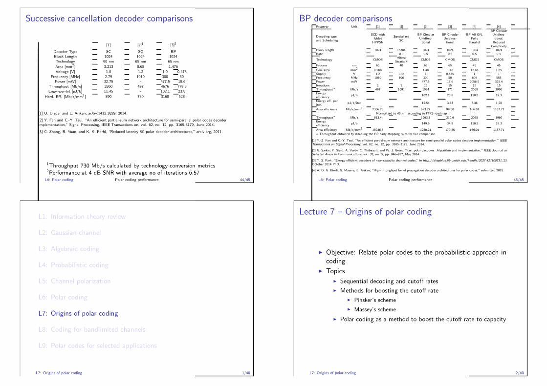
Successive cancellation decoder comparisons
[1] [2]1 [3]2
Decoder Type SC SC BP
Block Length 1024 1024 1024
Technology 90 nm 65 nm 65 nm
Area [mm2 ] 3.213 0.68 1.476
Voltage [V] 1.0 1.2 1.0 0.475
Frequency [MHz] 2.79 1010 300 50
Power [mW] 32.75 - 477.5 18.6
Throughput [Mb/s] 2860 497 4676 779.3
Engy.-per-bit [pJ/b] 11.45 - 102.1 23.8
Hard. Eff. [Mb/s/mm2 ] 890 730 3168 528
[1] O. Dizdar and E. Arıkan, arXiv:1412.3829, 2014.
[2] Y. Fan and C.-Y. Tsui, “An efficient partial-sum network architecture for semi-parallel polar codes decoderimplementation,” Signal Processing, IEEE Transactions on, vol. 62, no. 12, pp. 3165-3179, June 2014.
[3] C. Zhang, B. Yuan, and K. K. Parhi, “Reduced-latency SC polar decoder architectures,” arxiv.org, 2011.
1Throughput 730 Mb/s calculated by technology conversion metrics2Performance at 4 dB SNR with average no of iterations 6.57
L6: Polar coding Polar coding performance 44/45
BP decoder comparisonsProperty Unit [1] [2] [3] [3] [4] [4]
Decoding typeand Scheduling
SCD withfoldedHPPSN
SpecializedSC
BP CircularUnidirec-tional
BP CircularUnidirec-tional
BP All-ON,Fully
Parallel
BP CircularUnidirec-tional,
ReducedComplexity
Block length 1024 16384 1024 1024 1024 1024Rate 0.9 0.5 0.5 0.5 0.5
Technology CMOSAltera
Stratix 4CMOS CMOS CMOS CMOS
Process nm 65 40 65 65 45 45
Core area mm2 0.068 1.48 1.48 12.46 1.65Supply V 1.2 1.35 1 0.475 1 1Frequency MHz 1010 106 300 50 606 555Power mW 477.5 18.6 2056.5 328.4Iterations 1 1 15 15 15 15Throughput∗ Mb/s 497 1091 1024 171 2068 1960Energyefficiency
pJ/b 102.1 23.8 110.5 19.3
Energy eff. periter.
pJ/b/iter 15.54 3.63 7.36 1.28
Area efficiency Mb/s/mm2 7306.78 693.77 99.80 166.01 1187.71
Normalized to 45 nm according to ITRS roadmap
Throughput∗ Mb/s 613.4 1263.8 210.6 2068 1960Energyefficiency
pJ/b 149.6 34.9 110.5 19.3
Area efficiency Mb/s/mm2 18036.5 1250.21 179.85 166.01 1187.71
∗ Throughput obtained by disabling the BP early-stopping rules for fair comparison.
[1] Y.-Z. Fan and C.-Y. Tsui, “An efficient partial-sum network architecture for semi-parallel polar codes decoder implementation,” IEEETransactions on Signal Processing, vol. 62, no. 12, pp. 3165–3179, June 2014.
[2] G. Sarkis, P. Giard, A. Vardy, C. Thibeault, and W. J. Gross, “Fast polar decoders: Algorithm and implementation,” IEEE Journal onSelected Areas in Communications, vol. 32, no. 5, pp. 946–957, May 2014.
[3] Y. S. Park, “Energy-efficient decoders of near-capacity channel codes,” in http://deepblue.lib.umich.edu/handle/2027.42/108731, 23October 2014 PhD.
[4] A. D. G. Biroli, G. Masera, E. Arıkan, “High-throughput belief propagation decoder architectures for polar codes,” submitted 2015.
L6: Polar coding Polar coding performance 45/45
L1: Information theory review
L2: Gaussian channel
L3: Algebraic coding
L4: Probabilistic coding
L5: Channel polarization
L6: Polar coding
L7: Origins of polar coding
L8: Coding for bandlimited channels
L9: Polar codes for selected applications
L7: Origins of polar coding 1/40
Lecture 7 – Origins of polar coding
◮ Objective: Relate polar codes to the probabilistic approach incoding
◮ Topics
◮ Sequential decoding and cutoff rates
◮ Methods for boosting the cutoff rate
◮ Pinsker’s scheme
◮ Massey’s scheme
◮ Polar coding as a method to boost the cutoff rate to capacity
L7: Origins of polar coding 2/40
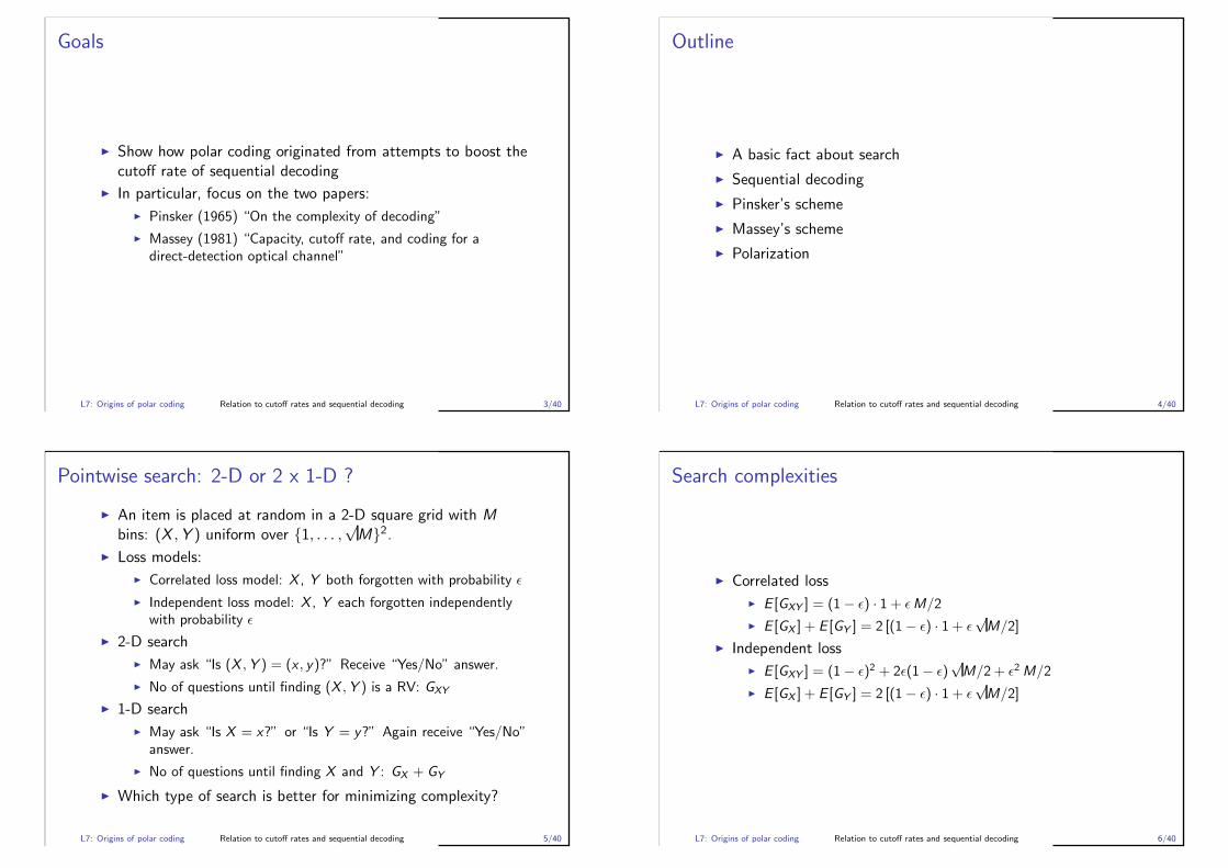
Goals
◮ Show how polar coding originated from attempts to boost thecutoff rate of sequential decoding
◮ In particular, focus on the two papers:
◮ Pinsker (1965) “On the complexity of decoding”
◮ Massey (1981) “Capacity, cutoff rate, and coding for adirect-detection optical channel”
L7: Origins of polar coding Relation to cutoff rates and sequential decoding 3/40
Outline
◮ A basic fact about search
◮ Sequential decoding
◮ Pinsker’s scheme
◮ Massey’s scheme
◮ Polarization
L7: Origins of polar coding Relation to cutoff rates and sequential decoding 4/40
Pointwise search: 2-D or 2 x 1-D ?
◮ An item is placed at random in a 2-D square grid with Mbins: (X ,Y ) uniform over {1, . . . ,
√M}2.
◮ Loss models:
◮ Correlated loss model: X , Y both forgotten with probability ǫ
◮ Independent loss model: X , Y each forgotten independentlywith probability ǫ
◮ 2-D search
◮ May ask “Is (X ,Y ) = (x , y)?” Receive “Yes/No” answer.
◮ No of questions until finding (X ,Y ) is a RV: GXY
◮ 1-D search
◮ May ask “Is X = x?” or “Is Y = y?” Again receive “Yes/No”answer.
◮ No of questions until finding X and Y : GX + GY
◮ Which type of search is better for minimizing complexity?
L7: Origins of polar coding Relation to cutoff rates and sequential decoding 5/40
Search complexities
◮ Correlated loss
◮ E [GXY ] = (1− ǫ) · 1 + ǫM/2
◮ E [GX ] + E [GY ] = 2 [(1− ǫ) · 1 + ǫ√M/2]
◮ Independent loss
◮ E [GXY ] = (1− ǫ)2 + 2ǫ(1− ǫ)√M/2 + ǫ2 M/2
◮ E [GX ] + E [GY ] = 2 [(1− ǫ) · 1 + ǫ√M/2]
L7: Origins of polar coding Relation to cutoff rates and sequential decoding 6/40
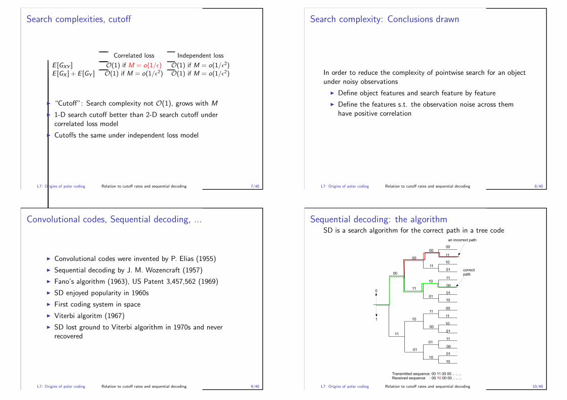
Search complexities, cutoff
Correlated loss Independent loss
E [GXY ] O(1) if M = o(1/ǫ) O(1) if M = o(1/ǫ2)E [GX ] + E [GY ] O(1) if M = o(1/ǫ2) O(1) if M = o(1/ǫ2)
◮ “Cutoff”: Search complexity not O(1), grows with M
◮ 1-D search cutoff better than 2-D search cutoff undercorrelated loss model
◮ Cutoffs the same under independent loss model
L7: Origins of polar coding Relation to cutoff rates and sequential decoding 7/40
Search complexity: Conclusions drawn
In order to reduce the complexity of pointwise search for an objectunder noisy observations
◮ Define object features and search feature by feature
◮ Define the features s.t. the observation noise across themhave positive correlation
L7: Origins of polar coding Relation to cutoff rates and sequential decoding 8/40
Convolutional codes, Sequential decoding, ...
◮ Convolutional codes were invented by P. Elias (1955)
◮ Sequential decoding by J. M. Wozencraft (1957)
◮ Fano’s algorithm (1963), US Patent 3,457,562 (1969)
◮ SD enjoyed popularity in 1960s
◮ First coding system in space
◮ Viterbi algoritm (1967)
◮ SD lost ground to Viterbi algorithm in 1970s and neverrecovered
L7: Origins of polar coding Relation to cutoff rates and sequential decoding 9/40
Sequential decoding: the algorithmSD is a search algorithm for the correct path in a tree code
L7: Origins of polar coding Relation to cutoff rates and sequential decoding 10/40
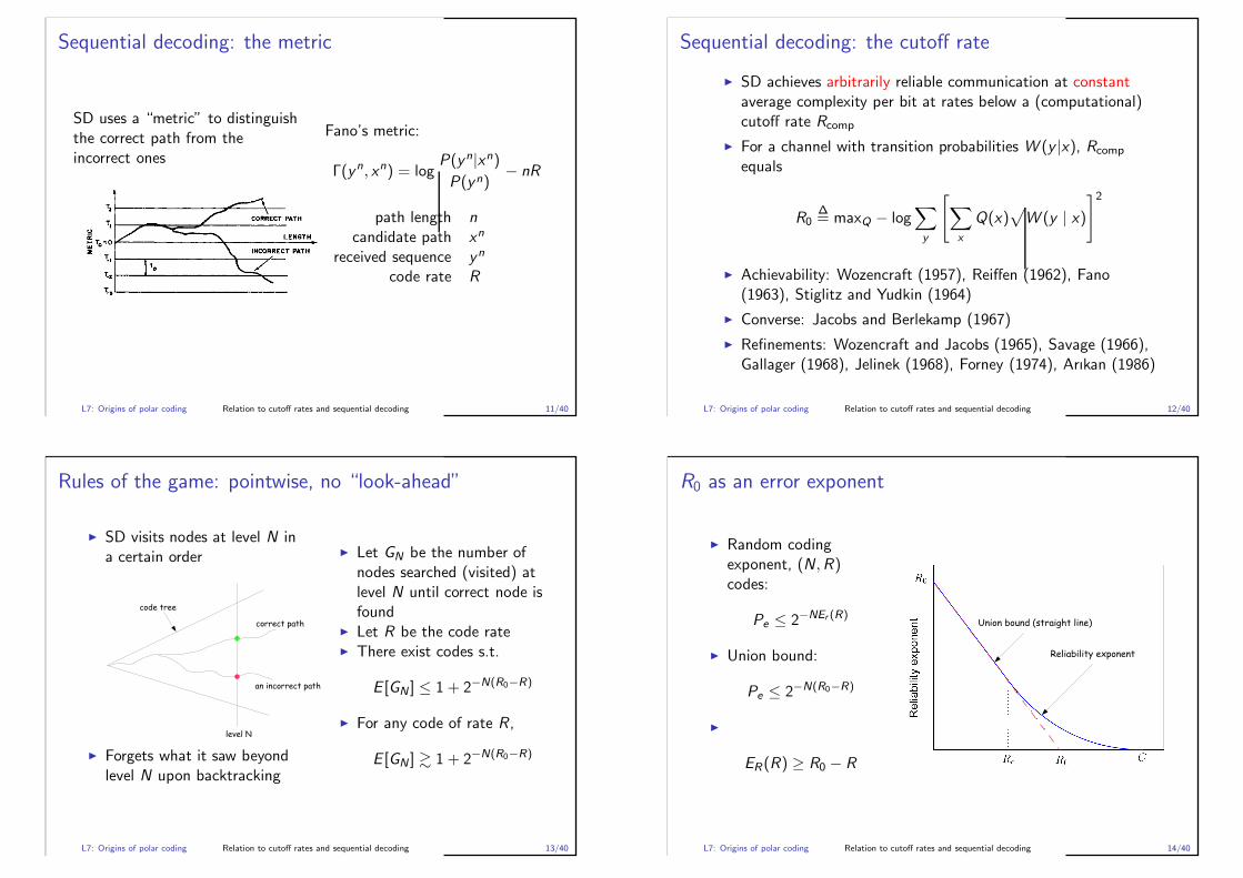
Sequential decoding: the metric
SD uses a “metric” to distinguishthe correct path from theincorrect ones
Fano’s metric:
Γ(yn, xn) = logP(yn|xn)P(yn)
− nR
path length ncandidate path xn
received sequence yn
code rate R
L7: Origins of polar coding Relation to cutoff rates and sequential decoding 11/40
Sequential decoding: the cutoff rate
◮ SD achieves arbitrarily reliable communication at constantaverage complexity per bit at rates below a (computational)cutoff rate Rcomp
◮ For a channel with transition probabilities W (y |x), Rcomp
equals
R0∆= maxQ − log
∑
y
[∑
x
Q(x)√
W (y | x)]2
◮ Achievability: Wozencraft (1957), Reiffen (1962), Fano(1963), Stiglitz and Yudkin (1964)
◮ Converse: Jacobs and Berlekamp (1967)
◮ Refinements: Wozencraft and Jacobs (1965), Savage (1966),Gallager (1968), Jelinek (1968), Forney (1974), Arıkan (1986)
L7: Origins of polar coding Relation to cutoff rates and sequential decoding 12/40
Rules of the game: pointwise, no “look-ahead”
◮ SD visits nodes at level N ina certain order
◮ Forgets what it saw beyondlevel N upon backtracking
◮ Let GN be the number ofnodes searched (visited) atlevel N until correct node isfound
◮ Let R be the code rate◮ There exist codes s.t.
E [GN ] ≤ 1 + 2−N(R0−R)
◮ For any code of rate R ,
E [GN ] & 1 + 2−N(R0−R)
L7: Origins of polar coding Relation to cutoff rates and sequential decoding 13/40
R0 as an error exponent
◮ Random codingexponent, (N,R)codes:
Pe ≤ 2−NEr (R)
◮ Union bound:
Pe ≤ 2−N(R0−R)
◮
ER(R) ≥ R0 − R
L7: Origins of polar coding Relation to cutoff rates and sequential decoding 14/40
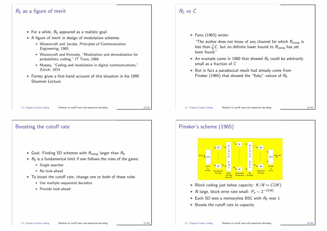
R0 as a figure of merit
◮ For a while, R0 appeared as a realistic goal
◮ A figure of merit in design of modulation schemes
◮ Wozencraft and Jacobs, Principles of CommunicationEngineering, 1965
◮ Wozencraft and Kennedy, “Modulation and demodulation forprobabilistic coding,” IT Trans.,1966
◮ Massey, “Coding and modulation in digital communications,”Zurich, 1974
◮ Forney gives a first-hand account of this situation in his 1995Shannon Lecture
L7: Origins of polar coding Relation to cutoff rates and sequential decoding 15/40
R0 vs C
◮ Fano (1963) wrote:
“The author does not know of any channel for which Rcomp isless than 1
2C , but no definite lower bound to Rcomp has yetbeen found.”
◮ An example came in 1980 that showed R0 could be arbitrarilysmall as a fraction of C
◮ But in fact a paradoxical result had already come fromPinsker (1965) that showed the “flaky” nature of R0
L7: Origins of polar coding Relation to cutoff rates and sequential decoding 16/40
Boosting the cutoff rate
◮ Goal: Finding SD schemes with Rcomp larger than R0
◮ R0 is a fundamental limit if one follows the rules of the game:
◮ Single searcher
◮ No look-ahead
◮ To boost the cutoff rate, change one or both of these rules
◮ Use multiple sequential decoders
◮ Provide look-ahead
L7: Origins of polar coding Relation to cutoff rates and sequential decoding 17/40
Pinsker’s scheme (1965)
◮ Block coding just below capacity: K/N ≈ C (W )
◮ N large, block error rate small: Pe ∼ 2−O(N)
◮ Each SD sees a memoryless BSC with R0 near 1
◮ Boosts the cutoff rate to capacity
L7: Origins of polar coding Relation to cutoff rates and sequential decoding 18/40
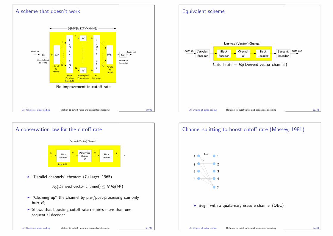
A scheme that doesn’t work
No improvement in cutoff rate
L7: Origins of polar coding Relation to cutoff rates and sequential decoding 19/40
Equivalent scheme
Cutoff rate = R0(Derived vector channel)
L7: Origins of polar coding Relation to cutoff rates and sequential decoding 20/40
A conservation law for the cutoff rate
◮ “Parallel channels” theorem (Gallager, 1965)
R0(Derived vector channel) ≤ N R0(W )
◮ “Cleaning up” the channel by pre-/post-processing can onlyhurt R0
◮ Shows that boosting cutoff rate requires more than onesequential decoder
L7: Origins of polar coding Relation to cutoff rates and sequential decoding 21/40
Channel splitting to boost cutoff rate (Massey, 1981)
◮ Begin with a quaternary erasure channel (QEC)
L7: Origins of polar coding Relation to cutoff rates and sequential decoding 22/40

Channel splitting to boost cutoff rate (Massey, 1981)
◮ Relabel the inputs
L7: Origins of polar coding Relation to cutoff rates and sequential decoding 23/40
Channel splitting to boost cutoff rate (Massey, 1981)
◮ Split the QEC into two binary erasure channels (BEC)
◮ BECs fully correlated: erasures occur jointly
L7: Origins of polar coding Relation to cutoff rates and sequential decoding 24/40
Capacity, cutoff rate for one QEC vs two BECs
Ordinary coding of QEC
C (QEC) = 2(1 − ǫ)
R0(QEC) = log 41+3ǫ
E QEC D
Independent coding of BECs
C (BEC) = (1− ǫ)
R0(BEC) = log 21+ǫ
E BEC D
E BEC D
L7: Origins of polar coding Relation to cutoff rates and sequential decoding 25/40
Cutoff rate improvement by splitting
0 0.1 0.2 0.3 0.4 0.5 0.6 0.7 0.8 0.9 10
0.2
0.4
0.6
0.8
1
1.2
1.4
1.6
1.8
2
Erasure probability ε
Cap
acity
, cut
off r
ate
(bits
)
Cutoff rate of QEC
Cutoff rate of BEC
Sum cutoff rate after splitting
Capacity of QEC
L7: Origins of polar coding Relation to cutoff rates and sequential decoding 26/40
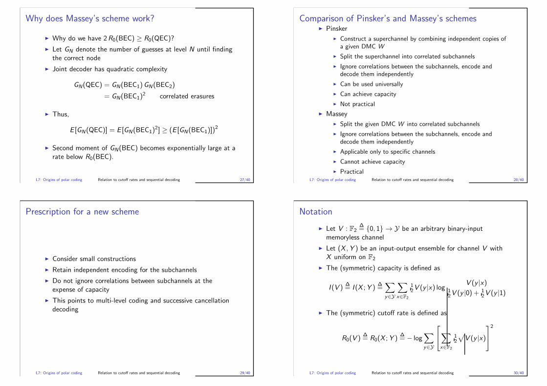
Why does Massey’s scheme work?
◮ Why do we have 2R0(BEC) ≥ R0(QEC)?
◮ Let GN denote the number of guesses at level N until findingthe correct node
◮ Joint decoder has quadratic complexity
GN(QEC) = GN(BEC1)GN(BEC2)
= GN(BEC1)2 correlated erasures
◮ Thus,
E [GN(QEC)] = E [GN(BEC1)2] ≥ (E [GN(BEC1)])
2
◮ Second moment of GN(BEC) becomes exponentially large at arate below R0(BEC).
L7: Origins of polar coding Relation to cutoff rates and sequential decoding 27/40
Comparison of Pinsker’s and Massey’s schemes◮ Pinsker
◮ Construct a superchannel by combining independent copies ofa given DMC W
◮ Split the superchannel into correlated subchannels
◮ Ignore correlations between the subchannels, encode anddecode them independently
◮ Can be used universally
◮ Can achieve capacity
◮ Not practical
◮ Massey
◮ Split the given DMC W into correlated subchannels
◮ Ignore correlations between the subchannels, encode anddecode them independently
◮ Applicable only to specific channels
◮ Cannot achieve capacity
◮ PracticalL7: Origins of polar coding Relation to cutoff rates and sequential decoding 28/40
Prescription for a new scheme
◮ Consider small constructions
◮ Retain independent encoding for the subchannels
◮ Do not ignore correlations between subchannels at theexpense of capacity
◮ This points to multi-level coding and successive cancellationdecoding
L7: Origins of polar coding Relation to cutoff rates and sequential decoding 29/40
Notation
◮ Let V : F2∆= {0, 1} → Y be an arbitrary binary-input
memoryless channel
◮ Let (X ,Y ) be an input-output ensemble for channel V withX uniform on F2
◮ The (symmetric) capacity is defined as
I (V )∆= I (X ;Y )
∆=
∑
y∈Y
∑
x∈F2
12V (y |x) log V (y |x)
12V (y |0) + 1
2V (y |1)
◮ The (symmetric) cutoff rate is defined as
R0(V )∆= R0(X ;Y )
∆= − log
∑
y∈Y
∑
x∈F2
12
√
V (y |x)
2
L7: Origins of polar coding Relation to cutoff rates and sequential decoding 30/40

Basic module for a low-complexity scheme
Combine two copies of W
+
U2
U1
G2
W
W
Y2
Y1
X2
X1
and split to create two bit-channels
W1 : U1 → (Y1,Y2)
W2 : U2 → (Y1,Y2,U1)
L7: Origins of polar coding Relation to cutoff rates and sequential decoding 31/40
The first bit-channel W1
W1 : U1 → (Y1,Y2)
+
random U2
U1
W
W
Y2
Y1
C (W1) = I (U1;Y1,Y2)
L7: Origins of polar coding Relation to cutoff rates and sequential decoding 32/40
The second bit-channel W2
W2 : U2 → (Y1,Y2,U1)
+
U2
U1
W
W
Y2
Y1
C (W2) = I (U2;Y1,Y2,U1)
L7: Origins of polar coding Relation to cutoff rates and sequential decoding 33/40
The 2x2 transformation is information lossless
◮ With independent, uniform U1,U2,
I (W−) = I (U1;Y1Y2),
I (W+) = I (U2;Y1Y2U1).
◮ Thus,
I (W−) + I (W+) = I (U1U2;Y1Y2)
= 2I (W ),
◮ and I (W−) ≤ I (W ) ≤ I (W+).
L7: Origins of polar coding Relation to cutoff rates and sequential decoding 34/40
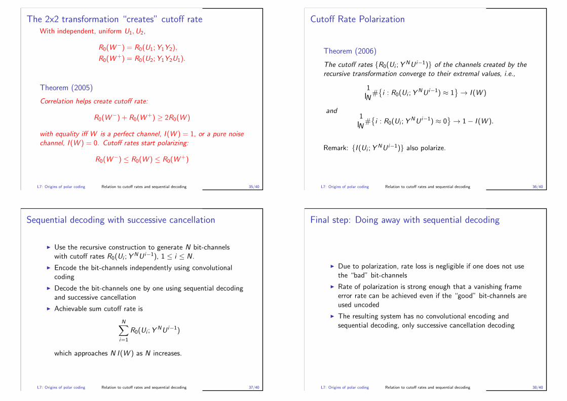
The 2x2 transformation “creates” cutoff rateWith independent, uniform U1,U2,
R0(W−) = R0(U1;Y1Y2),
R0(W+) = R0(U2;Y1Y2U1).
Theorem (2005)
Correlation helps create cutoff rate:
R0(W−) + R0(W
+) ≥ 2R0(W )
with equality iff W is a perfect channel, I (W ) = 1, or a pure noisechannel, I (W ) = 0. Cutoff rates start polarizing:
R0(W−) ≤ R0(W ) ≤ R0(W
+)
L7: Origins of polar coding Relation to cutoff rates and sequential decoding 35/40
Cutoff Rate Polarization
Theorem (2006)
The cutoff rates {R0(Ui ;YNU i−1)} of the channels created by the
recursive transformation converge to their extremal values, i.e.,
1
N#{i : R0(Ui ;Y
NU i−1) ≈ 1}→ I (W )
and1
N#{i : R0(Ui ;Y
NU i−1) ≈ 0}→ 1− I (W ).
Remark: {I (Ui ;YNU i−1)} also polarize.
L7: Origins of polar coding Relation to cutoff rates and sequential decoding 36/40
Sequential decoding with successive cancellation
◮ Use the recursive construction to generate N bit-channelswith cutoff rates R0(Ui ;Y
NU i−1), 1 ≤ i ≤ N.
◮ Encode the bit-channels independently using convolutionalcoding
◮ Decode the bit-channels one by one using sequential decodingand successive cancellation
◮ Achievable sum cutoff rate is
N∑
i=1
R0(Ui ;YNU i−1)
which approaches N I (W ) as N increases.
L7: Origins of polar coding Relation to cutoff rates and sequential decoding 37/40
Final step: Doing away with sequential decoding
◮ Due to polarization, rate loss is negligible if one does not usethe “bad” bit-channels
◮ Rate of polarization is strong enough that a vanishing frameerror rate can be achieved even if the “good” bit-channels areused uncoded
◮ The resulting system has no convolutional encoding andsequential decoding, only successive cancellation decoding
L7: Origins of polar coding Relation to cutoff rates and sequential decoding 38/40

Polar coding
To communicate at rate R < I (W ):
◮ Pick N, and K = NR good indices i such that I (Ui ;YNU i−1)
is high,
◮ let the transmitter set Ui to be uncoded binary data for goodindices, and set Ui to random but publicly known values forthe rest,
◮ let the receiver decode the Ui successively: U1 from Y N ; Ui
from Y NU i−1.
L7: Origins of polar coding Relation to cutoff rates and sequential decoding 39/40
Polar coding complexity and performance
Theorem (2007)
With the particular one-to-one mapping described here and withthe successive cancellation decoding
◮ polarization codes are ‘I (W ) achieving’,
◮ encoding complexity is N logN,
◮ decoding complexity is N logN,
◮ probability of error decays like 2−√N (with E. Telatar, 2008).
L7: Origins of polar coding Relation to cutoff rates and sequential decoding 40/40
L1: Information theory review
L2: Gaussian channel
L3: Algebraic coding
L4: Probabilistic coding
L5: Channel polarization
L6: Polar coding
L7: Origins of polar coding
L8: Coding for bandlimited channels
L9: Polar codes for selected applications
L8: Coding for bandlimited channels 1/37
Lecture 8 – Coding for bandlimited channels
◮ Objective: To discuss coding for bandlimited channels ingeneral and with polar coding in particular
◮ Topics
◮ Bit interleaved coded modulation (BICM)
◮ Multi-level coding and modulation (MLCM)
◮ Lattice coding
◮ Direct polarization approach
L8: Coding for bandlimited channels 2/37
The AWGN Channel
The AWGN channel is a continuous-time channel
Y (t) = X (t) + N(t)
such that the input X (t) is a random process bandlimited to Wsubject to a power constraint X 2(t) ≤ P , and N(t) is whiteGaussian noise with power spectral density N0/2.
L8: Coding for bandlimited channels Background 3/37
Capacity
Shannon’s formula gives the capacity of the AWGN channel as
C[b/s] = W log2(1 + P/WN0) (bits/s)
L8: Coding for bandlimited channels Background 4/37
Signal Design Problem
The continuous time and real-number interface of the AWGNchannel is inconvenient for digital communications.
◮ Need to convert from continuous to discrete-time
◮ Need to convert from real numbers to a binary interface
L8: Coding for bandlimited channels Background 5/37
Discrete Time Model
An AWGN channel of bandwidth W gives rise to 2W independentdiscrete time channels per second with input-output mapping
Y = X + N
◮ X is a random variable with mean 0 and energyE [X 2] ≤ P/2W
◮ N is Gaussian noise with 0-mean and energy N0/2.
◮ It is customary to normalize the signal energies to joules per 2dimensions and define
Es = P/W Joules/2D
as signal energy (per two dimensions).
◮ One defines the the signal-to-noise ratio as Es/N0.
L8: Coding for bandlimited channels Background 6/37
Capacity
The capacity of the discrete-time AWGN channel is given by
C =1
2log2(1 + Es/N0), (bits/D),
achieved by i.i.d. Gaussian inputs X ∼ N(0,Es/2) per dimension.
L8: Coding for bandlimited channels Background 7/37
Signal Design Problem
Now, we need a digital interface instead of real-valued inputs.
◮ Select a subset A ⊂ Rn as the “signal set” or “modulationalphabet”.
◮ Finding a signal set with good Euclidean distance propertiesand other desirable features is the “signal design” problem.
◮ Typically, the dimension n is 1 or 2.
L8: Coding for bandlimited channels Background 8/37
Separation of coding and modulation
◮ Each constellation A has a capacity CA (bits/D) which is afunction of Es/N0.
◮ The spectral efficiency ρ (bits/D) has to satisfy
ρ < CA(Es/N0)
at the operating Es/N0.
◮ The spectral efficiency is the product of two terms
ρ = R × log2(|A|)dim(A)
where R (dimensionless) is the rate of the FEC.
◮ For a given ρ, there any many choices w.r.t. R and A.
L8: Coding for bandlimited channels Background 9/37
Cutoff rate: A simple measure of reliability
Each constellation A has a cutoff rate R0,A (bits/D) which is afunction of Es/N0 such that through random coding one canguarantee the existence of coding and modulation schemes withprobability of frame error
Pe < 2−N[R0,A(Es/N0)−ρ]
where N is the frame length in modulation symbols.
L8: Coding for bandlimited channels Background 10/37
Sequential decoding and cutoff rate
◮ Sequential decoding (Wozencraft, 1957) is a decodingalgorithm for convolutional codes that can achieve spectralefficiencies as high as the cutoff rate at constant averagecomplexity per decoded bit.
◮ The difference between cutoff rate and capacity at high Es/N0
is less than 3 dB.
◮ This was regarded as the solution of the coding andmodulation problem in early 70s and interest in the problemwaned. (See Forney 1995 Shannon Lecture for this story.)
◮ Polar coding grew out of attempts to improve the cutoff rateof channels by simple combining and splitting operations.
L8: Coding for bandlimited channels Background 11/37
M-ary Pulse Amplitude Modulation
A 1-D signal set with A = {±α,±3α, . . . ,±(M − 1)}.◮ Average energy: Es = 2α2(M2 − 1)/3 (Joules/2D)
◮ Consider the capacity, cutoff rate
L8: Coding for bandlimited channels Background 12/37
Capacity of M-PAM
Es/N0 (db)-10 0 10 20 30 40 50
Cap
acity
(bi
ts)
0
1
2
3
4
5
6
7
8
9Capacity with PAM
PAM-2PAM-4PAM-8PAM-16PAM-32PAM-64PAM-128Shannon Limit
M-PAM is good enough from a capacity viewpoint.L8: Coding for bandlimited channels Background 13/37
Cutoff rate of M-PAM
Es/N0 (db)-10 0 10 20 30 40 50
Cut
off r
ate
(bits
)
0
1
2
3
4
5
6
7
8
9Cutoff rate with PAM
PAM-2PAM-4PAM-8PAM-16PAM-32PAM-64PAM-128PAM-256PAM-512PAM-1024Shannon capacityShannon cutoff rateGaussian input cutoff rate
M-PAM is satisfactory also in terms of cutoff rate.L8: Coding for bandlimited channels Background 14/37
Conventional approach
Given a target spectral efficiency ρ and a target error rate Pe at aspecific Es/No ,
◮ select M large enough so that M-PAM capacity is closeenough to the Shannon capacity at the given Es/No
◮ apply coding external to modulation to achieve the desired Pe
Such separation of coding and modulation was first challengedsuccessfully by Ungerboeck (1981).
However, with the advent of powerful codes at affordablecomplexity, there is a return to the conventional designmethodology.
L8: Coding for bandlimited channels Background 15/37
How does it work in practice?
Es/No in dB4 5 6 7 8 9 10 11 12 13
FE
R
10-5
10-4
10-3
10-2
10-1
100WiMAX CTC Codes: Fixed Spectral Efficiency, Different Modulation
CTC(576,432), 16-QAMCTC(864,432), 64-QAM
Gap to Shannonabout 3 dB at FER 1E-3
It takes 144 symbols to carrythe payload in both cases.
Spectral efficiency = 3 b/2Dfor both cases.
Provides a coding gain of 4.8 dBover uncoded transmission
Theory and practice don’t match here!L8: Coding for bandlimited channels Background 16/37
Why change modulation instead of just the code rate?
◮ Suppose we fix the modulation as 64-QAM and wish todeliver data at spectral efficiencies 1, 2, 3, 4, 5 b/2D.
◮ We would need a coding scheme that works well at rates 1/6,1/3, 1/2, 2/3, 5/6.
◮ The inability of delivering high quality coding over a widerange of rates forces one to change the order of modulation.
◮ The difficulty here is practical: it is a challenge to have acoding scheme that works well over all rates from 0 to 1.
L8: Coding for bandlimited channels Background 17/37
Alternative: Fixed code, variable modulation
Es/No in dB0 2 4 6 8 10 12 14 16 18
FE
R
10-5
10-4
10-3
10-2
10-1
100WiMAX: Same rate-3/4 code with different order QAM modulations
CTC(576,432), 4-QAMCTC(576,432), 16-QAMCTC(576,432), 64-QAM
Gap to Shannon limit widens slightly with increasing modulation order but in general good agreement.
spec. eff. 4.5spec. eff. 3spec. eff. 1.5
L8: Coding for bandlimited channels Background 18/37
Polar coding and modulation
Polar codes can be applied to modulation in at least three differentways.
◮ Direct polarization
◮ Multi-level techniques
◮ Polar lattices
◮ BICM
L8: Coding for bandlimited channels polar 19/37
Direct Method
Idea: Given a system with q-ary modulation, treat it as an ordinaryq-ary input memoryless channel and apply a suitable polarizationtransform.
Theory of q-ary polarization exists.
◮ Sasoglu, E., E. Telatar, and E. Arıkan. “Polarization forarbitrary discrete memoryless channels.” IEEE ITW 2009.
◮ Sahebi, A. G. and S. S. Pradhan, “Multilevel polarization ofpolar codes over arbitrary discrete memoryless channels.”IEEE Allerton, 2011.
◮ Park, W.-C. and A. Barg. “Polar codes for q-ary channels,”IEEE Trans. Inform. Theory, 2013.
◮ ...
L8: Coding for bandlimited channels polar 20/37
Direct Method
The difficulty with the direct approach is complexity of decoding.
G. Montorsi’s ADBP is a promising approach for reducing thecomplexity here.
L8: Coding for bandlimited channels polar 21/37
Multi-Level Modulation (Imai and Hirakawa, 1977)
Represent (if possible) each channel input symbol as a vectorX = (X1,X2, . . . ,Xr ); then the capacity can be written as a sum ofcapacities of smaller channels by the chain rule:
I (X ;Y ) = I (X1,X2, . . . ,Xr ;Y )
=r∑
i=1
I (Xi ;Y |X1, . . . ,Xi−1).
This splits the original channel into r parallel channels, which areencoded independently and decoded using successive cancellationdecoding.
Polarization is a natural complement to MLM.
L8: Coding for bandlimited channels polar 22/37
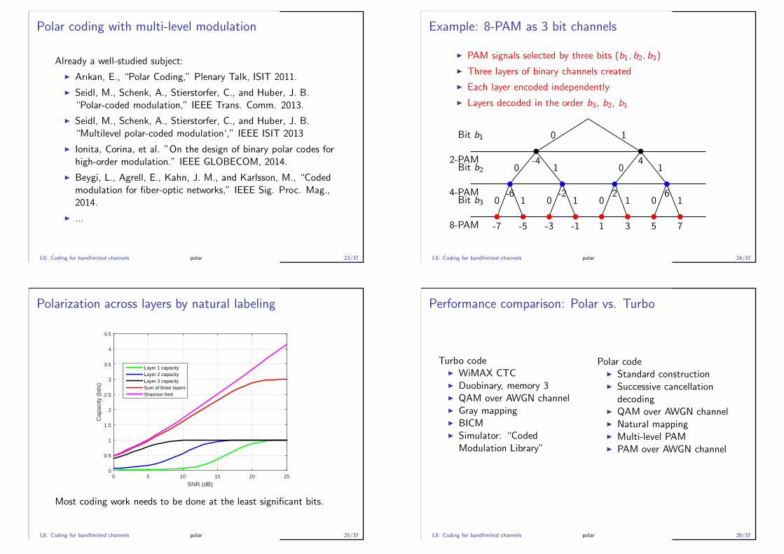
Polar coding with multi-level modulation
Already a well-studied subject:
◮ Arıkan, E., “Polar Coding,” Plenary Talk, ISIT 2011.
◮ Seidl, M., Schenk, A., Stierstorfer, C., and Huber, J. B.“Polar-coded modulation,” IEEE Trans. Comm. 2013.
◮ Seidl, M., Schenk, A., Stierstorfer, C., and Huber, J. B.“Multilevel polar-coded modulation‘,” IEEE ISIT 2013
◮ Ionita, Corina, et al. ”On the design of binary polar codes forhigh-order modulation.” IEEE GLOBECOM, 2014.
◮ Beygi, L., Agrell, E., Kahn, J. M., and Karlsson, M., “Codedmodulation for fiber-optic networks,” IEEE Sig. Proc. Mag.,2014.
◮ ...
L8: Coding for bandlimited channels polar 23/37
Example: 8-PAM as 3 bit channels
◮ PAM signals selected by three bits (b1, b2, b3)
◮ Three layers of binary channels created
◮ Each layer encoded independently
◮ Layers decoded in the order b3, b2, b1
Bit b2 0 1 10
-6 -2 2 64-PAM
Bit b1 0 1
-4 42-PAM
-7 -5 -3 -1 1 3 5 7
0 1 0 1 0 1 0 1Bit b3
8-PAM
L8: Coding for bandlimited channels polar 24/37
Polarization across layers by natural labeling
SNR (dB)0 5 10 15 20 25
Cap
acity
(bi
ts)
0
0.5
1
1.5
2
2.5
3
3.5
4
4.5
Layer 1 capacityLayer 2 capacityLayer 3 capacitySum of three layersShannon limit
Most coding work needs to be done at the least significant bits.
L8: Coding for bandlimited channels polar 25/37
Performance comparison: Polar vs. Turbo
Turbo code◮ WiMAX CTC◮ Duobinary, memory 3◮ QAM over AWGN channel◮ Gray mapping◮ BICM◮ Simulator: “Coded
Modulation Library”
Polar code◮ Standard construction◮ Successive cancellation
decoding◮ QAM over AWGN channel◮ Natural mapping◮ Multi-level PAM◮ PAM over AWGN channel
L8: Coding for bandlimited channels polar 26/37

Example: 8-PAM as 3 bit channels
◮ PAM signals selected by three bits (b1, b2, b3)
◮ Three layers of binary channels created
◮ Each layer encoded independently
◮ Layers decoded in the order b3, b2, b1
Bit b2 0 1 10
-6 -2 2 64-PAM
Bit b1 0 1
-4 42-PAM
-7 -5 -3 -1 1 3 5 7
0 1 0 1 0 1 0 1Bit b3
8-PAM
L8: Coding for bandlimited channels polar 27/37
Multi-layering jump-starts polarization
0 5 10 15 200
0.5
1
1.5
2
2.5
3
3.5
SNR (dB)
Cap
acity
(bi
ts)
Layer 1 capacityLayer 2 capacityLayer 3 capacitySum of three layersShannon limit
L8: Coding for bandlimited channels polar 28/37
4-QAM, Rate 1/2
−1 0 1 2 3 4 5 610
−6
10−5
10−4
10−3
10−2
10−1
100
EbNo (dB)
FE
R
Polar(512,256) 4−QAMPolar(1024,512) 4−QAMCTC(480,240) 4−QAMCTC(960,480) 4−QAM
Turbo
Polar
L8: Coding for bandlimited channels polar 29/37
16-QAM, Rate 3/4
3 3.5 4 4.5 5 5.5 6 6.5 7 7.5 8 8.510
−6
10−5
10−4
10−3
10−2
10−1
100
EbNo (dB)
FE
R
Polar(512,384) 16−QAMCTC(192,144) 16−QAMCTC(384,288) 16−QAMCTC(576,432) 16−QAM
L8: Coding for bandlimited channels polar 30/37

64-QAM, Rate 5/6
7.5 8 8.5 9 9.5 10 10.5 11 11.5 12 12.5 1310
−5
10−4
10−3
10−2
10−1
100
EbNo (dB)
FE
R
Polar(768,640) 64−QAMPolar(384,320) 64−QAMCTC(576,480) 64−QAM
L8: Coding for bandlimited channels polar 31/37
Complexity comparison: 64-QAM, Rate 5/6
Average decoding time in milliseconds per codeword (ms/cw)
Eb/N0 CTC(576,432) Polar(768,640) Polar(384,320)
10 dB 6.23 0.92 0.4811 dB 1.83 1.01 0.53
Polar codes show a complexity advantage against CTC codes.
Both decoders implemented as MATLAB mex functions. Polar decoder is a successive
cancellation decoder. CTC decoder is a public domain decoder (CML). Profiling done
by MATLAB Profiler. Iteration limit for CTC decoder was 10; average no of iterations
was 10 at 10 dB and 3.3 at 11 dB. CTC decoder used a linear approximation to
log-MAP while polar decoder used exact log-MAP.
L8: Coding for bandlimited channels polar 32/37
Lattices and polar coding
Yan, Cong, and Liu explored the connection between lattices andpolar coding.
◮ Yan, Yanfei, and L. Cong, “A construction of lattices frompolar codes.” IEEE 2012 ITW.
◮ Yan, Yanfei, Ling Liu, Cong Ling, and Xiaofu Wu.“Construction of capacity-achieving lattice codes: Polarlattices.” arXiv preprint arXiv:1411.0187 (2014)
L8: Coding for bandlimited channels polar 33/37
Lattices and polar coding
Yan et al used the Barnes-Wall lattice contructions such as
BW16 = RM(1, 4) + 2RM(3, 4) + 4(Z16)
as a template for constructing polar lattices of the type
P16 = P(1, 4) + 2P(3, 4) + 4(Z16)
and demonstrated by simulations that polar lattices perform better.
L8: Coding for bandlimited channels polar 34/37
BICM
BICM [Zehavi, 1991], [Caire, Taricco, Biglieri, 1998] is thedominant technique in modern wireless standards such as LTE.
As in MLM, BICM splits the channel input symbols into a vectorX = (X1,X2, . . . ,Xr ) but strives to do so such that
I (X ;Y ) = I (X1,X2, . . . ,Xr ;Y )
=
r∑
i=1
I (Xi ;Y |X1, . . . ,Xi−1)
≈r∑
i=1
I (Xi ;Y ).
L8: Coding for bandlimited channels polar 35/37
BICM vs Multi Level Modulation
Why has BICM won over MLM and other techniques in practice?
◮ MLM is provably capacity-achieving; BICM is suboptimal butthe rate penalty is tolerable.
◮ MLM has to do delicate rate-matching at individual layers,which is difficult with turbo and LDPC codes.
◮ BICM is well-matched to iterative decoding methods usedwith turbo and LDPC codes.
◮ MLM suffers extra latency due to multi-stage decoding(mitigated in part by the lack of need for protecting the upperlayers by long codes)
◮ With MLM, the overall code is split into shorter codes whichweakens performance (one may mix and match the blocklengths of each layer to alleviate this problem).
L8: Coding for bandlimited channels polar 36/37
BICM and Polar Coding
This subject, too, has been studied in connection with polar codes.
◮ Mahdavifar, H. and El-Khamy, M. and Lee, J. and Kang, I.,“Polar Coding for Bit-Interleaved Coded Modulation,” IEEETrans. Veh. Tech., 2015.
◮ Afser, H., N. Tirpan, H. Delic, and M. Koca, “Bit-interleavedpolar-coded modulation,” Proc. IEEE WCNC, 2014.
◮ Chen, Kai, Kai Niu, and Jia-Ru Lin. “An efficient design ofbit-interleaved polar coded modulation.” IEEE PIMRC 2013.
◮ ...
L8: Coding for bandlimited channels polar 37/37
L1: Information theory review
L2: Gaussian channel
L3: Algebraic coding
L4: Probabilistic coding
L5: Channel polarization
L6: Polar coding
L7: Origins of polar coding
L8: Coding for bandlimited channels
L9: Polar codes for selected applications
L9: Polar codes for selected applications 1/27

Lecture 9 – Polar codes for selected applications
◮ Objective: Review the literature on polar coding for selectedapplications
◮ Topics
◮ 60 GHz wireless
◮ Optical access networks
◮ 5G
◮ Ultra reliable low latency communications (URLLC)
◮ Machine type communications (MTC)
◮ 5G channel coding at Gb/s throughput
L9: Polar codes for selected applications 2/27
Millimeter Wave 60 GHz Communications
◮ 7 GHz of bandwidth available (57-64 GHz allocated in the US)
◮ Free-space path loss (4πd/λ)2 is high at λ = 5 mm butcompensated by large antenna arrays.
◮ Propagation range limited severely by O2 absorption. Cellsconfined to rooms.
L9: Polar codes for selected applications 60 GHz Wireless 3/27
Millimeter Wave 60 GHz Communications
◮ Recent IEEE 802.11.ad Wi-Fi standard operates at 60 GHzISM band and uses an LDPC code with block length 672 bits,rates 1/2, 5/8, 3/4, 13/16.
◮ Two papers compare polar codes that study polar coding for60 GHz applications:
◮ Z. Wei, B. Li, and C. Zhao, “On the polar code for the 60 GHzmillimeter-wave systems,” EURASIP, JWCN, 2015.
◮ Youn Sung Park, “Energy-Effcient Decoders of Near-CapacityChannel Codes,” PhD Dissertation, The University ofMichigan, 2014.
L9: Polar codes for selected applications 60 GHz Wireless 4/27
Millimeter Wave 60 GHz Communications
Wei et al compare polar codes with the LDPC codes used in thestandard using a nonlinear channel model
Wei, B. Li, and C. Zhao, “On the polar code for the 60 GHz millimeter-wave
systems,” EURASIP, JWCN, 2015.
L9: Polar codes for selected applications 60 GHz Wireless 5/27
Millimeter Wave 60 GHz Communications
Wei et al compare polar codes with the LDPC codes used in thestandard using a nonlinear channel model
Wei, B. Li, and C. Zhao, “On the polar code for the 60 GHz millimeter-wave
systems,” EURASIP, JWCN, 2015.
L9: Polar codes for selected applications 60 GHz Wireless 6/27
Millimeter Wave 60 GHz Communications
Wei et al compare polar codes with the LDPC codes used in thestandard using a nonlinear channel model
Wei, B. Li, and C. Zhao, “On the polar code for the 60 GHz millimeter-wave
systems,” EURASIP, JWCN, 2015.
L9: Polar codes for selected applications 60 GHz Wireless 7/27
Polar codes vs IEEE 802.11ad LDPC codes
Park (2014) gives the following performance comparison.
(Park’s result on LDPC conflictswith reference IEEE802.11-10/0432r2. Whetherthere exists an error floor asshown needs to be confirmedindependently.)
Source: Youn Sung Park, “Energy-Effcient Decoders of Near-Capacity Channel
Codes,” PhD Dissertation, The University of Michigan, 2014.
L9: Polar codes for selected applications 60 GHz Wireless 8/27
Polar codes vs IEEE 802.11ad LDPC codes
In terms of implementation complexity and throughput, Park(2014) gives the following figures.
Source: Youn Sung Park, “Energy-Efficient Decoders of Near-Capacity Channel
Codes,” PhD Dissertation, The University of Michigan, 2014.
L9: Polar codes for selected applications 60 GHz Wireless 9/27
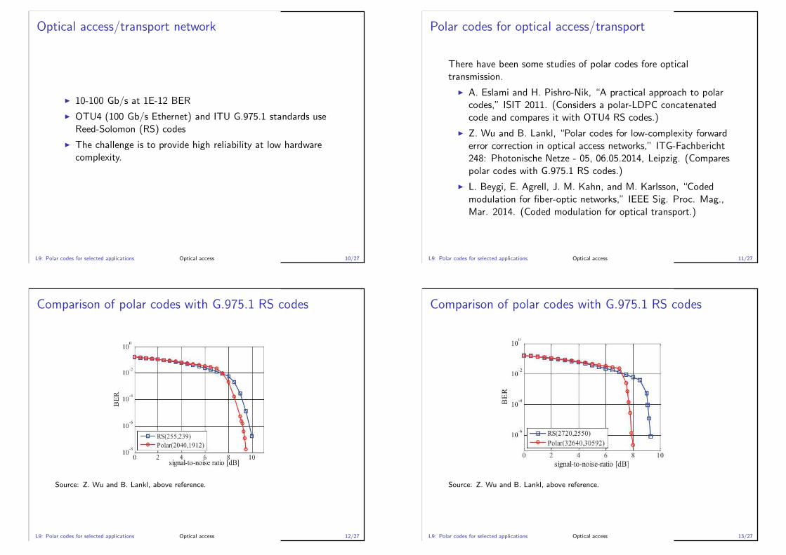
Optical access/transport network
◮ 10-100 Gb/s at 1E-12 BER
◮ OTU4 (100 Gb/s Ethernet) and ITU G.975.1 standards useReed-Solomon (RS) codes
◮ The challenge is to provide high reliability at low hardwarecomplexity.
L9: Polar codes for selected applications Optical access 10/27
Polar codes for optical access/transport
There have been some studies of polar codes fore opticaltransmission.
◮ A. Eslami and H. Pishro-Nik, “A practical approach to polarcodes,” ISIT 2011. (Considers a polar-LDPC concatenatedcode and compares it with OTU4 RS codes.)
◮ Z. Wu and B. Lankl, “Polar codes for low-complexity forwarderror correction in optical access networks,” ITG-Fachbericht248: Photonische Netze - 05, 06.05.2014, Leipzig. (Comparespolar codes with G.975.1 RS codes.)
◮ L. Beygi, E. Agrell, J. M. Kahn, and M. Karlsson, “Codedmodulation for fiber-optic networks,” IEEE Sig. Proc. Mag.,Mar. 2014. (Coded modulation for optical transport.)
L9: Polar codes for selected applications Optical access 11/27
Comparison of polar codes with G.975.1 RS codes
Source: Z. Wu and B. Lankl, above reference.
L9: Polar codes for selected applications Optical access 12/27
Comparison of polar codes with G.975.1 RS codes
Source: Z. Wu and B. Lankl, above reference.
L9: Polar codes for selected applications Optical access 13/27
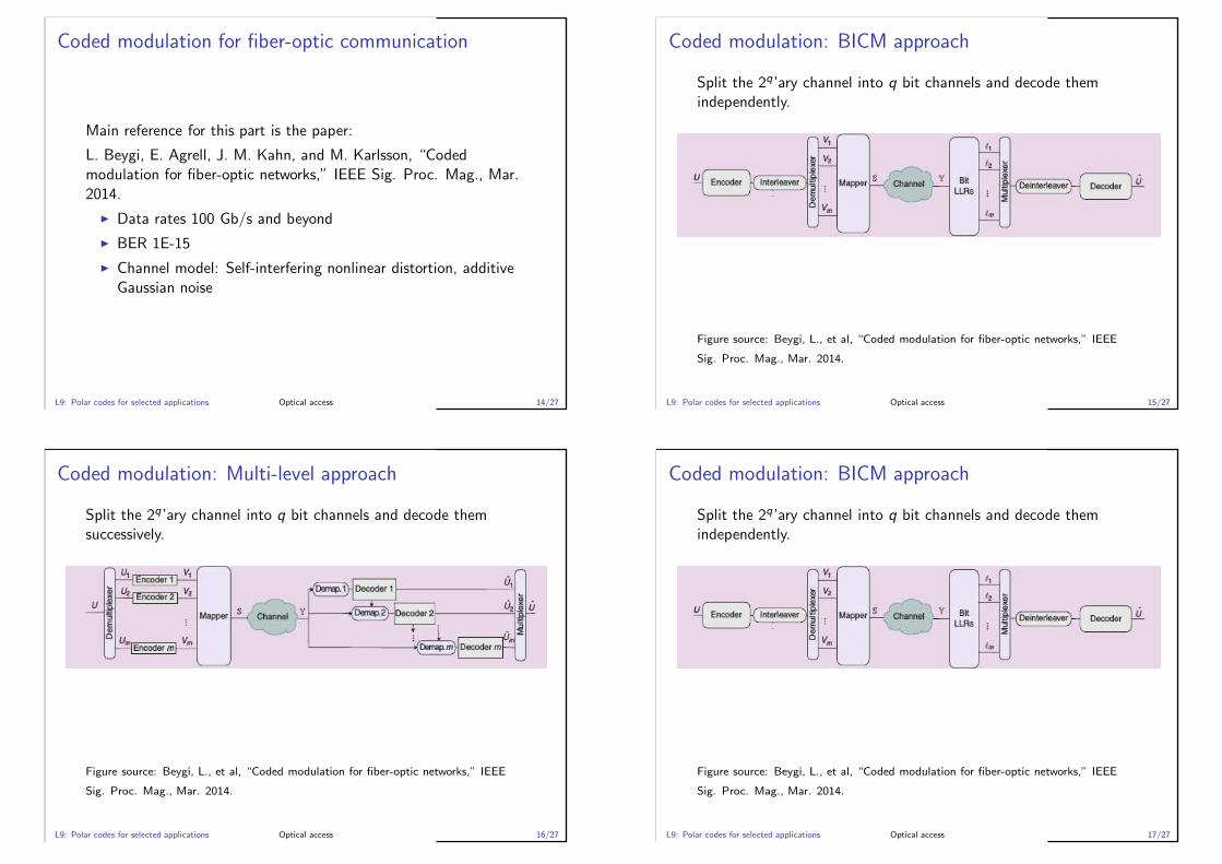
Coded modulation for fiber-optic communication
Main reference for this part is the paper:
L. Beygi, E. Agrell, J. M. Kahn, and M. Karlsson, “Codedmodulation for fiber-optic networks,” IEEE Sig. Proc. Mag., Mar.2014.
◮ Data rates 100 Gb/s and beyond
◮ BER 1E-15
◮ Channel model: Self-interfering nonlinear distortion, additiveGaussian noise
L9: Polar codes for selected applications Optical access 14/27
Coded modulation: BICM approach
Split the 2q ’ary channel into q bit channels and decode themindependently.
Figure source: Beygi, L., et al, “Coded modulation for fiber-optic networks,” IEEE
Sig. Proc. Mag., Mar. 2014.
L9: Polar codes for selected applications Optical access 15/27
Coded modulation: Multi-level approach
Split the 2q ’ary channel into q bit channels and decode themsuccessively.
Figure source: Beygi, L., et al, “Coded modulation for fiber-optic networks,” IEEE
Sig. Proc. Mag., Mar. 2014.
L9: Polar codes for selected applications Optical access 16/27
Coded modulation: BICM approach
Split the 2q ’ary channel into q bit channels and decode themindependently.
Figure source: Beygi, L., et al, “Coded modulation for fiber-optic networks,” IEEE
Sig. Proc. Mag., Mar. 2014.
L9: Polar codes for selected applications Optical access 17/27

Coded modulation: TCM approach
Split the 2q ’ary channels into two classes and encode the low-orderchannels using a trellis hand-crafted for large Euclidean distanceand ML-decoded
Figure source: Beygi, L., et al, “Coded modulation for fiber-optic networks,” IEEE
Sig. Proc. Mag., Mar. 2014.
L9: Polar codes for selected applications Optical access 18/27
Coded modulation: q’ary coding
No splitting; 2q ’ary processing applied; too complex
Figure source: Beygi, L., et al, “Coded modulation for fiber-optic networks,” IEEE
Sig. Proc. Mag., Mar. 2014.
L9: Polar codes for selected applications Optical access 19/27
Coded modulation: Polar approach
Split the 2q ’ary channel into “good”, “mediocre”, and “bad” bitchannels; apply coding only to mediocre channels
Figure source: Beygi, L., et al, “Coded modulation for fiber-optic networks,” IEEE
Sig. Proc. Mag., Mar. 2014.
L9: Polar codes for selected applications Optical access 20/27
Coded modulation: performance comparison
Figure source: Beygi, L., et al, “Coded modulation for fiber-optic networks,” IEEE
Sig. Proc. Mag., Mar. 2014.
L9: Polar codes for selected applications Optical access 21/27

Outline
◮ What is 5G?
◮ Technology proposals for 5G
◮ Polar coding for 5G
L9: Polar codes for selected applications 5G Scenarios 22/27
What is 5G?
Andrews et al.3 answer this question as follows.
◮ It willl not be an incremental advance over 4G.
◮ Will be characterized by
◮ Very high frequencies and massive bandwidths with very largeno of antennas
◮ Extreme base station and device connectivity
◮ Universal connectivity between 5G new air interfaces, LTE,WiFi, etc.
3Andrews et al., “What will 5G be?” JSAC 2014L9: Polar codes for selected applications 5G Scenarios 23/27
Technical requirements for 5G
Again, according to Andrews et al., 5G will have to meet thefollowing requirements (not all at once):
◮ Data rates compared to 4G
◮ Aggregate: 1000 times more capacity/km2 compared to 4G
◮ Cell-edge: 100 - 1000 Mb/s/user with 95% guarantee
◮ Peak: 10s of Gb/s/user
◮ Round-trip latency: Some applications (tactile Internet,two-way gaming, virtual reality) will require 1 ms latencycompared to 10-15 ms that 4G can provide
◮ Energy and cost: Link energy consumption should remain thesame as data rates increase, meaning that a 100-times moreenergy-efficient link is required
◮ No of devices: 10,000 more low-rate devices for M2Mcommunications, along with traditional high-rate users
L9: Polar codes for selected applications 5G Scenarios 24/27
Key technology ingredients for 5G
It is generally agreed that the 1000x aggregate data rate increasewill be possible through a combination of three types of gains.
◮ Densification of network access nodes
◮ Increased bandwidth (move to mm waves)
◮ Increased spectral efficiency through new communicationtechniques:
◮ advanced MIMO
◮ improved multi-access
◮ better interference management
◮ improved coding and modulation schemes
L9: Polar codes for selected applications 5G Scenarios 25/27

Summary
◮ With list-decoding and CRC polar codes deliver comparableperformance to LDPC and Turbo codes used in presentwireless standards
◮ SoA in coding is already close to theoretical limits forlow-order modulation, leaving little margin for improvement
◮ The biggest asset of polar coding compared to SoA is itsuniversal, flexible, and versatile nature
◮ Universal: the same hardware can be used with different codelengths, rates, channels
◮ Flexible: the code rate can be adjusted readily to any numberbetween 0 and 1
◮ Versatile: can be used in multi-terminal coding scenarios
L9: Polar codes for selected applications Polar code outlook 26/27
Outlook
◮ There is need for new FEC techniques as we move to 5Gscenarios that call for very high spectral efficiencies andadvanced multi-user and multi-antenna techniques
◮ Extensive research is needed before any FEC method can bedeclared a winner for 5G scenarios; the field is wide open forintroducing new techniques
◮ It is likely that the winner will emerge based on a trade-offbetween the overall communication performance under adiverse set of application scenarios and a number ofimplementation metrics such as complexity and energyefficiency
L9: Polar codes for selected applications Polar code outlook 27/27
Related Documents