A semismooth Newton method for SOCCPs based on a one-parametric class of SOC complementarity functions

A semismooth Newton method for SOCCPs based on aone-parametric class of SOC complementarity functions

Shaohua Pan 1

School of Mathematical Sciences

South China University of Technology

Guangzhou 510640, China

Jein-Shan Chen 2

Department of Mathematics

National Taiwan Normal University

Taipei 11677, Taiwan

March 26, 2007

(revised on July 30, 2007)

(2nd revised on October 28, 2007)

Abstract. In this paper, we present a detailed investigation for the properties of a one-

parametric class of SOC complementarity functions, which include the globally Lipschitz

continuity, strong semismoothness, and the characterization of the B-subdifferential at

a general point. Moreover, for the merit functions induced by them for the second-order

cone complementarity problem (SOCCP), we provide a condition for each stationary

point being a solution of the SOCCP and establish the boundedness of their level sets,

by exploiting Cartesian P -properties. We also propose a semismooth Newton method

based on the reformulation of the nonsmooth system of equations involving the class

of SOC complementarity functions. The global and superlinear convergence results are

obtained, and among others, the superlinear convergence is established under strict

complementarity. Preliminary numerical results are reported for DIMACS second-order

cone programs, which confirm the favorable theoretical properties of the method.

Key words. Second-order cone, complementarity, semismooth, B-subdifferential, New-

ton’s method.

1The author’s work is partially supported by the Doctoral Starting-up Foundation (B13B6050640)of GuangDong Province. E-mail:[email protected].

2Member of Mathematics Division, National Center for Theoretical Sciences, Taipei Office.The author’s work is partially supported by National Science Council of Taiwan. E-mail:[email protected].

1

1 Introduction

We consider the following conic complementarity problem of finding ζ ∈ IRn such that

F (ζ) ∈ K, G(ζ) ∈ K, 〈F (ζ), G(ζ)〉 = 0, (1)

where 〈·, ·〉 denotes the Euclidean inner product, F and G are the mappings from IRn to

IRn which are assumed to be continuously differentiable, and K is the Cartesian product

of second-order cones (SOCs), also called Lorentz cones [8]. In other words,

K = Kn1 ×Kn2 × · · · × Knm , (2)

where m,n1, . . . , nm ≥ 1, n1 + n2 + · · ·+ nm = n, and

Kni :={(x1, x2) ∈ IR× IRni−1 | x1 ≥ ‖x2‖

},

with ‖·‖ denoting the Euclidean norm and K1 denoting the set of nonnegative reals IR+.

We will refer to (1)–(2) as the second-order cone complementarity problem (SOCCP). In

addition, we write F = (F1, . . . , Fm) and G = (G1, . . . , Gm) with Fi, Gi : IRn → IRni .

An important special case of the SOCCP corresponds to G(ζ) = ζ for all ζ ∈ IRn.

Then (1) reduces to

F (ζ) ∈ K, ζ ∈ K, 〈F (ζ), ζ〉 = 0, (3)

which is a natural extension of the nonlinear complementarity problem (NCP) where

K = K1 × · · · × K1. Another important special case corresponds to the Karush-Kuhn-

Tucker (KKT) conditions of the convex second-order cone program (SOCP):

min g(x)

s.t. Ax = b, x ∈ K,(4)

where A ∈ IRm×n has full row rank, b ∈ IRm and g : IRn → IR is a twice continuously

differentiable convex function. From [7], the KKT conditions for (4), which are sufficient

but not necessary for optimality, can be written in the form of (1) with

F (ζ) := d + (I − AT (AAT )−1A)ζ, G(ζ) := ∇g(F (ζ))− AT (AAT )−1Aζ, (5)

where d ∈ IRn is any vector satisfying Ax = b. For large problems with a sparse A,

(5) has an advantage that the main cost of evaluating the Jacobian ∇F and ∇G lies in

inverting AAT , which can be done efficiently via sparse Cholesky factorization.

There have been various methods proposed for solving SOCPs and SOCCPs. They

include interior-point methods [1, 2, 17, 18, 24], non-interior smoothing Newton methods

[4, 9], the smoothing-regularization method [13], the merit function method [7] and the

semismooth Newton method [15]. Among others, the last four kinds of methods are all

2

based on an SOC complementarity function or a smooth merit function induced by it.

Given a mapping φ : IRl× IRl → IRl (l ≥ 1), we call φ an SOC complementarity function

associated with the cone Kl if for any (x, y) ∈ IRl × IRl,

φ(x, y) = 0 ⇐⇒ x ∈ Kl, y ∈ Kl, 〈x, y〉 = 0. (6)

Clearly, when l = 1, an SOC complementarity function reduces to an NCP function,

which plays an important role in the solution of NCPs; see [22] and references therein.

A popular choice of φ is the Fischer-Burmeister (FB) function [10, 11], defined by

φFB

(x, y) := (x2 + y2)1/2 − (x + y), (7)

where x2 means x◦x with “◦” denoting the Jordan product, and x+y denotes the usual

componentwise addition of vectors. More specifically, for any x = (x1, x2), y = (y1, y2) ∈IR× IRl−1, we define their Jordan product associated with Kl as

x ◦ y := (〈x, y〉, y1x2 + x1y2). (8)

The Jordan product, unlike scalar or matrix multiplication, is not associative, which

is the main source on complication in the analysis of SOCCPs. The identity element

under this product is e := (1, 0, · · · , 0)T ∈ IRl. It is known that x2 ∈ Kl for all x ∈ IRl.

Moreover, if x ∈ Kl, then there exists a unique vector in Kl, denoted by x1/2, such that

(x1/2)2 = x1/2 ◦ x1/2 = x. Thus, φFB

in (7) is well-defined for all (x, y) ∈ IRl × IRl. The

function φFB

was proved in [9] to satisfy the equivalence (6), and its squared norm

ψFB

(x, y) :=1

2‖φ

FB(x, y)‖2,

has been shown to be continuously differentiable everywhere by Chen and Tseng [7].

Another popular choice of φ is the residual function φNR : IRl × IRl → IRl given by

φNR(x, y) := x− [x− y]+,

where [ · ]+ means the minimum Euclidean distance projection onto Kl. The function

was studied in [9, 13] which is involved in smoothing methods for the SOCCP, and

recently it was used to develop a semismooth Newton method for nonlinear SOCPs by

Kanzow and Fukushima [15]. The function φNR also induces a merit function

ψNR(x, y) :=1

2‖φNR(x, y)‖2,

but, compared to ψFB

, it has a remarkable drawback, i.e. the non-differentiability.

In this paper, we consider a one-parametric class of vector-valued functions

φτ (x, y) :=[(x− y)2 + τ(x ◦ y)

]1/2 − (x + y) (9)

3

with τ being an arbitrary fixed parameter from (0, 4). The class of functions is a natural

extension of the family of NCP functions proposed by Kanzow and Kleinmichel [14], and

has been shown to satisfy the characterization (6) in [6]. It is not hard to see that as

τ = 2, φτ reduces to the FB function φFB

in (7) while it becomes a multiple of the natural

residual function φNR as τ → 0+. With the class of SOC complementarity functions, the

SOCCP can be reformulated as a nonsmooth system of equations

Φτ (ζ) :=

φτ (F1(ζ), G1(ζ))...

φτ (Fi(ζ), Gi(ζ))...

φτ (Fm(ζ), Gm(ζ))

= 0, (10)

which induces a natural merit function Ψτ : IRn → IR+ given by

Ψτ (ζ) =1

2‖Φτ (ζ)‖2 =

m∑i=1

ψτ (Fi(ζ), Gi(ζ), (11)

with

ψτ (x, y) =1

2‖φτ (x, y)‖2. (12)

In [6], we studied the continuous differentiability of ψτ and proved that each stationary

point of Ψτ is a solution of the SOCCP if ∇F and −∇G are column monotone. This

paper focuses on other properties of φτ , including the globally Lipschitz continuity, the

strong semismoothness, and the characterization of the B-subdifferential. Particularly,

we provide a weaker condition than [6] for each stationary point of Ψτ to be a solution

of the SOCCP and establish the boundedness of the level sets of Ψτ , by using Cartesian

P -properties. We also propose a semismooth Newton method based on (10), and obtain

the corresponding global and the superlinear convergence results. Among others, the

superlinear convergence is established under strict complementarity.

Throughout this paper, I represents an identity matrix of suitable dimension, and

IRn1×· · ·×IRnm is identified with IRn1+···+nm . For a differentiable mapping F : IRn → IRm,

∇F (x) denotes the transpose of the Jacobian F ′(x). For a symmetric matrix A ∈ IRn×n,

we write A º O (respectively, A Â O) to mean A is positive semidefinite (respectively,

positive definite). Given a finite number of square matrices Q1, . . . , Qm, we denote the

block diagonal matrix with these matrices as block diagonals by diag(Q1, . . . , Qm) or by

diag(Qi, i = 1, . . . , m). If J and B are index sets such that J ,B ⊆ {1, 2, . . . , m}, we

denote PJB by the block matrix consisting of the submatrices Pjk ∈ IRnj×nk of P with

j ∈ J , k ∈ B, and by xB a vector consisting of subvectors xi ∈ IRni with i ∈ B.

4

2 Preliminaries

This section recalls some background materials and preliminary results that will be used

in the subsequent sections. We begin with the interior and the boundary of Kl (l ≥ 1).

It is known that Kl is a closed convex self-dual cone with nonempty interior given by

int(Kl) :={x = (x1, x2) ∈ IR× IRl−1 | x1 > ‖x2‖

}

and the boundary given by

bd(Kl) :={x = (x1, x2) ∈ IR× IRl−1 | x1 = ‖x2‖

}.

For each x = (x1, x2) ∈ IR× IRl−1, the determinant and the trace of x are defined by

det(x) := x21 − ‖x2‖2, tr(x) := 2x1.

In general, det(x ◦ y) 6= det(x) det(y) unless x2 = αy2 for some α ∈ IR. A vector x ∈ IRl

is said to be invertible if det(x) 6= 0, and its inverse is denoted by x−1. Given a vector

x = (x1, x2) ∈ IR× IRl−1, we often use the following symmetry matrix

Lx :=

[x1 xT

2

x2 x1I

], (13)

which can be viewed as a linear mapping from IRl to IRl. It is easy to verify Lxy = x ◦ y

and Lx+y = Lx + Ly for any x, y ∈ IRl. Furthermore, x ∈ Kl if and only if Lx º O, and

x ∈ int(Kl) if and only if Lx  O. If x ∈ int(Kl), then Lx is invertible with

L−1x =

1

det(x)

x1 −xT2

−x2det(x)

x1

I +1

x1

x2xT2

. (14)

We recall from [9] that each x = (x1, x2) ∈ IR× IRl−1 admits a spectral factorization,

associated with Kl, of the form

x = λ1(x) · u(1)x + λ2(x) · u(2)

x ,

where λi(x) and u(i)x for i = 1, 2 are the spectral values and the associated spectral

vectors of x, respectively, given by

λi(x) = x1 + (−1)i‖x2‖, u(i)x =

1

2

(1, (−1)ix2

)(15)

with x2 = x2/‖x2‖ if x2 6= 0, and otherwise x2 being any vector in IRl−1 such that

‖x2‖ = 1. If x2 6= 0, then the factorization is unique. The spectral decomposition of

x, x2 and x1/2 has some basic properties as below, whose proofs can be found in [9].

5

Property 2.1 For any x = (x1, x2) ∈ IR × IRl−1 with the spectral values λ1(x), λ2(x)

and spectral vectors u(1)x , u

(2)x given as above, the following results hold:

(a) x ∈ Kl if and only if λ1(x) ≥ 0, and x ∈ int(Kl) if and only if λ1(x) > 0.

(b) x2 = λ21(x)u

(1)x + λ2

2(x)u(2)x ∈ Kl;

(c) x1/2 =√

λ1(x) u(1)x +

√λ2(x) u

(2)x ∈ Kl if x ∈ Kl.

(d) det(x) = λ1(x)λ2(x), tr(x) = λ1(x) + λ2(x) and ‖x‖2 = [λ21(x) + λ2

2(x)]/2.

For the sake of notation, throughout the rest of this paper, we always write

w = (w1, w2) = w(x, y) := (x− y)2 + τ(x ◦ y),

z = (z1, z2) = z(x, y) :=[(x− y)2 + τ(x ◦ y)

]1/2(16)

for any x = (x1, x2), y = (y1, y2) ∈ IR × IRl−1, and let w2 = w2/‖w2‖ if w2 6= 0, and

otherwise w2 be any vector in IRl−1 satisfying ‖w2‖ = 1. We have

w1 = ‖x‖2 + ‖y‖2 + (τ − 2)xT y, w2 = 2(x1x2 + y1y2) + (τ − 2)(x1y2 + y1x2).

Moreover, w ∈ Kl and z ∈ Kl hold by noting that

w = x2 + y2 + (τ − 2)(x ◦ y) =

(x +

τ − 2

2y

)2

+τ(4− τ)

4y2

=

(y +

τ − 2

2x

)2

+τ(4− τ)

4x2. (17)

In addition, using Property 2.1 (b) and (c), it is not hard to compute that

z =

(√λ2(w) +

√λ1(w)

2,

√λ2(w)−

√λ1(w)

2w2

)∈ Kl. (18)

The following lemma characterizes the set of points where z(x, y) is (continuously)

differentiable. Since the proof is direct by the arguments in Case (2) of [6, Proposition

3.2] and formulas (18) and (14), we here omit it.

Lemma 2.1 The function z(x, y) defined by (16) is (continuously) differentiable at a

point (x, y) if and only if (x− y)2 + τ(x ◦ y) ∈ int(Kl), and furthermore,

∇xz(x, y) = Lx+ τ−22

yL−1z , ∇yz(x, y) = Ly+ τ−2

2xL

−1z ,

where

L−1z =

(b cwT

2

cw2 aI + (b− a)w2wT2

)if w2 6= 0;

(1/√

w1

)I if w2 = 0,

(19)

with a = 2√λ2(w)+

√λ1(w)

, b = 12

(1√

λ2(w)+ 1√

λ1(w)

)and c = 1

2

(1√

λ2(w)− 1√

λ1(w)

).

6

Lemma 2.2 [6, Lemma 3.1] For any x = (x1, x2), y = (y1, y2) ∈ IR × IRl−1, let

w = (w1, w2) be given as in (16). If (x− y)2 + τ(x ◦ y) /∈ int(Kl), then

x21 = ‖x2‖2, y2

1 = ‖y2‖2, x1y1 = xT2 y2, x1y2 = y1x2; (20)

x21 + y2

1 + (τ − 2)x1y1 = ‖x1x2 + y1y2 + (τ − 2)x1y2‖= ‖x2‖2 + ‖y2‖2 + (τ − 2)xT

2 y2. (21)

If, in addition, (x, y) 6= (0, 0), then w2 6= 0, and moreover,

xT2 w2 = x1, x1w2 = x2, yT

2 w2 = y1, y1w2 = y2. (22)

Lemma 2.3 [6, Lemma 3.2] For any x = (x1, x2), y = (y1, y2) ∈ IR × IRl−1, let w =

(w1, w2) be defined as in (16). If w2 6= 0, then for i = 1, 2,

[(x1 +

τ − 2

2y1

)+ (−1)i

(x2 +

τ − 2

2y2

)T

w2

]2

≤∥∥∥∥(

x2 +τ − 2

2y2

)+ (−1)i

(x1 +

τ − 2

2y1

)w2

∥∥∥∥2

≤ λi(w).

Furthermore, these relations also hold when interchanging x and y.

To close this section, we recall some concepts that will be used in the sequel. Given

a mapping H : IRn → IRm, if H is locally Lipschitz continuous, the following set

∂BH(z) :={V ∈ IRm×n| ∃{zk} ⊆ DH : zk → z,H ′(zk) → V

}

is nonempty and is called the B-subdifferential of H at z, where DH ⊆ IRn denotes the

set of points at which H is differentiable. The convex hull ∂H(z) := conv∂BH(z) is the

generalized Jacobian of H at z in the sense of Clarke [5]. For the concepts of (strongly)

semismooth functions, please refer to [20, 21] for details. We next present definitions of

Cartesian P -properties for a matrix M ∈ IRn×n, which are in fact special cases of those

introduced by Chen and Qi [3] for a linear transformation.

Definition 2.1 A matrix M ∈ IRn×n is said to have

(a) the Cartesian P -property if for any 0 6= x = (x1, . . . , xm) ∈ IRn with xi ∈ IRni, there

exists an index ν ∈ {1, 2, . . . , m} such that 〈xν , (Mx)ν〉 > 0;

(b) the Cartesian P0-property if for any 0 6= x = (x1, . . . , xm) ∈ IRn with xi ∈ IRni,

there exists an index ν ∈ {1, 2, . . . ,m} such that xν 6= 0 and 〈xν , (Mx)ν〉 ≥ 0.

Some nonlinear generalizations of these concepts in the setting ofK are defined as follows.

7

Definition 2.2 Given a mapping F = (F1, . . . , Fm) with Fi : IRn → IRni, F is said to

(a) have the uniform Cartesian P -property if for any x = (x1, . . . , xm), y = (y1, . . . , ym) ∈IRn, there is an index ν ∈ {1, 2, . . . , m} and a constant ρ > 0 such that

〈xν − yν , Fν(x)− Fν(y)〉 ≥ ρ‖x− y‖2;

(b) have the Cartesian P0-property if for any x = (x1, . . . , xm), y = (y1, . . . , ym) ∈ IRn

and x 6= y, there exists an index ν ∈ {1, 2, . . . , m} such that

xν 6= yν and 〈xν − yν , Fν(x)− Fν(y)〉 ≥ 0.

3 Properties of the functions φτ and Φτ

First, we study the favorable properties of φτ , including the globally Lipschitz continuity,

the strong semismoothness and the characterization of the B-subdifferential at any point.

Proposition 3.1 The function φτ defined as in (9) has the following properties.

(a) φτ is (continuously) differentiable at (x, y) if and only if w(x, y) ∈ int(Kl). Also,

∇xφτ (x, y) = Lx+ τ−22

yL−1z − I, ∇yφτ (x, y) = Ly+ τ−2

2xL

−1z − I.

(b) φτ is globally Lipschitz continuous with the Lipschitz constant independent of τ .

(c) φτ is strongly semismooth at any (x, y) ∈ IRl × IRl.

(d) The squared norm of φτ , i.e. ψτ , is continuously differentiable everywhere.

Proof. (a) The proof directly follows from Lemma 2.1 and the following fact that

φτ (x, y) = z(x, y)− (x + y). (23)

(b) It suffices to prove that z(x, y) is globally Lipschitz continuous by (23). Let

z = z(x, y, ε) :=[(x− y)2 + τ(x ◦ y) + εe

]1/2(24)

for any ε > 0 and x = (x1, x2), y = (y1, y2) ∈ IR× IRl−1. Then, applying Lemma A.1 in

the appendix and the Mean-Value Theorem, we have∥∥∥z(x, y)− z(a, b)

∥∥∥ =

∥∥∥∥ limε→0+

z(x, y, ε)− limε→0+

z(a, b, ε)

∥∥∥∥≤ lim

ε→0+‖z(x, y, ε)− z(a, y, ε) + z(a, y, ε)− z(a, b, ε)‖

≤ limε→0+

∥∥∥∥∫ 1

0

∇xz(a + t(x− a), y, ε)(x− a)dt

∥∥∥∥

+ limε→0+

∥∥∥∥∫ 1

0

∇yz(a, b + t(y − b), ε)(y − b)dt

∥∥∥∥≤

√2C‖(x, y)− (a, b)‖

8

for any (x, y), (a, b) ∈ IRl × IRl, where C > 0 is a constant independent of τ .

(c) From the definition of φτ and φFB

, it is not hard to check that

φτ (x, y) = φFB

(x +

τ − 2

2y,

√τ(4− τ)

2y

)+

1

2

(τ − 4 +

√τ(4− τ)

)y.

Notice that φFB

is strongly semismooth by [23, Corollary 3.3], and the functions x+ τ−22

y,12

√τ(4− τ)y and 1

2(τ − 4+

√τ(4− τ))y are also strongly semismooth. Therefore, φτ is

a strongly semismooth function since by [11, Theorem 19] the composition of strongly

semismooth functions is strongly semismooth.

(d) The proof can be found in Proposition 3.3 of [6]. 2

Proposition 3.1 (c) indicates that, when a smoothing or nonsmooth Newton method is

used to solve system (10), a fast convergence rate (at least superlinear) may be expected.

To develop a semismooth Newton method for the SOCCP, we need to characterize the

B-subdifferential ∂Bφτ (x, y) at a general point (x, y). The discussion of B-subdifferential

for φFB

was given in [19], and we here generalize it to φτ for any τ ∈ (0, 4). The detailed

derivation process is included in the appendix for completeness.

Proposition 3.2 Given a general point (x, y) ∈ IR× IRl−1, each element in ∂Bφτ (x, y)

is of the form V = [Vx − I Vy − I] with Vx and Vy having the following representation:

(a) If (x− y)2 + τ(x ◦ y) ∈ int(Kl), then Vx = L−1z Lx+ τ−2

2y and Vy = L−1

z Ly+ τ−22

x.

(b) If (x− y)2 + τ(x ◦ y) ∈ bd(Kl) and (x, y) 6= (0, 0), then

Vx ∈{

1

2√

2w1

(1 wT

2

w2 4I − 3w2wT2

)(Lx +

τ − 2

2Ly

)+

1

2

(1

−w2

)uT

}

Vy ∈{

1

2√

2w1

(1 wT

2

w2 4I − 3w2wT2

)(Ly +

τ − 2

2Lx

)+

1

2

(1

−w2

)vT

}(25)

for some u = (u1, u2), v = (v1, v2) ∈ IR × IRl−1 satisfying |u1| ≤ ‖u2‖ ≤ 1 and

|v1| ≤ ‖v2‖ ≤ 1, where w2 = w2

‖w2‖ .

(c) If (x, y) = (0, 0), then Vx ∈ {Lu}, Vy ∈ {Lv} for some u = (u1, u2), v = (v1, v2) ∈IR× IRl−1 satisfying ‖u‖, ‖v‖ ≤ 1 and u1v2 + v1u2 = 0, or

Vx ∈{

1

2

(1

w2

)ξT +

1

2

(1

−w2

)uT + 2

(0 0

(I − w2wT2 )s2 (I − w2w

T2 )s1

)}

Vy ∈{

1

2

(1

w2

)ηT +

1

2

(1

−w2

)vT + 2

(0 0

(I − w2wT2 )ω2 (I − w2w

T2 )ω1

)}(26)

9

for some u = (u1, u2), v = (v1, v2), ξ = (ξ1, ξ2), η = (η1, η2) ∈ IR × IRl−1 satisfying

|u1| ≤ ‖u2‖ ≤ 1, |v1| ≤ ‖v2‖ ≤ 1, |ξ1| ≤ ‖ξ2‖ ≤ 1 and |η1| ≤ ‖η2‖ ≤ 1,

w2 ∈ IRl−1 satisfying ‖w2‖ = 1, and s = (s1, s2), ω = (ω1, ω2) ∈ IR × IRl−1 such

that ‖s‖2 + ‖ω‖2 ≤ 1.

In what follows, we investigate the properties of the operator Φτ : IRn → IRn given

by (10). We start with the semismoothness of Φτ . Since Φτ is (strongly) semismooth if

and only if all component functions are (strongly) semismooth, and since the composite

of (strongly) semismooth functions is (strongly) semismooth by [11, Theorem 19], we

obtain the following conclusion as an immediate consequence of Proposition 3.1 (c).

Proposition 3.3 The operator Φτ : IRn → IRn given by (10) is semismooth. Moreover,

it is strongly semismooth if F ′ and G′ are locally Lipschitz continuous.

To characterize the B-subdifferential of Φτ , we write Fi(ζ) = (Fi1(ζ), Fi2(ζ)) and

Gi(ζ) = (Gi1(ζ), Gi2(ζ)), and denote wi and zi for i = 1, 2, . . . , m by

wi = (wi1(ζ), wi2(ζ)) = w(Fi(ζ), Gi(ζ)), zi = (zi1(ζ), zi2(ζ)) = z(Fi(ζ), Gi(ζ)). (27)

For convenience, we sometimes suppress in Fi(ζ) and Gi(ζ) the dependence on ζ.

Proposition 3.4 Let Φτ : IRn → IRn be defined as in (10). Then, for any ζ ∈ IRn,

∂BΦτ (ζ)T ⊆ ∇F (ζ) (A(ζ)− I) +∇G(ζ) (B(ζ)− I) , (28)

where A(ζ) and B(ζ) are possibly multivalued n × n block diagonal matrices whose ith

blocks Ai(ζ) and Bi(ζ) for i = 1, 2, . . . , m have the following representation.

(a) If (Fi(ζ)−Gi(ζ))2 + τ (Fi(ζ) ◦Gi(ζ)) ∈ int(Kni), then

Ai(ζ) = LFi+τ−22

GiL−1

ziand Bi(ζ) = LGi+

τ−22

FiL−1

zi.

(b) If (Fi(ζ), Gi(ζ)) 6= (0, 0) and (Fi(ζ)−Gi(ζ))2 + τ (Fi(ζ) ◦Gi(ζ)) ∈ bd(Kni), then

Ai(ζ) ∈{

1

2√

2wi1

(LFi

+τ − 2

2LGi

)(1 wT

i2

wi2 4I − 3wi2wTi2

)+

1

2ui(1,−wT

i2)

}

Bi(ζ) ∈{

1

2√

2wi1

(LGi

+τ − 2

2LFi

)(1 wT

i2

wi2 4I − 3wi2wTi2

)+

1

2vi(1,−wT

i2)

}

for some ui = (ui1, ui2), vi = (vi1, vi2) ∈ IR × IRni−1 satisfying |ui1| ≤ ‖ui2‖ ≤ 1

and |vi1| ≤ ‖vi2‖ ≤ 1, where wi2 = wi2

‖wi2‖ .

10

(c) If (Fi(ζ), Gi(ζ)) = (0, 0), then

Ai(ζ) ∈{

Lui

}∪

{1

2ξi

(1, wT

i2

)+

1

2ui

(1,−wT

i2

)+

(0 2sT

i2(I − wi2wTi2)

0 2si1(I − wi2wTi2)

)}

Bi(ζ) ∈{

Lvi

}∪

{1

2ηi

(1, wT

i2

)+

1

2vi

(1,−wT

i2

)+

(0 2ωT

i2(I − wi2wTi2)

0 2ωi1(I − wi2wTi2)

)}

for some ui = (ui1, ui2), vi = (vi1, vi2) ∈ IR × IRni−1 satisfying ‖ui‖, ‖vi‖ ≤ 1

and ui1vi2 + vi1ui2 = 0, some ui = (ui1, ui2), vi = (vi1, vi2), ξi = (ξi1, ξi2), ηi =

(ηi1, ηi2) ∈ IR × IRni−1 with |ui1| ≤ ‖ui2‖ ≤ 1, |vi1| ≤ ‖vi2‖ ≤ 1, |ξi1| ≤ ‖ξi2‖ ≤ 1

and |ηi1| ≤ ‖ηi2‖ ≤ 1, wi2 ∈ IRni−1 satisfying ‖wi2‖ = 1, and si = (si1, si2), ωi =

(ωi1, ωi2) ∈ IR× IRni−1 such that ‖si‖2 + ‖ωi‖2 ≤ 1.

Proof. Let Φτ,i(ζ) denote the ith subvector of Φτ , i.e. Φτ,i(ζ) = φτ (Fi(ζ), Gi(ζ)) for all

i = 1, 2, . . . , m. From Proposition 2.6.2 of [5], it follows that

∂BΦτ (ζ)T ⊆ ∂BΦτ,1(ζ)T × ∂BΦτ,2(ζ)T × · · · × ∂BΦτ,m(ζ)T , (29)

where the latter denotes the set of all matrices whose (ni−1 + 1) to nith columns with

n0 = 0 belong to ∂BΦτ,i(ζ)T . Using the definition of B-subdifferential and the continuous

differentiability of F and G, it is not difficult to verify that

∂BΦτ,i(ζ)T = [∇Fi(ζ) ∇Gi(ζ)]∂Bφτ (Fi(ζ), Gi(ζ))T , i = 1, . . . , m. (30)

Using Proposition 3.2 and the last two equations, we readily get the desired result. 2

Lemma 3.1 For any ζ ∈ IRn, let A(ζ) and B(ζ) be the multivalued block diagonal

matrices given as in Proposition 3.4. Then, for any i ∈ {1, 2, . . . , m},

〈(Ai(ζ)− I)Φτ,i(ζ), (Bi(ζ)− I)Φτ,i(ζ)〉 ≥ 0,

and the equality holds if and only if Φτ,i(ζ) = 0. Particularly, for the index i such that

(Fi(ζ)−Gi(ζ))2 + τ(Fi(ζ) ◦Gi(ζ) ∈ int(Kni), we have

〈(Ai(ζ)− I)υi, (Bi(ζ)− I)υi〉 ≥ 0, for any υi ∈ IRni .

Proof. From Theorem 2.6.6 of [5] and Proposition 3.1 (d), we have

∇ψτ (x, y) = ∂Bφτ (x, y)T φτ (x, y).

Consequently, for any i = 1, 2, . . . , m, it follows that

∇ψτ (Fi(ζ), Gi(ζ)) = ∂Bφτ (Fi(ζ), Gi(ζ))T φτ (Fi(ζ), Gi(ζ)).

11

In addition, from Propositions 3.2 and 3.4, it is not hard to see that

[Ai(ζ)T − I Bi(ζ)T − I] ∈ ∂Bφτ (Fi(ζ), Gi(ζ)).

Combining with the last two equations yields that for any i = 1, 2, . . . ,m,

∇xψτ (Fi(ζ), Gi(ζ)) = (Ai(ζ)− I)Φτ,i(ζ)

∇yψτ (Fi(ζ), Gi(ζ)) = (Bi(ζ)− I)Φτ,i(ζ). (31)

Consequently, the first part of the conclusions is direct by Proposition 4.1 of [6]. Notice

that for any i such that (Fi(ζ)−Gi(ζ))2 + τ(Fi(ζ) ◦Gi(ζ) ∈ int(Kni) and any υi ∈ IRni ,

〈(Ai(ζ)− I)υi, (Bi(ζ)− I)υi〉=

⟨(LFi+

τ−22

Gi− Lzi

)L−1

ziυi,

(LGi+

τ−22

Fi− Lzi

)L−1

ziυi

⟩

=⟨(

LGi+τ−22

Fi− Lzi

)(LFi+

τ−22

Gi− Lzi

)L−1

ziυi, L−1

ziυi

⟩. (32)

Therefore, using the same argument as Case (2) of [6, Proposition 4.1], we can obtain

the second part of the conclusions. 2

4 Nonsingularity conditions

In this section, we show that all elements of the B-subdifferential ∂BΦτ (ζ) at a solution

ζ∗ of the SOCCP are nonsingular if ζ∗ satisfies strict complementarity, i.e.,

Fi(ζ∗) + Gi(ζ

∗) ∈ int(Kni) for all i = 1, 2, . . . ,m. (33)

First, we give a technical lemma which states that the multivalued matrix (Ai(ζ∗)−I)+

(Bi(ζ∗)− I) are nonsingular if the ith block component satisfies strict complementarity.

Lemma 4.1 Let ζ∗ be a solution of the SOCCP, and A(ζ∗) and B(ζ∗) be the multivalued

block diagonal matrices characterized by Proposition 3.4. Then, for any i ∈ {1, 2, . . . , m}such that Fi(ζ

∗) + Gi(ζ∗) ∈ int(Kni), we have that Φτ,i(ζ) is continuously differentiable

at ζ∗ and (Ai(ζ∗)− I) + (Bi(ζ

∗)− I) is nonsingular.

Proof. Since ζ∗ is a solution of the SOCCP, we have for all i = 1, 2, . . . , m

Fi(ζ∗) ∈ Kni , Gi(ζ

∗) ∈ Kni , 〈Fi(ζ∗), Gi(ζ

∗)〉 = 0.

It is not hard to verify that Fi(ζ∗) + Gi(ζ

∗) ∈ int(Kni) if and only if one of the three

cases shown as below holds.

12

Case (1). Fi(ζ∗) ∈ int(Kni) and Gi(ζ

∗) = 0. Under this case,

wi(ζ∗) = (Fi(ζ

∗)−Gi(ζ∗))2 + τ(Fi(ζ

∗) ◦Gi(ζ∗)) = Fi(ζ

∗)2 ∈ int(Kni).

By Proposition 3.1 (a), Φτ,i(ζ) is continuously differentiable at ζ∗. Since zi(ζ∗) =

wi(ζ∗)1/2 = Fi(ζ

∗), from Proposition 3.4 (a) it follows that

Ai(ζ∗) = I and Bi(ζ

∗) =τ − 2

2I,

which implies that (Ai(ζ∗)− I) + (Bi(ζ

∗)− I) is nonsingular since 0 < τ < 4.

Case (2). Fi(ζ∗) = 0 and Gi(ζ

∗) ∈ int(Kni). Now, wi(ζ∗) = Gi(ζ

∗)2 ∈ int(Kni). So,

Φτ,i(ζ) is continuously differentiable at ζ∗ by Proposition 3.1 (a). Since

zi(ζ∗) = wi(ζ

∗)1/2 = Gi(ζ∗),

using Proposition 3.4 (a) yields that Ai(ζ∗) = τ−2

2I and Bi(ζ

∗) = I, which immediately

implies that (Ai(ζ∗)− I) + (Bi(ζ

∗)− I) is nonsingular.

Case (3). Fi(ζ∗) ∈ bd+(Kni) and Gi(ζ

∗) ∈ bd+(Kni). We claim that wi(ζ∗) ∈ int(Kni)

for this case. If not, then wi(ζ∗) ∈ bd(Kni). From (20) in Lemma 2.2, it follows that

Fi1(ζ∗)Gi1(ζ

∗) = Fi2(ζ∗)T Gi2(ζ

∗). (34)

Since Fi1(ζ∗) = ‖Fi2(ζ

∗)‖ 6= 0 and Gi1(ζ∗) = ‖Gi2(ζ

∗)‖ 6= 0, we have

‖Fi2(ζ∗)‖ · ‖Gi2(ζ

∗)‖ = Fi2(ζ∗)T Gi2(ζ

∗),

which implies that Fi2(ζ∗) = αGi2(ζ

∗) for some constant α > 0. Substituting it into

(34) yields that Fi1(ζ∗) = αGi1(ζ

∗), and consequently, Fi(ζ∗) = αGi(ζ

∗). Noting that

〈Fi(ζ∗), Gi(ζ

∗)〉 = 0, we then obtain Fi(ζ∗) = Gi(ζ

∗) = 0. This clearly contradicts the

assumption that Fi(ζ∗) 6= 0 and Gi(ζ

∗) 6= 0. Hence, wi(ζ∗) ∈ int(Kni).

From the expression of Ai(ζ) and Bi(ζ) given by Proposition 3.4 (a),

(Ai(ζ∗)− I) + (Bi(ζ

∗)− I) = −L2zi(ζ∗)− τ2(Fi(ζ∗)+Gi(ζ∗))L

−1zi(ζ∗).

Therefore, to establish the nonsingularity of (Ai(ζ∗) − I) + (Bi(ζ

∗) − I), it suffices to

prove that the matrix L2zi(ζ∗)− τ2(Fi(ζ∗)+Gi(ζ∗)) is nonsingular. Since

(2zi(ζ

∗))2

= 2

[(Fi(ζ

∗) +τ − 2

2Gi(ζ

∗))2

+τ(4− τ)

4Gi(ζ

∗)2

]

+2

[(Gi(ζ

∗) +τ − 2

2Fi(ζ

∗))2

+τ(4− τ)

4Fi(ζ

∗)2

],

13

it follows that

(2zi(ζ

∗))2

− τ 2

4

(Fi(ζ

∗) + Gi(ζ∗)

)2

=τ(4− τ)

2

[Gi(ζ

∗)2 + Fi(ζ∗)2

]

+(4− τ)2

4

(Fi(ζ

∗)−Gi(ζ∗)

)2

. (35)

Notice that wi(ζ∗) ∈ int(Kni) implies that (Fi(ζ

∗) − Gi(ζ∗))2 ∈ int(Kni) since Fi(ζ

∗) ◦Gi(ζ

∗) = 0, and hence from the equality (35) we immediately obtain that

(2zi(ζ

∗))2

− τ 2

4

(Fi(ζ

∗) + Gi(ζ∗)

)2

∈ int(Kni).

Since zi(ζ∗) = wi(ζ

∗)1/2 ∈ int(Kni), using Proposition 3.4 of [9] yields that

2zi(ζ∗)− τ

2(Fi(ζ

∗) + Gi(ζ∗)) ∈ int(Kni).

This means that L2zi(ζ∗)− τ2(Fi(ζ∗)+Gi(ζ∗)) Â O, and consequently it is nonsingular. 2

Given a solution ζ∗ of the SOCCP, we know from [1] that, if ζ∗ is a strict comple-

mentarity one, i.e. satisfies the conditions in (33), the following index sets

I :={

i ∈ {1, 2, . . . , m} | Fi(ζ∗) ∈ int(Kni), Gi(ζ

∗) = 0}

,

B :={

i ∈ {1, 2, . . . , m} | Fi(ζ∗) ∈ bd+(Kni), Gi(ζ

∗) ∈ bd+(Kni)}

, (36)

J :={

i ∈ {1, 2, . . . , m}| Fi(ζ∗) = 0, Gi(ζ

∗) ∈ int(Kni)}

form a partition of {1, . . . , m}, where bd+(Kni) = bd(Kni) \{0}. Thus, by supposing

that ∇G(ζ∗) is invertible and rearranging the matrices appropriately,

P (ζ∗) = ∇G(ζ∗)−1∇F (ζ∗) =

P (ζ∗)II P (ζ∗)IB P (ζ∗)IJP (ζ∗)BI P (ζ∗)BB P (ζ∗)BJP (ζ∗)JI P (ζ∗)JB P (ζ∗)JJ

.

Now we are in a position to establish the nonsingularity of all elements in ∂BΦτ (ζ∗).

Theorem 4.1 Let ζ∗ be a strict complementarity solution of the SOCCP. Suppose that

∇G(ζ∗) is invertible and let P (ζ∗) = ∇G(ζ∗)−1∇F (ζ∗). If P (ζ∗)JJ is nonsingular and

its Schur-complement, denoted by P (ζ∗)JJ , in the matrix

(P (ζ∗)BB P (ζ∗)BJP (ζ∗)JB P (ζ∗)JJ

)

has the Cartesian P -property, then all W ∈ ∂BΦτ (ζ∗) are nonsingular.

14

Proof. By Proposition 3.4 and the invertibility of ∇G(ζ∗), it suffices to show that any

matrix C belonging to ∇G(ζ∗)−1∇F (ζ∗)(A(ζ∗)− I)+ (B(ζ∗)− I) is invertible. Since ζ∗

is a strict complementarity solution, it follows from Lemma 4.1 that the matrix C can

be written in the following partitioned form

C =

τ − 4

2II PIB(AB − IB)

τ − 4

2PIJ

0BI PBB(AB − IB) + (BB − IB)τ − 4

2PBJ

0JI PJB(AB − IB)τ − 4

2PJJ

,

where II = diag(Ii, i ∈ I) with Ii being an ni×ni identity matrix, AB = diag(Ai, i ∈ B)

and BB = diag(Bi, i ∈ B). For the sake of notation, we here omit the notation ζ∗ in

the functions. It is not hard to see that these C are nonsingular if and only if

Cr =

PBB(AB − IBB) + (BB − IBB)τ − 4

2PBJ

PJB(AB − IBB)τ − 4

2PJJ

is nonsingular. Showing that Cr is nonsingular is equivalent to showing that the system

−Cr

(yByJ

)= 0

for any y = (yB; yJ ) has only the zero solution. This system can be rewritten as

4− τ

2PJJ yJ + PJB(IBB − AB)yB = 0,

4− τ

2PBJ yJ + PBB(IBB − AB)yB = −(IBB −BB)yB.

Recall that PJJ is nonsingular, and we obtain from the last system that

yJ = − 2

4− τP−1JJPJB(IBB − AB)yB,

(PBB − PBJP−1JJPJB)(IBB − AB)yB = −(IBB −BB)yB.

(37)

Thus, by Lemma 3.1 and Lemma 4.1, using the same arguments as Theorem 4.1 of [19]

yields the desired result. 2

Observe that, when n1 = · · · = nm = 1, the assumption for PJJ is actually equiv-

alent to requiring that PJJ is a P -matrix, which is common in the solution of NCPs.

Now, we are not clear whether the result of Theorem 4.1 holds when removing the strict

complementarity. We will leave it as a future research topic.

From Theorem 4.1 and [21, Lemma 2.6], we readily obtain the following result.

15

Corollary 4.1 Suppose that ζ∗ is a strict complementarity solution of the SOCCP and

the mapping F and G at the ζ∗ satisfy the conditions of Theorem 4.1. Then, there exist

a neighborhood N (ζ∗) of ζ∗ and a constant C > 0 such that for any ζ ∈ N (ζ∗) and any

W ∈ ∂BΦτ (ζ), W is nonsingular and satisfies ‖W−1‖ ≤ C.

5 Stationary point condition and bounded level sets

In general a stationary point of a function is not a solution of the underlying problem.

In [6], we showed that, when ∇F and −∇G are column monotone, every stationary

point of the smooth merit function Ψτ (ζ) is a solution of the SOCCP. In this section, we

provide a different stationary point condition by the Cartesian P0-property of a matrix,

which, as shown later, is weaker than that of [6] when ∇G is invertible. We also establish

the boundedness of the level sets of Ψτ for the SOCCP (3) under the condition that F

has the uniform Cartesian P -property.

To present the first result of this section, we need the following technical lemma.

Lemma 5.1 Let ψτ : IRl × IRl → IR+ be given by (12). Then, for any x, y ∈ IRl,

φτ (x, y) 6= 0 ⇐⇒ ∇xψτ (x, y) 6= 0, ∇yψτ (x, y) 6= 0.

Proof. From Proposition 3.2 of [6], the sufficiency is obvious. Suppose that φτ (x, y) 6= 0.

If either ∇xψτ (x, y) = 0 or ∇yψτ (x, y) = 0, then 〈∇xψτ (x, y),∇yψτ (x, y)〉 = 0. From

Proposition 4.1 of [6], it follows that φτ (x, y) = 0. This gives a contradiction. 2

Proposition 5.1 Let Ψτ : IRn → IR+ be given as (11). Suppose ∇G is invertible and

∇G(ζ)−1∇F (ζ) at any ζ ∈ IRn has the Cartesian P0-property. Then, every stationary

point of Ψτ is a solution of the SOCCP.

Proof. Let ζ be an arbitrary stationary point of Ψτ (ζ). Since Ψτ is continuously

differentiable by Proposition 3.1 (d) and Φτ is locally Lipschitz continuous, applying

Theorem 2.6.6 of Clarke [5] then gives that for any V ∈ ∂Φτ (ζ)T

0 = ∇Ψτ (ζ) = V Φτ (ζ).

Let V be an element of ∂BΦτ (ζ)T (⊆ ∂Φτ (ζ)T ). Then from (29) it follows that there

exist matrices Vi ∈ ∂BΦτ,i(ζ)T such that

V = V1 × V2 × · · · × Vm.

16

In addition, for each Vi ∈ IRn×ni , by Proposition 3.2 there exist matrices Ai(ζ) ∈ IRni×ni

and Bi(ζ) ∈ IRni×ni , as characterized by Proposition 3.4, such that

Vi = ∇Fi(ζ)(Ai(ζ)− I) +∇Gi(ζ)(Bi(ζ)− I), i = 1, 2, . . . , m.

Let A(ζ) = diag(A1(ζ), . . . , Am(ζ)) and B(ζ) = diag(B1(ζ), . . . , Bm(ζ)). Combining the

last three equations, it then follows that

[∇F (ζ)(A(ζ)− I) +∇G(ζ)(B(ζ)− I)] Φτ (ζ) = 0,

which, by the invertibility of ∇G(ζ), is equivalent to

[∇G(ζ)−1∇F (ζ)(A(ζ)− I) + (B(ζ)− I)]Φτ (ζ) = 0. (38)

Suppose that Φτ (ζ) 6= 0. Then, there necessarily exists an index ν ∈ {1, 2, . . . , m} such

that Φτ,ν(ζ) = φτ (Fν(ζ), Gν(ζ)) 6= 0. Using Lemma 5.1 and equation (31) then yields

(Aν(ζ)− I)Φτ,ν(ζ) 6= 0 and (Bν(ζ)− I)Φτ,ν(ζ) 6= 0. (39)

In addition, from (38) it follows that

[∇G(ζ)−1∇F (ζ)(A(ζ)− I)Φτ (ζ)]ν

+ (Bν(ζ)− I)Φτ,ν(ζ) = 0.

Making the inner product with (Aν(ζ)− I)Φτ,ν(ζ) on both sides, we obtain⟨(Aν(ζ)− I)Φτ,ν(ζ),

[∇G(ζ)−1∇F (ζ)(A(ζ)− I)Φτ (ζ)]ν

⟩

+⟨(Aν(ζ)− I)Φτ,ν(ζ), (Bν(ζ)− I)Φτ,ν(ζ)

⟩= 0.

Notice that the first term of the left hand side is nonnegative by (39) and the assumption

that ∇G(ζ)−1∇F (ζ) has the Cartesian P0-property at any ζ ∈ IRn, and the second term

is positive by Lemma 3.1 since Φτ,ν(ζ) 6= 0. This leads to a contradiction. 2

Remark 5.1 (i) It is easy to verify that ∇G(ζ)−1∇F (ζ) º O implies the Cartesian P0-

property of ∇G(ζ)−1∇F (ζ). While, by [6], the column monotonicity of ∇F (ζ) and

−∇G(ζ) is now equivalent to ∇G(ζ)−1∇F (ζ) º O. This means that the condition

in Proposition 5.1 is weaker than the one used by Proposition 4.2 of [6].

(ii) For the SOCCP (3), the condition of Proposition 5.1 is equivalent to requiring that

F has the Cartesian P0-property. If n1 = n2 = · · · = nm = 1, this reduces to the

common condition in the NCPs that F is a P0-function.

Lemma 5.2 Let ψτ be given by (12). Then, for any (x, y) ∈ IRl × IRl, we have

4ψτ (x, y) ≥ 2‖[φτ (x, y)]+‖2 ≥ (4− τ)2

4

[‖(−x)+‖2 + ‖(−y)+‖2]

17

Proof. Note that z(x, y) − (x + τ−22

y) ∈ Kl and z(x, y) − (y + τ−22

x) ∈ Kl. Following

the same proof line as Lemma 8 of [7] immediately yields the desired result. 2

Lemma 5.3 Let ψτ be defined as in (12). For any sequence {(xk, yk)} ⊆ IRl × IRl, let

λk1 ≤ λk

2 and µk1 ≤ µk

2 denote the spectral values of xk and yk, respectively.

(a) If λk1 → −∞ or µk

1 → −∞, then ψτ (xk, yk) → +∞.

(b) If {λk1} and {µk

1} are bounded below, but λk2 → +∞, µk

2 → +∞, and xk

‖xk‖ ◦ yk

‖yk‖ 9 0,

then ψτ (xk, yk) → +∞.

Proof. Part (a) is direct by Lemma 5.2 and the following fact that

∥∥(−xk)+

∥∥2=

1

2

2∑i=1

(min{0, λk

i })2

,∥∥(−yk)+

∥∥2=

1

2

2∑i=1

(min{0, µk

i })2

.

We next prove part (b) by contradiction. Suppose that {ψτ (xk, yk)} is bounded. Since

xk + yk = zk − φτ (xk, yk) ∀k,

where zk = z(xk, yk) with z(x, y) defined as in (16). Squaring the two sides of the last

equality then yields that

(4− τ)xk ◦ yk = −2zk ◦ φτ (xk, yk) + (φτ (x

k, yk))2. (40)

Noting that, for each k,

0 ≤ zk1

‖xk‖‖yk‖ ≤√

2wk1

‖xk‖‖yk‖ =

√‖xk‖2 + ‖yk‖2 + (τ − 2)(xk)T yk

‖xk‖2‖yk‖2,

we can verify that limk→+∞zk1

‖xk‖‖yk‖ = 0. Combining withzk

‖xk‖‖yk‖ ∈ Kl yields

limk→+∞

zk

‖xk‖‖yk‖ = 0.

Using equation (40) and the boundedness of {φτ (xk, yk)}, it then follows that

limk→+∞

xk

‖xk‖ ◦yk

‖yk‖ = 0,

which clearly contradicts the given assumption. The proof is complete. 2

18

Now using Lemma 5.3 and the same arguments as Proposition 5.2 of [19], we can

establish the boundedness of the level sets of Ψτ (ζ) for the SOCCP (3) under the assump-

tion that F has the uniform Cartesian P -property and satisfies the following condition:

Condition A. For any sequence {ζk} ⊆ IRn such that ‖ζk‖ → +∞, if there exists

i ∈ {1, . . . , m} such that λ1(ζki ), λ1(Fi(ζ

k)) > −∞ and λ2(ζki ), λ2(Fi(ζ

k)) → +∞, then

lim supk→+∞

⟨ζki

‖ζki ‖

,Fi(ζ

k)

‖Fi(ζk)‖⟩

> 0.

Consequently, we extend the coerciveness of the FB merit function to the function Ψτ .

Proposition 5.2 For the SOCCP (3), if F : IRn → IRn has the uniform Cartesian

P -property and satisfies Condition A, then the merit function Ψτ has bounded level sets.

6 Algorithm and numerical results

The previous discussions show that the SOC complementarity function φτ possesses all

nice features of the FB SOC complementarity function. In this section, we test the

numerical performance of the class of SOC functions by using the semismooth Newton

method proposed by De Luca, Facchinei and Kanzow [16], which is described as follows.

Algorithm 6.1:

Step 0. Given a τ ∈ (0, 4) and a starting point ζ0 ∈ IRn, and choose γ > 0, p > 2,

ρ ∈ (0, 1), σ ∈ (0, 1/2), and ε > 0. Set k := 0.

Step 1. If ‖∇Ψτ (ζk)‖ ≤ ε, then stop.

Step 2. Select an element Wk ∈ ∂BΦτ (ζk). Find a solution dk ∈ IRn of the linear system

Wkd = −Φτ (ζk). (41)

If the system is not solvable or if the descent condition

∇Ψτ (ζk)T dk ≤ −γ‖dk‖p

is not satisfied, set dk := −∇Ψτ (ζk).

Step 3. Let mk be the smallest nonnegative integer m such that

Ψτ (ζk + ρmdk) ≤ Ψτ (ζ

k) + σρm∇Ψτ (ζk)T dk, (42)

and set ζk+1 := ζk + ρmkdk, k := k + 1, and go to Step 1.

19

The global and local convergence properties of Algorithm 6.1 are summarized in

the following theorem, in which we implicitly assume that the termination parameter ε

equals to 0, i.e. the algorithm generates an infinite sequence.

Theorem 6.1 Suppose that {ζk} is a sequence generated by Algorithm 6.1. Then,

(a) each accumulation point of {ζk} is a stationary point of the merit function Ψτ .

(b) If ζ∗ is an isolated accumulation point of {ζk}, then the entire sequence {ζk} con-

verges to ζ∗.

(c) If ζ∗ is an accumulation point such that ζ∗ is a strict complementarity solution and

F (ζ) and G(ζ) at ζ∗ satisfy the conditions of Theorem 4.1. Then,

(i) the search direction dk is eventually given by the solution of (41);

(ii) the sequence {ζk} converges to ζ∗ Q-superlinearly;

(iii) if, in addition, F ′ and G′ are Lipschitz continuous at ζ∗, then the rate of

convergence is Q-quadratic.

Proof. Since the proofs are similar to that of [14, Theorem 4.2] or [16, Theorem 3.1]

by the results obtained in Section 3–5, we here omit them. 2

Note that Theorem 6.1 (a) and (b) only gives global convergence results to stationary

points of the merit function Ψτ whereas we are much concerned with finding a global

minimizer of Ψτ and consequently a solution of the SOCCP. Fortunately, Proposition

5.1 provides a rather weak condition to guarantee such a stationary point is a solution

of the SOCCP. The existence of an accumulation point and thus of a stationary point of

Ψτ is guaranteed by Proposition 5.2. From Definition 2.2, we see that the assumption

from Proposition 5.2 may be satisfied by some monotone SOCCPs, and our numerical

experiences also verify this fact.

In what follows, we report the computational experience with solving some linear

SOCPs, which correspond to the SOCP (4) with g(x) = cT x, by Algorithm 6.1. From

the introduction, the class of problems can be reformulated as the SOCCP with F (ζ)

and G(ζ) given as in (5). The test instances are taken from the DIMACS Implementa-

tion Challenge library and described in Table 1 in which, the notation [4 × 1; 1 × 123;

838 × 3] in the column of structure of SOCs means that K consists of the product of

four K1, one K123, and 838 K3, and m× n specifies the size of the matrix A.

All experiments were done at a PC with 2.8GHz CPU and 512MB memory. The

computer codes were all written in Matlab 6.5. During the experiments, we replaced

20

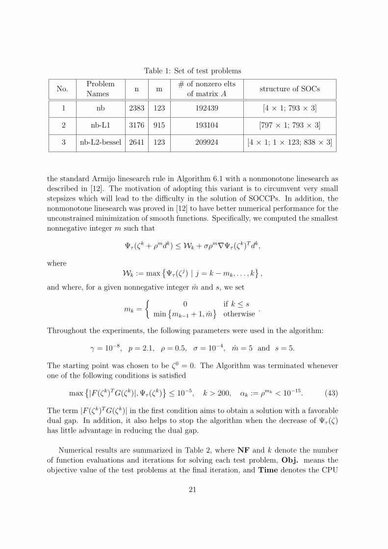
Table 1: Set of test problems

No.Problem

Namesn m

# of nonzero elts

of matrix Astructure of SOCs

1 nb 2383 123 192439 [4 × 1; 793 × 3]

2 nb-L1 3176 915 193104 [797 × 1; 793 × 3]

3 nb-L2-bessel 2641 123 209924 [4 × 1; 1 × 123; 838 × 3]

the standard Armijo linesearch rule in Algorithm 6.1 with a nonmonotone linesearch as

described in [12]. The motivation of adopting this variant is to circumvent very small

stepsizes which will lead to the difficulty in the solution of SOCCPs. In addition, the

nonmonotone linesearch was proved in [12] to have better numerical performance for the

unconstrained minimization of smooth functions. Specifically, we computed the smallest

nonnegative integer m such that

Ψτ (ζk + ρmdk) ≤ Wk + σρm∇Ψτ (ζ

k)T dk,

where

Wk := max{Ψτ (ζ

j) | j = k −mk, . . . , k}

,

and where, for a given nonnegative integer m and s, we set

mk =

{0 if k ≤ s

min{mk−1 + 1, m

}otherwise

.

Throughout the experiments, the following parameters were used in the algorithm:

γ = 10−8, p = 2.1, ρ = 0.5, σ = 10−4, m = 5 and s = 5.

The starting point was chosen to be ζ0 = 0. The Algorithm was terminated whenever

one of the following conditions is satisfied

max{|F (ζk)T G(ζk)|, Ψτ (ζ

k)} ≤ 10−5, k > 200, αk := ρmk < 10−15. (43)

The term |F (ζk)T G(ζk)| in the first condition aims to obtain a solution with a favorable

dual gap. In addition, it also helps to stop the algorithm when the decrease of Ψτ (ζ)

has little advantage in reducing the dual gap.

Numerical results are summarized in Table 2, where NF and k denote the number

of function evaluations and iterations for solving each test problem, Obj. means the

objective value of the test problems at the final iteration, and Time denotes the CPU

21

Table 2: Numerical results of Algorithm 6.1 for linear SOCPs with a different τ

No. τ Obj. NF k Time τ Obj. NF k Time

0.5 –0.0507101 177 59 644.1 1.5 –0.0507184 75 28 303.2

1 2.0 –0.0507130 85 29 313.8 2.5 –0.0507088 66 32 342.2

3.0 –0.0507256 74 29 311.2 3.5 –0.0507091 63 38 406.0

0.5 – – > 200 – 1.5 –13.0122435 144 87 1587.4

2 2.0 –13.0120761 219 112 2047.2 2.5 –13.0121923 227 112 2149.3

3.0 –13.0121999 393 197 3762.1 3.5 – – > 200 –

0.5 –0.1025695 35 18 235.3 1.5 –0.1025728 23 10 128.6

3 2.0 –0.1025766 15 9 113.7 2.5 –0.1025706 17 10 125.6

3.0 –0.1025695 21 14 181.4 3.5 –0.1025695 39 29 364.4

time in second that the iterates satisfy the termination condition.

From Table 2, we see that the semismooth Newton method proposed can solve all

test problems with τ ∈ [1.5, 3] and has better numerical performance with τ ∈ [1.5, 2.5]

for all test problems. When τ tends to 0 or 4, the number of iteration has a remarkable

increase. For problem “nb-L1”, Algorithm 6.1 requires much more iterations. After a

check, the solution of this problem does not satisfy strict complementarity, and now we

are not clear whether this takes charge in much more iterations. We also observe that the

parameter τ close to 4 often gives a better global convergence, whereas the parameter

τ close to 0 leads to a fast local convergence. Figure 1 below displays the convergence

of Ψτ for problem “nb” with τ = 0.1 and τ = 3.9, respectively. The performance of Ψτ

coincides with the case described by [14] for the NCPs, which is very important for the

use of the class of SOC complementarity functions. Based on this feature of φτ , we may

adopt a dynamic choice of τ in the algorithm by following a line similar to [14].

7 Conclusions

In this paper, we continued to investigate the properties of the one-parametric class

of SOC complementarity functions φτ , which includes the FB SOC complementarity

22

0 20 40 60 80 100 120 140 160 180 20010

−6

10−5

10−4

10−3

10−2

10−1

100

101

Iterations

Merit Func values v.s. Iterations

(a) τ = 0.1

0 20 40 60 80 100 120 14010

−8

10−7

10−6

10−5

10−4

10−3

10−2

10−1

100

101

Iterations

Merit Func values v.s. Iterations

(b) τ = 3.9

Figure 1: The convergence of Algorithm 6.1 with different τ for ‘nb’.

23

function and the natural residual SOC complementarity function as a special case. We

showed that φτ is globally Lipschitz continuous and strongly semismooth and charac-

terized its B-subdifferential at any point. Furthermore, for the induced merit function

Ψτ , we provided a weaker condition than [6] to guarantee every stationary point to be

a solution of the SOCCP, and proved that it has bounded level sets for the SOCCP (3)

if the mapping has the uniform Cartesian P -property and satisfies Condition A. Com-

bining with the results of [6], we thus extended most of favorable properties of the class

of complementarity functions for the NCP to the setting of the SOCCP.

A semismooth Newton method is also proposed by the nonsmooth reformulation (10)

involving the class of SOC complementarity functions. The superlinear convergence of

the algorithm is established by requiring the solution to be strict complementarity. The

condition is stronger than the counterpart in the NCPs, and we will consider to weaken

this condition in the future research work.

Acknowledgements The authors would like to thank the two anonymous referees for

their helpful comments which improved the presentation of this paper.

References

[1] F. Alizadeh and D. Goldfarb (2003), Second-order cone programming, Mathe-

matical Programming, vol. 95, pp. 3–51.

[2] E. D. Andersen, C. Roos, and T. Terlaky (2003), On implementing a primal-

dual interior-point method for conic quadratic optimization, Mathematical Program-

ming Ser. B, vol. 95, pp. 249–277.

[3] X. Chen and H. Qi (2006), Cartesian P-proeprty and its applications to the

semidefinite linear complementarity problem, Mathematical Programming, vol. 106,

pp. 177–201.

[4] X.-D. Chen, D. Sun, and J. Sun (2003), Complementarity functions and numer-

ical experiments for second-order cone complementarity problems, Computational

Optimization and Applications, vol. 25, pp. 39–56.

[5] F. H. Clarke, Optimization and Nonsmooth Analysis, John Wiley & Sons, New

York, 1983 (reprinted by SIAM, Philadelphia, PA, 1990).

[6] J.-S. Chen and S.-H. Pan (2007), A one-parametric class of merit functions for

the second-order cone complementarity problem, Submitted to Computational Opti-

mization and Applications.

24

[7] J.-S. Chen and P. Tseng (2005), An unconstrained smooth minimization refor-

mulation of the second-order cone complementarity problem, Mathematical Program-

ming, vol. 104, pp. 293–327.

[8] J. Faraut and A. Koranyi, Analysis on Symmetric Cones, Oxford Mathematical

Monographs, Oxford University Press, New York, 1994.

[9] M. Fukushima, Z.-Q. Luo, and P. Tseng (2002), Smoothing functions for

second-order cone complementarity problems, SIAM Journal on Optimization, vol.

12, pp. 436–460.

[10] A. Fischer (1992), A special Newton-type optimization methods, Optimization,

vol. 24, pp. 269-284.

[11] A. Fischer (1997), Solution of the monotone complementarity problem with locally

Lipschitzian functions, Mathematical Programming, vol. 76, pp. 513-532.

[12] L. Grippo, F. Lampariello and S. Lucidi (1986), A nonmonotone line search

technique for Newton’s method, SIAM Journal on Numerical Analysis, 1986, vol. 23,

pp. 707–716.

[13] S. Hayashi, N. Yamashita, and M. Fukushima (2005), A combined smoothing

and regularization method for monotone second-order cone complementarity prob-

lems, SIAM Journal of Optimization, vol. 15, pp. 593–615.

[14] C. Kanzow and H. Kleinmichel (1998), A new class of semismooth Newton-

type methods for nonlinear complementarity problems, Computational Optimization

and Applications, vol. 11, pp. 227–251.

[15] C. Kanzow and M. Fukushima (2006), Semismooth metods for linear and non-

linear second-order cone programs, Technical Report, Department of Applied Math-

ematics and Physics, Kyoto University.

[16] T. De. Luca, F. Facchinei and C. Kanzow (1996), A semismooth equation

approach to the solution of nonlinear complementarity problems, Mathematical Pro-

gramming, vol. 75, pp. 407–439.

[17] M. S. Lobo, L. Vandenberghe, S. Boyd, and H. Lebret (1998), Application

of second-order cone programming, Linear Algebra and its Applications, vol. 284, pp.

193–228.

[18] R. D. C. Monteiro and T. Tsuchiya (2000) Polynomial convergence of primal-

dual algorithms for the second-order cone programs based on the MZ-family of direc-

tions, Mathematical Programming, vol. 88, pp. 61–83.

25

[19] S.-H. Pan and J.-S. Chen (2006), A damped Gauss-Newton method for the

second-order cone complementarity problem, Accepted by Applied Mathematics and

Optimization.

[20] L. Qi and J. Sun (1993) A nonsmooth version of Newton’s method, Mathematical

Programming, vol. 58, pp. 353–367.

[21] L. Qi (1993) Convergence analysis of some algorithms for solving nonsmooth equa-

tions, Mathematics of Operations Research, vol. 18, pp. 227–244.

[22] D. Sun and L.-Q. Qi, On NCP-functions (1999), Computational Optimization

and Applications, vol. 13, pp. 201-220.

[23] D. Sun and J. Sun (2005), Strong semismoothness of the Fischer-Burmeister

SDC and SOC complmentarity functions, Mathematical Programming, vol. 103, pp.

575–581.

[24] T. Tsuchiya (1999), A convergence analysis of the scaling-invariant primal-dual

path-following algorithms for second-order cone programming, Optimization Meth-

ods and Software, vol. 11, pp. 141–182.

Appendix

Lemma A.1 The function z(x, y, ε) defined by (24) for any ε > 0 is continuously

differentiable everywhere, and there exists a scalar C > 0 such that

‖∇xz(x, y, ε)‖F ≤ C, ‖∇yz(x, y, ε)‖F ≤ C (44)

for all (x, y) ∈ IRl × IRl, where ‖A‖F denotes the Frobenius norm of the matrix A.

Proof. Since (x− y)2 + τ(x ◦ y) + εe ∈ int(Kl) for any (x, y) ∈ IRl × IRl and ε > 0, by

Lemma 2.1 the function z(x, y, ε) is continuously differentiable everywhere and

∇xz(x, y, ε) =

(Lx +

τ − 2

2Ly

)L−1

z , ∇yz(x, y, ε) =

(Ly +

τ − 2

2Lx

)L−1

z . (45)

We next prove the bound in (44) by the two cases: w2 6= 0 and w2 = 0. Let

w = (w1, w2) = w(x, y, ε) := (x− y)2 + τ(x ◦ y) + εe.

Case (1). w2 6= 0. Then, w2 6= 0 since w2 = w2. Let g = (g1, g2) := x + τ−22

y. By (45)

and the formula of L−1z given by (19), we can compute that

∇xz(x, y, ε) =

(bg1 + cgT

2 w2 cg1w2 + agT2 + (b− a)gT

2 w2wT2

bg2 + cg1w2 cg2wT2 + ag1I + (b− a)g1w2w2

),

26

where a, b and c are defined as in Lemma 2.1 with w = w. Notice that

g1 = x1 +τ − 2

2y1, g2 = x2 +

τ − 2

2y2; λ1(w) = λ1(w) + ε, λ2(w) = λ2(w) + ε.

Using the expression of a, b and c and the result of Lemma 2.3 then yields that∣∣∣bg1 + cgT

2 w2

∣∣∣ ≤ 1

2√

λ2(w)

∣∣g1 + gT2 w2

∣∣ +1

2√

λ1(w)

∣∣g1 − gT2 w2

∣∣ ≤ 1,

∥∥∥cg1wT2 + bgT

2 w2wT2

∥∥∥ ≤ 1

2√

λ2(w)

∣∣g1 + gT2 w2

∣∣ +1

2√

λ1(w)

∣∣g1 − gT2 w2

∣∣ ≤ 1,

∥∥agT2 − agT

2 w2wT2

∥∥ ≤ ‖2g2‖√‖x‖2 + ‖y‖2 + (τ − 2)xT y

(1 + ‖w2‖) ≤ 4,

∥∥∥bg2 + cg1w2

∥∥∥ ≤ 1

2√

λ2(w)‖g2 + g1w2‖+

1

2√

λ1(w)‖g2 − g1w2‖ ≤ 1,

∥∥∥cg2wT2 + bg1w2w

T2

∥∥∥F

≤ 1

2√

λ2(w)‖g2 + g1w2‖+

1

2√

λ1(w)‖g2 − g1w2‖ ≤ 1,

∥∥ag1I − ag1w2wT2

∥∥F

≤ 2|g1|√‖x‖2 + ‖y‖2 + (τ − 2)xT y

·∥∥I − w2w

T2

∥∥F≤ 2(l − 1).

The above inequalities imply that the first inequality in (44) holds under this case.

Case (2). w2 = 0. In this case, from Lemma 2.1 it follows that

∇xz(x, y, ε) =1√w1

(Lx +

τ − 2

2Ly

)=

1√w1

Lg.

Since w1 = ‖x+ τ−22

y‖2+ τ(4−τ)4‖y‖2+ε, we have |g1|/

√w1 ≤ 1 and ‖g2‖/

√w1 ≤ 1, which

implies the first inequality in (44). Thus, we complete the proof for the first inequality.

By the symmetry of x and y in z(x, y, ε), the second inequality clearly holds. 2

Proof of Proposition 3.2

Proof. Throughout the proof, let Dφτ denote the set of points where φτ is differentiable.

Recall that this set is characterized by Proposition 3.1 (a). Write

φ′τ,x(x, y) = ∇xφτ (x, y)T and φ′τ,y(x, y) = ∇yφτ (x, y)T .

From Proposition 3.1 (a), it then follows that for any (x, y) ∈ Dφτ ,

φ′τ,x(x, y) = L−1z Lx+ τ−2

2y − I, φ′τ,x(x, y) = L−1

z Ly+ τ−22

x − I. (46)

Moreover, we observe from (19) that, when w2 6= 0, L−1z can be expressed as the sum of

L1(w) =1

2√

λ1(w)

(1 −wT

2

−w2 w2wT2

)

27

and

L2(w) =1

2√

λ2(w)

1 wT2

w2

4√

λ2(w)(I − w2wT2 )√

λ2(w) +√

λ1(w)+ w2w

T2

,

and consequently φ′τ,x and φ′τ,y in (46) can be rewritten as

φ′τ,x(x, y) = (L1(w) + L2(w))Lx+ τ−22

y − I,

φ′τ,x(x, y) = (L1(w) + L2(w))Ly+ τ−22

x − I. (47)

(a) Under the given assumption, φτ is continuously differentiable at (x, y) by Proposition

3.1 (a). Consequently, the B-subdifferential ∂Bφτ (x, y) consists of only one element,

φ′τ (x, y) =[φ′τ,x(x, y) φ′τ,x(x, y)

].

Substituting the formulas in (46) into it, we immediately obtain the conclusion.

(b) Assume that (x, y) 6= (0, 0) satisfies (x−y)2+τ(x◦y) ∈ bd(Kl). Let {(xk, yk)} ⊆ Dφτ

be an arbitrary sequence converging to (x, y). Let wk = (wk1 , w

k2) = w(xk, yk) and zk =

z(xk, yk), where w(x, y) and z(x, y) are defined as in (16). From the given assumption

on (x, y), we have w ∈ bd(Kl) and w1 > 0, which means that λ2(w) > λ1(w) = 0 and

‖w2‖ = w1 > 0. Hence, we assume without loss of generality that wk2 6= 0 for each k.

Using the formulas in (47), it then follows that

φ′τ,x(xk, yk) =

(L1(w

k) + L2(wk)

)Lxk+ τ−2

2yk − I,

φ′τ,y(xk, yk) =

(L1(w

k) + L2(wk)

)Lyk+ τ−2

2xk − I. (48)

Notice that limk→+∞ λ2(wk) = 2w1 > 0 and limk→+∞ λ1(w

k) = λ1(w) = 0, which,

together with limk→+∞ Lxk = Lx, limk→+∞ Lyk = Ly and limk→+∞ wk2 = w2, yields that

limk→+∞

L2(wk)Lxk+ τ−2

2yk = C(w)

(Lx +

τ − 2

2Ly

),

limk→+∞

L2(wk)Lyk+ τ−2

2xk = C(w)

(Ly +

τ − 2

2Lx

), (49)

where C(w) is defined as follows:

C(w) =1

2√

2w1

(1 wT

2

w2 4I − 3w2wT2

)with w2 =

w2

‖w2‖ .

In addition, by a simple computation, we have that

L1(wk)Lxk+ τ−2

2yk =

1

2

(uk

1 (uk2)

T

−uk1w

k2 −wk

2(uk2)

T

),

L1(wk)Lyk+ τ−2

2xk =

1

2

(vk

1 (vk2)

T

−vk1 w

k2 −wk

2(vk2)

T

),

28

where wk2 = wk

2/‖wk2‖ for each k, and

uk1 =

1√λ1(wk)

[(xk

1 +τ − 2

2yk

1

)−

(xk

2 +τ − 2

2yk

2

)T

wk2

],

uk2 =

1√λ1(wk)

[(xk

2 +τ − 2

2yk

2

)−

(xk

1 +τ − 2

2yk

1

)wk

2

],

vk1 =

1√λ1(wk)

[(yk

1 +τ − 2

2xk

1

)−

(yk

2 +τ − 2

2xk

2

)T

wk2

],

vk2 =

1√λ1(wk)

[(yk

2 +τ − 2

2xk

2

)−

(yk

1 +τ − 2

2xk

1

)wk

2

].

By Lemma 2.3, |uk1| ≤ ‖uk

2‖ ≤ 1 and |vk1 | ≤ ‖vk

2‖ ≤ 1. So, taking the limit (possibly on

a subsequence) on L1(wk)Lxk+ τ−2

2yk and L1(w

k)Lyk+ τ−22

xk , we have

L1(wk)Lxk+ τ−2

2yk → 1

2

(u1 uT

2

−u1w2 −w2uT2

)=

1

2

(1

−w2

)uT

L1(wk)Lyk+ τ−2

2xk → 1

2

(v1 vT

2

−v1w2 −w2vT2

)=

1

2

(1

−w2

)vT (50)

for some u = (u1, u2), v = (v1, v2) ∈ IR× IRl−1 with |u1| ≤ ‖u2‖ ≤ 1 and |v1| ≤ ‖v2‖ ≤ 1,

where w2 = w2/‖w2‖. In fact, u and v are some accumulation point of the sequences

{uk} and {vk}, respectively. From (48)–(50), we obtain that

φ′τ,x(xk, yk) → C(w)

(Lx +

τ − 2

2Ly

)+

1

2

(1

−w2

)uT − I,

φ′τ,y(xk, yk) → C(w)

(Ly +

τ − 2

2Lx

)+

1

2

(1

−w2

)vT − I.

This shows that as k → +∞, φ′τ (xk, yk) → [Vx − I Vy − I] with Vx, Vy satisfying (25).

(c) Assume (x, y) = (0, 0). Let {(xk, yk)} ⊆ Dφτ be an arbitrary sequence converging to

(x, y). Let wk = (wk1 , w

k2) and zk be defined as in Case (b). From the given assumptions,

we have w = 0. Therefore, we may assume without any loss of generality that wk2 = 0

for all k or wk2 6= 0 for all k. We proceed the arguments by the two cases.

Case (1): wk2 = 0 for all k. From equation (46) and Lemma 2.1, it follows that

φ′τ,x(xk, yk) =

1√wk

1

(xk

1 + τ−22

yk1

(xk

2 + τ−22

yk2

)T

xk2 + τ−2

2yk

2

(xk

1 + τ−22

yk1

)I

)− I,

φ′τ,y(xk, yk) =

1√wk

1

(yk

1 + τ−22

xk1

(yk

2 + τ−22

xk2

)T

yk2 + τ−2

2xk

2

(yk

1 + τ−22

xk1

)I

)− I.

29

Since

wk1 = ‖xk +

τ − 2

2yk‖2 +

τ(4− τ)

4‖yk‖2 = ‖yk +

τ − 2

2xk‖2 +

τ(4− τ)

4‖xk‖2,

every element in the above φ′τ,x(xk, yk) and φ′τ,y(x

k, yk) are bounded. Thus, taking limit

(possibly on a subsequence) on φ′τ,x(xk, yk) and φ′τ,y(x

k, yk), respectively, gives

∇xφτ (xk, yk) →

(u1 uT

2

u2 u1I

)− I, ∇yφτ (x

k, yk) →(

v1 vT2

v2 v1I

)− I

for some u = (u1, u2), v = (v1, v2) ∈ IR × IRl−1 satisfying ‖u‖ ≤ 1, ‖v‖ ≤ 1 and

u1v2+v1u2 = 0. This shows that φ′τ (xk, yk) → [Vx−I Vy−I] with Vx ∈ {Lu}, Vy ∈ {Lv}.

Case (2): wk2 6= 0 for all k. Now φ′τ,x(x

k, yk) and φ′τ,y(xk, yk) are given as in (48). Using

the same arguments as part (b) and noting that {wk2} is bounded, we have

L1(wk)Lxk+ τ−2

2yk → 1

2

(1

−w2

)uT , L1(w

k)Lyk+ τ−22

xk → 1

2

(1

−w2

)vT (51)

for some vectors u = (u1, u2), v = (v1, v2) ∈ IR × IRl−1 satisfying |u1| ≤ ‖u2‖ ≤ 1 and

|v1| ≤ ‖v2‖ ≤ 1, and w2 ∈ IRl−1 satisfying ‖w2‖ = 1. We next compute the limit of

L2(wk)Lxk+ τ−2

2yk and L2(w

k)Lyk+ τ−22

xk . By the definition of L2(w),

L2(wk)Lxk+ τ−2

2yk =

1

2

(ξk1 (ξk

2 )T

ξk1 wk

2 + 4(I − wk2(w

k2)

T )sk2 wk

2(ξk2 )T + 4(I − wk

2(wk2)

T )sk1

),

L2(wk)Lyk+ τ−2

2xk =

1

2

(ηk

1 (ηk2)

T

ηk1 w

k2 + 4(I − wk

2(wk2)

T )ωk2 wk

2(ηk2)

T + 4(I − wk2(w

k2)

T )ωk1

)

where

ξk1 =

1√λ2(wk)

[(xk

1 +τ − 2

2yk

1

)+

(xk

2 +τ − 2

2yk

2

)T

wk2

],

ξk2 =

1√λ2(wk)

[(xk

2 +τ − 2

2yk

2

)+

(xk

1 +τ − 2

2yk

1

)wk

2

],

ηk1 =

1√λ2(wk)

[(yk

1 +τ − 2

2xk

1

)+

(yk

2 +τ − 2

2xk

2

)T

wk2

], (52)

ηk2 =

1√λ2(wk)

[(yk

2 +τ − 2

2xk

2

)+

(yk

1 +τ − 2

2xk

1

)wk

2

],

and

sk1 =

(xk

1 + τ−22

yk1

)√

λ2(wk) +√

λ1(wk), sk

2 =

(xk

2 + τ−22

yk2

)√

λ2(wk) +√

λ1(wk);

ωk1 =

(yk

1 + τ−22

xk1

)√

λ2(wk) +√

λ1(wk), ωk

2 =

(yk

2 + τ−22

xk2

)√

λ2(wk) +√

λ1(wk). (53)

30

By Lemma 2.3, |ξk1 | ≤ ‖ξk

2‖ ≤ 1 and |ηk1 | ≤ ‖ηk

2‖ ≤ 1. In addition,

‖sk‖2 + ‖ωk‖2 =‖xk + τ−2

2yk‖2 + ‖yk + τ−2

2xk‖2

2[‖xk‖2 + ‖yk‖2 + (τ − 2)(xk)T yk] + 2√

λ2(wk)√

λ1(wk)≤ 1.

Taking the limit on L2(wk)Lxk+ τ−2

2yk and L2(w

k)Lyk+ τ−22

xk , we have

L2(wk)Lxk+ τ−2

2yk → 1

2

(ξ1 ξ2

ξ1w2 + 4(I − w2wT2 )s2 w2ξ

T2 + 4(I − w2w

T2 )s1

)

=1

2

(1

w2

)ξT + 2

(0 0

(I − w2wT2 )s2 (I − w2w

T2 )s1

)(54)

L2(wk)Lyk+ τ−2

2xk → 1

2

(η1 η2

η1wT2 + 4(I − w2w

T2 )ω2 w2η

T2 + 4(I − w2w

T2 )ω1

)

=1

2

(1

w2

)ηT + 2

(0 0

(I − w2wT2 )ω2 (I − w2w

T2 )ω1

)(55)

for some vectors ξ = (ξ1, ξ2), η = (η1, η2) ∈ IR × IRl−1 satisfying |ξ1| ≤ ‖ξ2‖ ≤ 1 and

|η1| ≤ ‖η2‖ ≤ 1, and s = (s1, s2), ω = (ω1, ω2) ∈ IR × IRl−1 satisfying ‖s‖2 + ‖ω‖2 ≤ 1.

From equations (51), (54) and (55), it follows that as k → +∞,

φ′τ,x(xk, yk) → 1

2

(1

w2

)ξT +

1

2

(1

−w2

)uT + 2

(0 0

(I − w2wT2 )s2 (I − w2w

T2 )s1

)− I,

φ′τ,x(xk, yk) → 1

2

(1

w2

)ηT +

1

2

(1

−w2

)vT + 2

(0 0

(I − w2wT2 )ω2 (I − w2w

T2 )ω1

)− I.

This shows that as k → +∞, φ′τ (xk, yk) → [Vx − I Vy − I] with Vx and Vy satisfying

(26). Combining with Case (1), the desired result then follows. 2

31