A semilinear wave equation associated with a linear differential equation with Cauchy data

Pergamon Nonlinear Analysis, Theory, Methods & Applications, Vol. 24, No. 8, pp. 1261-1279, 1995

Copyright © 1995 Elsevier Science Ltd Printed in Great Britain. All rights reserved

0362-546X/95 $9.50 + .00

0362-546X(94)00196-0

A S E M I L I N E A R W A V E E Q U A T I O N A S S O C I A T E D W I T H A

L I N E A R D I F F E R E N T I A L E Q U A T I O N W I T H C A U C H Y D A T A

NGUYEN THANH LONGt and ALAIN PHAM NGOC DINH~:

tDepar tment of Mathematics, Polytechnic University of Ho Chi Minh City, 268 Ly Thuong Kiet, district 10, Ho Chi Minh City, Viet-Nam; and

~tCNRS-URA 1803; D6partment of Math6matiques, Universit6 d'Orl4ans BP 6759; 45067 - Orl6ans, Cedex, France

(Received 10 March 1993; received in revised form 16 January 1994; received for publication 17 August 1994)

Key words and phrases: Global existence, nonlinear Volterra integral equation, uniqueness of the solution, stability of the solutions, numerical results.

1. I N T R O D U C T I O N

In this paper we consider the following problem. Find a pair (u, P) of functions satisfying

U t t - - U x x - i - f ( u , u t ) = O , O < x < l , O < t < T , (1.1)

ux(O, t) = e ( t ) (1.2)

u(1, t) = 0 (1.3)

u(x,O) = u0(x); ut(x,O) = Ul(X), (1.4)

where u0, Ul, f are given functions satisfying conditions to be specified later, and the unknown function u(x, t) and the unknown boundary value P(t) satisfy the following Cauchy problem for ordinary differential equations

P"(t)+to2p(t)=hutt(O,t) , 0 < t < T (1.5)

P(0) =P0, P'(0) =el, (1.6)

where to > 0, h _> 0, P0, Pt are given constants. In [1], An and Trieu studied a special case of the problem (1.1)-(1.6) with u 0 = u I = P0 = 0

and with f(u, u,) linear, i.e. f(u, u,) = Ku + Au, where K, A are given constants. In the latter case this problem is a mathematical model describing the shock of a rigid body and a linear viscoelastic bar resting on a rigid base. Our problem is thus a nonlinear analogue of the problem considered in [1].

In the case where f (u ,u t) = lu,I ~- lu t the problem (1.1)-(1.6)governs the shock between a solid body and a linear viscoelastic bar with nonlinear elastic constraints at the side, constraints associated with a viscous frictional resistance.

From (1.5) and (1.6) we represent P(t) in terms of Po, P1, to, h, utt(O,t) and then by integrating by parts, we obtain

fo ' P(t) -- g(t) +hu(O,t) - k(t - s )u (O,s )ds , (1.7)

1261

1262 NNGUYEN THANH LONG and A. PHAM NGOC DINH

where

g ( t ) = (eo + huo (0)) cos tot + I ( P 1 - h u l ( O ) ) sin tot (1.8) to

k ( t ) = h to sin to t. (1.9)

By eliminating an unknown function P(t ) , we replace the boundary condition (1.2) by

~0 t ux(O, t ) - -g( t ) + h u ( O , t ) - k ( t - s ) u ( O , s ) d s . (1.10)

Then, we reduce problem (1.1)-(1.6) to (1.1)-(1.4), (1.7)-(1.9) or (1.1), (1.3), (1.4), (1.8)-(1.10). In [2], Ang and Dinh established a uniqueness and global existence for the problem (i.b.v)

(1.1), (1.3), (1.4), (1.10) with

h = O, k ( t ) - 0 (1.11)

f(u,ut)=lu,l~-lu,, 0 < a < l . (1.12)

In [3] we established results about global and local existence of solutions for problem (i.b.v) (1.1), (1.3), (1.4), (1.10) with

• k ( t ) = O, h > 0 ( g ( t ) given) (1.13)

• function f ( u , u t) H61der continuous with respect to each variable and nondecreasing with respect to u r This case contains the case (1.12) as a special case.

The aim of this paper is to prove three theorems. In theorem 1, global existence and uniqueness of a solution of the problem (1.1), (1.3), (1.4), (1.10) are proved. In theorem 2, we prove that the solution (u, P) of this problem is stable with respect to the parameter h > 0 and the functions g( t ) and k( t ) . In theorem 3, we prove that the solution of problems (1.1)-(1.6) is also stable with respect to the real parameters h > 0, to > 0, P0, Pa.

Finally, we present some numerical results.

2. U N I Q U E N E S S AND E X I S T E N C E T H E O R E M S

First, we set some notations

II = (0,1), Q r = I I × ( O , T ) , T > 0

L q = L q ( ~ ) , H 1 = Hl ( f~) ,

where H ~ is the usual Sobolev space on IL Let ( . , . ) be either the scalar product in L 2 or the dual pairing of a continuous linear

functional and an element of a function space. The notation ll'lf stands for the norm in L 2 and we denote by If'llx the norm in the Banach

space X. We call X ' the dual space of X. We denote by LP(0, T; X) , 1 < p _< oo for the Banach space of the real functions f:(0, T) ~ X

measurable, such that

(j0 I l f l lL ,¢0 , r ; x ) -- I I f ( t ) l l x e dt < ~, for 1 < p < oo

Semilinear wave equation 1263

or

We put

IlfllL®(0,T;X) = ess supllf(t)llx, 0<t<T

forp = oo.

V = {v e H l / v ( 1 ) = 0}

a(u,v) = ( Ou ,~v } f~ Ou Ov c~ x ' c~ x = c~----~ ~---~ d x .

V is a closed subspace of H 1 and on V, IIvlIH, and a¢-~, v) are two equivalent norms. We put

Ilvll, = ~ v ) .

We then have the following lemma.

LEMMA 1. The imbedding Vc_, C°(K) is compact and

Ilvllc0(~) _< Ilvllo, Vv ~ V.

The proof is straightforward and we omit the details. We make the following assumptions: (A 1) u o ~ H 1, U l E L 2 ; (A 2) h > 0 ; (A 3) g ~HI(O,T) , V T > 0 and g(0) exists; (m 4) k ~ H I ( O , T ) , V T > 0 and k(0)=0. The function f : R 2 ~ R satisfies f(0, 0)= 0 and the following conditions: (F 1) ( f ( u , v ) - f ( u f ) ) ) ' ( v - ~ ) > O , Vu, v, ~ e R ;

there are two constants a, /3~(0,1) and two functions Bl, B 2 : R + ~ R + satisfying:

(F 2) B 1 is nondecreasing; (F 3) B2(IvI)eL2(QT), Vv EL2(QT), VT> O; (F4) If(u, v)-f(u, ~)1 ~Bl(lul)lv-DI ~, (Fs) If(u,v)-f(a,v)l~B2(Ivl)lu-~l r3, We also use the notations

Vu, v,b e R ; Vu, fi, v ~ R.

3u O2u t ~ - - U t t

l ~ = l.,I t c ~ t ' = u t t egg 2 "

Then, we have the following theorem.

(2.1)

continuous and

THEOREM 1. Let (AI)-(A 4) and (F1)-(F 5) hold. Then, for every T > 0, there exists a weak solution (u, P) of problem (1.1)-(1.4) and (1.7),

such that

u ~ L = ( O , T ; V ) , ut~L°~(O,T;L2), u t (O , t )~L2(O,T) (2.2)

P ~ Hi(0, T). (2.3)

Furthermore, if /3 = 1 in (Fs), the solution is unique.


Remark. This result is stronger than in [3]. Indeed, corresponding to the same problems (1.1)-(1.4) and (1.7) with k(t) = O, the following assumptions which were made in [3] are not needed here

2

0 < a < l , BI( lu l )~LI -~(Qr) , Vu~L~(O,T:V) , V T > 0 . (2.4)

B 2 is nondecreasing. (2.5)

Proof The proof consists of several steps.

Step 1. The Galerkin approximation. Consider a special orthonormal basis on V

= ~f 2 "cos(Ajx), Aj = (2j - 1) 2 , j = 1,2,. 2 "" ~ ( x ) 1 +Aj

formed by the eigenfunctions of the Laplacian --(o~2//tgX2).

Put

Um(t) = ~ Cmj(t)Wj, (2.6) j=l

where cmj(t) satisfy the following system of nonlinear differential equations

(U"m(t),Wj) + a(Um(t), Wj) + Pro(t). Wi(O) + ( f(um(t) , U'm(t)) , W i) = 0

Vj, 1 < j < m (2.7)

Pro(t) = g ( t ) +h.um(O,t) - k( t -s )um(O,s)ds (2.8)

Urn(O) = Uom = ~ amj ~ ~ U o strongly in H 1 ]=1

(2.9) U'm(O) = Ulm = ~ Bmj~ ~ Ul strongly in L 2.

j=l

For fixed T > 0, from the assumptions of the theorem, system (2.7)-(2.9) has solution (u,,(t), Pro(t)) on an interval [0, Tml- The following estimates allow one to take Tm = T for all m .

Step 2. A priori estimates. Substituting (2.8) into (2.7), then multiplying the jth equation of (2.7) by C'mj(t) and summing up with respect to j, we have

1 7S re(t) 4- (f(Um(t),U'm(t)) --f(Um(t),O) , U'm(t)) = --g(t)u'm(O,t)

-(f(Um(t),O),U'm(t)) + k(t-S)Um(O,s)ds.u'm(O,t) , (2.10)


where

S,,(t) = IlU'm(t)[I 2 + Ilum(t)ll2o + hu2(O, t). (2.11)

Using the assumption (F 1) about the monotony with respect to the second variable and the assumption (m3) , then integrating by parts with respect to the time variable, we have

f0 t Sin(t) < Sm(O) + 2g(0)U0m(0) -- 2g(t)um(O, t) "~ 2 g'(S)Um(O, S)ds

fo' -- 2 (f(Um(S),O) , U'm(S) ) as (2.12)

fOt fO "r + 2 u'm(0, I") d~" 2k(r-S)Um(O,s)ds.

Using (2.9), (2.11) and lemma 1 we get

Ci S,,(O) + 2lg(O)Uom(O)l <_ -if-, Vm, (2.13)

where C 1 is a constant independent from m. Again using lemma 1 and the inequality

a 2 2ab < -~- + 3b 2, Va, b ~ R (2.14)

we obtain

-2g(t)Um(O, t) + 2 g'(S)Um(O, < 3g2(t) + ~Sm(t)

+ 3 Ig'(s)lads + "~ Sin(s) ds. (2.15)

Assumption (F s) implies that

If(u,,(t),O)l < n2(O)llu,,(t)ll~. (2.16)

Using the Cauchy-Schwarz inequality, we obtain in view of (2.11) and (2.16)

(I+/3)

fo fo 12 (f(u,~(s),O),um(s))dsl_2B2(O) SIn(S) ; ds. (2.17)

Note that the last integral in (2.12) gives after integrating by parts

11 = 2um(0,t) k(t -s)um(O,s)ds

- 2 um(0, r ) d r k'(r-S)Um(O,s)ds. (2.18)

1266

Hence

NNGUYEN THANH LONG and A. PHAM NGOC DINH

fot for IIl1~ 2 ~ Ik(t-s)lv~m(s)ds+2 V/~(z) d~ "

× Ik'(w-s)lf~m(S) ds =J1 +J2. (2.19)

The first term in the RHS of (2.19) is estimated by means of the inequality (2.14)

fo f0 J1 <- ½Sin(t) + 3 k2(0) dO Sm(s) ds. (2.20)

Similarly, the second term in the RHS of (2.19) is estimated by means of the Cauchy-Schwartz inequality

1 f0t f0 t f0 t J2 <: -~ Sm('r) d ' r - 3t Ik'(0)l 2 dO- Sm(S)ds. (2.21)

From (2.19) to (2.21) we obtain

lfo' II~ <_ 1Sin(t) + -~ S,.(~') dr

+ 3( fotk2(O)dO+t fotlk'(o)lZ do) fotSm(S)ds. (2.22)

It follows from (2.12), (2.13), (2.15), (2.17), (2.18) and (2.22) that

-- fot fotgm('r )(l +B )/2 dT, Sm(t) <gl( t ) +gz(t) SIn(Z) d~'+ 6B2(0) (2.23)

where

( j0 t ) gl(t) = C 1 + 9 g2(t) + Ig'(s)12ds (2.24)

Since H1(0, T) ~ C°[0, T], from the assumptions (A3), (A 4) we deduce that

Igi(t)l _< M~r i), a.e. t ~ [0, T], (i = 1,2), (2.26)

where M~r i) is a constant depending only on T. It follows, therefore, from (2.23) and (2.26) that

f'e Sin(t) < A'~(1) + - "'-r (Sm(z)) dr, O<t<Tm<r,_ _ (2.27)


where

I ( ( S ) = M(T2)'S + 6B2(0)s 0 + ~)/2 (2.28)

Now/((s) is nondecreasing for s > 0, hence we have

Sm(t)<S(t), Vt ~ [0, T], for every T > 0 (2.29)

since S(t) is the maximal solution of the nonlinear Volterra integral equation with nondecreasing kernal [4] on an interval [0, T] given by

S(t) = M(r ~) + I((S(r)) dr. (2.30)

Now, we need an estimate on the integral JR lU'm(O, s)l 2 ds. Put

Kin(t) = ~ sinAjt

j= 1 Aj (2.31)

[ Tm ( t ) = E Wj(0) Olmj cos Ajt + fl,.j j=

(2.32) m fotSin[Aj(t_r)](Aj ~WJ ) - ¢ j2 I(Um(r),u'm(r)),

Then urn(0, t) can be rewritten as [2]

f0 ' um(O,t) = Tin(t) - g m ( t - r ) P m ( r ) d r . (2 .33)

We shall require the following lemmas.

LEMMA 2. There exist a constant C 2 > 0 and a positive continuous function D(t) independent of m such that

f0' f0' [y'm(S)12ds<C2+D(t) ]lf(Um(S), U'm(S))[12ds

Vt ~ [0, T] for any T> 0. (2.34)

The proof of lemma 2 can be found in [2].

LEMMA 3. There exist two positive constants M~r 3) and M~r 4) depending only on T such that

f0 f0' ~)Pm(r)d'2 f0 'd f''" m(°'r)'2 t d s K ' m ( s - -< ""Ta/tO) + M(T 4) S ' d r .~o

Vt~ [0, T] for any T > 0 . (2.35)

1268

Proof.

then

NNGUYEN THANH LONG and A. PHAM NGOC DINH

Integrating by parts, we have

Y0 Y0 K'm( s - r)pm(r)dr=Km(S)Pm(O ) + Km(S - r)p'm(z)d~ (2.36)

fotds i foSK'm(S - "r ) Pm( ~" ) d'r 2

fot f o t f o s fo s < 2/ '2(0) K~(s)ds + 2 ds K2m(O)dO IP'm(Z)[ 2 d~'. (2.37)

Noticing from (2.8) we have

Pro(O) = g(O) + huom(O)

fo • P'm(r) = g ' ( r ) +hu'm(O,r) - K'm(r-r)um(O,r)dr. (2.38)

Using the inequality (a + b + c) 2 < 3(a 2 + b 2 + c2), Va, b, c ~ R we have

[e'm(~')[2 d~" < 3 [g'(z)lZdz+3h e [U'm(O,z)12dz+3s [k'(O)12dO

X u~(O, r) dr. (2.39)

It follows from (2.37), (2.38) and (2.39) that

fo tdS fo g'm(S-'l')Pm(T) <6 g2(O)dO (g(O)--J-huom(O))2q-t [g ' ( ' r )12d' /"

f o t f o s t2fot fot ] +h e ds [U'm(O,r)12dz + -~ [k'(O)12 dO u~(O,r)dr . (2.40)

Noticing that for every T > 0, Kin(t)-o K(t) strongly in L2(0, T) as m ~ oo, and using the assumptions (A1)-(A 4) and the results (2.13) and (2.29) we obtain (2.35). The lemma 3 is proved completely. •

LEMMA 4. There exist two positive constants M~ 5) and Mtr 6) depending only on T such that

0 t [U 'm(0, S)[ 2 ds < Mtr 5),

f0 ' IP"(s)12 ds < A,¢~6) _ ~,1T ,

Vt ~ [0, T], for any T > 0 (2.41)

¥ t ~ [0, T], for any T > 0 . (2.42)

Proof. From (2.33) we have

U'm(O, t) = y ' m ( t ) - 2 K 'm( t - r ) P m ( r ) dr. (2.43)

From (2.43), using lemmas 2 and 3, we obtain

[u'm(0, s)l 2 ds _< 2C 2 + 2D( t ) f (Um('r) , U ' m ( ~ - ) ) l l 2 d ~ -

yotfo s + 8MCr a~+ 8Mp~ ds lu'm(0, r) l 2 dr . (2.44)

On the other hand, from the assumptions (Fz)-(F 5) we have

[]f(Um(t), U'm(t))l[ 2 <_ 2BE(llu'm(t)llo)[lu',~(t)[[2% + 2BE(O)llum(t)[lEv t3 (2.45)

since 0 < a < 1 we have [ l ' [ [L 2a _~< II-[IL 2 So, using (2.29) and (2.45) we have

[If(urn(t), U'm(t))[[ 2 < 2 B 2 ( x / ~ ) S ° ( t ) + 2B~(O)St~(t) . (2.46)

Finally, from (2.44) and (2.46) we obtain

/o /o'/o lu'm(0, s)l 2 ds < 8M(T 7) + 8M(T 4) ds [u',,(0, ~')l 2 d~'. (2.47)

Inequality (2.41) follows from Gronwall's lemma. Lemma 4 is proved completely. •

Step 3. The limiting process. From (2.8), (2.11) (2.29), (2.41), (2.42) and (2.46), we deduce that, there exists a subsequence of sequence {urn, Pro}, still denoted by {Um, P,,}, such that


Since (2.42) is consequence of (2.29), (2.39) and (2.41), we only have to prove (2.41).

m L~(0, T; V) weak* (2.48)

m L=(0, T; L 2 ) weak* (2.49)

in L°(0, T) weak* (2.50)

m L2(0, T) weak (2.51)

m E=(0, T; L 2) weak* (2.52)

in Hi(0 , T) weak. (2.53)

By the compactness lemma of Lions ([5], p. 57), we can deduce from (2.29), (2.41), (2.48) and (2.49) that there exists a subsequence still denoted by {u m} such that

urn(0, t) ~ u(0, t) strongly in C°([0, T]) (2.54)

u m --* u strongly in LE(Qr) and a.e. (x, t) in Qr. (2.55)

U m - ' ) U

Utm ---> i~ r

u,.(O, t) --, u(O, t)

U'm(O,t) --, u ' (O,t )

/(Urn, U'm) -~ X


From (2.8) and (2.54) we have

fo' Pm(t) ~ g ( t ) +hu(O,t) - k( t - s ) u ( O , s ) d s =-P(t) strongly in c°([o, rl). (2.56)

From (2.53) and (2.56) we have

P=-I 5 a.e. in [0, T]. (2.57/

Passing to the limit in (2.7) by (2.48), (2.49), (2.52) and (2.56) we have

d d - - i ( u ' , v ) + a ( u ( t ) , v ) + P ( t ) v ( O ) + ( X , v ) = O , V v ~ V . (2.58)

Since u, u m ~ C°(O, T;L2), we have Urn(O) ~ u(O) strongly in L 2. Thus

u(0) = u 0. (2.59)

On the other hand, (U 'm( t ) ,W j ) and (u'(t),Wj) belong to C°(O,T). Therefore, (u 'm(0) - u'(0), Wj) ~ 0, as m ~ oo. Hence

u'(0) = u I . (2.60)

Then, in order to prove the existence of the solution of the problems (1.1)-(1.4) and (1.7), we only have to prove that: X =f(u, u').

We shall now require the following lemma.

LEMMA 5. Let u be the solution of the following problems

u" - Uxx + X = 0 (2.61)

ux(0, t) = P ( t ) ; u(1, t) = 0 (2.62)

u(x, 0) = u0(x); u'(x, 0) = ul(x) (2.63)

u ~L~(O,T;V) and u' ~L~(O,T;L2). (2.64)

Then we have

lllu'(t)[[2 + 1 2 f0t f0 t ~llu(/)llv + P(s)u'(O, s) ds + (X(S) , u '(s)) ds

1 2 >- ½11Ulll 2 + ~llu01lv a.e. t ~ [0, T]. (2.65)

Furthermore, if u 0 = u 1 = 0 there is equality in (2.65). The proof of lemma 5 can be found in [2]. We now return to the proof of the existence of a solution of the problem (1.1-(1.4) and

(1.7). It follows from (2.7)-(2.9) that

f0 t t 1 (f(Um(S), u re(S)), U'm(S))ds = ½11Ulmll 2 + ~llu0mll2o _ ½[[U,m(t)[[2 _ _~[[Um(t)[[ 2

fo ' l , m ( - s)u re(O, s) ds. (2.66)


By lemma 5 we have

f0 t r 1 2 l imsup (f(U,n(S),U ,.(S)), u' , .(s))ds _< ½llulll 2 + ~lluoliv - ½ l l u ' ( t ) l [ 2 - ~ [ l u ( t ) l l v l 2 m ~

(2.67)

Y0 - P(s)u'(O, s) ds <_ (X( s ) , u '(s)) ds, a.e. t ~ (0, r ) .

By using the same arguments as in [3] we can show that

x = f ( u , u ' ) a.e. in Qr-

Step 4. Uniqueness of the solution. Assume now that /3 = 1 in (Fs). Let (ul, P1), (u 2, P2) be two solutions of the problem (1.1)-(1.4) and (1.7). Then u = u 1 - u 2 and P = P1 - P2 satisfy the following problem

u" - U x x + X = O , O < x < l , O < t < T

u~(O,t) = P ( t ) ; u (1 , t ) = 0

u(x,O) = u'(x,O) = 0

X =f(u~, u'l) - f ( u 2 , u'2)

P(t) = Pl(t) - Pz(t) = hu(O, t) - k( t - s)u(O, s) ds (2.68)

u i ~ L ~ ( O , r ; v ) , u ' i~L~(O,r;L2) , u ' i ( O , t ) ~ L z ( o , r )

P i~HI(O,T) , i = 1,2.

By using lemma 5 with u o = u 1 = g ( t ) = 0, we obtain

f0 ½1[u'(t)ll 2 + gllu(t)llo + P(s)u'(O, s) ds + (X(S) , u'(s)) ds = 0. (2.69)

Put

Substituting P(t), X respect to the second variable, we have

o-(t) < 2 Ilf(ul(s),u'2(s)) - f(uz(s),u'2(s))l l ' l lu'(s)l lds

fo Yo + 2 u'(O,s)ds k ( s - r ) u ( O , r ) d r .

From assumption (F 5) it follows that

I I f ( u l ( s ) , u ' 2 ( s ) ) - - f ( u 2 ( s ) , U'z(s))ll <_ IIn2(lu'2(s)l)ll" Ilu(s)llv.

~r(t) = Ilu'(t)ll 2 + Ilu(t)llZv + hu2(O, t). (2.70)

into (2.69) and noticing that the function f is nondecreasing with

(2.71)

(2.72)


Using integration by parts in the last integral of (2.71) we get

J= 2u(O,t) k ( t - r )u(O,r )dr - 2 u(O,s)ds k'(s-r)u(O,r)dr. (2.73) " 0

It follows from (2.70) and (2.73) that

S0 f0 IJ] < lo ' ( t ) + 2 k2(O)dO, o'( r ) dr

(So)' s0 + 2f[ ]k'(O)]2dO • ~r(r) dr. (2.74)

Put

T ( f0 T \ 1/2 m(s)=2llBz(lU'z(s)l)[l+4 fo kz(O)dO+4vC-T 'k'(O)12dO) "

Hence, from (2.71) to (2.75), we deduce that

[ ~(t) < m(s)o(s)ds,

i.e. o" - 0 by Gronwall's lemma. The theorem 1 is proved completely. •

(2.75)

3. STABILITY OF THESOLUTIONS

In this section, we assume that /3 = 1. By theorem 1 the problems (1.1)-(1.4) and (1.7) admits a unique solution (u, P) depending on the data h, g, k

u =u(h,g,k), P=P(h,g,k) , (3.1)

where h, g, k satisfy the assumptions (m2)-(m 4) and u0, Ul, f are fixed functions satisfying (A1), (FI)-(Fs).

Then we have the following theorem.

THEOREM 2. Let /3 = 1 and let (A1), (F1)-(Fs) hold. Then, for every T > 0, solutions of the problems (1.1)-(1.4) and (1.7) are stable with respect

to the data h, g, k, i.e.

if (h, g, k), (hi, gj, k ) satisfy the assumptions ( A 2 ) - ( A 4) such that

(hj,gj ,k)~(h,g,k)inR*+xHl(O,T)xHi(O,T)stronglyas j ~ (3.2)

then

(u j, u~, uj(O, t), ~ ) ~ (u, u ' , u(O, t), P )

inL=(O,T;V) XL=°(O,T;Lz)XC°[O,T]XC°[O,T] strongly, as j ~ ~, (3.3)


where

R*+ = (h / h > 0}

u i = u ( h i , g j , k j ) , P j = P ( h j , g i , k j ) .

Proof. First, we note that, if the data (h, g, k) satisfy the assumptions (A2)- (A 4) and

0 < h < H o, IlgllH'¢0,r~ < Go, [Ik[lHko,r) < Ko (3.4)

then, the a priori estimates of the sequences {urn} and {Pro} in the proof of the theorem 1

satisfy

IlU'm(t)ll2+[lUm(t)ll2v<Mr, V t ~ [ O , T ] , V T > O (3.5)

f0 t lu'm(0, s)l 2 ds < M r, Vt ~ [0, T], V T > 0 (3.6)

o t l p ' m ( s ) 1 2 d s < M r , V t ~ [ O , T ] , V T > O , (3.7)

where M r is a constant depending only on T, u 0, u 1, H 0, G 0, K 0 (independent of h, g, k). Hence, the limit (u, P) in suitable function spaces of the sequence (u m, Pro) is defined by

(2.7)-(2.9) and is a solution of the problem (1.1)-(1.4) and (1.7) satisfying the a priori estimates (3.5)-(3.7).

Now, by (3.2) we can assume that, there exist constants H 0 > 0, G O > 0, K 0 > 0 such that the data (hi, gj, kj) satisfy (3.4) with (h, g, k) = (hi, gi' ki)" Then, by the above remark, we have that the solutions (u j, ~ ) of problem (1.1)-(1.4) and (1.7) corresponding to (h, g, k) = (hi, gj, k j) satisfy

Ilu~(t)ll 2 + Iluj(t)ll2o < M r , Vt ~ [0, T], VT > 0 (3.8)

f0 t lug(0, S)I 2 ds < M r , Vt ~ [0, T], V T > 0 (3.9)

£ t IP} (s)12 ds < M r, Vt ~ [0, T], V T > 0. (3.10)

Put

f~j = h i - h, ~,~ = gj - g, fcj = kj - k.

Then, vj = uj - u and Qj = Pi - P satisfy the following problem

n v j - V j x x + X j = O , O < x < l , O < t < T

Vjx(O, t) = Qj( t )

(3.11)

(3.12)

vj(1, t) = vj(x,O) = v~(x,O) = O,


where

xj =f(uj,u;) - f ( u , u ' )

Oj(t) =~j ( t ) +hvj(O,t) - k ( t - s ) v j (O , s )ds (3.13)

~j(t) =~ j ( t ) +hj.uj(O,t) - ~:j(t - s )u j (O , s )ds . (3.14)

By lemma 5 with u o = u 1 = 0, X -- Xi, P = Qj we have

Ilv;(t)ll2 +vj(t)ll~ + 2 Qj(s)v;(O,s)ds + 2 ( Xj,v~)ds=O. (3.15)

Let

~ ( t ) = IIv;(t)ll 2 + Ilvy(t)ll2o + Ivy(0, t)l 2 (3.16)

then, we can prove the following inequality in a similar manner.

1 2 for fot ½ ~ ( t ) < ( E l + E 2 ) ~ ( t ) + - ~ l ~ , j ( t ) l + I~(s)12 ds + o~(s) ds

[Jo Jo ] t t t + ~ k2(s) ds + 2 ~ Ik'(s)lZds × ~ ( s ) ds (3.17)

fo' + IIB2(lu'(s)l)ll%.(s)ds for all /1 >0 , E2 > 0 and Vt ~ [0, T]

choosing E1 +E2 < 1/2. Noting that Hi(0, T) c__, C°[0, T], we have from (3.17) that

(1) ^ 2 f t ~ ( t ) < C r Ilgjlltt,~O,T) + m ( s ) ~ ( s ) ds, (3.18)

" 0

where C~ 1) is a constant depending only on T and

1 [ 1 2 ] re(s) = 21 ( E1 + E2 ) 1 -q- E--~llkllL2~o r ) + 2fTIIk'llL2(0,r) + IIBz(lu'(s)l)ll • (3.19)

By Gronwall's lemma, we obtain from (3.18) that (2) ^ 2 ~ ( t ) < C r ]lgjllnl~o.z), V ~ [0, T]. (3.20)

On the other hand, from (3.13) we obtain

IQi(t)l -< I~(/)1 + h. ~/-~j(t) + IIklIL2~0,T) (S) ds. (3.21)

We again use the embedding Ha(0, T) ~ C°[0, T]. Then, it follows from (3.20) and (3.21) that

IIQ~llco~0, T)-< C~3)ll~jllw~o,T). (3.22) As a final step, we prove

!im II~jll~0,7-) = 0. (3.23)


Indeed, from (3.14) and combined with (3.9), we deduce the following inequality

/,-,(4) [ ~2 - 2 ] II~tllHl(0,r~ --< "~T ["t + Ilgtllm~0.r~ + Ilktl121(0,r~_. (3.24)

The proof of theorem 2 is complete. •

The following theorem is the consequence of theorem 2.

THEOREM 3. Let /3 = 1 and let (A1), (F1)-(F s) hold. Then, for every T > 0, the solutions of the problems (1.1)-(1.6) are stable with respect to

the real parameters h > 0, to > 0, P0, P1, i.e. if (h, to, Po, P1), (ht, tot' Pot, Pit) ~ R2 x R* x R x R such that

(hi, %, Poj,Plj) --, (h, to, Po, PJ) in e 4 (3.25)

then

(uj, u~, uj(O, t), Pj) --. (u ,u ' , u(O, t), P) (3.26)

in L~(0, T; V) × L~(0, T; L 2) × C°[0, T] × C°[0, T] strongly as j ---, ~, where (u, P) (resp. (ut, Pj) is the solution of the problems (1.1)-(1.6) corresponding to (h, to, P0, P1) (resp. (hi, tot' Poj, PU)).

Proof. Concerning (1.8) and (1.9), we put

g(t) = g ( t ; h; to, P0, Pl) = (Po - huo(O)) cos to t + (1 / to ) (P 1 - hul(O)) sin to t

k( t ) = k(t; h, to) = hto sin tot.

From (3.25) it follows that

gJ = g(ht ' tot' Pot' PIt ) ~ g in H1(0, T) strongly

k t = k(h t, %) ~ k in HI(O,T) strongly.

Hence, the proof of theorem 3 is complete. •

4. N U M E R I C A L R E S U L T S

Consider the problem

Utt -- UXX q - f ( u , Ut) = F(x , t), (x, t) ~ (0, 1) × (0, T)

fo u~(O, t) = ¼u(O,t) +g( t ) - sin(t - s ) u ( O , s ) d s

u(1 , t ) = 0

u(x ,0 ) =0 , u , ( x , O ) = c o s ( 2 x ) ,

where

(4.1)

(4.2)

(4.3)

g(t) = sin t. (3 _ cos t)

f ( u , u t) = [u,[ 1/2 sign (ut).

To solve the problem (4.1)-(4.3) numerically, we consider the nonlinear differential system for

1276 N N G U Y E N T H A N H LONG and A. PHAM NGOC DINH

the u n k n o w n s Uk(t) = U(Xk, t), Vk(t) = (du) / (d t ) (x k, t) with

x k = k h , h = 1 / N

du k dt = v k ' k = 0 , 1 . . . . . N - 1

dv ° 2 1 + 2u I 2 g ( t ) A t . ~ fii d--'T = h2 u° + h ~ - h + 2--/)- i=1

- f ( U o , v o) + F(Xo, t)

dvk uk_ 1 2 Uk+l f ( U k , U k ) + F ( x k , t ) ' d--T = h 2 hTUk + h---- ~ -

dvN-1 UN-_____~Z 2 - - f (uN_I ,VN_ 1) + F ( X N _ 1 t ) d----T- = h 2 h 2 U N - 1

k = 1 , 2 . . . . , N - 2

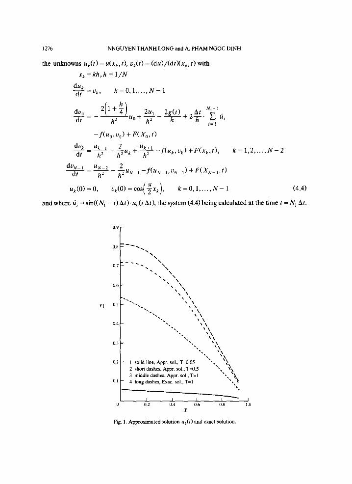
uk(0) = 0, vk(0) = cos ~ -x k , k = 0, 1 . . . . . N - 1 (4 .4)

and where fii = sin((N1 - i) At ) . Uo(i At), the system (4.4) being calculated at the t ime t = N 1 At.

0.9

0.8

(1.7

0.6

Y1 o.5

(1.4

0.3

0.2

O.l

,% \

• \ • \

• \ \

x \

x \ x \

x \ s \ " " " " " " - . x\x \

x \

1 solid line, Appr. sol., T=0.05 " ' " , ~ . k 2 short dashes, Appr. sol., T=0.5 - x~ 3 middle dashes, Appr. sol., T=I , , 4 long dashes, Exac. sol., T=I " • ~

I I I [ (1.2 0.4 0.6 0.8

X

Fig. 1. Approximated solution uk(t) and exact solution.

I 1 . 0

S e m i l i n e a r wave equation 1277

To solve the nonlinear differential system (4.4), we use the scheme generated by the nonlinear term

du(~ ") dt =v(k")' k = 0 , 1 , . . . , N - 1

[ h i dv (") 211 + ~-] u(0,) 2u~ ") 2 g ( t )

dt h 2 + h ~ h

U(n) k+ dvk (n) U(kn-)l 2 u(kn ) ~ -

d t h 2 h 2 + h 2

d,,(") U~)I ~N- 1

dt h z

u~") (o) = o,

following linear recursive

N 1 - 1

At fi}.) _ - - + 2 - h - " ]~ -f(u(o " l ) ,v(o"-O)+f(Xo,t ) i=1

f(u(k,- 1), V(k n - 1)) + F()Ck, t),

2 u(,, ) _f(u(~S~), o(n_ll)) + F ( X N 1,t) h 2 N-1

v(k ") (0) = cos -~x k , k = 0, 1 . . . . . N - 1

and where fi~") = sin ((Na - i) At). u(0 ") (i At).

k = l , 2 . . . . . N - 2

(4.5)

0.4

YI

0.3

0,2

0.1

0

-ILl

-0.2

-0.3

I I I

I I I I

-- I IIIII /

1 solid line = first case t / 2 short dashes = second case / /

I . I I I I I I I I I 0.1 1).2 0 .3 0 . 4 0 .5 0 .6 0 .7 0 .8 0 .9 1.0

T

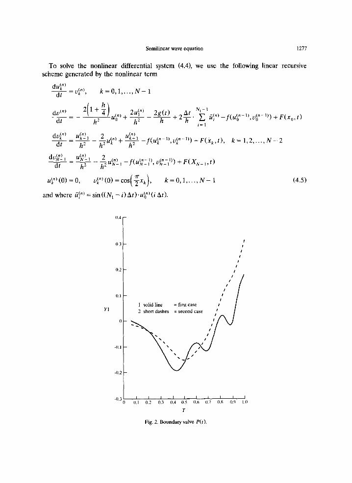
Fig. 2. Boundary valve P(t).


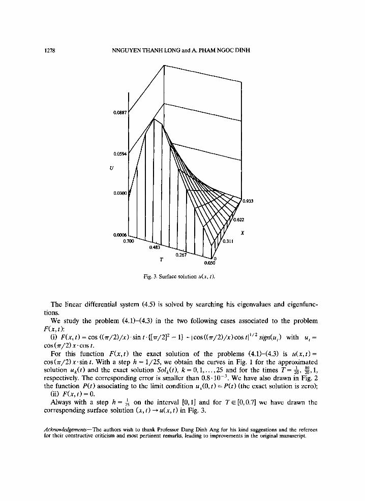
0.0887 ~ /

U °°594

0.0300[ I I .933

0.483 ""

T 0.050

Fig. 3. Surface solution u(x, t),

The linear differential system (4.5) is solved by searching his eigenvalues and eigenfunctions.

We study the problem (4.1)-(4.3) in the two following cases associated to the problem F(x , / ) :

(i) F(x , t) = cos ( (~r /2) /x) . sin t. {[zr/2] 2 - 1} + [cos ( ( z r /2 ) /x ) cos t l 1/2 sign(u t) with u t = cos (7r/2) x. cos t.

For this function F ( x , t ) the exact solution of the problems (4.1)-(4.3) is u ( x , t ) = cos(~- /2)x .s in t. With a step h = 1/25, we obtain the curves in Fig. 1 for the approximated solution uk(t) and the exact solution Solk(t), k = 0, 1 . . . . . 25 and for the times T = 1 10 ~ , ~ , 1, respectively. The corresponding error is smaller than 0.8-10 -3. We have also drawn in Fig. 2 the function P(t ) associating to the limit condition ux(O, t) = P( t ) (the exact solution is zero);

(ii) F(x , t) = O. 1 Always with a step h = ~ on the interval [0, 1] and for T ~ [0,0.7] we have drawn the

corresponding surface solution (x, t) ~ u(x, t) in Fig. 3.

Acknowledgements--The authors wish to thank Professor Dang Dinh Ang for his kind suggestions and the referees for their constructive criticism and most pertinent remarks, leading to improvements in the original manuscript.


R E F E R E N C E S

1. NGUYEN THUC AN & NGUYEN DINH TRIEU, Shock between absolutely solid body and elastic bar with the elastic viscous frictional resistance at the side, J. Mech. NCSR Vietnam Tom XIII(2),1-7 (1991).

2. DANG DINH ANG & PHAM NGOC DINH A., Mixed problem for some semilinear wave equation with a nonhomogeneous condition, Nonlinear Analysis 12, 581-592 (1988).

3. NGUYEN THANH LONG & PHAM NGOC DINH A., On the quasilinear wave equation: utt - Au + f (u , u t) = 0 associated with a mixed nonhomogeneous condition, Nonlinear Analysis 19, 613-623 (1992).

4. LAKSHMIKANTHAM V. & LEELA S., Differential and Integral Inequalities, Vol. 1. Academic Press, New York (1969).

5. LIONS J.-L., Quelques m~thodes de r~solution des problbmes aux lirnites nonlin(aires. Dunod-Gauthier-Villars, Paris (1969).

A semilinear wave equation associated with a linear differential equation with Cauchy data

Documents