A semi-nonparametric Poisson regression model for analyzing motor vehicle crash data Xin Ye 1 , Ke Wang 1 , Yajie Zou 1* , Dominique Lord 2 1 Key Laboratory of Road and Traffic Engineering of Ministry of Education, College of Transportation Engineering, Tongji University, Shanghai, China 2 Zachry Department of Civil Engineering Texas A&M University 3136 TAMU, College Station, TX, USA * Corresponding author Email: [email protected] (YZ)

Welcome message from author
This document is posted to help you gain knowledge. Please leave a comment to let me know what you think about it! Share it to your friends and learn new things together.
Transcript
A semi-nonparametric Poisson regression model for analyzing
motor vehicle crash data
Xin Ye1, Ke Wang1, Yajie Zou1*, Dominique Lord2
1Key Laboratory of Road and Traffic Engineering of Ministry of Education,
College of Transportation Engineering, Tongji University, Shanghai, China
2 Zachry Department of Civil Engineering
Texas A&M University 3136 TAMU, College Station, TX, USA
* Corresponding author
Email: [email protected] (YZ)
Abstract
This paper develops a semi-nonparametric Poisson regression model to analyze motor vehicle
crash frequency data collected from rural multilane highway segments in California, US. Motor
vehicle crash frequency on rural highway is a topic of interest in the area of transportation safety
due to higher driving speeds and the resultant severity level. Unlike the traditional Negative
Binomial (NB) model, the semi-nonparametric Poisson regression model can accommodate an
unobserved heterogeneity following a highly flexible semi-nonparametric (SNP) distribution.
Simulation experiments are conducted to demonstrate that the SNP distribution can well mimic a
large family of distributions, including normal distributions, log-gamma distributions, bimodal and
trimodal distributions. Empirical estimation results show that such flexibility offered by the SNP
distribution can greatly improve model precision and the overall goodness-of-fit. The semi-
nonparametric distribution can provide a better understanding of crash data structure through its
ability to capture potential multimodality in the distribution of unobserved heterogeneity. When
estimated coefficients in empirical models are compared, SNP and NB models are found to have
a substantially different coefficient for the dummy variable indicating the lane width. The SNP
model with better statistical performance suggests that the NB model overestimates the effect of
lane width on crash frequency reduction by 83.1%.
Keywords: Semi-nonparametric Distribution, Poisson Regression Model, Crash Frequency
Analysis, Negative Binomial Model, Transportation, Roads, Maximum Likelihood Estimation,
Statistical methods.
1. Introduction
Statistical regression models are typically used in analyzing the likelihood and severity of vehicle
crashes. Recent review studies [1-4] have summarized the innovative models for examining the
impact of factors (e.g., traffic, roadway and vehicle characteristics, etc.) on the likelihood of a
crash and its resulting injury severity. Regarding observed crash counts, previous studies often
found that some crash data are likely to demonstrate heterogeneity. This heterogeneity in the crash
data can be explained as the unknown variation of the impact of explanatory variables on crash.
As discussed by Mannering, et al.[3], when the crash-related information is collected, some factors
affecting the likelihood and severity of the vehicle crash may not be available to the transportation
safety analysts (e.g., driver’s weight, height, roadway lighting type, etc.). And different kinds of
data have been applied to the safety analysis[5,6]. To date, various models have been introduced
to or developed for crash modeling analysis. For example, mixed-Poisson models[7-11], latent
class/Markov switching models[12-17], random parameter models[18-27].
Among these crash modeling methods, the most frequently used statistical method for
modeling crash count data is the Negative Binomial (NB, also known as Poisson-gamma) model.
The NB model has its inadequacy when describing certain types of crash data. The distribution
assumed in the probabilistic error term related to the mean of the Poisson variable can be restrictive
in terms of its ability to account for different types of heterogeneity across observations. In
econometric literature, the semi-nonparametric (SNP) distribution has been introduced [28]. The
SNP distribution is developed based on a squared Kth-order polynomial expansion which can
provide a smooth estimation of the distribution of the error term[29-33]. Previous studies [34-36]
have shown the flexibility of SNP distribution. Thus, the SNP distribution can be used to model
the probabilistic error term regarding the mean of the Poisson variable by transportation safety
analysts to analyze crash data with heterogeneity.
Due to the importance of the error term related to the mean of the Poisson variable in
transportation crash modeling, the objective of this study is to examine whether or not the Poisson-
SNP distribution can capture the heterogeneity characteristics of crash data. To achieve this
objective, crash data sets are simulated using different combinations of fixed regression parameters
describing the mean and dispersion levels. Based on the simulated datasets, the parameter and
distribution of the error term are estimated and compared to the true values. The simulation
analysis are conducted due to the following reason: when real crash data are analyzed, the true
values of regression parameters and the distribution of the error term are seldom known in practice.
In contrast, in a simulation, it is possible to generate crash data with known regression parameters
and an assumed distribution for error term. The simulation analysis have been adopted in some
previous transportation safety studies[7,11] to evaluate the performance of different estimators. To
complement outputs from simulation studies, crash data collected in California of USA are also
used to compare the estimation results between the Poisson-SNP model and NB model.
2. Modeling methodology
This section presents the modeling methodology adopted in this paper. First, the Poisson regression
model is presented using the log-gamma heterogeneity (i.e., the Negative Binomial regression
model). Although the focus of this paper is to develop a Poisson regression model for crash
frequency with unobserved heterogeneity following a semi-nonparametric (SNP) distribution, it
will be insightful to present this state-of-practice model for comparison.
2.1. Negative binomial (NB) regression model: Poisson regression
model with log-gamma heterogeneity
Count data models are most suited to modeling dependent variable y that constitutes a frequency
or “count.” The dependent variable can only take non-negative integer values. In this paper, y
represents crash frequency for road section . The expectation of y is assumed to be and the
count data model formulation is as follows:
ln λ x , (1)
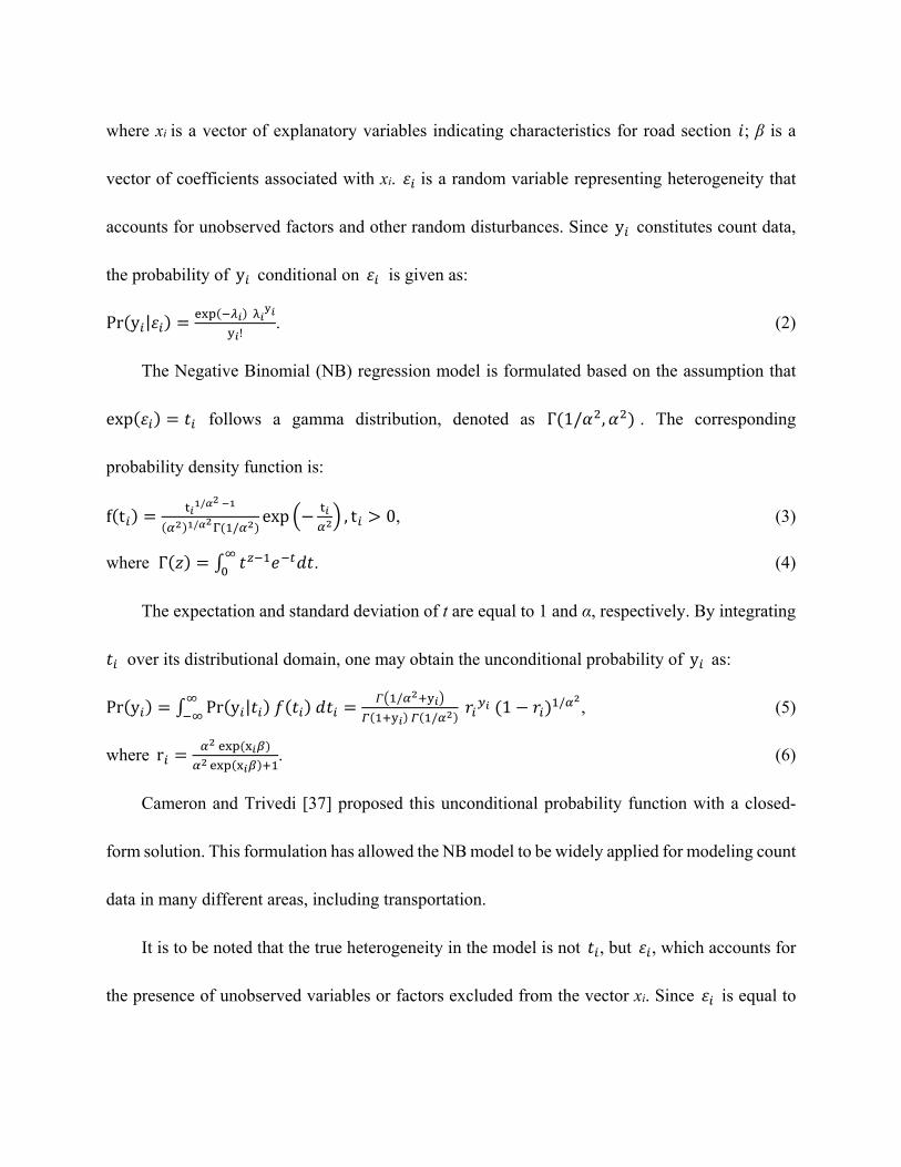
where xi is a vector of explanatory variables indicating characteristics for road section ; β is a
vector of coefficients associated with xi. is a random variable representing heterogeneity that
accounts for unobserved factors and other random disturbances. Since y constitutes count data,
the probability of y conditional on is given as:
Pr y |
!. (2)
The Negative Binomial (NB) regression model is formulated based on the assumption that
exp follows a gamma distribution, denoted as Γ 1/ , . The corresponding
probability density function is:
f t/
/ /exp , t 0, (3)
where Γ . (4)
The expectation and standard deviation of t are equal to 1 and α, respectively. By integrating
over its distributional domain, one may obtain the unconditional probability of y as:
Pr y Pr y | /
/ 1 / , (5)
where r . (6)
Cameron and Trivedi [37] proposed this unconditional probability function with a closed-
form solution. This formulation has allowed the NB model to be widely applied for modeling count
data in many different areas, including transportation.
It is to be noted that the true heterogeneity in the model is not , but , which accounts for
the presence of unobserved variables or factors excluded from the vector xi. Since is equal to
ln , the underlying distributional assumption on is the log-gamma distribution and the
probability density function can be derived as:
f/
exp ln , ∞ ∞. (7)
It is not a symmetric function with respect to the variable , indicating that the distribution
of the random variable is asymmetric in nature[38].
2.2. Poisson regression with SNP heterogeneity
To improve the flexibility of the distribution for unobserved heterogeneity, one may choose to use
the SNP distribution for representing heterogeneity . The probability density function for the
SNP distribution is usually specified as:
f ε∑
∑
. (8)
In Equation (8), "K" is the length of the polynomial, "m" is an index increasing from 0 to "K",
am is a constant coefficient, and φ ε represents the probability density function (PDF) of the
standard normal distribution. The denominator ensures that f ε dε 1. The denominator in
Equation (8) can be extended and written in the following form, where "n" is another index
increasing from 0 to "K":
∑ a ε φ ε dε
∑ ∑ a a ε φ ε dε (9)
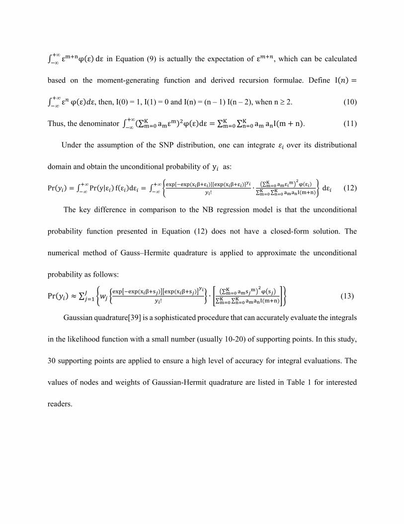
ε φ ε dε in Equation (9) is actually the expectation of ε , which can be calculated
based on the moment-generating function and derived recursion formulae. Define I
ε φ ε ε, then, I(0) = 1, I(1) = 0 and I(n) = (n – 1) I(n – 2), when n 2. (10)
Thus, the denominator ∑ a ε φ ε dε
∑ ∑ a a I m n . (11)
Under the assumption of the SNP distribution, one can integrate over its distributional
domain and obtain the unconditional probability of y as:
Pr Pr y|ε f ε dε
!∙
∑
∑ ∑
dε (12)
The key difference in comparison to the NB regression model is that the unconditional
probability function presented in Equation (12) does not have a closed-form solution. The
numerical method of Gauss–Hermite quadrature is applied to approximate the unconditional
probability as follows:
Pr ∑
!∙
∑
∑ ∑ (13)
Gaussian quadrature[39] is a sophisticated procedure that can accurately evaluate the integrals
in the likelihood function with a small number (usually 10-20) of supporting points. In this study,
30 supporting points are applied to ensure a high level of accuracy for integral evaluations. The
values of nodes and weights of Gaussian-Hermit quadrature are listed in Table 1 for interested
readers.
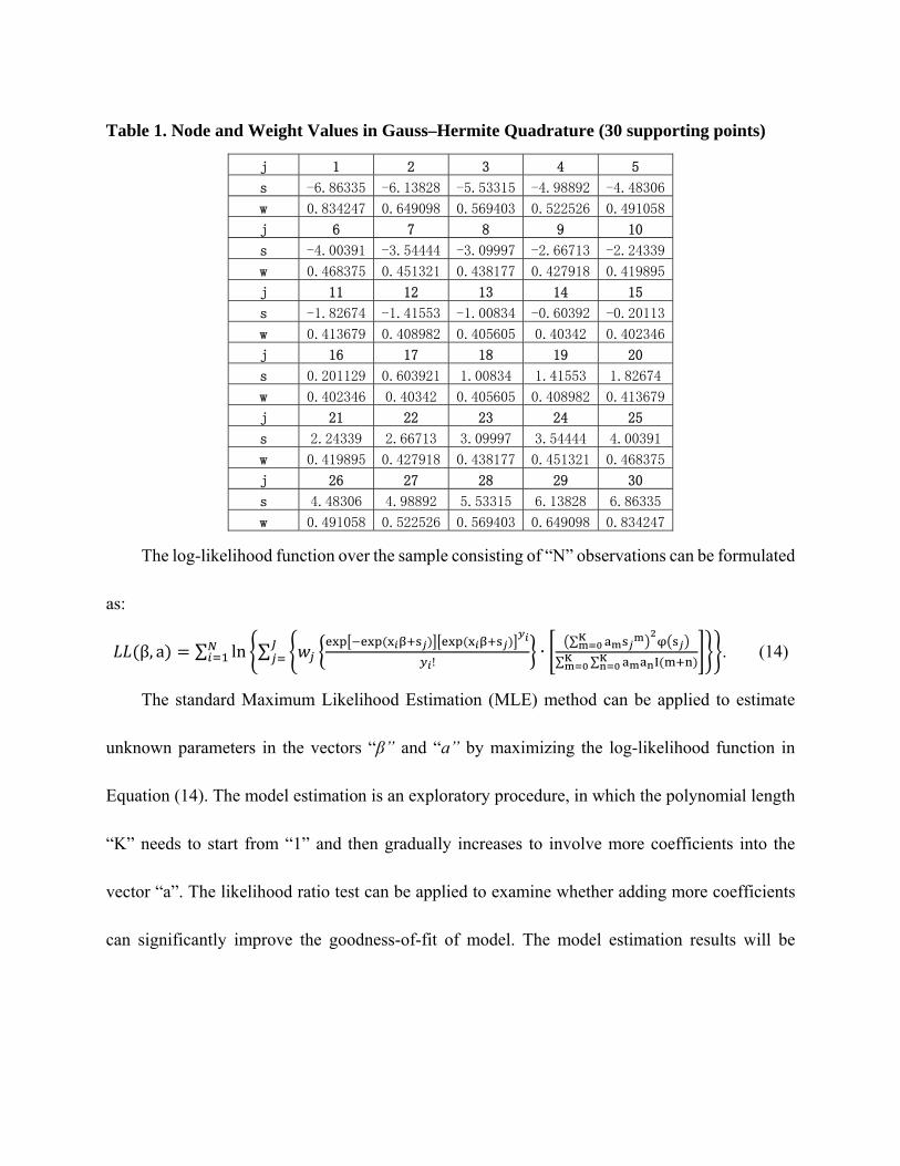
Table 1. Node and Weight Values in Gauss–Hermite Quadrature (30 supporting points)
j 1 2 3 4 5
s -6.86335 -6.13828 -5.53315 -4.98892 -4.48306
w 0.834247 0.649098 0.569403 0.522526 0.491058
j 6 7 8 9 10
s -4.00391 -3.54444 -3.09997 -2.66713 -2.24339
w 0.468375 0.451321 0.438177 0.427918 0.419895
j 11 12 13 14 15
s -1.82674 -1.41553 -1.00834 -0.60392 -0.20113
w 0.413679 0.408982 0.405605 0.40342 0.402346
j 16 17 18 19 20
s 0.201129 0.603921 1.00834 1.41553 1.82674
w 0.402346 0.40342 0.405605 0.408982 0.413679
j 21 22 23 24 25
s 2.24339 2.66713 3.09997 3.54444 4.00391
w 0.419895 0.427918 0.438177 0.451321 0.468375
j 26 27 28 29 30
s 4.48306 4.98892 5.53315 6.13828 6.86335
w 0.491058 0.522526 0.569403 0.649098 0.834247
The log-likelihood function over the sample consisting of “N” observations can be formulated
as:
β, a ∑ ln ∑
!∙
∑
∑ ∑. (14)
The standard Maximum Likelihood Estimation (MLE) method can be applied to estimate
unknown parameters in the vectors “β” and “a” by maximizing the log-likelihood function in
Equation (14). The model estimation is an exploratory procedure, in which the polynomial length
“K” needs to start from “1” and then gradually increases to involve more coefficients into the
vector “a”. The likelihood ratio test can be applied to examine whether adding more coefficients
can significantly improve the goodness-of-fit of model. The model estimation results will be
finalized when adding more coefficients fails to significantly improve the goodness-of-fit (GOF)
measure.
3. Simulation experiments
In this section, a number of simulation experiments are conducted to demonstrate the capability of
the SNP distribution to approximate different types of distributions for unobserved heterogeneities
in Poisson regression models. Those distributions include log-gamma distributions, normal
distributions, a bimodal distribution and a trimodal distribution.
3.1 SNP model approximating NB model (Poisson model with log-
gamma heterogeneity)
The NB model is the most practical modeling approach for crash frequency. It will be insightful
to examine whether an SNP distribution can well approximate the log-gamma heterogeneity in NB
models. The simulation experiments are designed as below:
λ exp 1.0 0.3 ∙ x1 0.4 ∙ x2 ,
where “x1” and “x2” independently follow a uniform distribution between 0 and 5; “ε” represents
the unobserved heterogeneity following the log-gamma distribution, whose PDF is given in
Equation (7) and the parameter 0.8. Then, the count variable “y” is drawn from a Poisson
distribution associated with the parameter λ
The sample size is setup at 1000. Based on the random sample consisting of the dependent variable
“y” and explanatory variables “x1” and “x2”, an NB model can be estimated and shown in the left
part of Table 2. As expected, the model coefficients are highly consistent with their true values.
With the same sample, an SNP model can be estimated as well and the estimation results are
presented in the right part of Table 2 for comparison. It should be noted that the coefficient a0
needs to be fixed at 1 for identification. The high flexibility of the SNP distribution causes that the
intercept in a regression model and the expectation of “ε” may not be simultaneously identifiable.
To solve this issue and facilitate comparisons, the intercept of the SNP model is fixed at the value
of intercept in the NB model.
Table 2. Comparison between NB and SNP Models ( = 0.8, Sample Size = 1000)
NB Model SNP Model
Variable
(True Value)
Value SE Value SE
b0 (1.0) 1.0031 0.0908 1.0031 --
b1 (-0.3) -0.2969 0.0239 -0.2969 0.0232
b2 (0.4) 0.3829 0.0243 0.3864 0.0244
(0.8) 0.8113 0.0541 -- --
a0 -- -- 1.0000 --
a1 -- -- -0.0581 0.0692
a2 -- -- -0.1393 0.0388
a3 -- -- -0.0521 0.0135
a4 -- -- 0.0207 0.0065
LL(β) -2372.46 -2372.61
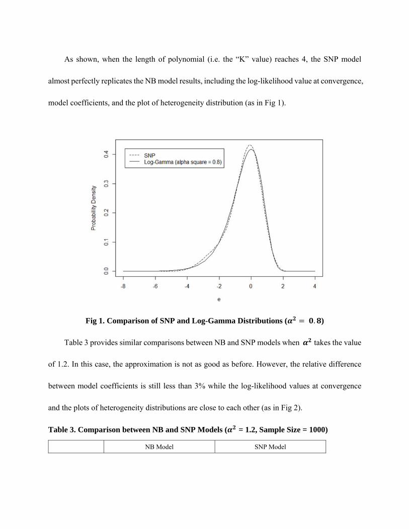
As shown, when the length of polynomial (i.e. the “K” value) reaches 4, the SNP model
almost perfectly replicates the NB model results, including the log-likelihood value at convergence,
model coefficients, and the plot of heterogeneity distribution (as in Fig 1).
Fig 1. Comparison of SNP and Log-Gamma Distributions ( . )
Table 3 provides similar comparisons between NB and SNP models when takes the value
of 1.2. In this case, the approximation is not as good as before. However, the relative difference
between model coefficients is still less than 3% while the log-likelihood values at convergence
and the plots of heterogeneity distributions are close to each other (as in Fig 2).
Table 3. Comparison between NB and SNP Models ( = 1.2, Sample Size = 1000)
NB Model SNP Model
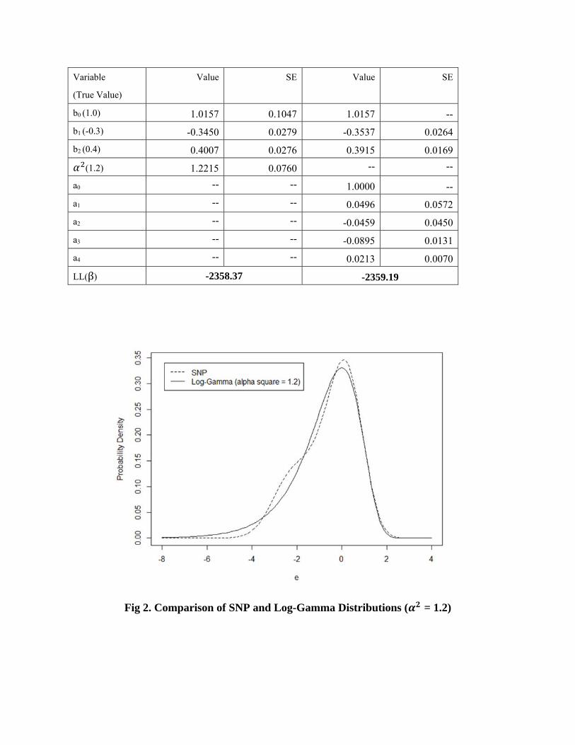
Variable
(True Value)
Value SE Value SE
b0 (1.0) 1.0157 0.1047 1.0157 --
b1 (-0.3) -0.3450 0.0279 -0.3537 0.0264
b2 (0.4) 0.4007 0.0276 0.3915 0.0169
(1.2) 1.2215 0.0760 -- --
a0 -- -- 1.0000 --
a1 -- -- 0.0496 0.0572
a2 -- -- -0.0459 0.0450
a3 -- -- -0.0895 0.0131
a4 -- -- 0.0213 0.0070
LL(β) -2358.37 -2359.19
Fig 2. Comparison of SNP and Log-Gamma Distributions ( = 1.2)
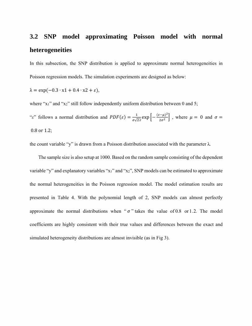
3.2 SNP model approximating Poisson model with normal
heterogeneities
In this subsection, the SNP distribution is applied to approximate normal heterogeneities in
Poisson regression models. The simulation experiments are designed as below:
λ exp 0.3 ∙ x1 0.4 ∙ x2 ,
where “x1” and “x2” still follow independently uniform distribution between 0 and 5;
“ε” follows a normal distribution and √
exp , where 0 and
0.8or1.2;
the count variable “y” is drawn from a Poisson distribution associated with the parameter λ
The sample size is also setup at 1000. Based on the random sample consisting of the dependent
variable “y” and explanatory variables “x1” and “x2”, SNP models can be estimated to approximate
the normal heterogeneities in the Poisson regression model. The model estimation results are
presented in Table 4. With the polynomial length of 2, SNP models can almost perfectly
approximate the normal distributions when “ ”takes the value of orThe model
coefficients are highly consistent with their true values and differences between the exact and
simulated heterogeneity distributions are almost invisible (as in Fig 3).
Table 4. SNP Models to Approximate Normal Heterogeneities (Sample Size = 1000)
SNP Model 1 ( ) SNP Model 2 ( )
Variable (True Value) Value SE Value SE
b1 (-0.3) -0.2993 0.0113 -0.3042 0.0151
b2 (0.4) 0.4090 0.0039 0.3946 0.0045
a0 1.0000 -- 1.0000 --
a1 0.0059 0.0332 0.0067 0.0305
a2 -0.1194 0.0185 0.0980 0.0218
LL(β) -2112.09 -2462.97
Fig 3. Comparison of SNP and Normal Distributions ( = 0.8 or 1.2)
3.3 SNP model approximating bimodal and trimodal distributions
This subsection further exhibits the great flexibility of the SNP distribution to approximate a
bimodal distribution and a trimodal distribution. The simulation experiments are designed as below:
λ exp 0.3 ∙ x1 0.4 ∙ x2 ,
where “x1” and “x2” still follow independently uniform distribution between 0 and 5. The
unobserved heterogeneity ε 3 ∙ D u 0.4 1.5 ∙ u 0.5 ∙ η 2.5 , where D( ) is an
indicator function, “ ” follows the standard normal distribution while “u1” and “u2” independently
follow the standard uniform distribution. The sample size is setup at 500. Since it is challenging
to derive the analytical PDF of the mixture distribution for the random variable “ε”, Kernel Density
Estimation (KDE) approach is employed to estimate density for each e in the arithmetic sequence
(e = -6.0, -5.9, … 5.9, 6.0) based on the random sample and following equation:
f e ∑ K e /500. (15)
In the formula, K u u/h /h. Namely, the PDF of standard normal distribution is
chosen as the smooth function K u and the bandwidth “h” is setup at 0.3. The estimated
probability density is plotted as a solid curve in Fig 4. As shown, it is a typical bimodal distribution
with two explicit modal points.
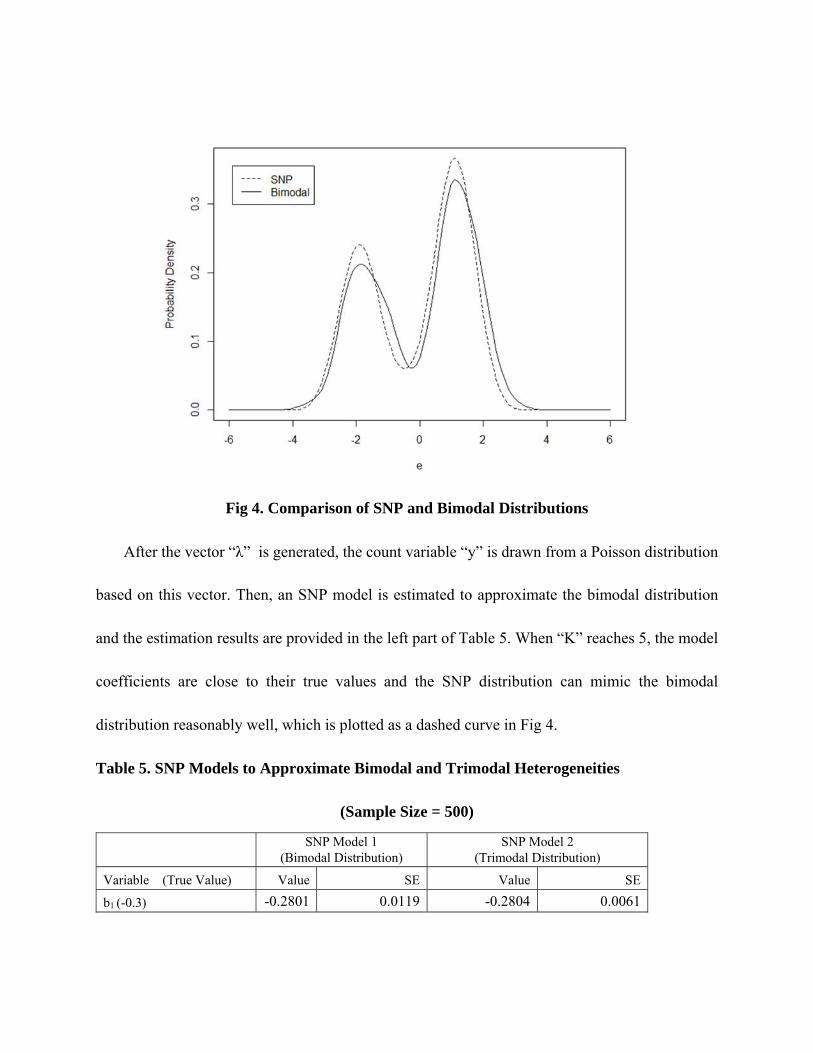
Fig 4. Comparison of SNP and Bimodal Distributions
After the vector “λ”is generated, the count variable “y” is drawn from a Poisson distribution
based on this vector. Then, an SNP model is estimated to approximate the bimodal distribution
and the estimation results are provided in the left part of Table 5. When “K” reaches 5, the model
coefficients are close to their true values and the SNP distribution can mimic the bimodal
distribution reasonably well, which is plotted as a dashed curve in Fig 4.
Table 5. SNP Models to Approximate Bimodal and Trimodal Heterogeneities
(Sample Size = 500)
SNP Model 1 (Bimodal Distribution)
SNP Model 2 (Trimodal Distribution)
Variable (True Value) Value SE Value SE
b1 (-0.3) -0.2801 0.0119 -0.2804 0.0061
b2 (0.4) 0.4139 0.0051 0.4107 0.0021
a0 1.0000 -- 1.0000 --
a1 0.8984 0.2587 -0.0496 0.0942
a2 0.9218 0.3554 -0.2594 0.0712
a3 -0.3543 0.1535 -0.0160 0.0514
a4 -0.0637 0.0485 0.0804 0.0088
a5 0.0174 0.0170 -0.0007 0.0047
LL(β) -1289.46 -1327.89
A last experiment is conducted to mimic a trimodal distribution. The unobserved
heterogeneity ε = 3 ∙ D(u1 > 0.8) – 3 · D(u2 > 0.7) + 2 ∙u3 + 0.5 ∙ – 1.0, where “ ” follows the
standard normal distribution while “u1” , “u2” and “u3” independently follow the standard uniform
distribution. The KDE approach is applied to estimate kernel densities using a bandwidth of 0.4
for better smoothness. The estimated distribution is then plotted as a solid curve in Fig 5. The
model coefficients, which are close to their true values, are presented in the right part of Table 5.
The dashed line in Fig 5 represents the SNP distribution mimicking the trimodal distribution. As
shown, the SNP distribution correctly exhibits the feature of the trimodal distribution with three
modal points and mimics the overall distribution reasonably well.
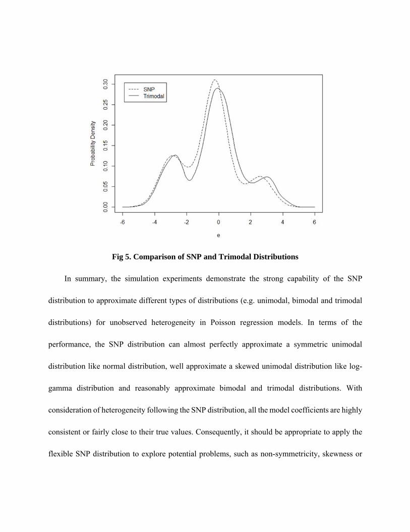
Fig 5. Comparison of SNP and Trimodal Distributions
In summary, the simulation experiments demonstrate the strong capability of the SNP
distribution to approximate different types of distributions (e.g. unimodal, bimodal and trimodal
distributions) for unobserved heterogeneity in Poisson regression models. In terms of the
performance, the SNP distribution can almost perfectly approximate a symmetric unimodal
distribution like normal distribution, well approximate a skewed unimodal distribution like log-
gamma distribution and reasonably approximate bimodal and trimodal distributions. With
consideration of heterogeneity following the SNP distribution, all the model coefficients are highly
consistent or fairly close to their true values. Consequently, it should be appropriate to apply the
flexible SNP distribution to explore potential problems, such as non-symmetricity, skewness or
multimodality, etc., in the distribution of the unobserved heterogeneities within a Poisson
regression model.
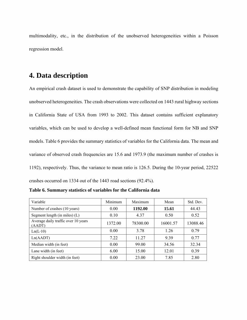
4. Data description
An empirical crash dataset is used to demonstrate the capability of SNP distribution in modeling
unobserved heterogeneities. The crash observations were collected on 1443 rural highway sections
in California State of USA from 1993 to 2002. This dataset contains sufficient explanatory
variables, which can be used to develop a well-defined mean functional form for NB and SNP
models. Table 6 provides the summary statistics of variables for the California data. The mean and
variance of observed crash frequencies are 15.6 and 1973.9 (the maximum number of crashes is
1192), respectively. Thus, the variance to mean ratio is 126.5. During the 10-year period, 22522
crashes occurred on 1334 out of the 1443 road sections (92.4%).
Table 6. Summary statistics of variables for the California data
Variable Minimum Maximum Mean Std. Dev.
Number of crashes (10 years) 0.00 1192.00 15.61 44.43
Segment length (in miles) (L) 0.10 4.37 0.50 0.52 Average daily traffic over 10 years (AADT) 1372.00 78300.00 16001.57 13088.46
Ln(L∙10) 0.00 3.78 1.26 0.79
Ln(AADT) 7.22 11.27 9.39 0.77
Median width (in feet) 0.00 99.00 34.56 32.34
Lane width (in feet) 6.00 15.00 12.01 0.39
Right shoulder width (in feet) 0.00 23.00 7.85 2.80
5. Empirical estimation results
This section presents the comparison results between the NB and SNP models. Table 7
presents all the estimate results and overall performance measurements of both NB model and SNP
model of crash frequency for comparisons. In the SNP model, the log-likelihood value at
convergence can be gradually improved until the polynomial length “K” reaches 3. The
performance measurements are listed at the bottom of the table, including the log-likelihood value
at convergence [i.e. LL( β )], Deviance, Akaike information criterion (AIC) and Bayesian
information criterion (BIC). The following formulae are used to compute those performance
measurements:
Deviance = – 2 ∙LL(β),
AIC = 2 ∙k – 2 ∙LL(β),
BIC = ln(n)∙k – 2∙LL(β),
where “n” represents the sample size and “k” represents the number of parameters estimated in the
model. A greater value in LL(β) or a less value in Deviance indicates a better goodness-of-fit (GOF)
for the data.

Table 7. Crash Frequency Model Estimation Results
NB Model SNP Model
Variable Value SE Value SE
Intercept -7.0561 0.6873 -7.0561 --.
Ln[10×length] 1.0000 -- 1.0000 --.
Ln(AADT) 1.0711 0.0267 1.0046 0.0187
Median -0.0348 0.0083 -0.0369 0.0056
Lane -0.1266 0.0542 -0.0677 0.0171
Right shoulder width (ft) -0.0733 0.0093 -0.0699 0.0043
α 0.5035 0.0239 -- --
a0 -- -- 1.0000 --
a1 -- -- -0.3242 0.0336
a2 -- -- -0.1714 0.0164
a3 -- -- 0.0408 0.0093
Overall Performance Measurements
Sample size 1443 1443
LL(β) -4480.06 -4441.44
Deviance 8960.13 8882.87
AIC 8972.13 8896.87
BIC 9003.78 8933.79
As shown in Table 7, the SNP model greatly improves the GOF for the data relative to the
NB model after 3 additional parameters for the SNP distribution are specified into the model. AIC
and BIC are two alternative criteria for model selection by penalizing the number of parameters in
models and avoiding overfitting issues. A smaller value of AIC or BIC indicates a better
performance of the SNP model than that of the NB model. It implies that it is worth specifying
additional coefficients to better describe the distribution of the unobserved heterogeneity and
further improve the model performance. In addition, the Chi-squared test is applied to examine
whether adding more coefficients can significantly improve the goodness-of-fit of the SNP model.
When the polynomial length “K” reaches 3, the Chi-squared test value is 164.36 relative to the
log-likelihood value with “K” at 1 and the critical value is 5.99 for 2 degrees of freedom. Since
the increase of the polynomial length fails to further significantly improve the goodness-of-fit, the
model is finalized at the polynomial length of 3.
Fig 6 visualizes the SNP distribution and compares it with the estimated log-gamma
distribution in the NB model. It is interesting to see that the estimated SNP distribution exhibits
three visible modal points, although the left and right ones are fairly minor. They are presumed to
correspond to three groups of observations in the sample. The major one occurs near -0.3 on the
coordinate of “ε” and takes a density value of 0.56, corresponding to the largest group in the middle
of the distributional domain. This group consists of almost all the (about 99.5%) observations in
the sample. The left mode occurs near -3.3 on the coordinate and the relevant small group consists
of about 0.4% of all the observations. The right modal point occurs near +2.6 on the coordinate
and the relevant group only consists of 0.1% of observations. Since the heterogeneity “ε”
represents unobserved or unspecified factors affecting crash frequency, those results indicate the
existence of three groups of highway segments exposed to different levels of crash risk, which
may be denoted as “low risk”, “medium risk” and “high risk” groups. About 6 (= 1443∙0.4%)
highway segments from the sample fall into the “low risk” group. If the expected crash frequencies
are compared between the “low risk” and “medium risk” groups, the expectation of “low risk” can
be only 5% of that of “medium risk” [i.e. exp 3.3 0.3 ] even if all the observed and specified
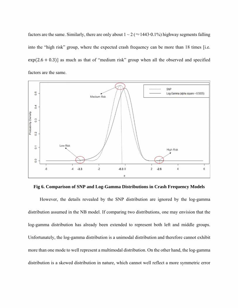
factors are the same. Similarly, there are only about 1 ~ 2 (≈1443∙0.1%) highway segments falling
into the “high risk” group, where the expected crash frequency can be more than 18 times [i.e.
exp 2.6 0.3 ] as much as that of “medium risk” group when all the observed and specified
factors are the same.
Fig 6. Comparison of SNP and Log-Gamma Distributions in Crash Frequency Models
However, the details revealed by the SNP distribution are ignored by the log-gamma
distribution assumed in the NB model. If comparing two distributions, one may envision that the
log-gamma distribution has already been extended to represent both left and middle groups.
Unfortunately, the log-gamma distribution is a unimodal distribution and therefore cannot exhibit
more than one mode to well represent a multimodal distribution. On the other hand, the log-gamma
distribution is a skewed distribution in nature, which cannot well reflect a more symmetric error
distribution of observations in the middle group. As a result, the GOF of the SNP model is much
better than that of the NB model thanks to its advantages to have multiple modes and represent a
more symmetric distribution.
In addition to the overall model performance, the SNP model brings great benefit to improve
the precision of model estimators. If comparing the standard errors of coefficient estimators
between SNP and NB models, one may see that some of them are reduced by a few times. As we
know, MLE estimators are consistent and efficient only if the distributional assumption is valid.
When the heterogeneity is well mimicked by the SNP distribution, the model coefficient estimators
have much less standard errors and are more precise than those in the NB model based on the
inappropriate unimodal and skewed distribution for unobserved heterogeneity. When comparing
magnitude of estimated coefficients, one may find that SNP and NB models have similar
coefficient estimators except that of the dummy variable indicating the lane width. The SNP model
with better statistical performance suggests that the NB model substantially overestimates the
effect of lane width on crash frequency reduction by 83.1% ( 1 exp 0.1266 v.s. 1
exp 0.0677 ). The striking difference is probably caused by a better representation of the error
distribution in the SNP model.
6. Conclusions and discussions
In this paper, the authors specify a semi-nonparametric (SNP) distribution to represent the
unobserved heterogeneity in a Poisson regression model for crash frequency analysis. Relative to
the unimodal log-gamma distribution in the conventional negative binomial model, the SNP
distribution is highly flexible to mimic different types of distributions. When the length of
polynomial increases, the SNP distribution can approximate a large family of distributions,
including symmetric or asymmetric unimodal distribution and different types of multimodal
distributions. Traffic crash analysts can take advantage of its flexibility to release distributional
restrictions imposed by the conventional modeling method and explore the most appropriate
distributional form for the unobserved heterogeneity.
In the empirical study based on the crash dataset collected from the California State of USA,
the SNP distribution classifies the observations from the sample into three groups, which are
exposed to different levels of risk. The SNP model fits data substantially better than the
conventional NB model and provides more precise model coefficient estimators. The NB model
is found to substantially overestimate the effect of lane width on crash frequency reduction relative
to the SNP model based on more robust estimation of unobserved heterogeneity.
Future research may be carried out in the following three directions. At first, an approach may be
required to classify observations into the groups identified by the SNP model. With this approach,
there may be great potential to identify “high-risk” and “low-risk” locations associated with
unobserved risk factors for further considerations. In addition, the crash model may be re-estimated
based on the observations belonging to the “medium-risk” group, where the unobserved
heterogeneity is more narrowly distributed. If it can be realized, the goodness-of-fit of the model
may be further improved, while all the model coefficients will reflect the situation with the most
“medium-risk” locations since “outliers” in “high-risk” and “low-risk” locations are omitted from
the sample. Second, the SNP model needs to be applied to some other crash frequency datasets to
further examine its applicability in different occasions. Third, there are different methods to
capture the heterogeneity. Instead of modifying the distribution of the random component , a
random parameter model can also be explored to capture the heterogeneity and improve the
goodness-of-fit of model. In future research, a random parameter model may be developed and
compared with the SNP model and the traditional NB model.
Reference 1. Lord D, Mannering F. The statistical analysis of crash-frequency data: a review and
assessment of methodological alternatives. Transportation Research Part A: Policy and Practice. 2010; 44: 291-305.
2. Mannering FL, Bhat CR. Analytic methods in accident research: Methodological frontier and future directions. Analytic methods in accident research. 2014; 1: 1-22.
3. Mannering FL, Shankar V, Bhat CR. Unobserved heterogeneity and the statistical analysis of highway accident data. Analytic methods in accident research. 2016; 11: 1-16.
4. Savolainen PT, Mannering FL, Lord D, Quddus MA. The statistical analysis of highway crash-injury severities: a review and assessment of methodological alternatives. Accident Analysis & Prevention. 2011; 43: 1666-1676.
5. Chen P, Yu G, Wu X, Ren Y, Li Y. Estimation of red-light running frequency using high-resolution traffic and signal data. Accident Analysis & Prevention. 2017; 102: 235-247.
6. Chen P, Zeng W, Yu G, Wang Y. Surrogate safety analysis of pedestrian-vehicle conflict at intersections using unmanned aerial vehicle videos. Journal of Advanced Transportation. 2017; 2017: Article ID 5202150.
7. Francis RA, Geedip.zally SR, Guikema SD, Dhavala SS, Lord D, LaRocca S. Characterizing the performance of the conway‐maxwell poisson generalized linear model. Risk Analysis. 2012; 32: 167-183.
8. Ma Z, Zhang H, Steven I, Chien J, Wang J, Dong C. Predicting expressway crash frequency using a random effect negative binomial model: A case study in China. Accident Analysis & Prevention. 2017; 98: 214-222.
9. Wang K, Ivan JN, Ravishanker N, Jackson E. Multivariate poisson lognormal modeling of crashes by type and severity on rural two lane highways. Accident Analysis & Prevention. 2017; 99: 6-19.
10. Ye X, Pendyala RM, Shankar V, Konduri KC. A simultaneous equations model of crash frequency by severity level for freeway sections. Accident Analysis & Prevention. 2013; 57: 140-149.
11. Zou Y, Wu L, Lord D. Modeling over-dispersed crash data with a long tail: examining the accuracy of the dispersion parameter in negative binomial models. Analytic Methods in Accident Research. 2015; 5: 1-16.
12. Eluru N, Bagheri M, Miranda-Moreno LF, Fu L. A latent class modeling approach for identifying vehicle driver injury severity factors at highway-railway crossings. Accident Analysis & Prevention. 2012; 47: 119-127.
13. Tang J, Liu F, Zou Y, Zhang W, Wang Y. An improved fuzzy neural network for traffic speed prediction considering periodic characteristic. IEEE Transactions on Intelligent Transportation Systems. 2017; 18: 2340-2350.
14. Xiong Y, Tobias JL, Mannering FL. The analysis of vehicle crash injury-severity data: A Markov switching approach with road-segment heterogeneity. Transportation research part B: methodological. 2014; 67: 109-128.
15. Yasmin S, Eluru N, Bhat CR, Tay R. A latent segmentation based generalized ordered logit model to examine factors influencing driver injury severity. Analytic methods in accident research. 2014; 1: 23-38.
16. Zou Y, Yang H, Zhang Y, Tang J, Zhang W. Mixture modeling of freeway speed and headway data using multivariate skew-t distributions. Transportmetrica A: Transport Science. 2017; 13: 657-678.
17. Heydari S, Fu L, Miranda-Moreno LF, Joseph L. Using a flexible multivariate latent class approach to model correlated outcomes: A joint analysis of pedestrian and cyclist injuries. Analytic Methods in Accident Research. 2017; 13: 16-27.
18. Anastasopoulos PC, Mannering FL. An empirical assessment of fixed and random parameter logit models using crash-and non-crash-specific injury data. Accident Analysis & Prevention. 2011; 43: 1140-1147.
19. Buddhavarapu P, Scott JG, Prozzi JA. Modeling unobserved heterogeneity using finite mixture random parameters for spatially correlated discrete count data. Transportation Research Part B: Methodological. 2016; 91: 492-510.
20. Dong C, Clarke DB, Yan X, Khattak A, Huang B. Multivariate random-parameters zero-inflated negative binomial regression model: An application to estimate crash frequencies at intersections. Accident Analysis & Prevention. 2014; 70: 320-329.
21. Sarwar MT, Fountas G, Anastasopoulos PC. Simultaneous estimation of discrete outcome and continuous dependent variable equations: A bivariate random effects modeling approach with unrestricted instruments. Analytic Methods in Accident Research. 2017; 16: 23-34.
22. Anastasopoulos PC, Tarko AP, Mannering FL. Tobit analysis of vehicle accident rates on interstate highways. Accident Analysis & Prevention. 2008; 40: 768-775.
23. Geedipally SR, Lord D, Dhavala SS. The negative binomial-Lindley generalized linear model: Characteristics and application using crash data. Accident Analysis & Prevention. 2012; 45: 258-265.
24. Behnood A, Mannering F. The effect of passengers on driver-injury severities in single-vehicle crashes: A random parameters heterogeneity-in-means approach. Analytic Methods in Accident Research. 2017; 14: 41-53.
25. Behnood A, Mannering F. Determinants of bicyclist injury severities in bicycle-vehicle crashes: A random parameters approach with heterogeneity in means and variances. Analytic Methods in Accident Research. 2017; 16: 35-47.
26. Bhat CR, Astroza S, Lavieri PS. A new spatial and flexible multivariate random-coefficients model for the analysis of pedestrian injury counts by severity level. Analytic Methods in Accident Research. 2017; 16: 1-22.
27. Buddhavarapu P, Scott JG, Prozzi JA. Modeling unobserved heterogeneity using finite mixture random parameters for spatially correlated discrete count data. Transportation Research Part B Methodological. 2016; 91: 492-510.
28. Gallant AR, Nychka DW. Semi-nonparametric maximum likelihood estimation. Econometrica: Journal of the Econometric Society. 1987: 363-390.
29. Gurmu S, Rilstone P, Stern S. Semiparametric estimation of count regression models1. Journal of Econometrics. 1999; 88: 123-150.
30. Tang J, Zhang S, Chen X, Liu F, Zou Y. Taxi trips distribution modeling based on Entropy-Maximizing theory: A case study in Harbin city—China. Physica A: Statistical Mechanics and its Applications. 2018; 493: 430-443.
31. Wang K, Ye X, Pendyala RM, Zou Y. On the development of a semi-nonparametric
generalized multinomial logit model for travel-related choices. PloS one. 2017; 12:
e0186689.
32. Ye X, Garikapati VM, You D, Pendyala RM. A practical method to test the validity of the standard Gumbel distribution in logit-based multinomial choice models of travel behavior. Transportation Research Part B: Methodological. 2017; 106: 173-192.
33. Ye X, Pendyala RM (2009) A Probit-based Joint Discrete-continuous Model System: Analyzing the Relationship between Timing and Duration of Maintenance Activities. In: Transportation and Traffic Theory 2009: Golden Jubilee. pp 403-423
34. Boucher J-P, Guillen M. A semi-nonparametric approach to model panel count data. Communications in Statistics-Theory and Methods. 2011; 40: 622-634.
35. León Á, Mencía J, Sentana E. Parametric properties of semi-nonparametric distributions, with applications to option valuation. Journal of Business & Economic Statistics. 2009; 27: 176-192.
36. Tang J, Liu F, Zhang W, Ke R, Zou Y. Lane-changes prediction based on adaptive fuzzy neural network. Expert Systems with Applications. 2018; 91: 452-463.
37. Cameron AC, Trivedi PK. Econometric models based on count data. Comparisons and applications of some estimators and tests. Journal of applied econometrics. 1986; 1: 29-53.
38. Lawless JF. Inference in the generalized gamma and log gamma distributions. Technometrics. 1980; 22: 409-419.
39. Press WH, Teukolsky SA, Vetterling WT, Flannery BP (2007) Numerical Recipes 3rd Edition: The Art of Scientific Computing. Cambridge University Press.
Related Documents


