A semi-dependent decomposition approach to learn hierarchical classifiers

A semi-dependent decomposition approach to

learn hierarchical classifiers

J. Dıez a J.J. del Coz a,∗ and A. Bahamonde a

aArtificial Intelligence Center, University of Oviedo at Gijon,E33271 Gijon, Asturias, Spain

http://www.aic.uniovi.es/MLGroup

Abstract

In hierarchical classification, classes are arranged in a hierarchy represented by a treeor a forest, and each example is labeled with a set of classes located on paths fromroots to leaves or internal nodes. In other words, both multiple and partial paths areallowed. A straightforward approach to learn a hierarchical classifier, usually usedas a baseline method, consists in learning one binary classifier for each node of thehierarchy; the hierarchical classifier is then obtained using a top-down evaluationprocedure. The main drawback of this naıve approach is that these binary classifiersare constructed independently, when it is clear that there are dependencies betweenthem that are motivated by the hierarchy and the evaluation procedure employed. Inthis paper, we present a new decomposition method in which each node classifier isbuilt taking into account other classifiers, its descendants, and the loss function usedto measure the goodness of hierarchical classifiers. Following a bottom-up learningstrategy, the idea is to optimize the loss function at every subtree assuming thatall classifiers are known except the one at the root. Experimental results show thatthe proposed approach has accuracies comparable to state-of-the-art hierarchicalalgorithms and is better than the naıve baseline method described above. Moreover,the benefits of our proposal include the possibility of parallel implementations, aswell as the use of all available well-known techniques to tune binary classificationSVMs.

Key words: Hierarchical classification, Multi-label learning, Structured outputclassification, Cost-sensitive learning, Support Vector Machines

∗ Corresponding author. Phone: +34 985 18 2501, Fax: +34 985 18 2125Email addresses: [email protected] (J. Dıez), [email protected] (J.J.

del Coz), [email protected] (A. Bahamonde).

Preprint submitted to Pattern Recognition 17 June 2010

1 Introduction

Many real-world domains require automatic systems to organize objects intoknown taxonomies. For instance, a news website, or a news service in general,needs to classify the latest articles into sections and subsections of the site[1–6]. This learning task is usually called hierarchical classification. Althoughmost of its applications deal with textual information, there are other fields inwhich hierarchical classification can be useful. The authors of [7,8] describedan algorithm to classify speech data into a hierarchy of phonemes. A systemwas presented in [9] in which a robot can infer the similarity between differenttools using a learned taxonomy. Another interesting task is related to biologicalterms: the Gene Ontology [10] is a controlled vocabulary used to representmolecular biology concepts and is the standard for annotating genes/proteins.This task has recently been addressed using hierarchical classification [11,12].

Hierarchical classification differs from multiclass learning in that: i) the wholeset of classes has a hierarchical structure usually defined by a tree, and ii) eachobject must be labeled with a set of classes consistent with the hierarchy: ifan object belongs to a class, then it must belong to any of its ancestors. Inmulti-label learning tasks, see for instance [13,14], training examples belongto a subset of labels too, but the output space does not necessarily have anyhierarchical structure.

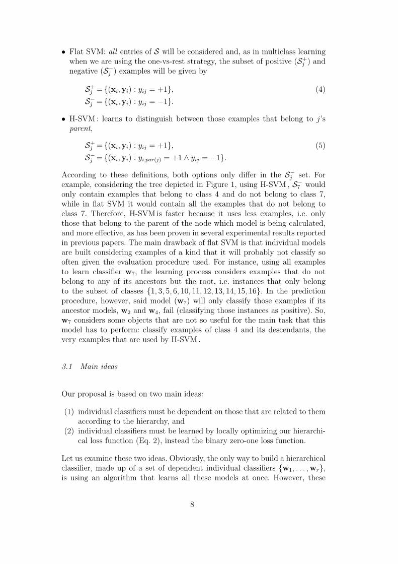
The aim of hierarchical classification algorithms is to learn a model that canaccurately predict a set of classes; notice that these subsets of classes generallyhave more than one element and are endowed with a subtree structure. Inthe more general case, see Figure 1, these subtrees may have more than onebranch (we then say that there are multipaths in the labels) and subtrees maynot end on a leaf (i.e. they include partial paths). In this paper we will presenta learning algorithm for hierarchical classification able to deal with multipleand partial paths.

1.1 Related work

As in multiclass classification, the algorithms available in the literature usedto solve hierarchical classification can be arranged into two main groups: thosethat take a decomposition approach, and those that learn a hierarchical classi-fier in a single process. Decomposition algorithms learn a model for each nodeof the hierarchy using different methods; a hierarchical classification of an ob-ject is then obtained by combining, in some way, the predictions of these in-dividual classifiers. The algorithms presented in [1–3,11] belong to this group.Hierarchical classification can, however, be seen as a whole rather than a series

2

1

2 3

4

8 97

5 6

13121110

161514

Fig. 1. Our approach can deal with examples that belong to multiple and partialpaths; for instance an example can belong to classes {1,2,4,3,6,12}.

of local learning tasks; the idea being to optimize the global performance allat once. This approach is adopted in [4–8].

In [1], Koller and Sahami employ a Bayesian classifier at each internal nodeof the hierarchy to distinguish between its children. In the learning stage,they only use those instances that belong to the class as training instances.Their approach does not permit multipath or partial paths in the labels: theexamples must belong to exactly one class at the bottom level of the hierarchyand the algorithm always predicts a single leaf.

In [2], a classifier is trained at each node and the outputs of all classifiers arecombined by integrating scores along each path. After training the supportvector machines (SVM) classifiers, the authors fit a sigmoid to the outputof the SVM using regularized maximum likelihood fitting. The SVM thusproduces posterior probabilities that are directly comparable across categories.

In [3], Cesa-Bianchi et al. presented an algorithm able to work with multi-paths and partial paths. Essentially it constructs a conditional regularizedleast squares estimator for each node. This is an on-line algorithm and in eachiteration an instance is presented to the current set of classifiers, the predictedlabels are compared to the true labels, and regularized least squares estimatorsare updated.

A two-step approach was presented in [11]: first, an SVM model is learned foreach node in an attempt to distinguish whether an instance belongs to thatnode, and then a Bayesian network is used to ensure that the predictions areconsistent with the hierarchy.

Cai and Hofmann [4,5] presented two algorithms based on the large marginprinciple. These authors also derive a novel taxonomy-based loss function be-tween overlapping categories that is motivated from real applications. The

3

difference between both papers is that in the former their algorithm is onlyable to predict one category, while in the latter, they employ the categoryranking approach proposed in [15] to deal with the additional challenge ofmultipaths.

In [6], Rousu et al. presented a kernel-based method in which the classifica-tion model is a variant of the maximum margin Markov network framework.This algorithm relies on a decomposition of the problem into single-examplesubproblems and conditional gradient ascent for optimisation of these sub-problems. They propose a loss function that decomposes into contributions ofedges so as to marginalize the exponential-sized problem into a polynomialone.

An on-line algorithm and a batch algorithm were presented in [7,8] combiningideas from large margin kernel methods and Bayesian analysis. The authorsassociate a prototype with each label in the hierarchy and formulate the learn-ing task as an optimization problem with varying margin constraints. Theyimpose similarity requirements between the prototypes corresponding to ad-jacent labels.

Finally, Vens et al. [16] compare three decision tree algorithms on the taskof hierarchical classification: i) an algorithm that learns a single tree thatpredicts all classes at once, ii) one that learns a separate decision tree for eachclass, and iii) an algorithm that learns and applies such single-label decisiontrees in a hierarchical way. The first one outperforms the others in all aspects:predictive performance, model size and efficiency.

1.2 Our approach

Some of the papers cited above, for instance [3,6], compare their methods withtwo baseline algorithms: a kind of ”flat” one-vs-rest multiclass SVM and a hi-erarchical classifier based on SVM, usually called H-SVM . Both algorithmsconsist in learning a binary classifier for each node (class) of the hierarchy topredict whether an example belongs to the class at that node or not. The dif-ference between both methods is that H-SVM constructs each binary classifierusing only training examples for which the ancestor labels are positive, whilemulticlass SVM uses all examples. In order to make a fair comparison withhierarchical approaches and to guarantee consistent predictions with respectto the hierarchy, in the prediction phase of both baseline algorithms, the set ofmodels are applied to an instance using a top-down evaluation procedure untila classifier fails to include that node in its predicted classes. This evaluationprocess also means that both algorithms are able to deal with multipath andpartial path predictions.

4

In the experimental results reported in the literature, H-SVM is very com-petitive with respect to the proposed hierarchical algorithms and outper-forms flat multiclass SVM. The only reason explaining the latter result isthat H-SVM employs the predefined hierarchy to select the training examplesused to build each SVM classifier. H-SVM takes into account the fact that,given the evaluation procedure used, the binary classifier of each node will beapplied after its ancestors.

However, the main drawback of H-SVM is that binary classifiers are still con-structed independently. As in multiclass classification, the advantage of di-rect methods over decomposition approaches is that the formers can capturesome dependencies between individual classifiers. In the context of hierarchi-cal classification, the presence of such dependencies is even clearer. They aremotivated by the hierarchy and, in the case of H-SVM , also by the evaluationprocedure.

In this paper, we shall present a new decomposition method that aims to im-prove the performance of H-SVM . Let us remark that H-SVM takes into ac-count the hierarchical dependencies between the classes to select the trainingexamples for each binary classifier. We want to exploit these dependencies evenmore. In our approach, binary classifiers are not independent: each node clas-sifier is learned considering the predictions of other classifiers, its descendants,and the loss function used to measure the goodness of hierarchical classifiers.Following a bottom-up learning strategy, the idea is to optimize the loss func-tion at every subtree assuming that all classifiers are known except the oneat the root. We shall show that the performance of the two baseline methodsdescribed in this section can be improved using this learning method. The aimis to prove that a decomposition approach for hierarchical classification canbe as successful as in multiclass classification [17].

In addition to the performance obtained, the advantages of decompositionalgorithms for hierarchical classification are derived from their modularity.They can be straightforwardly implemented in a parallel platform to obtaina very fast learning method. They are simple and can be built, with someeasy adaptations, with the user’s favorite binary classifier; for instance, SVM.Moreover, the overall performance of the classifier can be improved using well-known techniques available for tuning binary classifiers, as occurs with SVM.

1.3 Outline of the paper

The paper is organized as follows. The next section formally introduces hier-archical learning, including appropriate loss functions, and the notation usedthroughout the rest of the paper. The third section is devoted to explaining the

5

proposed decomposition method in detail. We present the main idea and showhow it can be easily implemented using cost-sensitive binary SVM. Finally,the last section reports some experiments on benchmark data sets conductedto compare the approach presented here with other state-of-the-art algorithmsin the context of hierarchical classification.

2 Hierarchical classification

In hierarchical classification, we have a set of classes arranged according toa known taxonomy. Formally, we have a tree T with r nodes, one for eachclass. In fact, we could start from a forest of trees F , but then we would addan artificial root node to join the whole set of classes in a tree. Therefore, inwhat follows, we shall consider our hierarchy to be represented by a tree T .In this context, hierarchical classification tasks are defined by a training setS = {(x1,y1), . . . , (xn,yn)}, in which each example is described by an entryrepresented by a vector xi of an input space X , and a vector yi of an outputspace Y ⊂ {−1,+1}r. We shall interpret each output yi as a subset of theset of classes {1, . . . , r}: yij = +1 if and only if the ith example belongs to thejth class. In the following, we shall use the symbol yi both as a vector andas a subset of classes when no confusion can arise. We shall assume that allelements of Y observe the underlying hierarchy defined by T in the sense that

∀yi ∈ Y , yij = −1⇒ ∀k ∈ des(j), yik = −1,

in which des(j) stands for the set of descendants of node or class j, but notincluding j.

A straightforward approach to learn tasks of this kind may consist in learninga family of binary models {w1, . . . ,wr}, one for each node (class) of T . Forinstance, using linear classifiers, an entry x will be assigned to all classes jsuch that (+1 = sign(〈wj,x〉)). However, this procedure may lead to incon-sistent predictions with respect to T . To avoid these, a top-down predictionprocedure can be used, as in [3,6]. Thus, an entry can only be assigned to aclass j if it was previously classified into its parent class, par(j); therefore, anentry not assigned to one class, will automatically not be assigned to any ofits descendants. This approach is followed, for instance, by the two baselinemethods described in Section 1.2.

2.1 Loss functions

To complete the specification of the hierarchical learning task, we need to de-cide which loss function will be used to measure the goodness of the hypothesis

6

learned. A first option may be to employ the zero-one loss function:

l0/1(yi,y′i) = [yi 6= y′i]. (1)

The problem is that it is not possible using this loss function to capture anydifference between very wrong predictions and nearly correct ones.

In a real-world application, hopefully, an expert in the field could provide uswith the costs of having false positives (fp(j)) and false negatives (fn(j)) foreach class j [4]. Then, we can define

lT (yi,y′i) =

∑j∈yi−y′i

fn(j) +∑

j∈y′i−yi

fp(j). (2)

Nevertheless, in the experiments reported below, as in [4–6], we always assumethat all costs have value 1, and so we obtain a loss function that only reflectsthe cardinality of the symmetric difference of a pair of subsets of classes: thenumber of different elements. In symbols:

l∆(yi,y′i) =

r∑j=1

[yij 6= y′ij] = |(y′i − yi) ∪ (yi − y′i)| = |y′i yi|. (3)

In [6], Rousu et al. proposed other loss functions, weighting the classes accord-ing to the proportion of the hierarchy that is in the subtree Tj rooted by nodej, or sharing the relevance of each node between its siblings starting with 1for the root. It is easy to see that these loss functions are particular cases ofthe general framework, lT , presented here.

3 A semi-dependent decomposition hierarchical classifier: H-SVM lT

We shall now describe our approach to build hierarchical learners based onthe use of binary classifiers and a straightforward implementation using SVM.Following the notation of the previous section, we assume that we have beforeus a learning task specified by a training set S and two real positive functions,fp and fn, to compute the costs of false positives and false negatives of classes,respectively.

The aim of this paper is to discover how to design a decomposition approachto learn a competitive hierarchical classifier, in the same way that decomposi-tion methods are used to successfully solve multiclass classification tasks. Ourgoal is to improve the performance of the two most popular decompositionalgorithms used as baseline methods in hierarchical classification papers: akind of flat SVM and H-SVM , see Section 1.2. Recall that the only differencebetween both methods is the set of examples used to learn each model wj.Formally,

7

• Flat SVM: all entries of S will be considered and, as in multiclass learningwhen we are using the one-vs-rest strategy, the subset of positive (S+

j ) andnegative (S−j ) examples will be given by

S+j = {(xi,yi) : yij = +1}, (4)

S−j = {(xi,yi) : yij = −1}.

• H-SVM : learns to distinguish between those examples that belong to j’sparent,

S+j = {(xi,yi) : yij = +1}, (5)

S−j = {(xi,yi) : yi,par(j) = +1 ∧ yij = −1}.

According to these definitions, both options only differ in the S−j set. Forexample, considering the tree depicted in Figure 1, using H-SVM , S−7 wouldonly contain examples that belong to class 4 and do not belong to class 7,while in flat SVM it would contain all the examples that do not belong toclass 7. Therefore, H-SVM is faster because it uses less examples, i.e. onlythose that belong to the parent of the node which model is being calculated,and more effective, as has been proven in several experimental results reportedin previous papers. The main drawback of flat SVM is that individual modelsare built considering examples of a kind that it will probably not classify sooften given the evaluation procedure used. For instance, using all examplesto learn classifier w7, the learning process considers examples that do notbelong to any of its ancestors but the root, i.e. instances that only belongto the subset of classes {1, 3, 5, 6, 10, 11, 12, 13, 14, 15, 16}. In the predictionprocedure, however, said model (w7) will only classify those examples if itsancestor models, w2 and w4, fail (classifying those instances as positive). So,w7 considers some objects that are not so useful for the main task that thismodel has to perform: classify examples of class 4 and its descendants, thevery examples that are used by H-SVM .

3.1 Main ideas

Our proposal is based on two main ideas:

(1) individual classifiers must be dependent on those that are related to themaccording to the hierarchy, and

(2) individual classifiers must be learned by locally optimizing our hierarchi-cal loss function (Eq. 2), instead the binary zero-one loss function.

Let us examine these two ideas. Obviously, the only way to build a hierarchicalclassifier, made up of a set of dependent individual classifiers {w1, . . . ,wr},is using an algorithm that learns all these models at once. However, these

8

methods present the disadvantage of their computational complexity, whichdepends on the number of classes. This number is usually much bigger in hier-archical classification tasks than in multiclass problems. We can significantlyreduce this complexity by following a decomposition approach, but we haveto pay a price: we cannot build each classifier depending on all others. Wehave to restrict ourselves to learn each classifier depending only on some ofthe others.

Given the hierarchy described by T , we basically have two options: each clas-sifier can depend on its ancestors, using a top-down learning strategy, or on itsdescendants, using a bottom-up algorithm. But it makes more sense for eachclassifier to depend on its descendants. The main reason is that, dependingon the top-down prediction procedure used to ensure hierarchically consistentresponses, parent models can change the predictions of their descendants:whenever they classify an example as negative, it is also classified as negativein all of their descendant classes. Therefore, a model has more influence onthe overall performance of the learner when it is closer to the root. Takinginto account these circumstances, it is preferable for models near to the rootto be computed later, using the information of their descendants: they canknow the predictions of their descendant models and use these predictions tobuild a classifier adapted to them, thus improving the overall performance ofthe local hierarchical learner placed at that subtree. Following this reasoning,our approach uses a bottom-up learning strategy, models are calculated fromleaf nodes to the root of the tree, and each classifier depends on the classifiersof its descendant classes.

The second idea is to change the loss function optimized to learn each individ-ual classifier. As in multiclass tasks, the individual classifiers of the proposedhierarchical decomposition methods optimize the binary zero-one loss func-tion. In hierarchical classification, however, this setting is not appropriate.Moreover, if we consider that in our approach each binary classifier wj willbe built when all other classifiers of the subtree rooted at node j (Tj) areknown, then we can optimize any hierarchical loss function instead the binaryzero-one loss function.

In fact both ideas are complementary: locally optimizing the hierarchical lossfunction described in Eq. 2 requires that the different subsets of binary clas-sifiers must be considered together. Combining both, our method is based onbuilding each binary classifier optimizing the hierarchical loss function used,and considering that all classifiers of the subtree rooted at that node have beenlearned before. Our experimental results will show that a better decompositionmethod can be obtained using this bottom-up learning procedure.

9

3.2 Using cost-sensitive learning to optimize lT at every subtree

To the best of our knowledge, all the new loss functions proposed to deal withhierarchical classification, including our proposal (Eq. 2), are example-basedfunctions, i.e., they decompose linearly into a combination of the individualclassification errors. In order to optimize such functions, we need only bear inmind that it will not be the same to classify each training example incorrectly;in other words, each example can make a different contribution to the overallloss. These are the kind of tasks that cost-sensitive learning methods [18]solve. Our approach is therefore based on assigning different costs to eachexample during learning; these costs depend on the hierarchy of classes, theloss function used and, as we shall see, the top-down prediction procedure.Before learning all our binary classifiers, we have to calculate the cost thateach example must have and then apply any binary cost-sensitive learner ableto assign different costs to each example.

In the trivial case, when we are learning a model wj of a leaf node j, forinstance w7 in the learning task depicted in Figure 1, the loss of each examplexi is

lT (yij, y′ij) =

0 if yij = y′ij,

fn(j) if yij = +1, y′ij = −1,

fp(j) if yij = −1, y′ij = +1,

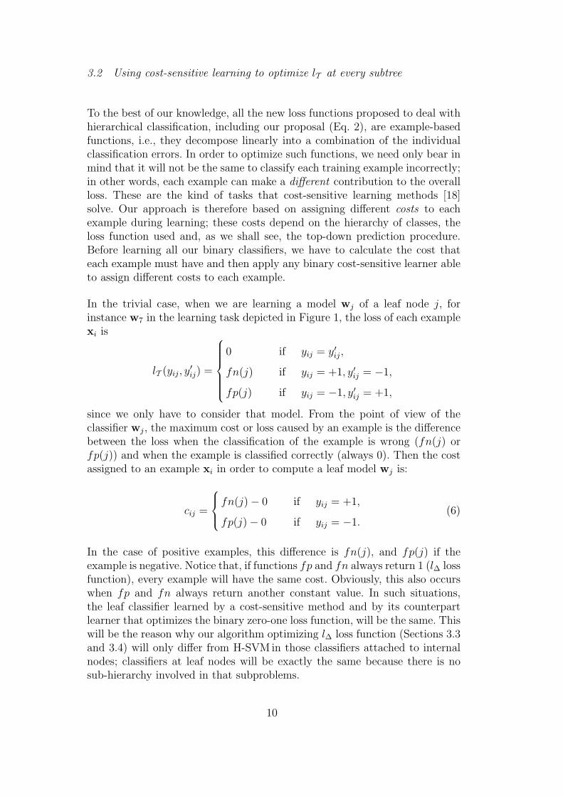
since we only have to consider that model. From the point of view of theclassifier wj, the maximum cost or loss caused by an example is the differencebetween the loss when the classification of the example is wrong (fn(j) orfp(j)) and when the example is classified correctly (always 0). Then the costassigned to an example xi in order to compute a leaf model wj is:

cij =

fn(j)− 0 if yij = +1,

fp(j)− 0 if yij = −1.(6)

In the case of positive examples, this difference is fn(j), and fp(j) if theexample is negative. Notice that, if functions fp and fn always return 1 (l∆ lossfunction), every example will have the same cost. Obviously, this also occurswhen fp and fn always return another constant value. In such situations,the leaf classifier learned by a cost-sensitive method and by its counterpartlearner that optimizes the binary zero-one loss function, will be the same. Thiswill be the reason why our algorithm optimizing l∆ loss function (Sections 3.3and 3.4) will only differ from H-SVM in those classifiers attached to internalnodes; classifiers at leaf nodes will be exactly the same because there is nosub-hierarchy involved in that subproblems.

10

In the more general case, when we are learning an internal node classifier (forinstance, w4 in our example), things become more complicated. First, we mustbear in mind that, following our bottom-up learning strategy, its descendantmodels (w7, w8 and w9 for model w4) have already been learned, and wecan know the consistent top-down predictions of that models (y′i,des(j)) forall examples xi of the data set Sj used to build that classifier (predictions{y′i7, y′i8, y′i9} for the examples of S4). In this case, the loss of each example inall different situations is:

lT ({yij,yi,des(j)}, {y′ij,y′i,des(j)}) =

∑k∈yi,des(j)−y′

i,des(j)fn(k) +

∑k∈y′

i,des(j)−yi,des(j)

fp(k) if yij =y′ij =+1,

0 if yij =y′ij = −1,

fn(j) +∑k∈yi,des(j)

fn(k) if yij =+1, y′ij =−1,

fp(j) +∑k∈y′

i,des(j)fp(k) if yij =−1, y′ij =+1.

(7)

This definition requires some explanations. First, notice that the loss functionnow also considers the labels of the descendant classes of node j: yi,des(j) andy′i,des(j). The only situation in which there is no loss is when the exampleis labeled as negative by model wj and yij = −1. This is due to the factthat, since labels are consistent with the hierarchy, the true labels yi,des(j) andpredicted labels y′i,des(j) are all −1. Let us recall that in this case the predictedlabels are negative because we are applying the top-down prediction procedurediscussed through the paper: if y′ij is −1, then all its descendant labels mustalso be negative.

Perhaps the most surprising part of this definition is that, even when a positiveexample (yij = +1) is correctly classified by model wj (y′ij = +1), there can besome loss. This loss is caused by its descendant classifiers and is the sum of itsfalse positives and false negatives; i.e., the expression in Eq. 2 excluding theroot node. In the two other cases, when predictions of wj are wrong, the lossis the sum, for all the nodes of Tj (including the root), of false negatives forpositive examples and the sum of false positives for negative examples. Herewe apply the expression of Eq. 2 considering that one of the subsets, yi,des(j)or y′i,des(j), is empty. As before, this is guaranteed by the top-down predictionprocedure.

In this general case, the cost of each example in Sj is computed again asthe difference between the loss when the example is incorrectly classified andwhen the example is correctly classified by wj. For negative examples, thisexpression is:

cij = fp(j) +∑

k∈y′i,des(j)

fp(k)− 0. (8)

11

Notice that, as fp and fn are positive functions, this cost is always greaterthan 0. In the case of positive examples, the cost of each example is given bythe following expression:

cij = fn(j) +∑

k∈yi,des(j)

fn(k)−∑

k∈yi,des(j)−y′i,des(j)

fn(k)−∑

k∈y′i,des(j)

−yi,des(j)

fp(k). (9)

It should be noted that this expression can be negative for some examples,wheneverfn(j) +

∑k∈yi,des(j)

fn(k)

<

∑k∈yi,des(j)−y′

i,des(j)

fn(k) +∑

k∈y′i,des(j)

−yi,des(j)

fp(k)

,or 0 when both terms are equal. In the former case, this means that it is prefer-able to fail those examples at node j because the loss in its descendant classesis greater. When the cost is 0, it does not matter whether the classification ofthese examples is right or wrong as the loss is the same in both situations. Infact, we can remove these examples from the Sj data set.

These two cases explain why it is important for our approach to learn, at eachinternal node, binary models that depend on their descendant classifiers. Ourmethod not only assigns a different relevance to each example during learningusing the costs described previously, but can also change its class, when thecost is negative, or not considering it when its cost is 0.

3.3 Optimizing l∆: an example

In order to better explain the previous section, we shall now describe an ex-ample to learn the binary classifier for class 4 of the hierarchical classificationproblem depicted in Figure 1. The data set used, S4, is shown in Table 1. Thetable includes the true labels (yi,des(4)) and the predicted labels (y′i,des(4)) ofthe descendants of class 4. To obtain these predictions we will have used thebinary classifiers w7, w8 and w9 that have been learned previously accordingto the bottom-up procedure of our hierarchical learner.

For ease of understanding, we shall assume that the functions fp and fn arealways 1. In this situation, we use l∆ instead of lT as our loss function. Thecost of each example to learn binary model w4 (Eq. 8 and Eq. 9) will becomputed by means of:

cij =

1 +∣∣∣yi,des(j)∣∣∣− ∣∣∣yi,des(j) y′i,des(j)

∣∣∣ if yij = +1,

1 +∣∣∣y′i,des(j)∣∣∣ if yij = −1.

(10)

12

Table 1Data set to illustrate how to compute ci4 costs in order to optimize w4 in thehierarchical classification task shown in Figure 1: S+

4 = {x1,x2,x3} and S−4 ={x4,x5,x6}

{yi4,yi,des(4)} {y′i4,y′i,des(4)}

S4 yi4 yi7 yi8 yi9 yi4 yi7 yi8 yi9

x1 1 1 1 1 ? 1 -1 1

x2 1 -1 -1 -1 ? 1 1 -1

x3 1 -1 -1 1 ? 1 1 1

x4 -1 -1 -1 -1 ? -1 -1 -1

x5 -1 -1 -1 -1 ? 1 1 -1

x6 -1 -1 -1 -1 ? 1 -1 -1

Using this expression, we can now easily calculate the cost for every examplein S4:

c14 = 1 + |{7, 8, 9}| − |{7, 8, 9} {7, 9}| = 3,

c24 = 1 + |{∅}| − |{∅} {7, 8}| = −1,

c34 = 1 + |{9}| − |{9} {7, 8, 9}| = 0,

c44 = 1 + |{∅}| = 1,

c54 = 1 + |{7, 8}| = 3,

c64 = 1 + |{7}| = 2.

The importance of each example is now very different. For instance, x1 andx5 are the most relevant examples to learn w4: if this model does not classifyboth correctly, the loss in that subtree will increase more than if it fails theother examples. As was discussed before, some positive examples (x2) canhave a negative cost, meaning that it is preferable to classify them incorrectlybecause the loss in its descendant classes is greater; or cost 0 (x3): it makes nodifference whether the classification of these examples is right or wrong. Costsfor negative examples are always positive, see Eq 10. In the next section, wedescribe how to deal with all these different situations in order to implementindividual binary classifiers.

3.4 A straightforward implementation of our approach using binary SVMs

Algorithm 1 describes our bottom-up learning procedure. It constructs indi-vidual models from leaves to the root. In each iteration, binary classifiers ofthe deepest nodes not built yet are computed. We observe that an efficient im-plementation of this algorithm can obtain these models in parallel. However,

13

Algorithm 1 Learning hierarchical classifier

1: function Learning(S, T ) : {w1, . . . ,wr}2: CurrentLevel = Leaves(T )3: while CurrentLevel 6= ∅ do4: compute Sj, ∀j ∈ CurrentLevel5: compute cij, ∀j ∈ CurrentLevel, ∀(xi, yij) ∈ Sj6: learn wj, ∀j ∈ CurrentLevel7: compute {y′ij,y′i,des(j)}, ∀(xi, yij) ∈ S, ∀j ∈ CurrentLevel8: CurrentLevel = PreviousLevel(T , CurrentLevel)9: end while

10: return {w1, . . . ,wr}11: end function

the degree of parallelism of our algorithm is less than in the case of flat SVMor H-SVM , in which all binary classifiers can be computed in parallel.

Before learning each classifier wj, the algorithm constructs the correspondingdata set, Sj. The most important part of this process is to calculate the cost ofevery example of Sj using the expressions discussed previously. After buildingeach individual classifier, the algorithm obtains the predicted labels for allthe examples in our original data set, S. Notice that the algorithm not onlycomputes y′ij, it also recalculates the predicted labels of all descendant classesof j (y′i,des(j)) to take into account the fact that, in the prediction process, thesubset of models already learned {wj,wk : ∀k ∈ des(j)} will be applied usingthe top-down evaluation procedure.

To learn each individual classifier, practitioners can employ their favorite bi-nary learner whenever it is able to assign a different cost to each example.Users can also choose the most suitable hierarchical loss function for theirapplication, but this must be a particular case of the general loss functionlT presented in Eq. 2. If the selected loss function is l∆ (Eq. 3), most binarylearners can be used, as the cost of every example will be an integer value.In that case, so as to reflect the different relevance of the examples in Sj, thealgorithm can repeat each example as many times as the absolute value of itscost. If this value is negative, then it must use the absolute value of that costand invert its original class, yij. Finally, if an example has cost 0, it must beremoved from Sj.

In the experimental results reported in the next section, we have used aweighted SVMs [19] as our binary learner. This kind of SVM is based onassigning a different weight or cost to each example that is proportional tothe importance of correctly classifying that example. Formally, our methodsolves the following kind of optimization problems 1 :

1 For ease of reading, we omit bias bj ; however, bias can be easily included byadding an additional feature of constant value to each xi

14

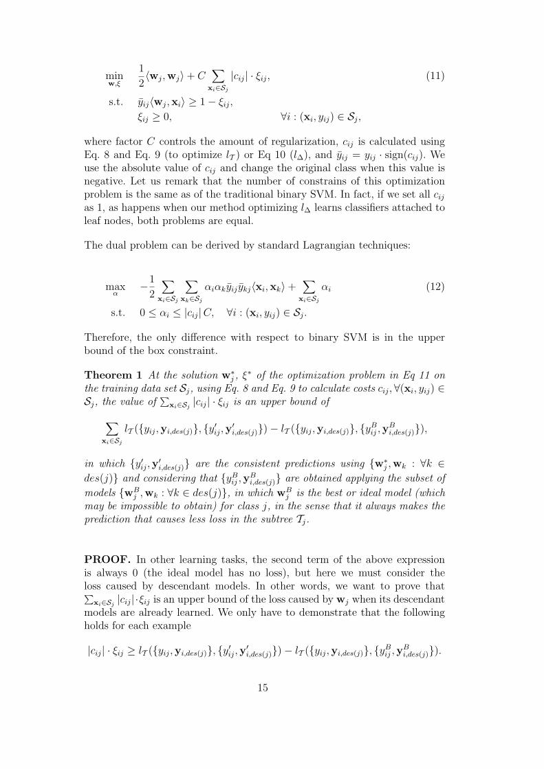
minw,ξ

1

2〈wj,wj〉+ C

∑xi∈Sj

|cij| · ξij, (11)

s.t. yij〈wj,xi〉 ≥ 1− ξij,ξij ≥ 0, ∀i : (xi, yij) ∈ Sj,

where factor C controls the amount of regularization, cij is calculated usingEq. 8 and Eq. 9 (to optimize lT ) or Eq 10 (l∆), and yij = yij · sign(cij). Weuse the absolute value of cij and change the original class when this value isnegative. Let us remark that the number of constrains of this optimizationproblem is the same as of the traditional binary SVM. In fact, if we set all cijas 1, as happens when our method optimizing l∆ learns classifiers attached toleaf nodes, both problems are equal.

The dual problem can be derived by standard Lagrangian techniques:

maxα

−1

2

∑xi∈Sj

∑xk∈Sj

αiαkyij ykj〈xi,xk〉+∑

xi∈Sj

αi (12)

s.t. 0 ≤ αi ≤ |cij|C, ∀i : (xi, yij) ∈ Sj.

Therefore, the only difference with respect to binary SVM is in the upperbound of the box constraint.

Theorem 1 At the solution w∗j , ξ∗ of the optimization problem in Eq 11 on

the training data set Sj, using Eq. 8 and Eq. 9 to calculate costs cij, ∀(xi, yij) ∈Sj, the value of

∑xi∈Sj

|cij| · ξij is an upper bound of

∑xi∈Sj

lT ({yij,yi,des(j)}, {y′ij,y′i,des(j)})− lT ({yij,yi,des(j)}, {yBij ,yBi,des(j)}),

in which {y′ij,y′i,des(j)} are the consistent predictions using {w∗j ,wk : ∀k ∈des(j)} and considering that {yBij ,yBi,des(j)} are obtained applying the subset of

models {wBj ,wk : ∀k ∈ des(j)}, in which wB

j is the best or ideal model (whichmay be impossible to obtain) for class j, in the sense that it always makes theprediction that causes less loss in the subtree Tj.

PROOF. In other learning tasks, the second term of the above expressionis always 0 (the ideal model has no loss), but here we must consider theloss caused by descendant models. In other words, we want to prove that∑

xi∈Sj|cij|·ξij is an upper bound of the loss caused by wj when its descendant

models are already learned. We only have to demonstrate that the followingholds for each example

|cij| · ξij ≥ lT ({yij,yi,des(j)}, {y′ij,y′i,des(j)})− lT ({yij,yi,des(j)}, {yBij ,yBi,des(j)}).

15

Following the definition in Eq 7, for negative examples we have that:

lT ({yij,yi,des(j)}, {yBij ,yBi,des(j)}) = min(0, fp(j) +∑

k∈y′i,des(j)

fp(k)) = 0.

Using Eq 8,

∣∣∣∣∣∣∣fp(j) +∑

k∈y′i,des(j)

fp(k)

∣∣∣∣∣∣∣ · ξij ≥ lT ({yij,yi,des(j)}, {y′ij,y′i,des(j)})− 0,

and this expression is always true because

lT ({yij,yi,des(j)}, {y′ij,y′i,des(j)})=

0 if 0 ≤ ξij < 1

fp(j)+∑k∈y′

i,des(j)fp(k) if ξij ≥ 1.

In the case of positive examples, lT ({yij,yi,des(j)}, {yBij ,yBi,des(j)}) is (using onceagain Eq 7)

min

∑k∈yi,des(j)−y′

i,des(j)

fn(k) +∑

k∈y′i,des(j)

−yi,des(j)

fp(k), fn(j) +∑

k∈yi,des(j)

fn(k)

. (13)

If the minimum is the first term (cij > 0 and yij = yij · sign(cij) = +1, seeEq 9), and now applying Eq 9,

∣∣∣∣∣∣∣fn(j) +∑

k∈yi,des(j)

fn(k)−∑

k∈yi,des(j)−y′i,des(j)

fn(k)−∑

k∈y′i,des(j)

−yi,des(j)

fp(k)

∣∣∣∣∣∣∣ · ξij ≥lT ({yij,yi,des(j)}, {y′ij,y′i,des(j)})−

∑k∈yi,des(j)−y′

i,des(j)

fn(k) +∑

k∈y′i,des(j)

−yi,des(j)

fp(k)

,and this is always true, because lT ({yij,yi,des(j)}, {y′ij,y′i,des(j)}) (see Eq 7) is

∑k∈yi,des(j)−y′

i,des(j)fn(k) +

∑k∈y′

i,des(j)−yi,des(j)

fp(k) if 0 ≤ ξij < 1

fn(j) +∑k∈yi,des(j)

fn(k) if ξij ≥ 1.

If the minimum in Eq 13 is the second term (cij < 0, yij = −1), then we have

16

to prove that

∣∣∣∣∣∣∣fn(j) +∑

k∈yi,des(j)

fn(k)−∑

k∈yi,des(j)−y′i,des(j)

fn(k)−∑

k∈y′i,des(j)

−yi,des(j)

fp(k)

∣∣∣∣∣∣∣ · ξij ≥lT ({yij,yi,des(j)}, {y′ij,y′i,des(j)})−

fn(j) +∑

k∈yi,des(j)

fn(k)

.And this inequality holds because lT ({yij,yi,des(j)}, {y′ij,y′i,des(j)}) is the oppo-site to that of the previous case (its original class is inverted in the optimizationproblem in Eq 11),

fn(j) +

∑k∈yi,des(j)

fn(k) if 0 ≤ ξij < 1∑k∈yi,des(j)−y′

i,des(j)fn(k) +

∑k∈y′

i,des(j)−yi,des(j)

fp(k) if ξij ≥ 1.

The case when both terms are equal (cij = 0) is trivial because

lT ({yij,yi,des(j)}, {y′ij,y′i,des(j)}) = lT ({yij,yi,des(j)}, {yBij ,yBi,des(j)}).

In fact, as mentioned previously, these examples are deleted from Sj. 2

The same demonstration can be employed to prove that, using Eq 10 to com-pute cij in the optimization problem equation (11), term

∑xi∈Sj

|cij| · ξij is anupper bound of the l∆ loss caused by w∗j , since l∆ is a particular case of thelT loss function.

4 Experimental results

The main aim of this section is to show that the method presented here canimprove the performance of the two decomposition algorithms, flat SVM andH-SVM , that are usually selected as baseline methods in papers that presentnew hierarchical classifiers. For that reason, we implemented, not only ourproposed algorithm H-SVMlT , but also another version of our approach, calledSVMlT , that is the counterpart method of flat SVM. Since we did not haveavailable functions fp and fn for the data sets used, both versions optimizedlocally (at every subtree) the loss function l∆ (Eq. 3). In the following wedenoted them as H-SVMl∆ and SVMl∆ , and the difference between them isthe same that between H-SVM and flat SVM: the data sets used to learn eachindividual binary classifier (see Eq. 4 and Eq. 5).

17

Let us recall that H-SVMl∆ and H-SVM use the same examples to learn eachmodel (applying Eq. 5 in step 4 of Algorithm 1). The only difference betweenthem is that the former optimizes locally (at every subtree) the hierarchi-cal loss function l∆ and H-SVM optimizes the binary zero-one loss function.The same occurs between, SVMl∆ and flat SVM, both use the same trainingpoints (all examples in this case, Eq. 4) and the difference, again, is that ourapproach learns cost-sensitive classifiers. Thus, since we are using l∆ as our tar-get loss function, classifiers at leaf nodes are exactly the same in H-SVMl∆ andH-SVM ; then, they only differ in those classifiers attached to internal nodes.The same happens between SVMl∆ and flat SVM.

Additionally, we wanted to compare our approach with two state-of-the-artlearners that use different methods. The algorithms used were H-M3 of Rousuet al. [6] and HMSVM of Lujuan et al. [5], both of them search for a globaloptimum loss (in this case the loss function l∆).

The comparison was done with three benchmark information retrieval (IR)data sets. Thus, in addition to our objective loss function l∆ (Eq. 3) and l0/1(Eq. 1), we also report the most common performance measures of IR tasks:precision, recall, and F1.

The implementation of H-M3 and HMSVM were provided by the authors whilethe implementation of the baseline algorithms (SVM and H-SVM ) and the ver-sions in which binary classifiers are not independent (SVMl∆ and H-SVMl∆ )were done modifying slightly Joachims’ SVMperf [20]; this SVM implemen-tation provided us with an excellent base due to its linear complexity. In allcases, when it was needed, we set the regularization parameter C = 1 andwe used a linear kernel. All the scores reported were estimated by means of astratified fivefold cross validation repeated two times. Following Demsar [21],we used the Wilcoxon signed-ranks test to compare the performance of twoclassifiers.

We used three well-known data sets in information retrieval 2 . The documentswere represented as bag-of-words and no word stemming or stop-word removalwas performed. The first data set, REUTERS Corpus Volume 1 (RCV1) [22],is composed of 7500 documents described by 19770 features. The ’CCAT’family of categories (Corporate/Industrial news articles) was used as the labelhierarchy. This hierarchy represents a tree with maximum depth 3 and with atotal of 34 nodes. The tree is quite unbalanced: there are 18 nodes residing indepth 1, 14 nodes in depth 2 and one node in depth 3 (see Figure 2a). In thisdata set, 8% of examples have multiple partial paths; that is, these examplesare classified into classes that are not in the same path from the root. The

2 These data sets can be downloaded from the following urls:http://users.ecs.soton.ac.uk/cjs/resource files/hierarchy data.tar.gzhttp://people.csail.mit.edu/jrennie/20Newsgroups/

18

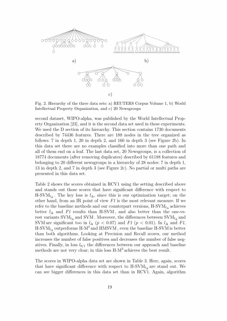
a) b)

c)

Fig. 2. Hierarchy of the three data sets: a) REUTERS Corpus Volume 1, b) WorldIntellectual Property Organization, and c) 20 Newsgroups

second dataset, WIPO-alpha, was published by the World Intellectual Prop-erty Organization [23], and it is the second data set used in these experiments.We used the D section of its hierarchy. This section contains 1730 documentsdescribed by 74436 features. There are 188 nodes in the tree organized asfollows: 7 in depth 1, 20 in depth 2, and 160 in depth 3 (see Figure 2b). Inthis data set there are no examples classified into more than one path andall of them end on a leaf. The last data set, 20 Newsgroups, is a collection of18774 documents (after removing duplicates) described by 61188 features andbelonging to 20 different newsgroups in a hierarchy of 28 nodes: 7 in depth 1,13 in depth 2, and 7 in depth 3 (see Figure 2c). No partial or multi paths arepresented in this data set.

Table 2 shows the scores obtained in RCV1 using the setting described aboveand stands out those scores that have significant difference with respect toH-SVMl∆ . The key loss is l∆, since this is our optimization target; on theother hand, from an IR point of view F1 is the most relevant measure. If werefer to the baseline methods and our counterpart versions, H-SVMl∆ achievesbetter l∆ and F1 results than H-SVM , and also better than the one-vs-rest variants SVMl∆ and SVM . Moreover, the differences between SVMl∆ andSVM are significant too in l∆ (p < 0.07) and F1 (p < 0.01). In l∆ and F1,H-SVMl∆ outperforms H-M3 and HMSVM , even the baseline H-SVM is betterthan both algorithms. Looking at Precision and Recall scores, our methodincreases the number of false positives and decreases the number of false neg-atives. Finally, in loss l0/1 the differences between our approach and baselinemethods are not very clear; in this loss H-M3 achieves the best result.

The scores in WIPO-alpha data set are shown in Table 3. Here, again, scoresthat have significant difference with respect to H-SVMl∆ are stand out. Wecan see bigger differences in this data set than in RCV1. Again, algorithm

19

Table 2Prediction losses l0/1, l∆, precision P, recall R and F1 (and standard deviations)on RCV1 data set. All scores are given as percentages, but the values of the columnlabeled by l∆ are the average of Eq. 3 across the test set. The best result in eachmeasure is highlighted in bold. When the difference between H-SVMl∆ and anotheralgorithm is statistically significant in a Wilcoxon signed-ranks test with thresholdof 0.05 then a † or a ∗ is attached to the value. The † indicates that the corre-sponding algorithm is significantly better than H-SVMl∆ , whereas a ∗ indicatesthat H-SVMl∆ is significantly better than the other algorithm

l0/1 l∆ P R F1

SVM 27.18∗±1.09 0.504∗±0.027 93.31†±0.81 68.94∗±1.56 79.29∗±1.17

SVMl∆ 27.61∗±0.93 0.500∗±0.024 92.64†±0.60 69.83∗±1.36 79.63∗±1.02

H-SVM 24.20 ±0.99 0.475 ±0.027 90.56†±0.89 73.77∗±1.42 81.30∗±1.08

H-SVMl∆ 24.38 ±0.91 0.473±0.027 89.31 ±1.02 75.16 ±1.54 81.62 ±1.07

H-M3 23.39†±1.15 0.490∗±0.032 89.51 ±0.90 73.59∗±1.72 80.77∗±1.29

HMSVM 28.44∗±1.02 0.743∗±0.033 93.21†±0.86 50.60∗±1.97 65.58∗±1.76

Table 3Prediction losses l0/1, l∆, precision P, recall R and F1 (and standard deviations)on WIPO-alpha data set. See column and symbol descriptions in Table 2

l0/1 l∆ P R F1

SVM 83.60∗±2.34 1.641∗±0.029 94.99†±1.11 62.27∗±0.53 75.22∗±0.39

SVMl∆ 82.34∗±4.01 1.621∗±0.043 94.20†±1.22 63.41∗±1.28 75.78∗±0.79

H-SVM 74.44∗±3.31 1.553∗±0.055 92.77†±1.22 66.38∗±1.97 77.36∗±1.11

H-SVMl∆ 71.58 ±2.12 1.512±0.060 90.76 ±1.12 69.27 ±1.03 78.57 ±0.88

H-M3 69.33†±1.94 1.582∗±0.061 91.92†±1.23 66.29∗±1.40 77.02∗±1.00

HMSVM 53.83†±2.42 2.240∗±0.139 72.00∗±1.74 72.00†±1.74 72.00∗±1.74

H-SVMl∆ outperforms the rest of algorithms in l∆ and F1. Differences betweenSVM and SVMl∆ are significant too in l∆ (p < 0.02) and F1 (p < 0.01). In thisdata set, HMSVM obtains the best result in the loss l0/1 and there is a bigdifference between H-SVMl∆ and its counterpart H-SVM , although in the one-vs-rest variants the difference is smaller.

The same behavior is presented in the scores of 20 Newsgroups dataset (Ta-ble 4). Here again, H-SVMl∆ achieves better l∆ and F1 results than H-SVM ,and also better than the one-vs-rest variants SVMl∆ and SVM . Differencesbetween SVMl∆ and SVM are significant too in l∆ and F1 (p < 0.01). In thisdata set, best results are achieved by HMSVM .

We can appreciate that the proposed algorithms perform better in the WIPO-alpha data set. The reason of that behavior is that, paying attention to the

20

Table 4Prediction losses l0/1, l∆, precision P, recall R and F1 (and standard deviations)on 20 Newsgroups data set. See column and symbol descriptions in Table 2

l0/1 l∆ P R F1

SVM 35.64∗±1.16 0.716∗±0.029 89.92∗±0.48 87.44†±0.65 88.66∗±0.47

SVMl∆ 35.59∗±1.22 0.714∗±0.030 89.93∗±0.55 87.51†±0.57 88.70 ±0.46

H-SVM 30.82 ±1.16 0.696∗±0.030 92.02 ±0.41 85.71∗±0.67 88.75∗±0.51

H-SVMl∆ 30.78 ±1.17 0.694 ±0.030 92.01 ±0.46 85.78 ±0.65 88.79 ±0.50

H-M3 34.98∗±1.64 0.687 ±0.037 93.11†±1.12 84.85∗±0.90 88.78 ±0.59

HMSVM 18.06†±0.69 0.582†±0.025 90.92∗±0.38 90.89†±0.41 90.91†±0.40

hierarchies in Figure 2, RCV1 and 20 Newsgroups data sets have a more simplehierarchy, with several nodes at depth 1. In fact, in RCV1, H-SVMl∆ andH-SVM only differ in seven out of 34 binary classifiers (the number of internalnodes), and only four of them have a hierarchy with more than two nodes. Asimilar situation is presented in 20 Newsgroup data set where they only differin seven out of 28 binary classifiers. The hierarchy of WIPO-alpha is biggerand there are many nodes at different levels. In this case, there are many moreinternal nodes and most of them have several descendants. This suggests thatour method can improve more the performance of H-SVM in those data setsin which the hierarchical structure is more complex.

In our opinion, these results show that we need to consider the existent depen-dencies between individual classifiers in order to build a useful decompositionhierarchical learning algorithm based on binary SVMs. Our method exploitsthis aspect, capturing some of those dependencies, thanks to every individualmodel is learned considering its descendant classifiers and optimizing locallya function loss appropriated to hierarchical classification tasks.

5 Conclusions

In this paper, we have presented a learning method for hierarchical classifi-cations tasks based on the decomposition approach: our learner is composedof a set of individual binary cost-sensitive classifiers, one for each class of thehierarchy. The main novelty of our approach is that these models are not in-dependent from one another, as usually occurs in decomposition approaches.Each individual classifier depends on the models of its descendant classes. Thealgorithm is based on the use of a bottom-up learning procedure that allowsa generic hierarchical loss function to be considered when models are learned.In the experiments reported in Section 4, we also confirm the good scores of

21

this approach against both, state-of-the-art algorithms like [5,6] and baselinemethods.

One of the aims of this work is to prove that decomposition methods canbe as useful in hierarchical classification tasks as in multiclass classificationwhere this kind of approach is widely used in real applications. Additionally,decomposition strategies generally have the advantage of modularity. It is thuspossible to have fast parallel implementations for hierarchical classifications.Moreover, each binary classification could be learned using well-known SVMimplementations, and the regularization parameters or the kernels employedmay be tuned. As always, the choice of the right kernel may be a crucial pointin the performance of any classification task.

Acknowledgements

The authors would like to thank Juho Rousu, Thorsten Joachims and LijuanCai for the source code of H-M3 , SVMPerf and HMSVM , respectively.

The research reported in this paper has been supported in part under SpanishMinisterio de Ciencia e Innovacion (MICINN) Grant TIN2008-06247 and bythe Fundacion para la Investigacion Cientıfica y Tecnica (FICYT), Asturias,Spain, under Grant IB09-059-C2.

References

[1] D. Koller and M. Sahami, “Hierarchically classifying documents using very fewwords,” in ICML’97: Proceedings of the International Conference on MachineLearning, pp. 170–178, 1997.

[2] S. T. Dumais and H. Chen, “Hierarchical classification of web content,” inSIGIR-00: Proceedings of the on Research and Development in InformationRetrieval, (New York, NY, USA), pp. 256–263, ACM Press, 2000.

[3] N. Cesa-Bianchi, C. Gentile, and L. Zaniboni, “Incremental algorithms forhierarchical classification,” Journal of Machine Learning Research, vol. 7,pp. 31–54, 2006.

[4] L. Cai and T. Hofmann, “Hierarchical document categorization with supportvector machines,” in CIKM ’04: Proceedings of the 13th ACM InternationalConference on Information and Knowledge Management, (New York, NY,USA), pp. 78–87, ACM Press, 2004.

22

[5] L. Cai and T. Hofmann, “Exploiting known taxonomies in learning overlappingconcepts,” in IJCAI ’07: Proceedings of the 20th International Joint Conferenceon Artificial Intelligence, pp. 708–713, 2007.

[6] J. Rousu, C. Saunders, S. Szedmak, and J. Shawe-Taylor, “Kernel-basedlearning of hierarchical multilabel classification models,” Journal of MachineLearning Research, vol. 7, pp. 1601–1626, 2006.

[7] O. Dekel, J. Keshet, and Y. Singer, “Large margin hierarchical classification,” inProceedings of the 21st International Conference on Machine learning, pp. 209–216, 2004.

[8] O. Dekel, J. Keshet, and Y. Singer, “An efficient online algorithm forhierarchical phoneme classification,” in Proceedings of 1st InternationalWorkshop on Machine Learning for Multimodal Interaction, pp. 146–158, 2005.

[9] J. Sinapov and A. Stoytchev, “Detecting the functional similarities betweentools using a hierarchical representation of outcomes,” in 7th IEEEInternational Conference on Development and Learning, 2008. ICDL 2008,pp. 91–96, 2008.

[10] M. Ashburner, C. Ball, J. Blake, D. Botstein, H. Butler, J. Cherry, A. Davis,K. Dolinski, S. Dwight, J. Eppig, et al., “Gene Ontology: tool for the unificationof biology,” Nature genetics, vol. 25, no. 1, pp. 25–29, 2000.

[11] Z. Barutcuoglu, R. Schapire, and O. Troyanskaya, “Hierarchical multi-labelprediction of gene function,” Bioinformatics, vol. 22, no. 7, pp. 830–836, 2006.

[12] J. Bo, M. Brian, Z. Chengxiang, and L. Xinghua, “Multi-label literatureclassification based on the Gene Ontology graph,” BMC Bioinformatics, vol. 9,2008.

[13] G. Tsoumakas and I. Katakis, “Multi-Label Classification: An Overview,”International Journal of Data Warehousing and Mining, vol. 3, no. 3, pp. 1–13,2007.

[14] M.-L. Zhang and Z.-H. Zhou, “Ml-knn: A lazy learning approach to multi-labellearning,” Pattern Recognition, vol. 40, no. 7, pp. 2038 – 2048, 2007.

[15] R. Schapire and Y. Singer, “BoosTexter: A boosting-based system for textcategorization,” Machine learning, vol. 39, no. 2, pp. 135–168, 2000.

[16] C. Vens, J. Struyf, L. Schietgat, S. Dzeroski, and H. Blockeel, “Decision treesfor hierarchical multi-label classification,” Machine Learning, vol. 73, no. 2,pp. 185–214, 2008.

[17] C.-W. Hsu and C.-J. Lin, “A comparison of methods for multiclass supportvector machines,” Neural Networks, IEEE Transactions on, vol. 13, no. 2,pp. 415–425, 2002.

[18] C. Elkan, “The foundations of cost-sensitive learning,” in In Proceedings of theSeventeenth International Joint Conference on Artificial Intelligence, pp. 973–978, 2001.

23

[19] H. Fan and K. Ramamohanarao, “A weighting scheme based on emergingpatterns for weighted support vector machines,” in Proceedings of IEEEInternational Conference on Granular Computing, pp. 435– 440, 2005.

[20] T. Joachims, “Training linear svms in linear time,” in KDD ’06: Proceedings ofthe 12th ACM SIGKDD International Conference on Knowledge Discovery andData Mining, (New York, NY, USA), pp. 217–226, ACM Press, 2006.

[21] J. Demsar, “Statistical Comparisons of Classifiers over Multiple Data Sets,”Journal of Machine Learning Research, vol. 7, pp. 1–30, 2006.

[22] D. D. Lewis, Y. Yang, T. G. Rose, and F. Li, “Rcv1: A new benchmark collectionfor text categorization research,” The Journal of Machine Learning Research,vol. 5, pp. 361–397, 2004.

[23] WIPO, “World intellectual property organization,”http://www.wipo.int/classifications/en, 2001.

24