Research Article A Seed-Based Plant Propagation Algorithm: The Feeding Station Model Muhammad Sulaiman 1,2 and Abdellah Salhi 1 1 Department of Mathematical Sciences, University of Essex, Colchester CO4 3SQ, UK 2 Department of Mathematics, Abdul Wali Khan University, Mardan, Khyber Pakhtunkhwa, Pakistan Correspondence should be addressed to Muhammad Sulaiman; [email protected] Received 25 December 2014; Revised 10 February 2015; Accepted 10 February 2015 Academic Editor: Xinyu Li Copyright © 2015 M. Sulaiman and A. Salhi. is is an open access article distributed under the Creative Commons Attribution License, which permits unrestricted use, distribution, and reproduction in any medium, provided the original work is properly cited. e seasonal production of fruit and seeds is akin to opening a feeding station, such as a restaurant. Agents coming to feed on the fruit are like customers attending the restaurant; they arrive at a certain rate and get served at a certain rate following some appropriate processes. e same applies to birds and animals visiting and feeding on ripe fruit produced by plants such as the strawberry plant. is phenomenon underpins the seed dispersion of the plants. Modelling it as a queuing process results in a seed- based search/optimisation algorithm. is variant of the Plant Propagation Algorithm is described, analysed, tested on nontrivial problems, and compared with well established algorithms. e results are included. 1. Introduction Plants have evolved a variety of ways to propagate. Propaga- tion with seeds is perhaps the most common of them all and one which takes advantage of all sorts of agents ranging from wind to water, birds, and animals. In [1] a Plant Propagation Algorithm based on the way the strawberry plant propagates using runners has been introduced. Here, we consider the case where the strawberry plant uses seeds to propagate. Plants rely heavily on the dispersion of their seeds to colonise new territories and to improve their survival [2, 3]. ere are a lot of studies and models of seed dispersion particularly for trees [2–6]. Dispersion by wind and ballistic means is probably the most studied of all approaches [7– 9]. However, in the case of the strawberry plant, given the way the seeds stick to the surface of the fruit (Figure 1(a)) [10], dispersion by wind or mechanical means is very limited. Animals, however, and birds in particular are the ideal agents for dispersion [2, 3, 11, 12] in this case. ere are many biologically inspired optimization algo- rithms in the literature [13, 14]. e Flower Pollination Algorithm (FPA) is inspired by the pollination of flowers through different agents [8]; the swarm data clustering algo- rithm is inspired by pollination by bees [15]; Particle Swarm Optimization (PSO) is inspired by the foraging behavior of groups of animals and insects [16, 17]; the Artificial Bee Colony (ABC) simulates the foraging behavior of honey bees [18, 19]; the Firefly algorithm is inspired by the flashing fireflies when trying to attract a mate [20, 21]; the Social Spider Optimization (SSO) algorithm is inspired by the cooperative behavior of social spiders [22]. e list could easily be extended. e Plant Propagation Algorithm (PPA) also known as the strawberry algorithm was inspired by the way plants and specifically the strawberry plants propagate using runners [1, 23]. e attraction of PPA is that it can be implemented easily for all sorts of optimization problems. Moreover, it has few algorithm specific arbitrary parameters. It follows the principle that plants in good spots with plenty of nutrients will send many short runners. ey send few long runners when in nutrient poor spots. With long runners PPA tries to explore the search space while short runners enable it to exploit the solution space well. In this paper, we investigate an alternative PPA which is entirely based on the propagation by seeds of the strawberry plant. Because of the periodic nature of fruit and seed production, it amounts to setting up a feeding station for the attention of potential seed-dispersing agents [24], Hence the feeding station model used here and the resulting Seed-Based Plant Propagation Algorithm or SbPPA. Hindawi Publishing Corporation e Scientific World Journal Volume 2015, Article ID 904364, 16 pages http://dx.doi.org/10.1155/2015/904364

Welcome message from author
This document is posted to help you gain knowledge. Please leave a comment to let me know what you think about it! Share it to your friends and learn new things together.
Transcript
Research ArticleA Seed-Based Plant Propagation AlgorithmThe Feeding Station Model
Muhammad Sulaiman12 and Abdellah Salhi1
1Department of Mathematical Sciences University of Essex Colchester CO4 3SQ UK2Department of Mathematics Abdul Wali Khan University Mardan Khyber Pakhtunkhwa Pakistan
Correspondence should be addressed to Muhammad Sulaiman sulaiman513yahoocouk
Received 25 December 2014 Revised 10 February 2015 Accepted 10 February 2015
Academic Editor Xinyu Li
Copyright copy 2015 M Sulaiman and A Salhi This is an open access article distributed under the Creative Commons AttributionLicense which permits unrestricted use distribution and reproduction in any medium provided the original work is properlycited
The seasonal production of fruit and seeds is akin to opening a feeding station such as a restaurant Agents coming to feed onthe fruit are like customers attending the restaurant they arrive at a certain rate and get served at a certain rate following someappropriate processes The same applies to birds and animals visiting and feeding on ripe fruit produced by plants such as thestrawberry plantThis phenomenon underpins the seed dispersion of the plants Modelling it as a queuing process results in a seed-based searchoptimisation algorithm This variant of the Plant Propagation Algorithm is described analysed tested on nontrivialproblems and compared with well established algorithms The results are included
1 Introduction
Plants have evolved a variety of ways to propagate Propaga-tion with seeds is perhaps the most common of them all andone which takes advantage of all sorts of agents ranging fromwind to water birds and animals In [1] a Plant PropagationAlgorithm based on the way the strawberry plant propagatesusing runners has been introduced Here we consider thecase where the strawberry plant uses seeds to propagate
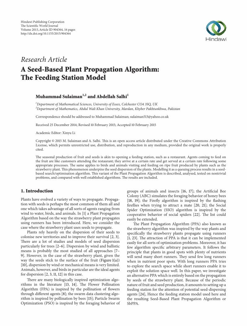
Plants rely heavily on the dispersion of their seeds tocolonise new territories and to improve their survival [2 3]There are a lot of studies and models of seed dispersionparticularly for trees [2ndash6] Dispersion by wind and ballisticmeans is probably the most studied of all approaches [7ndash9] However in the case of the strawberry plant given theway the seeds stick to the surface of the fruit (Figure 1(a))[10] dispersion by wind or mechanical means is very limitedAnimals however and birds in particular are the ideal agentsfor dispersion [2 3 11 12] in this case
There are many biologically inspired optimization algo-rithms in the literature [13 14] The Flower PollinationAlgorithm (FPA) is inspired by the pollination of flowersthrough different agents [8] the swarm data clustering algo-rithm is inspired by pollination by bees [15] Particle SwarmOptimization (PSO) is inspired by the foraging behavior of
groups of animals and insects [16 17] the Artificial BeeColony (ABC) simulates the foraging behavior of honey bees[18 19] the Firefly algorithm is inspired by the flashingfireflies when trying to attract a mate [20 21] the SocialSpider Optimization (SSO) algorithm is inspired by thecooperative behavior of social spiders [22] The list couldeasily be extended
The Plant Propagation Algorithm (PPA) also known asthe strawberry algorithm was inspired by the way plants andspecifically the strawberry plants propagate using runners[1 23] The attraction of PPA is that it can be implementedeasily for all sorts of optimization problems Moreover it hasfew algorithm specific arbitrary parameters It follows theprinciple that plants in good spots with plenty of nutrientswill send many short runners They send few long runnerswhen in nutrient poor spots With long runners PPA triesto explore the search space while short runners enable it toexploit the solution space well In this paper we investigatean alternative PPAwhich is entirely based on the propagationby seeds of the strawberry plant Because of the periodicnature of fruit and seed production it amounts to setting up afeeding station for the attention of potential seed-dispersingagents [24] Hence the feeding station model used here andthe resulting Seed-Based Plant Propagation Algorithm orSbPPA
Hindawi Publishing Corporatione Scientific World JournalVolume 2015 Article ID 904364 16 pageshttpdxdoiorg1011552015904364
2 The Scientific World Journal
(a) Strawberry fruit with seeds (b) Strawberry flower (c) A strawberry eaten by bird(s)
(d) A bird eating strawberries (e) Strawberry plants showing runners and seededfruit
Figure 1 Strawberry plant propagation through seed dispersion [25ndash28]
SbPPA is tested on both unconstrained and constrainedbenchmark problems also used in [22 29 30] Experimentalresults are presented in Tables 4ndash7 in terms of best meanworst and standard deviation for all algorithms The paperis organised as follows In Section 2 we briefly introducethe feeding station model representing strawberry plants infruit and the main characteristics of the paths followed bydifferent agents that disperse the seeds Section 3 presentsthe SbPPA in pseudocode form The experimental settingsresults and convergence graphs for different problems aregiven in Section 4
2 Aspects of the Feeding Station Model
Some animals and plants depend on each other to conservetheir species [31]Thusmany plants require for effective seed
dispersal the visits of frugivorous birds or animals accordingto a certain distribution [2 3 32 33]
Seed dispersal by different agents is also called ldquoseedshadowrdquo [32] this shows the abundance of seeds spreadglobally or locally around parent plants Here a queuingmodel is used which in the context of a strawberry feedingstation model involves two parts
(1) the quantity of fruit or seeds available to agents whichimplies the rate at which the agents will visit theplants
(2) a probability density function that tells us about theservice rate with which the agents are served by theplants
The model estimates the quantity of seeds that is spreadlocally compared to that dispersed globally [34ndash38] Thereare two aspects that need to be balanced exploitation which
The Scientific World Journal 3
is represented by the dispersal of seeds around the plantsand exploration which ensures that the search space is wellcovered
Agents arrive at plants in a random process Assumethat at most one agent arrives to the plants in any unit oftime (orderliness condition) It is further supposed that theprobability of arrivals of agents to the plants remains thesame for a particular period of timeThis period correspondsto when the plants are in fruit and during which timethe number of visitors is stable (stationarity condition)Furthermore it is assumed that the arrival of one agent doesnot affect the rest of arrivals (independence)
With these assumptions in mind the arrival of agentsto plants follows a Poisson process [39 40] which can beformally described as follows Let 1198831015840 be the random variablerepresenting the number of arrivals per unit of time 119905 Thenthe probability of 119896 arrivals over 119905 is
119875 (1198831015840= 119896) =
(120582119905)119896119890minus120582119905
119896 (1)
where 120582 denotes the mean arrival rate of agents per time unit119905 On the other hand the time taken by agents in successfullyeating fruit and leaving to disperse its seeds in other wordsthe service time for agents is expressed by a random variablewhich follows the exponential probability distribution [41]This can be expressed as follows
119878 (119905) = 120583119890minus120583119905 (2)
where 120583 is the average number of agents that can feed at time119905 Let us assume that the arrival rate of agents is less than thefruits available on all plants per unit of time therefore 120582 lt 120583
We assume that the system is in steady state Let119860 denotethe average number of agents in the strawberry field (somealready eating and the rest waiting to feed) and119860
119902the average
number of agents waiting to get the chance to feed If wedenote the average number of agents eating fruits by120582120583 thenby Littlersquos formula [42] we have
119860 = 119860119902+120582
120583 (3)
Since the plant needs to maximise dispersion this isequivalent to having a large 119860
119902in (3) Therefore from this
equation we need to solve the following problem
Maximize 119860119902= 119860 minus
120582
120583
subject to 1198921(120582 120583) = 120582 lt 120583 + 1
120582 gt 0 120583 gt 0
(4)
where 119860 = 10 which represents the population size in theimplementationThe simple limits on the variables are 0 lt 120582120583 le 100 The optimum solution to this particular problem is120582 = 11 120583 = 01 and 119860
119902= 1
Frugivores may travel far away from the plants and hencewill disperse the seeds far and wide This feeding behaviourtypically follows a Levy distribution [43ndash45] In the followingwe present some basic facts about it
21 Levy Distribution The Levy distribution is a probabilitydensity distribution for random variables Here the randomvariables represent the directions of flights of arbitrary birdsThis function ranges over real numbers in the domainrepresented by the problem search space
The flight lengths of the agents served by the plants followa heavy tailed power law distribution [14] represented by
119871 (119904) sim |119904|minus1minus120573
(5)
where 119871(119904) denotes the Levy distribution with index 120573 isin
(0 2) Levy flights are unique arbitrary excursions whose steplengths are drawn from (5) An alternative form of Levydistribution is [14]
119871 (119904 120574 120583) =
radic120574
2120587(
1
(119904 minus 120583))
32
sdot exp[minus120574
2 (119904 minus 120583)] 0 lt 120583 lt 119904 lt infin
0 Otherwise
(6)
This implies that
lim119904rarrinfin
119871 (119904 120574 120583) asymp radic120574
2120587(1
119904)
32
(7)
In terms of the Fourier transform [14] the limiting value of119871(119904) can be written as
lim119904rarrinfin
119871 (119904) =120572120573Γ (120573) sin (1205871205732)
120587 |119904|1+120573
(8)
where Γ(120573) is the Gamma function [46] defined by
Γ (120573) = int
infin
0
119909120573minus1
119890minus119909119889119909 (9)
The steps 119871(119904) are generated by Mantegnarsquos algorithm [14]This algorithm ensures that the behaviour of Levy flights issymmetric and stable as shown in Figure 3(b)
3 Strawberry Plant Propagation AlgorithmThe Feeding Station Model
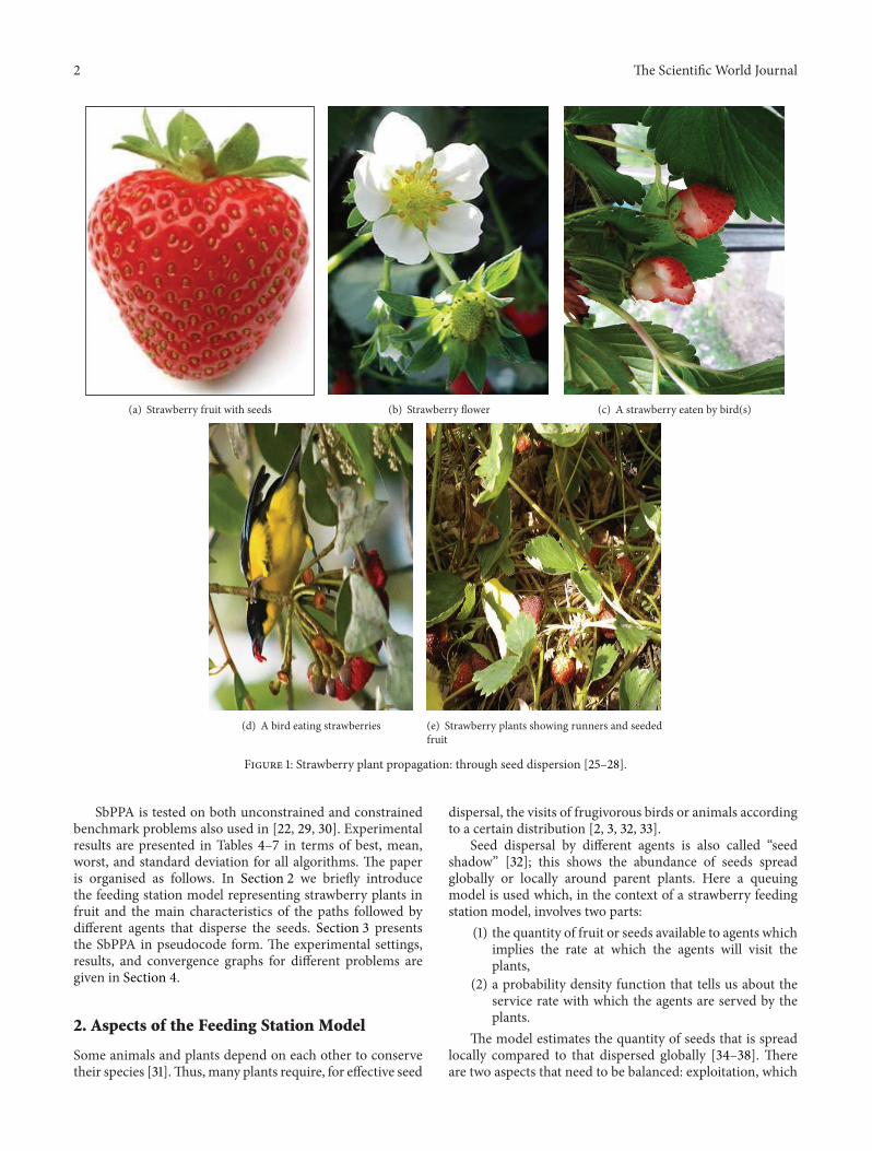
We assume that the arrival of different agents (birds andanimals) to the plants to feed is according to the Poissondistribution [40] As per the solution of problem (4) themean arrival rate is 120582 = 11 and NP = 10 is the size ofthe agents population Let 119896 = 1 2 119860 be the possiblenumbers of agents visiting the plants per unit time Withthese assumptions the graphic representation of (1) results inFigure 2
As already stated it is essential in this algorithm tobalance exploration and exploitation To this end we choosea threshold value of the Poisson probability that dictateshow much exploration and exploitation are done duringthe search The probability Poiss(120582) lt 005 means that
4 The Scientific World JournalPr
obab
ilitie
s Po
iss(120582)
Arrival rate of agents per unit time
025
02
015
01
005
00 2 4 6 8 10
Figure 2 Distribution of agents arriving at strawberry plants to eatfruit and disperse seeds
exploitation is covered In this case (10) below is used whichhelps the algorithm to search locally
119909lowast
119894119895=
119909119894119895+ 120585119895(119909119894119895minus 119909119897119895) if PR le 08 119895 = 1 2 119899
119894 119897 = 1 2 NP 119894 = 119897
119909119894119895 Otherwise
(10)
where PR denotes the rate of dispersion of the seeds locallyaround SP 119909lowast
119894119895and 119909
119894119895isin [119886119895119887119895] are the 119895th coordinates of
the seeds 119883lowast119894and119883
119894 respectively 119886
119895and 119887119895are the 119895th lower
and upper bounds defining the search space of the problemand 120585119895isin [minus1 1] The indices 119897 and 119894 are mutually exclusive
On the other hand if Poiss(120582) ge 005 then global disper-sion of seeds becomes more prominent This is implementedby using the following equation
119909lowast
119894119895=
119909119894119895+ 119871119894(119909119894119895minus 120579119895) if PR le 08 120579
119895isin [119886119895119887119895]
119894 = 1 2 NP
119895 = 1 2 119899
119909119894119895 Otherwise
(11)
where 119871119894is a step drawn from the Levy distribution [14] and
120579119895is a random coordinate within the search space Equations
(10) and (11) perturb the current solution the results of whichcan be seen in Figures 3(a) and 3(b) respectively
As mentioned in Algorithm 1 we first collect the bestsolutions from the first NP trial runs to form a populationof potentially good solutions denoted by popbest The conver-gence rate of SbPPA is shown in Figures 4 and 5 for differenttest problems used in our experiments (see Appendices) Thestatistics values best worst mean and standard deviation arecalculated based on popbest
The seed-based propagation process of SP can be repre-sented in the following steps
Sear
ch sp
ace
Spring Design Problem
times105
15
10
5
0
minus5
minus10
minus150 2 4 6
(a) Perturbations by (10)Se
arch
spac
eSpring Design Problem
times105
40
20
0
minus20
minus40
minus60
minus800 5 10 15
(b) Perturbations by (11)
Figure 3Overall performance of SbPPAonSpringDesignProblem
(1) The dispersal of seeds in the neighbourhood of theSP as shown in Figure 1(e) is carried out either byfruits fallen from strawberry plants after they becomeripe or by agents The step lengths for this phase arecalculated using (10)
(2) Seeds are spread globally through agents as shownin Figures 1(c) and 1(d) The step lengths for thesetravelling agents are drawn from the Levy distribution[14]
(3) The probabilities Poiss(120582) that a certain number 119896 ofagents will arrive to SP to eat fruits and disperse it
The Scientific World Journal 5
(1) NPlarr Population size 119903 larr Counter of trial runs MaxExp larrMaximum experiments(2) for 119903 = 1 MaxExp do(3) if 119903 le NP then(4) Create a random population of seeds pop = 119883
119894| 119894 = 1 2 NP
using (12) and collect the best solutions from each trial run in popbest(5) Evaluate the population pop(6) end if(7) while 119903 gt NP do(8) Use updated population popbest(9) end while(10) while (the stopping criteria is not satisfied) do(11) for 119894 = 1 to NP do(12) if Poiss(120582)
119894ge 005 then ⊳ (Global or local seed dispersion)
(13) for 119895 = 1 to 119899 do ⊳ (119899 is number of dimensions)(14) if rand le PR then ⊳ (PR = Perturbation Rate)(15) Update the current entry according to (11)(16) end if(17) end for(18) else(19) for 119895 = 1 to 119899 do(20) if rand le PR then(21) Update the current entry according to (10)(22) end if(23) end for(24) end if(25) end for(26) Update current best(27) end while(28) Return Updated population and global best solution(29) end for
Algorithm 1 Seed-based Plant Propagation Algorithm (SbPPA) [47]
is used as a balancing factor between exploration andexploitation
For implementation purposes we assume that each SPproduces one fruit and each fruit is assumed to have oneseed by a solution119883
119894wemean the current position of the 119894th
seed to be dispersed The number of seeds in the populationis denoted by NP Initially we generate a random populationof NP seeds using
119909119894119895= 119886119895+ (119887119895minus 119886119895) 120578119895 119895 = 1 119899 (12)
where 119909119894119895
isin [119886119895119887119895] is the 119895th coordinate of solution 119883
119894 119886119895
and 119887119895are the 119895th coordinates of the bounds describing the
search space of the problem and 120578119895isin (0 1) This means that
119883119894= [119909119894119895] for 119895 = 1 119899 represents the position of the 119895th
seed in population pop
4 Experimental Settings and Discussion
In our experiments we tested SbPPA against some recentlydeveloped algorithms and somewell established and standardones Our set of test problems includes benchmark con-strained and unconstrained optimization problems [22 3048 49] The results are compared in terms of statistics (bestworst mean and standard deviation) for solutions obtained
by SbPPA ABC [18 50] PSO [51] FF [21] HPA [29] SSO-C [22] Classical Evolutionary Programming (CEP) [30] andFast Evolutionary Programming (FEP) [30] The detaileddescriptions of these problems are given in Appendices
In Tables 4 and 7 the significance of results is shown interms of wintieloss (see Table 2 in [52]) according to thefollowing notations
(i) (+) when SbPPA is better(ii) (asymp) when the results are approximately the same as
those obtained with SbPPA(iii) (minus) when SbPPA is worse
Moreover in Tables 5 and 6 the significance of resultsobtained with SbPPA is highlighted
41 Parameter Settings The parameter settings are given inTables 1ndash3
5 Conclusion
In this paper a new metaheuristic referred to as the Seed-Based Plant Propagation Algorithm (SbPPA) [47] has beenproposed Plants have evolved a variety of ways to propagatePropagation through seeds is perhaps the most commonof them all and one which takes advantage of all sorts of
6 The Scientific World Journal
0 5 10 15 20 25 30
0020406
Total trial runs
Obj
ectiv
e val
ueConvergence plot of f1
(a)
5 10 15 20 25 3002468
Total trial runs
Obj
ectiv
e val
ue
times10minus9 Convergence plot of f2
(b)
0 5 10 15 20 25 30
01234
Total trial runs
Obj
ectiv
e val
ue
times10minus5 Convergence plot of f3
(c)
5 10 15 20 25 30minus50
minus49998minus49996minus49994minus49992
Total trial runs
Obj
ectiv
e val
ue
Convergence plot of f5
(d)
0 5 10 15 20 25 30minus210minus209minus208minus207
Total trial runs
Obj
ectiv
e val
ues
Convergence plot of f6
(e)
0 5 10 15 20 25 300123
Total trial runs
Obj
ectiv
e val
ues times10
minus4 Convergence plot of f10
(f)
Figure 4 Performance of SbPPA on unconstrained global optimization problems
Obj
ectiv
e val
ue
Total trail runs
Convergence plot of CP1
0 5 10 15 20 25 30
minus149999
minus15
minus15
minus15
minus15
(a)
Obj
ectiv
e val
ue
Total trail runs
Convergence plot of CP2
0 5 10 15 20 25 30
times104
minus30662
minus30663
minus30664
minus30665
minus30666
(b)
Obj
ectiv
e val
ue
Total trail runs
Convergence plot of CP3
0 5 10 15 20 25 30
minus6880
minus6900
minus6920
minus6940
minus6960
minus6980
(c)
Obj
ectiv
e val
ue
Total trail runs
Convergence plot of CP4
0 5 10 15 20 25 30
27
26
25
24
(d)
Obj
ectiv
e val
ue
Total trail runs
Convergence plot of CP5
0 5 10 15 20 25 30
085
08
075
07
(e)
Obj
ectiv
e val
ue
Total trail runs
Convergence plot of Spring Design Problem
0 5 10 15 20 25 30
2996125
299612
2996115
299611
(f)
Figure 5 Performance of SbPPA on constrained global optimization problems (see Appendices)
The Scientific World Journal 7
Table1Parametersu
sedfore
achalgorithm
forsolving
unconstrainedglob
alop
timizationprob
lems1198911ndash11989110A
llexperim
entsarer
epeated30
times
PSO[1629]
ABC
[1829]
HPA
[29]
SbPP
A[47]
119872=100
SN=100
Agents=
100
NP=10
119866max=(Dim
ensio
ntimes20000)
119872MCN
=(Dim
ensio
ntimes20000)
SNIte
ratio
nnu
mber=
(Dim
ensio
ntimes20000)
Agents
Iteratio
nnu
mber=
(Dim
ensio
ntimes20000)
NP
119888 1=2
MR=08
119888 1=2
PR=08
119888 2=2
Limit=(SN
timesdimensio
n)2
119888 2=2
Poiss(120582)=005
119882=(119866
maxminusiteratio
n ind
ex)
119866max
mdashLimit=(Agentstimes
dimensio
n)2
mdash
mdashmdash
119882=(Ite
ratio
nnu
mberminus
iteratio
n ind
ex)
Iteratio
nnu
mber
mdash
8 The Scientific World Journal
Table 2 Experimental setup used for each algorithm for solvingunconstrained global optimization problems 119891
11ndash11989126 All experi-
ments are repeated 50 times
CEP [30 53 54] FEP [30] SbPPAPopulation size120583 = 100
Population size120583 = 100
NP = 10
Tournament size119902 = 10
Tournament size119902 = 10 PR = 08
120578 = 30 120578 = 30 Poiss(120582) = 005
agents ranging from wind to water birds and animals Thestrawberry plant uses both runners and seeds to propagateHere we consider the propagation through seeds that thestrawberry plant has evolved to design an efficient optimiza-tion algorithm
To capture the dispersal process we adopt a queuingapproach which given the extent of fruit produced indicatesthe extent of seeds dispersed and hence the effectivenessof the searchoptimization algorithm based on this processLooking at the random process of agents using the plants(feeding station) it is reasonable to assume that it is of thePoisson type On the other hand the time taken by agentsin successfully eating fruit and leaving to disperse its seedsin other words the service time for agents is expressed by arandom variable which follows the exponential probabilitydistribution To this end we choose a threshold value ofthe Poisson probability that dictates how much explorationand exploitation are done during the search An alternativestrategy has been adopted here This strategy consists inmaking sure that the initial population is as good as theuser can afford it to be by using best solutions found sofar The effects of this strategy on convergence are shownthrough convergence plots of Figures 4 and 5 for some of thesolved problems SbPPA is easy to implement as it requiresless arbitrary parameter settings than other algorithms Thesuccess rate of SbPPA increases as it gets its population of bestsolutions It has been implemented for both unconstrainedand constrained optimization problems Its performancecompared to that of other algorithms points to SbPPA asbeing superior
Appendices
A Unconstrained GlobalOptimization Problems
See Tables 8 and 9
B Set of Constrained Global OptimizationProblems Used in Our Experiments
B1 CP1 Consider the following
Min 119891 (119909) = 5
4
sum
119889=1
119909119889minus 5
4
sum
119889=1
1199092
119889minus
13
sum
119889=5
119909119889
subject to 1198921(119909) = 2119909
1+ 21199092+ 11990910+ 11990911minus 10 le 0
1198922(119909) = 2119909
1+ 21199093+ 11990910+ 11990912minus 10 le 0
1198923(119909) = 2119909
2+ 21199093+ 11990911+ 11990912minus 10 le 0
1198924(119909) = minus8119909
1+ 11990910le 0
1198925(119909) = minus8119909
2+ 11990911le 0
1198926(119909) = minus8119909
3+ 11990912le 0
1198927(119909) = minus2119909
4minus 1199095+ 11990910le 0
1198928(119909) = minus2119909
6minus 1199097+ 11990911le 0
1198929(119909) = minus2119909
8minus 1199099+ 11990912le 0
(B1)
where bounds are 0 le 119909119894le 1 (119894 = 1 9 13) 0 le
119909119894le 100 (119894 = 10 11 12) The global optimum is at 119909lowast =
(1 1 1 1 1 1 1 1 1 3 3 3 1) 119891(119909lowast) = minus15
B2 CP2 Consider the following
Min 119891 (119909) = 535785471199092+ 08356891119909
11199095
+ 372932391199091minus 40792141
subject to 1198921(119909) = 85334407 + 00056858119909
21199095
+ 0000626211990911199094minus 00022053119909
31199095
minus 92 le 0
1198922(119909) = minus85334407 minus 00056858119909
21199095
minus 0000626211990911199094+ 00022053119909
31199095
le 0
1198923(119909) = 8051249 + 00071317119909
21199095
+ 0002995511990911199092minus 00021813119909
2
minus 110 le 0
1198924(119909) = minus8051249 minus 00071317119909
21199095
+ 0002995511990911199092minus 00021813119909
2
+ 90 le 0
1198925(119909) = 9300961 minus 00047026119909
31199095
minus 0001254711990911199093minus 00019085119909
31199094
minus 25 le 0
1198926(119909) = minus9300961 minus 00047026119909
31199095
minus 0001254711990911199093minus 00019085119909
31199094
+ 20 le 0
(B2)
The Scientific World Journal 9
Table 3 Parameters used for each algorithm for solving constrained optimization problems All experiments are repeated 30 times
PSO [51] ABC [50] FF [21] SSO-C [22] SbPPA [47]119872 = 250 SN = 40 Fireflies = 25 119873 = 50 NP = 10119866max = 300 MCN = 6000 Iteration number = 2000 Iteration number = 500 Iteration number = 8001198881= 2 MR = 08 119902 = 15 PF = 07 PR = 08
1198882= 2 mdash 120572 = 0001 mdash Poiss(120582) = 005
Weight factors = 09 to 04 mdash mdash mdash mdash
Table 4 Results obtained by SbPPA HPA PSO and ABC All problems in this table are unconstrained
Fun Dim Algorithm Best Worst Mean SD
1198911
4
ABC (+) 00129 (+) 06106 (+) 01157 (+) 0111
PSO (minus) 68991119864 minus 08 (+) 00045 (+) 0001 (+) 00013
HPA (+) 20323119864 minus 06 (+) 00456 (+) 0009 (+) 00122
SbPPA 108119864 minus 07 705119864 minus 06 305119864 minus 06 314119864 minus 06
1198912
2
ABC (+) 12452119864 minus 08 (+) 84415119864 minus 06 (+) 18978119864 minus 06 (+) 18537119864 minus 06
PSO (asymp) 0 (asymp) 0 (asymp) 0 (asymp) 0
HPA (asymp) 0 (asymp) 0 (asymp) 0 (asymp) 0
SbPPA 0 0 0 0
1198913
2
ABC (asymp) 0 (+) 48555119864 minus 06 (+) 41307119864 minus 07 (+) 12260119864 minus 06
PSO (asymp) 0 (+) 35733119864 minus 07 (+) 11911119864 minus 08 (+) 64142119864 minus 08
HPA (asymp) 0 (asymp) 0 (asymp) 0 (asymp) 0
SbPPA 0 0 0 0
1198914
2
ABC (asymp) minus103163 (asymp) minus103163 (asymp) minus103163 (asymp) 0
PSO (asymp) minus103163 (asymp) minus103163 (asymp) minus103163 (asymp) 0
HPA (asymp) minus103163 (asymp) minus103163 (asymp) minus103163 (asymp) 0
SbPPA minus1031628 minus1031628 minus1031628 0
1198915
6
ABC (asymp) minus500000 (asymp) minus500000 (asymp) minus500000 (minus) 0
PSO (asymp) minus500000 (asymp) minus500000 (asymp) minus500000 (minus) 0
HPA (asymp) minus500000 (asymp) minus500000 (asymp) minus500000 (minus) 0
SbPPA minus500000 minus500000 minus500000 588119864 minus 09
1198916
10
ABC (+) minus2099929 (+) minus2098437 (+) minus2099471 (+) 0044
PSO (asymp) minus2100000 (asymp) minus2100000 (asymp) minus2100000 (minus) 0
HPA (asymp) minus2100000 (asymp) minus2100000 (asymp) minus2100000 (+) 1
SbPPA minus2100000 minus2100000 minus2100000 486119864 minus 06
1198917
30
ABC (+) 26055119864 minus 16 (+) 55392119864 minus 16 (+) 47403119864 minus16 (+) 92969119864 minus 17
PSO (asymp) 0 (asymp) 0 (asymp) 0 (asymp) 0
HPA (asymp) 0 (asymp) 0 (asymp) 0 (asymp) 0
SbPPA 0 0 0 0
1198918
30
ABC (+) 29407119864 minus 16 (+) 55463119864 minus 16 (+) 48909119864 minus 16 (+) 90442119864 minus 17
PSO (asymp) 0 (asymp) 0 (asymp) 0 (asymp) 0
HPA (asymp) 0 (asymp) 0 (asymp) 0 (asymp) 0
SbPPA 0 0 0 0
1198919
30
ABC (asymp) 0 (+) 11102119864 minus 16 (+) 92519119864 minus 17 (+) 41376119864 minus 17
PSO (asymp) 0 (+) 11765119864 minus 01 (+) 20633119864 minus 02 (+) 23206119864 minus 02
HPA (asymp) 0 (asymp) 0 (asymp) 0 (asymp) 0
SbPPA 0 0 0 0
11989110
30
ABC (+) 29310119864 minus 14 (+) 39968119864 minus 14 (+) 32744119864 minus 14 (+) 25094119864 minus 15
PSO (asymp) 79936119864 minus 15 (+) 15099119864 minus 14 (+) 85857119864 minus 15 (+) 18536119864 minus 15
HPA (asymp) 79936119864 minus 15 (+) 15099119864 minus 14 (+) 11309119864 minus 14 (+) 354119864 minus 15
SbPPA 7994119864 minus 15 799361119864 minus 15 7994119864 minus 15 799361119864 minus 15
10 The Scientific World Journal
Table 5 Results obtained by SbPPA CEP and FEP All problems in this table are unconstrained [30]
Function number Algorithm Maximum generations Mean SD
11989111
CEP2000
260119864 minus 03 170119864 minus 04
FEP 810119864 minus 03 770119864 minus 04
SbPPA 945E minus 13 408E minus 12
11989112
CEP5000
2 12
FEP 03 05
SbPPA 393E minus 02 376E minus 02
11989113
CEP20000
617 1361
FEP 506 587
SbPPA 186119864 + 01 225119864 + 00
11989114
CEP1500
57776 112576
FEP 0 0
SbPPA 0 0
11989115
CEP3000
180119864 minus 02 640119864 minus 03
FEP 760119864 minus 03 260119864 minus 03
SbPPA 361E minus 03 131E minus 03
11989116
CEP9000
minus792119864 + 03 635119864 + 02
FEP minus126119864 + 04 526119864 + 01
SbPPA minus116119864 + 04 604119864 + 01
11989117
CEP5000
89 231
FEP 460119864 minus 02 120119864 minus 02
SbPPA 873E + 00 988E minus 01
11989118
CEP100
0398 150119864 minus 07
FEP 0398 150119864 minus 07
SbPPA 398119864 minus 01 0
Table 6 Results obtained by SbPPA CEP and FEP All problems in this table are unconstrained [30]
Function number Algorithm Maximum generations Mean SD
11989119
CEP100
3 0
FEP 302 011
SbPPA 3 305E minus 15
11989120
CEP100
minus386119864 + 00 140119864 minus 02
FEP minus386119864 + 00 140119864 minus 05
SbPPA minus386119864 + 00 275E minus 15
11989121
CEP200
minus328119864 + 00 580119864 minus 02
FEP minus327119864 + 00 590119864 minus 02
SbPPA minus332E + 00 291E minus 14
11989122
CEP100
minus686119864 + 00 267119864 + 00
FEP minus552119864 + 00 159119864 + 00
SbPPA minus102E + 01 430E minus 09
11989123
CEP100
minus827 295
FEP minus552 212
SbPPA minus104E + 01 773E minus 09
11989124
CEP100
minus91 292
FEP minus657 314
SbPPA minus105E + 01 103E minus 07
11989125
CEP100
166 119
FEP 122 056
SbPPA 998E minus 01 113E minus 16
11989126
CEP4000
470119864 minus 04 300119864 minus 04
FEP 500119864 minus 04 320119864 minus 04
SbPPA 307E minus 04 680E minus 15
The Scientific World Journal 11
Table 7 Results obtained by SbPPA PSO ABC FF and SSO-C All problems in this table are standard constrained optimization problems
Fun name Optimal Algorithm Best Mean Worst SD
CP1 minus15
PSO (asymp) minus15 (asymp) minus15 (asymp) minus15 (minus) 0
ABC (asymp) minus15 (asymp) minus15 (asymp) minus15 (minus) 0
FF (+) 14999 (+) 14988 (+) 14798 (+) 640119864 minus 07
SSO-C (asymp) minus15 (asymp) minus15 (asymp) minus15 (minus) 0
SbPPA minus15 minus15 minus15 195119864 minus 15
CP2 minus30665539
PSO (asymp) minus306655 (+) minus306628 (+) minus306504 (+) 520119864 minus 02
ABC (asymp) minus306655 (+) minus306649 (+) minus306591 (+) 820119864 minus 02
FF (asymp) minus307119864 + 04 (+) minus30662 (+) minus30649 (+) 520119864 minus 02
SSO-C (asymp) minus307119864 + 04 (asymp) minus306655 (+) minus306651 (+) 110119864 minus 04
SbPPA minus306655 minus306655 minus306655 221119864 minus 06
CP3 minus6961814
PSO (+) minus696119864 + 03 (+) minus695837 (+) minus694209 (+) 670119864 minus 02
ABC (minus) minus696181 (+) minus695802 (+) minus695534 (minus) 210119864 minus 02
FF (+) minus695999 (+) minus695119864 + 03 (+) minus694763 (minus) 380119864 minus 02
SSO-C (minus) minus696181 (+) minus696101 (+) minus696092 (minus) 110119864 minus 03
SbPPA minus69615 minus696138 minus696145 0043637
CP4 24306
PSO (minus) 24327 (+) 245119864 + 01 (+) 24843 (+) 132119864 minus 01
ABC (+) 2448 (+) 266119864 + 01 (+) 284 (+) 114
FF (minus) 2397 (+) 2854 (+) 3014 (+) 225
SSO-C (minus) 24306 (minus) 24306 (minus) 24306 (minus) 495119864 minus 05
SbPPA 2434442 2437536 2437021 0012632
CP5 minus07499
PSO (asymp) minus07499 (+) minus0749 (+) minus07486 (+) 120119864 minus 03
ABC (asymp) minus07499 (+) minus07495 (+) minus0749 (+) 167119864 minus 03
FF (+) minus07497 (+) minus07491 (+) minus07479 (+) 150119864 minus 03
SSO-C (asymp) minus07499 (asymp) minus07499 (asymp) minus07499 (minus) 410119864 minus 09
SbPPA 07499 0749901 07499 166119864 minus 07
Spring Design Problem Not known
PSO (+) 0012858 (+) 0014863 (+) 0019145 (+) 0001262
ABC (asymp) 0012665 (+) 0012851 (+) 001321 (+) 0000118
FF (asymp) 0012665 (+) 0012931 (+) 001342 (+) 0001454
SSO-C (asymp) 0012665 (+) 0012765 (+) 0012868 (+) 929119864 minus 05
SbPPA 0012665 0012666 0012666 339119864 minus 10
Welded beam design problem Not known
PSO (+) 1846408 (+) 2011146 (+) 2237389 (+) 0108513
ABC (+) 1798173 (+) 2167358 (+) 2887044 (+) 0254266
FF (+) 1724854 (+) 2197401 (+) 2931001 (+) 0195264
SSO-C (asymp) 1724852 (+) 1746462 (+) 1799332 (+) 002573
SbPPA 1724852 1724852 1724852 406119864 minus 08
Speed reducer design optimization Not known
PSO (+) 3044453 (+) 3079262 (+) 3177515 (+) 2621731
ABC (+) 2996116 (+) 2998063 (+) 3002756 (+) 6354562
FF (+) 2996947 (+) 3000005 (+) 3005836 (+) 8356535
SSO-C (asymp) 2996113 (asymp) 2996113 (asymp) 2996113 (+) 134119864 minus 12
SbPPA 2996114 2996114 2996114 0
12 The Scientific World Journal
Table 8 Unconstrained global optimization problems (Set-1) used in our experiments
Fun Fun name 119863 119862 Range Min Formulation
1198911 Colville 4 UN [minus10 10]
119863 0 119891 (119909) = 100 (1199092
1minus 1199092) + (119909
1minus 1)2
+ (1199093minus 1)2
+ 90 (1199092
3minus 1199094)2
+101((1199092minus 1)2+ (1199094minus 1)2
) + 198(1199092minus 1)(119909
4minus 1)
1198912 Matyas 2 UN [minus10 10]
119863 0 119891(119909) = 026(1199092
1+ 1199092
2) minus 048119909
11199092
1198913 Schaffer 2 MN [minus100 100]
119863 0 119891(119909) = 05 +
sin2 (radicsum119899119894=1
1199092
119894) minus 05
(1 + 0001 (sum119899
119894=11199092
119894))2
1198914
Six HumpCamel Back 2 MN [minus5 5]
119863minus103163 119891(119909) = 4119909
2
1minus 21119909
4
1+1
31199096
1+ 11990911199092minus 41199092
2+ 41199094
2
1198915 Trid6 6 UN [minus36 36]
119863minus50 119891(119909) =
6
sum
119894=1
(119909119894minus 1)2
minus
6
sum
119894=2
119909119894119909119894minus1
1198916 Trid10 10 UN [minus100 100]
119863minus210 119891(119909) =
10
sum
119894=1
(119909119894minus 1)2
minus
10
sum
119894=2
119909119894119909119894minus1
1198917 Sphere 30 US [minus100 100]
1198630 119891(119909) =
119899
sum
119894=1
1199092
119894
1198918 SumSquares 30 US [minus10 10]
1198630 119891(119909) =
119899
sum
119894=1
1198941199092
119894
1198919 Griewank 30 MN [minus600 600]
1198630 119891(119909) =
1
4000
119899
sum
119894=1
1199092
119894minus
119899
prod
119894=1
cos(119909119894
radic119894
) + 1
11989110 Ackley 30 MN [minus32 32]
1198630 119891(119909) = minus20 exp(minus02radic 1
119899
119899
sum
119894=1
1199092
119894) minus exp(1
119899
119899
sum
119894=1
cos (2120587119909119894)) + 20 + 119890
where 78 le 1199091
le 102 33 le 1199092
le 45 and27 le 119909
119894le 45 (119894 = 3 4 5) The optimum solution is
119909lowast= (78 33 29995256025682 45 36775812905788) where
119891(119909lowast) = minus30665539 Constraints 119892
1and 119892
6are active
B3 CP3 Consider the following
Min 119891 (119909) = (1199091minus 10)3
+ (1199092minus 20)3
subject to 1198921(119909) = minus (119909
1minus 5)2
minus (1199092minus 5)2
+ 100 le 0
1198922(119909) = (119909
1minus 6)2
+ (1199092minus 5)2
minus 8281 le 0
(B3)
where 13 le 1199091
le 100 and 0 le 1199092
le 100 Theoptimum solution is 119909lowast = (14095 084296) where 119891(119909lowast) =minus696181388 Both constraints are active
B4 CP4 Consider the following
Min 119891 (119909) = 1199092
1+ 1199092
2+ 11990911199092minus 14119909
1minus 16119909
2
+ (1199093minus 10)2
+ 4 (1199094minus 5)2
+ (1199095minus 3)2
+ 2 (1199096minus 1)2
+ 51199092
7+ 7 (119909
8minus 11)2
+ 2 (1199099minus 10)2
+ (11990910minus 7)2
+ 45
subject to 1198921(119909) = minus105 + 4119909
1+ 51199092minus 31199097+ 91199098le 0
1198922(119909) = 10119909
1minus 81199092minus 17119909
7+ 21199098le 0
1198923(119909) = minus8119909
1+ 21199092+ 51199099minus 211990910minus 12 le 0
1198924(119909) = 3 (119909
1minus 2)2
+ 4 (1199092minus 3)2
+ 21199092
3
minus 71199094minus 120 le 0
1198925(119909) = 5119909
2
1+ 81199092+ (1199093minus 6)2
minus 21199094
minus 40 le 0
1198926(119909) = 119909
2
1+ 2 (119909
2minus 2)2
minus 211990911199092+ 14119909
5
minus 61199096le 0
1198927(119909) = 05 (119909
1minus 8)2
+ 2 (1199092minus 4)2
+ 31199092
5
minus 1199096minus 30 le 0
1198928(119909) = minus3119909
1+ 61199092+ 12 (119909
9minus 8)2
minus 711990910le 0
(B4)
where minus10 le 119909119894le 10 (119894 = 1 10) The global optimum
is 119909lowast = (2171996 2363683 8773926 5095984 099065481430574 1321644 9828726 8280092 8375927) where119891(119909lowast) = 243062091 Constraints 119892
1 1198922 1198923 1198924 1198925 and 119892
6are
active
B5 CP5 Consider the following
Min 119891 (119909) = 1199092
1+ (1199092minus 1)2
subject to 1198921(119909) = 119909
2minus 1199092
1= 0
(B5)
where 1 le 1199091le 1 1 le 119909
2le 1 The optimum solution is
119909lowast= (plusmn1radic(2) 12) where 119891(119909lowast) = 07499
The Scientific World Journal 13
Table 9 Unconstrained global optimization problems (Set-2) used in our experiments [30]
Funnumber Range 119863 Function Formulation 119891min
11989111
[minus10 10]119863 30SchwefelrsquosProblem222
119891(119909) =
119899
sum
119894=1
|119909119894| +
119899
prod
119894=1
|119909119894| 0
11989112
[minus100 100]119863 30SchwefelrsquosProblem221
119891(119909) = max119894|119909119894| 1 le 119894 le 119899 0
11989113
[minus10 10]119863 30 Rosenbrock 119891 (119909) =
119899minus1
sum
119894=1
[100 (119909119894+1
minus 1199092
119894)2
+ (119909119894minus 1)2
] 0
11989114
[minus100 100]119863 30 Step 119891(119909) =
119899
sum
119894=1
(lfloor119909119894+ 05rfloor)
2 0
11989115
[minus128 128]119863 30 Quartic(noise)
119891(119909) =
119899
sum
119894=1
1198941199094
119894+ random[0 1) 0
11989116
[minus500 500]119863 30 Schwefel 119891(119909) = minus
119899
sum
119894=1
119909119894sin(radic1003816100381610038161003816119909119894
1003816100381610038161003816) minus125695
11989117
[minus512 512]119863 30 Rastrigin 119891(119909) = [1199092
119894minus 10cos(2120587119909
119894) + 10] 0
11989118
[minus5 10] times [0 15] 2 Branin 119891(119909) = (1199092minus51
412058721199092
1+5
1205871199091minus 6)
2
+ 10 (1 minus1
8120587) cos119909
1+ 10 0398
11989119
[minus2 2]119863 2 Goldstein-Price
119891 (119909) = [1 + (1199091+ 1199092+ 1)2
(19 minus 141199091+ 31199092
1minus 14119909
2+ 611990911199092+ 31199092
2)]
times [30 + (21199091minus 31199092)2
(18 minus 321199091+ 12119909
2
1+ 48119909
2minus 36119909
11199092+ 27119909
2
2)]
3
11989120
[0 1]119863 4HartmanrsquosFamily(119899 = 3)
119891 (119909) = minus
4
sum
119894=1
119888119894exp[
3
sum
119895=1
119886119894119895(119909119895minus 119901119894119895)2
] minus386
11989121
[0 1]119863 6HartmanrsquosFamily(119899 = 6)
119891(119909) = minus
4
sum
119894=1
119888119894exp[
6
sum
119895=1
119886119894119895(119909119895minus 119901119894119895)2
] minus332
11989122
[0 10]119863 4ShekelrsquosFamily(119898 = 5)
119891(119909) = minus
5
sum
119894=1
[(119909 minus 119886119894)(119909 minus 119886
119894)119879
+ 119888119894]minus1
minus10
11989123
[0 10]119863 4ShekelrsquosFamily(119898 = 7)
119891(119909) = minus
7
sum
119894=1
[(119909 minus 119886119894) (119909 minus 119886
119894)119879
+ 119888119894]minus1
minus10
11989124
[0 10]119863 4ShekelrsquosFamily(119898 = 10)
119891(119909) = minus
10
sum
119894=1
[(119909 minus 119886119894) (119909 minus 119886
119894)119879
+ 119888119894]minus1
minus10
11989125
[minus65536 65536]119863 2 ShekelrsquosFoxholes 119891(119909) = [
[
1
500+
25
sum
119895=1
1
119895 + sum2
119894=1(119909119894minus 119886119894119895)6
]
]
minus1
1
11989126
[minus5 5]119863 4 Kowalik 119891(119909) =
11
sum
119894=1
[119886119894minus1199091(1198872
119894+ 1198871198941199092)
1198872
119894+ 1198871198941199093+ 1199094
]
2
00003075
B6 Welded Beam Design Optimisation The welded beamdesign is a standard test problem for constrained designoptimisation [55 56] There are four design variables thewidth 119908 and length 119871 of the welded area and the depth119889 and thickness ℎ of the main beam The objective is tominimise the overall fabrication cost under the appropriateconstraints of shear stress 120591 bending stress 120590 buckling load119875 and maximum end deflection 120575 The optimization modelis summarized as follows where 119909119879 = (119908 119871 119889 ℎ)
Minimise 119891 (119909) = 1104711199082119871 + 004811119889ℎ (140 + 119871)
subject to 1198921(119909) = 119908 minus ℎ le 0
1198922(119909) = 120575 (119909) minus 025 le 0
1198923(119909) = 120591 (119909) minus 13 600 le 0
1198924(119909) = 120590 (119909) minus 30 000 le 0
1198925(119909) = 110471119908
2+ 004811119889ℎ (140 + 119871)
minus 50 le 0
1198926(119909) = 0125 minus 119908 le 0
1198927(119909) = 6000 minus 119875 (119909) le 0
(B6)
14 The Scientific World Journal
where
120590 (119909) =504 000
ℎ1198892 119863 =
1
2
radic1198712 + (119908 + 119889)2
119876 = 6000 (14 +119871
2) 120575 =
65 856
30 000ℎ1198893
119869 = radic2119908119871(1198712
6+(119908 + 119889)
2
2) 120572 =
6000
radic2119908119871
120573 =119876119863
119869 119875 = 061423 times 10
6 119889ℎ3
6(1 minus
119889radic3048
28)
120591 (119909) = radic1205722 +120572120573119871
119863+ 1205732
(B7)
B7 Speed Reducer Design Optimization The problem ofdesigning a speed reducer [57] is a standard test problemIt consists of the design variables as face width 119909
1 module
of teeth 1199092 number of teeth on pinion 119909
3 length of the first
shaft between bearings 1199094 length of the second shaft between
bearings 1199095 diameter of the first shaft 119909
6 and diameter
of the first shaft 1199097(all variables are continuous except 119909
3
that is integer) The weight of the speed reducer is to beminimized subject to constraints on bending stress of the gearteeth surface stress transverse deflections of the shafts andstresses in the shaft [55]Themathematical formulation of theproblem where 119909119879 = (119909
1 1199092 1199093 1199094 1199095 1199096 1199097) is as follows
Minimise 119891 (119909) = 0785411990911199092
2
sdot (333331199092
3+ 149334119909
3430934)
minus 15081199091(1199092
6+ 1199093
7)
+ 74777 (1199093
6+ 1199093
7)
+ 07854 (11990941199092
6+ 11990951199092
7)
subject to 1198921(119909) =
27
11990911199092
21199093
minus 1 le 0
1198922(119909) =
3975
11990911199092
21199092
3
minus 1 le 0
1198923(119909) =
1931199093
4
119909211990931199094
6
minus 1 le 0
1198924(119909) =
1931199093
5
119909211990931199094
7
minus 1 le 0
1198925(119909) =
10
1101199093
6
radic(7450119909
4
11990921199093
)
2
+ 169 times 106
minus 1 le 0
1198926(119909) =
10
851199093
7
radic(7450119909
5
11990921199093
)
2
+ 1575 times 106
minus 1 le 0
1198927(119909) =
11990921199093
40minus 1 le 0
1198928(119909) =
51199092
1199091
minus 1 le 0
1198929(119909) =
1199091
121199092
minus 1 le 0
11989210(119909) =
151199096+ 19
1199094
minus 1 le 0
11989211(119909) =
111199097+ 19
1199095
minus 1 le 0
(B8)
The simple limits on the design variables are 26 le 1199091le 36
07 le 1199092le 08 17 le 119909
3le 28 73 le 119909
4le 83 78 le 119909
5le 83
29 le 1199096le 39 and 50 le 119909
7le 55
B8 Spring Design Optimisation The main objective of thisproblem [58 59] is to minimize the weight of a ten-sioncompression string subject to constraints of minimumdeflection shear stress surge frequency and limits on outsidediameter and on design variables There are three designvariables the wire diameter 119909
1 the mean coil diameter 119909
2
and the number of active coils 1199093[55] The mathematical
formulation of this problem where 119909119879 = (1199091 1199092 1199093) is as
follows
Minimize 119891 (119909) = (1199093+ 2) 119909
21199092
1
subject to 1198921(119909) = 1 minus
1199093
21199093
7 1781199094
1
le 0
1198922(119909) =
41199092
2minus 11990911199092
12 566 (11990921199093
1) minus 1199094
1
+1
5 1081199092
1
minus 1 le 0
1198923(119909) = 1 minus
140451199091
1199092
21199093
le 0
1198924(119909) =
1199092+ 1199091
15minus 1 le 0
(B9)
The simple limits on the design variables are 005 le 1199091le 20
025 le 1199092le 13 and 20 le 119909
3le 150
Conflict of Interests
The authors declare that there is no conflict of interestsregarding the publication of this paper
The Scientific World Journal 15
Acknowledgments
The authors are grateful to anonymous reviewers for theirvaluable reviews and constructive criticism on earlier ver-sion of this paper This work is supported by Abdul WaliKhan University Mardan Pakistan Grant no F16-5PampDAWKUM238
References
[1] A Salhi and E S Fraga ldquoNature-inspired optimisationapproaches and the new plant propagation algorithmrdquo in Pro-ceedings of the International Conference on Numerical Analysisand Optimization (ICeMATH rsquo11) pp K2-1ndashK2-8 YogyakartaIndonesia 2011
[2] C M Herrera and O Pellmyr Plant Animal Interactions AnEvolutionary Approach John Wiley amp Sons 2009
[3] C M Herrera ldquoSeed dispersal by vertebratesrdquo in Plant-AnimalInteractions An Evolutionary Approach pp 185ndash208 2002
[4] W G Abrahamson and T N Taylor Plant-Animal InteractionsMcGraw Hill 1989
[5] A N Andersen and R W Braithwaite ldquoPlant-animal inter-actionsrdquo in Landscape and Vegetation Ecology of the KakaduRegion Northern Australia pp 137ndash154 Springer 1996
[6] J P Bryant ldquoPlant-animal interactionsrdquo Environmental Ento-mology vol 19 no 4 pp 1169ndash1170 1990
[7] B J GloverUnderstanding Flowers and Flowering an IntegratedApproach Oxford University Press Oxford UK 2007
[8] X-S Yang ldquoFlower pollination algorithm for global optimiza-tionrdquo in Unconventional Computation and Natural Computa-tion pp 240ndash249 Springer 2012
[9] X-S YangMKaramanoglu andXHe ldquoMulti-objective floweralgorithm for optimizationrdquo in Proceedings of the 13th AnnualInternational Conference on Computational Science (ICCS rsquo13)vol 18 pp 861ndash868 June 2013
[10] H J du Plessis R J Brand C Glyn-Woods and M AGoedhart ldquoEfficient genetic transformation of strawberry (Fra-garia x Ananassa Duch) cultivar selektardquo in III InternationalSymposium on In Vitro Culture andHorticultural Breeding ISHSActa Horticulturae 447 pp 289ndash294 ISHS 1996
[11] L W Krefting and E I Roe ldquoThe role of some birds andmammals in seed germinationrdquo Ecological Monographs vol 19no 3 pp 269ndash286 1949
[12] D G Wenny and D J Levey ldquoDirected seed dispersal bybellbirds in a tropical cloud forestrdquo Proceedings of the NationalAcademy of Sciences of the United States of America vol 95 no11 pp 6204ndash6207 1998
[13] J Brownlee Clever Algorithms Nature-Inspired ProgrammingRecipes 2011
[14] X-S Yang Nature-Inspired Metaheuristic Algorithms LuniverPress Beckington UK 2011
[15] M Kazemian Y Ramezani C Lucas and B Moshiri ldquoSwarmclustering based onflowers pollination by artificial beesrdquo Studiesin Computational Intelligence vol 34 pp 191ndash202 2006
[16] R Eberhart and J Kennedy ldquoA new optimizer using particleswarm theoryrdquo in Proceedings of the 6th International Sympo-sium on Micro Machine and Human Science (MHS rsquo95) pp 39ndash43 IEEE Nagoya Japan October 1995
[17] M Clerc Particle Swarm Optimization vol 93 John Wiley ampSons 2010
[18] D Karaboga ldquoAn idea based on honey bee swarm for numericaloptimizationrdquo Tech Rep TR06 Erciyes University Press Kay-seri Turkey 2005
[19] D Karaboga and B Basturk ldquoOn the performance of artificialbee colony (ABC) algorithmrdquo Applied Soft Computing Journalvol 8 no 1 pp 687ndash697 2008
[20] X-S Yang ldquoFirefly algorithm stochastic test functions anddesign optimisationrdquo International Journal of Bio-Inspired Com-putation vol 2 no 2 pp 78ndash84 2010
[21] A H Gandomi X-S Yang and A H Alavi ldquoMixed variablestructural optimization using Firefly Algorithmrdquo Computersand Structures vol 89 no 23-24 pp 2325ndash2336 2011
[22] E Cuevas and M Cienfuegos ldquoA new algorithm inspired inthe behavior of the social-spider for constrained optimizationrdquoExpert Systems with Applications vol 41 no 2 pp 412ndash4252014
[23] M Sulaiman A Salhi B I Selamoglu and O B KirikchildquoA plant propagation algorithm for constrained engineeringoptimisation problemsrdquoMathematical Problems in Engineeringvol 2014 Article ID 627416 10 pages 2014
[24] J L Tellerıa A Ramırez and J Perez-Tris ldquoConservationof seed-dispersing migrant birds in Mediterranean habitatsshedding light on patterns to preserve processesrdquo BiologicalConservation vol 124 no 4 pp 493ndash502 2005
[25] Wikipedia Contributors ldquoStrawberryrdquo 2015 httpbitly17REoNP
[26] Ruth Strawberries eaten by animals 2012 httpbitly1zZg0jS[27] Anisognathus ldquoBlue Winged Mountain-Tanager eating tree
strawberries at San isidro Lodgerdquo 2012 httpbitly1we3thV[28] lifeisfullineedexchangecom ldquoLooking for nice strawberries
to pick among the tiny ones rotten ones and thistlesrdquo 2014httpslifeisfullwordpresscompage5
[29] M S Kıran and M Gunduz ldquoA recombination-basedhybridization of particle swarm optimization and artificialbee colony algorithm for continuous optimization problemsrdquoApplied Soft Computing Journal vol 13 no 4 pp 2188ndash22032013
[30] X Yao Y Liu and G Lin ldquoEvolutionary programming madefasterrdquo IEEE Transactions on Evolutionary Computation vol 3no 2 pp 82ndash102 1999
[31] N E Stork and C H C Lyal ldquoExtinction or lsquoco-extinctionrsquoratesrdquo Nature vol 366 no 6453 p 307 1993
[32] P Jordano ldquoFruits and frugivoryrdquo in Seeds The Ecology ofRegeneration in Plant Communities vol 2 pp 125ndash166 CABIWallingford UK 2000
[33] M Debussche and P Isenmann ldquoBird-dispersed seed rain andseedling establishment in patchy Mediterranean vegetationrdquoOikos vol 69 no 3 pp 414ndash426 1994
[34] D H Janzen ldquoHerbivores and the number of tree species intropical forestsrdquoThe American Naturalist vol 104 no 940 pp501ndash528 1970
[35] S A Levin ldquoPopulation dynamic models in heterogeneousenvironmentsrdquo Annual Review of Ecology and Systematics vol7 no 1 pp 287ndash310 1976
[36] S A H Geritz T J de Jong and P G L Klinkhamer ldquoTheefficacy of dispersal in relation to safe site area and seedproductionrdquo Oecologia vol 62 no 2 pp 219ndash221 1984
[37] S A Levin D Cohen and A Hastings ldquoDispersal strategiesin patchy environmentsrdquoTheoretical Population Biology vol 26no 2 pp 165ndash191 1984
16 The Scientific World Journal
[38] C K Augspurger and S E Franson ldquoWind dispersal of artificialfruits varying in mass area and morphologyrdquo Ecology vol 68no 1 pp 27ndash42 1987
[39] R B Cooper Introduction to Queueing Theory 1972[40] J A Lawrence and B A Pasternack Applied Management
Science Wiley New York NY USA 2002[41] A H S Ang andWH Tang ldquoProbability concepts in engineer-
ingrdquo Planning vol 1 no 4 pp 1ndash3 2004[42] J D C Little ldquoA proof for the queuing formula 119871 = 120582119882rdquo
Operations Research vol 9 no 3 pp 383ndash387 1961[43] D WThompson On Growth and Form Courier 1942[44] K S van Houtan S L Pimm J M Halley R O Bierregaard Jr
and T E Lovejoy ldquoDispersal of Amazonian birds in continuousand fragmented forestrdquo Ecology Letters vol 10 no 3 pp 219ndash229 2007
[45] A M Reynolds and M A Frye ldquoFree-flight odor tracking inDrosophila is consistent with an optimal intermittent scale-freesearchrdquo PLoS ONE vol 2 no 4 article e354 2007
[46] Wikipedia Contributors Gamma function 2015 httpbitly1w6scza
[47] M Sulaiman and A Salhi ldquoA seed-based plant propagationalgorithm the feeding station modelrdquo in Proceedings of the 5thInternational Conference on Metaheuristics and Nature InspiredComputing Marrakesh Morocco October 2014 httpmeta-2014sciencesconforg40158
[48] P N Suganthan N Hansen J J Liang et al ldquoProblemdefinitions and evaluation criteria for the cec 2005 specialsession on real-parameter optimizationrdquo Tech Rep NanyangTechnological University Singapore 2005
[49] J J Liang T Runarsson E Mezura-Montes et al ldquoProblemdefinitions and evaluation criteria for the CEC 2006 specialsession on constrained real-parameter optimizationrdquo Journal ofApplied Mechanics vol 41 p 8 2006
[50] D Karaboga and B Akay ldquoAmodified artificial bee colony (abc)algorithm for constrained optimization problemsrdquo Applied SoftComputing Journal vol 11 no 3 pp 3021ndash3031 2011
[51] Q He and LWang ldquoA hybrid particle swarm optimization witha feasibility-based rule for constrained optimizationrdquo AppliedMathematics and Computation vol 186 no 2 pp 1407ndash14222007
[52] H-Y Wang X-J Ding Q-C Cheng and F-H Chen ldquoAnimproved isomap for visualization and classification of multiplemanifoldsrdquo inNeural Information Processing M Lee A HiroseZ-G Hou and R M Kil Eds vol 8227 of Lecture Notes inComputer Science pp 1ndash12 Springer Berlin Germany 2013
[53] D B Fogel System Identification Through Simulated EvolutionAMachine Learning Approach to Modeling Ginn Press 1991
[54] T Back and H-P Schwefel ldquoAn overview of evolutionary algo-rithms for parameter optimizationrdquo Evolutionary Computationvol 1 no 1 pp 1ndash23 1993
[55] L C Cagnina S C Esquivel and C A C Coello ldquoSolvingengineering optimization problemswith the simple constrainedparticle swarm optimizerrdquo Informatica vol 32 no 3 pp 319ndash326 2008
[56] X-S Yang and S Deb ldquoEngineering optimisation by cuckoosearchrdquo International Journal of Mathematical Modelling andNumerical Optimisation vol 1 no 4 pp 330ndash343 2010
[57] J Golinski ldquoAn adaptive optimization system applied tomachine synthesisrdquoMechanism and MachineTheory vol 8 no4 pp 419ndash436 1973
[58] J S Arora Introduction to Optimum Design Academic Press2004
[59] A D Belegundu and J S Arora ldquoA study of mathematicalprogramming methods for structural optimization I TheoryrdquoInternational Journal for Numerical Methods in Engineering vol21 no 9 pp 1583ndash1599 1985
Submit your manuscripts athttpwwwhindawicom
Computer Games Technology
International Journal of
Hindawi Publishing Corporationhttpwwwhindawicom Volume 2014
Hindawi Publishing Corporationhttpwwwhindawicom Volume 2014
Distributed Sensor Networks
International Journal of
Advances in
FuzzySystems
Hindawi Publishing Corporationhttpwwwhindawicom
Volume 2014
International Journal of
ReconfigurableComputing
Hindawi Publishing Corporation httpwwwhindawicom Volume 2014
Hindawi Publishing Corporationhttpwwwhindawicom Volume 2014
Applied Computational Intelligence and Soft Computing
thinspAdvancesthinspinthinsp
Artificial Intelligence
HindawithinspPublishingthinspCorporationhttpwwwhindawicom Volumethinsp2014
Advances inSoftware EngineeringHindawi Publishing Corporationhttpwwwhindawicom Volume 2014
Hindawi Publishing Corporationhttpwwwhindawicom Volume 2014
Electrical and Computer Engineering
Journal of
Journal of
Computer Networks and Communications
Hindawi Publishing Corporationhttpwwwhindawicom Volume 2014
Hindawi Publishing Corporation
httpwwwhindawicom Volume 2014
Advances in
Multimedia
International Journal of
Biomedical Imaging
Hindawi Publishing Corporationhttpwwwhindawicom Volume 2014
ArtificialNeural Systems
Advances in
Hindawi Publishing Corporationhttpwwwhindawicom Volume 2014
RoboticsJournal of
Hindawi Publishing Corporationhttpwwwhindawicom Volume 2014
Hindawi Publishing Corporationhttpwwwhindawicom Volume 2014
Computational Intelligence and Neuroscience
Industrial EngineeringJournal of
Hindawi Publishing Corporationhttpwwwhindawicom Volume 2014
Modelling amp Simulation in EngineeringHindawi Publishing Corporation httpwwwhindawicom Volume 2014
The Scientific World JournalHindawi Publishing Corporation httpwwwhindawicom Volume 2014
Hindawi Publishing Corporationhttpwwwhindawicom Volume 2014
Human-ComputerInteraction
Advances in
Computer EngineeringAdvances in
Hindawi Publishing Corporationhttpwwwhindawicom Volume 2014
2 The Scientific World Journal
(a) Strawberry fruit with seeds (b) Strawberry flower (c) A strawberry eaten by bird(s)
(d) A bird eating strawberries (e) Strawberry plants showing runners and seededfruit
Figure 1 Strawberry plant propagation through seed dispersion [25ndash28]
SbPPA is tested on both unconstrained and constrainedbenchmark problems also used in [22 29 30] Experimentalresults are presented in Tables 4ndash7 in terms of best meanworst and standard deviation for all algorithms The paperis organised as follows In Section 2 we briefly introducethe feeding station model representing strawberry plants infruit and the main characteristics of the paths followed bydifferent agents that disperse the seeds Section 3 presentsthe SbPPA in pseudocode form The experimental settingsresults and convergence graphs for different problems aregiven in Section 4
2 Aspects of the Feeding Station Model
Some animals and plants depend on each other to conservetheir species [31]Thusmany plants require for effective seed
dispersal the visits of frugivorous birds or animals accordingto a certain distribution [2 3 32 33]
Seed dispersal by different agents is also called ldquoseedshadowrdquo [32] this shows the abundance of seeds spreadglobally or locally around parent plants Here a queuingmodel is used which in the context of a strawberry feedingstation model involves two parts
(1) the quantity of fruit or seeds available to agents whichimplies the rate at which the agents will visit theplants
(2) a probability density function that tells us about theservice rate with which the agents are served by theplants
The model estimates the quantity of seeds that is spreadlocally compared to that dispersed globally [34ndash38] Thereare two aspects that need to be balanced exploitation which
The Scientific World Journal 3
is represented by the dispersal of seeds around the plantsand exploration which ensures that the search space is wellcovered
Agents arrive at plants in a random process Assumethat at most one agent arrives to the plants in any unit oftime (orderliness condition) It is further supposed that theprobability of arrivals of agents to the plants remains thesame for a particular period of timeThis period correspondsto when the plants are in fruit and during which timethe number of visitors is stable (stationarity condition)Furthermore it is assumed that the arrival of one agent doesnot affect the rest of arrivals (independence)
With these assumptions in mind the arrival of agentsto plants follows a Poisson process [39 40] which can beformally described as follows Let 1198831015840 be the random variablerepresenting the number of arrivals per unit of time 119905 Thenthe probability of 119896 arrivals over 119905 is
119875 (1198831015840= 119896) =
(120582119905)119896119890minus120582119905
119896 (1)
where 120582 denotes the mean arrival rate of agents per time unit119905 On the other hand the time taken by agents in successfullyeating fruit and leaving to disperse its seeds in other wordsthe service time for agents is expressed by a random variablewhich follows the exponential probability distribution [41]This can be expressed as follows
119878 (119905) = 120583119890minus120583119905 (2)
where 120583 is the average number of agents that can feed at time119905 Let us assume that the arrival rate of agents is less than thefruits available on all plants per unit of time therefore 120582 lt 120583
We assume that the system is in steady state Let119860 denotethe average number of agents in the strawberry field (somealready eating and the rest waiting to feed) and119860
119902the average
number of agents waiting to get the chance to feed If wedenote the average number of agents eating fruits by120582120583 thenby Littlersquos formula [42] we have
119860 = 119860119902+120582
120583 (3)
Since the plant needs to maximise dispersion this isequivalent to having a large 119860
119902in (3) Therefore from this
equation we need to solve the following problem
Maximize 119860119902= 119860 minus
120582
120583
subject to 1198921(120582 120583) = 120582 lt 120583 + 1
120582 gt 0 120583 gt 0
(4)
where 119860 = 10 which represents the population size in theimplementationThe simple limits on the variables are 0 lt 120582120583 le 100 The optimum solution to this particular problem is120582 = 11 120583 = 01 and 119860
119902= 1
Frugivores may travel far away from the plants and hencewill disperse the seeds far and wide This feeding behaviourtypically follows a Levy distribution [43ndash45] In the followingwe present some basic facts about it
21 Levy Distribution The Levy distribution is a probabilitydensity distribution for random variables Here the randomvariables represent the directions of flights of arbitrary birdsThis function ranges over real numbers in the domainrepresented by the problem search space
The flight lengths of the agents served by the plants followa heavy tailed power law distribution [14] represented by
119871 (119904) sim |119904|minus1minus120573
(5)
where 119871(119904) denotes the Levy distribution with index 120573 isin
(0 2) Levy flights are unique arbitrary excursions whose steplengths are drawn from (5) An alternative form of Levydistribution is [14]
119871 (119904 120574 120583) =
radic120574
2120587(
1
(119904 minus 120583))
32
sdot exp[minus120574
2 (119904 minus 120583)] 0 lt 120583 lt 119904 lt infin
0 Otherwise
(6)
This implies that
lim119904rarrinfin
119871 (119904 120574 120583) asymp radic120574
2120587(1
119904)
32
(7)
In terms of the Fourier transform [14] the limiting value of119871(119904) can be written as
lim119904rarrinfin
119871 (119904) =120572120573Γ (120573) sin (1205871205732)
120587 |119904|1+120573
(8)
where Γ(120573) is the Gamma function [46] defined by
Γ (120573) = int
infin
0
119909120573minus1
119890minus119909119889119909 (9)
The steps 119871(119904) are generated by Mantegnarsquos algorithm [14]This algorithm ensures that the behaviour of Levy flights issymmetric and stable as shown in Figure 3(b)
3 Strawberry Plant Propagation AlgorithmThe Feeding Station Model
We assume that the arrival of different agents (birds andanimals) to the plants to feed is according to the Poissondistribution [40] As per the solution of problem (4) themean arrival rate is 120582 = 11 and NP = 10 is the size ofthe agents population Let 119896 = 1 2 119860 be the possiblenumbers of agents visiting the plants per unit time Withthese assumptions the graphic representation of (1) results inFigure 2
As already stated it is essential in this algorithm tobalance exploration and exploitation To this end we choosea threshold value of the Poisson probability that dictateshow much exploration and exploitation are done duringthe search The probability Poiss(120582) lt 005 means that
4 The Scientific World JournalPr
obab
ilitie
s Po
iss(120582)
Arrival rate of agents per unit time
025
02
015
01
005
00 2 4 6 8 10
Figure 2 Distribution of agents arriving at strawberry plants to eatfruit and disperse seeds
exploitation is covered In this case (10) below is used whichhelps the algorithm to search locally
119909lowast
119894119895=
119909119894119895+ 120585119895(119909119894119895minus 119909119897119895) if PR le 08 119895 = 1 2 119899
119894 119897 = 1 2 NP 119894 = 119897
119909119894119895 Otherwise
(10)
where PR denotes the rate of dispersion of the seeds locallyaround SP 119909lowast
119894119895and 119909
119894119895isin [119886119895119887119895] are the 119895th coordinates of
the seeds 119883lowast119894and119883
119894 respectively 119886
119895and 119887119895are the 119895th lower
and upper bounds defining the search space of the problemand 120585119895isin [minus1 1] The indices 119897 and 119894 are mutually exclusive
On the other hand if Poiss(120582) ge 005 then global disper-sion of seeds becomes more prominent This is implementedby using the following equation
119909lowast
119894119895=
119909119894119895+ 119871119894(119909119894119895minus 120579119895) if PR le 08 120579
119895isin [119886119895119887119895]
119894 = 1 2 NP
119895 = 1 2 119899
119909119894119895 Otherwise
(11)
where 119871119894is a step drawn from the Levy distribution [14] and
120579119895is a random coordinate within the search space Equations
(10) and (11) perturb the current solution the results of whichcan be seen in Figures 3(a) and 3(b) respectively
As mentioned in Algorithm 1 we first collect the bestsolutions from the first NP trial runs to form a populationof potentially good solutions denoted by popbest The conver-gence rate of SbPPA is shown in Figures 4 and 5 for differenttest problems used in our experiments (see Appendices) Thestatistics values best worst mean and standard deviation arecalculated based on popbest
The seed-based propagation process of SP can be repre-sented in the following steps
Sear
ch sp
ace
Spring Design Problem
times105
15
10
5
0
minus5
minus10
minus150 2 4 6
(a) Perturbations by (10)Se
arch
spac
eSpring Design Problem
times105
40
20
0
minus20
minus40
minus60
minus800 5 10 15
(b) Perturbations by (11)
Figure 3Overall performance of SbPPAonSpringDesignProblem
(1) The dispersal of seeds in the neighbourhood of theSP as shown in Figure 1(e) is carried out either byfruits fallen from strawberry plants after they becomeripe or by agents The step lengths for this phase arecalculated using (10)
(2) Seeds are spread globally through agents as shownin Figures 1(c) and 1(d) The step lengths for thesetravelling agents are drawn from the Levy distribution[14]
(3) The probabilities Poiss(120582) that a certain number 119896 ofagents will arrive to SP to eat fruits and disperse it
The Scientific World Journal 5
(1) NPlarr Population size 119903 larr Counter of trial runs MaxExp larrMaximum experiments(2) for 119903 = 1 MaxExp do(3) if 119903 le NP then(4) Create a random population of seeds pop = 119883
119894| 119894 = 1 2 NP
using (12) and collect the best solutions from each trial run in popbest(5) Evaluate the population pop(6) end if(7) while 119903 gt NP do(8) Use updated population popbest(9) end while(10) while (the stopping criteria is not satisfied) do(11) for 119894 = 1 to NP do(12) if Poiss(120582)
119894ge 005 then ⊳ (Global or local seed dispersion)
(13) for 119895 = 1 to 119899 do ⊳ (119899 is number of dimensions)(14) if rand le PR then ⊳ (PR = Perturbation Rate)(15) Update the current entry according to (11)(16) end if(17) end for(18) else(19) for 119895 = 1 to 119899 do(20) if rand le PR then(21) Update the current entry according to (10)(22) end if(23) end for(24) end if(25) end for(26) Update current best(27) end while(28) Return Updated population and global best solution(29) end for
Algorithm 1 Seed-based Plant Propagation Algorithm (SbPPA) [47]
is used as a balancing factor between exploration andexploitation
For implementation purposes we assume that each SPproduces one fruit and each fruit is assumed to have oneseed by a solution119883
119894wemean the current position of the 119894th
seed to be dispersed The number of seeds in the populationis denoted by NP Initially we generate a random populationof NP seeds using
119909119894119895= 119886119895+ (119887119895minus 119886119895) 120578119895 119895 = 1 119899 (12)
where 119909119894119895
isin [119886119895119887119895] is the 119895th coordinate of solution 119883
119894 119886119895
and 119887119895are the 119895th coordinates of the bounds describing the
search space of the problem and 120578119895isin (0 1) This means that
119883119894= [119909119894119895] for 119895 = 1 119899 represents the position of the 119895th
seed in population pop
4 Experimental Settings and Discussion
In our experiments we tested SbPPA against some recentlydeveloped algorithms and somewell established and standardones Our set of test problems includes benchmark con-strained and unconstrained optimization problems [22 3048 49] The results are compared in terms of statistics (bestworst mean and standard deviation) for solutions obtained
by SbPPA ABC [18 50] PSO [51] FF [21] HPA [29] SSO-C [22] Classical Evolutionary Programming (CEP) [30] andFast Evolutionary Programming (FEP) [30] The detaileddescriptions of these problems are given in Appendices
In Tables 4 and 7 the significance of results is shown interms of wintieloss (see Table 2 in [52]) according to thefollowing notations
(i) (+) when SbPPA is better(ii) (asymp) when the results are approximately the same as
those obtained with SbPPA(iii) (minus) when SbPPA is worse
Moreover in Tables 5 and 6 the significance of resultsobtained with SbPPA is highlighted
41 Parameter Settings The parameter settings are given inTables 1ndash3
5 Conclusion
In this paper a new metaheuristic referred to as the Seed-Based Plant Propagation Algorithm (SbPPA) [47] has beenproposed Plants have evolved a variety of ways to propagatePropagation through seeds is perhaps the most commonof them all and one which takes advantage of all sorts of
6 The Scientific World Journal
0 5 10 15 20 25 30
0020406
Total trial runs
Obj
ectiv
e val
ueConvergence plot of f1
(a)
5 10 15 20 25 3002468
Total trial runs
Obj
ectiv
e val
ue
times10minus9 Convergence plot of f2
(b)
0 5 10 15 20 25 30
01234
Total trial runs
Obj
ectiv
e val
ue
times10minus5 Convergence plot of f3
(c)
5 10 15 20 25 30minus50
minus49998minus49996minus49994minus49992
Total trial runs
Obj
ectiv
e val
ue
Convergence plot of f5
(d)
0 5 10 15 20 25 30minus210minus209minus208minus207
Total trial runs
Obj
ectiv
e val
ues
Convergence plot of f6
(e)
0 5 10 15 20 25 300123
Total trial runs
Obj
ectiv
e val
ues times10
minus4 Convergence plot of f10
(f)
Figure 4 Performance of SbPPA on unconstrained global optimization problems
Obj
ectiv
e val
ue
Total trail runs
Convergence plot of CP1
0 5 10 15 20 25 30
minus149999
minus15
minus15
minus15
minus15
(a)
Obj
ectiv
e val
ue
Total trail runs
Convergence plot of CP2
0 5 10 15 20 25 30
times104
minus30662
minus30663
minus30664
minus30665
minus30666
(b)
Obj
ectiv
e val
ue
Total trail runs
Convergence plot of CP3
0 5 10 15 20 25 30
minus6880
minus6900
minus6920
minus6940
minus6960
minus6980
(c)
Obj
ectiv
e val
ue
Total trail runs
Convergence plot of CP4
0 5 10 15 20 25 30
27
26
25
24
(d)
Obj
ectiv
e val
ue
Total trail runs
Convergence plot of CP5
0 5 10 15 20 25 30
085
08
075
07
(e)
Obj
ectiv
e val
ue
Total trail runs
Convergence plot of Spring Design Problem
0 5 10 15 20 25 30
2996125
299612
2996115
299611
(f)
Figure 5 Performance of SbPPA on constrained global optimization problems (see Appendices)
The Scientific World Journal 7
Table1Parametersu
sedfore
achalgorithm
forsolving
unconstrainedglob
alop
timizationprob
lems1198911ndash11989110A
llexperim
entsarer
epeated30
times
PSO[1629]
ABC
[1829]
HPA
[29]
SbPP
A[47]
119872=100
SN=100
Agents=
100
NP=10
119866max=(Dim
ensio
ntimes20000)
119872MCN
=(Dim
ensio
ntimes20000)
SNIte
ratio
nnu
mber=
(Dim
ensio
ntimes20000)
Agents
Iteratio
nnu
mber=
(Dim
ensio
ntimes20000)
NP
119888 1=2
MR=08
119888 1=2
PR=08
119888 2=2
Limit=(SN
timesdimensio
n)2
119888 2=2
Poiss(120582)=005
119882=(119866
maxminusiteratio
n ind
ex)
119866max
mdashLimit=(Agentstimes
dimensio
n)2
mdash
mdashmdash
119882=(Ite
ratio
nnu
mberminus
iteratio
n ind
ex)
Iteratio
nnu
mber
mdash
8 The Scientific World Journal
Table 2 Experimental setup used for each algorithm for solvingunconstrained global optimization problems 119891
11ndash11989126 All experi-
ments are repeated 50 times
CEP [30 53 54] FEP [30] SbPPAPopulation size120583 = 100
Population size120583 = 100
NP = 10
Tournament size119902 = 10
Tournament size119902 = 10 PR = 08
120578 = 30 120578 = 30 Poiss(120582) = 005
agents ranging from wind to water birds and animals Thestrawberry plant uses both runners and seeds to propagateHere we consider the propagation through seeds that thestrawberry plant has evolved to design an efficient optimiza-tion algorithm
To capture the dispersal process we adopt a queuingapproach which given the extent of fruit produced indicatesthe extent of seeds dispersed and hence the effectivenessof the searchoptimization algorithm based on this processLooking at the random process of agents using the plants(feeding station) it is reasonable to assume that it is of thePoisson type On the other hand the time taken by agentsin successfully eating fruit and leaving to disperse its seedsin other words the service time for agents is expressed by arandom variable which follows the exponential probabilitydistribution To this end we choose a threshold value ofthe Poisson probability that dictates how much explorationand exploitation are done during the search An alternativestrategy has been adopted here This strategy consists inmaking sure that the initial population is as good as theuser can afford it to be by using best solutions found sofar The effects of this strategy on convergence are shownthrough convergence plots of Figures 4 and 5 for some of thesolved problems SbPPA is easy to implement as it requiresless arbitrary parameter settings than other algorithms Thesuccess rate of SbPPA increases as it gets its population of bestsolutions It has been implemented for both unconstrainedand constrained optimization problems Its performancecompared to that of other algorithms points to SbPPA asbeing superior
Appendices
A Unconstrained GlobalOptimization Problems
See Tables 8 and 9
B Set of Constrained Global OptimizationProblems Used in Our Experiments
B1 CP1 Consider the following
Min 119891 (119909) = 5
4
sum
119889=1
119909119889minus 5
4
sum
119889=1
1199092
119889minus
13
sum
119889=5
119909119889
subject to 1198921(119909) = 2119909
1+ 21199092+ 11990910+ 11990911minus 10 le 0
1198922(119909) = 2119909
1+ 21199093+ 11990910+ 11990912minus 10 le 0
1198923(119909) = 2119909
2+ 21199093+ 11990911+ 11990912minus 10 le 0
1198924(119909) = minus8119909
1+ 11990910le 0
1198925(119909) = minus8119909
2+ 11990911le 0
1198926(119909) = minus8119909
3+ 11990912le 0
1198927(119909) = minus2119909
4minus 1199095+ 11990910le 0
1198928(119909) = minus2119909
6minus 1199097+ 11990911le 0
1198929(119909) = minus2119909
8minus 1199099+ 11990912le 0
(B1)
where bounds are 0 le 119909119894le 1 (119894 = 1 9 13) 0 le
119909119894le 100 (119894 = 10 11 12) The global optimum is at 119909lowast =
(1 1 1 1 1 1 1 1 1 3 3 3 1) 119891(119909lowast) = minus15
B2 CP2 Consider the following
Min 119891 (119909) = 535785471199092+ 08356891119909
11199095
+ 372932391199091minus 40792141
subject to 1198921(119909) = 85334407 + 00056858119909
21199095
+ 0000626211990911199094minus 00022053119909
31199095
minus 92 le 0
1198922(119909) = minus85334407 minus 00056858119909
21199095
minus 0000626211990911199094+ 00022053119909
31199095
le 0
1198923(119909) = 8051249 + 00071317119909
21199095
+ 0002995511990911199092minus 00021813119909
2
minus 110 le 0
1198924(119909) = minus8051249 minus 00071317119909
21199095
+ 0002995511990911199092minus 00021813119909
2
+ 90 le 0
1198925(119909) = 9300961 minus 00047026119909
31199095
minus 0001254711990911199093minus 00019085119909
31199094
minus 25 le 0
1198926(119909) = minus9300961 minus 00047026119909
31199095
minus 0001254711990911199093minus 00019085119909
31199094
+ 20 le 0
(B2)
The Scientific World Journal 9
Table 3 Parameters used for each algorithm for solving constrained optimization problems All experiments are repeated 30 times
PSO [51] ABC [50] FF [21] SSO-C [22] SbPPA [47]119872 = 250 SN = 40 Fireflies = 25 119873 = 50 NP = 10119866max = 300 MCN = 6000 Iteration number = 2000 Iteration number = 500 Iteration number = 8001198881= 2 MR = 08 119902 = 15 PF = 07 PR = 08
1198882= 2 mdash 120572 = 0001 mdash Poiss(120582) = 005
Weight factors = 09 to 04 mdash mdash mdash mdash
Table 4 Results obtained by SbPPA HPA PSO and ABC All problems in this table are unconstrained
Fun Dim Algorithm Best Worst Mean SD
1198911
4
ABC (+) 00129 (+) 06106 (+) 01157 (+) 0111
PSO (minus) 68991119864 minus 08 (+) 00045 (+) 0001 (+) 00013
HPA (+) 20323119864 minus 06 (+) 00456 (+) 0009 (+) 00122
SbPPA 108119864 minus 07 705119864 minus 06 305119864 minus 06 314119864 minus 06
1198912
2
ABC (+) 12452119864 minus 08 (+) 84415119864 minus 06 (+) 18978119864 minus 06 (+) 18537119864 minus 06
PSO (asymp) 0 (asymp) 0 (asymp) 0 (asymp) 0
HPA (asymp) 0 (asymp) 0 (asymp) 0 (asymp) 0
SbPPA 0 0 0 0
1198913
2
ABC (asymp) 0 (+) 48555119864 minus 06 (+) 41307119864 minus 07 (+) 12260119864 minus 06
PSO (asymp) 0 (+) 35733119864 minus 07 (+) 11911119864 minus 08 (+) 64142119864 minus 08
HPA (asymp) 0 (asymp) 0 (asymp) 0 (asymp) 0
SbPPA 0 0 0 0
1198914
2
ABC (asymp) minus103163 (asymp) minus103163 (asymp) minus103163 (asymp) 0
PSO (asymp) minus103163 (asymp) minus103163 (asymp) minus103163 (asymp) 0
HPA (asymp) minus103163 (asymp) minus103163 (asymp) minus103163 (asymp) 0
SbPPA minus1031628 minus1031628 minus1031628 0
1198915
6
ABC (asymp) minus500000 (asymp) minus500000 (asymp) minus500000 (minus) 0
PSO (asymp) minus500000 (asymp) minus500000 (asymp) minus500000 (minus) 0
HPA (asymp) minus500000 (asymp) minus500000 (asymp) minus500000 (minus) 0
SbPPA minus500000 minus500000 minus500000 588119864 minus 09
1198916
10
ABC (+) minus2099929 (+) minus2098437 (+) minus2099471 (+) 0044
PSO (asymp) minus2100000 (asymp) minus2100000 (asymp) minus2100000 (minus) 0
HPA (asymp) minus2100000 (asymp) minus2100000 (asymp) minus2100000 (+) 1
SbPPA minus2100000 minus2100000 minus2100000 486119864 minus 06
1198917
30
ABC (+) 26055119864 minus 16 (+) 55392119864 minus 16 (+) 47403119864 minus16 (+) 92969119864 minus 17
PSO (asymp) 0 (asymp) 0 (asymp) 0 (asymp) 0
HPA (asymp) 0 (asymp) 0 (asymp) 0 (asymp) 0
SbPPA 0 0 0 0
1198918
30
ABC (+) 29407119864 minus 16 (+) 55463119864 minus 16 (+) 48909119864 minus 16 (+) 90442119864 minus 17
PSO (asymp) 0 (asymp) 0 (asymp) 0 (asymp) 0
HPA (asymp) 0 (asymp) 0 (asymp) 0 (asymp) 0
SbPPA 0 0 0 0
1198919
30
ABC (asymp) 0 (+) 11102119864 minus 16 (+) 92519119864 minus 17 (+) 41376119864 minus 17
PSO (asymp) 0 (+) 11765119864 minus 01 (+) 20633119864 minus 02 (+) 23206119864 minus 02
HPA (asymp) 0 (asymp) 0 (asymp) 0 (asymp) 0
SbPPA 0 0 0 0
11989110
30
ABC (+) 29310119864 minus 14 (+) 39968119864 minus 14 (+) 32744119864 minus 14 (+) 25094119864 minus 15
PSO (asymp) 79936119864 minus 15 (+) 15099119864 minus 14 (+) 85857119864 minus 15 (+) 18536119864 minus 15
HPA (asymp) 79936119864 minus 15 (+) 15099119864 minus 14 (+) 11309119864 minus 14 (+) 354119864 minus 15
SbPPA 7994119864 minus 15 799361119864 minus 15 7994119864 minus 15 799361119864 minus 15
10 The Scientific World Journal
Table 5 Results obtained by SbPPA CEP and FEP All problems in this table are unconstrained [30]
Function number Algorithm Maximum generations Mean SD
11989111
CEP2000
260119864 minus 03 170119864 minus 04
FEP 810119864 minus 03 770119864 minus 04
SbPPA 945E minus 13 408E minus 12
11989112
CEP5000
2 12
FEP 03 05
SbPPA 393E minus 02 376E minus 02
11989113
CEP20000
617 1361
FEP 506 587
SbPPA 186119864 + 01 225119864 + 00
11989114
CEP1500
57776 112576
FEP 0 0
SbPPA 0 0
11989115
CEP3000
180119864 minus 02 640119864 minus 03
FEP 760119864 minus 03 260119864 minus 03
SbPPA 361E minus 03 131E minus 03
11989116
CEP9000
minus792119864 + 03 635119864 + 02
FEP minus126119864 + 04 526119864 + 01
SbPPA minus116119864 + 04 604119864 + 01
11989117
CEP5000
89 231
FEP 460119864 minus 02 120119864 minus 02
SbPPA 873E + 00 988E minus 01
11989118
CEP100
0398 150119864 minus 07
FEP 0398 150119864 minus 07
SbPPA 398119864 minus 01 0
Table 6 Results obtained by SbPPA CEP and FEP All problems in this table are unconstrained [30]
Function number Algorithm Maximum generations Mean SD
11989119
CEP100
3 0
FEP 302 011
SbPPA 3 305E minus 15
11989120
CEP100
minus386119864 + 00 140119864 minus 02
FEP minus386119864 + 00 140119864 minus 05
SbPPA minus386119864 + 00 275E minus 15
11989121
CEP200
minus328119864 + 00 580119864 minus 02
FEP minus327119864 + 00 590119864 minus 02
SbPPA minus332E + 00 291E minus 14
11989122
CEP100
minus686119864 + 00 267119864 + 00
FEP minus552119864 + 00 159119864 + 00
SbPPA minus102E + 01 430E minus 09
11989123
CEP100
minus827 295
FEP minus552 212
SbPPA minus104E + 01 773E minus 09
11989124
CEP100
minus91 292
FEP minus657 314
SbPPA minus105E + 01 103E minus 07
11989125
CEP100
166 119
FEP 122 056
SbPPA 998E minus 01 113E minus 16
11989126
CEP4000
470119864 minus 04 300119864 minus 04
FEP 500119864 minus 04 320119864 minus 04
SbPPA 307E minus 04 680E minus 15
The Scientific World Journal 11
Table 7 Results obtained by SbPPA PSO ABC FF and SSO-C All problems in this table are standard constrained optimization problems
Fun name Optimal Algorithm Best Mean Worst SD
CP1 minus15
PSO (asymp) minus15 (asymp) minus15 (asymp) minus15 (minus) 0
ABC (asymp) minus15 (asymp) minus15 (asymp) minus15 (minus) 0
FF (+) 14999 (+) 14988 (+) 14798 (+) 640119864 minus 07
SSO-C (asymp) minus15 (asymp) minus15 (asymp) minus15 (minus) 0
SbPPA minus15 minus15 minus15 195119864 minus 15
CP2 minus30665539
PSO (asymp) minus306655 (+) minus306628 (+) minus306504 (+) 520119864 minus 02
ABC (asymp) minus306655 (+) minus306649 (+) minus306591 (+) 820119864 minus 02
FF (asymp) minus307119864 + 04 (+) minus30662 (+) minus30649 (+) 520119864 minus 02
SSO-C (asymp) minus307119864 + 04 (asymp) minus306655 (+) minus306651 (+) 110119864 minus 04
SbPPA minus306655 minus306655 minus306655 221119864 minus 06
CP3 minus6961814
PSO (+) minus696119864 + 03 (+) minus695837 (+) minus694209 (+) 670119864 minus 02
ABC (minus) minus696181 (+) minus695802 (+) minus695534 (minus) 210119864 minus 02
FF (+) minus695999 (+) minus695119864 + 03 (+) minus694763 (minus) 380119864 minus 02
SSO-C (minus) minus696181 (+) minus696101 (+) minus696092 (minus) 110119864 minus 03
SbPPA minus69615 minus696138 minus696145 0043637
CP4 24306
PSO (minus) 24327 (+) 245119864 + 01 (+) 24843 (+) 132119864 minus 01
ABC (+) 2448 (+) 266119864 + 01 (+) 284 (+) 114
FF (minus) 2397 (+) 2854 (+) 3014 (+) 225
SSO-C (minus) 24306 (minus) 24306 (minus) 24306 (minus) 495119864 minus 05
SbPPA 2434442 2437536 2437021 0012632
CP5 minus07499
PSO (asymp) minus07499 (+) minus0749 (+) minus07486 (+) 120119864 minus 03
ABC (asymp) minus07499 (+) minus07495 (+) minus0749 (+) 167119864 minus 03
FF (+) minus07497 (+) minus07491 (+) minus07479 (+) 150119864 minus 03
SSO-C (asymp) minus07499 (asymp) minus07499 (asymp) minus07499 (minus) 410119864 minus 09
SbPPA 07499 0749901 07499 166119864 minus 07
Spring Design Problem Not known
PSO (+) 0012858 (+) 0014863 (+) 0019145 (+) 0001262
ABC (asymp) 0012665 (+) 0012851 (+) 001321 (+) 0000118
FF (asymp) 0012665 (+) 0012931 (+) 001342 (+) 0001454
SSO-C (asymp) 0012665 (+) 0012765 (+) 0012868 (+) 929119864 minus 05
SbPPA 0012665 0012666 0012666 339119864 minus 10
Welded beam design problem Not known
PSO (+) 1846408 (+) 2011146 (+) 2237389 (+) 0108513
ABC (+) 1798173 (+) 2167358 (+) 2887044 (+) 0254266
FF (+) 1724854 (+) 2197401 (+) 2931001 (+) 0195264
SSO-C (asymp) 1724852 (+) 1746462 (+) 1799332 (+) 002573
SbPPA 1724852 1724852 1724852 406119864 minus 08
Speed reducer design optimization Not known
PSO (+) 3044453 (+) 3079262 (+) 3177515 (+) 2621731
ABC (+) 2996116 (+) 2998063 (+) 3002756 (+) 6354562
FF (+) 2996947 (+) 3000005 (+) 3005836 (+) 8356535
SSO-C (asymp) 2996113 (asymp) 2996113 (asymp) 2996113 (+) 134119864 minus 12
SbPPA 2996114 2996114 2996114 0
12 The Scientific World Journal
Table 8 Unconstrained global optimization problems (Set-1) used in our experiments
Fun Fun name 119863 119862 Range Min Formulation
1198911 Colville 4 UN [minus10 10]
119863 0 119891 (119909) = 100 (1199092
1minus 1199092) + (119909
1minus 1)2
+ (1199093minus 1)2
+ 90 (1199092
3minus 1199094)2
+101((1199092minus 1)2+ (1199094minus 1)2
) + 198(1199092minus 1)(119909
4minus 1)
1198912 Matyas 2 UN [minus10 10]
119863 0 119891(119909) = 026(1199092
1+ 1199092
2) minus 048119909
11199092
1198913 Schaffer 2 MN [minus100 100]
119863 0 119891(119909) = 05 +
sin2 (radicsum119899119894=1
1199092
119894) minus 05
(1 + 0001 (sum119899
119894=11199092
119894))2
1198914
Six HumpCamel Back 2 MN [minus5 5]
119863minus103163 119891(119909) = 4119909
2
1minus 21119909
4
1+1
31199096
1+ 11990911199092minus 41199092
2+ 41199094
2
1198915 Trid6 6 UN [minus36 36]
119863minus50 119891(119909) =
6
sum
119894=1
(119909119894minus 1)2
minus
6
sum
119894=2
119909119894119909119894minus1
1198916 Trid10 10 UN [minus100 100]
119863minus210 119891(119909) =
10
sum
119894=1
(119909119894minus 1)2
minus
10
sum
119894=2
119909119894119909119894minus1
1198917 Sphere 30 US [minus100 100]
1198630 119891(119909) =
119899
sum
119894=1
1199092
119894
1198918 SumSquares 30 US [minus10 10]
1198630 119891(119909) =
119899
sum
119894=1
1198941199092
119894
1198919 Griewank 30 MN [minus600 600]
1198630 119891(119909) =
1
4000
119899
sum
119894=1
1199092
119894minus
119899
prod
119894=1
cos(119909119894
radic119894
) + 1
11989110 Ackley 30 MN [minus32 32]
1198630 119891(119909) = minus20 exp(minus02radic 1
119899
119899
sum
119894=1
1199092
119894) minus exp(1
119899
119899
sum
119894=1
cos (2120587119909119894)) + 20 + 119890
where 78 le 1199091
le 102 33 le 1199092
le 45 and27 le 119909
119894le 45 (119894 = 3 4 5) The optimum solution is
119909lowast= (78 33 29995256025682 45 36775812905788) where
119891(119909lowast) = minus30665539 Constraints 119892
1and 119892
6are active
B3 CP3 Consider the following
Min 119891 (119909) = (1199091minus 10)3
+ (1199092minus 20)3
subject to 1198921(119909) = minus (119909
1minus 5)2
minus (1199092minus 5)2
+ 100 le 0
1198922(119909) = (119909
1minus 6)2
+ (1199092minus 5)2
minus 8281 le 0
(B3)
where 13 le 1199091
le 100 and 0 le 1199092
le 100 Theoptimum solution is 119909lowast = (14095 084296) where 119891(119909lowast) =minus696181388 Both constraints are active
B4 CP4 Consider the following
Min 119891 (119909) = 1199092
1+ 1199092
2+ 11990911199092minus 14119909
1minus 16119909
2
+ (1199093minus 10)2
+ 4 (1199094minus 5)2
+ (1199095minus 3)2
+ 2 (1199096minus 1)2
+ 51199092
7+ 7 (119909
8minus 11)2
+ 2 (1199099minus 10)2
+ (11990910minus 7)2
+ 45
subject to 1198921(119909) = minus105 + 4119909
1+ 51199092minus 31199097+ 91199098le 0
1198922(119909) = 10119909
1minus 81199092minus 17119909
7+ 21199098le 0
1198923(119909) = minus8119909
1+ 21199092+ 51199099minus 211990910minus 12 le 0
1198924(119909) = 3 (119909
1minus 2)2
+ 4 (1199092minus 3)2
+ 21199092
3
minus 71199094minus 120 le 0
1198925(119909) = 5119909
2
1+ 81199092+ (1199093minus 6)2
minus 21199094
minus 40 le 0
1198926(119909) = 119909
2
1+ 2 (119909
2minus 2)2
minus 211990911199092+ 14119909
5
minus 61199096le 0
1198927(119909) = 05 (119909
1minus 8)2
+ 2 (1199092minus 4)2
+ 31199092
5
minus 1199096minus 30 le 0
1198928(119909) = minus3119909
1+ 61199092+ 12 (119909
9minus 8)2
minus 711990910le 0
(B4)
where minus10 le 119909119894le 10 (119894 = 1 10) The global optimum
is 119909lowast = (2171996 2363683 8773926 5095984 099065481430574 1321644 9828726 8280092 8375927) where119891(119909lowast) = 243062091 Constraints 119892
1 1198922 1198923 1198924 1198925 and 119892
6are
active
B5 CP5 Consider the following
Min 119891 (119909) = 1199092
1+ (1199092minus 1)2
subject to 1198921(119909) = 119909
2minus 1199092
1= 0
(B5)
where 1 le 1199091le 1 1 le 119909
2le 1 The optimum solution is
119909lowast= (plusmn1radic(2) 12) where 119891(119909lowast) = 07499
The Scientific World Journal 13
Table 9 Unconstrained global optimization problems (Set-2) used in our experiments [30]
Funnumber Range 119863 Function Formulation 119891min
11989111
[minus10 10]119863 30SchwefelrsquosProblem222
119891(119909) =
119899
sum
119894=1
|119909119894| +
119899
prod
119894=1
|119909119894| 0
11989112
[minus100 100]119863 30SchwefelrsquosProblem221
119891(119909) = max119894|119909119894| 1 le 119894 le 119899 0
11989113
[minus10 10]119863 30 Rosenbrock 119891 (119909) =
119899minus1
sum
119894=1
[100 (119909119894+1
minus 1199092
119894)2
+ (119909119894minus 1)2
] 0
11989114
[minus100 100]119863 30 Step 119891(119909) =
119899
sum
119894=1
(lfloor119909119894+ 05rfloor)
2 0
11989115
[minus128 128]119863 30 Quartic(noise)
119891(119909) =
119899
sum
119894=1
1198941199094
119894+ random[0 1) 0
11989116
[minus500 500]119863 30 Schwefel 119891(119909) = minus
119899
sum
119894=1
119909119894sin(radic1003816100381610038161003816119909119894
1003816100381610038161003816) minus125695
11989117
[minus512 512]119863 30 Rastrigin 119891(119909) = [1199092
119894minus 10cos(2120587119909
119894) + 10] 0
11989118
[minus5 10] times [0 15] 2 Branin 119891(119909) = (1199092minus51
412058721199092
1+5
1205871199091minus 6)
2
+ 10 (1 minus1
8120587) cos119909
1+ 10 0398
11989119
[minus2 2]119863 2 Goldstein-Price
119891 (119909) = [1 + (1199091+ 1199092+ 1)2
(19 minus 141199091+ 31199092
1minus 14119909
2+ 611990911199092+ 31199092
2)]
times [30 + (21199091minus 31199092)2
(18 minus 321199091+ 12119909
2
1+ 48119909
2minus 36119909
11199092+ 27119909
2
2)]
3
11989120
[0 1]119863 4HartmanrsquosFamily(119899 = 3)
119891 (119909) = minus
4
sum
119894=1
119888119894exp[
3
sum
119895=1
119886119894119895(119909119895minus 119901119894119895)2
] minus386
11989121
[0 1]119863 6HartmanrsquosFamily(119899 = 6)
119891(119909) = minus
4
sum
119894=1
119888119894exp[
6
sum
119895=1
119886119894119895(119909119895minus 119901119894119895)2
] minus332
11989122
[0 10]119863 4ShekelrsquosFamily(119898 = 5)
119891(119909) = minus
5
sum
119894=1
[(119909 minus 119886119894)(119909 minus 119886
119894)119879
+ 119888119894]minus1
minus10
11989123
[0 10]119863 4ShekelrsquosFamily(119898 = 7)
119891(119909) = minus
7
sum
119894=1
[(119909 minus 119886119894) (119909 minus 119886
119894)119879
+ 119888119894]minus1
minus10
11989124
[0 10]119863 4ShekelrsquosFamily(119898 = 10)
119891(119909) = minus
10
sum
119894=1
[(119909 minus 119886119894) (119909 minus 119886
119894)119879
+ 119888119894]minus1
minus10
11989125
[minus65536 65536]119863 2 ShekelrsquosFoxholes 119891(119909) = [
[
1
500+
25
sum
119895=1
1
119895 + sum2
119894=1(119909119894minus 119886119894119895)6
]
]
minus1
1
11989126
[minus5 5]119863 4 Kowalik 119891(119909) =
11
sum
119894=1
[119886119894minus1199091(1198872
119894+ 1198871198941199092)
1198872
119894+ 1198871198941199093+ 1199094
]
2
00003075
B6 Welded Beam Design Optimisation The welded beamdesign is a standard test problem for constrained designoptimisation [55 56] There are four design variables thewidth 119908 and length 119871 of the welded area and the depth119889 and thickness ℎ of the main beam The objective is tominimise the overall fabrication cost under the appropriateconstraints of shear stress 120591 bending stress 120590 buckling load119875 and maximum end deflection 120575 The optimization modelis summarized as follows where 119909119879 = (119908 119871 119889 ℎ)
Minimise 119891 (119909) = 1104711199082119871 + 004811119889ℎ (140 + 119871)
subject to 1198921(119909) = 119908 minus ℎ le 0
1198922(119909) = 120575 (119909) minus 025 le 0
1198923(119909) = 120591 (119909) minus 13 600 le 0
1198924(119909) = 120590 (119909) minus 30 000 le 0
1198925(119909) = 110471119908
2+ 004811119889ℎ (140 + 119871)
minus 50 le 0
1198926(119909) = 0125 minus 119908 le 0
1198927(119909) = 6000 minus 119875 (119909) le 0
(B6)
14 The Scientific World Journal
where
120590 (119909) =504 000
ℎ1198892 119863 =
1
2
radic1198712 + (119908 + 119889)2
119876 = 6000 (14 +119871
2) 120575 =
65 856
30 000ℎ1198893
119869 = radic2119908119871(1198712
6+(119908 + 119889)
2
2) 120572 =
6000
radic2119908119871
120573 =119876119863
119869 119875 = 061423 times 10
6 119889ℎ3
6(1 minus
119889radic3048
28)
120591 (119909) = radic1205722 +120572120573119871
119863+ 1205732
(B7)
B7 Speed Reducer Design Optimization The problem ofdesigning a speed reducer [57] is a standard test problemIt consists of the design variables as face width 119909
1 module
of teeth 1199092 number of teeth on pinion 119909
3 length of the first
shaft between bearings 1199094 length of the second shaft between
bearings 1199095 diameter of the first shaft 119909
6 and diameter
of the first shaft 1199097(all variables are continuous except 119909
3
that is integer) The weight of the speed reducer is to beminimized subject to constraints on bending stress of the gearteeth surface stress transverse deflections of the shafts andstresses in the shaft [55]Themathematical formulation of theproblem where 119909119879 = (119909
1 1199092 1199093 1199094 1199095 1199096 1199097) is as follows
Minimise 119891 (119909) = 0785411990911199092
2
sdot (333331199092
3+ 149334119909
3430934)
minus 15081199091(1199092
6+ 1199093
7)
+ 74777 (1199093
6+ 1199093
7)
+ 07854 (11990941199092
6+ 11990951199092
7)
subject to 1198921(119909) =
27
11990911199092
21199093
minus 1 le 0
1198922(119909) =
3975
11990911199092
21199092
3
minus 1 le 0
1198923(119909) =
1931199093
4
119909211990931199094
6
minus 1 le 0
1198924(119909) =
1931199093
5
119909211990931199094
7
minus 1 le 0
1198925(119909) =
10
1101199093
6
radic(7450119909
4
11990921199093
)
2
+ 169 times 106
minus 1 le 0
1198926(119909) =
10
851199093
7
radic(7450119909
5
11990921199093
)
2
+ 1575 times 106
minus 1 le 0
1198927(119909) =
11990921199093
40minus 1 le 0
1198928(119909) =
51199092
1199091
minus 1 le 0
1198929(119909) =
1199091
121199092
minus 1 le 0
11989210(119909) =
151199096+ 19
1199094
minus 1 le 0
11989211(119909) =
111199097+ 19
1199095
minus 1 le 0
(B8)
The simple limits on the design variables are 26 le 1199091le 36
07 le 1199092le 08 17 le 119909
3le 28 73 le 119909
4le 83 78 le 119909
5le 83
29 le 1199096le 39 and 50 le 119909
7le 55
B8 Spring Design Optimisation The main objective of thisproblem [58 59] is to minimize the weight of a ten-sioncompression string subject to constraints of minimumdeflection shear stress surge frequency and limits on outsidediameter and on design variables There are three designvariables the wire diameter 119909
1 the mean coil diameter 119909
2
and the number of active coils 1199093[55] The mathematical
formulation of this problem where 119909119879 = (1199091 1199092 1199093) is as
follows
Minimize 119891 (119909) = (1199093+ 2) 119909
21199092
1
subject to 1198921(119909) = 1 minus
1199093
21199093
7 1781199094
1
le 0
1198922(119909) =
41199092
2minus 11990911199092
12 566 (11990921199093
1) minus 1199094
1
+1
5 1081199092
1
minus 1 le 0
1198923(119909) = 1 minus
140451199091
1199092
21199093
le 0
1198924(119909) =
1199092+ 1199091
15minus 1 le 0
(B9)
The simple limits on the design variables are 005 le 1199091le 20
025 le 1199092le 13 and 20 le 119909
3le 150
Conflict of Interests
The authors declare that there is no conflict of interestsregarding the publication of this paper
The Scientific World Journal 15
Acknowledgments
The authors are grateful to anonymous reviewers for theirvaluable reviews and constructive criticism on earlier ver-sion of this paper This work is supported by Abdul WaliKhan University Mardan Pakistan Grant no F16-5PampDAWKUM238
References
[1] A Salhi and E S Fraga ldquoNature-inspired optimisationapproaches and the new plant propagation algorithmrdquo in Pro-ceedings of the International Conference on Numerical Analysisand Optimization (ICeMATH rsquo11) pp K2-1ndashK2-8 YogyakartaIndonesia 2011
[2] C M Herrera and O Pellmyr Plant Animal Interactions AnEvolutionary Approach John Wiley amp Sons 2009
[3] C M Herrera ldquoSeed dispersal by vertebratesrdquo in Plant-AnimalInteractions An Evolutionary Approach pp 185ndash208 2002
[4] W G Abrahamson and T N Taylor Plant-Animal InteractionsMcGraw Hill 1989
[5] A N Andersen and R W Braithwaite ldquoPlant-animal inter-actionsrdquo in Landscape and Vegetation Ecology of the KakaduRegion Northern Australia pp 137ndash154 Springer 1996
[6] J P Bryant ldquoPlant-animal interactionsrdquo Environmental Ento-mology vol 19 no 4 pp 1169ndash1170 1990
[7] B J GloverUnderstanding Flowers and Flowering an IntegratedApproach Oxford University Press Oxford UK 2007
[8] X-S Yang ldquoFlower pollination algorithm for global optimiza-tionrdquo in Unconventional Computation and Natural Computa-tion pp 240ndash249 Springer 2012
[9] X-S YangMKaramanoglu andXHe ldquoMulti-objective floweralgorithm for optimizationrdquo in Proceedings of the 13th AnnualInternational Conference on Computational Science (ICCS rsquo13)vol 18 pp 861ndash868 June 2013
[10] H J du Plessis R J Brand C Glyn-Woods and M AGoedhart ldquoEfficient genetic transformation of strawberry (Fra-garia x Ananassa Duch) cultivar selektardquo in III InternationalSymposium on In Vitro Culture andHorticultural Breeding ISHSActa Horticulturae 447 pp 289ndash294 ISHS 1996
[11] L W Krefting and E I Roe ldquoThe role of some birds andmammals in seed germinationrdquo Ecological Monographs vol 19no 3 pp 269ndash286 1949
[12] D G Wenny and D J Levey ldquoDirected seed dispersal bybellbirds in a tropical cloud forestrdquo Proceedings of the NationalAcademy of Sciences of the United States of America vol 95 no11 pp 6204ndash6207 1998
[13] J Brownlee Clever Algorithms Nature-Inspired ProgrammingRecipes 2011
[14] X-S Yang Nature-Inspired Metaheuristic Algorithms LuniverPress Beckington UK 2011
[15] M Kazemian Y Ramezani C Lucas and B Moshiri ldquoSwarmclustering based onflowers pollination by artificial beesrdquo Studiesin Computational Intelligence vol 34 pp 191ndash202 2006
[16] R Eberhart and J Kennedy ldquoA new optimizer using particleswarm theoryrdquo in Proceedings of the 6th International Sympo-sium on Micro Machine and Human Science (MHS rsquo95) pp 39ndash43 IEEE Nagoya Japan October 1995
[17] M Clerc Particle Swarm Optimization vol 93 John Wiley ampSons 2010
[18] D Karaboga ldquoAn idea based on honey bee swarm for numericaloptimizationrdquo Tech Rep TR06 Erciyes University Press Kay-seri Turkey 2005
[19] D Karaboga and B Basturk ldquoOn the performance of artificialbee colony (ABC) algorithmrdquo Applied Soft Computing Journalvol 8 no 1 pp 687ndash697 2008
[20] X-S Yang ldquoFirefly algorithm stochastic test functions anddesign optimisationrdquo International Journal of Bio-Inspired Com-putation vol 2 no 2 pp 78ndash84 2010
[21] A H Gandomi X-S Yang and A H Alavi ldquoMixed variablestructural optimization using Firefly Algorithmrdquo Computersand Structures vol 89 no 23-24 pp 2325ndash2336 2011
[22] E Cuevas and M Cienfuegos ldquoA new algorithm inspired inthe behavior of the social-spider for constrained optimizationrdquoExpert Systems with Applications vol 41 no 2 pp 412ndash4252014
[23] M Sulaiman A Salhi B I Selamoglu and O B KirikchildquoA plant propagation algorithm for constrained engineeringoptimisation problemsrdquoMathematical Problems in Engineeringvol 2014 Article ID 627416 10 pages 2014
[24] J L Tellerıa A Ramırez and J Perez-Tris ldquoConservationof seed-dispersing migrant birds in Mediterranean habitatsshedding light on patterns to preserve processesrdquo BiologicalConservation vol 124 no 4 pp 493ndash502 2005
[25] Wikipedia Contributors ldquoStrawberryrdquo 2015 httpbitly17REoNP
[26] Ruth Strawberries eaten by animals 2012 httpbitly1zZg0jS[27] Anisognathus ldquoBlue Winged Mountain-Tanager eating tree
strawberries at San isidro Lodgerdquo 2012 httpbitly1we3thV[28] lifeisfullineedexchangecom ldquoLooking for nice strawberries
to pick among the tiny ones rotten ones and thistlesrdquo 2014httpslifeisfullwordpresscompage5
[29] M S Kıran and M Gunduz ldquoA recombination-basedhybridization of particle swarm optimization and artificialbee colony algorithm for continuous optimization problemsrdquoApplied Soft Computing Journal vol 13 no 4 pp 2188ndash22032013
[30] X Yao Y Liu and G Lin ldquoEvolutionary programming madefasterrdquo IEEE Transactions on Evolutionary Computation vol 3no 2 pp 82ndash102 1999
[31] N E Stork and C H C Lyal ldquoExtinction or lsquoco-extinctionrsquoratesrdquo Nature vol 366 no 6453 p 307 1993
[32] P Jordano ldquoFruits and frugivoryrdquo in Seeds The Ecology ofRegeneration in Plant Communities vol 2 pp 125ndash166 CABIWallingford UK 2000
[33] M Debussche and P Isenmann ldquoBird-dispersed seed rain andseedling establishment in patchy Mediterranean vegetationrdquoOikos vol 69 no 3 pp 414ndash426 1994
[34] D H Janzen ldquoHerbivores and the number of tree species intropical forestsrdquoThe American Naturalist vol 104 no 940 pp501ndash528 1970
[35] S A Levin ldquoPopulation dynamic models in heterogeneousenvironmentsrdquo Annual Review of Ecology and Systematics vol7 no 1 pp 287ndash310 1976
[36] S A H Geritz T J de Jong and P G L Klinkhamer ldquoTheefficacy of dispersal in relation to safe site area and seedproductionrdquo Oecologia vol 62 no 2 pp 219ndash221 1984
[37] S A Levin D Cohen and A Hastings ldquoDispersal strategiesin patchy environmentsrdquoTheoretical Population Biology vol 26no 2 pp 165ndash191 1984
16 The Scientific World Journal
[38] C K Augspurger and S E Franson ldquoWind dispersal of artificialfruits varying in mass area and morphologyrdquo Ecology vol 68no 1 pp 27ndash42 1987
[39] R B Cooper Introduction to Queueing Theory 1972[40] J A Lawrence and B A Pasternack Applied Management
Science Wiley New York NY USA 2002[41] A H S Ang andWH Tang ldquoProbability concepts in engineer-
ingrdquo Planning vol 1 no 4 pp 1ndash3 2004[42] J D C Little ldquoA proof for the queuing formula 119871 = 120582119882rdquo
Operations Research vol 9 no 3 pp 383ndash387 1961[43] D WThompson On Growth and Form Courier 1942[44] K S van Houtan S L Pimm J M Halley R O Bierregaard Jr
and T E Lovejoy ldquoDispersal of Amazonian birds in continuousand fragmented forestrdquo Ecology Letters vol 10 no 3 pp 219ndash229 2007
[45] A M Reynolds and M A Frye ldquoFree-flight odor tracking inDrosophila is consistent with an optimal intermittent scale-freesearchrdquo PLoS ONE vol 2 no 4 article e354 2007
[46] Wikipedia Contributors Gamma function 2015 httpbitly1w6scza
[47] M Sulaiman and A Salhi ldquoA seed-based plant propagationalgorithm the feeding station modelrdquo in Proceedings of the 5thInternational Conference on Metaheuristics and Nature InspiredComputing Marrakesh Morocco October 2014 httpmeta-2014sciencesconforg40158
[48] P N Suganthan N Hansen J J Liang et al ldquoProblemdefinitions and evaluation criteria for the cec 2005 specialsession on real-parameter optimizationrdquo Tech Rep NanyangTechnological University Singapore 2005
[49] J J Liang T Runarsson E Mezura-Montes et al ldquoProblemdefinitions and evaluation criteria for the CEC 2006 specialsession on constrained real-parameter optimizationrdquo Journal ofApplied Mechanics vol 41 p 8 2006
[50] D Karaboga and B Akay ldquoAmodified artificial bee colony (abc)algorithm for constrained optimization problemsrdquo Applied SoftComputing Journal vol 11 no 3 pp 3021ndash3031 2011
[51] Q He and LWang ldquoA hybrid particle swarm optimization witha feasibility-based rule for constrained optimizationrdquo AppliedMathematics and Computation vol 186 no 2 pp 1407ndash14222007
[52] H-Y Wang X-J Ding Q-C Cheng and F-H Chen ldquoAnimproved isomap for visualization and classification of multiplemanifoldsrdquo inNeural Information Processing M Lee A HiroseZ-G Hou and R M Kil Eds vol 8227 of Lecture Notes inComputer Science pp 1ndash12 Springer Berlin Germany 2013
[53] D B Fogel System Identification Through Simulated EvolutionAMachine Learning Approach to Modeling Ginn Press 1991
[54] T Back and H-P Schwefel ldquoAn overview of evolutionary algo-rithms for parameter optimizationrdquo Evolutionary Computationvol 1 no 1 pp 1ndash23 1993
[55] L C Cagnina S C Esquivel and C A C Coello ldquoSolvingengineering optimization problemswith the simple constrainedparticle swarm optimizerrdquo Informatica vol 32 no 3 pp 319ndash326 2008
[56] X-S Yang and S Deb ldquoEngineering optimisation by cuckoosearchrdquo International Journal of Mathematical Modelling andNumerical Optimisation vol 1 no 4 pp 330ndash343 2010
[57] J Golinski ldquoAn adaptive optimization system applied tomachine synthesisrdquoMechanism and MachineTheory vol 8 no4 pp 419ndash436 1973
[58] J S Arora Introduction to Optimum Design Academic Press2004
[59] A D Belegundu and J S Arora ldquoA study of mathematicalprogramming methods for structural optimization I TheoryrdquoInternational Journal for Numerical Methods in Engineering vol21 no 9 pp 1583ndash1599 1985
Submit your manuscripts athttpwwwhindawicom
Computer Games Technology
International Journal of
Hindawi Publishing Corporationhttpwwwhindawicom Volume 2014
Hindawi Publishing Corporationhttpwwwhindawicom Volume 2014
Distributed Sensor Networks
International Journal of
Advances in
FuzzySystems
Hindawi Publishing Corporationhttpwwwhindawicom
Volume 2014
International Journal of
ReconfigurableComputing
Hindawi Publishing Corporation httpwwwhindawicom Volume 2014
Hindawi Publishing Corporationhttpwwwhindawicom Volume 2014
Applied Computational Intelligence and Soft Computing
thinspAdvancesthinspinthinsp
Artificial Intelligence
HindawithinspPublishingthinspCorporationhttpwwwhindawicom Volumethinsp2014
Advances inSoftware EngineeringHindawi Publishing Corporationhttpwwwhindawicom Volume 2014
Hindawi Publishing Corporationhttpwwwhindawicom Volume 2014
Electrical and Computer Engineering
Journal of
Journal of
Computer Networks and Communications
Hindawi Publishing Corporationhttpwwwhindawicom Volume 2014
Hindawi Publishing Corporation
httpwwwhindawicom Volume 2014
Advances in
Multimedia
International Journal of
Biomedical Imaging
Hindawi Publishing Corporationhttpwwwhindawicom Volume 2014
ArtificialNeural Systems
Advances in
Hindawi Publishing Corporationhttpwwwhindawicom Volume 2014
RoboticsJournal of
Hindawi Publishing Corporationhttpwwwhindawicom Volume 2014
Hindawi Publishing Corporationhttpwwwhindawicom Volume 2014
Computational Intelligence and Neuroscience
Industrial EngineeringJournal of
Hindawi Publishing Corporationhttpwwwhindawicom Volume 2014
Modelling amp Simulation in EngineeringHindawi Publishing Corporation httpwwwhindawicom Volume 2014
The Scientific World JournalHindawi Publishing Corporation httpwwwhindawicom Volume 2014
Hindawi Publishing Corporationhttpwwwhindawicom Volume 2014
Human-ComputerInteraction
Advances in
Computer EngineeringAdvances in
Hindawi Publishing Corporationhttpwwwhindawicom Volume 2014
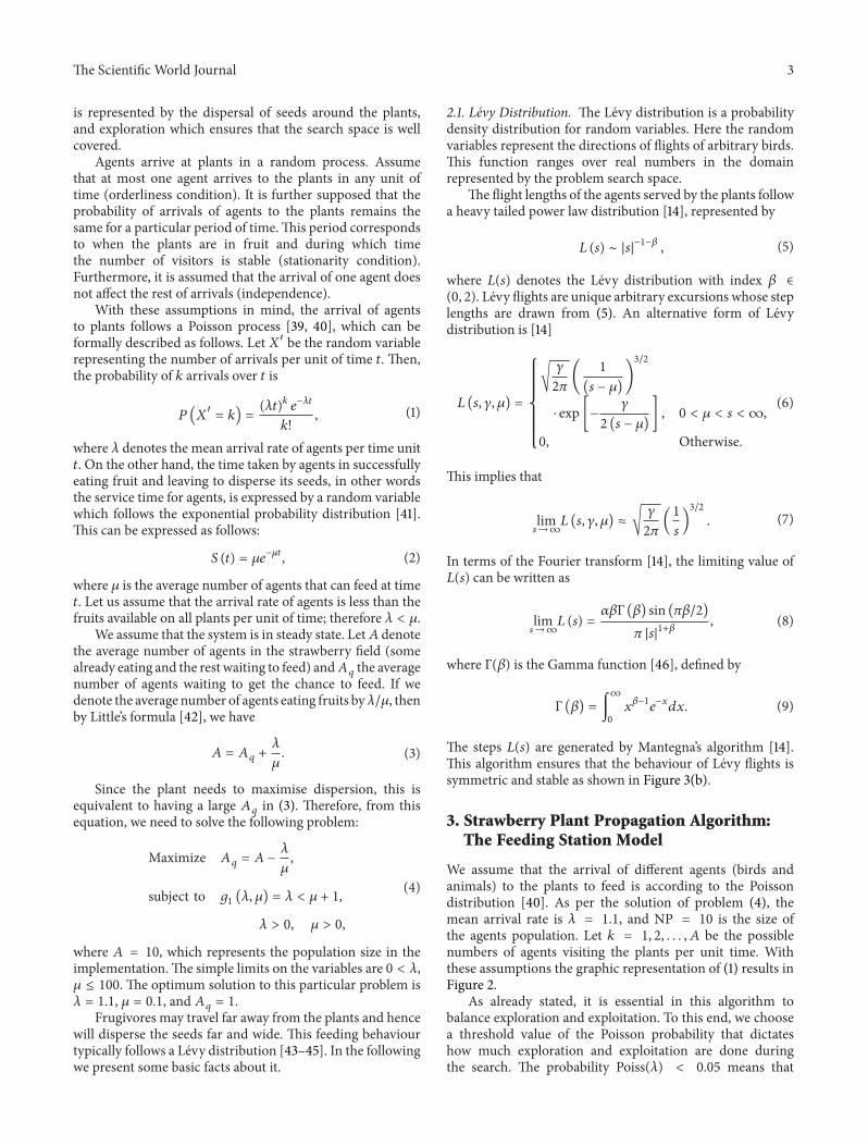
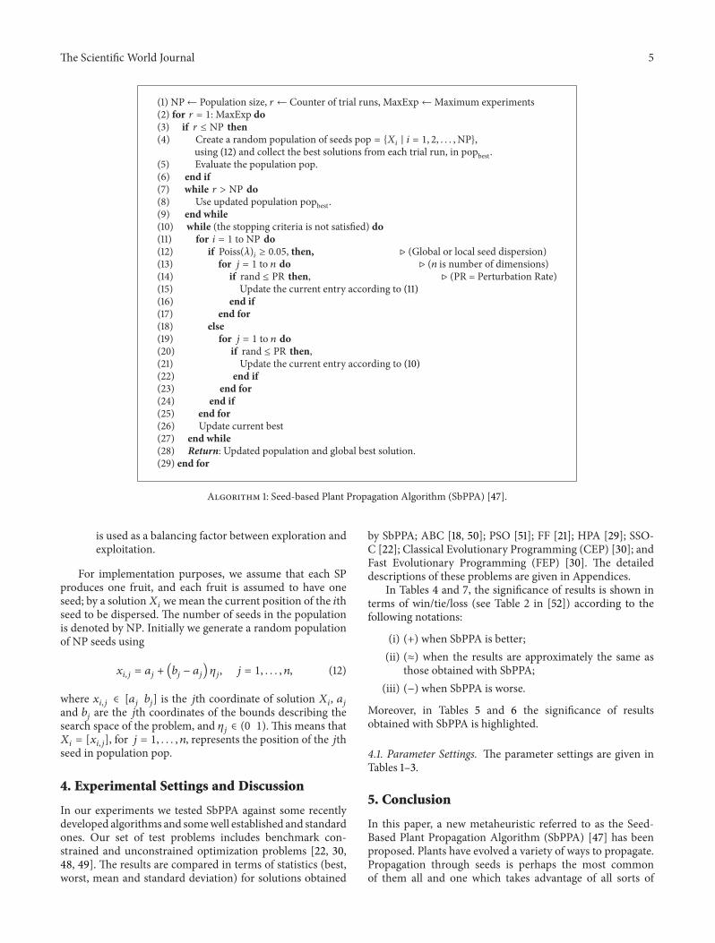
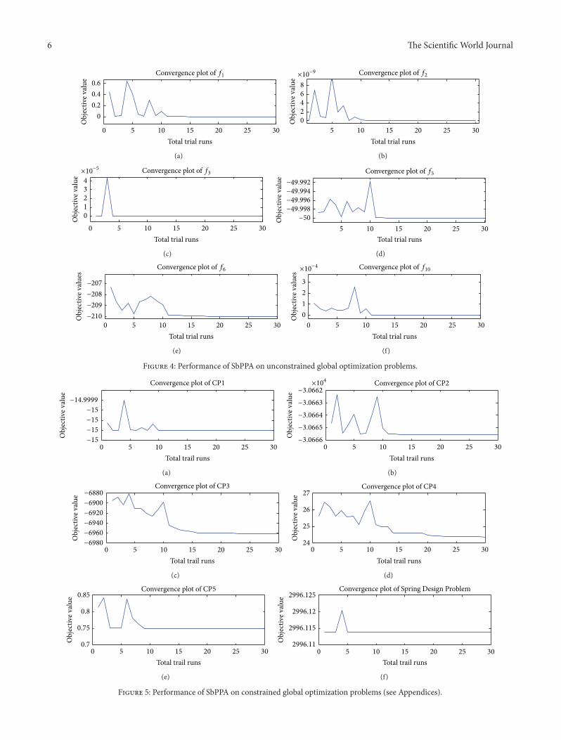
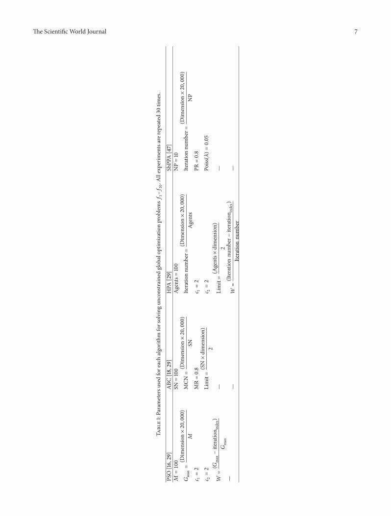
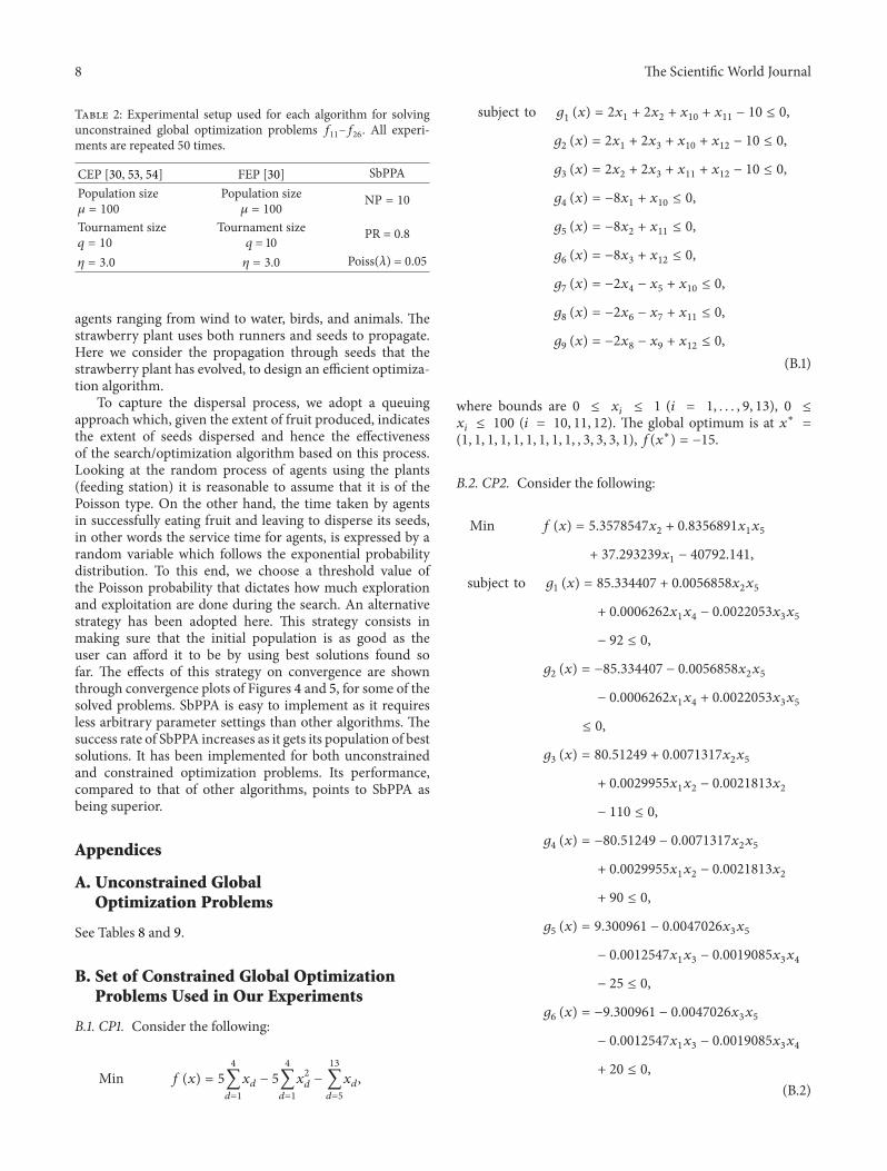
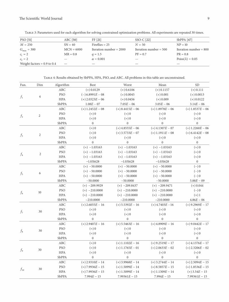
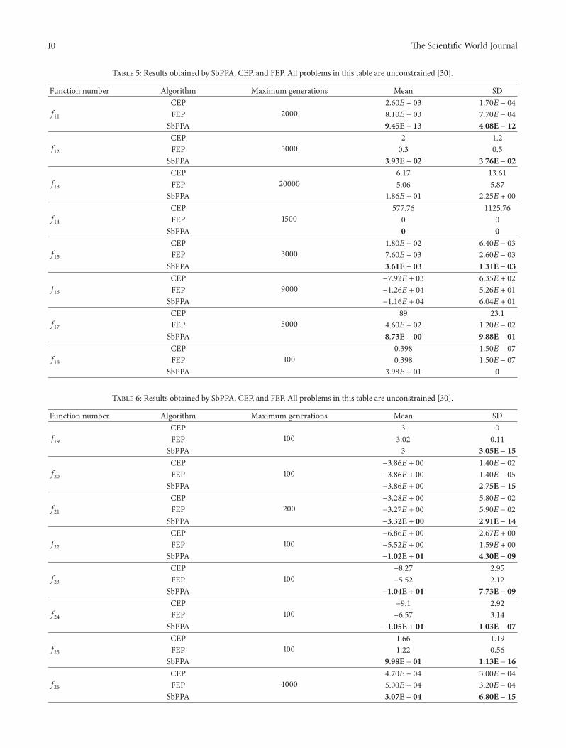
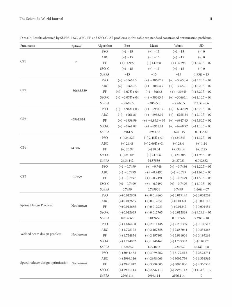
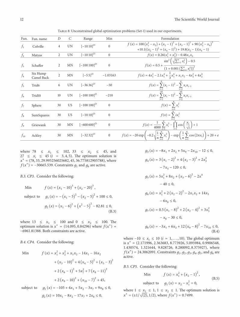
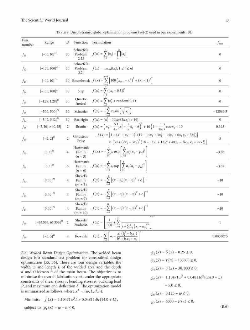
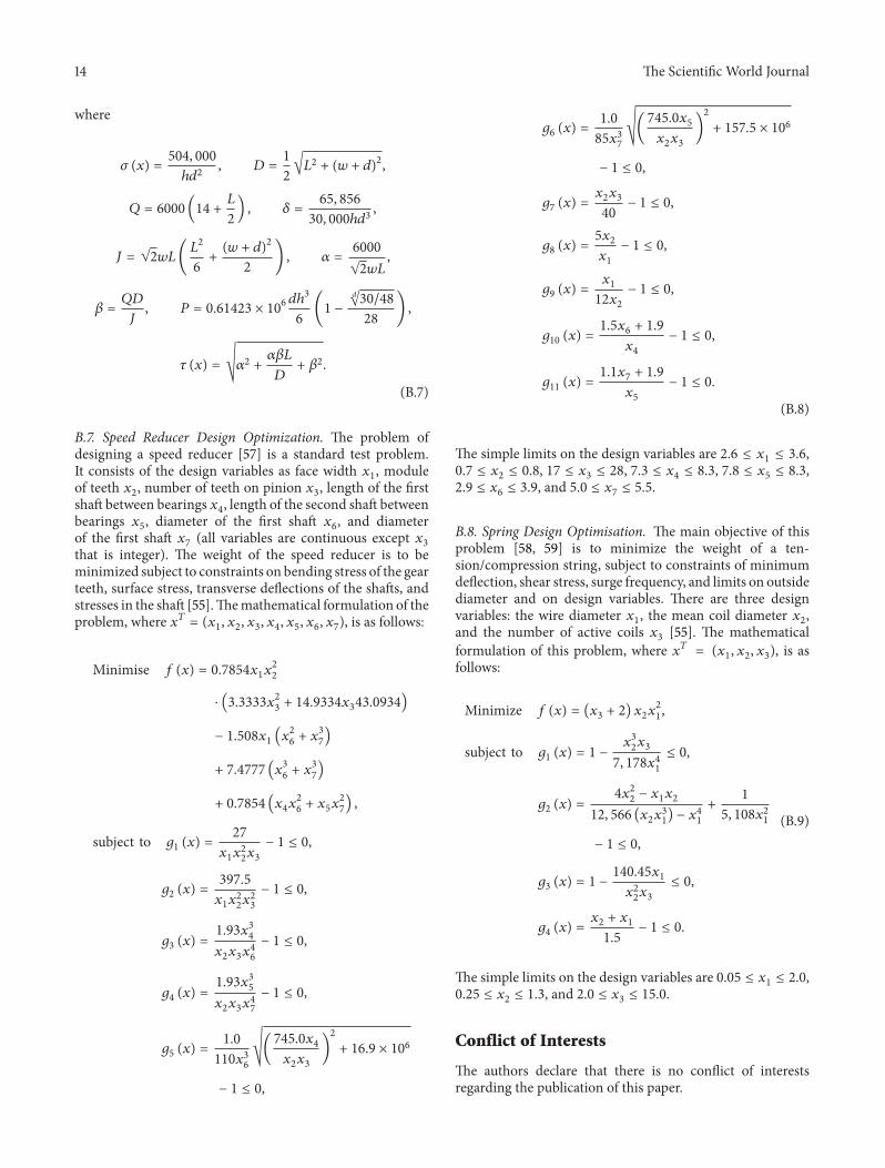
Related Documents


