A Schema for Constraint Relaxation with Instantiations …eil.utoronto.ca/wp-content/uploads/aac/papers/beck-msc.pdf · A Schema for Constraint Relaxation with Instantiations for

A Schema for Constraint Relaxation with Instantiations for

Partial Constraint Satisfaction and Schedule Optimization

by

John Christopher Beck

A thesis submitted in conformity with the requirements

for the degree of Master of Science

Graduate Department of Computer Science

University of Toronto

© Copyright J. Christopher Beck, 1994

2

iii

Abstract

A Schema for Constraint Relaxation with Instantiations for Partial

Constraint Satisfaction and Schedule Optimization

John Christopher Beck

Master of Science

Department of Computer Science

University of Toronto

1994

We investigate constraint relaxation within a general constraint model. We claim that a key torelaxation is recognition that a constraint can be modified in a variety of ways and that eachmodification potentially carries a different impact for both the quality of the solution and theproblem solving process. Our primary motivation is the application of constraint relaxation asa technique for coordination of multiple agents in a shared environment.

We propose a schema for constraint relaxation that is based on the propagation of informationthrough a constraint graph. The schema isolates five heuristic decision points where tech-niques of varying complexities can be specified. Three algorithms within the schema aredeclared and shown to perform well on Partial Constraint Satisfaction Problems (PCSPs).Three additional algorithms are defined and used in the estimation of the impact of schedulingdecisions in a medium size job shop scheduling problems. Difficulties with the calculation ofactual impact data prevents comparison among the algorithms. The algorithms represent anadvance by allowing propagation over all types of constraints and the ability to integrate heu-ristic decision making.

iv

v

Acknowledgments

I would like to thank all who made this work possible. In particular, I would like to expressgratitude to the following people:

To my parents, John and Anne, for love and support and for teaching me tothink.

To my supervisor, Mark Fox, for guidance and encouragement, as well as forunbelievably insightful comments.

To my second reader, Hector Levesque, for his useful comments

To Eugene Davis, Steve Green, John Chappel, Heather Hinton, Yaska Sankar,and Michael Gruninger for wading through early drafts and magnanimouslysacrificing both hours and red pens. I would especially like to thank Gene formany discussions about the research from its genesis to its apocalypse.

To Maureen Whelton, Monica Burchill, Helen Tubrett, Frank Beck, and NualaBeck for continually reminding me that there is a life outside of the lab and forkeeping me alive to experience it.

To Angela Glover, who demonstrated that the light at the end of the tunnel wasnot an oncoming train.

And finally to Nancy Bowes, who asked me to put her name here.

I would also like to acknowledge the financial support of the Natural Sciences and Engineer-ing Research Council and Digital Equipment Corporation.

vi

vii

Contents

Abstract iii

Acknowledgments v

Contents vii

List of Figures xi

List of Tables xiii

Chapter 1 Introduction 11.1 Constraint Relaxation Overview 11.2 Motivation 2

1.2.1 Coordination of Multiple Agents 21.2.2 Guiding Search with Relaxation 51.2.3 Scheduling 61.2.4 Constraint-Directed Reasoning 7

1.3 Constraint Satisfaction Problems (CSPs) 71.3.1 The CSP Model 71.3.2 CSP Algorithms 8

1.3.2.1 Retrospective Techniques 81.3.2.2 Prospective Techniques 101.3.2.3 Variable and Value Ordering 101.3.2.4 Texture Measurements 11

1.4 Constraint Relaxation 111.4.1 Relaxation as Repair and Optimization 121.4.2 Relaxation and Selective Non-Satisfaction of Constraints 12

1.5 Contributions of this Work 131.6 Plan of Dissertation 13

Chapter 2 Related Work 152.1 Probabilistic Labeling in Machine Vision 152.2 Non-Satisfaction of Constraints By Weight 162.3 Extending CSP Solving Methods 172.4 Constraint Optimization 19

2.4.1 Optimization in Operations Research 202.4.2 Optimization in Artificial Intelligence 21

2.5 Scheduling 222.5.1 Constructive Scheduling 222.5.2 Repair-based Scheduling 23

viii

2.5.3 Fuzzy Scheduling 232.5.4 Estimating the Impact of a Scheduling Decision 24

2.6 Discussion 262.7 Summary 27

Chapter 3 A Schema for Constraint Relaxation 293.1 Foundational Concepts 29

3.1.1 Constraint Model 293.1.2 Search With Relaxation 30

3.2 Relaxation-Based Search 303.2.1 Propagation 313.2.2 An Extended Example 323.2.3 Comments on the Example 36

3.3 The Relaxation Schema 363.4 Basic Propagation 38

3.4.1 Value and Cost Propagation 383.4.2 Relaxation Propagation 393.4.3 Termination of Propagation 40

3.5 Relaxation in Non-Trivial Graphs 413.6 Summary 42

Chapter 4 Cache-Based Constraint Relaxation 434.1 Difficulties With Cycles 43

4.1.1 Counting Cycle Costs 434.1.2 Relaxation Information 464.1.3 Complexity 48

4.2 Using Information Caches to Limit Search 484.2.1 Using Stored Costs 494.2.2 Bounding the Search 494.2.3 Enhancements 50

4.3 Cache-Based Relaxation Algorithms 514.3.1 Finding an Initial Solution 524.3.2 Single Min-Value Relaxation 524.3.3 Multiple Min-Value Relaxation 534.3.4 MinConflicts-like Relaxation 544.3.5 Complexity 54

4.4 Experiments with PCSPs 554.4.1 Partial Constraint Satisfaction Revisited 554.4.2 Partial Extended Forward Checking 55

4.5 Experiments 564.5.1 Evaluation Criteria 574.5.2 Problem Description 57

4.6 Results 584.6.1 Preliminary Experiments 584.6.2 Consistency Checks 594.6.3 Solution Cost 60

4.7 Discussion 614.7.1 Non-Uniform Relaxation Costs 61

4.7.1.1 Consistency Checks 61

ix

4.7.1.2 Solution Costs 624.7.2 Increasing the Number of Variables 624.7.3 Estimation of Global Cost vs. Local Cost 634.7.4 The MC Algorithm 64

4.8 Summary 65

Chapter 5 Relaxation-Based Estimation of the Impact of Scheduling Decisions 675.1 Estimating the Impact of a Scheduling Decision Revisited 675.2 Job Shop Scheduling 68

5.2.1 A Constraint Model for Job Shop Scheduling 685.2.2 Temporal Variables and Constraints 695.2.3 Resource Variables and Constraints 705.2.4 Example 715.2.5 Constraint Relaxation in Scheduling 725.2.6 Extending the Example 73

5.3 A General Relaxation-Based Algorithm for Cost Estimation 745.3.1 The General Estimation Algorithm 745.3.2 Finding a Subgraph 765.3.3 The Constructive Search Algorithm 77

5.3.3.1 Value and Control Propagation 775.3.3.2 Backtracking 785.3.3.3 The Relaxation Schema 78

5.3.4 Calculating the Cost of a Subgraph Solution 785.3.5 Partial Solutions vs. Solutions to the Subgraph 795.3.6 Complexity 80

5.4 The Cost Estimation Algorithms 805.4.1 The Depth Algorithm 805.4.2 The TemporalOnly Algorithm 805.4.3 The TopCost Algorithm 815.4.4 The Contention/Reliance Algorithm 815.4.5 Expectations 82

5.5 Experiments 825.5.1 Experimental Problems 835.5.2 Cost Model 835.5.3 Evaluation Criteria 855.5.4 The Source Activity 86

5.5.4.1 Selecting the Source Activity 865.5.4.2 Selecting Candidate Values for the Source Activity 87

5.5.5 The Depth Algorithm 875.5.6 Parameter Settings for the Texture-Based Algorithms 89

5.5.6.1 Subgraph Size 895.5.6.2 NumberOfSets and SetSize 895.5.6.3 Summary of Algorithm Variations 90

5.6 Results 915.6.1 Raw Data 915.6.2 Texture Measurements 935.6.3 Subgraph Size 955.6.4 Parameter Settings 975.6.5 Overall 98

x

5.7 Discussion 1005.7.1 The Depth Algorithm 1005.7.2 TopCost vs. Baseline 1005.7.3 Poor Performance of Contention/Reliance 1015.7.4 TopCost4 vs. TopCost10 1015.7.5 Reassessing the Estimations 102

5.8 Conclusion 1025.8.1 Building Practical Algorithms 102

5.9 Summary 103

Chapter 6 Coordination of Multiple Agents 1056.1 A Theory of Coordination 1056.2 A Mediated Approach to Coordination 106

6.2.1 The Role of the Mediator 1066.2.2 Why Mediation? 106

6.3 Supply Chain Management Revisited 1076.3.1 An Example 107

6.4 Conclusion 110

Chapter 7 Concluding Remarks 1137.1 Contributions 113

7.1.1 A Generalized Constraint Model 1137.1.2 A Schema for Relaxation Algorithms 1147.1.3 Three Relaxation Algorithms for PCSPs 1147.1.4 Application of the Relaxation Schema to Schedule Optimization 115

7.2 Future Work 1157.3 Summary 116

Bibliography 117

xi

List of Figures

Figure 1. The Material Flow in the Supply Chain of a Manufacturing Enterprise 3Figure 2. Logistics Level Scheduling of a Customer Order 4Figure 3. A Simple Activity/Resource Constraint Graph 5Figure 4. The Forward Step of the PEFC3 Algorithm [Freuder 92] 18Figure 5. A Simple Constraint Graph 32Figure 6. Snapshot of the Graph After Step 6 33Figure 7. Snapshot of the Graph After Step 14 34Figure 8. The Graph after All Value/Cost Propagation 35Figure 9. The Graph of the Final Solution for x1 = 2 35Figure 10. Pseudocode for Relaxation Propagation 39Figure 11. Redefinition of the PostCost Function to account for Graph Cycles 41Figure 12. A Constraint Graph with a Cycle 44Figure 13. A Close-up of the Constraint Graph in Figure 12 44Figure 14. A Constraint Graph with Cycles 45Figure 15. A Close-Up of a Subgraph from the Graph in Figure 14 45Figure 16. Overwriting the Cost Cache at a Constraint 47Figure 17. A Graph Corresponding to the Worst-Case Space Complexity of the

Context Mechanism 48Figure 18. Filtering the Cost Bound at a Variable 49Figure 19. Filtering the Cost Bound at a Constraint 50Figure 20. Pseudocode for the Main Loop of the Cache-Based Relaxation

Algorithms 51Figure 21. The Forward Step of the PEFC3 Algorithm 56Figure 22. Comparison of the Number of Consistency Checks for SMV, MMV, and

PEFC3 Algorithms 59Figure 23. Percentage Difference from Optimal Costs for SMV and MMV

Algorithms 60Figure 24. Schematic Diagram of The Activity Representation 69Figure 25. A Simple Precedence Constraint Between 2 Activities 70Figure 26. A Representation of Two Allen Relations with TemporalConstraints 70Figure 27. Schematic Diagram of The Activity Representation 71Figure 28. Constraint Representation of a Simple Job Shop Scheduling Problem 72Figure 29. Optimization Constraints on the Example Scheduling Problem 73Figure 30. Flow Chart of the General Estimation Algorithm 75Figure 31. The Average Cost Found by the Depth Algorithm with L = 1 for the

Problem Sets with 1 Bottleneck 87

xii

Figure 32. The Average Cost Found by the Depth Algorithm with L = 1 for theProblem Sets with 2 Bottlenecks 88

Figure 33. Raw Data for Problem 3, Problem Set 2 91Figure 34. Raw Data for Problem 1, Problem Set 5 92Figure 35. Raw Data for Problem 9 in Problem Set 8 92Figure 36. The EstGap Statistic for Estimations using Different Texture

Measurement 93Figure 37. The ChangeActivity Count Estimations using Different Texture

Measurement 94Figure 38. The Effect of Subgraph Size on the EstGap Statistic 96Figure 39. The Effect of Subgraph Size on the ChangeActivity Count 96Figure 40. The Effect of Parameter Settings on the EstGap Statistic 97Figure 41. The Effect of Parameter Settings on the ChangeActivity Count 98Figure 42. The Best EstGap Statistic for Each Texture Measurement and Subgraph

Size 99Figure 43. The Lowest ChangeActivity Counts for Each Texture Measurement and

Subgraph Size 99Figure 44. Logistics Level Constraint Graph of the Example 108Figure 45. Logistics Level Constraint Graph After Relaxation 110

xiii

List of Tables

TABLE 1. Variations of the SMV algorithm 53TABLE 2. Variations of the MMV algorithm 53TABLE 3. Variations of the MC algorithm 54TABLE 4. Parameters of the Experimental Problems 57TABLE 5. Average Number of Constraints and Average Optimal Cost for each

Problem Set 63TABLE 6. Variations of the Cost Estimation Algorithms 90TABLE 7. Current Schedule in the Supply Chain Simulation 108TABLE 8. Schedule After Relaxation 109

xiv

1

Chapter 1 Introduction

Constraint relaxation is the modification of the valid relationships among a set of variables ina constraint-based representation of a problem. The modification changes the problem defini-tion, allowing a superset of the original solutions. Its chief application is where finding a solu-tion to the original problem is prohibitively expensive or infeasible. Relaxation has thepotential for a much larger role in constraint-based search and reasoning than it has played tothis point. We are motivated by applications in guiding general constraint satisfaction, sched-uling, and coordinating autonomous agents. In this dissertation, we propose a schema for con-straint relaxation based on the propagation of information through a constraint graph.

This chapter presents an informal description of constraint relaxation and examines our moti-vation. We then present the necessary background on the constraint satisfaction techniquesfrom which some of the constraint relaxation techniques are evolved. Finally, we present adefinition of constraint relaxation and contrast it to similar notions appearing in the literature.

1.1 Constraint Relaxation Overview

Constraint-based techniques represent problems as a set of variables and a set of constraints.Each variable has a domain of possible values and each constraint limits the values that a sub-set of the variables can take on. A constraint is the embodiment of a particular relationshipamong a set of variables. A simple example of a constraint-based representation is used in thegraph coloring problem [Garey 79] . Each variable can be assigned a color from a limitedspectrum and each constraint defines that a particular pair of variables can not have the samecolor. The variables in a pair that is so limited are directly connected by a constraint or, equiv-alently, are adjacent variables. Adjacency is specified in the problem definition. The goal inconstraint satisfaction problems (and graph coloring, in particular) is to assign values (specificcolors) to variables such that all constraints are satisfied; that is, so that the relationshipdefined by each the constraint holds. As reviewed below, the typical solution techniquessearch via the systematic assignment of values to variables.

Constraint relaxation modifies the relationship defined by a constraint. As the term “relax-ation” implies, the modification allows a wider range of relationships. In graph coloring, forexample, we might decide that a particular adjacent variable pair can be different colors or canboth be red. This highlights the difference between relaxation of a constraint and non-satisfac-tion. Relaxation makes a particular change in the definition of the constraint (e.g. allowingboth variables to be red), whereas non-satisfaction removes the constraint completely: there is

2

no limit on the values to which the variables can be assigned.1 Once a constraint is relaxed,the problem is altered because a relationship that was not allowed in the original problem isnow acceptable.2

There has been some work on the selective non-satisfaction of constraints [Freuder 92] , andother work that can be interpreted as making contributions toward relaxation [Rosenfeld 76][Dechter 90] . A well-grounded theory is lacking. Such a theory has wide applications to anyproblem expressible in the constraint satisfaction paradigm.

1.2 Motivation

Constraint relaxation is applicable in two general areas. The first is in guiding search for asolution to an original problem. If we relax the problem, we may be able to use the easilyfound solutions to focus the search in the original problem. Secondly, relaxation is necessaryin overconstrained situations, where it is impossible to assign values in such a way that allconstraints are satisfied.

Our chief motivation for this work is the use of constraint relaxation as a coordination mecha-nism in multiagent domains. We plan to investigate coordination in the domain of the supplychain for a manufacturing enterprise. We have a number of additional motivations in the areasof guidance of general search, scheduling, and a theory of constraint-directed reasoning.

1.2.1 Coordination of Multiple Agents

Our foremost interest in constraint relaxation is in its use as a mechanism for efficient cooper-ation among a group of autonomous, resource-sharing, problem solving agents as they attemptto meet their own and group ends. This area of multiagent coordination has received a greatdeal of interest in the field of Distributed Artificial Intelligence [Distributed 87] [Distributed89] . We have adopted supply chain management as the focus of our work in coordinationbecause of the close mapping between the departments and actors in the supply chain andagents in a shared software environment. This mapping is seen in the fact that departmentswithin an enterprise work towards both global and local goals with shared, finite resources.Furthermore, often departments must work together to achieve these goals. We use the supplychain, here to highlight many of the challenges surrounding the coordination of agents.

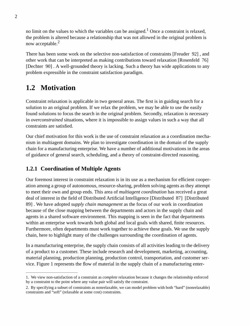
In a manufacturing enterprise, the supply chain consists of all activities leading to the deliveryof a product to a customer. These include research and development, marketing, accounting,material planning, production planning, production control, transportation, and customer ser-vice. Figure 1 represents the flow of material in the supply chain of a manufacturing enter-

1. We view non-satisfaction of a constraint as complete relaxation because it changes the relationship enforcedby a constraint to the point where any value pair will satisfy the constraint.

2. By specifying a subset of constraints as nonrelaxable, we can model problem with both “hard” (nonrelaxable)constraints and “soft” (relaxable at some cost) constraints.

3

prise. The diagram shows one aspect of the supply chain, leaving out a number of functions aswell as a representation of the flow of information and feedback. Figure 1 illustrates that thesupply chain is a complex interaction of a number of functional entities in order to achievesome level of performance in the delivery of products to customers.

Figure 1. The Material Flow in the Supply Chain of a Manufacturing Enterprise

Each link in the chain is subject to unexpected events, and quick response to these events is akey element in the success and survival of a corporation [Nagel 91] . Exogenous events aremany and varied: change in the customer order, late delivery or price change of a particularresource, machine breakdown, an urgent order from a good customer, and so on. Handlingthese events requires close coordination and cooperation among all departments in the enter-prise. The following example illustrates the scope of the problem [Fox 92] .

The Canfurn, Inc. furniture company produces furniture with various options. Leo’s, the larg-est and best-paying customer of Canfurn, places a large order for delivery in six months andCanfurn schedules delivery. Two months before the original delivery date, Leo’s requests asignificant change in the order but wants to maintain the same delivery date. Canfurn’s salesdepartment immediately contacts the manufacturing division. Manufacturing has a number ofoptions and a number of questions that need to be answered:

• Manufacture the modified order. Can the new order be manufactured? Are extra shiftsneeded? What does personnel think of extra shifts? Are the raw materials in stock? If not,can a supplier be found?

• Delay another order. Can another order be delayed (and delivered late) in order to meetLeo’s order? What does sales think?

Suppliers Customers

WarehousesFactories

4

• Subcontract the job to another manufacturer. Can the job be subcontracted? What doesmarketing and strategic planning think? What does accounting say about reducing the mar-gins? Can we afford to take a loss on the order?

Clearly, the manufacturing division cannot make the decision independently. It must canvas anumber of other divisions within the company and some external bodies (suppliers and sub-contractors) in order to choose an alternative that is as inexpensive as possible.

The Enterprise Integration Laboratory at the University of Toronto is developing an IntegratedSupply Chain Management System (ISCM) addressing these and other problems. The projectis based on a distributed simulation of an enterprise, where departments are encapsulated assoftware agents. Given this distribution, the inter-departmental coordination in real corpora-tions is manifest in the inter-agent coordination in the simulation.

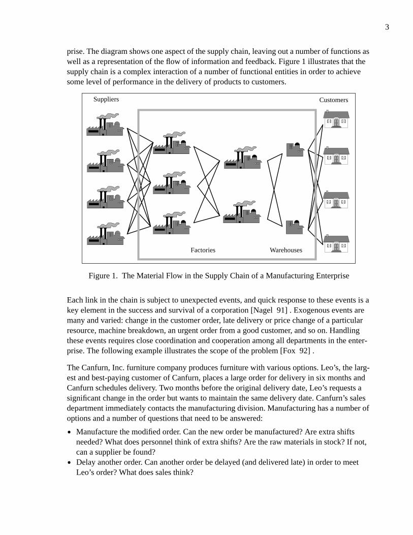
The inter-agent coordination is hierarchical. With multiple production centers (e.g. factories),coordination among agents within one center is a level of abstraction below the coordinationamong the centers. The latter abstraction represents enterprise-wide logistics. It has a globalview of the enterprise and is concerned with sales, delivery to the customer, and all aspects ofinter-production-center coordination.

Figure 2. Logistics Level Scheduling of a Customer Order

Each production center is viewed as a single resource with the ability to perform multipleactivities resulting in the production of a quantity of a resource. The activities each factory canperform and the capacity of each factory is known.3 Logistics-level scheduling assigns facto-ries to supply specific quantities of resources at particular times.4 The factories commit tothese assignments. Figure 2 shows a schematic of the logistics-level assignments when an

OrderAcquisitionOrder from

Customer

Factory1 Factory2 Factory3

Produce: RESBQuantity: Q2Time: T2Using: RESA

Produce: RESAQuantity: Q1Time: T1

Produce: PRODQuantity: Q4Time: T4Using: RESC

Produce: RESCQuantity: Q3Time: T3Using: RESB

LogisticsAgent

5

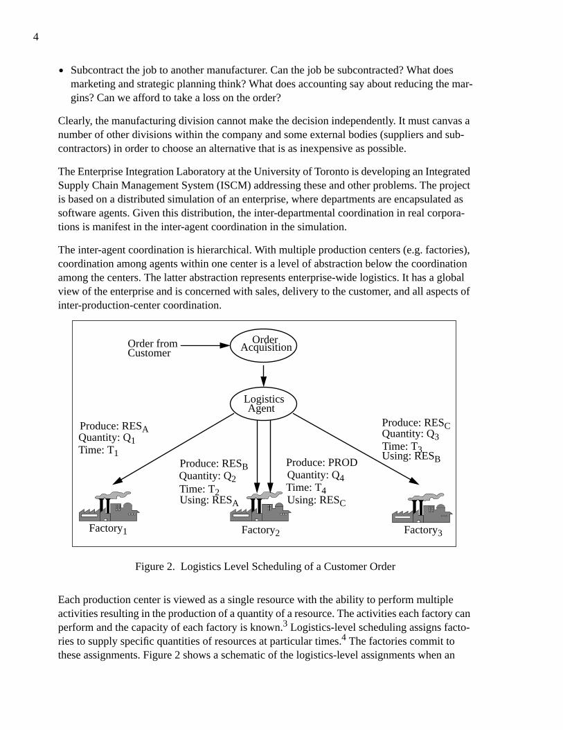
order is received via the Order Acquisition agent. On the basis of these commitments, activi-ties at other production centers are scheduled. This results in a commitment graph of inter-dependent activities such as shown in Figure 3.

Figure 3. A Simple Activity/Resource Constraint Graph

With the occurrence of an unpredicted event, it is likely that factories will not be able to meetall their commitments. In these infeasible situations, it is necessary to assess the alternativesand adopt the one with a small negative global impact. The commitment graph must be recon-figured to escape an overconstrained situation: this is constraint relaxation. Given multipleorders and activities at each factory, a full constraint graph will certainly grow to a non-trivialsize. A search for a near-optimal reconfiguration has to handle the combinatorial explosion ofinterdependent alternatives in resource choice, transportation method, and execution times, toname just a few. We believe that constraint relaxation guided by structural properties of thecommitment graph can be applied to this problem.

1.2.2 Guiding Search with Relaxation

Problem solving can be guided by solutions to related, simpler problems. This technique hasbeen used in the Operations Research community in the branch-and-bound technique [Hillier80] [Cplex 92] . The solution space is partitioned based on a bound on the optimization func-tion. The bound is found by solving a problem that ignores several of the original constraints.Portions of the solution space are selected and further partitioned based on assertion of one ofthe original constraints. Iteration continues until all constraints have been asserted and a solu-tion is found or it is found that no feasible solutions exists.

3. These capacities represent aggregate information based on previous performance. Environmental events (e.g.machine breakdown) can dynamically impact these capacities.

4. For now, we ignore the scheduling of the transportation between factories and the delivery to the customer,though this is included in the scope of the ISCM project.

ACT0

RESA RESB

RESC

Produce Use

PROD

Factory1 Factory2 Factory3

ACT1

ACT3

ACT2

Customer

6

The ISIS scheduling system uses constraint relaxation to rate a number of competing partialschedules [Fox 87] . Based on the rating that reflects the relaxation necessitated by the partialsolution, a subset of the solutions are selected for extension.

It has been shown that the shape or topology of the constraint graph has significant effect onthe efficiency of the search for a solution. In particular to ensure a linear time search, the graphmust be tree-shaped [Freuder 85] . The ABT algorithm is created to exploit this condition[Dechter 88] . ABT finds the minimum spanning tree of the full constraint graph and exhaus-tively generates solutions to the spanning tree graph. The number of solutions that each valuein the domain of a variable takes part in is used to guide the value ordering for subsequentsearch through the full constraint graph.

Using solutions to a relaxed problem to guide search of the full graph is intriguing. Each of theabove examples uses solutions to relaxed problems to expedite search in the full problem. Afirm theory of constraint relaxation may point toward relaxation schemes that produce easilysolved problems in many different problem solving contexts.

1.2.3 Scheduling

Scheduling is a difficult task that can be formulated using a constraint representation. Reasonsfor scheduling difficulty include [Fox 90a]:

• Scheduling is a constrained optimization problem over such criteria as tardiness, processtime, inventory time, and cost. The problem space can be very large.5

• Many scheduling problems are overconstrained due to the unavailability of resources giventhe temporal constraints (e.g. due dates, release dates, and precedence constraints).

• Constraint representations have failed to stress the importance of domain values. The num-ber and identity of tasks that require a resource over a particular time interval is a key pieceof information that can form the basis for heuristic variable and value orderings.

Underlying these difficulties is the fact that many of the constraints in scheduling are disequal-ity constraints (e.g. two tasks cannot use the same resource at the same time). Disequality con-straints create the large search space that may have few (or no) satisfying solutions and makenecessary the close attention to domain values.

That scheduling is actually a constrained optimization problem makes it a candidate for relax-ation. If the optimization criteria are explicitly represented by relaxable constraints, scheduleoptimization is equivalent to finding a low cost relaxation of the optimization constraints. Fur-thermore, since scheduling problems are often overconstrained, relaxation is sometimesneeded to find any solution, not just optimized solutions.

5. For example, a 100-activity problem, with 100 time slots and 100 resources has a search space of 10400 [Fox90a].

7

1.2.4 Constraint-Directed Reasoning

A further motivation for addressing constraint relaxation is the belief that constraints have alarge role in heuristic problem solving. A theory of constraint-directed reasoning pointstoward constraints and the constraint graph structure as the main features in search. The ISISsystem [Fox 86] [Fox 87] uses a rich constraint representation in extending the heuristicsearch paradigm to include constraint-directed reasoning. Not only do constraints defineadmissible solutions, but also they establish a partial ordering among those solutions, generatealternate search states, and provide a structure for the problem solving knowledge. [Fox 86]presents eleven observations of the role of constraints in problem solving. These roles includestate-generation, parameterization of the search space, providing the contextual relevance ofan operator, and stratification of both the representation and the search.

Relaxation is an important component of any theory of constraint-directed reasoning. In ISIStwo modes of relaxation are used: analytic and generative. Analytic relaxation chooses con-straint alternatives on the basis of an examination of the current state of the search. Generativerelaxation uses constraint alternative choices as an operator to produce a new search state. Forrelaxation to play such roles, a firm semantics is needed to assess why and how a relaxationshould be done. A range of tools that can be applied in both analytic and generative relaxationto suggest appropriate relaxations given the problem solving context is also required.

1.3 Constraint Satisfaction Problems (CSPs)

Before presenting a definition of constraint relaxation, we review the constraint satisfactionliterature upon which constraint relaxation is based. In this section, we will present the typicalconstraint satisfaction model and discuss solution techniques.

1.3.1 The CSP Model

The general CSP consists of the following:

• A set of n variables {x1, …, xn} with values in the discrete, finite domains D1, …, Dn.• A set of m constraints {c1, …, cm} which are predicates ck(xi, …, xj) defined on the Carte-

sian product Di × … × Dj. If ck is TRUE, the valuation of the variables is said to be consis-tent with respect to ck or, equivalently, ck is satisfied.

A solution to a CSP is an assignment of a value to each variable from its respective domainthat satisfies all constraints. In the basic CSP, all solutions are equally rated.

8

The most common conceptualization of a CSP is as a graph with variables represented bynodes and constraints by arcs.6 The graph structure leads to the notion of traversal of con-straints and of “transmitting” information between variables over the constraint links. Thistransmission is called propagation. Propagation is an important mechanism in the relaxationalgorithms presented in this dissertation.

The constraint model has proven to be a general problem solving structure employed in manyareas. The following is a partial list of areas where the constraint formalism has been applied(adapted from [Kumar 92] ). It reflects the broad applicability of the constraint-basedapproach to problem solving:

• Planning [Descotte 85] [Conry 86] [Lansky 88] [Conry 91] [Pope 92] .• Scheduling [Fox 87] [Fox 89] [Sadeh 91] [Ijcai 93] [Davis 94] .• Truth-maintenance [Huhns 91] .• Machine vision [Waltz 75] [Rosenfeld 76] [Shapiro 81] .• Temporal reasoning [Allen 83] .• Graphical user interfaces [Borning 87] .• Logic programming [Borning 88] [Van 89] .• Configuration [Mittal 90] .• Abduction and induction [Page 91] .• Design [Navinchandra 87] [Navinchandra 91] .• Enterprise modeling and design [Gruninger 94] .

1.3.2 CSP Algorithms

CSPs are amenable to generate-and-test algorithms where all possible value assignments aresystematically evaluated. On average, however, more efficient search can be achieved whenthe variables are instantiated sequentially in some order. We follow [Freuder 92] in dividingthe sequential solution techniques into retrospective and prospective flavours. An excellentsurvey of CSP solving is presented in [Kumar 92] .

1.3.2.1 Retrospective Techniques

Retrospective techniques are characterized by the assignment of a value to a variable followedby testing against variables that are already assigned. If all constraints are satisfied, anothervariable and value are selected. If some constraint is not satisfied, backtracking occurs. Back-tracking reassigns one of the variables to another value in its domain. If all values in thedomain of a variable have been unsuccessfully tried, the variable is left unassigned and back-tracking moves to another variable.

6. Other conceptualizations exist, including the dual constraint graph and join graph [Dechter 90] . In general, aconstraint graph is a hypergraph with arcs connecting all relevant nodes.

9

The simplest retrospective technique is chronological backtracking. If the compatibility checkfails, another value is tried for the most recently assigned variable. If all values in the domainof the variable are unsuccessfully tried, the variable is left unassigned and a new value isassigned to the next-most recently assigned variable. The gain over generate-and-test comeswhen an incompatibility is found amongst a subset of variables before all variables are instan-tiated. That part of the search space is pruned because there is no possibility of a solution.

Chronological backtracking suffers from a number of problems, in particular inefficientbehaviour known as thrashing [Mackworth 77] [Kumar 92] . Thrashing occurs when thesearch fails in multiple places for the same reason. If all the values for a variable fail, chrono-logical backtracking returns to the most recently instantiated variable. It is possible, however,that the reason for failure is an inconsistency with a variable much further back in the searchtree. A great deal of instantiation and backtracking will be done on the intervening variablesbefore the value of the offending variable is changed. If more effort is expended on finding thecause of the failure, some of this wasted work may be avoided.

In both backjumping [Gaschnig 77] and backmarking [Gaschnig 78] information is cached ateach variable to aid in the more precise identification of the offending variables. Instead ofreturning to the next-most recently assigned variable upon a failure, a number of variables arebacktracked through at one time to find the offending variable. Search is significantly reducedby avoiding instantiating the value combinations of the intervening variables. The differencein the two methods is the amount of information kept at each variable. Backmarking storesmore information and so is more efficient in terms of the number of compatibility checks itneeds to do. Because backmarking requires storage of a larger amount of information at eachvariable, the space complexity is better for backjumping.

An additional inefficiency in backtracking is the performance of redundant work. For exam-ple, consider two variables, xa and xb, that are widely separated in the variable ordering yetshare a tight constraint. If there is a complex relationship amongst the intervening variables, anon-trivial amount of work is done in discovering this relationship. If the tight constraintcauses a failure at xb, backtracking will return to xa. The relationship amongst the interveningvariables must be re-discovered when search proceeds forward with a new value for xa. Chro-nological backtracking, backmarking, and backjumping suffer from this fault because theyuninstantiate intervening variables when returning to the failure-causing variable. Depen-dency-directed backtracking addresses this problem [Stallman 77] [Kumar 92] . In general,when an inconsistency is found, it is recorded and used as a justification for a new assignment.If backtracking occurs past these variables, the justifications still exist and an assignment canbe made without recapitulating the previous search. If dependency-directed backtracking isfully implemented all redundant work is avoided. The complexity of finding and maintainingthe justifications is so high, however, that often dependency-directed backtracking performsworse than chronological backtracking [Kumar 92] .

10

1.3.2.2 Prospective Techniques

In contrast to retrospective techniques, prospective CSP solvers propagate the effects of avariable instantiation to unassigned variables. This propagation is based on three consistencyalgorithms that grew from a recognition of three reasons for thrashing [Mackworth 77] . Thefirst reason is lack of node consistency: when elements in a variable’s domain do not satisfyunary constraints. Assigning these values causes immediate failure. However when a non-node consistent variable is backtracked over and re-tried, the same failures will occur again.The second reason, lack of arc consistency, applies the same concept to binary constraints. Ifthe value of one variable has no consistent counterpart in the domain of a directly connectedvariable, failure will eventually occur. When the two variables are far apart in the order ofinstantiation a great deal of work is done and no failure occurs until the latter variable isreached. This work is repeated multiple times until the backtracking finally returns to the firstvariable. Finally, a lack of path consistency is also a source of thrashing. With three variables,xi, xj, and xk, where each shares a constraint with the other two, it is possible that for some pairof values for (xi, xj) there is no consistent value for xk. This creates behaviour similar to thatseen with lack of arc consistency. Consistency algorithms [Mackworth 77] have been definedthat establish each of these conditions by the propagation of domain values across constraints.Unfortunately, except in special cases [Freuder 85] , establishing all or any of these forms ofconsistency does not guarantee a backtrack-free search. Prospective algorithms work byestablishing some form of consistency after every variable instantiation.

The most common form of prospective algorithm is forward checking [Haralick 80] [Shapiro81] . The algorithm instantiates a variable, x, and prunes inconsistent values from the domainsof adjacent variables. If any of the domains become empty, failure occurs, and x must be re-assigned. When backtracking, care must be taken to return the domains to the state prior to thepruning. Early in the search, forward checking does more consistency checks than a retrospec-tive algorithm, however, when domains have been pruned, many fewer consistency checks areperformed.

If establishing some level of consistency is useful, it may be worthwhile to create a more fullyconsistent graph. Experiments comparing backtracking searches with different consistencyalgorithms between variable instantiation steps have been run [Nadel 88] [Kumar 92] .Results indicate that it is often better not to establish full consistency since the effort investedin achieving consistency can be greater than that necessitated by the additional backtracking.7

1.3.2.3 Variable and Value Ordering

In a backtracking search, significant performance changes can result from a modification tothe order in which variables are instantiated and/or values are tried at each variable [Kumar92] . In a CSP that has a satisfying solution, a perfect variable/value order would produce alinear time solution because no backtracking would be necessary. The most common heuristic

7. But see [Nuitjen 93] for some interesting evidence to the contrary in the scheduling domain.

11

is to instantiate the most constrained variable to its least constraining value. Intuitively, byinstantiating the most constrained variable earlier, backtracking will take place earlier andthrashing can be minimized by pruning the search space. By assigning the least constrainingvalue, the likelihood of finding a solution without having to backtrack to this variable isincreased. Reliable identification of critical variables and values is an open research question.

1.3.2.4 Texture Measurements

None of the presented problem solving techniques escape a worst-case exponential search. Asa consequence, it is important to make good heuristic search decisions in solving practicalproblems. In particular, texture measurements [Fox 89] can be used as a basis for heuristicdecisions. A texture measure is an assessment of properties of a constraint graph reflecting theintrinsic structure of a particular problem. Examples include variable and constraint tightnessand constraint reliance. Texture measures have been used in the job shop scheduling domain[Sadeh 91] as a basis for opportunistic variable and value ordering decisions.

A goal of research on texture measures is to find correlations between particular graph struc-tures and performance of an algorithm [Fox 89] [Davis 94] . If such correlations can befound, the search algorithm could be automatically configured based on texture measure-ments. Such general results have not yet been shown.

1.4 Constraint Relaxation

Constraint relaxation is the modification of the meaning of a constraint that changes the rela-tionship that it enforces among a subset of problem variables. Given the usual CSP model,relaxation of constraint, ck, changes the predicate ck(xi, …, xj), resulting in the predicate hav-ing a value of TRUE for larger subset of the Cartesian product of the relevant variables.

Because constraint relaxation changes the problem definition, a solution to a problem withsome relaxed constraints is different from a solution to the original problem. We represent thisdifference by specifying that a cost is incurred when a constraint is relaxed. This cost dependson the specific modification that is performed because a constraint can be relaxed in numer-ous ways. The specific relaxation that is performed has significant impact on both the localcost of the relaxation and on its utility in later search.

A solution to a constraint relaxation problem is the assignment of values to variables and therelaxation of some constraints so that all constraints are satisfied and the cost is as small aspossible.

12

1.4.1 Relaxation as Repair and Optimization

We have two views of constraint relaxation:

1. Relaxation is an operator in repair-based search. When a partially consistent solution existsfor a CSP, we can easily find a solution to the relaxed problem by relaxing the constraintsthat are not satisfied. An attempt is made to minimize the cost by relaxing some constraintsand changing some values. Relaxation can significantly expand the solution space of aproblem and lead to subsequent search based on CSP techniques.

2. Relaxation is a form of optimization. We can model the optimization criteria as a set ofrelaxable constraints representing the sole source of cost in the problem.

These two views of relaxation are not incompatible. Especially in the scheduling domain,relaxation allows the modeling of problems where not only are there optimization criteriasuch as tardiness, but there are also options and trade-offs involved with problem constraints.

1.4.2 Relaxation and Selective Non-Satisfaction of Constraints

Selective non-satisfaction of constraints ignores some of the problem constraints in order tomake the problem easier to solve. Ignoring a constraint means treating it as if it does not exist:it no longer places any limit on the relationships among the variables. We saw this in the ABTalgorithm where all the constraints that were not in the minimum spanning tree of the graphare ignored. Non-satisfaction of constraints is also the main mechanism behind Partial Con-straint Satisfaction Problems (PCSPs) [Freuder 92] . The goal in PCSPs is to find a valuationfor the variables that satisfies as many constraints as possible.

Algorithms based on selective non-satisfaction of constraints fail to represent the semanticcontent of constraint relaxation. There are many ways to relax a constraint and each relaxationcan have different effects on the relationship of the relaxed problem to the original. For exam-ple, in a scheduling problem, choosing to ignore a due date constraint may lead to a simplesolution to the rest of the problem. However, relaxation of a due date constraint by 3 hours hassignificantly less impact than relaxation of the constraint by 3 days. Non-satisfaction of a con-straint misses this point because it does not represent the difference between a relaxation of 3hours and a relaxation of 3 days.

Despite the fact that non-satisfaction of constraints does not represent the key semantic issues,it is a special case of constraint relaxation. In our model of constraint relaxation, the functionthat finds the cost of a relaxation of a constraint can be specified. We can define that the cost ofall relaxation of all constraints is equal and therefore model non-satisfaction of constraints.

13

1.5 Contributions of this Work

The contributions of this dissertation are fivefold:

1. A generalization of the constraint model that allows generation of alternative constraintsand an assessment of their local impact. This generalization represents the semantic mean-ing of relaxation by defining the cost of relaxation to be based on the constraint itself andon how relaxation is done. The ability to generate and assess alternative constraints is a sig-nificant addition to general constraint techniques.

2. A flexible relaxation schema within which relaxation techniques can be specified andinvestigated. The schema is applicable to all types of constraints and is modulated by heu-ristic decisions specified at the time of instantiation.

3. A specification of three relaxation algorithms shown to perform well on Partial ConstraintSatisfaction Problems (PCSPs). These algorithms demonstrate the applicability of algo-rithms defined within the schema to repair-based search on general constraint graphs.

4. The application of propagation techniques and texture-based heuristics within the relax-ation schema to schedule optimization. We model the sources of cost in schedule optimiza-tion with relaxable constraints. Three schema-based algorithms are defined which assessthe impact of scheduling decisions by estimating the relaxation necessitated by the deci-sion.

5. The modeling of multiagent coordination as a problem requiring constraint relaxation. Werepresent the interactions among agents as a shared constraint graph, and therefore, a situa-tion requiring coordination is manifest by the need to re-establish feasibility in this con-straint graph. Relaxation is a technique to re-establish graph feasibility.

1.6 Plan of Dissertation

In Chapter 2, we review the literature relevant to constraint relaxation. We present our propa-gation-based relaxation schema in Chapter 3. Three instantiations of the relaxation schema forPartial Constraint Satisfaction Problems (PCSPs) are specified and empirically evaluated inChapter 4. In Chapter 5, we turn to relaxation for schedule optimization. We describe the jobshop schedule optimization problem and present three algorithms for the estimation of theimpact of scheduling decisions. Chapter 5 also presents empirical results comparing the esti-mations made by our algorithm to baseline estimates. In Chapter 6, we return to the domain ofmultiagent coordination and discuss the relevance of the relaxation techniques developed inthis dissertation. Finally, in Chapter 7, we conclude and a look at prospects for future work.

14

15

Chapter 2 Related Work

In this chapter we present background for the relaxation problem. We examine probabilisticlabeling, an early form of constraint relaxation used in machine vision. This is followed by adiscussion of placing weights on constraints to indicate relative importance and some recentwork on partial constraint satisfaction. Since the relaxation can be used for constraint optimi-zation, we briefly review work in this area. We conclude with a review of constraint-basedscheduling work.

2.1 Probabilistic Labeling in Machine Vision1

A common problem in machine vision is to label objects appearing in an image. Given an apriori set of objects and possible spatial relations among them, the problem can be representedas a CSP where the goal is to label the objects such that the relations are satisfied. Most of theapproaches to the labeling problem use a form of arc consistency algorithm first suggested by[Waltz 75] . When no wholly consistent labeling can be found (e.g. due to uncertain data), it isnecessary to find a probabilistic labeling by allowing some spatial relationships to be violated.

[Rosenfeld 76] presents a probabilistic labeling algorithm that uses a weight vector at eachobject. Each weight corresponds to a label and is interpreted as the probability that the label iscorrect for that object. A function is defined that updates the weight of a label based on itslikelihood of co-occurrence with other labels. A linear update function can be used with a vec-tor of compatibility factors that defines the probability that a tuple is a correct example of eachof the spatial relationships. The compatibility factors are interpreted as conditional probabili-ties. The algorithm updates the probability of each label at each object based on the compati-bility of that label with more or less probable labels of other objects. The desired behaviour isto decrease the entropy of the labeling (i.e. decrease the uncertainty as to the label of eachobject). Ideally, the probability of a label is increased if it has a highly probable compatibilitywith highly probable labels and decreased if it has a low probability of compatibility withhighly probable labels. It is shown that, with a linear update function, the label probabilitieswill converge on a fixed-point dependent only on the compatibility factors.

1. In the computer vision literature, “relaxation” refers to the convergence of a network to an arc consistent setof labels. This is different from our notion of constraint relaxation so we do not use “relaxation” in the context ofthe vision algorithms.

16

If the compatibility factors are defined on the interval [-1, 1] and interpreted as correlations (orcovariances), it is necessary to use a nonlinear updating function to ensure that label probabil-ities are mapped to probabilities. Experimental evidence suggests that a solution can be foundthat takes into account the original label probabilities rather than converging on a fixed point.Later work refined this analysis by identifying an optimal updating function [Cooper 92] .

There are three undesirable attributes of these algorithms that discourage application to con-straint relaxation: the process is subject to a bias, the calculated probabilities are hard to inter-pret, and the algorithms generally converge on a local extremum of the updating function[Cooper 92] . If all labels initially have the same probability, an unbiased algorithm will notchange these probabilities. A constraint relaxation application of the algorithm would haveuniform initial probabilities and so, by using the algorithm, we would either get a biased result(if the function is biased) or no change (if the function is unbiased). The convergence to alocal extremum is troublesome because it is the global optimum that is desired.

2.2 Non-Satisfaction of Constraints By Weight

A simple form of non-satisfaction of constraints uses a weight at each constraint reflecting itsimportance or the preference for its satisfaction. The higher the weight, the more important itis to satisfy the constraint. In attempting to find a solution where some constraints do not haveto be satisfied, the algorithm resolves conflicts by ignoring the constraint with lower weight.Weights can also be interpreted as a penalty or cost incurred if the constraint is not satisfied[Zweben 94] .

Naïvely, weights can be combined with a complete CSP solver that ignores constraints withweight below a threshold. The threshold is set to 0 and incremented each time the CSP solverfails. By storing information from previous iterations, significant performance gains can bemade over attempting to solve the CSP many times. This has been demonstrated in a distrib-uted application [Yokoo 93] and in the scheduling domain [Bakker 93] .

In contrast, [Descotte 85] integrates weights into the search in a process planning applicationwhere a plan for the machining of parts is to be produced from drawings. The quality of themachining, positioning of raw materials, and the actual machines for each action are subject toconstraints and, in turn, produce constraints on subsequent steps. The main algorithm definesa number of constraints with preconditions and attempts to match the current partial plans tothe preconditions. If a match is found, all corresponding constraints are applied to the plan indecreasing order of weight. Conflicts are resolved by selective backtracking: the set of activeconstraints with lowest weight is found and the most recently applied constraint is rejected.Iterative application of constraints and matching with preconditions then continues. The out-put is a set of plans that is guaranteed to be either empty (if no admissible plans exist2) or opti-mal. An optimal plan is an admissible plan in which the largest weight of an unsatisfiedconstraint is W, and there exist no plans such that the largest weight of a unsatisfied constraintis less than W.

17

The use of weights to indicate constraint importance can be generalized to a hierarchy of con-straints [Borning 87] [Borning 88] . The top level of the hierarchy contains required con-straints while lower levels contain constraints of decreasing priority. In addition to a weight,each constraint has an error function that provides a measure of the magnitude of dis-satisfac-tion. In a graphical user interface application, the algorithm takes the constraint hierarchy andattempts to assign values to parts of graphical objects so that all constraints are satisfied. Ifunsuccessful, the algorithm iteratively removes the lowest level of the hierarchy until theremaining constraints are satisfied or the hierarchy is empty. If the loop has removed somelevels from the hierarchy, the most recently removed level is added to the hierarchy again.Objects affected only by constraints at this level are then modified to conform to the con-straints at this level.

In the ISIS scheduling system [Fox 87] , it is recognized that the relative importance of con-straints can vary widely with differing problem solving contexts. It is necessary to be able toestablish and compare this relative importance. Three methods are discussed:

• Manual - the user can vary the importance measures from order to order.• Partitioning - a certain class of orders may have a characteristic constraint importance pat-

tern. This pattern can be automatically applied when the order class is known.• Relational - relations are used to establish an importance ordering among the constraints.

ISIS needs to know not only the order of importance among constraints but also the magni-tude in the difference in importance. Relational importance ordering does not address theissue of magnitude and, therefore, only manual and partitioning methods are used.

Because ISIS attempts to satisfy many constraints concurrently, it needs a basis of comparisonof valuations. The importance measure is used as a weight and combined with the constraintutility to form this basis. The relative quality of valuations are assessed by measuring theweighted sum of utilities.

2.3 Extending CSP Solving Methods

There has been a great deal of work on solving CSPs and a number of algorithms have beenproposed. Since constraint relaxation is an extension of constraint satisfaction, the algorithmsproposed for CSPs may be extendible to constraint relaxation. In the previous section, wereviewed work on a weak version of relaxation using CSP solvers that ignore all constraintsbelow a threshold. Here we focus on work that more deeply integrates selective non-satisfac-tion of constraints into the search.

2. [Descotte 85] defines a constraint with weight 10 as required: no admissible plan can contradict it. Declaringa subset of the constraints as required (or “hard”) has been used in other work [Fox 87] [Borning 87] [Borning88] .

18

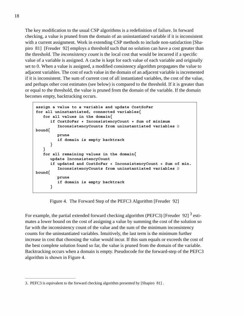
The key modification to the usual CSP algorithms is a redefinition of failure. In forwardchecking, a value is pruned from the domain of an uninstantiated variable if it is inconsistentwith a current assignment. Work in extending CSP methods to include non-satisfaction [Sha-piro 81] [Freuder 92] employs a threshold such that no solution can have a cost greater thanthe threshold. The inconsistency count is the local cost that would be incurred if a specificvalue of a variable is assigned. A cache is kept for each value of each variable and originallyset to 0. When a value is assigned, a modified consistency algorithm propagates the value toadjacent variables. The cost of each value in the domain of an adjacent variable is incrementedif it is inconsistent. The sum of current cost of all instantiated variables, the cost of the value,and perhaps other cost estimates (see below) is compared to the threshold. If it is greater thanor equal to the threshold, the value is pruned from the domain of the variable. If the domainbecomes empty, backtracking occurs.

Figure 4. The Forward Step of the PEFC3 Algorithm [Freuder 92]

For example, the partial extended forward checking algorithm (PEFC3) [Freuder 92] 3 esti-mates a lower bound on the cost of assigning a value by summing the cost of the solution sofar with the inconsistency count of the value and the sum of the minimum inconsistencycounts for the uninstantiated variables. Intuitively, the last term is the minimum furtherincrease in cost that choosing the value would incur. If this sum equals or exceeds the cost ofthe best complete solution found so far, the value is pruned from the domain of the variable.Backtracking occurs when a domain is empty. Pseudocode for the forward-step of the PEFC3algorithm is shown in Figure 4.

3. PEFC3 is equivalent to the forward checking algorithm presented by [Shapiro 81] .

assign a value to a variable and update CostSoFarfor all uninstantiated, connected variables{

for all values in the domain{if CostSoFar + InconsistencyCount + Sum of minimum

InconsistencyCounts from uninstantiated variables ≥bound{

pruneif domain is empty backtrack

}}for all remaining values in the domain{

update InconsistencyCountif updated and CostSoFar + InconsistencyCount + Sum of min.

InconsistencyCounts from uninstantiated variables ≥bound{

pruneif domain is empty backtrack

}

19

Four algorithms are proposed by [Shapiro 81] for use in machine vision object labeling: nor-mal backtracking, forward checking, lookahead by one, and lookahead by two. The algo-rithms use increasingly sophisticated mechanisms to estimate a lower bound on the cost of alabel. The general form is a tree-search bounded by the cost threshold as described above.User-defined compatibility costs are assigned to each possible label tuple. Experiments usingrandomly generated labeling problems and the first three algorithms show that the forwardchecking algorithm performed best.

A more systematic extension of CSP algorithms is due to [Freuder 89] [Freuder 92] . In thisPartial Constraint Satisfaction Problem (PCSP) work, each constraint incurs a cost of 1 if it isleft unsatisfied. The problems are defined so that a solution where all constraints are satisfieddoes not exist. The goal is to find the valuation that fails to satisfy as few constraints as possi-ble. Adaptations of simple backtracking, backjumping, backmarking, as well as arc consis-tency and a variety of forward checking techniques are developed. A large set of experimentsis performed comparing these algorithms on a variety of randomly generated PCSPs and on aset of difficult graph coloring problems. Results indicate that these algorithms perform well onthe wide variety of problems. PEFC3 was generally superior across all the problem types. Wepresent a comparison of our relaxation algorithms to the PEFC3 algorithm in Chapter 4.

PCSPs have been addressed with a distributed partial constraint satisfaction algorithm[Ghedira 94] . Each variable and each constraint is modeled as an agent with simple behav-iour. A variable chooses a value for itself, polls its constraints for satisfaction, and accepts orrejects the new state based on a simulated annealing approach. The asymptotic convergence ofthe algorithm is shown; however it is recognized that this convergence is impossible to obtainin practice. No experimental results are presented.

The GSAT algorithm [Selman 92] operates on a problem that is, at least superficially, similarto PCSPs. Given a set of propositional clauses with a random assignment of truth values, theGSAT procedure changes the truth value of the literal that leads to the largest increase in thetotal number of satisfied clauses. The flipping of truth values continues until a satisfying solu-tion is found or a bound on the number of flips is met. The GSAT method, which employs afull one-step lookahead, is surprisingly effective at finding solutions. The difficultly withextending GSAT to PCSPs (or general constraint problems) is the very small domain for eachvariable (i.e. {TRUE, FALSE}). It is not clear that the GSAT technique, which is expensive interms of the size of the possible successor states it investigates, can be extended to a broaderrange of problems.

2.4 Constraint Optimization

Constraint relaxation problems are properly a subset of constraint optimization problems.Constraint optimization attempts to optimize the value of a general function over the variablesin the problem while constraint relaxation is optimization the sum of the costs of the con-straints.

20

2.4.1 Optimization in Operations Research

Optimization has traditionally been the purview of Operations Research (OR) techniques,such as linear and integer programming. The mathematical programming techniques centeraround a matrix representation of the problem variables and problem solving consists of oper-ations on the matrix. There are some difficulties in the application of these methods to optimi-zation problems investigated in AI research.4 These problems include the following:

• Techniques such as integer programming show a tendency to be overwhelmed by the num-ber of variables and values needed to represent non-trivial problems [Van 89] [Fox 90][Sadeh 91] [Dorn 92] . Furthermore, these techniques often place restrictions on the con-straints and variables that are not justified by the problem definition.

• Mapping a problem into the OR representation often necessitates a substantial increase inthe number of variables and constraints used in other representations [Van 89] . This fur-ther aggravates the tendency for OR techniques to be overwhelmed by large problems.

• Mathematical programming approaches are awkward when a concrete measure of optimal-ity can not be formulated [Dorn 92] . Such situations can arise from complex and conflict-ing problem objectives.

• There is difficulty in dealing with uncertainty [Dorn 92] .• Specific problem features can not be exploited;5 nor can particular heuristics be used [Van

89] .

Sensitivity analysis is the sub-field of Operations Research concerned with modifications to aproblem definition after the problem has been solved. There are methods that, given an opti-mal solution, can assess the impact of changes to the problem constraints [Phillips 76] [Baz-araa 90] . These methods do not deal with overconstrained situations and, furthermore, do notprovide any methods to identify constraints that are critical to the infeasibility of the problem.

Sensitivity analysis, using the theory of duality, allows for the simple derivation of shadowprices once the original problem is solved [Hillier 80] [Ravindran 87] . In a scheduling prob-lem, the shadow price is the net impact on the total profit of additional unit of a particularresource. These increments are only valid within a range of resource quantities as the purchaseof more will change the identity of the optimal solution (calculated by the original ORmethod). We will return to shadow prices later, in the context of predicting the impact ofscheduling decisions. For now, note that while shadow prices are inexpensively derived fromthe calculation of an optimal solution with OR methods, the original calculation is subject tothe drawbacks discussed here. Additionally, the fact that the shadow prices are valid onlywithin a range limits the generality with which alternative resource purchases can be explored.

4. Despite these difficulties, there is a growing realization that benefits would accrue from the marriage of AIand OR techniques [Lowry 92] [Interrante 93] .

5. We assert that utilization of problem features identified with texture measures is a fundamental technique inheuristic problem solving.

21

The OR branch-and-bound methodology discussed in Chapter 1 (Section 1.2.2) uses solutionsto relaxed versions of the problem to bound search in the original. This is of little use when theoriginal problem is infeasible, since there is no easily available information about critical con-straints. Furthermore, it is typical that only certain types of constraints can be relaxed to find abound (e.g. relax the requirement that a subset of variables have integer values).

2.4.2 Optimization in Artificial Intelligence

[Dechter 90] presents an optimization algorithm based on transformations of the constraintgraph. The optimization function is defined as the sum of a number of sub-functions whereeach sub-function operates on a subset of the problem variables. The containment criteriarequires that the set of variables in each sub-function must be constrained by at least one prob-lem constraint. For example, we have a problem with variables x1, …, x5 and the objectivefunctions f(x1, …, x5) = f1(x1, x3) + f2(x2, x3, x4) + f3(x5). The containment criteria is met bythe constraints: c1(x1, x2, x3, x4) and c2(x2, x5): f1 and f2 are contained by c1 and f3 is con-tained by c2.

The constraint graph is transformed into a dual constraint graph, where each constraint is anode and arcs are labeled with the variables shared between the constraints. In special cases, ajoin-tree [Dechter 89] can be constructed where each node represents a cluster of related vari-ables and the children of a node contain a subset of the variables in the parent. It is shown that,if the containment criteria is met and a join-tree can be created, the optimal tuple for a nodecan be calculated by choosing the maximally-rated tuples from the children. Therefore, theoptimization is a recurrence algorithm beginning with the leaves and flowing toward the rootwith a complexity linear in the number of constraints and tuples.

When the objective function does not meet the containment criteria and the graph does nothave a join-tree, the constraint graph is augmented following a tree-clustering algorithm[Dechter 89] . The tree clustering adds constraints to the graph in order to establish the boththe containment condition and the necessary requirements for the dual graph to have a join-tree. The complexity of the overall algorithm is dominated by the need to solve a CSP at eachnode of the dual constraint graph.

[Yokoo 92a] address constraint optimization in a distributed environment where each agenthas one variable and is aware of all associated constraints. Each agent also has a local objec-tive function defined over all variables in the problem. A modified form of the distributedasynchronous backtracking algorithm [Yokoo 92b] is used where agents choose a local valueand notify adjacent agents according to an ordering of the agents. The modified algorithmallows each agent to employ its own cost threshold and discover when no solution is possibleat the current threshold. In that case, the agent increments its local threshold and continues thesearch. The discovery and incrementing is done independently by each agent.6

6. The optimization algorithm is similar to the weight-based algorithm noted in Section 2.2 [Yokoo 93] .

22

2.5 Scheduling

Scheduling problems are constrained optimization problems that may not have even a satisfic-ing solution [Fox 90a] [Fox 90b]. In cases where the schedule is overconstrained, we needrelaxation to address this problem. In this section we will review work done in optimizedscheduling and in scheduling in overconstrained situations.

In constructive scheduling, a schedule is formed by the sequential assignment of start timesand resources to activities. If a consistent assignment cannot be made for an activity, back-tracking is done. Repair-based scheduling, in contrast, begins with a schedule that breaks oneor more of the problem constraints. By reassigning activity start times and resources, thesearch tries to find a valid schedule. Fuzzy logic has been used as a method of dealing withuncertainty and infeasibility.

2.5.1 Constructive Scheduling

The MICRO-BOSS scheduler [Sadeh 91] [Sadeh 94] builds on previous work in ISIS [Fox87] and OPIS [Smith 89] [Fox 90b]. A key difficulty in production scheduling is dealing withbottleneck resources. These are resources which are required by a number of activities over aparticular time interval. Earlier work [Smith 89] [Fox 90b] observed that bottleneck resourcesappeared and disappeared during scheduling depending on the scheduling decisions and thetime interval under consideration. Because the bottlenecks have significant impact on thequality of the schedule, it is necessary to be able to detect and react to the emergence of newbottlenecks during the scheduling process. MICRO-BOSS takes an activity-centered perspec-tive, allowing the focus of attention to be quickly shifted as the importance of activitieschange. This “micro-opportunistic” approach allows the dynamic identification of bottleneckresources which constitute important trade-offs and critical activities on those resources. Onceidentified, the critical activities are the focus of attention and, when the trade-offs areresolved, the rest of the problem is easier to solve.

Micro-opportunistic scheduling is applied to both satisficing scheduling and optimized sched-uling. The latter employs a cost model based on tardiness and inventory costs. Identificationof critical activities is done by use of texture measurements on the constraint graph represen-tation of the scheduling problem. By aggregation of information about contention for aresource over some time interval, the activity most dependent on the resource for which thereis the most contention can be identified. Time and resource reservations are then made on thebasis of a related texture measure that estimates the cost incurred by the reservation. Empiricalevidence shows that MICRO-BOSS outperforms the best of 39 combinations of priority dis-patch rules and release policies [Sadeh 94] .

23

2.5.2 Repair-based Scheduling

Recently, scheduling systems have been built in the repair-based paradigm, where local heu-ristics are applied to improve the original inconsistent solution [Johnston 92] [Mcmahon 92] [Zweben 94] . This is of interest from a relaxation perspective because relaxation can beviewed as a repair-based process. An inconsistent solution implicitly performs constraintrelaxations: if we accept the solution, we must relax the inconsistent constraints. Normalrepair-based scheduling attempts to minimize the number of unsatisfied constraints by modi-fying values of the variables. A relaxation algorithm is an effort to modify both the constraintsand the value instantiation to find a lower cost solution.

The MinConflicts algorithm [Minton 92] is representative of the repair-based algorithms.MinConflicts quickly finds an inconsistent starting solution and then iteratively chooses a con-flicting task and re-schedules it to a time that will minimize the number of conflicts it has withother tasks. The partial lookahead procedure simply tries to schedule the chosen task at eachpossible time and evaluates the solution by counting the number of conflicts. The algorithmends when no conflicts are left or a bound on the number of iterations has been met.

Despite the incompleteness of the approach, very good results have been achieved with theo-retical problems such as N-queens7 [Minton 92] and real-world problems such as schedulingobservations for the Hubble Space Telescope [Johnston 92] .

2.5.3 Fuzzy Scheduling

An approach to both the constrained optimization nature of scheduling and uncertainty in theschedule modeling is using fuzzy logic.

[Dorn 92] applies relaxation based on fuzzy sets to a production process scheduling domainwhere a job places significant constraints on jobs that may precede or follow it. Fuzzy linguis-tic values are used to rank the importance of individual jobs and compatibility of every pair ofjobs. Scheduling focuses attention first on the more important jobs. Typically, some jobs cannot be scheduled without violating constraints and some adjacent jobs will have a low com-patibility. A constraint that should be improved is found and the associated jobs are removedor exchanged with other jobs. An evaluation function is defined based on the fuzzy values ofconstraints and the search is heuristically guided on the basis of the evaluation function.

[Dubois 93] uses the fuzzy constraint model for job shop scheduling. The interpretation offuzzy constraints can be preferences surrounding hard constraints or uncertainty in the envi-ronment. The release date and due date of orders, and the duration of tasks are modeled asfuzzy values. The precedence constraints are also modeled as fuzzy sets: a constraint can besatisfied to different degrees. Given these fuzzy sets, the authors define the global satisfactionlevel to be the smallest extent to which a solution satisfies a constraint. This introduces a total

7. Place N queens on an N-by-N chess board such that no queen can attack another.

24

ordering over potential solutions which is exploited in the solving paradigm. The search is aclassical branch-and-bound depth-first search, interwoven with a propagation mechanism toensure the consistency of the fuzzy temporal windows and a lookahead analysis on whichdecisions are based. The lookahead procedure is based on an estimate of the decrease in thesatisfaction if the best choice is not made. This measure (which is used as the value orderingheuristic) is used as the variable ordering heuristic because it also estimates the “criticity” ofthe conflicts.8 Early empirical results indicate that fuzzy constraints are more productive thancrisp analysis as the flexibility and/or uncertainty of the problem can be captured with littleincrease in complexity. Further, it is asserted that the framework handles partially inconsistentproblems and can be easily extended to deal with constraint priorities.

It is interesting to contrast this approach with the constraint representation used in the ISISscheduler [Fox 87] . ISIS represents preferences by having the constraints express theiracceptance or rejection of a solution on a 3-point scale. The required constraints define theadmissible solutions while the preference constraints form a total ordering over all admissiblesolutions. Just as in the work of [Dubois 93] , the ranking of solutions allows the search topreferentially extend some solutions over others based on the satisfaction of the constraints.The fuzzy logic based satisfaction calculation finds the smallest extent to which any constraintis satisfied. The authors note that this satisfaction measurement means that the high degree ofsatisfaction of one constraint cannot counterbalance the low degree of satisfaction of anotheras is seen in ISIS. In other words, the fuzzy scheduler would prefer a solution where all con-straints are satisfied at a medium level over a solution where some constraints are highly satis-fied and others only satisfied at a low level. ISIS, in contrast, prefers solutions where the“sum” of the satisfaction is higher. Unfortunately, the critical question of which of these pref-erences leads to better schedules remains open and is probably dependent upon problem spe-cific and problem domain specific factors.

2.5.4 Estimating the Impact of a Scheduling Decision

Many scheduling techniques (including those reviewed above) attempt to estimate the impactof assigning a particular start time to an activity. Because of the number of constraints amongactivities, the impact of a particular assignment is not fully known until all other activities areassigned and the entire schedule can be evaluated. This is not helpful when the goal is to cre-ate the schedule in the first place. What is desirable, then, is an inexpensive ranking of possi-ble start times for an activity by an estimation of the impact of each one on the overall cost (orfeasibility) of the schedule. This estimation can form the basis for a value ordering heuristic ateach activity. A variety of static value orderings are possible based on dispatch rules, such asalways trying the values from earliest to latest start time. However, work on dynamic estima-tions [Sadeh 91] , based on information gathered from the current partially constructed sched-ule, shows that improvements can be made over the dispatch rules.

8. The notions of criticity and reduction in satisfaction are similar to criticality of activities and cost increasesused in MICRO-BOSS [Sadeh 91] .

25

The MRP-STAR [Morton 86] planning module is a system designed for ManufacturingResource Planning (MRP) and, as such, estimates the cost of sequencing jobs through a num-ber of (aggregate) workcenters. The systems models costs with scheduling costs (costs of rawmaterial and costs of using a workcenter, less immediate revenues received) and tardinesscosts (one-time cost penalty, accruing cost penalty, lost revenue, and lost good-will). This totalcost of formulated and, in the analysis, the derivative is taken. This derivative indicates themarginal cost of increasing lateness of a job. The authors referred to these costs as shadowprices, leveraging off the similarity to the OR concept of shadow prices (see Section 2.4.1).9

Calculation of the dynamic, or “shadow” price of a set of jobs at any given time is done by aniterative calculation beginning with some reasonable sequencing rule and using the derivativeof the total cost. On the basis of the calculation, the jobs are resequenced and the iterative pro-cedure continues. The shadow prices take into account not only the costs within an order, butalso intra-order costs in estimating the impact of scheduling decisions. The authors note, how-ever, that this computation can be expensive, there is a need to recalculate periodically, andthe prices are somewhat unstable.

The GERRY scheduler [Zweben 92] [Zweben 94] , a repair-based system much like theMinConflicts algorithm, uses the number of conflicts that an activity will have if it is assignedto a particular start time as an estimation of the global impact. The intuition is that the numberof local conflicts is a good estimator for the number of global violations. The results ofGERRY demonstrates that the intuition holds in a number of typical scheduling problems.

The MICRO-BOSS scheduling system uses the propagation of marginal costs within an orderto estimate the cost incurred by an assignment. Efficient methods for identifying and updatingboth the best start times and the marginal cost factors for each activity are implemented. Thecalculated estimate is shown to be useful in scheduling, however two major trade-offs aremade to achieve efficient computation. First, the methods are based on the particular costmodel that is used in the experimental problems. A different cost model requires a new algo-rithm to identify the best possible reservations for an activity. Secondly, the estimate of cost isbased only on information within an order. No attempt is made to gather information about theimpact of an assignment from other orders. The other orders are potentially affected by anassignment via resource constraints and therefore represent untapped information.

A related technique for finding the impact of an assignment is the propagation of preferencesthrough a temporal constraint graph [Sadeh 89] . All activities begin with a local preferencecurve over the values in its domain. The propagation, from an identified “central” activity,aggregates a curve reflecting the global preference for each possible reservation of that activ-ity. The aggregation is done with a recursive algorithm resting on the original local preferencecurves. Propagation techniques are given for cyclic and acyclic temporal constraint graphs.Unfortunately, the complexity of the propagation scheme is very high and therefore the algo-

9. OR shadow prices reflect the impact on the total profit of an increase (or decrease) in one unit of resource, theMRP-STAR shadow prices reflect the impact on the total cost of changing the execution time of a job by onetime unit.

26

rithms are intractable for even medium sized problems. Furthermore, the propagation isexplicitly designed for temporal graphs and therefore is not easily applicable to gatheringinformation from other orders.10 We build on this work in the specification of techniques forthe propagation of costs over all types of constraints.

2.6 Discussion

The work reviewed here falls into two broad categories:

• General techniques in the CSP literature.• Specific techniques for areas such as scheduling and vision.

The general techniques typically address pieces of the relaxation problem but fail to representkey dynamic and semantic issues. The constraint optimization work, the PCSP work, and theselective non-satisfaction of constraints by static weights do not address the meaning of con-straint relaxation. These techniques can not express that the impact of constraint relaxationdepends highly on how the constraint is modified (e.g. what new value tuples are allowed). Ifconstraint relaxation is to be used as an operator in search, we must have a more fine-grainedcontrol than simply ignoring or not ignoring a particular constraint. Because of the lack ofsemantics, it is hard to integrate meaningful heuristic decision making into these techniques.Without some basis on which to make search-guiding decisions, these exponential techniquescan not be used on problems of a reasonable size.

We view the PCSP work as a special case of the general relaxation problem. If we define arelaxation problem such that all relaxation costs are identical it becomes a PCSP problem. InChapter 4, we will compare the a number of relaxation algorithms to the PEFC3 algorithm ona number of PCSP problems.

In contrast, the more domain-specific literature allows the close integration of heuristics andbegins to represent the meaning of constraint relaxation. The lookahead analysis done by thescheduling algorithms is designed to estimate the impact of a particular decision and in somecases (e.g. ISIS) the decision may concern how a constraint is to be relaxed. Only one of themethods for the estimation of the impact of a reservation can account for inter-order costs.The shadow price calculation [Morton 86] uses a iterative calculation to take into accountboth temporal and resource interactions. However, the authors note that the calculation can beexpensive, the prices can be unstable, and that it is necessary to re-calculate the prices period-ically. The other scheduling work, using a more explicit constraint model, does not address thepropagation of information through all types of constraint. In Chapter 5, in order to redress

10. The authors address propagation in a temporal constraint graph with explicit disjunctions (e.g. activity Amust occur before or after activity B). Resource constraints can be modeled with these constraints, however thecomplexity of propagation is even higher.

27

this non-generality, we propose techniques to estimate the impact of a activity reservation.This impact is expressed in terms of the minimum cost relaxations necessary if that valuewere to be put in place.

The repair-based scheduling algorithms embody the general concept of repair-based searcharound which it is possible to build a relaxation algorithm. In Chapter 4, we define a relax-ation algorithm for PCSPs based on the MinConflicts scheduling algorithm. We compare thisalgorithm to other relaxation algorithms on the PCSP problems.

2.7 Summary

We have reviewed the previous work in a number of areas concentrating on work done inextending CSP techniques [Freuder 92] and work in scheduling [Sadeh 91] [Sadeh 94][Minton 92] . We will revisit both of these areas in later chapters.

The previous work does not formulate a notion of constraint relaxation that is both expressiveand flexible enough to be used in general constraint satisfaction problems while at the sametime allowing the integration of heuristics to apply algorithms to specific problem domains.

We now present a propagation-based schema for constraint relaxation algorithms. Not onlyare constraints seen as a conduit for the transmission of information through the constraintgraph, but they are in themselves loci of knowledge and computation. The work on preferencepropagation, reviewed above [Sadeh 89] , can be seen as a basis for the propagation schemethat we propose.

28

29

Chapter 3 A Schema for ConstraintRelaxation

This chapter presents a general definition of constraint relaxation applicable across all con-straint types. We introduce an algorithm schema that provides a framework for relaxation-based algorithms and the integration of heuristic techniques. It is necessary to take a generalapproach in order to make contributions toward constraint-directed reasoning theory as wellas to ensure that our techniques will be applicable across a wide range of domains and to het-erogeneous constraint models. Given the complexity of constraint-based problem solving, werequire that domain specific heuristics can be easily integrated to the algorithmic schema.

We propose a general, propagation-centered schema for constraint relaxation. The constraintmodel is introduced and we elucidate the relaxation schema with an extended example. Amore formal treatment of the basic propagation mechanism is then given. Finally, we suggesttwo approaches to dealing with the complexity of the relaxation schema.

3.1 Foundational Concepts

3.1.1 Constraint Model

We define the constraint relaxation problem as consisting of the following:

• V - a set of n variables {x1, …, xn} whose values come respectively from the discrete, finitedomains D1, …, Dn.

• C - a set of m constraints {c1, …, cm}. Each constraint, ck:• is defined over a subset of variables, {xi, …, xj} ⊆ V• contains a predicate, Satisfied(xi, …, xj), which returns TRUE to indicate that the con-

straint is satisfied by the current variable instantiation and FALSE otherwise. Thepredicate is defined on the Cartesian product of the domains of the relevant variables.

• contains a function, GenerateRelaxation, which returns a set of constraints, ,that are relaxations of the constraint. The set of value tuples that satisfy a relaxation isa superset of that which satisfies the original constraint. Relaxing a constraint is equiv-alent to replacing it with one of its relaxations.

• contains a function, RelaxationCost(cp), indicating the local cost incurred if the con-straint is replaced by relaxation cp. All costs are non-negative and the cost for a con-straint to relax to itself is 0.

• ⊆ V the set of variables directly constrained by constraint ci.

RCck

Vci

30

• ⊆ C the set of constraints on variable vj.

A solution to a constraint relaxation problem is an assignment of a value to each variable(from its respective domain) such that all constraints or relaxations are satisfied and the totalcost of the constraint graph (the sum of the cost of each relaxation) is as small as possible. Asolution to the original problem, with no relaxation, has a cost of 0 and is considered optimal.1

The RelaxationCost at a constraint is well-defined but possibly expensive to calculate. Weassume that modeling includes specification of a RelaxationCost function at each constraint.

Our model is a generalization of the usual CSP model and as such it can be used for CSP prob-lem solving by ignoring the GenerateRelaxation and RelaxationCost functions. It also gener-alizes work done in areas related to constraint relaxation discussed in the previous chapter.

3.1.2 Search With Relaxation

In CSP search there is typically a single operator: the assignment of a value to a variable. Heu-ristic techniques are designed to limit the number of alternative values that must be explored.Backtracking occurs when it is found that a previous choice can not lead to a solution.

Relaxation-based search has two operators: the assignment of a value to a variable and therelaxation of a constraint. For any complete value assignment, we can always find a solutionby relaxing constraints so that they are satisfied. Since we want to find a low cost solution,both the value assignments and the relaxations are important.

A generate-and-test algorithm can be used for relaxation problems. All possible value combi-nations are generated and, for each, the relaxations to find a solution are made. We store thesolution and produce another valuation. If a subsequent valuation has a lower cost, the previ-ously stored solution is replaced. For relaxation search, generate-and-test is more expensivethan it is for CSP search because all possible value combinations must be produced.

3.2 Relaxation-Based Search

The proposed relaxation schema has two stages:

1. Value/control/cost propagation - a value is assigned and propagated through the graph.Control is then propagated to another node (constraint or variable) where further value andcontrol propagation may be done. The value and control propagation eventually terminateand cost information, found on the basis of the value and control propagation, is gathered,cached, and propagated back. No commitment is made to particular assignments or relax-ations.

1. In many cases there exists no optimal solution due to contradictory constraints.

Cvj

31

2. Relaxation propagation - if the cost returned by the first stage is deemed acceptable, thegraph configuration corresponding to that cost is put in place by propagation of relaxations.This propagation, depending on cost information cached in the first stage, makes commit-ments to specific variable instantiations and constraint relaxations.

In this section, we will define propagation and provide an extended example of a relaxationalgorithm executed on a small constraint graph.

3.2.1 Propagation

Traditionally, propagation has been the transmission of information between variables overconstraint links. We extend this definition by making a constraint a first-class object. We pro-pose that a constraint is not simply a conduit of information but rather a locus of processingduring the propagation procedure. The propagation is not simply via a constraint, rather infor-mation is transmitted from object to object, where the objects are variables and constraints.When propagation reaches an object, action is taken based on the received information.

We propose four types of propagation, as follows:

1. Value propagation - After a variable is assigned to a value (or after a constraint is relaxed),value propagation transmits the information effect to neighboring nodes. Typically, theeffect of value propagation on a variable will be to prune the domain of possible values,because the decision invalidates some of the domain values. Similarly, at a constraint thenumber of possible relaxations will be pruned. Using the graph coloring example fromChapter 1, the assignment of blue to a variable followed by value propagation over a non-relaxable constraint, would prune the value blue from the adjacent variable.

2. Control propagation - When processing has completed at a node, the control proceeds tosome neighboring node where further processing is done. Both the identity of the neighbor-ing node and the processing undertaken upon arrival is dependent upon heuristics specifiedwhen the schema is instantiated. Usually, the action taken at a variable is the assignment ofa value. At a constraint, the action is the selection of a constraint (a relaxation of the con-straint or the constraint itself) that “replaces” the original constraint. The action mayinclude value propagation or continuation of control propagation.

3. Cost propagation - Once the value/control propagation has terminated (see below for termi-nation criteria), we propagate the cost associated with the graph back toward the variablewhere control propagation began (the source variable). This cost is a result of the schedul-ing decisions (the assignments and relaxations) made during the value/control propagation,therefore the cost information will flow backward along the path that control propagationoriginally took.

4. Relaxation propagation - The cost propagation provides aggregate information about thecost of the solution that can be found given a particular assignment of the source variable.On the basis of specified criteria, we may decide that the cost of one of the solutions isacceptable. Therefore, we commit to the value of the source variable corresponding to thesolution. We perform a propagation that traces the original propagation in order to committo assignments and relaxations searched through in the value/control/cost propagation

32

stage. Relaxation propagation consists of value propagation to promulgate the effects of adecision, followed by control propagation. In this case however, the action at each nodewill be to commit to a value assignment or relaxation based on cached cost information andcommitments that have already been made.

Propagation is based on the connectivity of the constraint graph. Information from a variablecan only be directly transmitted to a constraint on that variable. Similarly, the propagationfrom a constraint can only directly proceed to a variable attached to the constraint.

With perfect knowledge, a propagation-based algorithm is linear in the number of variablesand constraints. At each variable the correct value is assigned and at each constraint the opti-mal relaxation is made. We do not have this knowledge, therefore it is necessary to try differ-ent values at a variable and different relaxations at a constraint. The set of values that wesearch over at a variable is called the candidate value set. The set of relaxations that weattempt at a constraint is the set of candidate constraints.

For the balance of this chapter, we refer to the value and control propagation as value propa-gation. This simplification is made because we assume (in this chapter) that the effects of adecision only flow directly to the node to which control flows. It is not the case that the effectsof an assignment flow to all neighboring nodes and then control flows to only one. Both theeffects of an assignment and control flow to one neighboring node. Therefore, value propaga-tion will include transmitting the information on an assignment and the control to a uniqueneighboring node. In Chapter 5, we relax this simplification and implement separate value andcontrol propagation.

3.2.2 An Extended Example

Assume we choose x1 as the starting point in the graph shown in Figure 5. At each variable,the candidate value set will contain all values that are consistent with previously made relax-ations. Similarly, at each constraint the candidate constraint set contains all constraints that areconsistent with previous value assignments.

Figure 5. A Simple Constraint Graph

The following is a trace of the search of the graph in Figure 5:

x1 x2 x3

c1 c2

Variable Domains: {D1, D2, D3} = {{1,2},{1,2},{1,2}}

c1: Domain = {(1,1),(1,2)}

Relaxationsrc1: {(1,1),(1,2),(2,1)}rc2: {(1,1),(1,2),(2,2)}

Cost13

c2: Domain = {(2,1),(2,2)}

Relaxationsrc3: {(2,1),(2,2),(1,2)}

Cost1

rc4: {(2,1),(2,2),(1,1)} 2

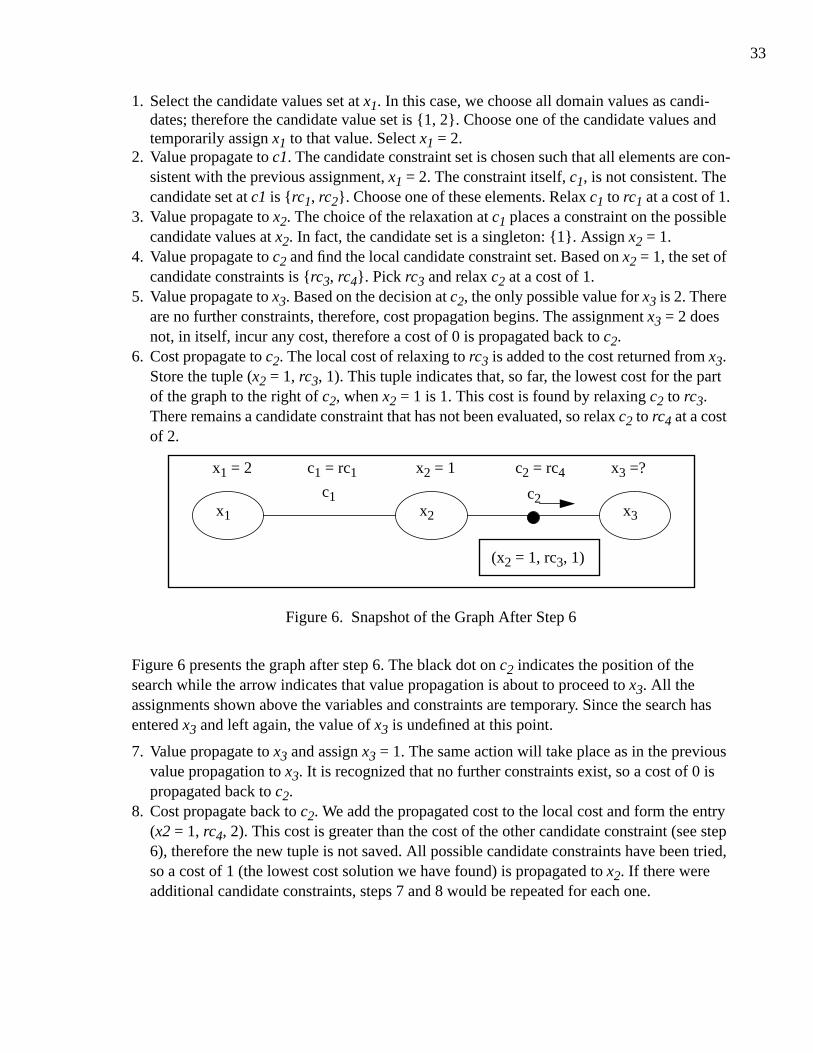
33

1. Select the candidate values set at x1. In this case, we choose all domain values as candi-dates; therefore the candidate value set is {1, 2}. Choose one of the candidate values andtemporarily assign x1 to that value. Select x1 = 2.

2. Value propagate to c1. The candidate constraint set is chosen such that all elements are con-sistent with the previous assignment, x1 = 2. The constraint itself, c1, is not consistent. Thecandidate set at c1 is {rc1, rc2}. Choose one of these elements. Relax c1 to rc1 at a cost of 1.

3. Value propagate to x2. The choice of the relaxation at c1 places a constraint on the possiblecandidate values at x2. In fact, the candidate set is a singleton: {1}. Assign x2 = 1.

4. Value propagate to c2 and find the local candidate constraint set. Based on x2 = 1, the set ofcandidate constraints is {rc3, rc4}. Pick rc3 and relax c2 at a cost of 1.

5. Value propagate to x3. Based on the decision at c2, the only possible value for x3 is 2. Thereare no further constraints, therefore, cost propagation begins. The assignment x3 = 2 doesnot, in itself, incur any cost, therefore a cost of 0 is propagated back to c2.

6. Cost propagate to c2. The local cost of relaxing to rc3 is added to the cost returned from x3.Store the tuple (x2 = 1, rc3, 1). This tuple indicates that, so far, the lowest cost for the partof the graph to the right of c2, when x2 = 1 is 1. This cost is found by relaxing c2 to rc3.There remains a candidate constraint that has not been evaluated, so relax c2 to rc4 at a costof 2.

Figure 6. Snapshot of the Graph After Step 6

Figure 6 presents the graph after step 6. The black dot on c2 indicates the position of thesearch while the arrow indicates that value propagation is about to proceed to x3. All theassignments shown above the variables and constraints are temporary. Since the search hasentered x3 and left again, the value of x3 is undefined at this point.

7. Value propagate to x3 and assign x3 = 1. The same action will take place as in the previousvalue propagation to x3. It is recognized that no further constraints exist, so a cost of 0 ispropagated back to c2.

8. Cost propagate back to c2. We add the propagated cost to the local cost and form the entry(x2 = 1, rc4, 2). This cost is greater than the cost of the other candidate constraint (see step6), therefore the new tuple is not saved. All possible candidate constraints have been tried,so a cost of 1 (the lowest cost solution we have found) is propagated to x2. If there wereadditional candidate constraints, steps 7 and 8 would be repeated for each one.

x1 x2 x3

c1 c2

x1 = 2 c1 = rc1 x2 = 1 x3 =?

(x2 = 1, rc3, 1)

c2 = rc4

34

9. Cost propagate to x2. Form the cost entry (x2 = 1, 1). Because there are no other cost entrieswith the index x2 = 1, this one is stored, indicating that it is the lowest cost solution we havefound. There are no other candidate values for x2 (see step 3, where the candidate value setwas created), therefore cost propagation continues.

10.Cost propagate to c1 and add the local relaxation cost to the propagated cost. Form andsave the cost entry: (x1 = 2, rc1, 2). This indicates that when x1 = 2, the lowest cost partialsolution we have found is 2. This cost corresponds to relaxing c1 to rc1. Not all candidateconstraints have been tried, so we relax c1 to rc2 at a cost of 3. Value propagation beginsagain to assess the cost of the subgraph with the new assignment.

11.Value propagate to x2. The relaxation rc2 constrains the value of x2 to be 2. This is the onlymember of the candidate value set, so assign it to x2.

12.Value propagate to c2. All local constraints are consistent with x2 = 2, therefore the candi-date constraint set is {c2, rc3, rc4}. Each of these constraints is assessed in turn just as wasdone above in steps 4 through 8. The ultimate local result is a cost entry (x2 = 2, c2, 0), indi-cating that when x2 = 2, the lowest cost solution to the subgraph is 0 and this occurs whenc2 is not relaxed. Propagate a cost of 0 back to x2.

13.Cost propagate to x2 and store (x2 = 2, 0). There are no more candidate values so cost prop-agation continues.

14.Cost propagate to c1. A cost of 0 is propagated back to c1 and this is added to the local costto form the entry (x1 = 2, rc2, 3). The cost of 3 is higher than the previous entry (x1 = 2, rc1,2) (see step 10) so the newer entry is discarded.

Figure 7. Snapshot of the Graph After Step 14

Figure 7 shows the search after step 14. Again the black dot indicates the current location ofthe search. The arrow indicates that cost propagation is about to proceed to x1. As with Figure6, when cost propagation leaves an object, the value (or relaxation) is undefined.

15.Cost propagate a cost of 2 to x1. Store the cost entry (x1 = 2, 2). There is another candidatevalue for x1. Temporarily assign x1 = 1 and value propagate to c1. Steps 1 through 14 arerepeated for the new value of x1.

x1 x2 x3

c1 c2

x1 = 2 c1 =? x2 =? x3 =?

(x2 = 1, rc3, 1)

c2 =?

(x2 = 2, c2, 0)(x2 = 1, 1)(x2 = 2, 0)

(x1 = 2, rc1, 2)

35

Figure 8. The Graph after All Value/Cost Propagation

Figure 8 displays the cost information that is gathered in the value/cost propagation phase.The information at x1 indicates that an assignment of x1 = 2 results in a solution of cost 2,while x1 = 1 leads to a zero-cost solution. The information stored at the other objects allowseither solution to be re-created. The actual modification of the graph occurs in the relaxationpropagation phase of the relaxation algorithm. The first step is to choose a value for the sourcevariable based on some criteria. Typically, we choose the value that leads to the minimum glo-bal cost solution. For the example, however, we choose x1 = 2 because it requires some relax-ation to be done.

The relaxation propagation takes the following steps (having chosen and assigned x1 = 2):

1. Propagate relaxation to c1. At c1, use the assignment x1 = 2 to find the correct relaxation inthe cache. It is the first entry shown in Figure 8: c1 is relaxed to rc1.

2. Propagate relaxation to x2. The relaxation rc1 requires x2 = 1. Assign this value. Had therelaxation of c1 allowed a number of assignments of x2, the lowest cost assignment fromthe cost cache would be chosen.

3. Propagate relaxation to c2. Locate the entry (x2 = 1, rc3, 1) which is the only entry with x2= 1. Relax c2 to rc3.

4. Propagate relaxation to x3. The relaxation of c2 to rc3 together with the assignment x2 = 1,requires x3 = 2. Assign this value.

The solution when x1 = 2 is shown in Figure 9.

Figure 9. The Graph of the Final Solution for x1 = 2

x1 x2 x3

c1 c2

x1 =? c1 =? x2 =? x3 =?

(x2 = 1, rc3, 1)

c2 =?

(x2 = 2, c2, 0)(x2 = 1, 1)(x2 = 2, 0)

(x1 = 2, rc1, 2)(x1 = 1, c1, 0)

(x1 = 2, 2)(x1 = 1, 0)

x1 x2 x3

c1 c2

x1 = 2 c1 = rc1 x2 = 1 x3 = 2c2 = rc3

36

3.2.3 Comments on the Example

There are a number of points that the extended example raises.

• The search is done in the value/cost propagation phase. The relaxation propagationdepends on the stored cost information.

• The lowest cost partial solution for each candidate value is stored in the cost cache at eachvariable. The cache is guaranteed to be no larger than the domain of the variable.

• There is an entry in the cost cache at each constraint for every candidate value of the previ-ous variable. This cache can be no larger than the domain of the previous variable.

• The information stored by the value/cost propagation is directional. The relaxation propa-gation must flow along each constraint in the same direction as the value propagation.

• If a variable has more than one constraint, the costs returned from each constraints aresummed. If x2 was the starting variable, the value propagation would proceed along c1 andc2 independently. The costs returned must be summed to form the cost entry at x2.

• All assignments made during value/cost propagation are temporary. This does not preventthe variable from already having a value. In a repair-based application, we can use the cur-rent value to aid in the selection of the candidate values and candidate constraints.

• If the size of the candidate constraint set at each constraint is k, and if p values are chosen ateach variable, then the complexity is O(pnkm), where m is the number of constraints and nis the number of variables reached in the propagation.

3.3 The Relaxation Schema

The relaxation schema is based on the propagation of information through the constraintgraph. The propagation is modulated by procedures that define the behaviour at five heuristicdecision points. Given the exponential complexity of the search, if a relaxation algorithm is tobe of practical use, we need to use heuristics to limit the selection of candidate values and con-straints. The decision points are the key places in the algorithm where heuristics can have sig-nificant impact on the solution quality vs. search effort trade-off. By selecting a small set ofalternatives from the possibilities, the complexity of the search will be reduced to a manage-able level, however the number of solutions investigated will be lessened. The selection ofsmall sets will result in a fast algorithm but a sub-optimal solution.2

The heuristic decision points are:

1. Selection of the source variable.2. Selection of a set of candidate values for each variable.3. Selection of a set of outgoing constraints from each variable.4. Selection of a set of candidate constraints at each outgoing constraint.

2. Despite the isolation of these decision points, there is no requirement to actually use heuristics in an instantia-tion of the schema. An algorithm can be defined which exhaustively searches through all the possibilities at eachdecision point.

37

5. Criteria for selection of a value-commitment at the source variable.

The source variable is the origin of the value propagation. Given the effects seen for differentvariable orderings in CSP solving, we expect this choice to have an impact on performance.

A set of candidate values are chosen for the source variable and for each variable that isentered by value propagation. It is not necessary that the same selection method be used forthe candidate value set at each variable.

The outgoing constraints are those along which propagation proceeds.3 At all variables exceptthe source variable, the selection is required to choose a subset of the constraints on the vari-able.4 The set of outgoing constraints defines the subgraph over which alternatives areassessed. As with candidate value selection, the same method need not be applied at everyvariable. Typically, selection of outgoing constraints will be based on the properties of theconstraint itself (e.g. its type or if it is relaxable) or on properties of subgraphs in which theconstraint participates (e.g. complete subgraphs).

Each candidate value is propagated along each outgoing constraint. Candidate constraints areselected at each outgoing constraint. A candidate constraint is either the constraint itself or arelaxation of the constraint produced by the GenerateRelaxation function.

After, the value/cost propagation has returned to the source variable, it is necessary to choosea value to assign to the source variable. This value-commitment is the beginning of the relax-ation propagation and will be based on the gathered cost information. Typically, the value cho-sen will be the one that leads to the lowest global cost, however it is not necessary to committo a value. Because the heuristic decision points specify that only a subset of possible solu-tions are searched over, it may be the case that the none of the solutions meet the criteria. Inthis case, no relaxation propagation is done, the gathered costs are discarded, and anothersource variable may be chosen. By making the value-commitment a heuristic decision point,we are allowing the integration of such techniques as simulated annealing [Kirkpatrick 83] ,where an new solution is entered based on a complex function of the its cost and the amountof processing already done.

The relaxation algorithm used in the example is specified as follows:

• Source variable: x1.• Candidate values: All values in the domain of the variable that are consistent with previous

choices.• Outgoing constraints: All constraints except the constraint from where the value propaga-

tion entered a variable. For example, c1 is not an outgoing constraint at x2 because valuepropagation visited c1 before reaching x2.

• Candidate constraints: All relaxations that are satisfied by the previous decisions.

3. Because we are combining value and control propagation, we specify a single set of outgoing constraints.More generally, there is a set of outgoing constraints for value propagation and a set for control propagation.

4. A constraint can only be an outgoing constraint for one variable.

38

• Value-commitment: Arbitrarily choose x1 = 2, as it requires relaxation of some constraints.

It is useful to re-iterate that the selection of the sets of candidate values, outgoing constraints,and candidate constraints limits the size of the graph and the size of the search on the sub-graph. If the heuristics are based on local data or data gathered from a subgraph (e.g. localrelaxation costs), the relaxation algorithm may be incomplete: it is not guaranteed to find theminimal cost solution. We see this as a classic trade-off between processing time and the qual-ity of solution. An area for future work is the characterization of the types of trade-offs madeby relaxation algorithms using different heuristics to limit the search (see Chapter 7).

3.4 Basic Propagation

With the intuition provided by the extended example, we now examine more formally thebasic propagation mechanisms upon which the schema is built. These propagation methodsbuild on work on preference propagation [Sadeh 89] .

3.4.1 Value and Cost Propagation

Before propagation can begin, a variable, xsource ∈ V, a set of candidate values for that vari-able, VALsource ⊆ Dsource, and a set of outgoing constraints, , must be selected.We will assume these tasks have already been done. For each value, vj ∈ VALsource, weattempt to answer the question: what is the minimum cost graph we can find with xsource = vj?To answer this question, we calculate the PostCost: vj is propagated along each outgoing con-straint and the costs that are returned are summed.

(1)

The ConCost function can be broken into two other functions.

(2)

Where:

ci is the constraint connecting xa and xb.

is the set of candidate constraints for constraint ci.

RelaxationCost(rck) is the RelaxationCost function of ci.

vp is a value (in the domain of xb) such that Satisfied(rck | vj, vp) is TRUE.

CONxsource

PostCost xsource vj=( ) ConCost ci xsource vj=( )ci CONxsource

∈∑=

ConCost ci xa vj=( ) =

minrck CCci∈ RelaxationCost rck( ) PostCostrck

xb vp=( )+( )

CCci

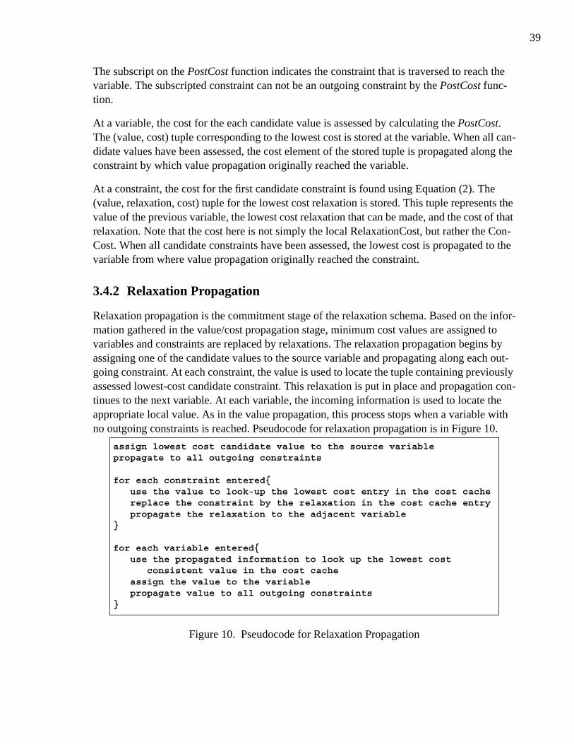
39

The subscript on the PostCost function indicates the constraint that is traversed to reach thevariable. The subscripted constraint can not be an outgoing constraint by the PostCost func-tion.

At a variable, the cost for the each candidate value is assessed by calculating the PostCost.The (value, cost) tuple corresponding to the lowest cost is stored at the variable. When all can-didate values have been assessed, the cost element of the stored tuple is propagated along theconstraint by which value propagation originally reached the variable.

At a constraint, the cost for the first candidate constraint is found using Equation (2). The(value, relaxation, cost) tuple for the lowest cost relaxation is stored. This tuple represents thevalue of the previous variable, the lowest cost relaxation that can be made, and the cost of thatrelaxation. Note that the cost here is not simply the local RelaxationCost, but rather the Con-Cost. When all candidate constraints have been assessed, the lowest cost is propagated to thevariable from where value propagation originally reached the constraint.

3.4.2 Relaxation Propagation

Relaxation propagation is the commitment stage of the relaxation schema. Based on the infor-mation gathered in the value/cost propagation stage, minimum cost values are assigned tovariables and constraints are replaced by relaxations. The relaxation propagation begins byassigning one of the candidate values to the source variable and propagating along each out-going constraint. At each constraint, the value is used to locate the tuple containing previouslyassessed lowest-cost candidate constraint. This relaxation is put in place and propagation con-tinues to the next variable. At each variable, the incoming information is used to locate theappropriate local value. As in the value propagation, this process stops when a variable withno outgoing constraints is reached. Pseudocode for relaxation propagation is in Figure 10.

Figure 10. Pseudocode for Relaxation Propagation

assign lowest cost candidate value to the source variablepropagate to all outgoing constraints

for each constraint entered{use the value to look-up the lowest cost entry in the cost cachereplace the constraint by the relaxation in the cost cache entrypropagate the relaxation to the adjacent variable

}

for each variable entered{use the propagated information to look up the lowest cost

consistent value in the cost cacheassign the value to the variablepropagate value to all outgoing constraints

}

40

No search is involved in relaxation propagation. The value that is propagated from a variableuniquely identifies the appropriate candidate constraint value. Each constraint is visitedexactly once during the relaxation propagation.

3.4.3 Termination of Propagation

It remains to be shown that propagation will terminate on any constraint graph. The cost andrelaxation propagation only retrace constraints and variables visited by value propagation.5

Therefore, it is sufficient to show that the value propagation will terminate.

First, note that the sets selected at each decision point are finite. The candidate value set isfinite because it is a subset of the domain of the variable and, by definition, the domain isfinite. The set of candidate variables at a constraint is a subset of all possible relaxations of theconstraint plus the constraint itself. A relaxation must be satisfied by at least one element inthe Cartesian product of the domains of the variables which it constrains. Therefore, the max-imum number of relaxations of a constraint is equal to the size of the power set of the Carte-sian product of the relevant variable domains. Since both the number of variables and the sizeof the variable domains is finite, the number of relaxations must also be finite. Finally, thetotal number of constraints in a graph is finite, therefore the constraints on one variable mustbe finite, and it follows that the set of outgoing constraints at a variable is finite.

Value propagation terminates when a variable selects an empty set of outgoing constraints. Wespecify that the set of outgoing constraints can not contain the constraint that was propagatedalong to reach the variable. In an acyclic graph, we are guaranteed to reach a variable that hasa single constraint. The single constraint is where that value propagation entered the variable,therefore the variable must select an empty set of outgoing constraints. In this case we definethe PostCost function at that variable to be equal to 0.

Given a cyclic graph, it is possible for value propagation to leave a variable and re-enter it viaanother constraint. To ensure termination, we expand the termination criteria for value propa-gation. In addition to stopping when a variable selects an empty set of outgoing constraints,value propagation must also stop when it re-enters a variable along a different constraint thanpreviously. To detect this occurrence, two registers are created at each variable. The first con-tains the AlreadyVisited flag that is set when a value is propagated to the variable and unsetwhen cost propagation leaves the variable. The second register, valready stores the currentlyassigned candidate value. If the variable is re-entered during value propagation, the cycle isdetected because the AlreadyVisited flag is already set. We redefine PostCost as in Figure 11.

5. Cost propagation traces the value propagation in the opposite direction.

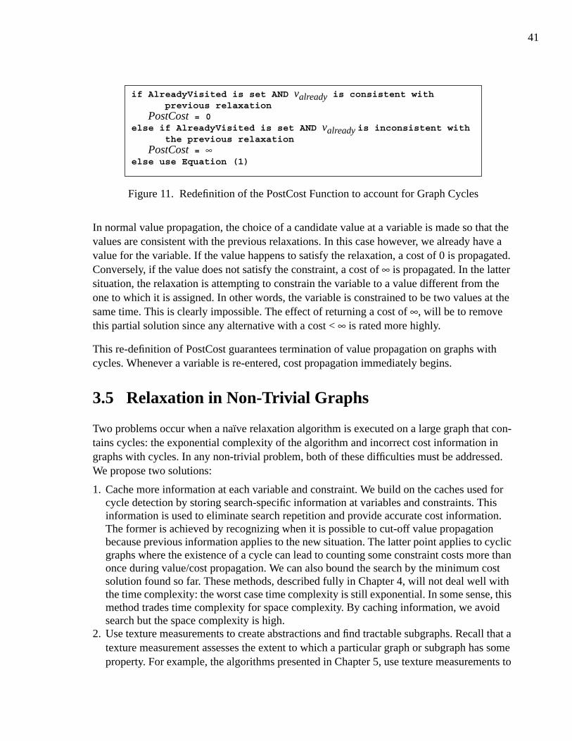
41

Figure 11. Redefinition of the PostCost Function to account for Graph Cycles

In normal value propagation, the choice of a candidate value at a variable is made so that thevalues are consistent with the previous relaxations. In this case however, we already have avalue for the variable. If the value happens to satisfy the relaxation, a cost of 0 is propagated.Conversely, if the value does not satisfy the constraint, a cost of ∞ is propagated. In the lattersituation, the relaxation is attempting to constrain the variable to a value different from theone to which it is assigned. In other words, the variable is constrained to be two values at thesame time. This is clearly impossible. The effect of returning a cost of ∞, will be to removethis partial solution since any alternative with a cost < ∞ is rated more highly.

This re-definition of PostCost guarantees termination of value propagation on graphs withcycles. Whenever a variable is re-entered, cost propagation immediately begins.

3.5 Relaxation in Non-Trivial Graphs

Two problems occur when a naïve relaxation algorithm is executed on a large graph that con-tains cycles: the exponential complexity of the algorithm and incorrect cost information ingraphs with cycles. In any non-trivial problem, both of these difficulties must be addressed.We propose two solutions:

1. Cache more information at each variable and constraint. We build on the caches used forcycle detection by storing search-specific information at variables and constraints. Thisinformation is used to eliminate search repetition and provide accurate cost information.The former is achieved by recognizing when it is possible to cut-off value propagationbecause previous information applies to the new situation. The latter point applies to cyclicgraphs where the existence of a cycle can lead to counting some constraint costs more thanonce during value/cost propagation. We can also bound the search by the minimum costsolution found so far. These methods, described fully in Chapter 4, will not deal well withthe time complexity: the worst case time complexity is still exponential. In some sense, thismethod trades time complexity for space complexity. By caching information, we avoidsearch but the space complexity is high.

2. Use texture measurements to create abstractions and find tractable subgraphs. Recall that atexture measurement assesses the extent to which a particular graph or subgraph has someproperty. For example, the algorithms presented in Chapter 5, use texture measurements to

if AlreadyVisited is set AND valready is consistent withprevious relaxation

PostCost = 0else if AlreadyVisited is set AND valready is inconsistent with

the previous relaxationPostCost = ∞

else use Equation (1)

42

identify a subgraph of tasks that form a good estimate of the global impact of schedulingdecisions. By the exploitation of the problem properties, the number of variables and con-straints over which propagation is done can be strictly limited. Relaxing different, smallsubgraphs (e.g. 5 to 8 variables) and choosing very few candidate values and candidateconstraints will minimize complexity difficulties. In dealing with graphs with cycles, thesubgraphs can be specifically chosen to be acyclic or techniques from the above approachcan be applied.

We view the second approach as more general and likely to result in usable algorithms. It con-centrates the relaxation algorithm on small subgraphs that are independent of the total graphsize. Despite the complexity difficulties with the first approach, these techniques are necessaryif the subgraphs found by texture measurements contain cycles. This approach is applicable tosmall problems (i.e. about 20 variables) such as Partial Constraint Satisfaction Problems(PCSPs) [Freuder 92] .

3.6 Summary

This chapter has presented a relaxation schema based on propagation of information throughconstraint graphs. It specifies five decision points that define the amount of propagation donein an instantiation of the schema. Given that the complexity of the search is exponential, wemust develop ways to efficiently identify good relaxations in non-trivial graphs. We sketchtwo approaches to this problem. The first utilizes caches of information at each variable andconstraint in order to identify cycles in the graph and eliminate repetition of search. The sec-ond uses texture measurements to identify important subgraphs and graph properties thatallow use of relaxation algorithms where the propagation is restricted.

In the following chapters we present algorithms defined using each of these approaches. InChapter 4, we examine the difficulties with cyclic graphs and employ information caches ateach variable and constraint to deal with these difficulties. Three repair-based algorithms forPCSPs are defined and their performance is compared with the PEFC3 algorithm. In Chapter5, we present a number of relaxation algorithms that use texture measurements to estimate theimpact of scheduling decisions in schedule optimization problems. We compare the estimatesto a baseline estimate found by Monte Carlo simulation.

43

Chapter 4 Cache-Based ConstraintRelaxation

This chapter investigates the use of information caches at each variable and constraint to min-imize search and ensure that the cost incurred by a cycle is correctly calculated. We definethree repair algorithms using the cache techniques and apply them to partial constraint satis-faction. We present an empirical evaluation of the performance of a number of variations ofthese three algorithms to PEFC3.

4.1 Difficulties With Cycles

When a graph contains cycles, an algorithm defined within the relaxation schema of the previ-ous chapter will encounter two difficulties:

1. The cost of a cyclic subgraph will be counted more than once.2. The information necessary for relaxation propagation may be corrupted.

We will examine each of these more closely and propose solutions.

4.1.1 Counting Cycle Costs

We use Figure 12 to demonstrate the first difficulty. Figure 13 shows a close-up of the propa-gation surrounding variable x1.

Value propagation enters x1 along c0. Constraints c1 and c2 are selected as outgoing con-straints and the propagation proceeds along c1 (Figure 13A). Value propagation will re-enterx1 via constraint c2. The cycle is detected and cost propagation immediately begins back alongc2 (Figure 13B). Cost propagation eventually returns to x1. An instantiation of the schema inthe previous chapter would then propagate the same candidate value along c2 and, when a costis returned, sum the two costs. The subgraph assessed by propagation along c1 is exactly thatassessed by propagation along c2. We count the cost of the subgraph twice.

44

Figure 12. A Constraint Graph with a Cycle

Figure 13. A Close-up of the Constraint Graph in Figure 12

Since the value propagation from x1 along c2 covers exactly the same constraints covered inthe previous propagation (along c1), we need not value propagate along c2. The next candidatevalue for x1 is selected or, if no candidate values remain, cost propagation continues backalong c0 (Figure 13C).

To detect when value propagation should not be done, we store additional information at eachvariable to identify co-cyclic constraints. As shown in Figure 13A, the identifier of the outgo-ing constraint is recorded: constraint c1 at variable x1. Upon re-entering a variable, we notethat the recorded constraint and the constraint that was returned on (c2 in this case) are co-cyclic. On returning the cost to x1, we know from the stored cycle information that we shouldnot follow the usual form of Equation 2 (see Chapter 3, Section 3.4.1). The set of outgoingconstraints is dynamically reconfigured by removing any constraint that takes part in a cycle.Our knowledge of co-cyclic constraints comes from re-entry into a variable after value propa-

x1

c1

c3 c4

c2

c0

x2 x3

x4

x1c1 c2

x1 = 4c0

Cost = 0

Cycle = (c1,c2)

vprop = 4

A

Value Propagation Cost Propagation

AlreadyVisited = 1valready = 4Outgoing = c1

B

Cost = C

C

Cost = C+ cost (c0)

Cycle = (c1,c2)

x1c1 c2

c0

x1c1 c2

c0

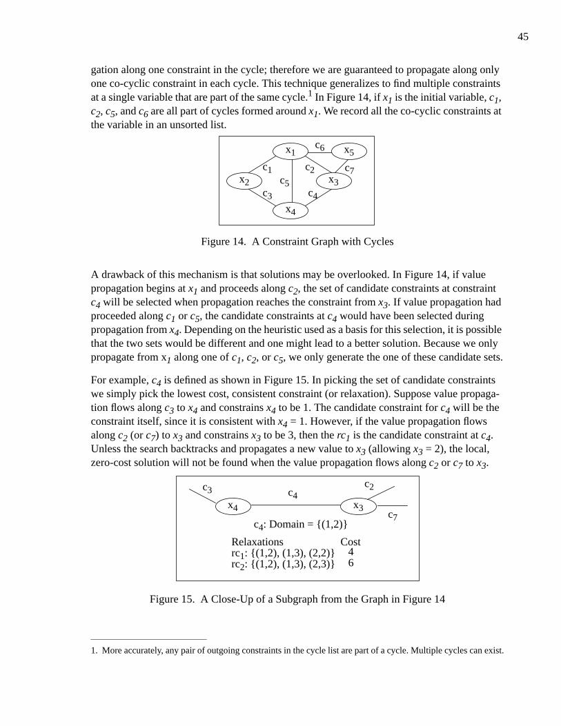
45

gation along one constraint in the cycle; therefore we are guaranteed to propagate along onlyone co-cyclic constraint in each cycle. This technique generalizes to find multiple constraintsat a single variable that are part of the same cycle.1 In Figure 14, if x1 is the initial variable, c1,c2, c5, and c6 are all part of cycles formed around x1. We record all the co-cyclic constraints atthe variable in an unsorted list.

Figure 14. A Constraint Graph with Cycles

A drawback of this mechanism is that solutions may be overlooked. In Figure 14, if valuepropagation begins at x1 and proceeds along c2, the set of candidate constraints at constraintc4 will be selected when propagation reaches the constraint from x3. If value propagation hadproceeded along c1 or c5, the candidate constraints at c4 would have been selected duringpropagation from x4. Depending on the heuristic used as a basis for this selection, it is possiblethat the two sets would be different and one might lead to a better solution. Because we onlypropagate from x1 along one of c1, c2, or c5, we only generate the one of these candidate sets.

For example, c4 is defined as shown in Figure 15. In picking the set of candidate constraintswe simply pick the lowest cost, consistent constraint (or relaxation). Suppose value propaga-tion flows along c3 to x4 and constrains x4 to be 1. The candidate constraint for c4 will be theconstraint itself, since it is consistent with x4 = 1. However, if the value propagation flowsalong c2 (or c7) to x3 and constrains x3 to be 3, then the rc1 is the candidate constraint at c4.Unless the search backtracks and propagates a new value to x3 (allowing x3 = 2), the local,zero-cost solution will not be found when the value propagation flows along c2 or c7 to x3.

Figure 15. A Close-Up of a Subgraph from the Graph in Figure 14

1. More accurately, any pair of outgoing constraints in the cycle list are part of a cycle. Multiple cycles can exist.

c1

c3 c4

c2c5

c6

c7

x4

x1 x5

x3x2

c4x4 x3

c4: Domain = {(1,2)}

Relaxationsrc1: {(1,2), (1,3), (2,2)}rc2: {(1,2), (1,3), (2,3)}

Cost46

c2c3

c7

46

Given that the algorithms within the schema will attempt to limit the number of alternativesthat are explored, the increase in complexity necessary to avoid this problem is not warranted.We accept that in relaxation on cyclic graphs, we may not be able to try all alternatives.

4.1.2 Relaxation Information

Relaxation propagation depends on the (value, relaxation, cost) tuple recorded at each con-straint. Recall that the value is a candidate value of the previous variable and that it is used asan index to the cost information during relaxation propagation. Because the value of the previ-ous variable is used as an index, relaxation propagation must enter a variable from the sameconstraint as in value propagation. If it does not, then the “previous” variable is not the samevariable as in value propagation, and the cost cache is meaningless.

We can ensure correct direction of relaxation propagation in a cyclic graph by modifying thecycle recording mechanism described above. Instead of using an unsorted list to store co-cyclic constraints, the outgoing constraint along which value propagation was done is the firstelement in the cycle list. Relaxation propagation can now identify the correct constraint totraverse. The other constraints in the list will be relaxed when they are reached later in therelaxation propagation.

A more serious problem concerns the cost cache at each constraint and variable. Recall thatthe cache at a constraint is indexed by a candidate value of the previous variable. The samevalue can be propagated to a variable more than once, resulting in the possibility that cacheelements may be overwritten. Without cycles, this is not a problem because the cost of a sub-tree is the same whenever an identical value is propagated to its root. When cycles areallowed, the “subtree” stemming from a variable, xb, can contain a variable, xa, that hasalready been given a value. When the next value is propagated to xb, the value of xa may havechanged (due to cost propagation back to xa and the choice of another candidate value). Thischanged value can have significant impact on the cost of the “subtree” at xb. If we index by thecandidate value of the previous variable, we will overwrite the cache with new, differententries. Relaxation propagation may require one of the older entries that no longer exists.

Figure 16A shows the value propagation entering the subgraph along c0 and proceeding alongc1. Eventually, the value propagation ends when x1 is re-entered from c3. Because the valuesx3 = 1, x1 = 1 are consistent with constraint c3, the entry (x3 = 1, c3, 0) is stored at c3. Costpropagation returns through x1 and eventually, due to a decision further back in the graph, avalue of x1 = 2 is propagated (Figure 16B). Again, value propagation continues until x1 is re-entered from c3. In this case, however, the constraint c3 must be relaxed to rc1 in order toallow the values x3 = 1, x1 = 2 to be consistent. Therefore, the cost cache entry (x3 = 1, rc1, 3)is stored at c3. Because the cost cache is indexed by the candidate value, the previous entry isoverwritten. The information on how to correctly relax c3, if x1 = 1 is assigned during relax-ation propagation, is no longer in the cost cache.

47

Figure 16. Overwriting the Cost Cache at a Constraint

A solution is achieved by attaching a context to the stored candidate constraint. The problemmanifests itself when a cycle causes the value propagation to return to a variable. When acycle is detected, we attach the (variable, valready) pair to the cost that is propagated back.This context is stored with the tuple at each constraint. The relaxation propagation mechanismnow not only uses the propagated value as an index, but also ensures that the stored contextmatches the current context. The match is found by checking that the stored value of eachvariable in the context corresponds to the value that the variable has been assigned.

In terms of the example in Figure 16, the original cost cache entry at c3 is now (x3 = 1, c3, 0,(x1, 1)). The subsequent cost cache entry is (x3 = 1, rc1, 3, (x1, 2)). The second entry does notoverwrite the first because the contexts are not equal. Relaxation propagation will therefore beable to locate the correct cost cache entry when it is making a commitment to a solution.

Since there can exist multiple cycles in the graph and many variables can appear “later” in thesearch tree, we must use a list of (variable, valready) pairs for the context. When the costreturned by each constraint to a variable is summed, the union of the attached contexts istaken. The summed cost and the united context are then propagated. No entries are removedfrom the context until a variable appearing in the context is reached in cost propagation. Atthat point, the variable removes its own (variable, valready) pair from the context list. The ele-ment can be deleted because all variables higher in the search tree were given a value beforethis variable, and therefore do not depend on the variable having a particular value.

x1

x3 x2

c1c2

c3

x1 = 1

x2 = 1x3 = 1

(x3 = 1, c3, 0)x1

x3 x2

c1c2

c3

x1 = 2

x2 = 1x3 = 1

c3: Domain: {(1,1)}Relaxationrc1: {(1,1), (1,2)}

Cost3

Value Propagation Cost Propagation

A B

c0 c0

(x3 = 1, rc1, 3)

(x3 = 1, rc1, 3)

48

4.1.3 Complexity

The two techniques above make use of caches at each variable and constraint. Lists of co-cyclic outgoing constraints are used to ensure proper cost counting of cycles. The total num-ber of all elements across all lists at a variable is limited to the number of constraints on thevariable. Each constraint only appears in one list because the lists represent independentcycles stemming from a variable. If a constraint were on more than one list, the cycles repre-sented by the two lists would not be independent.

Use of the context mechanism invalidates the space-complexity argument for the cost cachesgiven in the previous chapter. There we showed that the total size of the cache at a constraintwas limited to the number of candidate values at the previous variable. The context mecha-nism uses an entry at a constraint for each value of the previous variable and for each value ofthe variables in the context. Therefore, the space complexity for a cost cache at a single con-straint is O(Dk + 1), where D is the maximum domain size and k is the maximum number ofvariables that can be in a single context. The value of k will depend on the structure of thegraph. The worst case complexity occurs when the final variable to be visited in value propa-gation shares constraints with all other variables. The cache size at the constraint that was tra-versed to reach this final variable will have a cache size of O(Dn - 1), where n is the totalnumber of variables in the problem. Each constraint has a cost cache, therefore the complexityis further multiplied by the number of constraints.

Figure 17. A Graph Corresponding to the Worst-Case Space Complexity of the ContextMechanism

Figure 17 demonstrates the worst-case situation on a small graph. The constraints with arrowsrepresent the path that value propagation traveled to the final variable. The cost cache at the c*constraint will contain O(D4) entries.

4.2 Using Information Caches to Limit Search

We can use the cost caches at each variable and constraint to limit search by eliminating repe-tition and by cutting off the search when it is found that any solution to a subgraph will have alarger cost than a previously found solution.

c*

49

4.2.1 Using Stored Costs

In an acyclic graph, the minimum cost of a subtree with a particular value at the root will notchange when a new value is given to a variable higher up the tree. Significant time savings canbe achieved by storing the cost of the subtree for each candidate value of the root of the sub-tree. When value propagation returns to a variable (after cost propagation has left), the new setof candidate values is created. If this set contains elements also in previous candidate sets forthis variable, all that is necessary is a look-up of the previously calculated cost. Value propa-gation for a repeated value is unnecessary because all information stored in the subtree the lasttime the value was propagated is still valid.

When cycles exist, the caching mechanism must record the context. The argument used aboveto show the necessity of the context mechanism for relaxation propagation applies to caches atvariables. In order to cut off value propagation for a particular candidate value, we must findthe value in the cache and match the stored context with the current situation. By adding con-texts to the caches at each variable, we again increase the space complexity of the contextmechanism. Overall the worst-case space complexity of the caches at each constraint and vari-able is O(nmDn-1). Where n is the number of variables, m, the number of constraints, and D,the maximum domain size of any variable. This result strongly argues that the identification ofsubgraphs via texture measurements is necessary for practical application of these algorithms.

4.2.2 Bounding the Search

Work can be eliminated by ending part of the search when it is clear that any solution will nothave a cost lower than that the current best cost. We propagate the current lowest cost alongwith the value propagation and filter this bound at each variable and constraint.

Figure 18. Filtering the Cost Bound at a Variable

At a variable, for a particular candidate value we find the costs of all outgoing constraints. Ifwe have a bound on the cost of the subtree stemming from the variable, clearly the sum of thecosts returned from the outgoing constraints must be less than the bound if we are going toimprove the solution. Therefore, when one outgoing constraint returns its cost, we subtract the

current bound = bound passed to variablefor each candidate value{

for each outgoing constraint{get cost by propagation along outgoing constraint with

current boundcurrent bound -= costtotal cost += cost

}if total cost < current bound

current bound = total cost}

50

cost from the current bound. The resultant value is then used as the bound on the cost of thenext outgoing constraint. Similarly, if we find a new lowest cost solution with a particular can-didate value, that new cost becomes the bound on the solutions using the other candidate val-ues. Figure 18 shows the pseudocode for the filtering of the cost bound at a variable.

At a constraint, similar bound-filtering is done. When a candidate constraint is selected, itsRelaxationCost is subtracted from the bound. If the result is less than or equal to 0, any solu-tion using this candidate constraints will not improve on the current lowest cost solution.Therefore, we do not need to value propagate along that candidate constraint. If the result ofthe subtraction is greater than 0, we propagate it as the new bound. This is because the costfrom the subtree below the constraint must be less than the bound minus the cost of the con-straint. If the RelaxationCost of all candidate constraints is greater than the bound, a cost of -∞is returned to indicate a bound failure. The cost propagation mechanism checks for this flagand deals with it appropriately. Figure 19 presents the pseudocode for the filtering at a con-straint.

Figure 19. Filtering the Cost Bound at a Constraint

4.2.3 Enhancements

A number of additional enhancements are possible to the relaxation schema:

• Bounding the lookahead distance of the value propagation. The value propagation is com-plete in that it visits all variables connected via outgoing constraints. In larger graphs itmay be useful to be able to set a bound on the distance of the value propagation.

• Allowing the behaviour on cycle detection to be specified in the algorithm instantiation.• Providing a sufficient cost to the search. Whenever a complete solution is found that has a

cost that is equal to or less than the sufficient cost, search is stopped. In this way, thedesigner of the instantiation can specify when a solution is “good enough” to be acceptable.

current bound = bound passed to constraintfor each candidate constraint{

result = current bound - local costif result > 0{

get cost by propagation along candidate constraint withthe new bound = result

if cost + local cost < current boundcurrent bound = cost + local cost

}}

51

4.3 Cache-Based Relaxation Algorithms

We propose three incomplete (i.e. they are not guaranteed to find the minimal cost solutions)repair-based relaxation algorithms that use cost caching and search bounding mechanisms.General pseudocode is shown in Figure 20.

For each of the three relaxation algorithms:

• An initial solution is quickly found with a partial, non-backtracking (PNB) algorithm. Therelaxation algorithms are therefore repair-based since they try to iteratively improve theinitial solution.

• All domain values are used for the candidate values for the source variable.• The value propagated to an adjacent variable is the only candidate value for that variable.

This requires that a relaxation uniquely identify the value for the subsequent variable.2

Each candidate constraint is satisfied by a single tuple, thus the choice of candidate valuesis collapsed with the choice of the candidate constraints at the previous constraint.

• All attached constraints are selected as outgoing constraints. The only exception is the con-straint that is propagated along to reach the variable.

• The relaxation propagation is done only if the cost of a new solution is lower than the costof the current solution.

Figure 20. Pseudocode for the Main Loop of the Cache-Based Relaxation Algorithms

We embed instantiations of the relaxation schema within a loop based on the number of itera-tions. An iteration, therefore, is the selection of a source variable, value/cost propagation foreach value in the domain of the source variable, and relaxation propagation if a new, lowercost solution is found. The difference among the three algorithms is how the candidate con-straint set is chosen at each constraint. To fully specify each algorithm, we need only definehow we find an initial solution and the selection of candidate constraints.

2. In general, the candidate values at a variable need only satisfy the relaxations made to previous constraints.

find initial solution with PNB algorithmwhile(number of iterations ≤ iteration bound){

choose source variablefor each value in the domain of the variable{

temporarily assign the valuefind PostCost by propagating along all constraints

}if (lowest cost < current cost){

assign value corresponding to lowest costdo relaxation propagation

}number of iterations++

}

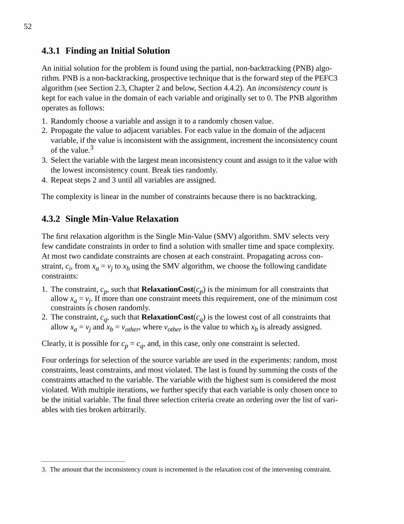
52

4.3.1 Finding an Initial Solution

An initial solution for the problem is found using the partial, non-backtracking (PNB) algo-rithm. PNB is a non-backtracking, prospective technique that is the forward step of the PEFC3algorithm (see Section 2.3, Chapter 2 and below, Section 4.4.2). An inconsistency count iskept for each value in the domain of each variable and originally set to 0. The PNB algorithmoperates as follows:

1. Randomly choose a variable and assign it to a randomly chosen value.2. Propagate the value to adjacent variables. For each value in the domain of the adjacent

variable, if the value is inconsistent with the assignment, increment the inconsistency countof the value.3

3. Select the variable with the largest mean inconsistency count and assign to it the value withthe lowest inconsistency count. Break ties randomly.

4. Repeat steps 2 and 3 until all variables are assigned.

The complexity is linear in the number of constraints because there is no backtracking.

4.3.2 Single Min-Value Relaxation

The first relaxation algorithm is the Single Min-Value (SMV) algorithm. SMV selects veryfew candidate constraints in order to find a solution with smaller time and space complexity.At most two candidate constraints are chosen at each constraint. Propagating across con-straint, ci, from xa = vj to xb using the SMV algorithm, we choose the following candidateconstraints:

1. The constraint, cp, such that RelaxationCost(cp) is the minimum for all constraints thatallow xa = vj. If more than one constraint meets this requirement, one of the minimum costconstraints is chosen randomly.

2. The constraint, cq, such that RelaxationCost(cq) is the lowest cost of all constraints thatallow xa = vj and xb = vother, where vother is the value to which xb is already assigned.

Clearly, it is possible for cp = cq, and, in this case, only one constraint is selected.

Four orderings for selection of the source variable are used in the experiments: random, mostconstraints, least constraints, and most violated. The last is found by summing the costs of theconstraints attached to the variable. The variable with the highest sum is considered the mostviolated. With multiple iterations, we further specify that each variable is only chosen once tobe the initial variable. The final three selection criteria create an ordering over the list of vari-ables with ties broken arbitrarily.

3. The amount that the inconsistency count is incremented is the relaxation cost of the intervening constraint.

53

Two termination criteria were used: 5 iterations and 10 iterations. Recall that in one iteration,a source variable is chosen, value/cost propagation is done with each of the values in thedomain of the source variable, and relaxation propagation is done if a new, lower cost solutionis found.

These options produce eight related algorithms.

4.3.3 Multiple Min-Value Relaxation

The Multiple Min-Value (MMV) algorithm is designed to find the cost of a larger number ofalternative graph configurations. It is therefore expected to find lower cost solutions thanSMV, but to use more effort in finding those solutions. The candidate constraints chosen are:

1. All constraints that allow xa = vj and minimize the local cost. As noted above, it is possiblefor a number of candidate constraints to have the same local cost while allowing xa = vj.

2. The constraint, cq, such that RelaxationCost(cq) is the lowest cost of all constraints thatallow xa = vj and xb = vother, where vother is the value to which xb is already assigned.

Only one constraint is selected if cq is the unique minimum cost constraint allowing xa = vj.

We use the same ordering for source variable selection as used in SMV and two options fortermination criteria: 1 iteration and 2 iterations. These termination criteria were used becausethe complexity of the MMV algorithm (see below) makes more iterations impractical.

Eight algorithms are specified.

a. The HL indicates the order is from High-to-Low number of con-straints. Similarly, LH indicates Low-to-High.

Variable Selection

Iterations

5 10

Random SMVR5 SMVR10

Most Constraints SMVHL5a SMVHL10

Least Constraints SMVLH5 SMVLH10

Most Violated SMVV5 SMVV10

TABLE 1. Variations of the SMV algorithm

Variable Selection

Iterations

1 2

Random MMVR1 MMVR2

Most Constraints MMVHL1 MMVHL2

Least Constraints MMVLH1 MMVLH2

Most Violated MMVV1 MMVV2

TABLE 2. Variations of the MMV algorithm

54

4.3.4 MinConflicts-like Relaxation

The MinConflicts repair algorithm chooses a variable with violated constraints, tries instanti-ating it to all possible values, and, if a lower cost configuration is found, assigns the minimumcost value to the variable. We define a MinConflicts-like (MC) algorithm in our schema. Thecandidate constraint chosen is:

1. The constraint, cq, such that RelaxationCost(cq) is the lowest cost of all constraints thatallow xa = vj and xb = vother, where vother is the value to which xb is already assigned.

The variable ordering for the source variable is the same as in MinConflicts: most violated.

There are two termination criteria: 20 iterations and 50 iterations. Because the only candidateconstraint is the one that makes the current assignments valid, the source variable is the onlyvariable whose value can change in a single iteration. If all variables are used as source vari-ables (in a series of iterations) and no relaxation has been done, then further iterations will notchange the solution. The search has found a state where it is required to change the value oftwo variables in a single iteration to find a lower cost solution. The MC algorithm can notmove from this state. We terminate the search when we detect this situation regardless of thenumber of iterations that have been completed.

These elements specify two algorithms.

The difference between MC and MinConflicts is the propagation. In the usual implementationof MinConflicts, there is no need to follow constraints through the graph since the cost onlychanges around the variable that is being moved. MC does more work than MinConflictsbecause it must traverse the entire graph and re-assign to each constraint the candidate con-straint to which it is already assigned. This has no effect on the cost of the graphs that MC willproduce relative to MinConflicts; however the effort expended in MC will be higher.

4.3.5 Complexity

Both SMV and MMV algorithms have a worst-case time complexity that is exponential in thenumber of constraints in the problem. The SMV complexity is O(D2m), where the maximumsize of the candidate constraint set is 2, D is the size of the domain for the initial variable, andm is the number of constraints. The complexity of the MMV algorithm is O(D( )m),where CCk is the set of candidate constraints at constraint, ck, and is the size of thelargest set of candidate constraints chosen for any outgoing constraint.

Variable Selection

Iterations

20 50

Most Violated MC20 MC50

TABLE 3. Variations of the MC algorithm

max CCk( )max CCk( )

55

The complexity of the MC algorithm is linear in D and the number of constraints. Only onecandidate constraint is chosen at each constraint; therefore, the each constraint is only tra-versed once. Cost propagation and relaxation propagation each traverse each constraint once.

4.4 Experiments with PCSPs

We have described the use of information caches to deal with cyclic graphs and decrease thetime complexity of the relaxation schema. These techniques show a high space complexityand, in some sense, achieve the improvement in time complexity only by creating space com-plexity difficulties. We expect that the algorithms defined here will be appropriate only onsmall problems where the space complexity is manageable. The Partial Constraint SatisfactionProblems (PCSPs) discussed in Chapter 2 are such problems. We now compare performanceof the above algorithms to the PEFC3 algorithm on a series of PCSPs.

4.4.1 Partial Constraint Satisfaction Revisited

A partial constraint satisfaction problem is an extension to CSPs [Freuder 92] . The problemsare defined so that a CSP solution (where all constraints are satisfied) does not exist due tocontradictory constraints. The goal is to find the valuation that fails to satisfy as few con-straints as possible. More formally, a PCSP is the following:

Given:

• A set, V, of n variables, {x1, …, xn}, each with a discrete, finite domain {D1,…, Dn}.• A set, C, of m binary constraints {c1, …, cm} each defined on a pair of the variables in V.

Find:

• An assignment of values to variables (from their respective domains) such that the maxi-mum number of constraints are satisfied.

In modeling PCSPs as a relaxation problem, we define that each constraint, ci, on variables xj,xk, has a compatibility set, CSi, of the form {(xj1, xk1), (xj2, xk2), …, (xjp, xkp)}. The compati-bility set specifies the pairs of values that satisfy the constraint. Constraint checking searchesthe compatibility set for the value-pair to which the variables are instantiated.

4.4.2 Partial Extended Forward Checking

In forward checking for CSPs, when a variable is instantiated the values of adjacent variablesthat are inconsistent with the instantiation are pruned. [Freuder 92] adapts forward checkingto PCSPs by keeping an inconsistency count for each value in the domain of each variable.The inconsistency count represents the cost of assigning the value to that variable. Originally,all inconsistency counts are 0. When a variable is instantiated, any value in the domain ofadjacent variables that is inconsistent has its inconsistency count incremented.

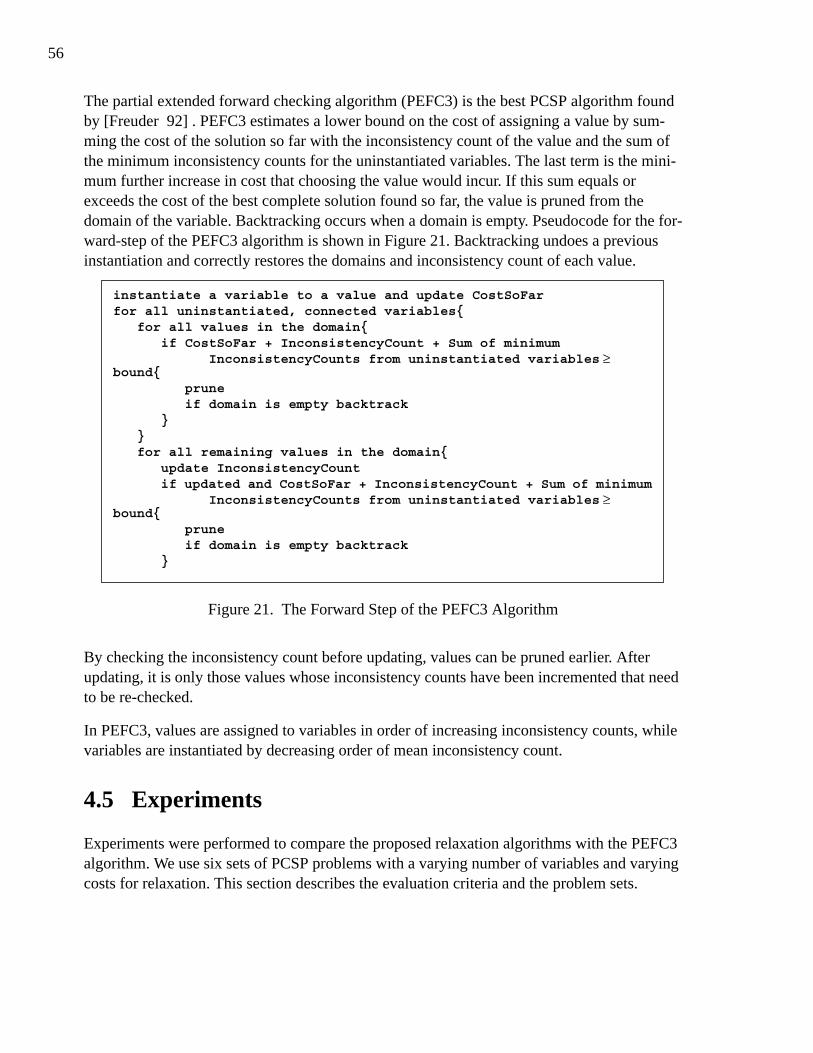
56

The partial extended forward checking algorithm (PEFC3) is the best PCSP algorithm foundby [Freuder 92] . PEFC3 estimates a lower bound on the cost of assigning a value by sum-ming the cost of the solution so far with the inconsistency count of the value and the sum ofthe minimum inconsistency counts for the uninstantiated variables. The last term is the mini-mum further increase in cost that choosing the value would incur. If this sum equals orexceeds the cost of the best complete solution found so far, the value is pruned from thedomain of the variable. Backtracking occurs when a domain is empty. Pseudocode for the for-ward-step of the PEFC3 algorithm is shown in Figure 21. Backtracking undoes a previousinstantiation and correctly restores the domains and inconsistency count of each value.

Figure 21. The Forward Step of the PEFC3 Algorithm

By checking the inconsistency count before updating, values can be pruned earlier. Afterupdating, it is only those values whose inconsistency counts have been incremented that needto be re-checked.

In PEFC3, values are assigned to variables in order of increasing inconsistency counts, whilevariables are instantiated by decreasing order of mean inconsistency count.

4.5 Experiments

Experiments were performed to compare the proposed relaxation algorithms with the PEFC3algorithm. We use six sets of PCSP problems with a varying number of variables and varyingcosts for relaxation. This section describes the evaluation criteria and the problem sets.

instantiate a variable to a value and update CostSoFarfor all uninstantiated, connected variables{

for all values in the domain{if CostSoFar + InconsistencyCount + Sum of minimum

InconsistencyCounts from uninstantiated variables ≥bound{

pruneif domain is empty backtrack

}}for all remaining values in the domain{

update InconsistencyCountif updated and CostSoFar + InconsistencyCount + Sum of minimum

InconsistencyCounts from uninstantiated variables ≥bound{

pruneif domain is empty backtrack

}

57

4.5.1 Evaluation Criteria

[Freuder 92] evaluates the algorithms by the number of consistency checks necessary to finda solution. In our model, we count the number of times the local cost of a value pair isaccessed. This is an exact analogue of the consistency checking. Where a consistency checkhas to access the constraint definition to find if a particular tuple satisfies the constraint, find-ing the local cost requires accessing the constraint definition to find the cost incurred at theconstraint by a tuple. Because of the format of the algorithms we propose, the local cost of apair is looked-up whenever one member of the pair is propagated across the constraint. There-fore, we are counting the number of times value propagation is done across any constraint.

The PNB algorithm, used to find an initial solution, and the relaxation propagation bothrequire a single access for each constraint in the graph. These counts are added to that fromthe relaxation algorithm to produce the results. In the presentation of our results we will, like[Freuder 92] , refer to this measure as the number of consistency checks. All of the relaxationalgorithms proposed here are not guaranteed to find the minimal cost solution, therefore wealso assess the cost of the solutions that are found.

In all algorithms where a random choice is made (all SMV algorithms, MMVR1, andMMVR2) the results presented are the average from five runs using different random seeds.

4.5.2 Problem Description

Six sets of PCSP problems were used for the experiments. Problem Sets 1, 3, and 5 were ran-domly generated by [Freuder 92] . Problem Sets 2, 4, and 6 were created from 1, 3, and 5respectively by giving a random cost in the range [1,9] to each value-pair not in the originalsatisfiability set.

[Freuder 92] creates many PCSP problems by varying four parameters: number of variables,number of constraints, domain size, and number of value-pairs in the compatibility set. Thefinal three parameters are represented by probability values which are held constant in theexperiments used here. The problem parameters are shown in Table 4.

ProblemSet

Number ofVariables

ExpectedDensity

ExpectedDomain

Size Satisfiability Costs

1 10 0.3 0.2 0.4 0-1

2 10 0.3 0.2 0.4 0-9

3 12 0.3 0.2 0.4 0-1

4 12 0.3 0.2 0.4 0-9

5 16 0.3 0.2 0.4 0-1

6 16 0.3 0.2 0.4 0-9

TABLE 4. Parameters of the Experimental Problems

58

In brief, the problems are constructed as follows:

• The number of variables is set and a spanning tree is created to ensure that all problems willcontain a single, connected graph.

• The expected density is used to determine the number of constraints added to the spanningtree. A value of 0.3 indicates that 30% of the possible constraints are added to the spanningtree graph.

• Expected domain size is based on a maximum domain size of twice the number of vari-ables. A value of 0.2 means that on average each domain has a size that is 40% of the num-ber of variables (2 × 0.2 × n).

• Finally, satisfiability indicates the proportion of the tuples in the cross-product of thedomains of adjacent variables that appear in the compatibility set of the connecting con-straint. A satisfiability value of 0.4 indicates that approximately 40% of the possible value-pairs satisfy the constraint connecting the variables.

Each of last two factors is applied separately to each domain or constraint. None of the prob-lems have a satisfying (i.e. zero cost) solution.

4.6 Results

Because we have 18 variations of relaxation algorithm, rather than comparing each to PEFC3,we first conduct preliminary experiments to compare the variations amongst themselves. Thevariations with the best results are then compared against PEFC3 on a larger set of problems.

4.6.1 Preliminary Experiments

The preliminary experiments used Problem Sets 1 and 3 to determine the best combination ofoptions for the relaxation algorithms. We focus on the cost results for two reasons. First, themain weakness of the relaxation algorithms, vis-a-vis the PEFC3 algorithm, is incomplete-ness. If the algorithm does not find a near-optimal solution, then it is not reliable enough foruse regardless of the reduction of effort. Secondly, the incomplete algorithms do significantlyless work than the PCSP algorithm in almost all cases.

In both the SMV and MMV algorithms, there was little systematic difference among the vari-ations. We were prevented from assessing the full effect of the manipulations in the termina-tion criteria because, in a large number of problems, the algorithm with the lower iterationbound found an optimal solution. It was observed that the SMVLH algorithms often found asolution of equal or lesser cost than any others and, in problems where improvements could berealized by further iterations, the largest cost decreases were seen with SMVLH. For thesereasons SMVLH5 and SMVLH10 are compared with PEFC3 below.

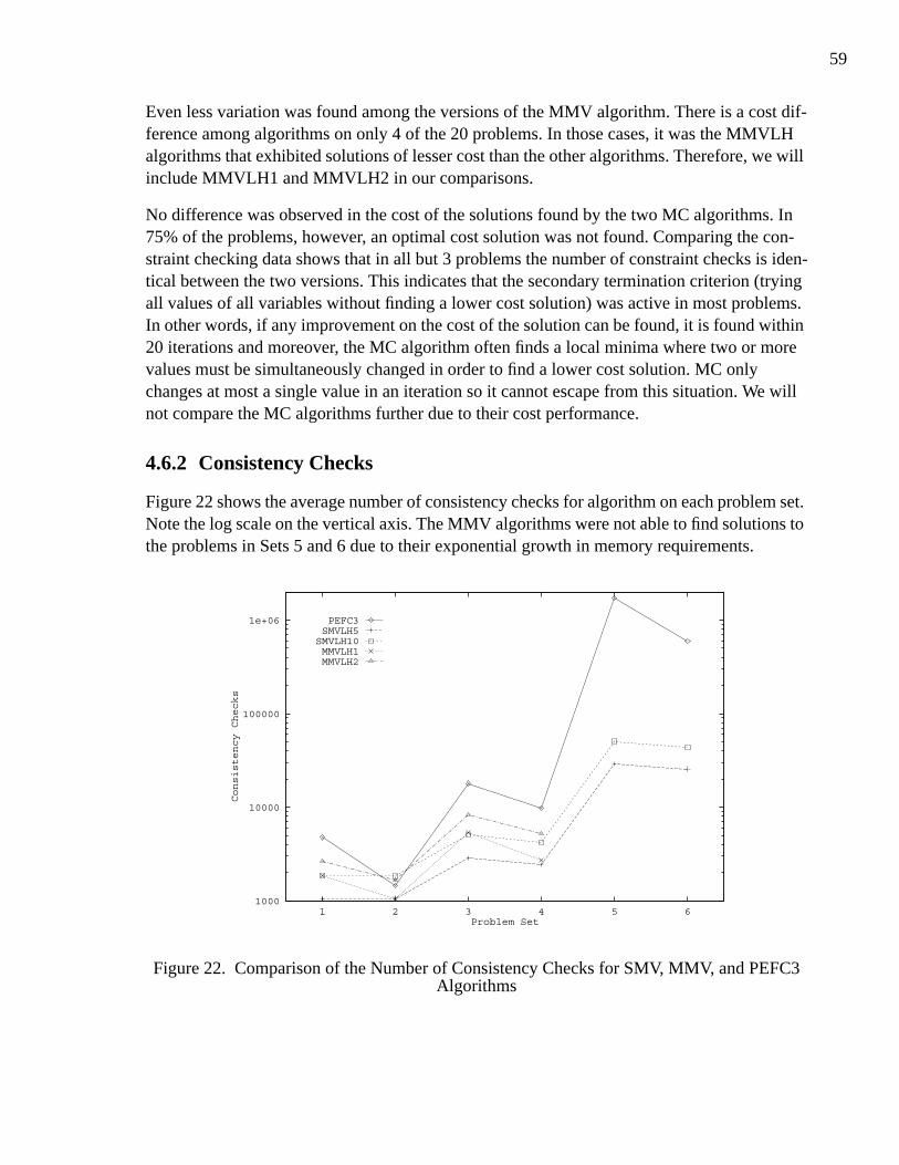
59

Even less variation was found among the versions of the MMV algorithm. There is a cost dif-ference among algorithms on only 4 of the 20 problems. In those cases, it was the MMVLHalgorithms that exhibited solutions of lesser cost than the other algorithms. Therefore, we willinclude MMVLH1 and MMVLH2 in our comparisons.

No difference was observed in the cost of the solutions found by the two MC algorithms. In75% of the problems, however, an optimal cost solution was not found. Comparing the con-straint checking data shows that in all but 3 problems the number of constraint checks is iden-tical between the two versions. This indicates that the secondary termination criterion (tryingall values of all variables without finding a lower cost solution) was active in most problems.In other words, if any improvement on the cost of the solution can be found, it is found within20 iterations and moreover, the MC algorithm often finds a local minima where two or morevalues must be simultaneously changed in order to find a lower cost solution. MC onlychanges at most a single value in an iteration so it cannot escape from this situation. We willnot compare the MC algorithms further due to their cost performance.

4.6.2 Consistency Checks

Figure 22 shows the average number of consistency checks for algorithm on each problem set.Note the log scale on the vertical axis. The MMV algorithms were not able to find solutions tothe problems in Sets 5 and 6 due to their exponential growth in memory requirements.

Figure 22. Comparison of the Number of Consistency Checks for SMV, MMV, and PEFC3Algorithms

1000

10000

100000

1e+06

1 2 3 4 5 6

Consistency Checks

Problem Set

PEFC3SMVLH5

SMVLH10MMVLH1MMVLH2

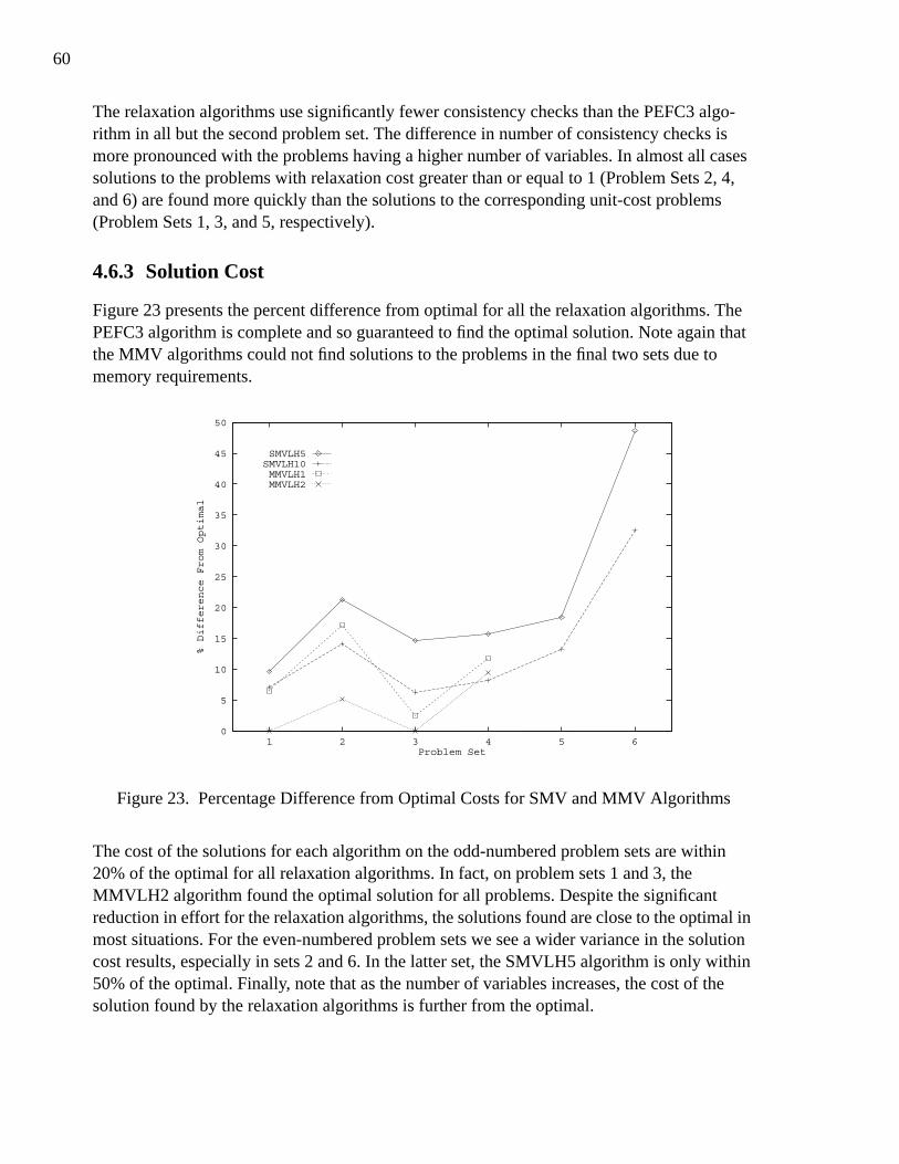
60

The relaxation algorithms use significantly fewer consistency checks than the PEFC3 algo-rithm in all but the second problem set. The difference in number of consistency checks ismore pronounced with the problems having a higher number of variables. In almost all casessolutions to the problems with relaxation cost greater than or equal to 1 (Problem Sets 2, 4,and 6) are found more quickly than the solutions to the corresponding unit-cost problems(Problem Sets 1, 3, and 5, respectively).

4.6.3 Solution Cost

Figure 23 presents the percent difference from optimal for all the relaxation algorithms. ThePEFC3 algorithm is complete and so guaranteed to find the optimal solution. Note again thatthe MMV algorithms could not find solutions to the problems in the final two sets due tomemory requirements.

Figure 23. Percentage Difference from Optimal Costs for SMV and MMV Algorithms

The cost of the solutions for each algorithm on the odd-numbered problem sets are within20% of the optimal for all relaxation algorithms. In fact, on problem sets 1 and 3, theMMVLH2 algorithm found the optimal solution for all problems. Despite the significantreduction in effort for the relaxation algorithms, the solutions found are close to the optimal inmost situations. For the even-numbered problem sets we see a wider variance in the solutioncost results, especially in sets 2 and 6. In the latter set, the SMVLH5 algorithm is only within50% of the optimal. Finally, note that as the number of variables increases, the cost of thesolution found by the relaxation algorithms is further from the optimal.

0

5

10

15

20

25

30

35

40

45

50

1 2 3 4 5 6

% Difference From Optimal

Problem Set

SMVLH5SMVLH10MMVLH1MMVLH2

61

4.7 Discussion

These experiments demonstrate the usefulness of the relaxation schema in PCSP problems.The results indicate that the algorithms that are instantiations of the schema expend less effortthan PEFC3, the best PCSP algorithm found by [Freuder 92] , in almost all problems. At thesame time, the cost of the solutions found is close to or even equal to the optimal in a numberof the problem sets. We feel strongly that the time-to-solution is a key element in the utility ofthe solution, and that in some cases a non-optimal, quickly found solution is more desirablethan a perfect solution found too late. This is obvious when the size of problems increases tothe point where optimal solutions can not be found at all in a reasonable amount of time. Thegenerality of our approach and the flexibility of the schema allows specification of algorithmsof varying forms of complexity, allowing the tailoring based on the time pressure.

There are a number of more specific observations and conclusions to be drawn from theseexperiments. Each of the sections below focuses on a particular aspect of the results.

4.7.1 Non-Uniform Relaxation Costs

The effect of a variety of relaxation costs can be seen in the respective comparison of eacheven-numbered problem set to the preceding odd-numbered set. The consistency check resultsdemonstrate that almost all algorithms do less work on the problem sets with multiple relax-ation costs than on the unit-cost problems. The solution cost results indicate that the relaxationalgorithms perform worse on the multiple cost problems than on the unit cost problems.

4.7.1.1 Consistency Checks

The reduction in effort in the PEFC3 algorithm is due to the removal of a number of valuesfrom variable domains before they are assigned. With unit-cost relaxations, the inconsistencycost of a value inconsistent with a single current variable assignment, is incremented by 1.There will typically be a number of values with the same inconsistency count. The order ofinstantiation among values with the same inconsistency count is arbitrary, therefore the algo-rithm is likely to run through a number of them before finding the optimal value. In contrast,with multiple relaxation costs, there is a wider range of inconsistency counts because thecounts are incremented by a value between 1 and 9. It is more likely that the values with lowerinconsistency costs will be part of the optimal solution, therefore the inconsistency count is abetter value ordering. Fewer values will be tried and discarded before the optimal value for avariable is found.

The reduced effort in the MMV algorithms on the problems with multiple relaxation costs isdue to the smaller size of the candidate constraint set. The candidate constraint set is com-posed of all minimum cost relaxations consistent with previous instantiations. With unit-val-ued relaxations, the candidate constraint set will be composed of all zero-cost relaxations or, ifthere are no consistent zero-cost relaxations, all relaxations with a cost of 1. With multiple

62

relaxation costs, the relaxation costs range from 1 to 9. The set of consistent minimum costrelaxations will therefore be smaller. As with the inconsistency costs of PEFC3, the multiplerelaxation costs allows a better ordering over the choices. In the MMV algorithms, it allowsthe a smaller candidate constraint set to be chosen at each variable.

The reduction in the number of consistency checks is less pronounced for the SMV algo-rithms. In fact, more consistency checks are done for Problem Set 2 than in Problem Set 1.The reductions from Set 3 to Set 4 and Set 5 to Set 6 are nominal. The argument used for theMMV algorithms does not apply since the size of the candidate constraint set is 2 or less forthe SMV algorithm. The range of relaxation costs does effect when the search can be cut-offearly, however. With the possibility for a large difference in cost between the two selectedcandidate constraints, it is more likely that the cost of a solution found with the less expensiveconstraint will be exceeded earlier in the subsequent search using the more expensive con-straint. Therefore, less search is done. This effect is also present in the MMV algorithms, butas demonstrated by the SMV data, the reduction in effort is small.

4.7.1.2 Solution Costs

The poorer performance of the relaxation algorithms on the multiple cost problems is relatedto the fewer consistency checks observed for the same problems. It is possible to have an opti-mal solution with a small number of expensive relaxations rather than a large number of lowcost relaxations. The globally optimal relaxation may not be the local minimum cost relax-ation. Given the wider range of relaxation costs, this is more likely in the problems with mul-tiple relaxation costs. The reduction in effort seen above goes hand-in-hand with a poorer costperformance: by searching through fewer possible relaxations (due to the wider cost range),the incomplete relaxation algorithm has a greater chance of missing the optimal relaxation at avariable. In the unit cost problems, more possibilities are explored because of the difficulty ofdifferentiating among relaxations on the basis of local costs.

It is to be expected that when the heuristic for choosing relaxations to explore picks a smallernumber of relaxations, the average quality of the solution decreases because it is more likelyto miss critical relaxation decisions.

4.7.2 Increasing the Number of Variables

As the number of variables in the problems increase, we observe an increase in the work doneby all algorithms and a decrease in the cost-performance of the relaxation algorithms. Thetrend in effort is not surprising given the exponential time complexity of the algorithms. Moreinteresting is the poorer cost performance of the relaxation algorithms.

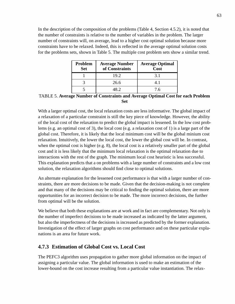
63

In the description of the composition of the problems (Table 4, Section 4.5.2), it is noted thatthe number of constraints is relative to the number of variables in the problem. The largernumber of constraints will, on average, lead to a higher cost optimal solution because moreconstraints have to be relaxed. Indeed, this is reflected in the average optimal solution costsfor the problems sets, shown in Table 5. The multiple cost problem sets show a similar trend.

With a larger optimal cost, the local relaxation costs are less informative. The global impact ofa relaxation of a particular constraint is still the key piece of knowledge. However, the abilityof the local cost of the relaxation to predict the global impact is lessened. In the low cost prob-lems (e.g. an optimal cost of 3), the local cost (e.g. a relaxation cost of 1) is a large part of theglobal cost. Therefore, it is likely that the local minimum cost will be the global minium costrelaxation. Intuitively, the lower the local cost, the lower the global cost will be. In contrast,when the optimal cost is higher (e.g. 8), the local cost is a relatively smaller part of the globalcost and it is less likely that the minimum local relaxation is the optimal relaxation due tointeractions with the rest of the graph. The minimum local cost heuristic is less successful.This explanation predicts that a on problems with a large number of constraints and a low costsolution, the relaxation algorithms should find close to optimal solutions.

An alternate explanation for the lessened cost performance is that with a larger number of con-straints, there are more decisions to be made. Given that the decision-making is not completeand that many of the decisions may be critical to finding the optimal solution, there are moreopportunities for an incorrect decision to be made. The more incorrect decisions, the furtherfrom optimal will be the solution.

We believe that both these explanations are at work and in fact are complementary. Not only isthe number of imperfect decisions to be made increased as indicated by the latter argument,but also the imperfectness of the decisions is increased as predicted by the former explanation.Investigation of the effect of larger graphs on cost performance and on these particular expla-nations is an area for future work.

4.7.3 Estimation of Global Cost vs. Local Cost

The PEFC3 algorithm uses propagation to gather more global information on the impact ofassigning a particular value. The global information is used to make an estimation of thelower-bound on the cost increase resulting from a particular value instantiation. The relax-

ProblemSet

Average Numberof Constraints

Average OptimalCost

1 19.2 3.1

3 26.6 4.1

5 48.2 7.6

TABLE 5. Average Number of Constraints and Average Optimal Cost for each ProblemSet

64

ation algorithms are also aggregating more global information in the form of the costs that arepropagated following value propagation. The difference between the algorithms, at this level,is that the PEFC3 algorithm is using its global information as a variable and value orderingheuristic and backtracks in attempt to find an even lower cost solution than the current. Therelaxation algorithms use the local relaxation cost information in order to select the candidateconstraints that will be searched over.

This observation suggests that if there is a relatively inexpensive source of global information,it will be a benefit to the relaxation algorithms to base the selection of candidate constraints onthat information. Texture measurements can be just such a source of information. Given, thelarge decrease in processing effort in the relaxation algorithms, another area of future work isthe improvement of the algorithms by the integration of texture measurements to supply anestimate of more global information. Such an integration with the relaxation algorithmsdetailed here would involve the selection of candidate constraints based on dynamically cal-culated texture measurements.4

4.7.4 The MC Algorithm

The variations on the MC algorithm performed poorly on the preliminary experiments so theywere not compared with the PEFC3 algorithm on the full set of problems. Given that the MCalgorithm is closely based on MinConflicts, this result is somewhat surprising.

It is known that repair-based algorithms need a “good” starting solution in order to performwell [Davis 94] . If the original solution is a local minima requiring two variables to changevalue to find a lower cost solution, then the repair will not succeed in moving from the startingsolution. The PNB algorithm, because it assigns the lowest cost value for a variable with nobacktracking, may find such a minima. We conducted experiments on all six problem setsusing a random starting solution. Cost performance was better, but still between 40% and 70%above optimal for 50 iterations.5 The MC algorithms did fewer consistency checks than eachof the other algorithms.

Given that the poor performance is not simply an artifact of the PNB starting solution, weanalysed the original data on each problem. Unfortunately, it was not the case that MC per-formed well on some problems and very poorly on others. In only a few problems in each setcould the MC performance be identified as good or poor.6 No consistent pattern relating per-formance difference to problem structure differences was in evidence.

4. In Chapter 5, we will use texture measurements to limit selection of outgoing constraints in much largergraphs (e.g 100 variables).

5. Experiments were also done with 100 and 200 iterations. There was little difference in cost performance.

6. We defined MC to have exhibited “good” performance when it was within 25% of the optimal cost and “poor”performance when it was above 75% of the optimal cost. About four problems per set could be categorized intoone of these two performance categories.

65

All the problems share the structure defined by the parameters of expected density, expecteddomain size, and satisfiability (see Table 4, Section 4.5.2). In the original PCSP experiments[Freuder 92] , these parameters were varied and each was found to have a statistically signifi-cant interaction with the number of consistency checks done in the complete algorithms inves-tigated. Because the algorithms were complete, no statistical analysis could be done on theinteraction between cost performance and these parameters. We postulate that such interac-tions do exist and further research, with a wider set of PCSPs, may give indications as tounderlying structural explanations for the poor performance of the MC algorithm.

4.8 Summary

This chapter has presented cache-based techniques for algorithms that instantiate the relax-ation schema. Three algorithms were created and two of them fared well in empirical compar-ison to the best algorithm for PCSPs. Due to the exponential time and space complexity ofthese algorithms, we do not view it likely that they will be applicable to any problemsapproaching the complexity of real-world problems. However, our approach allows specifica-tion of relaxation algorithms tailored to the time pressures and constraint types of the problemdomain. In the following chapter, we investigate such limited algorithms in the domain ofschedule optimization.

66

67

Chapter 5 Relaxation-BasedEstimation of the Impactof Scheduling Decisions

In this chapter, we demonstrate how relaxation-based methods can be used for estimating theimpact of scheduling an activity at a particular start time. We discuss job shop scheduling andthe constraint-based representation for such problems. This is necessary background for theelucidation of the estimation algorithms. Three texture-based estimation algorithms are pro-posed and compared against a baseline estimator on a set of medium-sized scheduling prob-lems (i.e. 100 activities, 5 resources).

5.1 Estimating the Impact of a Scheduling DecisionRevisited

In Chapter 2 (Section 2.5.4), we discussed techniques to estimate the global impact of assign-ing an activity to a start time. The key point in that work is that when attempting to schedulean activity, it is desirable to know the impact that assigning a start time will have on the over-all schedule cost. Dynamically calculated estimates have been shown to be superior to staticor dispatch rule based estimates in a number of situations [Sadeh 91] . Estimates will be cal-culated many times during scheduling, so we require the calculation to be efficient.

GERRY [Zweben 92] uses the number of local conflicts as an estimate for the global conflictscreated by an assignment. In contrast, MICRO-BOSS [Sadeh 91] propagates the changes inthe marginal cost to unscheduled activities. The method for identification of the best reserva-tions for an order is applicable only to the cost model used in the experimental problems. Fur-thermore, the propagation of information occurs only within an order. Potential increase incosts caused by interaction with other orders via resource constraints are not taken intoaccount. Earlier work on the propagation of preferences through a temporal constraint graphhas shown that the complexity of full propagation is prohibitive [Sadeh 89] . The preferencepropagation only addressed temporal constraint graphs and so, like the marginal cost propaga-tion in MICRO-BOSS, it to could not aggregate preference information over resource con-straints. The only example of which we are aware of using both inter- and intra-orderinformation is the MRP-STAR system [Morton 86] . The iterative calculation used is expen-sive and does not scale-up well to multiple resources and activities.

68

We believe that the ability to efficiently, accurately estimate the cost of scheduling decisions isa key to finding good schedules. Further, we hypothesize that the ability to dynamically selectthe subgraph over which cost gathering will be done, independent of constraint type and onthe basis of texture measurements, will improve the accuracy and efficiency of estimates.

We model the sources of cost in a schedule by the cost of relaxations necessary to satisfy con-straints. We, then, estimate the impact of the assignment of a value by the value and cost prop-agation phase of our relaxation schema. The generality of the schema allows us to aggregateinformation from all parts of the graph (that is, via any type of constraint) and the ability tospecify the actions at the decision points allows us to integrate heuristic decision making tominimize the overhead associated with full propagation.

5.2 Job Shop Scheduling

The job shop scheduling problem is a common, NP-complete [Garey 79] problem in the liter-ature [Fox 87] [Sadeh 91] [Nuitjen 93] [Davis 94] . The basic format is as follows:

Given:

• A set of orders where each order has a release date and a due date.• A process plan for each order containing one or more activities with precedence relation-

ships among the activities in the order and defining resources required by each activity.• A set of unit capacity resources.

Assign a start time to each activity such that:

• All precedence relationships are maintained.• No resource is used by more than one activity at any time point.1

5.2.1 A Constraint Model for Job Shop Scheduling

A number of authors [Fox 87] [Sadeh 91] [Ijcai 93] have approached job shop schedulingby using constraints to represent both the precedence relationships and the resource require-ments of activities. Each activity is represented by combinations of variables and constraints.

Our constraint model will build on the model used in the ODO scheduler [Davis 94] . In thissection we present an overview of the activity-level representation. The following sectionswill define the variable and constraints types introduced here. A diagram of two activities thatrequire the same resource is shown in Figure 24.

1. Most scheduling models define a scheduling horizon, a time granularity, and a number of time points withinthe horizon.

69

Figure 24. Schematic Diagram of The Activity Representation

Each activity is composed of three variables: StartTime and EndTime which are IntervalVari-ables and Resource which is a ResourceRequestVariable. The StartTime and EndTime vari-ables are connected by a TemporalConstraint. All three variables within an activity areconnected by a ResourceConstraint. Figure 24 also shows constraints between activities. TheTemporalConstraints are used to represent the precedence constraints by connecting Interval-Variables in different activities of the same order. The InterResRequestConstraint connectsResourceRequestVariables, in different activities, that use the same resource. These variableand constraint types can be divided into those representing the temporal dimension and thoserepresenting the resource dimension.

5.2.2 Temporal Variables and Constraints

An IntervalVariable has a value that is a time point. The domain is represented as a closedinterval of time points, indicating that the variable can take on any value in that intervalincluding the end points.

A TemporalConstraint is used to express a precedence constraint between two variables. Thebasic precedence constraint in job shop scheduling specifies that activity, Aj, occurs afteranother activity, Ai, has completed. For activities Ai and Aj (Figure 25), we specify that End-Timei + α = StartTimej, where α ≥ 0. We represent α by the value of the constraint. The valueis an interval of time points where each time point in the interval is a possible value for α.2

We link the EndTimei with the StartTimej via a TemporalConstraint, TC1. The value of TC1 is[0, ∞] as shown. To satisfy TC1, the difference between the value of the StartTime of Aj andthe value of EndTime of Ai must be an element of the interval value.

2. Equivalently, any element of the interval value is an acceptable difference between the values of the con-strained variables.

Activity1

Activity2

Variables

IntervalVariable

ResourceRequestVariable

Constraints

TemporalConstraint

InterResRequestConstraint

ResourceConstraint

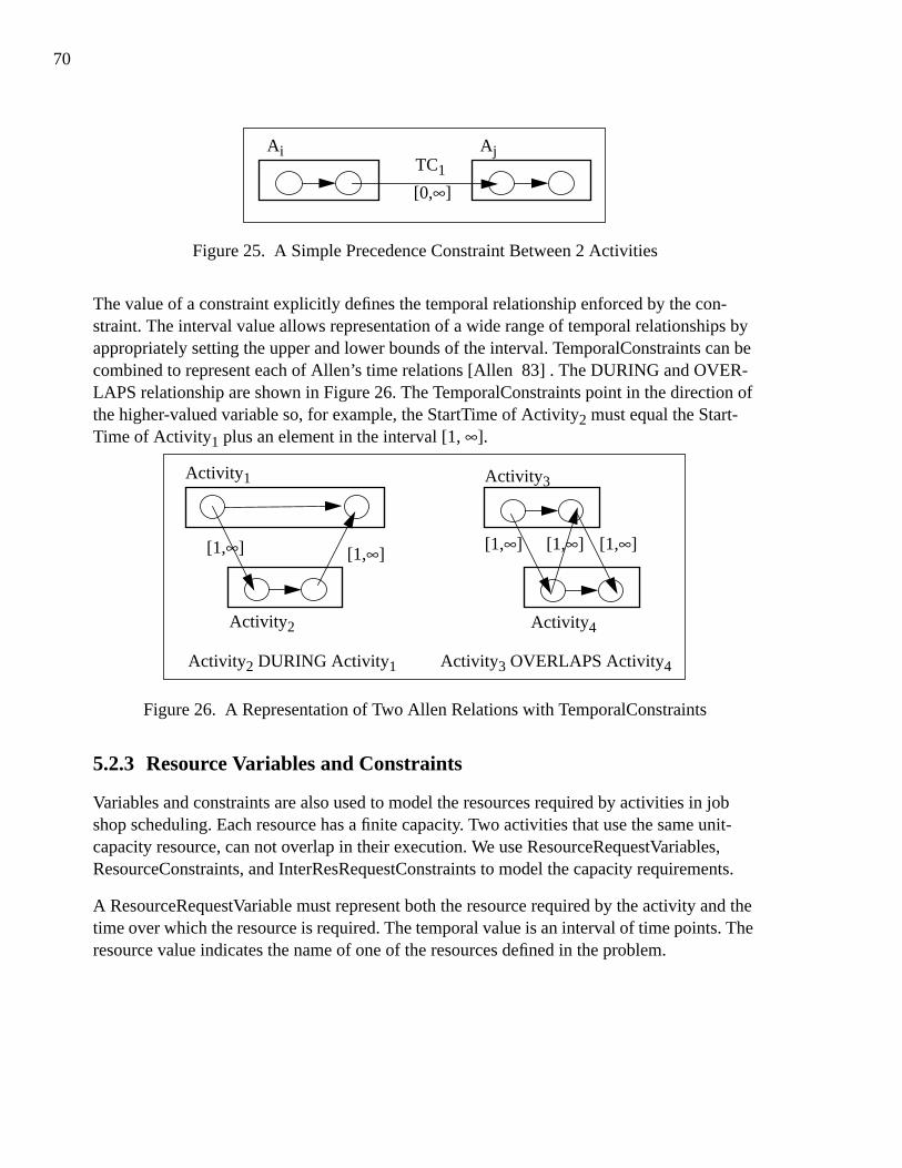
70

Figure 25. A Simple Precedence Constraint Between 2 Activities

The value of a constraint explicitly defines the temporal relationship enforced by the con-straint. The interval value allows representation of a wide range of temporal relationships byappropriately setting the upper and lower bounds of the interval. TemporalConstraints can becombined to represent each of Allen’s time relations [Allen 83] . The DURING and OVER-LAPS relationship are shown in Figure 26. The TemporalConstraints point in the direction ofthe higher-valued variable so, for example, the StartTime of Activity2 must equal the Start-Time of Activity1 plus an element in the interval [1, ∞].

Figure 26. A Representation of Two Allen Relations with TemporalConstraints

5.2.3 Resource Variables and Constraints

Variables and constraints are also used to model the resources required by activities in jobshop scheduling. Each resource has a finite capacity. Two activities that use the same unit-capacity resource, can not overlap in their execution. We use ResourceRequestVariables,ResourceConstraints, and InterResRequestConstraints to model the capacity requirements.

A ResourceRequestVariable must represent both the resource required by the activity and thetime over which the resource is required. The temporal value is an interval of time points. Theresource value indicates the name of one of the resources defined in the problem.

Ai Aj

[0,∞]

TC1

Activity1

Activity2

[1,∞] [1,∞]

Activity2 DURING Activity1

Activity3

Activity4

[1,∞] [1,∞]

Activity3 OVERLAPS Activity4

[1,∞]

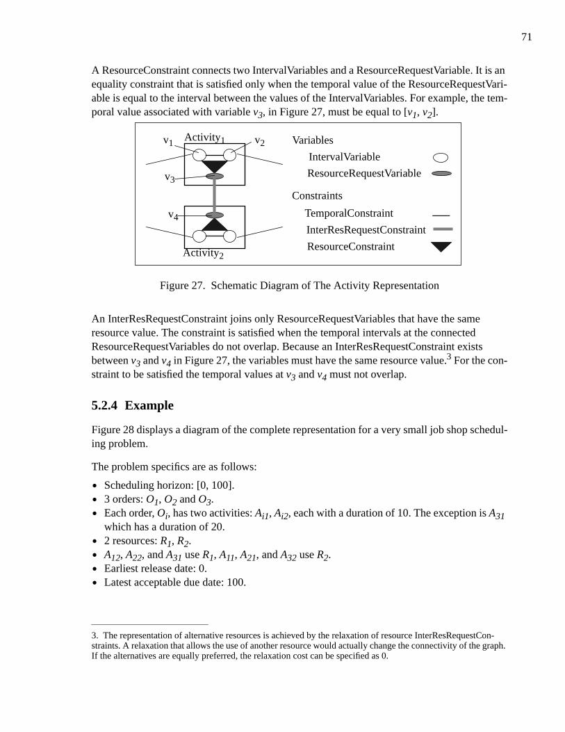
71

A ResourceConstraint connects two IntervalVariables and a ResourceRequestVariable. It is anequality constraint that is satisfied only when the temporal value of the ResourceRequestVari-able is equal to the interval between the values of the IntervalVariables. For example, the tem-poral value associated with variable v3, in Figure 27, must be equal to [v1, v2].

Figure 27. Schematic Diagram of The Activity Representation

An InterResRequestConstraint joins only ResourceRequestVariables that have the sameresource value. The constraint is satisfied when the temporal intervals at the connectedResourceRequestVariables do not overlap. Because an InterResRequestConstraint existsbetween v3 and v4 in Figure 27, the variables must have the same resource value.3 For the con-straint to be satisfied the temporal values at v3 and v4 must not overlap.

5.2.4 Example

Figure 28 displays a diagram of the complete representation for a very small job shop schedul-ing problem.

The problem specifics are as follows:

• Scheduling horizon: [0, 100].• 3 orders: O1, O2 and O3.• Each order, Oi, has two activities: Ai1, Ai2, each with a duration of 10. The exception is A31

which has a duration of 20.• 2 resources: R1, R2.• A12, A22, and A31 use R1, A11, A21, and A32 use R2.• Earliest release date: 0.• Latest acceptable due date: 100.

3. The representation of alternative resources is achieved by the relaxation of resource InterResRequestCon-straints. A relaxation that allows the use of another resource would actually change the connectivity of the graph.If the alternatives are equally preferred, the relaxation cost can be specified as 0.

Activity1

Activity2

Variables

IntervalVariable

ResourceRequestVariable

Constraints

TemporalConstraint

InterResRequestConstraint

ResourceConstraint

v1 v2

v3

v4

72

Figure 28. Constraint Representation of a Simple Job Shop Scheduling Problem

5.2.5 Constraint Relaxation in Scheduling

As discussed in Chapter 1 (Section 1.2.3) and Chapter 2 (Section 2.5), scheduling is an opti-mization problem on criteria such as tardiness, inventory, and throughput. We explicitlymodel the sources of cost in a scheduling problem with relaxable constraints. Previous workin ISIS and MICRO-BOSS schedulers has taken this approach. For example, due date con-straints could be relaxed up to the latest acceptable due date for the order. Our general con-straint relaxation work can be applied to not only model optimization criteria like tardinessand inventory costs but also sophisticated resource-based trade-offs. For example, it may bethat a particular activity has different possible durations. The long duration corresponds tousing a machine at a slow speed with minimal machine wear, whereas the small duration cor-responds to using the machine at high speed with increased wear. The long duration activitycosts less (due to maintenance costs). This can be represented as a relaxable duration con-straint where the RelaxationCost function is inversely proportional to the duration. We believe

A31

A21

A32

A22

[0, ∞]

[0, ∞]

[0, ∞]

[10, 10]

[10, 10] [10, 10]

[20, 20]

Release: 0

R2 R1

A11 A12[0, ∞]

[10, 10] [10, 10]

Latest: 100

R1

R1

R2

R2

[0, ∞]

[0, ∞]

[0, ∞][0, ∞]

[0, ∞]

A31

IntervalVariable

ResourceRequestVariableTemporalConstraint

InterResRequestConstraintResourceConstraint

Activity

73

that most (or all) currently used optimization criteria can be modeled in this fashion and that ithas the generality to represent many more criteria. Further research is required to assess thevalidity of this belief.

We only address temporal constraint relaxation in this dissertation. For the problems studiedhere, all other constraint types are non-relaxable. We leave the definition of complex costmodels via relaxation of other constraint types for future work. TemporalConstraints are basedon the value of the constraint represented by an interval as described above (Section 5.2.2).Relaxation is simply a widening of this interval. The GenerateRelaxation function, therefore,returns a set of constraints that have a wider interval value than the original constraint. Foreach TemporalConstraint, the RelaxationCost function is defined to be a function of the wid-ening of the constraint.

5.2.6 Extending the Example

Figure 29 shows the problem from Figure 28 with the addition of relaxable constraints model-ing tardiness and inventory costs. The non-relaxable constraints have been removed from thediagram for clarity. We model tardiness with a TemporalConstraint between the EndTime ofthe last activity in an order and an IntervalVariable representing the due date. The value of theconstraint is [0, ∞]. If the EndTime is less than or equal to the due date, no relaxation need bedone. Otherwise, the constraint interval is expanded, incurring some cost.

Figure 29. Optimization Constraints on the Example Scheduling Problem

A31

A21

A32

A22Release: 0

A11 A12

Due Date: 80

Due Date: 60

C33: [0, 0]

C23: [0, 0]

C13: [0, 0]

C32: [0, 0]

C31: [0, 0]

C21: [0, 0]

C22: [0, 0]

C11: [0, 0]

C12: [0, 0]

IntervalVariable

ResourceRequestVariableRelaxable TemporalConstraint

A31 Activity

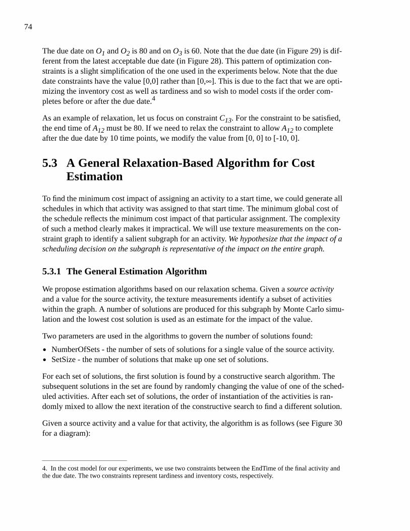
74

The due date on O1 and O2 is 80 and on O3 is 60. Note that the due date (in Figure 29) is dif-ferent from the latest acceptable due date (in Figure 28). This pattern of optimization con-straints is a slight simplification of the one used in the experiments below. Note that the duedate constraints have the value [0,0] rather than [0,∞]. This is due to the fact that we are opti-mizing the inventory cost as well as tardiness and so wish to model costs if the order com-pletes before or after the due date.4

As an example of relaxation, let us focus on constraint C13. For the constraint to be satisfied,the end time of A12 must be 80. If we need to relax the constraint to allow A12 to completeafter the due date by 10 time points, we modify the value from [0, 0] to [-10, 0].

5.3 A General Relaxation-Based Algorithm for CostEstimation

To find the minimum cost impact of assigning an activity to a start time, we could generate allschedules in which that activity was assigned to that start time. The minimum global cost ofthe schedule reflects the minimum cost impact of that particular assignment. The complexityof such a method clearly makes it impractical. We will use texture measurements on the con-straint graph to identify a salient subgraph for an activity. We hypothesize that the impact of ascheduling decision on the subgraph is representative of the impact on the entire graph.

5.3.1 The General Estimation Algorithm

We propose estimation algorithms based on our relaxation schema. Given a source activityand a value for the source activity, the texture measurements identify a subset of activitieswithin the graph. A number of solutions are produced for this subgraph by Monte Carlo simu-lation and the lowest cost solution is used as an estimate for the impact of the value.

Two parameters are used in the algorithms to govern the number of solutions found:

• NumberOfSets - the number of sets of solutions for a single value of the source activity.• SetSize - the number of solutions that make up one set of solutions.

For each set of solutions, the first solution is found by a constructive search algorithm. Thesubsequent solutions in the set are found by randomly changing the value of one of the sched-uled activities. After each set of solutions, the order of instantiation of the activities is ran-domly mixed to allow the next iteration of the constructive search to find a different solution.

Given a source activity and a value for that activity, the algorithm is as follows (see Figure 30for a diagram):

4. In the cost model for our experiments, we use two constraints between the EndTime of the final activity andthe due date. The two constraints represent tardiness and inventory costs, respectively.

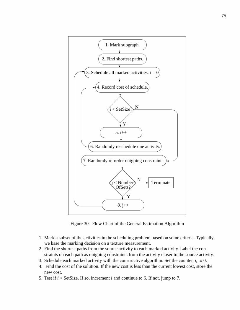
75

Figure 30. Flow Chart of the General Estimation Algorithm

1. Mark a subset of the activities in the scheduling problem based on some criteria. Typically,we base the marking decision on a texture measurement.

2. Find the shortest paths from the source activity to each marked activity. Label the con-straints on each path as outgoing constraints from the activity closer to the source activity.

3. Schedule each marked activity with the constructive algorithm. Set the counter, i, to 0.4. Find the cost of the solution. If the new cost is less than the current lowest cost, store the

new cost.5. Test if i < SetSize. If so, increment i and continue to 6. If not, jump to 7.

5. i++

i < SetSize?

Terminate

N

Y

4. Record cost of schedule.

2. Find shortest paths.

1. Mark subgraph.

3. Schedule all marked activities. i = 0

6. Randomly reschedule one activity.

7. Randomly re-order outgoing constraints.

8. j++

j < Number-

Y

OfSets?

N

76

6. Randomly change the value of a scheduled activity, loop to 4.7. Randomly re-order the outgoing constraints at the source activity.8. Test if counter j < NumberOfSets. If so, loop to 3. If not, terminate.

A number of points arise from the specification of this general algorithm:

• The algorithm operates on activities rather than variables. The constraints within an activ-ity are not relaxable. We can treat the graph as a network of activities and constraints ratherthan as a network of variables and constraints. This abstraction realizes a three-fold reduc-tion in the number of nodes in the graph.

• In step 3, all the activities in the subgraph are assigned a start time. A constructive algo-rithm is used to find a consistent solution for the subgraph. See Section 5.3.3 below.

• The outgoing constraints at the source activity are randomly re-ordered before each use ofthe constructive algorithm. The solutions generated by randomly changing activity assign-ments are relatively close together in the search space. By re-ordering the outgoing con-straints, we change the order of instantiation of the activities and so move to a remoteposition in the search space. We gather further random solutions in the new area.

• The total number of solutions found for each candidate value of the source activity is Set-Size × NumberOfSets.

• The cost at an activity is a texture measurement in itself. It is a measurement of the con-straint tightness surrounding the activity. The higher the cost, the larger the necessaryrelaxation and therefore, the tighter the constraints were before relaxation. By aggregatingthese costs for each value of the source activity, we are able to find an estimate of the globalimpact of the assignment.

It remains to specify the following techniques before turning to the specific algorithms:

• Identifying the subgraph.• Finding the solution with constructive search.• Calculating the cost of the subgraph schedule.

5.3.2 Finding a Subgraph

The preprocessing on the graph consists of the marking a subset of the activities in the graphand identifying the shortest path between the source activity and each marked activity. Eachconstraint on this path is defined to be an outgoing constraint of the activity that is closer tothe source activity. Each path of outgoing constraints, beginning at the source activity, termi-nates at a marked activity. The criteria for marking activities varies among the algorithms.

Though all the marked activities appear in the subgraph, there may also be some unmarkedactivities in the subgraph (i.e. activities on the shortest path between the source activity and amarked activity). Only the marked activities are scheduled by the constructive algorithm.

77

More formally, the entire scheduling problem is represented as a graph G = (V, E), where V isa set of vertices (activities) and E is a set of edges (constraints). The preprocessing finds a sub-graph G´ = (V´, E´), V´ ⊆ V, E´ ⊆ E. All the elements in V that are marked are also in V´, how-ever there may be some elements in V´ that are not marked.

5.3.3 The Constructive Search Algorithm

To find the first solution, we begin with the source activity assigned to a candidate value and asubgraph connected by the outgoing constraints. The constructive algorithm is as follows:

1. Value propagate along all non-relaxable constraints (in the whole graph, G) to prune incon-sistent values in the domain of other activities.

2. Propagate control from the source activity, along one of the outgoing constraints to theadjacent activity.

3. Assign the activity to the earliest consistent start time and value propagate along all non-relaxable constraints in G. If no such value exists return to previous activity (go to 5) withthe backtrack flag set.

4. If there are outgoing constraints that control propagation has not visited, go to 2. Other-wise, return control to the previous activity (go to 5) with the backtrack flag un-set.

5. At the previous activity, if the backtrack flag is set, prune the current value from thedomain, go to 3. Otherwise, go to 4.

5.3.3.1 Value and Control Propagation

In all the previously presented relaxation algorithms, a variable is instantiated and the controland value propagation proceed together to a connected variable along an outgoing constraint.As noted in Chapter 3 (Section 3.2.1), value and control propagation are more generally inde-pendent.

When an activity is assigned, value propagation proceeds along all temporal and resource con-straints (all constraints, c, such that c ∈ E). Elements in the domain of adjacent variables arepruned if they are not consistent with the assignment. If a value is pruned, the domains ofother activities may also need to be pruned. The value propagation may proceed to, at most,all activities in the graph (all activities, a, such that a ∈ V). The value propagation ensures thatwhen a marked activity is assigned a value, that value is consistent with previous assignments.

Control is propagated along each outgoing constraints in some sequence and the activitiesreached are instantiated to a consistent value. We arbitrarily choose the lowest consistentvalue in the domain. The only exception to this is the constructive search with the Contention/Reliance algorithm (see Section 5.5.6.2). If no consistent value exists, chronological back-tracking is done.

78

5.3.3.2 Backtracking

Chronological backtracking is initiated when an activity has no consistent value to which itcan be assigned. That activity returns control to the previous activity with a flag indicating thefailure. The previous activity unassigns itself and undoes the effect of the value propagation.5

The activity then chooses another consistent value and performs value and control propaga-tion as usual. If the activity does not have any more consistent values, it returns control to thenext-most recently assigned activity, indicating the need to backtrack.

Backtracking is, at worst, exponential in time complexity and so is prohibitively expen-sive.The expense is compounded by that fact that the backtracking algorithm may be used anumber of times to find an solution for each value of the source activity. It is critical that verylittle or no backtracking occur.

5.3.3.3 The Relaxation Schema

In terms of our relaxation schema, we have the following specification for each heuristic deci-sion point:

• Source activity: Chosen a priori.• Candidate values: All consistent values. The Monte Carlo simulation randomly samples the

candidate values in finding the subsequent solutions.• Outgoing constraints: All constraints identified in the preprocessing step.• Candidate constraints: All outgoing constraints are non-relaxable, therefore only candidate

constraint at each outgoing constraint is simply the constraint itself.• Value-commitment: We are gathering costs; no value-commitment is done.

5.3.4 Calculating the Cost of a Subgraph Solution

Relaxable constraints are the source of cost in our model of schedule optimization, thereforethe cost calculation is based on an estimate of the necessary relaxations. Cost propagation isperformed after a solution has been found for the subgraph, at which point control is at thesource activity. The cost propagation passes control along the outgoing constraints and at eachmarked activity the cost of all attached, relaxable constraints is calculated. The sum is thenpropagated back toward the source activity where it is summed with all the other costs.

Each relaxable constraint is marked when its cost is calculated. This prevents the doublecounting of relaxation costs for constraints connecting two marked activities. After all markedactivities have calculated their local cost, the cost of any relaxable constraints that have notbeen marked is calculated. This cost is added to the sum of the local costs. The final sumreflects an estimate of the cost of the whole graph given the partial schedule.

5. In undoing the effects of the value propagation, the activity must restore the graph to the state it was in beforethe activity was assigned the previous value. We use a context stack to cache search states to which we maybacktrack. There is no search involved in undoing the value propagation of a previous assignment.

79

Because we are scheduling a subset of the activities in the full problem, we have the followingthree cases in the calculation of the relaxation cost of a single relaxable constraint.

1. Both connected activities have been scheduled.2. Only one of the activities has been scheduled.3. Neither activity has been scheduled.

In the first case, the constraint simply relaxes itself to allow the two assigned values to be con-sistent. In the second case, the domain of the unassigned activity is examined and, of theremaining consistent start times, the start time that will maximize the relaxation cost is chosenas a temporary value. Relaxation is then performed with this temporary value. Finally, if nei-ther activity is assigned, the domains of each activity is analyzed and the start times that willmaximize the relaxation cost of the constraint are used. For example, if the constraint has aninterval value of [0,∞], the maximum cost occurs when the activity at the lower end isassigned to its maximum value and the other activity is assigned to its minimum value.

In the latter two cases we examine the domains of the unscheduled activities to find a worstcase estimate of the relaxation cost incurred at the constraint. We choose the maximum cost inorder to find an upper bound on the impact of the value assigned to the source activity. It ispossible however, that the domain of one of the connected activities is empty; that is, there areno consistent candidate values. This occurs when the activity is not one of the marked activi-ties and is not assigned. In that case, we use the worst possible case relaxation cost based onthe original domains of the activities.

We choose the maximum cost relaxation when we have no other information about the relax-ation to be made for two reasons.

1. We want the estimates to be an upper bound on cost of the relaxations. A true upper boundwould allow the estimates to be used in other algorithms where a choice must be madebetween activities and not simply about values within an activity. For example, we maywant to make the activity/value selection a single decision point and so must judge betweena number of activity/value tuples to make an assignment. Unfortunately, even using theworst case costs does not guarantee a true upper bound because the subgraph solution maynot be a partial solution to the larger graph (see Section 5.3.5).

2. A subgraph solution is not guaranteed to be a partial schedule for the whole problem. Byusing pessimistic estimates, we hope to counteract the likelihood that some of the cost esti-mate will be based on subgraph solutions that will not lead to an overall solution.

5.3.5 Partial Solutions vs. Solutions to the Subgraph

The constructive search algorithm finds solutions to the subgraph. The solutions are not neces-sarily partial solutions to the whole graph. It is possible that one or more of the unmarkedactivities will have empty domains in a solution found by the constructive search. Backtrack-ing only occurs when an attempt is made to schedule a marked activity and no valid start times

80

exist. Because the unmarked activities are not scheduled, an empty domain will not be recog-nized. This is the desirable behaviour because we are attempting to find a fast estimate of theimpact of a schedule decision rather than actually scheduling.

5.3.6 Complexity

If no backtracking is done, the general complexity of the algorithm depends on the value prop-agation. During the constructive algorithm, whenever an activity is assigned, value propaga-tion will, at most, visit all activities in the complete graph. The number of activitiesinstantiated during the constructive algorithm is, at most, the size of the subgraph. If there area total of n activities in the graph, and m activities in the subgraph, the value propagation has atime complexity of O(mn). The instantiation of the activities in the constructive search (withno backtracking) incurs an additional complexity of O(m) and the number of random assign-ments made after each backtracking solution is SetSize - 1. The whole loop is performedNumberOfSets times, therefore the overall complexity to find cost estimate for one value of anactivity is O(NumberOfSets × (mn + m + SetSize - 1)). If backtracking is necessary the worstcase complexity of constructive search is O(dm), where d is the maximum domain size.

5.4 The Cost Estimation Algorithms

There are four methods by which the subgraph is selected. The first method, the Depth algo-rithm, is used for a baseline estimate of the actual impact. We compare the other algorithms tothe Depth algorithm. The other three algorithms depend on texture measurements to identifythe activities with the largest effect on the cost of a candidate value at the source activity.

5.4.1 The Depth Algorithm

The Depth algorithm is used to establish a baseline cost estimate against which the other algo-rithms are compared. The algorithm is designed to choose a subset of activities based on sim-ple-minded criteria. The Depth algorithm marks all activities that are directly connected to thesource activity via a path of constraints of length L or less.

5.4.2 The TemporalOnly Algorithm

The TemporalOnly algorithm marks those activities that are connected to the source activityvia a path of temporal constraints. This has the effect of strictly restricting the size of the sub-graph over which solutions are found. In our experimental problems, there are a total of 5activities in an order and only the activities within an order are connected via temporal con-straints. The number of marked activities for the TemporalOnly algorithm is 4.

This algorithm is designed to estimate the impact of activity reservations in a way similar tothe marginal cost propagation in MICRO-BOSS. The algorithm should not be interpreted as are-implementation of marginal cost propagation as it is both less efficient and more general.

81

5.4.3 The TopCost Algorithm

The TopCost algorithm uses the expense texture measurement based on the maximum costthat might be incurred by an activity. As described below (Section 5.5.2), the RelaxationCostof the relaxable constraints is a function of the width of the relaxation and the weight (or Cost-Factor) of the constraint. Because the RelaxationCost varies directly with the CostFactor, thehigher the CostFactor of a relaxable constraint, the more potential effect it has on the overallschedule cost. We identify the expense of an activity as the sum of the CostFactors of its relax-able constraints. Intuitively, the more expensive activities have a large impact on the overallcost schedule and therefore provide an accurate estimation of the impact of an assignment.

For the TopCost algorithm, we use the expense texture measurement to identify and mark them most expensive activities (other than the source activity).6

5.4.4 The Contention/Reliance Algorithm

The Contention/Reliance algorithm uses a different texture measurement to identify activitieswith a large impact on the cost of a scheduling decision. The time intervals over which there isthe most contention for a resource and the activity that is most reliant on the resource for thattime interval are identified. These texture measurements were developed for and used as abasis of the activity ordering heuristic in MICRO-BOSS. In overview, we identify the m mostcontended for resource intervals and mark the activities most reliant on each interval.

The contention of an activity for a particular resource at a start time is defined in equation 3.

(3)

Where:

d´ is the domain of consistent candidate values at the activity.

|d´| is the size of the domain of consistent candidate values at the activity.

Using equation 3, we build a profile of the contention of an activity for a resource across allconsistent values of that activity. An activity with very few consistent values will have a highcontention (i.e. close to 1) for each of its consistent start times. We sum the profiles of eachactivity on a resource to form an aggregate resource contention profile. An aggregate resourcecontention profile is generated for each resource.

Based on an interval size equal to the average duration of an activity on a resource, we iden-tify the top m intervals in terms of high aggregate contention for any resource. For each inter-val, we identify the most reliant activity. The reliance of an activity is defined to be the areaunder its individual contention curve over the interval. The most reliant activity of an interval

6. The source activity may be one of the m most expensive activities. In this case, the next most expensive activ-ity is marked and the source activity is left unmarked.

Contention1d′=

82

is therefore the activity that contributed most to the aggregate resource contention. We markthe most reliant activity at each interval. If an activity is the most reliant activity on more thanone interval, we mark the activity and discard all but one of the intervals where it is most reli-ant. We then find the next most contended for intervals in order to bring the interval total backto m. This ensures that a total of m unique activities are marked.

The assignment of the source activity and the subsequent value propagation significantlyprunes the domains of some activities. Resource contention depends on the possible values ofeach unassigned activity, therefore the marking of the activities is performed for every valueof the source activity. This differs from the Depth, TemporalOnly, and TopCost algorithms,where the marked activities are independent of the value of the source activity.

5.4.5 Expectations

The performance of each algorithm will be evaluated in comparison to the baseline estimate.Assuming the baseline estimate is accurate (see Sections 5.7), we expect the following results.

• Controlling for subgraph size and parameter settings, we expect the TopCost algorithm andthe Contention/Reliance algorithm will outperform the TemporalOnly algorithm. The Tem-poralOnly texture measurement is not actually based on information indicating that theactivities have a large impact on a scheduling decision. We expect that the algorithms thatuse the extra information will perform better than the TemporalOnly algorithm. The perfor-mance comparison between the TopCost algorithm and Contention/Reliance algorithm isnot obvious prior to experimentation.

• We expect that, other settings being equal, the algorithms using larger graphs will outper-form the same algorithms on smaller graphs. With a larger number of activities with whichto make an estimate, it seems likely that the estimate will be more accurate.

• On graphs of the same size and within the same algorithm, we expect that estimates will besuperior when more solutions are generated with the constructive algorithm. The construc-tive solutions for a single source activity value use different orderings of marked activitiesand therefore should sample a wide range of locations in the search space. Conversely, therandomly generated solutions will cluster around the constructive solution from which theyare produced. Therefore, with a low number of constructive solutions and a lot of randomsolutions, the quality of the sampling of the search space will be less than with a high num-ber of constructive solutions and fewer random solutions.

5.5 Experiments

We now turn to specific experiments that were run. We first describe the experimental prob-lems, the cost model used, and the evaluation criteria for the algorithms. This is followed witha discussion of how the source activity and its candidate values were selected. Finally, wepresent an analysis of the accuracy of the baseline estimates and a discussion of the parametersettings used for each algorithm.

83

5.5.1 Experimental Problems

The experiments use problems in eight problem sets created by [Sadeh 91] . Each set contains10 scheduling problems and each problem contains 20 orders, 5 activities per order, and 5resources. Each activity in an order uses a different resource. The main variables in the gener-ation of the problems were the average tightness of due dates, the range of due dates, and thenumber of bottleneck resources.

• The average tightness is used to set the due date of each order. The higher the tightness, theless likely it is that an order can finish on time. Problems in Sets 1, 2, 5, and 6 have a looseaverage tightness, while the rest have a tight average tightness.

• The range of due dates specifies the variation in due dates across orders. With a wide range,each order may have a due date far from the due dates of other orders. The narrower therange the more likely that due dates will be close together, increasing the likelihood of con-flict among orders. Problems in Sets 1, 3, 5, and 7 have a wide due date range, while theother problems have a narrow due date range.

• A bottleneck resource is one for which there is a high contention over some time interval.A problem with more bottleneck resources will typically be more difficult to schedule. Inhalf of the problems sets (Sets 5 through 8) there are two resources for which there is a highcontention over the entire scheduling horizon, where as in the rest of the problem sets thereis only one such resource.

5.5.2 Cost Model

The optimization criteria considers both tardy costs and inventory or holding costs. The totalschedule cost is the sum of the tardy and holding costs for each order. It is the same cost modelused in MICRO-BOSS [Sadeh 91] .

The tardy cost for an order is the product of the TardyCostFactor and the difference betweenthe completion date and the due date. If an order is completed early, no tardy cost is incurred.Each order has an individually specified TardyCostFactor. The tardy cost for order i, TARDi, isas follows:

(4)

Where:

Ci is the time of completion of the last activity in order i

ddi is the due date for order i

The holding costs represent the cost of storing raw materials and intermediate products. AHoldingCostFactor is defined for each activity. The holding cost for a activity is the product ofits HoldingCostFactor and the difference between the completion time of the order and the

TARDi TardyCostFactori max 0 Ci ddi−,( )×=

84

start time of the activity. If the order finishes early, the holding cost is the product of the Hold-ingCostFactor and the difference between the due date and the start time of the activity. Theholding cost for an order i, HOLDi, is the sum of the holding costs for its constituent activities.

(5)

Where:

ni is the number of activities in order i

STij is the start time of activity j in order i

The holding cost for an order can be equivalently re-written as:

(6)

To represent this cost model via relaxable constraints, we define a CostFactor (or weight) ateach constraint and specify that the RelaxationCost is the product of the CostFactor and theamount that the interval is widened.

We add three types of temporal constraints to the problem representation:

1. A TardyConstraint connects the final activity of each order to a fixed variable with thevalue of the due date of the order. The CostFactor of the constraint is the TardyCostFactorfor the order. The interval value of the constraint is [0, ∞]. The relaxation cost of a Tardy-Constraint for an order is equivalent to equation 4.

2. A HoldingConstraint connects the start time of each activity in an order to the end time ofthe final activity in the order. The CostFactor for the constraint is the HoldingCostFactorfor the activity. The interval value for a HoldingConstraint is [−∞, 0] reflecting the fact thatcost will be incurred only if the start time of the task is less than the completion time of theorder.7 The sum of the relaxation costs of the HoldingConstraints for an order is equivalentto the first addend in equation 6.

3. An EndHoldingConstraint connects the final activity in the order to the variable represent-ing the due date. The CostFactor is the sum of the HoldingCostFactors for each activity inthe order and, as with HoldingConstraints, the interval value is [−∞, 0]. The relaxation costof the EndHoldingConstraint is equivalent to the final addend in equation 6.

7. With non-zero activity durations, it is clearly impossible to have the start times of activities in an order greaterthan or equal to the completion time for that order. Therefore, all holding cost constraints will have to be relaxedto some extent. A zero cost schedule is impossible.

HOLDi HoldingCostFactorij max Ci ddi,( ) STij−[ ]×j 1=

ni

∑=

HOLDi HoldingCostFactorij Ci STij−( )×[ ]j 1=

ni

∑ +=

Hj 1=

ni

∑ oldingCostFactorij

max 0 ddi C− i,( )×

85

5.5.3 Evaluation Criteria

Estimations of the cost of the candidate values of an activity are used to establish the valueordering heuristic in typical scheduling algorithms. It is not necessary that a cost estimationalgorithm find estimations that are close to the actual cost. Rather we require that the sameordering be created given the estimated costs as would be created if the actual costs wereavailable. Because the cost estimates are only compared to each other in forming the ordering,a good estimator finds costs such that the difference between the actual costs and the estimatedcosts is constant across all candidate values. Such an estimator will produce a cost curve thatis a vertical translation of the actual cost curve. We define the estimation gap, EstGap, of analgorithm on a single problem as follows:

(7)

Where:

σ is the standard deviation of a vector.

CostDifferenceVector is a vector defined by equation 8.

(8)

Where:

BaselineVector is the costs calculated by the Depth algorithm across all candidate values.

EstVector is the costs calculated by the estimation algorithm across all candidate values.

The estimation gap is a measure of the variability in the difference in estimates between thebaseline and the algorithm being evaluated. A value of 0, corresponding to a constant differ-ence between the baseline and the estimations, is optimal.

The complexity analysis above indicates that the number of assignment and the number ofactivities visited during cost propagation are the relevant factors. Therefore, to compare algo-rithms on time performance we use the ChangeActivity statistic. It counts the number timesthat an activity is assigned to some value plus the number of activities that are visited in thevalue propagation during the backtracking algorithm. On this basis the forming of a solutionby the random changing of the value of an activity will increment the ChangeActivity statisticby one. In contrast, the generation of a solution with the backtracking algorithm will incre-ment the ChangeActivity count by, at most, the number of marked activities times the totalnumber of activities in the schedule.8 The worst case occurs when each instantiation of amarked activity requires that all activities in the graph are visited by value propagation.

8. Again, we assume that no backtracking is done.

EstGap σ CostDifferenceVector( )=

CostDifferenceVector BaselineVector EstVector−=

86

Note that each of the texture measurements incur some processing time. We will not includethe processing time needed to identify the subgraphs in the ChangeActivity statistic as wewant to focus on the work done in finding the estimation rather than in selecting the subgraph.This is typically a valid abstraction as the differences in effort in forming the subgraphbetween texture-based algorithms are small.

5.5.4 The Source Activity

5.5.4.1 Selecting the Source Activity

To this point we have not specified how the source activity is selected. The estimation algo-rithms are designed to estimate the cost of the scheduling options of any activity, however, anartifact of the experimental problems prevents us from using random selection.

The scheduling problems were created so that only the first and last activities in an order havenon-zero CostFactors on their relaxable constraints. Though the underlying cost model allowa holding cost to be specified for each activity, in the experimental problems the holding costsfor the entire order are introduced by the first activity. The holding cost constraints for allother activities have a CostFactor = 0. The tardy costs only depend on the end time of the finalactivity. Therefore, the middle three activities in an order do not have an impact of the cost ofthe schedule, except indirectly, via interactions with other activities. Furthermore, all theactivities using a bottleneck resource have the same relative positions in their respectiveorders. For example, the third activity in each order may use the bottleneck resource. This pat-tern of resource use is not used for non-bottleneck resource activities. With this problem struc-ture, it is possible in some problems to find an activity that has no non-zero cost relaxableconstraints and, more seriously, that has few or no neighboring activities with non-zero costrelaxable constraints. In such a situation, the cost estimate of one of our algorithms (the Depthalgorithm, Section 5.5.5) would be based solely on the worst case costs of all relaxable con-straints. The algorithm would find a constant-value cost curve. This is clearly not desired asour results depend on the accuracy of the baseline estimates found by the Depth algorithm.

To avoid this situation, we use the expense texture measure (see Section 5.4.3) to identify themost expensive activity. We use the most expensive activity as the source activity in all prob-lems. This activity has non-zero cost relaxable constraints and so will either be the first or lastactivity in an order. If the activity uses a bottleneck resource, all other activities using theresource will have non-zero cost relaxable constraints (they too will be first or last activities).If the source activity does not use a bottleneck resource, between 25% and 66% of all con-nected activities will have non-zero cost relaxable constraints. The choice of the most expen-sive activity is motivated by the desire to ensure the accuracy of the baseline estimates.

87

5.5.4.2 Selecting Candidate Values for the Source Activity

In a scheduling situation where none of the other activities have assignments, all values in thedomain of the source activity are potential assignments. For the purpose of our experiments,we gather a cost estimate for every tenth value of the source activity, starting with the loweststart time. The size of this candidate value set is approximately 30. Sampling the domain ofthe source activity allows us to build a coarse-grained cost curve over the candidate values.More fine-grained cost estimates can then be made around the lower cost values. For thepresent experiments, we form only the coarser cost curve.

5.5.5 The Depth Algorithm

The depth algorithm requires a specification of the value of L, the length of paths radiatingfrom the source activity. We experimented with L = 2 corresponding to a subgraph of approx-imately 80 activities (80% of the entire graph). With a subgraph of this size, significant back-tracking is noted in the constructive search. No solutions could be found in a reasonable time.9

Therefore, we use a value of L = 1. The subgraph is composed of 20 or 21 activities (20% ofthe whole graph), plus the source activity in our experimental problems.

Figure 31. The Average Cost Found by the Depth Algorithm with L = 1 for the Problem Setswith 1 Bottleneck

9. The running time on a DECStation 5000/244 on a single problem is estimated to be over 640 hours.

78000

80000

82000

84000

86000

88000

90000

0 100 200 300 400 500

Average Cost

Number of Solutions

Problem Set 1Problem Set 2Problem Set 3Problem Set 4

88

In order to assess the accuracy of the estimate of the Depth algorithm, we ran a series ofexperiments on all problems. We set the SetSize parameter to 20 and varied the NumberofSetsfrom 1 to 25. Each set of solutions is composed of a single solution found by the constructivealgorithm and 19 randomly produced solutions based on the constructive solution. A total ofNumberOfSets × SetSize solutions are produced. The x-axis in our plots shows the total num-ber of solutions calculated for each problem in the set rather than the value of NumberOf-Sets.10 Figures 31 and 32 present the average cost for each problem set.

Figure 32. The Average Cost Found by the Depth Algorithm with L = 1 for the Problem Setswith 2 Bottlenecks

Two observations are made from Figures 31 and 32:

• The rate of reduction in the average cost lessens with the increase in the number of solu-tions. With 500 solutions (25 constructive solutions and 475 random solutions), the curvesin Figure 31 appear linear and in Figure 32 are close to linear. The small decrease in aver-age cost indicates that further iterations would decrease the cost only slightly.

• The average costs for the problems with 1 bottleneck are much larger than those for the 2bottleneck problems. Given the structure of the problems and the subgraph, if the sourceactivity requires a bottleneck resource, 19 of the activities in the subgraph also require thesame resource. Furthermore, due to the method by which the source activity is selected (seeSection 5.5.4.1), each of those 19 activities will have a non-zero cost impact on schedulingdecisions. If the source activity is not a bottleneck activity, fewer activities in the subgraphwill have non-zero cost impacts. Given that there are the same number of activities with

10. Because SetSize is 20, it is easy to show that the total number of solutions is simply 20 × NumberOfSets.

18000

20000

22000

24000

26000

28000

0 100 200 300 400 500

Average Cost

Number of Solutions

Problem Set 5Problem Set 6Problem Set 7Problem Set 8

89

non-zero impact, when the source activity is a bottleneck activity, a greater percentage ofthe activities with non-zero impact will be in the subgraph. With 2 bottlenecks the sourceactivity has a greater chance of being a bottleneck activity, therefore the worst case esti-mate will be used for fewer constraints, and the cost estimates will be lower.

Given these results, we adopt the parameter values of 20 and 25 for SetSize and NumberOf-Sets, respectively. The cost curves indicate that little significant change will occur to the aver-age costs with more iterations, however we do not have a measure of the accuracy of thebaseline estimates as found by the Depth algorithm. In our results section we will present theestimates of the texture-based algorithms in relation to the baseline estimates. We will returnthe issue of the accuracy of the baseline estimate in the discussion below (Section 5.7).

5.5.6 Parameter Settings for the Texture-Based Algorithms

The parameters that we vary in our experiments are the size of the subgraph over which theestimations are taken and the number and type of solutions that are found.

5.5.6.1 Subgraph Size

Of the three texture-based algorithms, the subgraph size can only be varied in the TopCost andContention/Reliance algorithms. The TemporalOnly algorithm selects all activities connectedvia a path of temporal constraints. In the experimental problems, only activities within anorder share temporal constraints, therefore, with only 5 activities per order, the size of the sub-graph is limited to 4 (not including the source activity).

For the TopCost and Contention/Reliance algorithm, we set the size of the subgraph to twodifferent values: 4 and 10. The first size allows comparison with the TemporalOnly algorithmat a constant size. The subgraph size of 10 is approximately half of the size of the subgraphused by the Depth algorithm with L = 1. We expect that estimations on this subgraph will beaccurate but to do significantly less processing than the Depth algorithm.

5.5.6.2 NumberOfSets and SetSize

We use two combinations of NumberOfSets and SetSize parameters. The first sets NumberOf-Sets and SetSize to 5 and 20, respectively, while the second sets the parameters to 1 and 500.This manipulation assesses the hypothesis that a number of constructive solutions will per-form a better sampling of the search space and provide more accurate estimates.

We were not able to find estimates with the Contention/Reliance algorithm when the parame-ters were set to 5 and 20. Recall that the Contention/Reliance algorithm finds a subgraph ofthe activities most reliant on the most contended for activities. This texture measure was orig-inally used as a variable ordering heuristic in MICRO-BOSS, where it was found that instanti-ating the more reliant activities was a useful heuristic. Our difficulty stems from the fact thatwhen we attempt to instantiate the most reliant activities in an order other than decreasing reli-

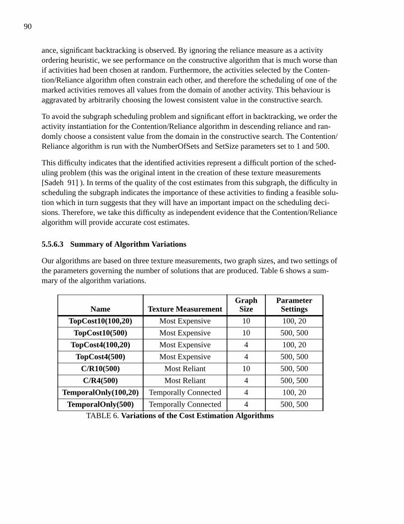
90

ance, significant backtracking is observed. By ignoring the reliance measure as a activityordering heuristic, we see performance on the constructive algorithm that is much worse thanif activities had been chosen at random. Furthermore, the activities selected by the Conten-tion/Reliance algorithm often constrain each other, and therefore the scheduling of one of themarked activities removes all values from the domain of another activity. This behaviour isaggravated by arbitrarily choosing the lowest consistent value in the constructive search.

To avoid the subgraph scheduling problem and significant effort in backtracking, we order theactivity instantiation for the Contention/Reliance algorithm in descending reliance and ran-domly choose a consistent value from the domain in the constructive search. The Contention/Reliance algorithm is run with the NumberOfSets and SetSize parameters set to 1 and 500.

This difficulty indicates that the identified activities represent a difficult portion of the sched-uling problem (this was the original intent in the creation of these texture measurements[Sadeh 91] ). In terms of the quality of the cost estimates from this subgraph, the difficulty inscheduling the subgraph indicates the importance of these activities to finding a feasible solu-tion which in turn suggests that they will have an important impact on the scheduling deci-sions. Therefore, we take this difficulty as independent evidence that the Contention/Reliancealgorithm will provide accurate cost estimates.

5.5.6.3 Summary of Algorithm Variations

Our algorithms are based on three texture measurements, two graph sizes, and two settings ofthe parameters governing the number of solutions that are produced. Table 6 shows a sum-mary of the algorithm variations.

Name Texture MeasurementGraph

SizeParameter

Settings

TopCost10(100,20) Most Expensive 10 100, 20

TopCost10(500) Most Expensive 10 500, 500

TopCost4(100,20) Most Expensive 4 100, 20

TopCost4(500) Most Expensive 4 500, 500

C/R10(500) Most Reliant 10 500, 500

C/R4(500) Most Reliant 4 500, 500

TemporalOnly(100,20) Temporally Connected 4 100, 20

TemporalOnly(500) Temporally Connected 4 500, 500

TABLE 6. Variations of the Cost Estimation Algorithms

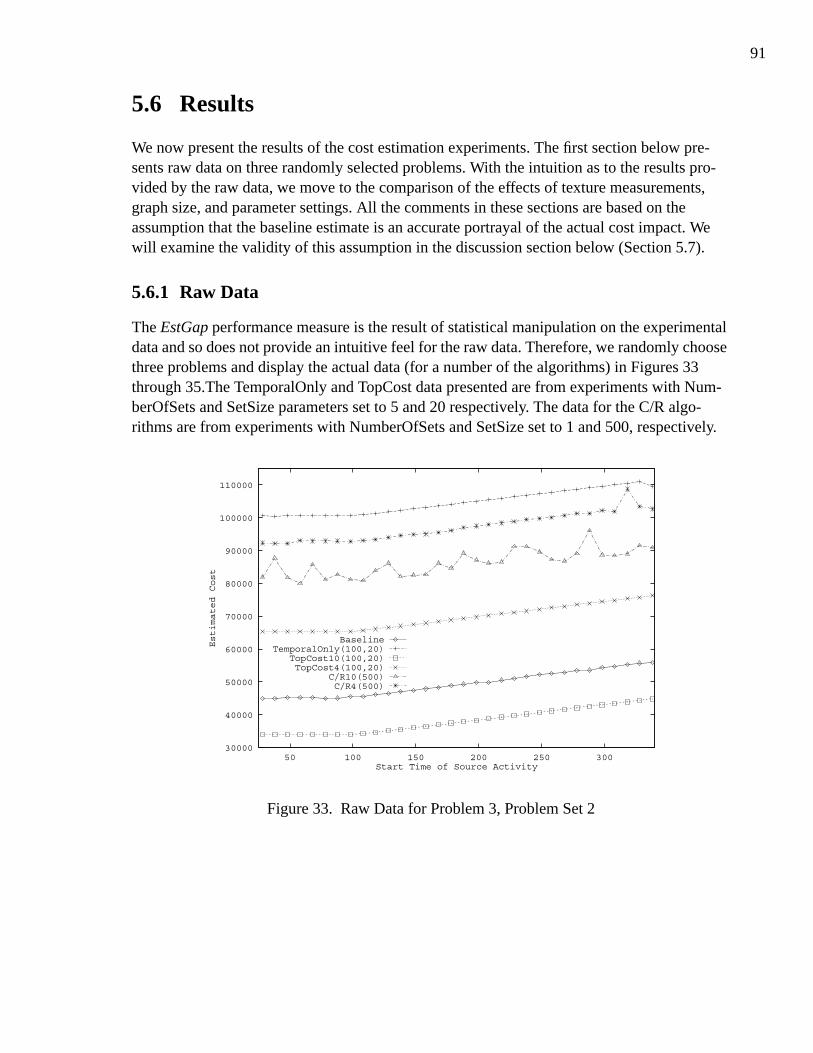
91

5.6 Results

We now present the results of the cost estimation experiments. The first section below pre-sents raw data on three randomly selected problems. With the intuition as to the results pro-vided by the raw data, we move to the comparison of the effects of texture measurements,graph size, and parameter settings. All the comments in these sections are based on theassumption that the baseline estimate is an accurate portrayal of the actual cost impact. Wewill examine the validity of this assumption in the discussion section below (Section 5.7).

5.6.1 Raw Data

The EstGap performance measure is the result of statistical manipulation on the experimentaldata and so does not provide an intuitive feel for the raw data. Therefore, we randomly choosethree problems and display the actual data (for a number of the algorithms) in Figures 33through 35.The TemporalOnly and TopCost data presented are from experiments with Num-berOfSets and SetSize parameters set to 5 and 20 respectively. The data for the C/R algo-rithms are from experiments with NumberOfSets and SetSize set to 1 and 500, respectively.

Figure 33. Raw Data for Problem 3, Problem Set 2

30000

40000

50000

60000

70000

80000

90000

100000

110000

50 100 150 200 250 300

Estimated Cost

Start Time of Source Activity

BaselineTemporalOnly(100,20)

TopCost10(100,20)TopCost4(100,20)

C/R10(500)C/R4(500)

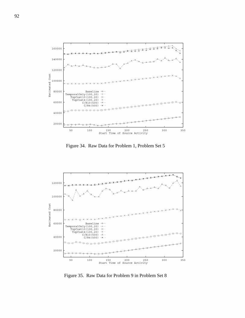
92

Figure 34. Raw Data for Problem 1, Problem Set 5

Figure 35. Raw Data for Problem 9 in Problem Set 8

20000

40000

60000

80000

100000

120000

140000

160000

50 100 150 200 250 300 350

Estimated Cost

Start Time of Source Activity

BaselineTemporalOnly(100,20)

TopCost10(100,20)TopCost4(100,20)

C/R10(500)C/R4(500)

20000

40000

60000

80000

100000

120000

50 100 150 200 250 300 350

Estimated Cost

Start Time of Source Activity

BaselineTemporalOnly(100,20)

TopCost10(100,20)TopCost4(100,20)

C/R10(500)C/R4(500)

93

A number of observations can be made from these data:

• Across all three problems, the TopCost plots seem to be close to a vertical translation of theBaseline plot. This indicates a high quality estimate. The Contention/Reliance plots are, incontrast, bumpy, indicating a less close matching with the baseline estimates

• In Figure 33, we see that the TopCost10 estimation is less than the baseline estimation. Thisoccurs in other problems and in fact, in some problems, the TopCost4 estimations less thanthe baseline estimates. This arises from the fact, that in some cases, the TopCost algorithmsare scheduling more of the non-zero cost activities than the Depth algorithm. This pointcalls into question the accuracy of the baseline estimations (see Section 5.7).

5.6.2 Texture Measurements

To compare the efficacy of the texture measurements we control for both the size of the sub-graph and the settings of the parameters. This requires that we compare the algorithms on sub-graphs of size 4 (the only size that the TemporalOnly algorithm uses) and use parametersettings of 1 and 500 for NumberOfSets and SetSize respectively (the only parameter settingsthat the Contention/Reliance algorithms use). The EstGap results are presented in Figure 36.

Figure 36. The EstGap Statistic for Estimations using Different Texture Measurement

Recall, that the EstGap statistic is a measure of the variation in the difference in estimatesbetween the algorithm and the baseline. Observations:

200

400

600

800

1000

1200

1400

1600

1800

2000

1 2 3 4 5 6 7 8

Average Estimation Gap

Problem Set

TemporalOnly(500)TopCost4(500)

C/R4(500)

94

• TopCost outperforms TemporalOnly which in turn outperforms the Contention/Reliancealgorithm. While we expected that TopCost would produce superior estimates to Temporal-Only, it is surprising that Contention/Reliance algorithm performs so poorly. We will returnto this point in our discussion.

• None of the algorithms perform well. A EstGap of 200 means that the standard deviation inthe differences between the algorithm and the baseline estimates is 200. In other words, theestimations made by even the best algorithm estimates are not a constant difference fromthe baseline. This result contrasts to the raw data given in Figures 33 through 35. There, wenoted that the TopCost algorithms appeared to be a vertical translation of the baseline. Ifthis were the case the EstGap value would be 0. This conflict is an artifact of the scale usedin Figures 33 through 35. The estimation costs are between 2000 and 160000. Given thatscale, estimates with an EstGap measure of 200 does not appear to vary widely.

Figure 37 compares the ChangeActivity count for each of the algorithms. With the parametersettings used, each of algorithm finds a single solution using the backtracking algorithm andthen 499 solutions by randomly changing the start time of one of the scheduled activities.

Figure 37. The ChangeActivity Count Estimations using Different Texture Measurement

Observation:

• We expect that the ChangeActivity count across the algorithms would be the same, sincethey are using the same sized subgraph and the same parameter settings. Figure 37 showsthat this is not the case.

14000

16000

18000

20000

22000

24000

1 2 3 4 5 6 7 8

Average ChangeActivity Count

Problem Set

TemporalOnly(500)TopCost4(500)

C/R4(500)

95

Further analysis reveals that the difference among the algorithms is in the number of assign-ments during the random phase of the algorithm. Normally, the random phase reassigns activ-ities SetSize - 1 times. The only exception is when all the possible values of all the scheduledactivities have been assigned or are inconsistent. The assignment of the source value signifi-cantly prunes the possible values of temporally connected activities. For example, the mini-mum make-span of a particular order is 100 time units, the earliest start time is 0, and theduration of each of the 5 activities is 20. The earliest temporally consistent start time for thefinal activity is 80. The final activity is the source activity and 80 is selected as a candidatevalue. After assigning the final task to 80, the value propagation prunes the domains of theeach of the temporally connected activities to a singleton set. With the TemporalOnly algo-rithm, the temporally connected activities are the activities in the subgraph, therefore there isonly a single consistent solution on the subgraph. Instead of generating 499 solutions, the ran-dom phase does not generate any because there are no consistent values to assign any of theactivities in the subgraph.

This is seen to a lesser extent in the Contention/Reliance algorithm because pruning of valueswhen marked activities are scheduled is lessened because the marked activities are not neces-sarily temporally connected and the Contention/Reliance assigns random values rather thanthe lowest consistent value.

5.6.3 Subgraph Size

The only estimation algorithms where the size of the subgraph is varied are the Contention/Reliance algorithm and the TopCost algorithm.11 The EstGap statistics of both algorithms(with the NumberOfSets and SetSize parameters set at 1 and 500 respectively) are presentedin Figure 38. The effect of the subgraph size on the ChangeActivity count is presented in Fig-ure 39.

Two surprising results arise from the EstGap data in Figure 38:

• TopCost4 is as good as the TopCost10 algorithm on half of the problem sets. This indicatesthat a small subgraph of activities (e.g 4) were largely responsible for determining theimpact of the scheduling decision.

• The Contention/Reliance algorithm on a larger subgraph actually performs worse thanwhen it is executed on a small subgraph. This is unexpected, though it is mirrored in thevariability seen in the C/R10 algorithm in the raw data (see Figures 33-35). We will returnto this point in the discussion section below (see Section 5.7).

Figure 39 reflects the trend of a larger ChangeActivity count for the algorithms with largersubgraphs. This is expected since the size of the subgraph has significant effect of the numberof assignments and, therefore, the number of times that value propagation is done in the con-structive algorithm.

11. Recall that because the TemporalOnly algorithm formed its subgraph only via temporal constraint links, thesize of the subgraph is a constant.

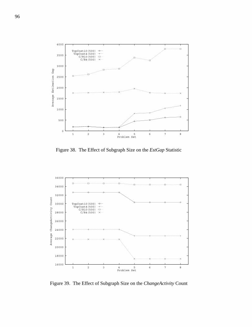
96

Figure 38. The Effect of Subgraph Size on the EstGap Statistic

Figure 39. The Effect of Subgraph Size on the ChangeActivity Count

0

500

1000

1500

2000

2500

3000

3500

4000

1 2 3 4 5 6 7 8

Average Estimation Gap

Problem Set

TopCost10(500)TopCost4(500)

C/R10(500)C/R4(500)

16000

18000

20000

22000

24000

26000

28000

30000

32000

34000

36000

1 2 3 4 5 6 7 8

Average ChangeActivity Count

Problem Set

TopCost10(500)TopCost4(500)

C/R10(500)C/R4(500)

97

5.6.4 Parameter Settings

Two sets of parameter setting were used in the experiments. This first assigned NumberOfSetsand SetSize to 5 and 20, respectively. These settings require that 5 solutions are produced foreach value of the source activity by the backtracking algorithm. For each backtracking solu-tion, 19 random solutions are found. The second set of parameters were 1 and 500 respec-tively for NumberOfSets and SetSize. The latter settings produce a single backtrackingsolution and 499 random solutions are for each value of the source activity.

The results in the EstGap and ChangeActivity measures are presented in Figures 40 and 41.Note that the different parameters, in the graphs, are specified by the SetSize and the totalnumber of solutions. In cases where the two are equal, only one number is displayed.

Observations:

• Figure 40 shows that on 1 bottleneck problems, the different parameter settings have noeffect on the EstGap. The algorithms that find fewer constructive solutions actually per-form better on the problems with 2 bottlenecks than the corresponding algorithms that finda larger number of backtracking solutions.

• The effect on the ChangeActivity count is much as expected: the algorithms that use moreconstructive search (and hence more value propagation) incur a higher ChangeActivitycount.

Figure 40. The Effect of Parameter Settings on the EstGap Statistic

0

200

400

600

800

1000

1200

1400

1600

1800

1 2 3 4 5 6 7 8

Average Estimation Gap

Problem Set

TemporalOnly(100,20)TemporalOnly(500)TopCost10(100,20)

TopCost10(500)TopCost4(100,20)

TopCost4(500)

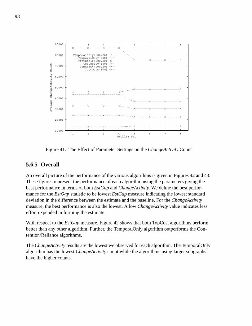
98

Figure 41. The Effect of Parameter Settings on the ChangeActivity Count

5.6.5 Overall

An overall picture of the performance of the various algorithms is given in Figures 42 and 43.These figures represent the performance of each algorithm using the parameters giving thebest performance in terms of both EstGap and ChangeActivity. We define the best perfor-mance for the EstGap statistic to be lowest EstGap measure indicating the lowest standarddeviation in the difference between the estimate and the baseline. For the ChangeActivitymeasure, the best performance is also the lowest. A low ChangeActivity value indicates lesseffort expended in forming the estimate.

With respect to the EstGap measure, Figure 42 shows that both TopCost algorithms performbetter than any other algorithm. Further, the TemporalOnly algorithm outperforms the Con-tention/Reliance algorithms.

The ChangeActivity results are the lowest we observed for each algorithm. The TemporalOnlyalgorithm has the lowest ChangeActivity count while the algorithms using larger subgraphshave the higher counts.

10000

20000

30000

40000

50000

60000

70000

80000

90000

1 2 3 4 5 6 7 8

Average ChangeActivity Count

Problem Set

TemporalOnly(100,20)TemporalOnly(500)TopCost10(100,20)

TopCost10(500)TopCost4(100,20)

TopCost4(500)

99

Figure 42. The Best EstGap Statistic for Each Texture Measurement and Subgraph Size

Figure 43. The Lowest ChangeActivity Counts for Each Texture Measurement and SubgraphSize

0

500

1000

1500

2000

2500

3000

3500

4000

1 2 3 4 5 6 7 8

Average Estimation Gap

Problem Set

TemporalOnly(500)TopCost10(500)TopCost4(500)

C/R10(500)C/R4(500)

10000

15000

20000

25000

30000

35000

1 2 3 4 5 6 7 8

Average ChangeActivity Count

Problem Set

TemporalOnly(500)TopCost10(500)TopCost4(500)

C/R10(500)C/R4(500)

100

5.7 Discussion

In comparing our expectations and the experimental results, we find a number of surprisingand anomalous results. In summary:

1. The raw data shows that on some problems the estimates found by TopCost10 and Top-Cost4 have a lower average cost than the baseline estimate (Figure 33).

2. The poor performance of the Contention/Reliance algorithms is demonstrated both by theEstGap statistic and in the bumpiness of the C/R plots in the raw data (Figures 33-36).

3. The estimates of the TopCost4 algorithm are as good as the TopCost10 estimates on thefirst 4 problem sets (Figure 38).

4. The estimates of the C/R10 algorithm are worse than those found by the C/R4 algorithmacross all problems (Figure 38).

Recall that our expectations were based on the assumption that the baseline estimate was anaccurate reflection of the actual impact of the scheduling decisions. Each of these pointsbrings into question that assumption. We review the Depth algorithm that creates the baselineestimate and then look at each of the above points in turn.

5.7.1 The Depth Algorithm

The Depth algorithm uses a subgraph based on proximity to the source activity. All activitieswithin a specified radius, L, are marked. The baseline estimate is calculated with L = 1. Thestructure of the experimental problems results in a subgraph of about 21 activities. Each ofthese activities is scheduled using the constructive algorithm and the cost of the solution isfound. The cost for the Depth algorithm (as for all algorithms used here) is found by relaxingthe constraints so that the assignments are satisfied. In cases where one or both of the activitiesare not assigned, a worst case estimate (largest cost) based on the remaining possible valuesfor the unassigned activities is used.

It is important to note that the solution on the subgraph is not necessarily a partial schedule forthe entire graph. It may be the case that, due to the assignments of the activities in the sub-graph, no satisfying start time can be found for some activities outside the subgraph. Our costestimates, then, are not necessarily based on partial, globally admissible solutions but ratheron solutions for the subgraph. In general, if we could guarantee that our subgraph solutionswere partial globally admissible solutions, we would be able to solve the whole schedulingproblem. This caveat applies to all algorithms used here, not only the Depth algorithm.

5.7.2 TopCost vs. Baseline

The fact that a texture-based algorithm makes lower estimates than the baseline, indicates thatthere are relaxable constraints for which the Depth algorithm is using an higher estimate thanthe TopCost algorithm. Because we use the worst case estimate for relaxable constraintswhere one or both activities are not assigned, we expect algorithms that perform better analy-

101

sis (i.e. use fewer worst case estimates) will tend to find lower cost estimates. Further, weexpect that the depth of analysis will correspond to the quality of the estimate: the more activ-ities we assign, the more likely that the impact of a scheduling decision on the subgraph willreflect the global impact. Therefore, we expect that the lower estimates correspond to betterquality estimates.

This reasoning must be tempered with the realization that the solutions on the subgraph arenot necessarily partial solutions for the whole graph (see Section 5.3.5). It is possible thatdespite a lower raw cost estimate, the subgraph solutions are not actually part of an overallsolution. We cannot therefore state categorically that a lower raw cost corresponds toincreased accuracy. We believe, however, that this tends to be the case and so the lower rawcosts of the TopCost algorithm in comparison with the baseline is evidence that TopCost out-performs Depth. The assumption of quality for the baseline estimate is, at the least, suspectgiven these results.

5.7.3 Poor Performance of Contention/Reliance

The Contention/Reliance algorithm is specifically designed to find the activities that relyheavily on a resource at a time when there is a high contention for the resource. It is the mostsophisticated texture measurement used here and the most specific to the scheduling domain.Of any of the texture measurements, it gives the most attention to identification of activities onthe basis of resource-related importance. The Contention/Reliance algorithm should providethe best estimate of the inter-order impact. A possible explanation for the poor performance ofthe C/R algorithms is that it is the baseline, rather than the C/R algorithms, that are at fault.

The results showing that the Contention/Reliance algorithm on a larger graph performs worsethan on a smaller graph, further suggest that the baseline estimate is not accurate. If it is cor-rect that the Contention/Reliance algorithm better reflects the impact via resource constraints,expanding the graph should find a better estimate of the inter-order costs. This is not what wefound. A possible explanation is that the baseline is a poor estimate.

5.7.4 TopCost4 vs. TopCost10

By much the same argument used in the previous section, given an accurate baseline estimate,we expect that the TopCost10 algorithm would outperform TopCost4 on all problems. Ourresults show that on the first 4 problem sets, the two algorithms perform about the same, whileon the latter 4 problem sets the TopCost10 algorithm performs better. We take the fact that theTopCost10 algorithm does not perform substantially better (across all problems) than the Top-Cost4 as a further indication that the baseline estimate does not accurately reflect the true situ-ation.

102

5.7.5 Reassessing the Estimations

These results call into question the accuracy of the baseline estimates used in the experiments.It seems likely that the baseline estimate is inaccurate, however due to the complexity of solv-ing the scheduling problem, no simple techniques are available to independently assess thequality of the baseline estimate.

We require an independent comparison of the subgraph identification algorithms. This com-parison can be accomplished if the estimation algorithms are embedded within a completescheduling system. Each of these algorithms can be used as the value ordering heuristic (whileholding the other techniques within the scheduling algorithm constant). The texture measure-ment that more accurately reflects the actual impact will lead to better (e.g. lower cost) sched-ules in less time (due to the lessening of the backtracking effected by a good value ordering).We leave this integration for future work.

5.8 Conclusion

These experiments are the first demonstration, of which we are aware, that the propagation ofcost information in a scheduling problem is not limited solely to temporal constraints.

We see these techniques as occupying a middle ground among the previous work in estimationof the impact of assignments. At one extreme is high-complexity, complete preference propa-gation [Sadeh 89] while at the other is the low-complexity, low-accuracy estimate of marginalcost propagation [Sadeh 91] . Therefore, in addition to introducing cost propagation acrossany types of constraints, this work integrates general heuristics to modulate the complexity ofthe propagation and the accuracy of the estimations. Both the generality of constraint propaga-tion and the ability to integrate heuristics stems from the relaxation schema upon which thesealgorithms are built.

5.8.1 Building Practical Algorithms

Despite the generality of the techniques, the proposed propagation techniques are still imprac-tical for use in a scheduling system. This is primarily due to the complexity of the search andthe dependence on the ability to minimize backtracking. Specifically, to use these propagationmethods in full-fledged scheduling a number of issues must be addressed:

• It is necessary to investigate efficient ways of updating the cost curves as scheduling deci-sions at other activities are made. The re-calculation of the impact of each value with eachscheduling decision is clearly impractical.

• With large scheduling horizons, and therefore large domains for each activity, cost estima-tion for every possible value in the activity may be unnecessary. To minimize the timespent assessing likely values, it is desirable to filter values on the basis of inexpensive, fast,local criteria. In our experiments, we found a cost curve at a granularity of every tenthvalue. We suggested that further cost estimation could focus on values in the vicinity of the

103

lower cost values found by the coarse granularity algorithm. This is one possible approach.Further work is needed to identify and compare texture measurements that can be appliedto such pre-filtering of values.

5.9 Summary

This chapter has presented an application of our relaxation schema to schedule optimization.We represent the sources of cost in a schedule by relaxable constraints and define a number ofalgorithms that estimate the impact of activity start times on the overall schedule. The esti-mates are based on the use of the costs of relaxations at activities within a subgraph as a tex-ture measurement of tightness of constraints on those activities. These costs are propagated tothe source activity where they are summed to form the estimate. The constraint relaxationschema allows propagation to flow over all types of constraints. The subgraph (upon which tobase our impact estimates) can be identified without concern for the types of constraints.

The value impact estimates produced by a number of algorithms are compared to a baselineestimate. Results showed that all algorithms performed relatively poorly with respect tomatching the baseline estimates. The number of anomalous results suggest that the baselineestimate for the impact of scheduling decisions does not accurately reflect the real impact.Further work is required, perhaps within a full scheduling system, to compare the texture mea-surements used to identify the subgraphs.

104

105

Chapter 6 Coordination of MultipleAgents

As noted in Chapter 1, our chief motivation for work in constraint relaxation is its applicationto coordination of multiple agents. We adopt a constraint-based model of a multiagent envi-ronment and present a sketch of a mediated constraint relaxation protocol for coordination.The protocol is demonstrated with the aid of an example from the domain of supply chainmanagement. We conclude with a discussion of the bearing that the work in this dissertationhas on coordination.

6.1 A Theory of Coordination

The study of the coordination has arisen from the recognition that a number of disciplines areconcerned with domains in which autonomous agent work for individual or group goals in ashared environment [Malone 92] . These disciplines include such widespread examples aseconomics, biology, sociology, and computer science. The widely accepted definition forcoordination is the managing of dependencies between activities [Malone 92] .

Within computer science much of the coordination work has been done in Distributed Artifi-cial Intelligence [Distributed 87] [Distributed 89] . Previous work has addressed topics suchas negotiation [Lesser 81] [Davis 83] [Rosenschein 85] [Durfee 87a] [Durfee 91] , dis-tributed planning [Conry 86] [Pope 92] , and the modeling of other agents [Sycara 89][Cohen 91] [Shoham 92] .

We are pursuing the development of a theory of coordination with immediate application tothe area of supply chain management. Our model of coordination rests on the constraint-basedproblem solving model used throughout this dissertation. We view individual agents as con-straint-based problem solvers. The agent interactions, therefore, are the creation, deletion, andexchange of constraints. Agents constrain each other through explicit commitments orthrough operations on the environment which indirectly place constraints on other agents. Anexample, of the former, in the supply chain would be for the manager of the resources to com-mit to the delivery of a raw material to a factory at a certain date. This commitment constrainsthe resource manager to make the delivery of the specified material and constrains the receiv-ing factory in the actions it can take before and after delivery. An example of indirect interac-tion is when two factories use a shared resource pool. Use of the pool by one factory placesconstraints on the action of the other.

106

With this perspective, the environment is characterized by a distributed constraint graphshared among the agents. Coordination is necessary when an agent is unable to meet a com-mitment: the interdependencies between the activities at different agents require management.By failing to meet a commitment, the agent creates an infeasible constraint graph. Coordina-tion is a reconfiguration of the graph, possibly including constraint relaxation, in order to re-establish feasibility.

6.2 A Mediated Approach to Coordination

In contrast to the negotiated approach taken by others (e.g. [Lesser 81] [Durfee 87a] [Durfee87b] [Durfee 91] ), we adopt a mediated approach to coordination. We identify a specialagent, the mediator,1 that has coordination knowledge and is responsible for re-establishingfeasibility in the shared constraint graph.

6.2.1 The Role of the Mediator

When an event occurs that prevents an agent from meeting a constraint, the mediator will benotified. The mediator then builds an augmented constraint graph that represents, at somelevel of abstraction, the distributed constraint graph. This graph is built with information thatthe mediator has locally and from information gathered from other agents. The communicatedinformation will typically be local constraints and relaxation costs that have an impact on thesituation but are not yet represented in the augmented constraint graph. There is no need torepresent the same level of detail in all parts of the graph. The mediator can represent impor-tant subgraphs to arbitrary detail by engaging in a dialogue with the relevant agents about con-straints and the costs of various relaxations.

Once the augmented graph is formed, the mediator uses constraint relaxation to evaluate alter-natives. It is likely that the forming of the constraint graph will be interleaved by evaluationsof alternatives. The relaxation algorithm may identify a subgraph where more detail isrequired. The mediator can then engage in further dialogue with the relevant agents to flesh-out the appropriate areas of the graph. Once an acceptable solution has been found, the media-tor makes suggestions to the agents involved as to the relaxations that will most efficiently re-establish feasibility.

6.2.2 Why Mediation?

Our adoption of a mediated approach is a starting point in our exploration of coordination. Weintend to move toward more distributed methods base on inter-agent negotiation. There are anumber of good reasons to adopt mediation, especially with our domain of application.

• Mediation minimizes the coordination knowledge required by each agent.

1. The agent may also have other functional abilities and responsibilities that are unconnected with meditation.

107

• The supply chain domain is highly-structured and only requires explicit coordination tech-niques when unexpected events occur.

• The constraint graph upon which relaxation needs to be performed is partially representedin the existing schedule or plan. The agent originally responsible for the scheduling orplanning is a natural choice as a mediator.

• Coordination in the supply chain is necessary when the schedule is found to be infeasible.Scheduling difficulties can often be traced to a particular scarce resource [Smith 89] [Fox90] [Sadeh 91] . The work of [Sathi 89] indicates that problems with such keystone ele-ments can be solved better by mediated protocols.

We now illustrate our approach to coordination with a scenario from the supply chain.

6.3 Supply Chain Management Revisited

Recall that, in a manufacturing enterprise, the supply chain consists of all activities leading tothe delivery of a product to a customer (e.g. marketing, material planning, production plan-ning, production control, transportation, customer service). There are a number of agentswithin the supply chain that are responsible for these various activities.

At the logistics level, we view each factory within the enterprise as a resource, able to performa number of activities. The activities produce a quantity of a particular resource over sometime period and logistics-level scheduling assigns factories to produce specific quantities ofresources at particular times. Factories commit to the high-level schedule and schedule theintra-factory activities to meet the commitment. As long as the operations of the enterprise donot violate the assumptions and aggregate information upon which commitments are based,no explicit coordination is necessary. When an unexpected event occurs such that an agent cannot meet an existing constraint, the agents must coordinate their efforts to respond optimally.

6.3.1 An Example

In Chapter 1, we used a requested order change as an example of an unexpected, conflict-causing event. Here we present an instantiation of a supply chain simulation and show theactions taken by each agent in reaction to this event.

We use the following agents in our example:

• Logistics: responsible for the logistics-level scheduling.• Order Acquisition (OA): responsible for all order-related contact with customers includ-

ing order entry, cancellation, and modification.• Resource Manager (RM): responsible for managing consumable resources (e.g. timely

ordering of raw materials) and usable resources (e.g. scheduling of regular maintenance).• Factory Agents (F1, …, F5): each of the five factories is represented, at the logistics level,

by a single agent (typically the factory-level scheduler).

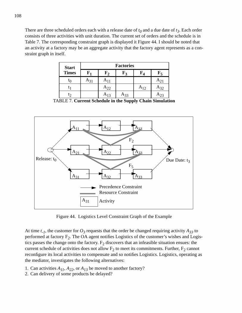
108

There are three scheduled orders each with a release date of t0 and a due date of t3. Each orderconsists of three activities with unit duration. The current set of orders and the schedule is inTable 7. The corresponding constraint graph is displayed it Figure 44. I should be noted thatan activity at a factory may be an aggregate activity that the factory agent represents as a con-straint graph in itself.

Figure 44. Logistics Level Constraint Graph of the Example

At time t-1, the customer for O3 requests that the order be changed requiring activity A33 toperformed at factory F2. The OA agent notifies Logistics of the customer’s wishes and Logis-tics passes the change onto the factory. F2 discovers that an infeasible situation ensues: thecurrent schedule of activities does not allow F2 to meet its commitments. Further, F2 cannotreconfigure its local activities to compensate and so notifies Logistics. Logistics, operating asthe mediator, investigates the following alternatives:

1. Can activities A11, A22, or A13 be moved to another factory?2. Can delivery of some products be delayed?

StartTimes

Factories

F1 F2 F3 F4 F5

t0 A31 A11 A21

t1 A22 A12 A32

t2 A13 A33 A23

TABLE 7. Current Schedule in the Supply Chain Simulation

Release: t0F5

A11

Due Date: t3

F2

A31

Precedence ConstraintResource Constraint

Activity

A12 A13

A21 A22 A23

A31 A32 A33

109

In order to answer these questions, the mediator must request information from other agents.A representation of the communication that takes place for option 1 is as follows:

• Logistics to RM: “What factories can be perform activities A11, A22 and A13?”• RM to Logistics: “F4, but quality will decrease.”2

• Logistics to OA: “What is the cost, due to relations with the customer, of the reduced qual-ity on O2 and O1?”

• OA to Logistics: “3 each.”

For option 2, Logistics must know the cost of late delivery of each order:

• Logistics to OA: “What is the cost of late delivery on each order?”• OA to Logistics: “O1: 5 per time unit, latest acceptable delivery is t6.”• OA to Logistics: “O2: 5 per time unit, latest acceptable delivery is t6.”• OA to Logistics: “O3: 2 per time unit, latest acceptable delivery is t6.”

This information from other agents allows the mediator to build the augmented constraintgraph upon which a relaxation algorithm can then run. The algorithm will not necessarilychoose one of the options, but rather it will investigate possibilities of a combination of mov-ing some activities and of delaying delivery of some products.

In the example, the least expensive solution is to move A13 to F4 and A33 to F2 at a cost of 3.The schedule after relaxation is shown in Table 8. The corresponding constraint graph is dis-played it Figure 45. Note the change in the resource constraints due to the relaxation.

2. Work is progressing on a theory of quality that will make such a response meaningful [Kim 94] .

StartTimes

Factories

F1 F2 F3 F4 F5

t0 A31 A11 A21

t1 A22 A12 A32

t2 A33 A13 A23

TABLE 8. Schedule After Relaxation

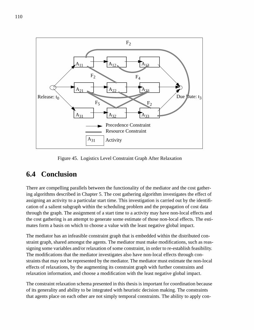
110

Figure 45. Logistics Level Constraint Graph After Relaxation

6.4 Conclusion

There are compelling parallels between the functionality of the mediator and the cost gather-ing algorithms described in Chapter 5. The cost gathering algorithm investigates the effect ofassigning an activity to a particular start time. This investigation is carried out by the identifi-cation of a salient subgraph within the scheduling problem and the propagation of cost datathrough the graph. The assignment of a start time to a activity may have non-local effects andthe cost gathering is an attempt to generate some estimate of those non-local effects. The esti-mates form a basis on which to choose a value with the least negative global impact.

The mediator has an infeasible constraint graph that is embedded within the distributed con-straint graph, shared amongst the agents. The mediator must make modifications, such as reas-signing some variables and/or relaxation of some constraint, in order to re-establish feasibility.The modifications that the mediator investigates also have non-local effects through con-straints that may not be represented by the mediator. The mediator must estimate the non-localeffects of relaxations, by the augmenting its constraint graph with further constraints andrelaxation information, and choose a modification with the least negative global impact.

The constraint relaxation schema presented in this thesis is important for coordination becauseof its generality and ability to be integrated with heuristic decision making. The constraintsthat agents place on each other are not simply temporal constraints. The ability to apply con-

Release: t0F5

A11

Due Date: t3

F4

A31

Precedence ConstraintResource Constraint

Activity

A12 A13

A21 A22 A23

A31 A32 A33

F2

F2

F2

111

straint relaxation across all constraint types is a requirement for assessment of the relaxationdecisions. Furthermore, there is no central representation of the constraint graph and, in anynon-trivial agent environment, the graph will be too large to operate on directly. The ability tomodulate search by heuristic decision making is a necessity even on the partial graph gener-ated by the mediator.

112

113

Chapter 7 Concluding Remarks

7.1 Contributions

This thesis makes contributions in five areas:

• A generalization of the constraint model allowing representation of the semantic content ofconstraint relaxations.

• A flexible, general relaxation schema within which algorithms can be specified.• A specification of three relaxation algorithms useful in small Partial Constraint Satisfaction

Problems (PCSPs), constraint relaxation, and constraint satisfaction problems.• Application of the propagation techniques and texture-based heuristics within the relax-

ation schema to schedule optimization.• The modeling of multiagent coordination as a problem requiring constraint relaxation.

The final point was discussed in the previous chapter. We address the first four areas in turn.

7.1.1 A Generalized Constraint Model

The constraint model that we introduce uses a generator function at each constraint to producealternative constraints and a cost function assessing the local impact of a constraint relaxation.This allows for very general approach to problem specification and the explicit use of relax-ation generators as operators in constraint-directed search. The modification to the constraintmodel is a true generalization because it allows the use of either constraint satisfaction or con-straint relaxation search techniques.

Our model expands the semantics of constraint relaxation because of the ability to assess thelocal cost of a specific relaxation. The impact of a relaxation depends not only on the originalconstraint, but also on the relaxation that is done. Simply ignoring a constraint has a very dif-ferent effect than expanding the set of satisfying tuples by one entry. Previous work has failedto address this difference. The ability to represent and reason about the differential impact ofmodifications to problem constraints is a foundational requirement of any theory of constraintrelaxation and of any relaxation-based search technique.

114

7.1.2 A Schema for Relaxation Algorithms

A schema for relaxation algorithms based on the propagation of various types of informationbetween variables is presented. The schema defines a class of algorithms with varying com-plexity and performance characteristics. The specification of procedures used at five heuristicdecision points is required:

1. Selection of the source variable from where propagation originates.2. Selection of a set of candidate values for each variable.3. Selection of a set of outgoing constraints from each variable.4. Selection of a set of candidate constraints at each outgoing constraint.5. Selection of the value-commitment at the source variable.

The schema allows these heuristic choices to be tailored to certain constraint types or specificrun time conditions. By isolating the heuristics of an algorithm at a few key points, the schemaallows for specification of a variety of algorithms of different complexity and performance. Ifalgorithms are categorized by their complexity and performance characteristics, it may bepossible to make the choice of algorithm at run time based on structural problem properties,time pressure, required solution quality, and other factors.

The central contributions of the relaxation schema are its generality and its ability to be inte-grated with arbitrarily complex heuristics. The generality allows the gathering of relaxationinformation across all types of constraints. This is demonstrated in Chapters 4 and 5, wherewe define algorithms based on the schema for PCSP graphs and schedule optimization graphsrespectively. The integration of heuristics becomes extremely important when the size of thegraphs is non-trivial. The results of the exponential algorithms for the PCSPs demonstrate thatwithout heuristic decision making, graphs of 16 or more nodes are intractable.

7.1.3 Three Relaxation Algorithms for PCSPs

Using the relaxation schema, we specify three relaxation algorithms with the performance/complexity trade-off in mind: SMV, MMV, and MC. The latter algorithm is a variation of theMinConflicts repair algorithm [Minton 92] . Experiments compare performance against thepartial extended forward checking algorithm, judged by [Freuder 92] to be the best PCSPalgorithm investigated. Results showed that in almost all cases the SMV and MMV algo-rithms performed significantly fewer constraint checks than the PCSP algorithm while thequality of the solutions was close to optimal.

PCSPs are a special case of constraint relaxation, and, as such, they do not address the seman-tic issues that are focal in our constraint model. For this reason, we do not view the work onPCSPs in itself as having a large impact on constraint relaxation. We use PCSPs here as anexample of the applicability and generality of the relaxation schema. More important is theindication, from the number of consistency checks, that the experimental problems are

115

approximately at the limit of size to which both the relaxation and complete algorithms can beapplied. This underscores the requirement, noted above, for heuristic decision making in prob-lems of non-trivial size.

7.1.4 Application of the Relaxation Schema to Schedule Optimization

We use the value and cost propagation of the relaxation schema to estimate the impact ofassigning an activity to a start time in a schedule optimization domain. Our experiments tocompare the quality of cost estimate produced by algorithms using three texture measure-ments were inconclusive due to the inability to find an accurate baseline estimate for theactual cost impact of scheduling decisions. We suggest that these estimation algorithmsshould be compared by integration of each algorithm within a larger scheduling system. Thequality of the schedules and the time performance of the overall scheduler will then indicatethe relative merits of the cost estimation algorithms.

Despite the lack of conclusive results, the texture measure-based algorithms represent the firstexample, of which we are aware, of the ability to dynamically choose a subgraph for cost esti-mation, independent of constraint type. We believe this ability is advantageous for two rea-sons:

1. The dynamic identification of the subgraph allows the modification of the basis for sched-uling decisions as the schedule evolves. Furthermore, the size of the subgraph and depth ofanalysis on the subgraph can be tailored to both the quality and processing time require-ments of the particular scheduling situations.

2. Texture measurements are a prime technique for the identification of this subgraph. Usingdynamically calculated texture measurements as a basis for heuristic decisions can achievesignificant algorithmic savings by limiting the size of the data set which must be searchedover. These savings can come at little penalty to performance.

Our inability to form an accurate baseline estimate against which we could compare the algo-rithms, prevents us, in the work done here, from assessing either of these points.

7.2 Future Work

A described in Chapter 6, the main body of our future work will be in the application of con-straint relaxation and the techniques developed here to coordination of multiple agents in ashared environment. Nevertheless, there are a number of other areas where interesting futureresearch may be pursued. Four broad areas for future research are:

1. The characterization of the trade-offs made by relaxation algorithms. The relaxationalgorithms are heuristic-based algorithms that are not guaranteed to find the optimal solu-tion to problems. There is a classic trade-off of processing time for quality of solution.Given that this trade-off is made, it is necessary to characterize the types of solutions that

116

will not be found by algorithms defined within the relaxation schema. Such a characteriza-tion would allow the selection of algorithms based on the dynamic factors (e.g. time pres-sure, quality of solution desired by the user) surrounding a particular problem instance.

2. The continued investigation of texture measurements as a basis for heuristic deci-sions. The constraint research has, to this point, shown that exponential algorithms canonly be avoided in very specific conditions. These conditions are rare in real problems andthe effort required to create these conditions can be prohibitive. We require algorithms thatmake use of well-founded heuristic decisions to eliminate large portions of the searchrequired to find a solution. Texture measurements provide this foundation.

3. The exposition and investigation of relaxation as a general search technique. We char-acterize relaxation throughout this thesis as changing the definition of a constraint. Webelieve that this can be used as a powerful general search technique that is complementaryto constraint satisfaction search techniques.

4. The application of the relaxation techniques to scheduling. In characterizing the sourceof costs in a schedule as relaxable constraints, we achieve an increase in the scope of opti-mization criteria that can be expressed. In the scheduling domain, little work has been doneon problems where a large number of constraints can be relaxed. Furthermore, research isalso required on the efficient use of the general propagation techniques proposed on thisdissertation. We believe that scheduling algorithms using such a technique will realize asignificant increase in the quality of schedules produced.

7.3 Summary

Constraint relaxation is a general search method on any problem that can be expressed in theconstraint paradigm. We have shown that a key its use is the recognition of the semanticnature of relaxation: the meaning of a constraint relaxation is embedded in the original mean-ing of the constraint and in the way in which the relaxation modifies the constraint.

We have presented a general algorithm schema for relaxation algorithms and shown its appli-cability to general constraint problems and schedule optimization. Future work will examinethe application and further development of relaxation techniques in the area of multiagentcoordination.

117

Bibliography

[Allen 83] Allen, J.F. Maintaining Knowledge about Temporal Intervals. Communicationsof the ACM. 26 (11):832-843, November, 1983.

[Bakker 93] Bakker, R.R., Dikker, F., Tempelman, F., and Wognum, P.M. Diagnosing andSolving Over-determined Constraint Satisfaction Problems. Proceedings ofIJCAI-93. 1993.

[Bazaraa 90] Bazaraa, M.S., Jarvis, J.J., and Sherali, H.D. Linear Programming and NetworkFlows. John Wiley & Sons, Inc., New York, 1990.

[Borning 87] Borning, A., Duisberg, R., Freeman-Benson, B., Kramer, A., and Woolf, M.Constraint Hierarchies. Proceedings of the 1987 ACM Conference on Object-Oriented Programming Systems, Languages and Applications. 1987.

[Borning 88] Borning, A., Maher, M., Martindale, A., and Wilson, M. Constraint Hierarchiesand Logic Programming. Technical Report 88-11-10, Computer Science De-partment, University of Washington, November, 1988.

[Cohen 91] Cohen, P.R. and Levesque, H.J. Teamwork. Nous 35. 1991.

[Conry 91] Conry, S.E., Kuwabara, K., and Lesser, V.R. Multistage Negotiation for Distrib-uted Constraint Satisfaction. IEEE Transactions on Systems, Man, and Cyber-netics. SMC-21 (6):1462-1477, 1991.

[Conry 86] Conry, S.E., Meyer, R.A., Lesser, V.R. Multistage Negotiation in DistributedPlanning. Technical Report 86-67, Department of Computer and InformationScience, University of Massachusetts, December, 1986.

[Cooper 92] Cooper, M. Visual Occlusion and the Interpretation of Ambiguous Pictures. El-lis Horwood, Limited, Chichester, West Sussex, England, 1992.

[Cplex 92] CPLEX. Using the CPLEX Callable Library and CPLEX Mixed Integer LibraryCPLEX Optimization, Inc., 1992.

[Davis 94] Davis, E.D. ODO: A Constraint-Based Scheduler Founded on a UNified Prob-lem Solving Model. Technical Report TR-EIL-94-1, Enterprise Integration Lab-oratories, Department of Industrial Engineering, University of Toronto, 1994.

[Davis 83] Davis, R. and Smith, R.G. Negotiation as a Metaphor for Distributed ProblemSolving. Artificial Intelligence. 20 (1):63-109, 1983.

[Dechter 88] Dechter, R. and Pearl, J. Network-Based Heuristics for Constraint-SatisfactionProblems. Artificial Intelligence. 34 1-38, 1988.

118

[Dechter 89] Dechter, R. and Pearl, J. Tree Clustering for Constraint Networks. Artificial In-telligence. 38 353-366, 1989.

[Dechter 90] Dechter, R., Dechter, A., and Pearl, J. Optimization in Constraint Networks. In-fluence Diagrams, Belief Nets, and Decision Analysis. In Oliver, R.M. andSmith, J.Q., John Wiley and Sons, Ltd, Chicester, England, 1990.

[Descotte 85] Descotte, Y. and Latombe, J.C. Making Compromises among Antagonist Con-straints in a Planner. Artificial Intelligence. 27 183-217, 1985.

[Distributed 87] Huhns, M.N. (editor). Volume 1 Distributed Artificial Intelligence. Pitman Pub-lishing & Morgan Kaufmann Publishers, Los Altos, CA, 1987.

[Distributed 89] Gasser, L. and Huhns, M.N. (editor). Volume 2 Distributed Artificial Intelli-gence. Pitman Publishing & Morgan Kaufmann Publishers, San Mateo, CA,1989.

[Dorn 92] Dorn, J., Slany, W., and Stary, C. Uncertainty Management by Relaxation ofConflicting Constraints in Production Process Scheduling. Working NotesAAAI Spring Symposium on Practical Approaches to Scheduling and Plan-ning. 1992.

[Dubois 93] Dubois, D., Fargier, H., and Prade, H. The Use of Fuzzy Constraints in Job-Shop Scheduling. Working Notes of the IJCAI-93 Workshop on Knowledge-Based Production Planning, Scheduling, and Control. 1993.

[Durfee 87a] Durfee, E.H. and Lesser, V.R. Using Partial Global Plans to Coordinate Distrib-uted Problem Solvers. Proceedings of IJCAI-87, pages 875-883. 1987.

[Durfee 87b] Durfee, E.H., Lesser, V.R., and Corkill, D.D. Cooperation Through Communi-cation in a Distributed Problem Solving Network. Volume 1. Distributed Arti-ficial Intelligence. In Huhns, M.N., Pitman Publishing & Morgan KaufmannPublishers, 1987, pages 29-58, Chapter 2.

[Durfee 91] Durfee, E.H. and Montgomery, T.A. Coordination as Distributed Search in a Hi-erarchical Behavior Space. IEEE Transactions on Systems, Man, and Cyber-netics. SMC-21 (6):1361-1378, 1991.

[Fox 86] Fox, M.S. Observations on the Role of Constraints in Problem Solving. Pro-ceedings of the Sixth Canadian Conference on Artificial Intelligence. 1986.

[Fox 87] Fox, M.S. Constraint-Directed Search: A Case Study of Job-Shop Scheduling.Morgan Kaufman Publishers, Inc., 1987.

[Fox 89] Fox, M.S., Sadeh, N., and Baykan, C. Constrained Heuristic Search. Proceed-ings of IJCAI-89. 1989.

[Fox 90a] Fox, M.S. and Sadeh, N. Why Is Scheduling Difficult? A CSP Perspective. Pro-ceedings of the Ninth European Conference on Artificial Intelligence. 1990.

[Fox 90b] Fox, M.S. Constraint-Guided Scheduling - A Short History of Research atCMU. Computers in Industry. 14 79-88, 1990.

[Fox 92] Fox, M.S. Integrated Supply Chain Management. Technical Report, EnterpriseIntegration Laboratories, Department of Industrial Engineering, University ofToronto, April, 1992.

119

[Freuder 89] Freuder, E. Partial Constraint Satisfaction. Proceedings of IJCAI-89. 1989.

[Freuder 92] Freuder, E. and Wallace, R. Partial Constraint Satisfaction. Artificial Intelli-gence. 58 21-70, 1992.

[Freuder 85] Freuder, E. A Sufficient Condition for Backtrack Bounded Search. Journal ofthe ACM. 32 (4):755-761, 1985.

[Garey 79] Garey, M.R. Computers and Intractability. W.H. Freeman and Company, SanFrancisco, 1979.

[Gaschnig 77] Gaschnig, J. A General Backtrack Algorithm that Eliminates Most RedundantTests. Proceedings of IJCAI-77. 1977.

[Gaschnig 78] Gaschnig, J. Experimental Case Studies of Backtrack vs. Waltz-type vs. NewAlgorithms for Satisficing Assignment Problems. Proceedings of the SecondNational Conference of the Canadian Society for Computational Studies of In-telligence. 1978.

[Ghedira 94] Ghedira, K. Partial Constraint Satisfaction with Multi-Agent Systems Com-bined with Simulated Annealing Process. Proceedings of 14th InternationalConference on Artificial Intelligence, Expert Systems, and Natural Language,Avignon-94. 1994.

[Gruninger 94] Gruninger, M., and Fox, M.S. Proceedings of Second International ConferenceOn Cooperative Information Systems. 1994. To Appear.

[Haralick 80] Haralick, R. and Elliott, G. Increasing Tree Search Efficiency for ConstraintSatisfaction Problems. Artificial Intelligence. 14 263-313, 1980.

[Hillier 80] Hillier, F.S. and Lieberman, G.J. Introduction to Operations Research. Holden-Day, Inc., San Francisco, 1980.

[Huhns 91] Huhns, M.N. and Bridgeland, D.M. Multiagent Truth Maintenance. IEEETransactions on Systems, Man, and Cybernetics. SMC-21 (6):1437-1445, No-vember/December, 1991.

[Ijcai 93] Sadeh, N. (editor). IJCAI-93 Workshop on Knowledge-Based Production Plan-ning, Scheduling, and Control., 1993.

[Interrante 93] Interrante, L.D. and Rochowiak, D.M. A Distributed Agent Architecture for In-tegrating AI and OR in the Dynamic Scheduling of Manufacturing Systems.Working Notes of the IJCAI-93 Workshop on Knowledge-Based ProductionPlanning, Scheduling, and Control. 1993.

[Johnston 92] Johnston, M.D. Spike: AI Scheduling for Hubble Space Telescope After 18Months of Orbital Operations. Working Notes AAAI Spring Symposium onPractical Approaches to Scheduling and Planning. 1992.

[Kim 94] Kim, H.K. and Fox, M.S. Formal Models of Quality and ISO 9000 Compliance:An Information Systems Approach. 48th Annual Quality Congress of theAmerican Society of Quality Control, pages 17-23. 1994.

[Kirkpatrick 83] Kirkpatrick, S., Gelarr, Jr., C.D., and Vecchi, M.P. Optimization by SimulatedAnnealing. Science. 220 (4598):671-680, May, 1983.

[Kumar 92] Kumar, V. Algorithms for Constraint Satisfaction Problems: A Survey. AI Mag-azine. 13 (1):32-44, 1992.

120

[Lansky 88] Lansky, A.L. Localized Event-Based Reasoning for Multiagent Domains. Com-putational Intelligence. 4 319-340, 1988.

[Lesser 81] Lesser, V.R and Corkill, D.D. Functionally Accurate, Cooperative DistributedSystems. IEEE Transactions on Systems, Man, and Cybernetics. SMC-11(1):81-96, January, 1981.

[Lowry 92] Lowry, M. Integration of AI and OR Technologies: Issues and Tradeoffs. Work-ing Notes AAAI Workshop on Production Planning, Scheduling, and Control.1992.

[Mackworth 77] Mackworth, A. Consistency in Networks of Relations. Artificial Intelligence. 899-118, 1977.

[Malone 92] Malone T.W., and Crowston, K. The Interdisciplinary Study of Coordination.Technical Report, Center for Coordination Science, Massachusetts Institute ofTechnology, December, 1992.

[Mcmahon 92] McMahon, M.B. and Dean, J. A Simulated Annealing Approach to ScheduleOptimization for the SES Facility. Working Notes AAAI Spring Symposium onPractical Approaches to Scheduling and Planning. 1992.

[Minton 92] Minton, S., Johnston, M., Philips, A., and Laird, P. Minimizing Conflicts: AHeuristic Repair Method for Constraint Satisfaction and Scheduling Problems.Artificial Intelligence. 58 161-205, 1992.

[Mittal 90] Mittal, S. and Falkenhainer, B. Dynamic Constraint Satisfaction Problem. Pro-ceedings of AAAI-90. 1990.

[Morton 86] Morton, T.E., Lawrence, S.R., Rajoagopalan, S., and Kekre, S. MRP-STAR:PATRIARCH's Planning Module. Technical Report, Graduate School of In-dustrial Administration, Carnegie Mellon University, December, 1986.

[Nadel 88] Nadel, B.A. Tree Search and Arc Consistency in Constraint Satisfaction Algo-rithms. Search in Artificial Intelligence. In L. Kanal and V. Kumar, Springer-Verlag, New York, 1988.

[Nagel 91] Nagel, R.N. et al. 21st Century Manufacturing Enterprise Strategy: An Indus-try Led View. Technical Report, Iacocca Institute, Lehigh University, Bethle-hem PA, 1991.

[Navinchandra 87] Navinchandra, D. and Marks, D.H. Design Exploration Through Constraint Re-laxation. Expert Systems in Computer-Aided Design. In J. Gero, Elsevier Sci-ence Publishers B.V., 1987.

[Navinchandra 91] Navinchandra, D. Exploration and Innovation in Design. Springer-Verlag,New York, 1991.

[Nuitjen 93] Nuitjen, W.P.M., Aarts, E.H.L., van Erp Taalman Kip, D.A.A., and van Hee,K.M. Randomized Constraint Satisfaction for Job-Shop Scheduling. WorkingNotes of the IJCAI-93 Workshop on Knowledge-Based Production Planning,Scheduling, and Control. 1993.

[Page 91] Page, C.D. Jr. and Frisch, A.M. Generalizing Atoms in Constraint Logic. Pro-ceedings of the Second International Conference on Principles of KnowledgeRepresentation and Reasoning. 1991.

121

[Phillips 76] Phillips, D.T., Ravindran, A., and Solberg, J.J. Operations Research. John Wiley& Sons, Inc., New York, 1976.

[Pope 92] Pope, R.P., Conry, S.E., and Meyer, R.A. Distributing the Planning Process in aDynamic Environment. Working Papers of the 11th International Workshop onDistributed Artificial Intelligence. 1992.

[Ravindran 87] Ravindran, A., Phillips, D.T., and Solberg, J.J. Operations Research Principlesand Practice. John Wiley & Sons, Inc., New York, 1987.

[Rosenfeld 76] Rosenfeld, A., Hummel, R.A., and Zucker, S.W. Scene Labeling by RelaxationOperations. IEEE Transactions on Systems, Man, and Cybernetics. 6 1976.

[Rosenschein 85] Rosenschein, J.S. and Genesereth, M.R. Deals Among Rational Agents. Pro-ceedings of IJCAI-85, pages 91-99. 1985.

[Sadeh 89] Sadeh, N. and Fox, M.S. Preference Propagation in Temporal/Capacity Con-straint Graphs. Technical Report CMU-RI-TR-89-2, The Robotics Institute,Carnegie Mellon University, January, 1989.

[Sadeh 91] Sadeh, N. Lookahead Techniques for Micro-Opportunistic Job Shop Schedul-ing. PhD thesis, Carnegie Mellon University, 1991. CMU-CS-91-102.

[Sadeh 94] Sadeh, N. Micro-Opportunistic Scheduling: The MICRO-BOSS FactoryScheduler. Technical Report, The Robotics Institute, Carnegie Mellon Univer-sity, 1994.

[Sathi 89] Sathi, A. and Fox, M.S. Constraint-Directed Negotiation of Resource Realloca-tions. Volume 2. Distributed Artificial Intelligence. In Michael N. Huhns andLes Gasser, Pitman Publishing & Morgan Kaufmann Publishers, 1989, pages163-193, Chapter 8.

[Selman 92] Selman, B., Levesque, H., and Mitchell, D. A New Method for Solving HardSatisfiability Problems. Proceedings of AAAI-92. 1992.

[Shapiro 81] Shapiro, L.G. and Haralick, R.M. Structural Descriptions and Inexact Match-ing. IEEE Transactions on Pattern Analysis and Machine Intelligence. 3(11):504-519, September, 1981.

[Shoham 92] Shoham, Y. and Tennenholtz, M. On the Synthesis of Useful Social Laws forArtificial Agent Societies. Proceedings of the National Conference on ArtificialIntelligence, pages 276-281. 1992.

[Smith 89] Smith, S.F., Ow, P.S., Matthys, D.C., and Potvin, J.Y. OPIS: An OpportunisticFactory Scheduling System. Proceedings of International Symposium for Com-puter Scientists. 1989.

[Stallman 77] Stallman, R.M. and Sussman G.J. Forward Reasoning and Dependency-Direct-ed Backtracking in a System for Computer-Aided Circuit Analysis. Artificial In-telligence. 9 135-196, 1977.

[Sycara 89] Sycara, K.P. Argumentation: Planning Other Agents' Plans. Proceedings ofIJCAI-89, pages 517-523. 1989.

[Van 89] Van Hentenryck, P. Constraint Satisfaction in Logic Programming. MIT Press,1989.

122

[Waltz 75] Waltz, D. Understanding Line Drawings of Scenes with Shadows. The Psychol-ogy of Computer Vision. In P. Winston, McGraw-Hill, 1975.

[Yokoo 92a] Yokoo, M. and Durfee, E.H. Distributed Search Formalisms for DistributedProblem Solving: Overview. Proceedings of the 11th International Workshopon Distributed Artificial Intelligence. 1992.

[Yokoo 92b] Yokoo, M., Durfee, E.H., Ishida, T., and Kuwabara, K. Distributed ConstraintSatisfaction for Formalizing Distributed Problem Solving. Proceedings of the12th International Conference on Distributed Computing Systems. 1992.

[Yokoo 93] Yokoo, M. Constraint Relaxation in Distributed Constraint Satisfaction Prob-lems. Proceedings of the 5th International Conference on Tools with ArtificialIntelligence. 1993.

[Zweben 92] Zweben, M., Davis, E., Daun, B., and Deale, M. Rescheduling with Iterative Re-pair. Technical Report FIA-92-15, Artificial Intelligence Research Branch,NASA Ames Research Center, April, 1992.

[Zweben 94] Zweben, M., Davis, E., Daun, B., and Deale, M. Iterative Repair for Schedulingand Rescheduling. IEEE Transactions on Systems, Man, and Cybernetics.1994. To Appear.