A Scalable Pricing Model for Bandwidth Allocation

A Scalable Pricing Model for Bandwidth Allocation

Adel S. Elmaghraby1 [email protected] 1-(502)-852-0407

Anup Kumar

[email protected]

Mehmed M. Kantardžic [email protected]

Mostafa Gamal Mostafa [email protected]

Computer Engineering and Computer Science Department

Speed Scientific School University of Louisville, KY 40292

1 Contact Person: Adel S. Elmaghraby, CECS Dept., 123 J.B. Speed Bldg., U of L, Louisville, KY, 40292 Phone: 502-852-6304 Fax: 502-852-4713

Abstract

In this paper, we present a scalable pricing model for dynamic bandwidth allocation

combined with simulation scenarios that demonstrate different aspects of a scalable service

delivery model and at the same time guarantees a good level of resource utilization. The model

allows for increasing the revenue while maintaining an acceptable level of quality of service

(QoS) for users. Simulation results of our model show that selecting an appropriate bandwidth

allocation policy can reduce the number of blocked users, achieve increased revenue, as well as

improve resource utilization without compromising user specified QoS levels.

Key Words: Resource Pricing, Bandwidth Pricing, Dynamic Pricing, QoS, Internet Economics,

and Congestion Control.

One of the most important factors that affect commerce over the Internet is the pricing

model used in pricing products and services. Bandwidth allocated or assigned to users could be

dealt with as a service in many applications such as VOD, multimedia applications, and distance

learning. These types of applications are sensitive to the resources required to support them like

the bandwidth, traffic congestion or number of concurrent users. Extensive efforts have been

made to build many different algorithms that deal with the Dynamic Resource Allocation from

the engineering point of view [Schlembach, Yuan and Knightly, 10; Youssef, Habib and

Saadawi, 12; Zhang and Knightly, 13]. However, there is still a real need for more research on

the pricing model that can take into account the effects of QoS and user satisfaction and

integrates both of them with cost of service delivery.

Interactive web applications require a guaranteed QoS with its definition as the ability of

the network to provide a real time allocation of bandwidth over the Internet and prevent any

possibility of unexpected high level of congestion. In the proposed approach user can specify this

QoS by giving a range of minimum and maximum acceptable bandwidth. This approach

guarantees user specified quality of service by guaranteeing the bandwidth allocation within the

specified range.

1 Overview of Service Delivery Models

There are many different types of pricing policies for networks already presented in the

literature. In [Cocchi, 2], the authors study the role of pricing policies in multiple service class

networks with emphasis on the interplay between service disciplines and pricing policies in

determining overall network performances. Advanced reservation techniques for guaranteed and

predictive services are discussed in [Degermark, Kohler, Pink and Schelen, 3]. Multi-service

class networks with implementation of priority pricing schema can be viewed as an extension to

Gupta, Stahl and Whinston’s pricing policy model [7]. A new mechanism that implements a

pricing schema based on expected capacity allocation is discussed in [Clark, 1] with its

advantages and limitations. An on-line algorithm, that dynamically adjusts the resource

allocation based on the measured QoS, guarantees certain performances in network multimedia

applications [Fulp, Reeves, 5]. A multi-market approach to resource allocation is introduced in

[Fulp, Reeves, 6], where two main types of market are discussed: the reservation market and the

spot market.

In our proposed model, there is no class-based pricing (Multi-Service Class Networks)

[Cocchi, 2; Gupta, Stahl and Whinston, 7]. However, we have a bandwidth range determined by

the users, in advance, which has no class-cost relationship but encourages users to specify a more

flexible range of bandwidth for their application. This approach will reduce the user cost and

provide a user specified quality. As a result, it will enhance the user satisfaction measured by the

quality of service they receive compared with the price they paid. In contrast, other approaches

assign the users a specific pricing-class based on the network load. We have added a major

feature in our model by taking into account the expected bandwidth demand based on historical

data when we calculate the exact value of bandwidth that should be assigned to a specific user at

any given time. This helps in reducing the number of decreasing and increasing that will be take

place within a small timeframe. In our model we avoided the risk that users will not actually be

able to receive exactly the expected capacity as proposed on [Clark, 1; Fulp, Reeves, 6] because

we increase all users as long as we still have additional bandwidth or all users got the maximum

bandwidth. Therefore, by introducing this model, we did not ignore projected demand, at the

same time, we gave the users the maximum available bandwidth, and therefore the total revenue

is maximized.

Working with the user provided bandwidth range makes it possible to scale up and down

the bandwidth allocation according to the network load and the available bandwidth. This

approach will improve the overall network revenue and at the same time satisfy the user

requirements by this monetary incentive.

The model in [Feng, Jahanian and Sechrest, 4] concentrates on utilizing a client-side

buffer for limiting the fluctuations in bandwidth and minimizing the number of bandwidth

changes (Increasing), while in our model we present the Penalty function to be considered in

calculating the utility function as an added feature to the original model. We are not relying on

buffering to limit the fluctuations in bandwidth but we, from the beginning, rely on the user

requirements for a low bandwidth and high bandwidth allocation. On the other hand, in [Ott,

Michelitsch, Reininger and Welling, 10] it defines an architecture that allows the QoS to be

specified at the CPU level, the network resources level or in a form of user satisfaction by adding

QoS parameters to standard system calls. However, model defined in [Ott, Michelitsch,

Reininger and Welling, 10] does not relate the QoS to pricing model. In our model QoS includes

information delivery at user's determined level of service (specified in terms of bandwidth

range). In addition, it allows flexibility for service providers to obtain higher revenue by

maximization of network utilization.

The model in [Krisnamurthy, Little and Castanon, 8] provides an interesting pricing policy for

video applications. It proposes a flexible framework for users to specify their request parameters

(in terms of bandwidth range) for video on demand (VOD) delivery. This pricing model favors

the customers more than the service providers by calculating the price for scalability (Ps) in a

way that is neglecting the price for connectivity and just taking into account the bandwidth range

determined by the users.

Moreover, the admission control policy does not take into account the past demand

pattern for the users. This may help reduce unnecessary increases or decreases in bandwidth

allocation to the users. In model [Krisnamurthy, Little and Castanon, 8], there is no co-relation

between user specified bandwidth range and the number of increasing or decreasing for a user.

Thus, it is not fair* to a user that paying higher price for more number of increases and decreases

in bandwidth allocation.

The model proposed in this paper adopts the general approach developed by A.

[Krisnamurthy, Little and Castanon, 8] and extends its features in several aspects. The main

distinguishing features introduced in our proposed model are:

(1) A new approach for calculating the scalable price Ps is introduced. This reflects fair pricing

for customers and service providers both.

(2) The model includes a penalty function to reflect users’ dissatisfaction proportional to the

number of changes in the bandwidth allocation levels. It also affects the cost and user utility

functions.

(3) A new dynamic admission control policy is used in this model.

(4) The new model takes into account the previous demand patterns based on statistical demand

function in changing the bandwidth allocation for a user.

Section 3 of the paper describes the scalable pricing model, Section 4 talks about the simulation

model and the simulations results are discussed in section 5 of the paper.

* We mean by fair in resource allocation; the charge should be proportional to the bandwidth range requested by the

users.

2 The Model

In this section, we present our pricing model. The proposed model consists of two

functions; cost function C and user utility function U. Both functions are given in integral and

discretized form (needed for simulation). The cost function (C) represents the pricing policy for

charging the users. It includes admission price at a certain time and bandwidth. It also, includes

the marginal price for the increase or decrease in service level. The utility function (U) is a

measure of user satisfaction. It takes into account the service level at admission and frequency of

changes in QoS. Finally, the benefit function (B) is introduced as an overall system performance

measure from a user perspective. It is defined as the difference between the utility function and

the cost function. In this model user specifies the lower and upper bandwidth limits bl and bh for

their service.

2.1 Modeling of Cost Function C (x)

In the proposed model cost function consists of three components as shown in figure 1:

(1) Connection setup cost Rs: A fixed cost, regardless of the bandwidth amount a user acquires.

(2) Price rate for connectivity Pconn: The price rate for connection and is fixed for a user with

bandwidth bl.

(3) Price for scalable region Ps: This is a marginal price, it is the price rate for the bandwidth

beyond the low bandwidth bl and we can say it is always less than Pconn.

By allocating x bandwidth to a specific user at a given moment the cost of the connection is:

C (x) = Rs + (Pconn * bl) + (Ps *(x– bl)) ………………………………(1)

where: x : the actual bandwidth allocated. Rs: the connection setup fees.

Pconn and Ps are the slopes of the corresponding linear pricing function for a

scalable bandwidth delivery shown in Figure 1.

bmax

Cmax

Cmin

bmin

Rs

Pconn

bl bh xx

C(x)

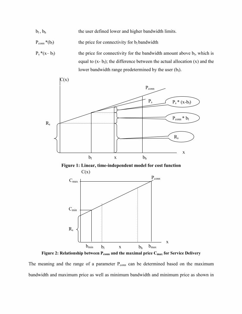
bl , bh the user defined lower and higher bandwidth limits.

Pconn *(bl) the price for connectivity for bl bandwidth

Ps *(x– bl) the price for connectivity for the bandwidth amount above bl, which is

equal to (x- bl); the difference between the actual allocation (x) and the

lower bandwidth range predetermined by the user (bl).

Figure 1: Linear, time-independent model for cost function

Figure 2: Relationship between Pconn and the maximal price Cmax for Service Delivery

The meaning and the range of a parameter Pconn can be determined based on the maximum

bandwidth and maximum price as well as minimum bandwidth and minimum price as shown in

Rs

Ps

Pconn

bl bhxx

C(x)

Ps * (x-bl)

Pconn * bl

Rs

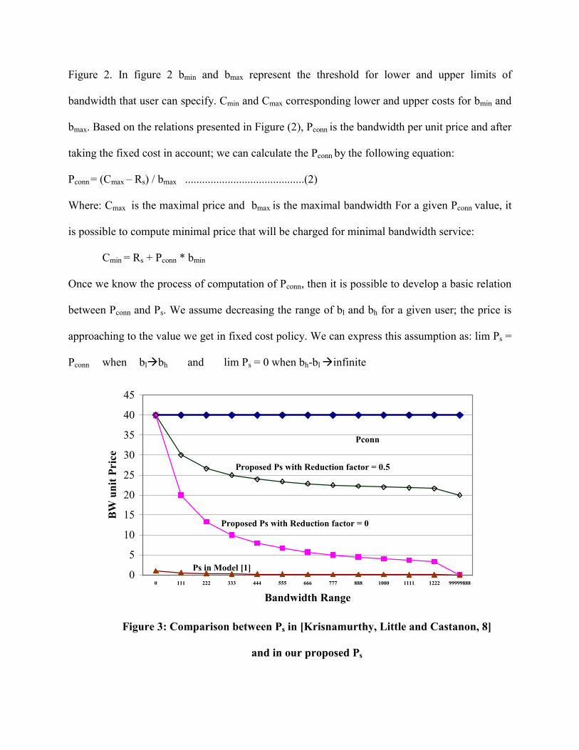
Figure 2. In figure 2 bmin and bmax represent the threshold for lower and upper limits of

bandwidth that user can specify. Cmin and Cmax corresponding lower and upper costs for bmin and

bmax. Based on the relations presented in Figure (2), Pconn is the bandwidth per unit price and after

taking the fixed cost in account; we can calculate the Pconn by the following equation:

Pconn = (Cmax – Rs) / bmax ..........................................(2)

Where: Cmax is the maximal price and bmax is the maximal bandwidth For a given Pconn value, it

is possible to compute minimal price that will be charged for minimal bandwidth service:

Cmin = Rs + Pconn * bmin

Once we know the process of computation of Pconn, then it is possible to develop a basic relation

between Pconn and Ps. We assume decreasing the range of bl and bh for a given user; the price is

approaching to the value we get in fixed cost policy. We can express this assumption as: lim Ps =

Pconn when bl bh and lim Ps = 0 when bh-bl infinite

0

5

10

15

20

25

30

35

40

45

0 111 222 333 444 555 666 777 888 1000 1111 1222 99999888

Bandwidth Range

BW u

nit P

rice

Proposed Ps with Reduction factor = 0

Ps in Model [1]

Pconn

Proposed Ps with Reduction factor = 0.5

Figure 3: Comparison between Ps in [Krisnamurthy, Little and Castanon, 8]

and in our proposed Ps

By using this fact; the smaller the bandwidth interval the higher the Ps parameter becomes, we

can build basic formula for Ps. One possibility of representation is: Ps =Pconn * (bl / bh)

So, if (bl = bh) Then (Ps = Pconn)

The problem with this representation is that user pays minimal price if he selects large bandwidth

range. The user can take undue advantage of this policy when the load on the network is low,

that is the main reason to introduce the concept of reduction factor.

As you can see in Figure 3 above, Ps will be zero if the user requests a very large

bandwidth range. Here, it is important to clearly distinguish between the real application need of

bandwidth (based on its elasticity nature) and user's unrealistic bandwidth range requests.

Usually it is important for service providers to know in advance, what is the real need for

different types of applications and based on that, they can determine the appropriate value for the

minimum and the maximum bandwidth range that the network could be asked to provide. One

way to handle the possibility for those users that ask for a very large bandwidth range just to

keep their prices charges low is to use a reduction factor that minimize the tendency of Ps going

to zero if the bandwidth range is becoming larger and larger. Hence, we propose the reduction

factor as a mean to achieve our goal to encourage users to specify a bandwidth range as their way

of expressing their bandwidth requirements and at the same time, limit them from making

unreasonably wide bandwidth range.

2.2 Reduction Factor (Red)

The parameter Red defines the maximal reduction of price for the same quality of service if the

user extends the scale of service delivery to a maximum. In this case, the range of Ps will depend

on the interval (Red, 1] instead of (0, 1). So, the new definition of the price for scalability range

becomes: Ps =Pconn * (Red + (1–Red) * (bl / bh)) ............................................(3)

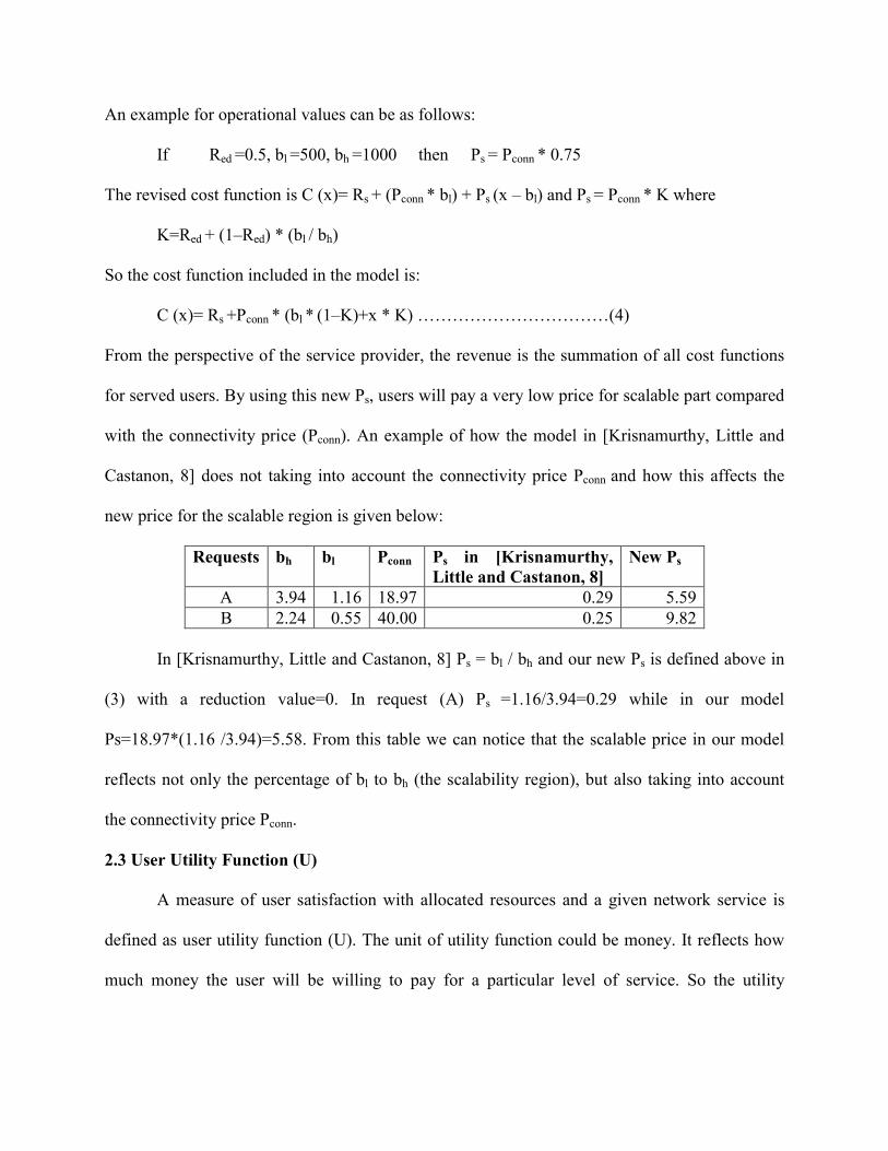
An example for operational values can be as follows:

If Red =0.5, bl =500, bh =1000 then Ps = Pconn * 0.75

The revised cost function is C (x)= Rs + (Pconn * bl) + Ps (x – bl) and Ps = Pconn * K where

K=Red + (1–Red) * (bl / bh)

So the cost function included in the model is:

C (x)= Rs +Pconn * (bl * (1–K)+x * K) ……………………………(4)

From the perspective of the service provider, the revenue is the summation of all cost functions

for served users. By using this new Ps, users will pay a very low price for scalable part compared

with the connectivity price (Pconn). An example of how the model in [Krisnamurthy, Little and

Castanon, 8] does not taking into account the connectivity price Pconn and how this affects the

new price for the scalable region is given below:

Requests bh bl Pconn Ps in [Krisnamurthy, Little and Castanon, 8]

New Ps

A 3.94 1.16 18.97 0.29 5.59 B 2.24 0.55 40.00 0.25 9.82

In [Krisnamurthy, Little and Castanon, 8] Ps = bl / bh and our new Ps is defined above in

(3) with a reduction value=0. In request (A) Ps =1.16/3.94=0.29 while in our model

Ps=18.97*(1.16 /3.94)=5.58. From this table we can notice that the scalable price in our model

reflects not only the percentage of bl to bh (the scalability region), but also taking into account

the connectivity price Pconn.

2.3 User Utility Function (U)

A measure of user satisfaction with allocated resources and a given network service is

defined as user utility function (U). The unit of utility function could be money. It reflects how

much money the user will be willing to pay for a particular level of service. So the utility

function will be 0 when the Allocated resource x is less than bl and in other cases it is nonlinearly

proportional to x (t), the bandwidth allocated at time t.

U (x)=u1 * (bh * x – x2/2) + uc – P (x) ………………………………(5)

Where: u1: Weight factor, which is, corresponds to RS in cost function

uc: Constant – utility for connectivity which is corresponds to Pconn in the cost function

P (x): Penalty function for frequent changes in bandwidth function x

This penalty function does not exist in the model [Krisnamurthy, Little and Castanon, 8].

However, from our point of view, this is a vital factor to be considered because we want to

differentiate between those users that have received large number of decreases and increases in

bandwidth allocation levels compared to other users that have receive fewer number of decreases

and increases. This stability of service level should affect the cost and user utility functions.

To maximize its benefits, the benefit function (B) can be defined as:

B (x) = U (x) – C (x) …………………………………………… (6)

This is the function, which reflects the overall user satisfaction. It is the difference between what

the users get versus what they paid in a certain bandwidth scale.

2.4 Duration interval and time dependent functions

To achieve an efficient model for pricing policy, we have extended user defined parameters so

that each admission request includes a duration interval: [ts, te] where ts is the starting time of the

requested service and te is the finishing time of that service. The knowledge of these intervals is necessary

for the admission control model to determine which request overlaps and when the reserved resources

will be released. Users may know far in advance of their needs and would like to plan their activities by

making advance reservations to ensure that they will not be blocked by the network’s admission control

mechanism. The possibility of time interval specification in advance should be a part of improved pricing

model architecture to provide a better service.

As a special case request for immediate admission will specify starting time ts as now. In a

general case, when starting time is not equal now, we are talking about advanced reservation. A

user that does not know how long a session will last should be able to use a default value or a

value derived from a personal profile. If a resource allocation turns out to be shorter than

needed, it will be possible to renegotiate by calling admission control again with a starting time

now. Only the unused resources can be given to those who are requesting immediate admission,

filling up the remaining bandwidth.

When a new admission request arrives, admission is granted if the new flow would not cause any

delay bounds to be violated or bandwidth limits to be exceeded. These conditions are checked at

all points where new flows begin, at all starting times but also at all ending times. There is a

tradeoff between the amount of state saved by aggregating requests and the flexibility of making

requests. A simple way to aggregate requests is to use time slots. Duration intervals may then

start and finish only at certain points in time. A disadvantage with this scheme is internal

fragmentation: clients may have to reserve longer intervals than they will actually use.

The cost of service delivery is a time dependent function. We introduce the duration

interval [ts, te] for service delivery for a given user, and it defines the limits of integral formula

for a cost function:

C(x,ts,te) =e

s

tt ∫ {Rs +Pconn [bl *(1–K)+x(t)*K]}dt………………………(7)

Or after integrating the constant part:

C (x, ts, te) = [Rs +Pconn * bl * (1–K)]–(te – ts)+Pconn * K * e

s

tt ∫ x (t) dt …………(8)

Where bl ≤ x ( t ) ≤ bh

A new integral formula for the utility function will be:

U (x (t), ts, te)= e

s

tt ∫ [u1 * ( bh * x – x2/2) * uc – P(x)] dt, ……………………(9)

Where P (x) is the penalty function as a nonlinear, quadratic function proportional with a number

of bandwidth changes N2 (x) in a given time interval: P (x)=u2 * N2 (x) where u2 is a weight

factor related to u1 and N2 (x) is a number of discrete increases/decreases in a function x(t) during

a time interval [ts, te]. This function is chosen to reflect the fact that as number of times the

bandwidth allocation level is changed, the value of penalty functions increases more

dramatically. This increase reflects the user satisfaction as number of true bandwidth allocation

levels change.

The time-dependent utility function U and the time-dependent Benefit function B will be:

U (x (t), ts, te)= uc (te – ts)+u1e

s

tt ∫ (bh * x – x2/2) dt – u2 *

e

s

tt ∫ N2

(x) dt…………(10)

B (x (t), ts, te)= K1+[K2 *e

s

tt ∫ x (t) dt]–[K3 *

e

s

tt ∫ x2 (t) dt]–[K4 *

e

s

tt ∫ N2

(t) dt] ……(11)

Where K1 =(uc – Rs – Pconn * bl (1 – K))(te – ts), K2 =u1* bh – Pconn * K and K3 =u1/2 and K4 = u2

Equations (10) and (11) is the same functions we described above on (5) and (6) but in an

integral formulation.

2.5 Discretization of the model for pricing policy

In order to perform discrete event simulation, the discrete model is derived in this section.

The development of a model for a pricing policy in a discrete domain is based on two important

assumptions:

• The changes in a function x(t), and therefore in functions C, U, B, are only in discrete time

intervals. We can define ∆t as a minimal interval for his changes. Every other periods that

longer can be expressed as an integer multiple of ∆t.

• The changes in values of a bandwidth function x (t) are also discrete. The minimal bandwidth

increase / decrease depends on technical specifications in a network, and we will define this

interval as b.

Based on two discrete values ∆t and ∆b, and derived relation te=ts +n * ∆t for the functions C and

U in our model, are given in a form:

C (x(t), ts, n)= Rs * n *∆t + Pconn * bl * (1 – K) * n * ∆t + Pconn * K ∆t i=0∑n-1 x (ts + i *∆t);

U (x (t), ts, n) =

uc n ∆t + u1 ∆t bh . i=0∑n-1 x (ts + i ∆t) +u1 ∆t/2 i=0∑n-1 x2 (ts + i ∆t) – u2 ∆t i=0∑n-1 N2 (ts+ i ∆t)

U2 = u1 (r – ½)∆b2/q;

B(X(t),ts,n)= (uc – Rs – Pconn bl (1– K)) * n∆t +(u1 bh – Pconn K) ∆t * i=0∑n-1 x (ts+i∆t) u1 ∆t/2 i=0∑n-1

x2(ts+i∆t)+u1∆t((bh – bl)/ ∆b – 1/2). ∆b2/q * i=0∑n-1N2(ts+i∆t)

Where q is the number of negative changes in function x (t), and r =(bh – bl)/ ∆b.

2.6 Admission Control Policy

The admission control mechanisms assigns values for the function x(t) which is defined

for every user on interval [ts, te]. The basic algorithm for admission control is trying to maximize

the revenue for the services and therefore to maximize the profit, assuming fixed capacity and

cost to provide this capacity. Admission control algorithm is given over time and it is developed

using basic assumption given in [Krisnamurthy, Little and Castanon, 8]. This admission control

is based on the monetary incentives, which is different from many other approaches that deal

with the bandwidth range from the point of view of negotiations by reducing the cell service rate

as a way to minimize the blocking possibility [Fulp, Reeves, 5]. However, in this approach there

is no monetary incentive for users to be exposed to this kind of quality degradation. The

admission control algorithm defines the values of a function x for all discrete time intervals t,

when service exist, i.e. in a time domain [ts, te] when x is not equal to 0. Suppose that ba is

available bandwidth in a given moment t0 for a given user. Then the value of a function x can be

computed based on a relation:

0 for ba< bl

x(t0) = bl +∆b* r * bl / bh (1-α) for bl ≤ba≤ bh

bl +∆b* r * (1- α) for ba> bh

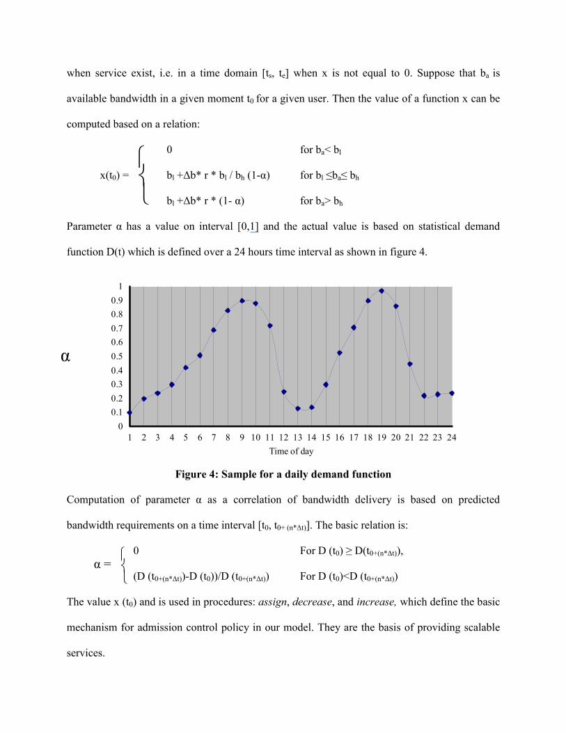
Parameter α has a value on interval [0,1] and the actual value is based on statistical demand

function D(t) which is defined over a 24 hours time interval as shown in figure 4.

00.10.20.30.40.50.60.70.80.9

1

1 2 3 4 5 6 7 8 9 10 11 12 13 14 15 16 17 18 19 20 21 22 23 24Time of day

Figure 4: Sample for a daily demand function

Computation of parameter α as a correlation of bandwidth delivery is based on predicted

bandwidth requirements on a time interval [t0, t0+ (n*∆t)]. The basic relation is:

0 For D (t0) ≥ D(t0+(n*∆t)),

(D (t0+(n*∆t))-D (t0))/D (t0+(n*∆t)) For D (t0)<D (t0+(n*∆t))

The value x (t0) and is used in procedures: assign, decrease, and increase, which define the basic

mechanism for admission control policy in our model. They are the basis of providing scalable

services.

α

α =

Procedure assign uses the value x (t0) to assign the bandwidth interval for every user on a

network controlling the satisfaction of criteria:

1. If ∑ bl ≤ ba then compute x (t0) for all new users and assign them corresponding

bandwidth. At the same time start the procedure increase.

2. If ∑ bl > ba for all new users then assign the bandwidth x (t0) for selected users until for

every new user the relation bl < ba is valid.

3. If ∀ bl > ba then start the procedure decrease.

Procedure decrease decreases assigned resource for the current users to increase the available

resource for new users. Steps are:

1. Sort the users with respect to N values (number of previous increases/decreases)

2. Decrease the resource for the users with the lowest N values minimizing the total Ni for

all current users. Process of decrease is performed in iterations until:

a. ∑ bl for all new users ≤ ba + ∑∆b

b. Value of x comes to bl values for all users.

Procedure increase essentially improves the service by increasing the resources assigned to

current users. It is activated only in a case if after assignment of corresponding resource for

every new user, still exists some available resource ba for current users. Increasing steps are:

1. Sort the current users with respect to bl (decreasing list)

2. Increase the resource xi for a user i on a top of a list for the value:

x= ((bh -xi)(1- α)/( bh - bl)) ∆b Until sum of corrections is less than or equal to the value of ba.

(The complete admission algorithm implemented in the simulation tool is given in Appendix I.)

2.7 Simulation Algorithm

A summary of the simulation algorithm is as follows: We first start with setting up the

appropriate values for the system variables and the customer variable. New requests start their

admission by specifying their low bandwidth (bl), high bandwidth (bh), service starting time (ts)

and service ending time (te). Start the service for ready users and increase their bandwidth to

their bh as long as there exist available bandwidth. Choose one of the following types of service

delivery policy: fixed or scalable with assigning policy based on the historical demand function

or scalable with assigning policy based on the bl for each user. End the service for the finished

users and Increase the available bandwidth with their bandwidth. Then increase the current users

with the available bandwidth to their bh sorted by one of the following options; number of

previous increases and decreases (increasing order), scalability range (bh-bl), combined method

1 and 2 or by the scalability percentage (Ps = bl/bh as in model [Krisnamurthy, Little and

Castanon, 8]). The complete detailed simulation algorithm is given in Appendix I.

2.8 Implementation of Admission Control Algorithm

The simulation starts with initialization then, creates new user as shown in figure 5. In

creating new user there are two possibilities; first, user will be admitted if enough bandwidth is

available. Second, If there is not enough bandwidth to be allocated to the user, At this point, we

can block the new user if we are sure that by decreasing the current users to their low bandwidth

we cannot meet the bandwidth required by the new user.

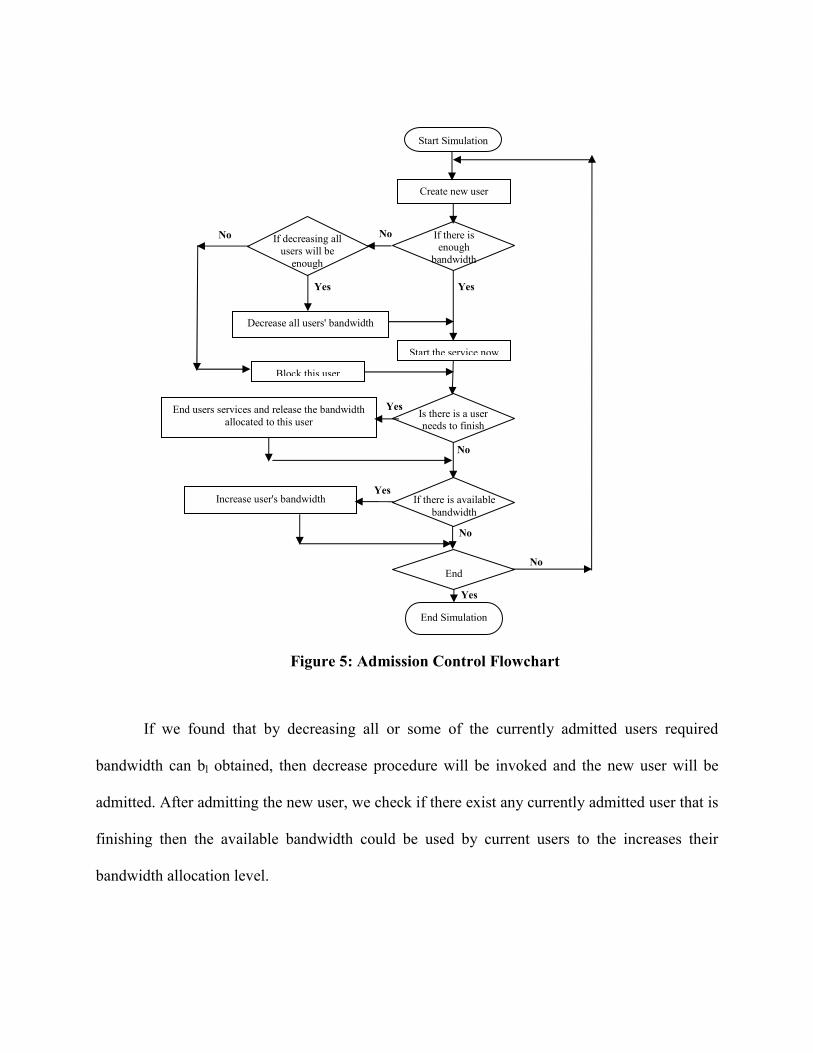
If we found that by decreasing all or some of the currently admitted users required

bandwidth can bl obtained, then decrease procedure will be invoked and the new user will be

admitted. After admitting the new user, we check if there exist any currently admitted user that is

finishing then the available bandwidth could be used by current users to the increases their

bandwidth allocation level.

End Simulation

Create new user

End users services and release the bandwidth allocated to this user

Increase user's bandwidth

Decrease all users' bandwidth

Start the service now

Block this user

If decreasing all users will be

enough

If there is enough

bandwidth

Is there is a user needs to finish

If there is available bandwidth

End

Figure 5: Admission Control Flowchart

Start Simulation

YesYes

No No

Yes

Yes

Yes

No

No

No

This pricing model is attractive for both the users and the network providers. On one

hand, user has the motivation to get better level of service for less cost in case there is available

bandwidth and at the same time a guaranteed minimum level of service at the congestion time.

On the other hand, the network providers by using this pricing model can generate more revenue

for the unutilized network bandwidth and with less number of blocked users.

3 Simulation Tool

The simulation tool has two major components; the customer setup and the server setup.

3.1 Customer setup module:

The customer setup module allows the user to generate a number of customers with

different admission rate levels, different bandwidth ranges and different service time ranges as

shown in figure 6. The customers’ range parameters are:

1- Minimum and maximum bandwidth ranges (bmin, bmax): These two values are very

important to prevent users to consume the whole available bandwidth, also it gives us the

ability to change those ranges and see what will happen to the number of concurrent users that

the network can serve and the number of blocked users. The relation between the rate of

admission and the maximum and minimum bandwidth ranges could be considered one of the

major factors that affect the number of blocked users and network revenue.

2- Minimum and maximum service time, these values represent the minimum and maximum

amount of time that user can request. They are fixed for all users. These two values are

important and affect the number of concurrent users in the network. If this range is very large,

users will be serviced for a long time, which will decrease the admission probability new

users.

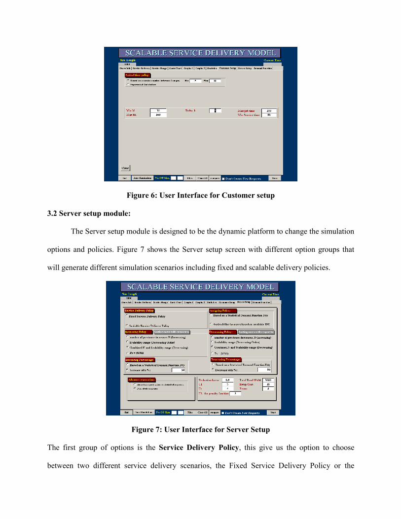
Figure 6: User Interface for Customer setup

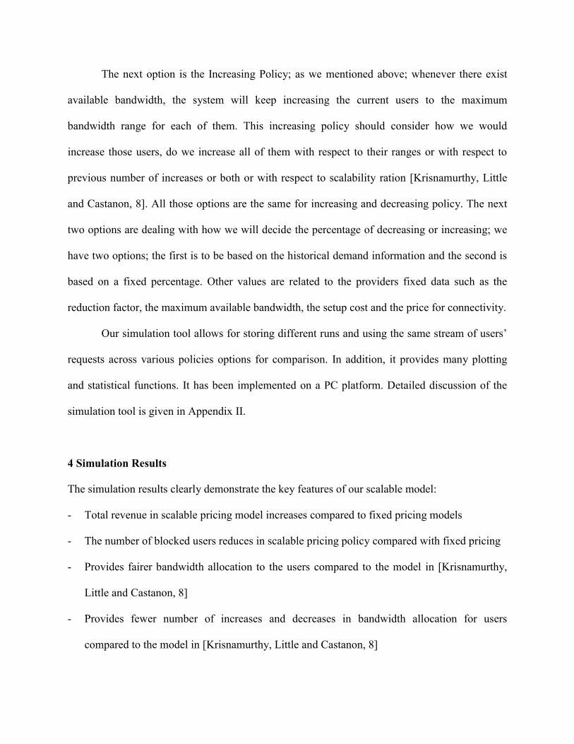
3.2 Server setup module:

The Server setup module is designed to be the dynamic platform to change the simulation

options and policies. Figure 7 shows the Server setup screen with different option groups that

will generate different simulation scenarios including fixed and scalable delivery policies.

Figure 7: User Interface for Server Setup

The first group of options is the Service Delivery Policy, this give us the option to choose

between two different service delivery scenarios, the Fixed Service Delivery Policy or the

Scalable Service Delivery Policy. The Fixed Service Delivery Policy is representing the best

effort QoS policy that means that all admitted users would get the same amount of bandwidth

that was allocated at the time of admission. If there is not enough bandwidth available, all the

new users will be blocked. The other option is the Scalable Service Delivery Policy; this is the

main part of our proposed model. In this option, all the users should provide in advance the range

of bandwidth they need; the minimum acceptable bandwidth (bl) and the maximum bandwidth

they may need (bh), also the starting time and the end time of service. By choosing this option all

user will be admitted to the server and they will get the maximum bandwidth range they asked as

long as there is enough unused bandwidth. If there is no bandwidth available for the new users,

then check is made if decreasing the current logged users to their low bandwidth will provide the

network with the required bandwidth for the new admission or not. If yes then a decrease

scenario will be applied to the current users, else the new user will not be admitted and will be

blocked or revoked.

The next Option Group is the Assigning Policy; this option deals with the amount of

bandwidth that the system will assign to a new user at the starting time. The question here is

should the system gives the users low bandwidth range value and then increases them as in

[Krisnamurthy, Little and Castanon, 8] or assign the higher bandwidth based on historical

demand information if there is available bandwidth. This demand information has a value

between [0,1] for 24 hours as shown in figure 4. In [Odlyzko, 9] they mentioned many examples

for real historical traffic for MCI OC3 Internet trunk on different days of the week over the year

and unsurprisingly it has almost the pattern of usage over the whole year except for specific days

that have some spikes as an exception. We use these demand information values to reduce the

number of increase or decreases in bandwidth allocation level.

The next option is the Increasing Policy; as we mentioned above; whenever there exist

available bandwidth, the system will keep increasing the current users to the maximum

bandwidth range for each of them. This increasing policy should consider how we would

increase those users, do we increase all of them with respect to their ranges or with respect to

previous number of increases or both or with respect to scalability ration [Krisnamurthy, Little

and Castanon, 8]. All those options are the same for increasing and decreasing policy. The next

two options are dealing with how we will decide the percentage of decreasing or increasing; we

have two options; the first is to be based on the historical demand information and the second is

based on a fixed percentage. Other values are related to the providers fixed data such as the

reduction factor, the maximum available bandwidth, the setup cost and the price for connectivity.

Our simulation tool allows for storing different runs and using the same stream of users’

requests across various policies options for comparison. In addition, it provides many plotting

and statistical functions. It has been implemented on a PC platform. Detailed discussion of the

simulation tool is given in Appendix II.

4 Simulation Results

The simulation results clearly demonstrate the key features of our scalable model:

- Total revenue in scalable pricing model increases compared to fixed pricing models

- The number of blocked users reduces in scalable pricing policy compared with fixed pricing

- Provides fairer bandwidth allocation to the users compared to the model in [Krisnamurthy,

Little and Castanon, 8]

- Provides fewer number of increases and decreases in bandwidth allocation for users

compared to the model in [Krisnamurthy, Little and Castanon, 8]

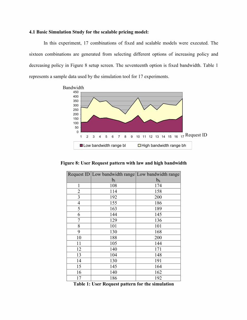
4.1 Basic Simulation Study for the scalable pricing model:

In this experiment, 17 combinations of fixed and scalable models were executed. The

sixteen combinations are generated from selecting different options of increasing policy and

decreasing policy in Figure 8 setup screen. The seventeenth option is fixed bandwidth. Table 1

represents a sample data used by the simulation tool for 17 experiments.

050

100150200250300350400450

1 2 3 4 5 6 7 8 9 10 11 12 13 14 15 16 17

Low bandwidth range bl High bandwidth range bh

Figure 8: User Request pattern with law and high bandwidth

Request ID

Low bandwidth rangebl

Low bandwidth range bh

1 108 174 2 114 158 3 192 200 4 155 186 5 163 189 6 144 145 7 129 136 8 101 101 9 130 168 10 188 200 11 105 144 12 140 171 13 104 148 14 130 191 15 145 164 16 140 162 17 186 192

Table 1: User Request pattern for the simulation

Request ID

Bandwidth

In this experiment, the above 17 users submitted the requests for bandwidth allocation.

Table 2 summarizes the results of 17 experiments. These results are averaged over 10 simulation

runs for each case. In table 2, simulation type refers to the option selected in the set up screen

Figure 7. The simulation type 11 in row one indicates that option number one of increasing

policy and decreasing policy was selected. The simulation type 12 in row two indicates that

option number one of increasing policy and option 2 in the decreasing policy was selected.

Scenario Type

Simulation Type

Served Users

Blocked Users

Up Down Total Revenue

11 16 1 16 5 341805 12 16 1 16 5 341753 13 16 1 16 3 341727 14 16 1 16 5 341763 21 16 1 16 5 341759 22 16 1 16 5 341753 23 16 1 16 3 341727 24 16 1 16 5 341763 31 16 1 16 5 341759 32 16 1 16 5 341762 33 16 1 16 3 341727 34 16 1 16 5 341763 41 16 1 16 5 341750 42 16 1 16 5 341753 43 16 1 16 3 341718

Scalable Scenario

44 16 1 16 5 341754 0 14 3 0 0 309784 Fixed

Scenario 1 14 3 0 0 309784

Table 2: Results for the seventeen cases

The fixed pricing model is indicated as:

0 – Fixed and last used bl and 1 – Fixed with last used bh

It can be observed from the table that in scalable pricing model, 16 users out of 17 were served

and one user was blocked. On the other hand, fixed pricing models blocked three users from

admission. Moreover, the revenue generated from scalable cases is higher than the fixed pricing

model. Within scalable pricing policy cases different options did not make any difference in

number of blocked users but made a minor difference in the total revenue because these options

affect only the order in which bandwidth of current user will be increased or decreased.

4.2 Discussion on Fair bandwidth allocation in scalable pricing policy:

The overall goal of this section is to measure the fairness in terms of number of increases

and decreases for a user based on specified bandwidth range. For example, a user A1 with a

bandwidth range of 50 should have fewer increase or decrease of bandwidth allocation level

compared to another user A2 with a bandwidth range 150. This is due to the fact that user A1 is

paying higher bandwidth cost per allocation unit compared to user A2. Here, we mean by

fairness is to relate number of bandwidth changes (i.e. Increasing or decreasing) to the bandwidth

range requested by the users.

On reference [Krisnamurthy, Little and Castanon, 8] uses scalability range as ratio of

bl/bh. This measure is not fair in determining the sorted order in which users will be identified for

an increase or decrease in bandwidth allocation. A sample snapshot of the simulations data is

given in Table 3. In table 4, the first column shows id’s sorted with the proposed (bh-bl)

approach. The second column shows id’s sorted using approach in [Krisnamurthy, Little and

Castanon, 8]. The results in gray color shows that users are properly ordered for increasing or

decreasing using (bh-bl), rather than bl/bh. In first gray box, according to algorithm in

[Krisnamurthy, Little and Castanon, 8] user ID 14 with range of 145 (from table 3) will be

selected for bandwidth allocation level change compared to user ID 3 with range of 198.

However, in our model user ID 3 will be chosen first for bandwidth allocation level change and

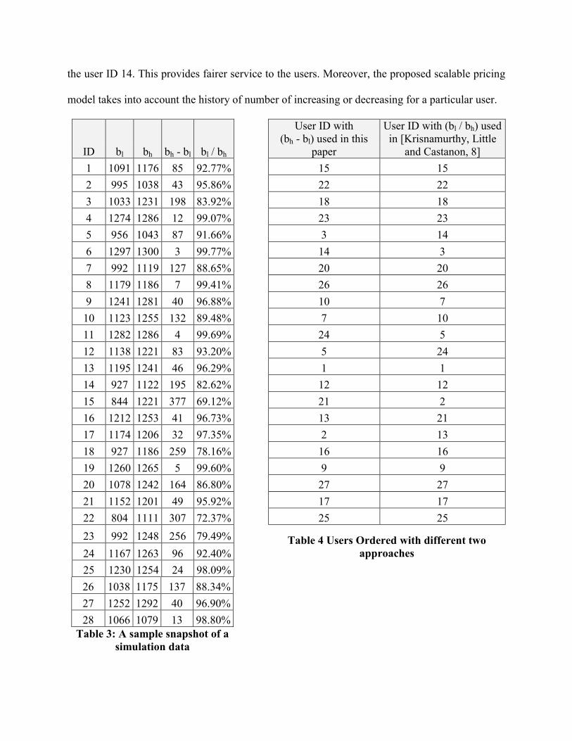
the user ID 14. This provides fairer service to the users. Moreover, the proposed scalable pricing

model takes into account the history of number of increasing or decreasing for a particular user.

ID bl bh bh - bl bl / bh

User ID with (bh - bl) used in this

paper

User ID with (bl / bh) used in [Krisnamurthy, Little

and Castanon, 8] 1 1091 1176 85 92.77% 15 15 2 995 1038 43 95.86% 22 22 3 1033 1231 198 83.92% 18 18 4 1274 1286 12 99.07% 23 23 5 956 1043 87 91.66% 3 14 6 1297 1300 3 99.77% 14 3 7 992 1119 127 88.65% 20 20 8 1179 1186 7 99.41% 26 26 9 1241 1281 40 96.88% 10 7 10 1123 1255 132 89.48% 7 10 11 1282 1286 4 99.69% 24 5 12 1138 1221 83 93.20% 5 24 13 1195 1241 46 96.29% 1 1 14 927 1122 195 82.62% 12 12 15 844 1221 377 69.12% 21 2 16 1212 1253 41 96.73% 13 21 17 1174 1206 32 97.35% 2 13 18 927 1186 259 78.16% 16 16 19 1260 1265 5 99.60% 9 9 20 1078 1242 164 86.80% 27 27 21 1152 1201 49 95.92% 17 17 22 804 1111 307 72.37% 25 25 23 992 1248 256 79.49%

24 1167 1263 96 92.40% Table 4 Users Ordered with different two

approaches 25 1230 1254 24 98.09% 26 1038 1175 137 88.34%

27 1252 1292 40 96.90%

28 1066 1079 13 98.80% Table 3: A sample snapshot of a

simulation data

This is recalculated for each user every time a new user comes to the system. The scalable

pricing model thus guarantees the fairness for every user.

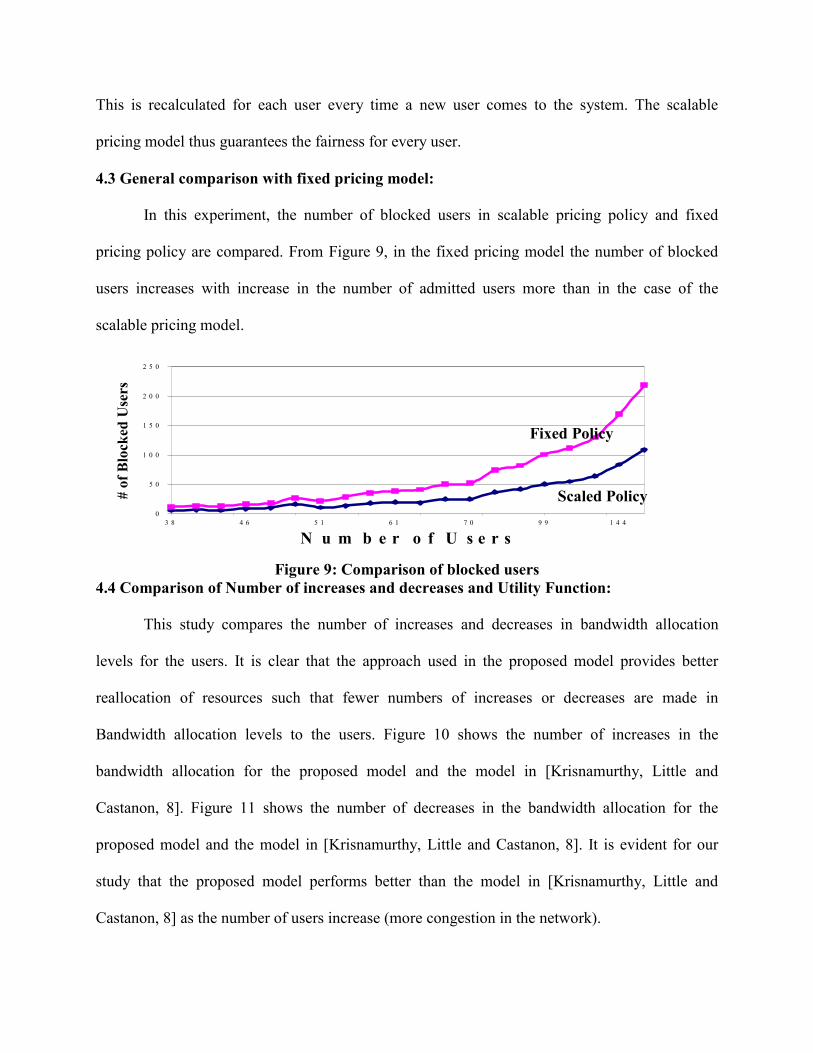
4.3 General comparison with fixed pricing model:

In this experiment, the number of blocked users in scalable pricing policy and fixed

pricing policy are compared. From Figure 9, in the fixed pricing model the number of blocked

users increases with increase in the number of admitted users more than in the case of the

scalable pricing model.

0

5 0

1 0 0

1 5 0

2 0 0

2 5 0

3 8 4 6 5 1 6 1 7 0 9 9 1 4 4

N u m b e r o f U s e r s

# of

Blo

cked

Use

rs

Figure 9: Comparison of blocked users

4.4 Comparison of Number of increases and decreases and Utility Function:

This study compares the number of increases and decreases in bandwidth allocation

levels for the users. It is clear that the approach used in the proposed model provides better

reallocation of resources such that fewer numbers of increases or decreases are made in

Bandwidth allocation levels to the users. Figure 10 shows the number of increases in the

bandwidth allocation for the proposed model and the model in [Krisnamurthy, Little and

Castanon, 8]. Figure 11 shows the number of decreases in the bandwidth allocation for the

proposed model and the model in [Krisnamurthy, Little and Castanon, 8]. It is evident for our

study that the proposed model performs better than the model in [Krisnamurthy, Little and

Castanon, 8] as the number of users increase (more congestion in the network).

Fixed Policy

Scaled Policy

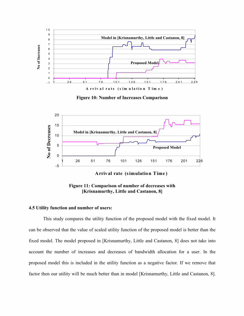
Figure 10: Number of Increases Comparison

Figure 11: Comparison of number of decreases with

[Krisnamurthy, Little and Castanon, 8]

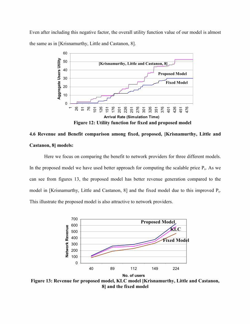
4.5 Utility function and number of users:

This study compares the utility function of the proposed model with the fixed model. It

can be observed that the value of scaled utility function of the proposed model is better than the

fixed model. The model proposed in [Krisnamurthy, Little and Castanon, 8] does not take into

account the number of increases and decreases of bandwidth allocation for a user. In the

proposed model this is included in the utility function as a negative factor. If we remove that

factor then our utility will be much better than in model [Krisnamurthy, Little and Castanon, 8].

-5

0

5

10

15

20

1 26 51 76 101 126 151 176 201 226

Arrival rate (s imulation Time )

No

of D

ecre

ases

Proposed Model

Model in [Krisnamurthy, Little and Castanon, 8]

- 1

0

1

2

3

4

5

6

7

8

9

1 0

1 2 6 5 1 7 6 1 0 1 1 2 6 1 5 1 1 7 6 2 0 1 2 2 6

A r r i v a l r a t e ( s i m u l a t i o n T i m e )

No

of In

crea

ses

Proposed Model

Model in [Krisnamurthy, Little and Castanon, 8]

0

10

20

30

40

50

60

1 26 51 76 101

126

151

176

201

226

251

276

301

326

351

376

401

426

451

476

Arrival Rate (Simulation Time)

Agg

rega

te U

sers

Util

ity

Proposed Model

Fixed Model

[Krisnamurthy, Little and Castanon, 8]

0100200300400500600700

40 89 112 149 224

No. of users

Net

wor

k R

even

ue

Even after including this negative factor, the overall utility function value of our model is almost

the same as in [Krisnamurthy, Little and Castanon, 8].

Figure 12: Utility function for fixed and proposed model

4.6 Revenue and Benefit comparison among fixed, proposed, [Krisnamurthy, Little and

Castanon, 8] models:

Here we focus on comparing the benefit to network providers for three different models.

In the proposed model we have used better approach for computing the scalable price Ps. As we

can see from figures 13, the proposed model has better revenue generation compared to the

model in [Krisnamurthy, Little and Castanon, 8] and the fixed model due to this improved Ps.

This illustrate the proposed model is also attractive to network providers.

Figure 13: Revenue for proposed model, KLC model [Krisnamurthy, Little and Castanon, 8] and the fixed model

Proposed ModelKLC

Fixed Model

0

10

20

30

40

50

60

2 12 22 32 47 57 69 80 99 112 127 144 161 182 205 220

Number of requests

% B

lock

ed R

eque

sts

4.7 Blocking Probability Comparison:

We define blocking probability as the probability that there are not enough resources to

be allocated to the new requests to fulfill their lowest acceptable bandwidth requirements (bl).

New users continue their admission to the network service as long as there exist enough

bandwidth for applications. Once all the bandwidth is consumed by the current users, the

admission control algorithm examines the scalability region if it has enough for the new request's

bl. If this is the case, it starts the decrease process and then admits the new requests. In our

simulation framework, we added the feature of advance reservation as a part of the server setup

module. Using this feature and by utilizing the daily demand data, it could be predicted if the

user will suffer from blocking or not. This allows users to change their preferences such as

starting time and/or his ending time or even change in bandwidth requirements.

Figure 14: Blocking Portability comparison (Proposed, KLC [Krisnamurthy, Little and Castanon, 8] and fixed model)

Figure 14 above shows that the blocking probability for the three models; fixed, proposed model

with utilizing advance reservation and demand function information and the model in

[Krisnamurthy, Little and Castanon, 8] which has higher blocking probability than in our model.

Fixed Model

Proposed Model

KLC

5 Conclusions

This paper provides an improved and flexible pricing model for information delivery.

This model takes into account the user specified QoS parameters and the network provider

specified limits in delivering the service. The proposed pricing model provides flexibility for

users and the network service providers both. It provides better overall performance compared to

fixed pricing model. It also provides fairer and better allocation of bandwidth than the models

proposed earlier. The model is enhanced by including a penalty function to reflect the user

dissatisfaction because of number of increases or decreases in bandwidth allocation levels within

his service period.

References

[1] Clark, David D. (1996). “A Model for Cost Allocation and Pricing in the Internet.” The Journal of Electronic Publishing, Vol. 2, Issue 1 ISSN 1080-2711 http://www.press.umich.edu/jep/works/ClarkModel.html

[2] Cocchi, Ron. (1993). “Pricing in Computer Networks: Motivation, Formulation, and Example”, IEEE/ACM Transactions on Networking, Vol. 1, No. 6, pp. 614-627.

[3] Degermark, Mikael, Torsten Kohler, Stephen Pink and Olov Schelen. (1997). “Advance Reservations for Predictive Service in the Internet”, Multimedia Systems, Vol. 5, pp. 177-186.

[4] Feng, Wu-chi, Farnam Jahanian, and Stuart Sechrest. (1996). “An optimal bandwidth allocation strategy for the delivery of compressed prerecorded video” ACM/Springer- Verlag Multimedia Systems Journal.

[5] Fulp, Errin W. and Douglas S. Reeves. (1997). “On-Line Dynamic Bandwidth Allocation”, In Proceedings of the International Conference on Network Protocols (ICNP '97)

[6] Fulp, Errin W. and Douglas S. Reeves. (2000). “QoS Rewards and Risks: A Multi-Market Approach to Resource Allocation”, In Proceedings of the IFIP TC6 Networking 2000 Conference, Paris France.

[7] Gupta, Alok, Dale O. Stahl, and Andrew B. Whinston, “A Priority Pricing Approach to Manage Multi-Service Class Networks in Real-Time.” (1996). The Journal of Electronic Publishing, Vol. 2, Issue1 ISSN 1080-2711

[8] Krisnamurthy, T.D.C., T. Little and D. Castanon. (1996). “A Pricing mechanism for Scalable video delivery”, Multimedia Systems, Vol. 4, pp. 328-337.

[9] Odlyzko, A. M. (2000). “The Internet and other networks: Utilization rates and their implications”, Information Economics & Policy Vol. 12 pp. 341-365.

[10] Ott, M., Michelitsch G., Reininger D. and Welling G. (1997). “Adaptive QoS and in Multimedia Systems”, In Proceedings of the 5th International Workshop on Quality of Service (IWQOS'97), Columbia University, New York, USA, Pages 393-396.

[11] Schlembach, A. Skoe, P. Yuan, and E. Knightly. (2001). “Design and Implementation of Scalable Admission Control” In Proceedings of the International Workshop on QoS in Multiservice IP Networks, Rome, Italy.

[12] Youssef, A. Sameh, Ibrahim W. Habib, and Tarek N. Saadawi. (1997). “A Neurocomputing Controller for Bandwidth Allocation in ATM Networks” IEEE Journal on selected areas in communications. Vol. 15. No. 2, pp 191-199

[13] Zhang, Hui and Edward W. Knightly. (1997). “RED-VBR: a renegotiation-based approach to support delay-sensitive VBR video”, Multimedia systems Vol. 5, pp. 164-176.

Appendix I

Simulation Algorithm pseudo code :

Using the discrete model in section 3.4, we have developed a simulation schema for prototyping

various studies. The pseudo code for the simulation is given below:

Call Initialization

While the simulation end time is not reached

If Create New User Counter Flag = 1 then

Call Create New User; Assign to the new user -randomly- his low bandwidth (bl), high bandwidth

(bh), service starting time (ts), ending service time (te)

End If

Recalculate the minimum end time value for the currently started users

// Start the Service for Ready users and increase if Available bandwidth > 0

If there is any waiting users then

If we need to recalculate the minimum starting time then

Recalculate the minimum starting time for the waiting users

End If

End If

If there exist users waiting

If the minimum starting time is reached then

Change the status of users whom their Starting time is reached

Update the current number of waiting users

Change the flag of the need to recalculate the minimum starting time

End If

End If

If there exist users, need to start the service

Choose one of the following types of service

1- Service delivery policy: fixed

2- Service delivery policy: Scalable with assigning policy based on the historical

demand function

3- Service delivery policy: Scalable with assigning policy based on the bl for

each user

Call Start the Service

End If

// Ending the service for the finished users

If there is any users that reached the end time then

Change the status for the users whom their End time is reached

Recalculate the minimum ending time if the flag is set

Change the flag of the need to recalculate the minimum ending time

Increase the available bandwidth

Recalculate the number of serviced users

End If

Update the simulation tables

If there exist users getting serviced

If there exist available bandwidth then

// Increase the current users with the available bandwidth

Call Increase Users bandwidth

The priority in which users will be sorted will be based on the selected

increasing policy:

1- Using the no of previous increasing number increasing order

Or 2- Using the range of scalability bh-bl;

This one of the main objectives of the model; to give the users the incentives to

decide a large range or service instead of small range

Or 3- Combined method 1 and 2

Or 4- Using the original model method which is based on the scalability

percentage Ps=Pconn * bl/bh

End If

End If

Update the Utilization table with the bandwidth and the number of current users

Increment the current simulation time

Loop in the simulation Process

Update the Transactions Data and Update the Cost Calculation

Appendix II

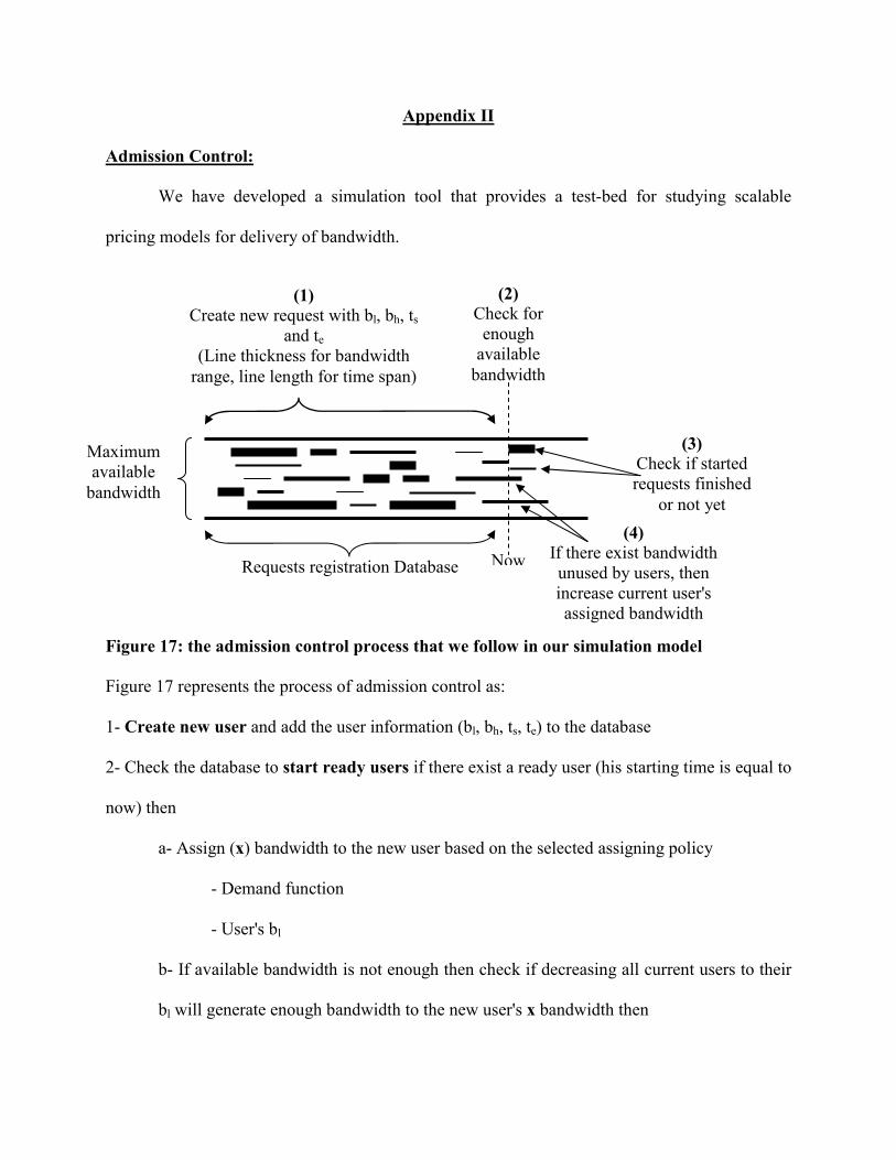
Admission Control:

We have developed a simulation tool that provides a test-bed for studying scalable

pricing models for delivery of bandwidth.

Figure 17: the admission control process that we follow in our simulation model

Figure 17 represents the process of admission control as:

1- Create new user and add the user information (bl, bh, ts, te) to the database

2- Check the database to start ready users if there exist a ready user (his starting time is equal to

now) then

a- Assign (x) bandwidth to the new user based on the selected assigning policy

- Demand function

- User's bl

b- If available bandwidth is not enough then check if decreasing all current users to their

bl will generate enough bandwidth to the new user's x bandwidth then

(3) Check if started requests finished

or not yet

(2) Check for

enough available

bandwidth

Now

(1) Create new request with bl, bh, ts

and te (Line thickness for bandwidth

range, line length for time span)

Maximum available

bandwidth

Requests registration Database

(4) If there exist bandwidth unused by users, then increase current user's assigned bandwidth

- Decrease the number of users based on the selection policy for decreasing,

which determines the users specified for decrease. The following policies are

implemented in simulation:

- Sort users based on number of previous decreases

- Sort users based on Scalability range (bh-bl decreasing order)

- Sort users based on the previous two methods combined

- Sort users based on bl/bh

c- else block or revoke the user (this could be avoided if we check at the admission time

if there will be enough bandwidth for the user or not)

3- Check if there is any user reached his te if yes then:

- End the service for the finished users

4- Increase current user's bandwidth while there exist available bandwidth based on the

selected policy for increasing the bandwidth, this policy determines which users will be

increased first. The following policies are implemented in simulation:

- Sort users based on number of previous increases

- Sort users based on Scalability range (bh-bl decreasing order)

- Sort users based on the previous 2 methods combined

- Sort users based on bl/bh