A rule-based approach for robust clump splitting

Pattern Recognition 39 (2006) 1088–1098www.elsevier.com/locate/patcog

A rule-based approach for robust clump splitting

S. Kumara, S.H. Onga,b,∗, S. Ranganatha, T.C. Ongc, F.T. Chewc

aDepartment of Electrical and Computer Engineering, National University of Singapore, 10 Kent Ridge Crescent, Singapore 119260, SingaporebDivision of Bioengineering, National University of Singapore, 10 Kent Ridge Crescent, Singapore 119260, Singapore

cDepartment of Biological Sciences, National University of Singapore, 10 Kent Ridge Crescent, Singapore 119260, Singapore

Received 14 January 2005; received in revised form 4 November 2005; accepted 4 November 2005

Abstract

This paper presents a robust rule-based approach for the splitting of binary clumps that are formed by objects of diverse shapes andsizes. First, the deepest boundary pixels, i.e., the concavity pixels in a clump, are detected using a fast and accurate scheme. Next,concavity-based rules are applied to generate the candidate split lines that join pairs of concavity pixels. A figure of merit is used todetermine the best split line from the set of candidate lines. Experimental results show that the proposed approach is robust and accurate.� 2005 Pattern Recognition Society. Published by Elsevier Ltd. All rights reserved.

Keywords: Concavity analysis; Overlapping objects; Segmentation; Clump splitting

1. Introduction

The clumping together of objects of interest is a commonphenomenon in a wide variety of image data, e.g., cytolog-ical [1–4] and remotely sensed images [5]. Although a hu-man operator may be able to detect the constituent objects ofinterest based on prior knowledge and perception of textureand structure, it is difficult for a computer-based algorithmto do this automatically. This poses a problem if the aimis to label these objects correctly and perform a populationcount of each class. The splitting of clumps into constituentobjects is thus a vital step that must be performed accuratelyto ensure the overall success of the vision task.

Clump-splitting methods that are available include bi-nary erosion [1,6–8], watershed techniques [9], model-basedapproaches [2,10–12] and concavity analysis [3,4,13–18].A difficulty with erosion-based methods is that they maycompletely erode a constituent object in a clump beforea split occurs. Watershed techniques tend to over-split theclumps. Model-based approaches [2,10–12], besides being

∗ Corresponding author. Department of Electrical and Computer En-gineering, National University of Singapore, 10 Kent Ridge Crescent,Singapore 119260, Singapore. Tel.: +65 6874 2245; fax: +65 6779 1103.

E-mail address: [email protected] (S.H. Ong).

0031-3203/$30.00 � 2005 Pattern Recognition Society. Published by Elsevier Ltd. All rights reserved.doi:10.1016/j.patcog.2005.11.014

computationally expensive, require initialization of themodel parameters [10].

Concavity analysis methods offer an intuitive way ofclump splitting. Such methods have been successfullyimplemented in a variety of application domains such ascervical cancer cells [4], plant cells [13], chromosomes[15], and crushed aggregates [17], to name a few. However,tests have shown that these methods are only applicable forobjects of specific sizes and shapes. Wang [17] reported90% accuracy in splitting clumps comprising overlappingconvex and compactly shaped objects. Fernandez et al. [13]assumed that the gray level variation along the split line wasminimal [13]. This may be true for images in a particularapplication domain but is not generally valid. Liang [15]implemented a scheme for splitting chromosomes that re-portedly worked well but required heuristics incorporatingshape and gray level information. The method is thus notsufficiently general for splitting other types of clumps.

The clump-splitting method proposed in this paper ad-dresses the aforementioned drawbacks. It enables the ac-curate splitting of clumps composed of objects of differentsizes and shapes and with varying degrees of overlap. It isa general method that can be applied to a wide variety ofapplication domains. This is achieved via the implementa-tion of a set of features that guide each decision to split the

S. Kumar et al. / Pattern Recognition 39 (2006) 1088–1098 1089

clump. First, the concavity pixels1 are detected using a fastand accurate scheme. Next, candidate split lines are selectedfrom the set of all possible lines joining any two concav-ity pixels. A candidate split line is one that connects twoconcavity pixels that are close together and lie in concavityregions that are appropriately aligned with respect to eachother. A candidate split line could also connect a concavitypixel with a non-concavity boundary pixel on the clump’scontour if the binary clump has only one concavity region,or if no candidate split line can be found. Finally, we intro-duce a figure of merit that is used to determine the best splitline from the set of candidate lines.

A review of recent concavity analysis methods in Section 2provides the background. Sections 3 and 4 give an overviewof the proposed method and define the features used for de-tecting concavity pixels and candidate split lines. In Section5, the size-invariant feature used for selecting the best splitline from the set of candidate split lines is described. Sec-tion 6 presents training and implementation details. Section7 evaluates the performance of the algorithm on unseen datawhile Section 8 compares its performance against anothermethod and validates each of the features used. Section 9concludes the paper.

2. Review of concavity analysis for clump splitting

In methods based on concavity analysis, a clump is splitby the line joining two concavity pixels on the clump’s con-tour. These methods vary with respect to the technique forlocating the concavity pixels and the cost function used todetect a split path. In general, there are three sequential steps:detection of concavity regions, detection of candidate splitlines and selection of best split line. The best split line is ob-tained recursively until a specific stopping criterion is met.

2.1. Detection of concavity regions or concavity pixels

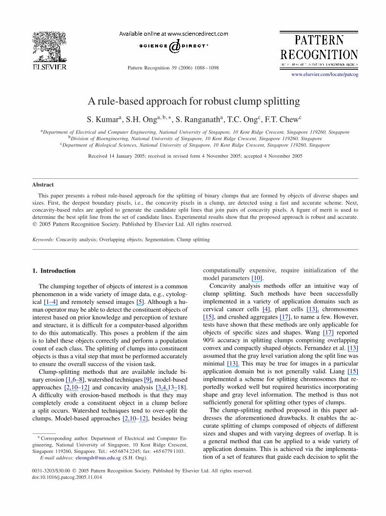
This step detects regions or pixels along the boundarywhere the degree of concavity is high. Such regions or pixelsare regarded as valid concavity regions or pixels. Yeo et al.[4] define a concavity region, Si , as any region bounded bya boundary arc Bi and its corresponding convex hull chordKi (Fig. 1). A concavity region is taken to be valid if itsconcavity degree, Di , and normalized concavity weight, Wi ,exceed their respective threshold values:

Di = |Bi |/|Ki |, Di > DT , (1)

Wi = |Bi |/|Bmax|, Wi > WT , (2)

where | · | denotes length and |Bmax| is the length of thelongest boundary arc in the clump. However, the use of

1 The pixel on the boundary arc (Fig. 1) that has the largest perpen-dicular distance from its corresponding convex hull chord.

K2

K3

B1

B2

B3

K1

Fig. 1. Binary clump with convex hull chords K1, K2 and K3 andcorresponding boundary arcs, B1, B2 and B3.

thresholds DT and WT removes valid concavity regionswhen |Bmax| and Ki are unusually large.

Fernandez et al. [13] and Liang [15] used concavenessmeasures to identify concavity pixels. These measures placemore emphasis on the sharpness of the region surroundingthe concavity pixel rather than on its depth (measured bythe distance of the concavity pixel from the convex hull).Consequently, their definition often leads to the detection ofinvalid concavity regions.

Wang applies a polygonal approximation method followedby corner detection to find the concavity regions [17]. Thepolygonal approximation, however, results in distortion tothe clump’s contour and the natural shape of the constituentobjects.

2.2. Detection of candidate split lines

This step detects candidate split lines from all possiblelines joining any two concavity regions. Yeo et al. consid-ers a line joining two concavity regions to be a valid splitline if its length is less than or equal to those between anytwo pixels that are immediately adjacent to the pixel pair atthe ends of the split line [4]. This approach is computation-ally expensive and results in some incorrect splitting due toboundary irregularities.

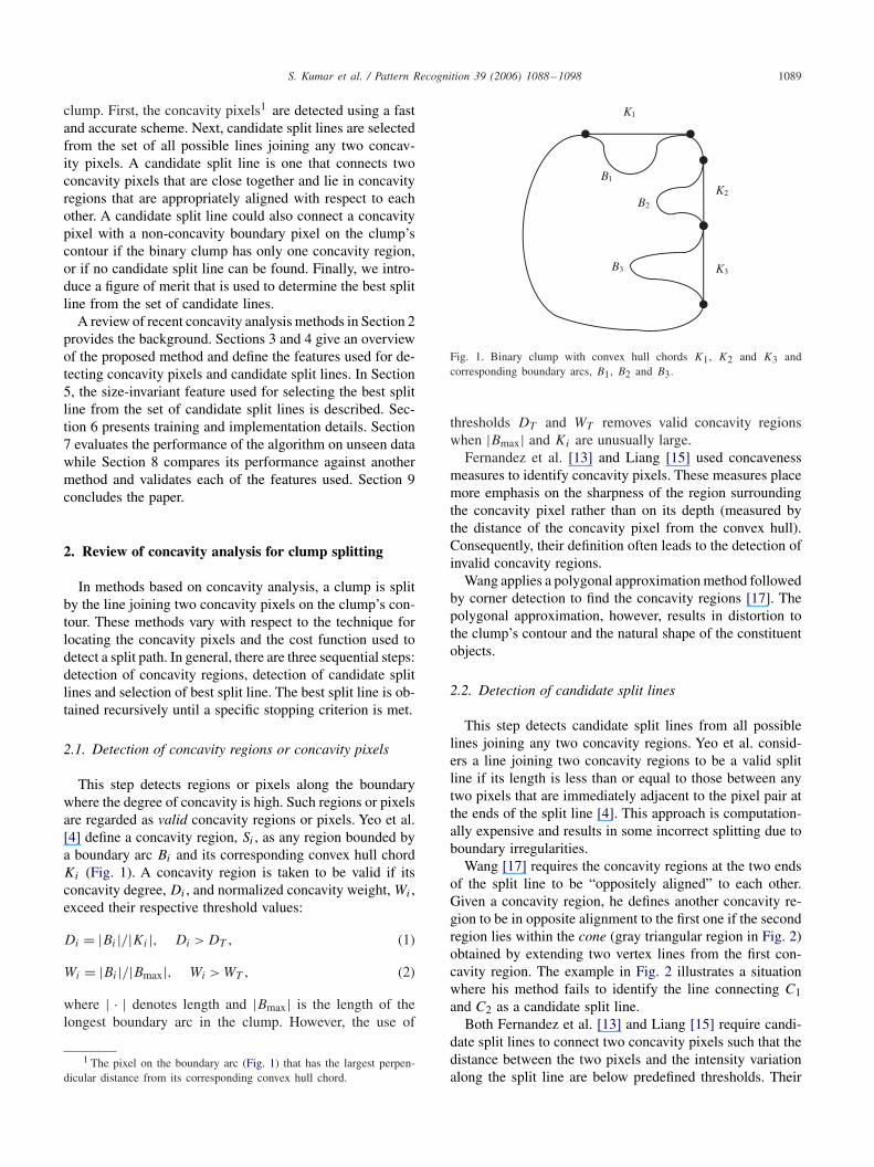
Wang [17] requires the concavity regions at the two endsof the split line to be “oppositely aligned” to each other.Given a concavity region, he defines another concavity re-gion to be in opposite alignment to the first one if the secondregion lies within the cone (gray triangular region in Fig. 2)obtained by extending two vertex lines from the first con-cavity region. The example in Fig. 2 illustrates a situationwhere his method fails to identify the line connecting C1and C2 as a candidate split line.

Both Fernandez et al. [13] and Liang [15] require candi-date split lines to connect two concavity pixels such that thedistance between the two pixels and the intensity variationalong the split line are below predefined thresholds. Their

1090 S. Kumar et al. / Pattern Recognition 39 (2006) 1088–1098

1C

2C Cone of 1C

Fig. 2. Wang’s opposite alignment criterion (from Ref. [17]).

U1

U2

F

Len

gth

of s

plit

line

T1

R

T2

Concaveness

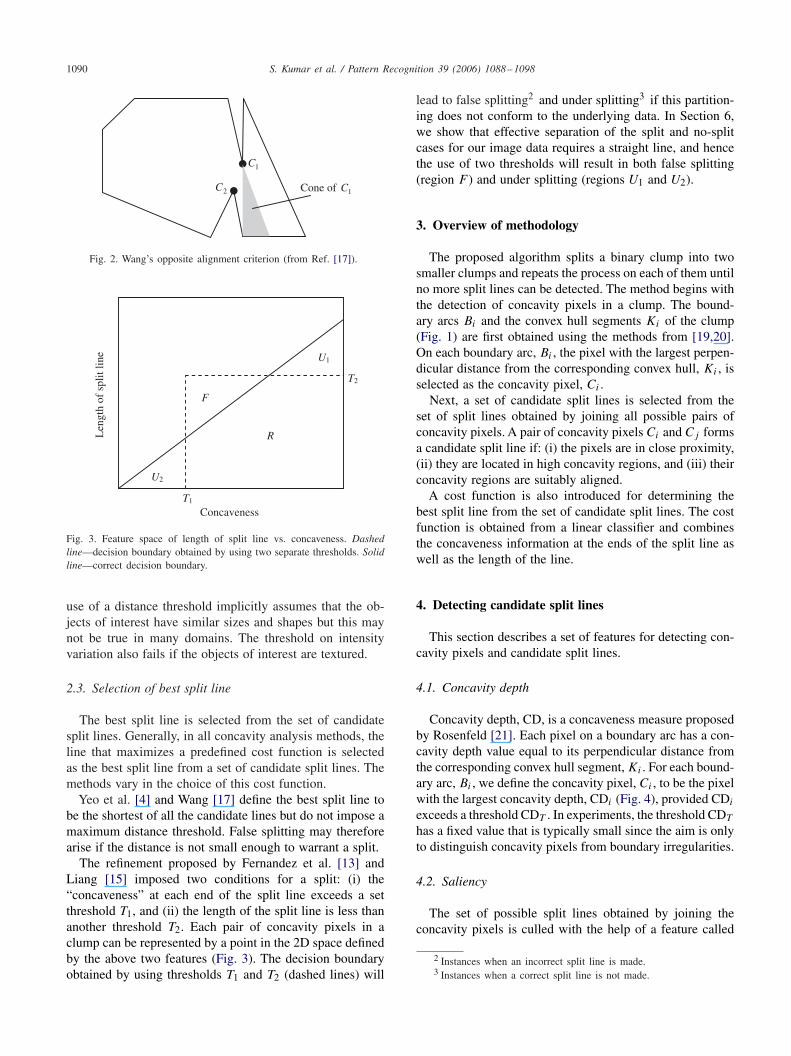
Fig. 3. Feature space of length of split line vs. concaveness. Dashedline—decision boundary obtained by using two separate thresholds. Solidline—correct decision boundary.

use of a distance threshold implicitly assumes that the ob-jects of interest have similar sizes and shapes but this maynot be true in many domains. The threshold on intensityvariation also fails if the objects of interest are textured.

2.3. Selection of best split line

The best split line is selected from the set of candidatesplit lines. Generally, in all concavity analysis methods, theline that maximizes a predefined cost function is selectedas the best split line from a set of candidate split lines. Themethods vary in the choice of this cost function.

Yeo et al. [4] and Wang [17] define the best split line tobe the shortest of all the candidate lines but do not impose amaximum distance threshold. False splitting may thereforearise if the distance is not small enough to warrant a split.

The refinement proposed by Fernandez et al. [13] andLiang [15] imposed two conditions for a split: (i) the“concaveness” at each end of the split line exceeds a setthreshold T1, and (ii) the length of the split line is less thananother threshold T2. Each pair of concavity pixels in aclump can be represented by a point in the 2D space definedby the above two features (Fig. 3). The decision boundaryobtained by using thresholds T1 and T2 (dashed lines) will

lead to false splitting2 and under splitting3 if this partition-ing does not conform to the underlying data. In Section 6,we show that effective separation of the split and no-splitcases for our image data requires a straight line, and hencethe use of two thresholds will result in both false splitting(region F ) and under splitting (regions U1 and U2).

3. Overview of methodology

The proposed algorithm splits a binary clump into twosmaller clumps and repeats the process on each of them untilno more split lines can be detected. The method begins withthe detection of concavity pixels in a clump. The bound-ary arcs Bi and the convex hull segments Ki of the clump(Fig. 1) are first obtained using the methods from [19,20].On each boundary arc, Bi , the pixel with the largest perpen-dicular distance from the corresponding convex hull, Ki , isselected as the concavity pixel, Ci .

Next, a set of candidate split lines is selected from theset of split lines obtained by joining all possible pairs ofconcavity pixels. A pair of concavity pixels Ci and Cj formsa candidate split line if: (i) the pixels are in close proximity,(ii) they are located in high concavity regions, and (iii) theirconcavity regions are suitably aligned.

A cost function is also introduced for determining thebest split line from the set of candidate split lines. The costfunction is obtained from a linear classifier and combinesthe concaveness information at the ends of the split line aswell as the length of the line.

4. Detecting candidate split lines

This section describes a set of features for detecting con-cavity pixels and candidate split lines.

4.1. Concavity depth

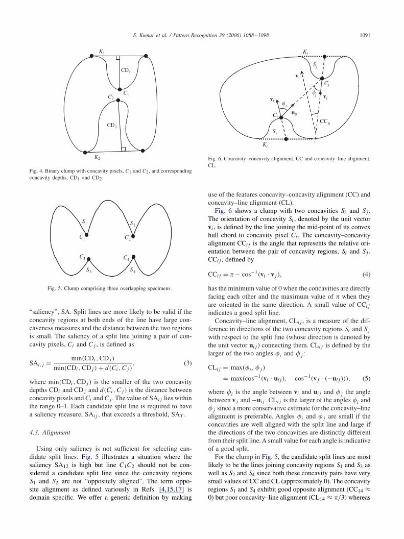
Concavity depth, CD, is a concaveness measure proposedby Rosenfeld [21]. Each pixel on a boundary arc has a con-cavity depth value equal to its perpendicular distance fromthe corresponding convex hull segment, Ki . For each bound-ary arc, Bi , we define the concavity pixel, Ci , to be the pixelwith the largest concavity depth, CDi (Fig. 4), provided CDi

exceeds a threshold CDT . In experiments, the threshold CDT

has a fixed value that is typically small since the aim is onlyto distinguish concavity pixels from boundary irregularities.

4.2. Saliency

The set of possible split lines obtained by joining theconcavity pixels is culled with the help of a feature called

2 Instances when an incorrect split line is made.3 Instances when a correct split line is not made.

S. Kumar et al. / Pattern Recognition 39 (2006) 1088–1098 1091

C1

K1

1CD

C2

K2

2CD

Fig. 4. Binary clump with concavity pixels, C1 and C2, and correspondingconcavity depths, CD1 and CD2.

1S2S

3S 4S

3C

1C 2C

4C

Fig. 5. Clump comprising three overlapping specimens.

“saliency”, SA. Split lines are more likely to be valid if theconcavity regions at both ends of the line have large con-caveness measures and the distance between the two regionsis small. The saliency of a split line joining a pair of con-cavity pixels, Ci and Cj , is defined as

SAi,j = min(CDi , CDj )

min(CDi , CDj ) + d(Ci, Cj ), (3)

where min(CDi , CDj ) is the smaller of the two concavitydepths CDi and CDj and d(Ci, Cj ) is the distance betweenconcavity pixels and Ci and Cj . The value of SAij lies withinthe range 0–1. Each candidate split line is required to havea saliency measure, SAij , that exceeds a threshold, SAT .

4.3. Alignment

Using only saliency is not sufficient for selecting can-didate split lines. Fig. 5 illustrates a situation where thesaliency SA12 is high but line C1C2 should not be con-sidered a candidate split line since the concavity regionsS1 and S2 are not “oppositely aligned”. The term oppo-site alignment as defined variously in Refs. [4,15,17] isdomain specific. We offer a generic definition by making

vjvi

Ci

vi

ijCC

Cj

Kj

Ki

iS

jS

j

i

uij

�

�

Fig. 6. Concavity–concavity alignment, CC and concavity–line alignment,CL.

use of the features concavity–concavity alignment (CC) andconcavity–line alignment (CL).

Fig. 6 shows a clump with two concavities Si and Sj .The orientation of concavity Si , denoted by the unit vectorvi , is defined by the line joining the mid-point of its convexhull chord to concavity pixel Ci . The concavity–concavityalignment CCij is the angle that represents the relative ori-entation between the pair of concavity regions, Si and Sj .CCij , defined by

CCij = � − cos−1(vi · vj ), (4)

has the minimum value of 0 when the concavities are directlyfacing each other and the maximum value of � when theyare oriented in the same direction. A small value of CCij

indicates a good split line.Concavity–line alignment, CLij , is a measure of the dif-

ference in directions of the two concavity regions Si and Sj

with respect to the split line (whose direction is denoted bythe unit vector uij ) connecting them. CLij is defined by thelarger of the two angles �i and �j :

CLij = max(�i , �j )

= max(cos−1(vi · uij ), cos−1(vj · (−uij ))), (5)

where �i is the angle between vi and uij and �j the anglebetween vj and −uij . CLij is the larger of the angles �i and�j since a more conservative estimate for the concavity–linealignment is preferable. Angles �i and �j are small if theconcavities are well aligned with the split line and large ifthe directions of the two concavities are distinctly differentfrom their split line. A small value for each angle is indicativeof a good split.

For the clump in Fig. 5, the candidate split lines are mostlikely to be the lines joining concavity regions S1 and S3 aswell as S2 and S4 since both these concavity pairs have verysmall values of CC and CL (approximately 0). The concavityregions S1 and S4 exhibit good opposite alignment (CC14 ≈0) but poor concavity–line alignment (CL14 ≈ �/3) whereas

1092 S. Kumar et al. / Pattern Recognition 39 (2006) 1088–1098

Ci

P

Ci1 Ci2

CAi

Ki

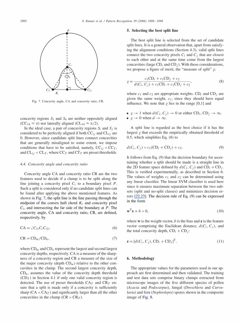
Fig. 7. Concavity angle, CA and concavity ratio, CR.

concavity regions S1 and S4 are neither oppositely aligned(CC14 ≈ �) nor laterally aligned (CL14 ≈ �/2).

In the ideal case, a pair of concavity regions Si and Sj isconsidered to be perfectly aligned if both CCij and CLij are0. However, since candidate split lines connect concavitiesthat are generally misaligned to some extent, we imposeconditions that have to be satisfied, namely, CCij < CCT ,and CLij < CLT , where CCT and CTT are preset thresholds.

4.4. Concavity angle and concavity ratio

Concavity angle CA and concavity ratio CR are the twofeatures used to decide if a clump is to be split along theline joining a concavity pixel Ci to a boundary pixel P .Such a split is considered only if no candidate split lines canbe found after applying the above mentioned features. Asshown in Fig. 7, the split line is the line passing through themidpoint of the convex hull chord Ki and concavity pixelCi , and intersecting the far side of the boundary at P . Theconcavity angle, CA and concavity ratio, CR, are defined,respectively, by

CA = � Ci1CiCi2, (6)

CR = CDm/CDn, (7)

where CDm and CDn represent the largest and second largestconcavity depths, respectively. CA is a measure of the sharp-ness of a concavity region and CR a measure of the size ofthe major concavity (depth CDm) relative to the other con-cavities in the clump. The second largest concavity depth,CDn, assumes the value of the concavity depth threshold(CDT ) in Section 4.1 if only one valid concavity region isdetected. The use of preset thresholds CAT and CRT en-sure that a split is made only if a concavity is sufficientlysharp (CA < CAT ) and significantly larger than all the otherconcavities in the clump (CR > CRT ).

5. Selecting the best split line

The best split line is selected from the set of candidatesplit lines. It is a general observation that, apart from satisfy-ing the alignment conditions (Section 4.3), valid split linesconnect the two concavity pixels Ci and Cj that are closestto each other and at the same time come from the largestconcavities (large CDi and CDj ). With these considerations,we propose a figure of merit, the “measure of split” �:

� = c1CDi + c1CDj + c2

d(Ci, Cj ) + c1CDi + c1CDj + c2, (8)

where c1 and c2 are appropriate weights. CDi and CDj aregiven the same weight, c1, since they should have equalinfluence. We note that � lies in the range [0,1] and

• � → 1 when d(Ci, Cj ) → 0 or either CDi , CDj → ∞.• � → 0 when d → ∞.

A split line is regarded as the best choice if it has thelargest � that exceeds the empirically obtained threshold of0.5, which simplifies Eq. (8) to

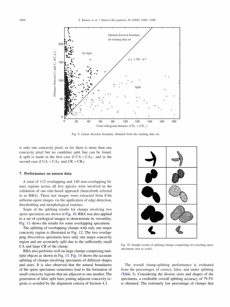
d(Ci, Cj ) < c1(CDi + CDj ) + c2. (9)

It follows from Eq. (9) that the decision boundary for ascer-taining whether a split should be made is a straight line inthe 2D feature space defined by d(Ci, Cj ) and CDi + CDj .This is verified experimentally, as described in Section 6.The values of weights c1 and c2 can be determined usingany linear classifier. The linear SVM classifier is used heresince it ensures maximum separation between the two sub-sets (split and no-split classes) and minimizes decision er-rors [22,23]. The decision rule of Eq. (9) can be expressedin the form

wTz + b > 0, (10)

where w is the weight vector, b is the bias and z is the featurevector comprising the Euclidean distance, d(Ci, Cj ), andthe total concavity depth, CDi + CDj :

z = [d(Ci, Cj ), CDi + CDj ]T. (11)

6. Methodology

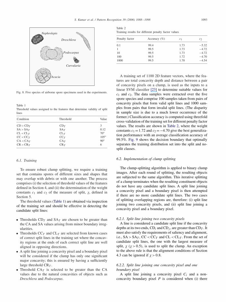
The appropriate values for the parameters used in our ap-proach are first determined and then validated. The trainingand test data sets comprise binary clumps extracted frommicroscope images of the five different species of pollen(Acacia and Podocarpus), fungal (Dreschlera and Curvu-laria) and fern (Nephrolepis) spores shown in the compositeimage of Fig. 8.

S. Kumar et al. / Pattern Recognition 39 (2006) 1088–1098 1093

Curvularia

Acacia

Podocarpus

Dreschlera

Nephrolepis

Fig. 8. Five species of airborne spore specimens used in the experiments.

Table 1Threshold values assigned to the features that determine validity of splitlines

Condition Threshold Value

CD > CDT CDT 3SA > SAT SAT 0.12CL < CLT CLT 70◦CC < CCT CCT 105◦CA < CAT CAT 90◦CR > CRT CRT 6

6.1. Training

To ensure robust clump splitting, we require a trainingset that contains spores of different sizes and shapes thatmay overlap with debris or with one another. The processcomprises (i) the selection of threshold values of the featuresdefined in Section 4, and (ii) the determination of the weightconstants c1 and c2 of the measure of split, �, defined inSection 5.

The threshold values (Table 1) are obtained via inspectionof the training set and should be effective in detecting thecandidate split lines:

• Thresholds CDT and SAT are chosen to be greater thanthe CA and SA values arising from minor boundary irreg-ularities.

• Thresholds CCT and CLT are selected from known casesof correct split lines in the training set where the concav-ity regions at the ends of each correct split line are wellaligned in opposing directions.

• A split line joining a concavity pixel and a boundary pixelwill be considered if the clump has only one significantmajor concavity; this is ensured by having a sufficientlylarge threshold CRT .

• Threshold CAT is selected to be greater than the CAvalues due to the natural concavities of objects such asDreschlera and Podocarpus.

Table 2Training results for different penalty factor values

Penalty factor Accuracy (%) c1 c2

0.1 99.4 1.73 −5.321 99.5 1.73 −4.7210 99.5 1.73 −4.72100 99.5 1.72 −4.701000 99.5 1.70 −4.54

A training set of 1100 2D feature vectors, where the fea-tures are total concavity depth and distance between a pairof concavity pixels on a clump, is used as the inputs to alinear SVM classifier [23] to determine suitable values forc1 and c2. The data samples were extracted over the fivespore species and comprise 100 samples taken from pairs ofconcavity pixels that form valid split lines and 1000 sam-ples from pairs that form invalid split lines. (The disparityin sample size is due to a much lower occurrence of theformer.) Classification accuracy is computed using threefoldcross-validation of the training set for different penalty factorvalues. The results are shown in Table 2, where the weightconstants c1 =1.72 and c2 =−4.70 give the best generaliza-tion performance with an average classification accuracy of99.5%. Fig. 9 shows the decision boundary that optimallyseparates the training distribution set into the split and no-split classes.

6.2. Implementation of clump splitting

The clump-splitting algorithm is applied to binary clumpimages. After each round of splitting, the resulting objectsare subjected to the same algorithm. This iterative splittingof a clump terminates when the resulting constituent objectsdo not have any candidate split lines. A split line joininga concavity pixel and a boundary pixel is then attemptedif there are no more candidate split lines. The two casesof splitting overlapping regions are, therefore: (i) split linejoining two concavity pixels, and (ii) split line joining aconcavity pixel and a boundary pixel.

6.2.1. Split line joining two concavity pixelsA line is considered a candidate split line if the concavity

depths at its two ends, CDi and CDj , are greater than CDT . Itmust also satisfy the requirements of saliency and alignment,i.e., SA > SAT , CC < CCT and CL < CLT . From the set ofcandidate split lines, the one with the largest measure ofsplit, � (� > 0.5), is used to split the clump. An exceptionto the above rule is that the alignment conditions of Section4.3 can be ignored if � > 0.8.

6.2.2. Split line joining one concavity pixel and oneboundary pixel

A split line joining a concavity pixel Ci and a non-concavity boundary pixel P is considered when (i) there

1094 S. Kumar et al. / Pattern Recognition 39 (2006) 1088–1098

0 20 40 60 80 100 120 140 160 180

0

50

100

150

200

Optimal decision boundary

for training data set

Total orthogonal distance ( iCD + jCD )

Dis

tanc

e be

twee

n C

ian

d C

j, d(

Ci,C

j)

d = 1.7W - 4.7

Split

No Split

Fig. 9. Linear decision boundary obtained from the training data set.

is only one concavity pixel, or (ii) there is more than oneconcavity pixel but no candidate split line can be found.A split is made in the first case if CA < CAT , and in thesecond case if CA < CAT and CR > CRT .

7. Performance on unseen data

A total of 112 overlapping and 140 non-overlapping bi-nary regions across all five species were involved in thevalidation of our rule-based approach (henceforth referredto as RBA). These test images were extracted from 8-bitairborne-spore images via the application of edge detection,thresholding and morphological routines.

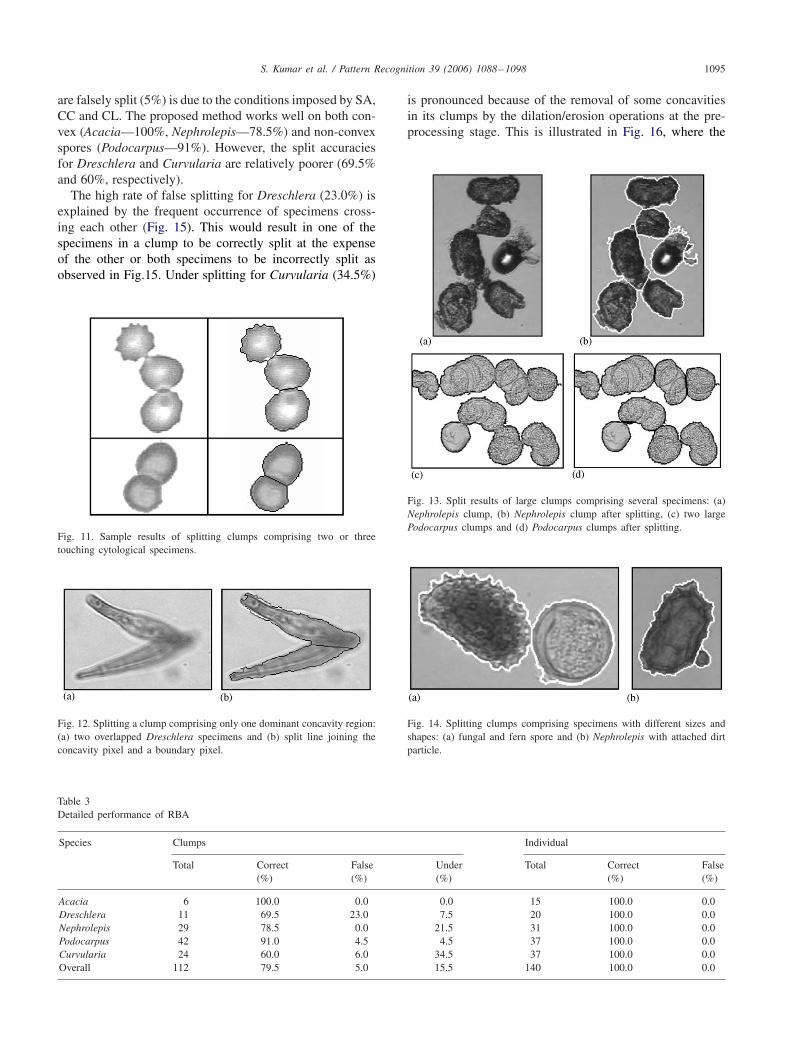
Some of the splitting results for clumps involving twospore specimens are shown in Fig. 10. RBA was also appliedto a set of cytological images to demonstrate its versatility.Fig. 11 shows the results for some overlapping specimens.

The splitting of overlapping clumps with only one majorconcavity region is illustrated in Fig. 12. The two overlap-ping Dreschlera specimens have only one major concavityregion and are accurately split due to the sufficiently smallCA and large CR of the clump.

RBA also performs well on large clumps comprising mul-tiple objects as shown in Fig. 13. Fig. 14 shows the accuratesplitting of clumps involving specimens of different shapesand sizes. It is also observed that the natural boundariesof the spore specimens sometimes lead to the formation ofsmall concavity regions that are adjacent to one another. Thegeneration of false split lines joining adjacent concavity re-gions is avoided by the alignment criteria of Section 4.3.

Fig. 10. Sample results of splitting clumps comprising two touching sporespecimens (not to scale).

The overall clump-splitting performance is evaluatedfrom the percentages of correct, false, and under splitting(Table 3). Considering the diverse sizes and shapes of thespecimens, a creditable overall splitting accuracy of 79.5%is obtained. The extremely low percentage of clumps that

S. Kumar et al. / Pattern Recognition 39 (2006) 1088–1098 1095

are falsely split (5%) is due to the conditions imposed by SA,CC and CL. The proposed method works well on both con-vex (Acacia—100%, Nephrolepis—78.5%) and non-convexspores (Podocarpus—91%). However, the split accuraciesfor Dreschlera and Curvularia are relatively poorer (69.5%and 60%, respectively).

The high rate of false splitting for Dreschlera (23.0%) isexplained by the frequent occurrence of specimens cross-ing each other (Fig. 15). This would result in one of thespecimens in a clump to be correctly split at the expenseof the other or both specimens to be incorrectly split asobserved in Fig.15. Under splitting for Curvularia (34.5%)

Fig. 11. Sample results of splitting clumps comprising two or threetouching cytological specimens.

Fig. 12. Splitting a clump comprising only one dominant concavity region:(a) two overlapped Dreschlera specimens and (b) split line joining theconcavity pixel and a boundary pixel.

Table 3Detailed performance of RBA

Species Clumps Individual

Total Correct False Under Total Correct False(%) (%) (%) (%) (%)

Acacia 6 100.0 0.0 0.0 15 100.0 0.0Dreschlera 11 69.5 23.0 7.5 20 100.0 0.0Nephrolepis 29 78.5 0.0 21.5 31 100.0 0.0Podocarpus 42 91.0 4.5 4.5 37 100.0 0.0Curvularia 24 60.0 6.0 34.5 37 100.0 0.0Overall 112 79.5 5.0 15.5 140 100.0 0.0

is pronounced because of the removal of some concavitiesin its clumps by the dilation/erosion operations at the pre-processing stage. This is illustrated in Fig. 16, where the

Fig. 13. Split results of large clumps comprising several specimens: (a)Nephrolepis clump, (b) Nephrolepis clump after splitting, (c) two largePodocarpus clumps and (d) Podocarpus clumps after splitting.

Fig. 14. Splitting clumps comprising specimens with different sizes andshapes: (a) fungal and fern spore and (b) Nephrolepis with attached dirtparticle.

1096 S. Kumar et al. / Pattern Recognition 39 (2006) 1088–1098

Fig. 15. False splitting of a clump comprising two Dreschlera specimenscrossing each other.

Fig. 16. Reduction in the sizes of the concavity regions in a Curvulariaclump: (a) overlapping and individual Curvularia specimens and (b) binaryclump of Curvularia specimens after dilation/erosion operation.

concavity regions in 16(b) appear smaller than their actualsizes in 16(a).

8. Performance comparison and feature validation

This section compares the performances of RBA and theoptimal dissection method (ODM) of Yeo et al. [14]. It alsovalidates the importance of the features in RBA by study-ing the effects on splitting performance when a feature isremoved or replaced by another feature from ODM. Thefollowing experiments were performed:

• Comparison I—RBA’s concavity depth (CD) vs. ODM’sconcavity degree (D) and normalized concavity weight(W),

• Comparison II—RBA’s measure of split (�) vs. ODM’soptimal dissection requirement, and

• Comparison III—Effect of removing RBA’s saliency (SA)and alignment features (CC and CL).

8.1. Comparison I

In this experiment, we determine the effects on split accu-racy if the concavity pixels, identified using RBA’s CD, are

Table 4Summary of performance comparison and feature validation results

Experiment Clumps Individual

Correct False Under Correct False(%) (%) (%) (%) (%)

RBA 79.5 5.0 15.5 100.0 0Comparison I 58.5 15.0 26.5 99.5 0.5Comparison II 56.0 28.0 16.0 79.0 21.0Comparison III 74.0 12.0 14.0 99.5 0.5

Fig. 17. Shortcomings of ODM’s concavity measure: (a) two overlap-ping Curvularia specimens; concavity region Sa is not detected and (b)Curvularia specimen with overlapping detritus; concavity region Sb isnot detected.

detected only from concavity regions which satisfy ODM’sconcavity degree D and normalized concavity weight W cri-teria with thresholds DT =1.15 and WT =0.25, respectively.As seen in Table 4, the selection of concavity pixels onlyfrom these concavity regions results in lower split accuracyof 58.5% compared to RBA’s 79.5%. The reason for this isthe ineffectiveness of D and W in detecting all valid con-cavity regions, as illustrated in Fig. 17 (where the desiredsplit lines are depicted in white). Fig. 17(a) shows a binaryregion of two overlapping Curvularia specimens; the con-cavity pixel in region Sa is undetected since its correspond-ing boundary arc is significantly smaller than the longestboundary arc, |Bmax|, of the clump. In Fig. 17(b), where theclump consists of a Curvularia specimen and a long detri-tus, the concavity pixel in region Sb is undetected since itsconcavity region lacks sharpness and has a very long convexhull chord, |Ki |.

8.2. Comparison II

In this experiment, we determine the effects on splittingaccuracy if RBA’s method of selecting the best split line isreplaced by ODM’s method. In the latter, the best split lineis the shortest line that satisfies the optimal selection crite-rion and joins two concavity regions that meet the D andW requirements [4]. From Table 4, ODM falsely splits the

S. Kumar et al. / Pattern Recognition 39 (2006) 1088–1098 1097

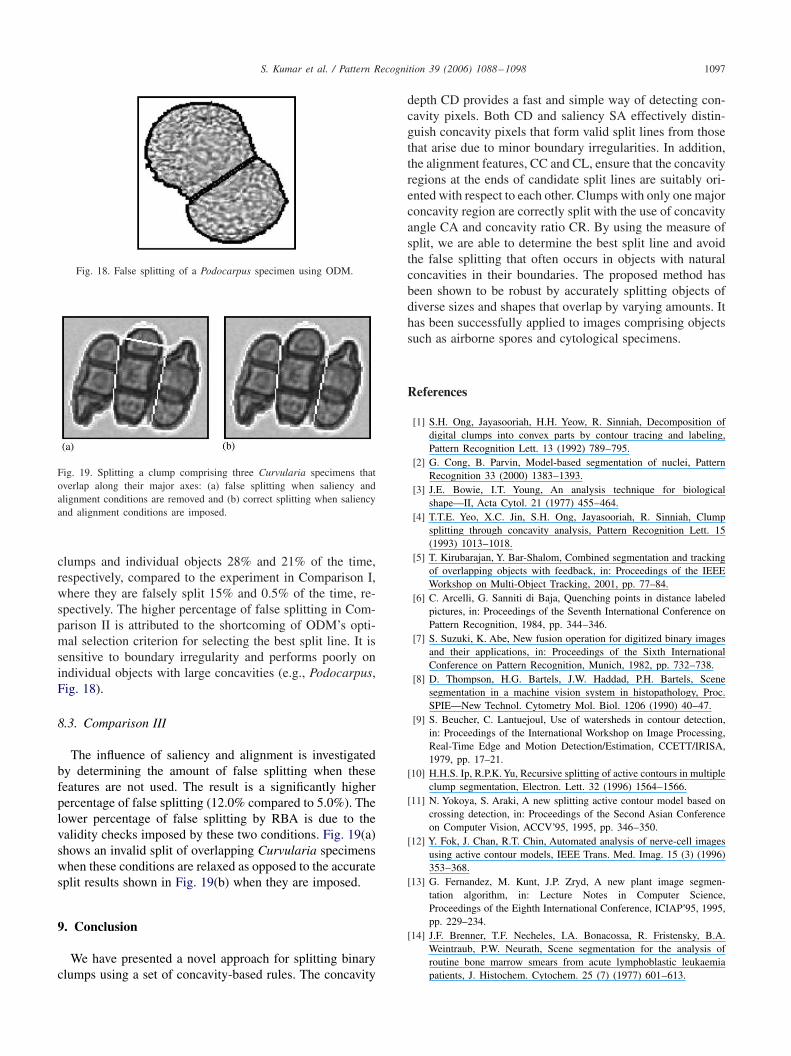
Fig. 18. False splitting of a Podocarpus specimen using ODM.

Fig. 19. Splitting a clump comprising three Curvularia specimens thatoverlap along their major axes: (a) false splitting when saliency andalignment conditions are removed and (b) correct splitting when saliencyand alignment conditions are imposed.

clumps and individual objects 28% and 21% of the time,respectively, compared to the experiment in Comparison I,where they are falsely split 15% and 0.5% of the time, re-spectively. The higher percentage of false splitting in Com-parison II is attributed to the shortcoming of ODM’s opti-mal selection criterion for selecting the best split line. It issensitive to boundary irregularity and performs poorly onindividual objects with large concavities (e.g., Podocarpus,Fig. 18).

8.3. Comparison III

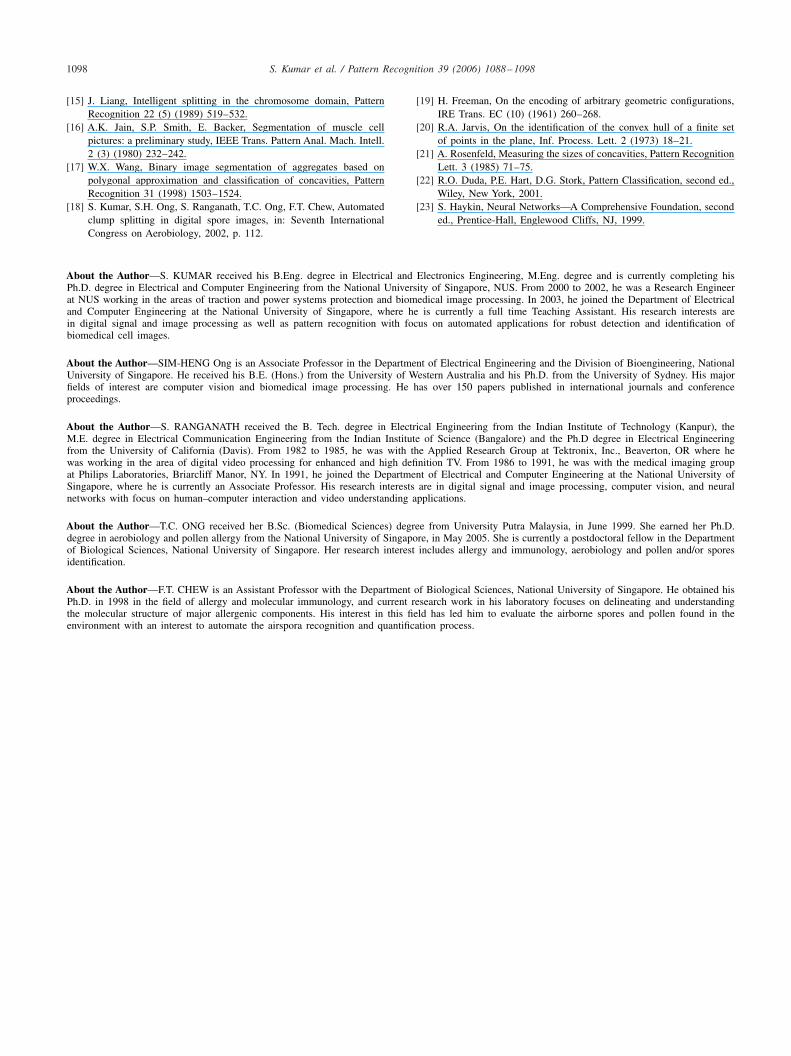
The influence of saliency and alignment is investigatedby determining the amount of false splitting when thesefeatures are not used. The result is a significantly higherpercentage of false splitting (12.0% compared to 5.0%). Thelower percentage of false splitting by RBA is due to thevalidity checks imposed by these two conditions. Fig. 19(a)shows an invalid split of overlapping Curvularia specimenswhen these conditions are relaxed as opposed to the accuratesplit results shown in Fig. 19(b) when they are imposed.

9. Conclusion

We have presented a novel approach for splitting binaryclumps using a set of concavity-based rules. The concavity

depth CD provides a fast and simple way of detecting con-cavity pixels. Both CD and saliency SA effectively distin-guish concavity pixels that form valid split lines from thosethat arise due to minor boundary irregularities. In addition,the alignment features, CC and CL, ensure that the concavityregions at the ends of candidate split lines are suitably ori-ented with respect to each other. Clumps with only one majorconcavity region are correctly split with the use of concavityangle CA and concavity ratio CR. By using the measure ofsplit, we are able to determine the best split line and avoidthe false splitting that often occurs in objects with naturalconcavities in their boundaries. The proposed method hasbeen shown to be robust by accurately splitting objects ofdiverse sizes and shapes that overlap by varying amounts. Ithas been successfully applied to images comprising objectssuch as airborne spores and cytological specimens.

References

[1] S.H. Ong, Jayasooriah, H.H. Yeow, R. Sinniah, Decomposition ofdigital clumps into convex parts by contour tracing and labeling,Pattern Recognition Lett. 13 (1992) 789–795.

[2] G. Cong, B. Parvin, Model-based segmentation of nuclei, PatternRecognition 33 (2000) 1383–1393.

[3] J.E. Bowie, I.T. Young, An analysis technique for biologicalshape—II, Acta Cytol. 21 (1977) 455–464.

[4] T.T.E. Yeo, X.C. Jin, S.H. Ong, Jayasooriah, R. Sinniah, Clumpsplitting through concavity analysis, Pattern Recognition Lett. 15(1993) 1013–1018.

[5] T. Kirubarajan, Y. Bar-Shalom, Combined segmentation and trackingof overlapping objects with feedback, in: Proceedings of the IEEEWorkshop on Multi-Object Tracking, 2001, pp. 77–84.

[6] C. Arcelli, G. Sanniti di Baja, Quenching points in distance labeledpictures, in: Proceedings of the Seventh International Conference onPattern Recognition, 1984, pp. 344–346.

[7] S. Suzuki, K. Abe, New fusion operation for digitized binary imagesand their applications, in: Proceedings of the Sixth InternationalConference on Pattern Recognition, Munich, 1982, pp. 732–738.

[8] D. Thompson, H.G. Bartels, J.W. Haddad, P.H. Bartels, Scenesegmentation in a machine vision system in histopathology, Proc.SPIE—New Technol. Cytometry Mol. Biol. 1206 (1990) 40–47.

[9] S. Beucher, C. Lantuejoul, Use of watersheds in contour detection,in: Proceedings of the International Workshop on Image Processing,Real-Time Edge and Motion Detection/Estimation, CCETT/IRISA,1979, pp. 17–21.

[10] H.H.S. Ip, R.P.K. Yu, Recursive splitting of active contours in multipleclump segmentation, Electron. Lett. 32 (1996) 1564–1566.

[11] N. Yokoya, S. Araki, A new splitting active contour model based oncrossing detection, in: Proceedings of the Second Asian Conferenceon Computer Vision, ACCV’95, 1995, pp. 346–350.

[12] Y. Fok, J. Chan, R.T. Chin, Automated analysis of nerve-cell imagesusing active contour models, IEEE Trans. Med. Imag. 15 (3) (1996)353–368.

[13] G. Fernandez, M. Kunt, J.P. Zryd, A new plant image segmen-tation algorithm, in: Lecture Notes in Computer Science,Proceedings of the Eighth International Conference, ICIAP’95, 1995,pp. 229–234.

[14] J.F. Brenner, T.F. Necheles, I.A. Bonacossa, R. Fristensky, B.A.Weintraub, P.W. Neurath, Scene segmentation for the analysis ofroutine bone marrow smears from acute lymphoblastic leukaemiapatients, J. Histochem. Cytochem. 25 (7) (1977) 601–613.

1098 S. Kumar et al. / Pattern Recognition 39 (2006) 1088–1098

[15] J. Liang, Intelligent splitting in the chromosome domain, PatternRecognition 22 (5) (1989) 519–532.

[16] A.K. Jain, S.P. Smith, E. Backer, Segmentation of muscle cellpictures: a preliminary study, IEEE Trans. Pattern Anal. Mach. Intell.2 (3) (1980) 232–242.

[17] W.X. Wang, Binary image segmentation of aggregates based onpolygonal approximation and classification of concavities, PatternRecognition 31 (1998) 1503–1524.

[18] S. Kumar, S.H. Ong, S. Ranganath, T.C. Ong, F.T. Chew, Automatedclump splitting in digital spore images, in: Seventh InternationalCongress on Aerobiology, 2002, p. 112.

[19] H. Freeman, On the encoding of arbitrary geometric configurations,IRE Trans. EC (10) (1961) 260–268.

[20] R.A. Jarvis, On the identification of the convex hull of a finite setof points in the plane, Inf. Process. Lett. 2 (1973) 18–21.

[21] A. Rosenfeld, Measuring the sizes of concavities, Pattern RecognitionLett. 3 (1985) 71–75.

[22] R.O. Duda, P.E. Hart, D.G. Stork, Pattern Classification, second ed.,Wiley, New York, 2001.

[23] S. Haykin, Neural Networks—A Comprehensive Foundation, seconded., Prentice-Hall, Englewood Cliffs, NJ, 1999.

About the Author—S. KUMAR received his B.Eng. degree in Electrical and Electronics Engineering, M.Eng. degree and is currently completing hisPh.D. degree in Electrical and Computer Engineering from the National University of Singapore, NUS. From 2000 to 2002, he was a Research Engineerat NUS working in the areas of traction and power systems protection and biomedical image processing. In 2003, he joined the Department of Electricaland Computer Engineering at the National University of Singapore, where he is currently a full time Teaching Assistant. His research interests arein digital signal and image processing as well as pattern recognition with focus on automated applications for robust detection and identification ofbiomedical cell images.

About the Author—SIM-HENG Ong is an Associate Professor in the Department of Electrical Engineering and the Division of Bioengineering, NationalUniversity of Singapore. He received his B.E. (Hons.) from the University of Western Australia and his Ph.D. from the University of Sydney. His majorfields of interest are computer vision and biomedical image processing. He has over 150 papers published in international journals and conferenceproceedings.

About the Author—S. RANGANATH received the B. Tech. degree in Electrical Engineering from the Indian Institute of Technology (Kanpur), theM.E. degree in Electrical Communication Engineering from the Indian Institute of Science (Bangalore) and the Ph.D degree in Electrical Engineeringfrom the University of California (Davis). From 1982 to 1985, he was with the Applied Research Group at Tektronix, Inc., Beaverton, OR where hewas working in the area of digital video processing for enhanced and high definition TV. From 1986 to 1991, he was with the medical imaging groupat Philips Laboratories, Briarcliff Manor, NY. In 1991, he joined the Department of Electrical and Computer Engineering at the National University ofSingapore, where he is currently an Associate Professor. His research interests are in digital signal and image processing, computer vision, and neuralnetworks with focus on human–computer interaction and video understanding applications.

About the Author—T.C. ONG received her B.Sc. (Biomedical Sciences) degree from University Putra Malaysia, in June 1999. She earned her Ph.D.degree in aerobiology and pollen allergy from the National University of Singapore, in May 2005. She is currently a postdoctoral fellow in the Departmentof Biological Sciences, National University of Singapore. Her research interest includes allergy and immunology, aerobiology and pollen and/or sporesidentification.

About the Author—F.T. CHEW is an Assistant Professor with the Department of Biological Sciences, National University of Singapore. He obtained hisPh.D. in 1998 in the field of allergy and molecular immunology, and current research work in his laboratory focuses on delineating and understandingthe molecular structure of major allergenic components. His interest in this field has led him to evaluate the airborne spores and pollen found in theenvironment with an interest to automate the airspora recognition and quantification process.